Using R for Customer Analytics

April 2006

Loyalty Matrix, Inc.580 Market StreetSuite 600San Francisco, CA 94104(415) 296-1141http://www.loyaltymatrix.com

Using R for Customer AnalyticsA Practical Introduction to R for Business Analysts

2006

Outline

2

• Introduction:– What is "customer analytics" and why do we do it? – Specific Loyalty Matrix tools & biases. – Implications of working in a business environment.

• Part I - Getting Started: A Brief review of what needs to be done before serious analysis can start.– Sourcing business requirements. – Sourcing raw data. – Profiling raw data. – Data quality control & remediation. – Staging data for analysis.

• Part II - EDA and Basic Statistics: A Step-by-step look at basic customer data with three important variations of the usual business model.

– The fundamentals: counts, amounts and intervals. – The geographical view. – Subscription businesses. – Hospitality businesses. – Big ticket businesses.

• Part III - Mining, Modeling, Segmentation & Prediction: An overview of some useful packages for advanced customer analytics.

– Decision tree methods - rpart, tree, party and randomForest. – Survival methods - survival and friends – Clustering methods - mclust, flexclust. – Association methods - arules.

• Conclusion: – Review of applicable methods by type of client. – The customer analytics check list.

Note: For R setup details see first Appendix slide.

What is “Customer Analytics”?

3

Customer analytics exploit customer behavioral data to identify unique and actionable segments of the customer base. These segments may be used to increase targeting methods. Ultimately, customer analytics enable effective and efficient customer relationship management. The analytical techniques vary based on objective, industry and application, but may be divided into two main categories.

Segmentation techniques segment groups of the customer base that have similar spending and purchasing behavior. Such groups are used to enhance the predictive models as well as improve offer and channel targeting.

Predictive models predict profitability or likelihood and timing of various events based on typical customer behavior and deviationsfrom that behavior.

-- Roman Lenzen, DM Review Magazine, June 2004

Why we do Customer Analytics.

4

If we understand our customers better, we can serve them better.

When we serve our customers better, they will help us be successful.

Background on Loyalty Matrix

5

• Provide customer data analytics to optimize direct marketing resources

• OnDemand platform MatrixOptimizer® (version 3.2)

• Over 20 engagements with Fortune 500 clients

• Experienced team with diverse skills & backgrounds

• 15-person San Francisco firm with an offshore team in Nepal

6

MatrixOptimizer®: Architecture Overview

MatrixOptimizer®: Environment Overview

7

Implications of Business Environment

8

• It’s a Windows / Office world• Focused Inquiries• Large N• Business Interpretation is Essential• Rigor unexpected & unappreciated

– Up to you to supply & enforce

Part I – Getting Started

9

A Brief review of what needs to be done before serious analysis can start.

• Sourcing business requirements. • Sourcing raw data. • Profiling raw data. • Data quality control & remediation. • Staging data for analysis.

Sourcing Business Requirements

10

• Most Important Step!• What are the real business issues?

– Not what analyses to perform– Not immediate concerns of your individual client– The BIG business issue driving project

• How will success of project be measured?– Some Key Performance Indicators (KPI’s)– Measure baseline values before starting

• Ensure KPI’s can be calculated• Get management signoff at onset

• Ensure everyone agrees on key requirements

Sourcing Raw Data

11

• Is data available to answer business questions?– Don’t believe the data structure diagram

• Translating between Marketing & IT– As an outsider, you are allowed stupid questions

• Get lowest level of detail– Not always feasible, but try for it

• BOFF set is typical – “Big ol’ Flat File”

• Avoid Excel as file transfer medium at all costs

• Profile staged raw data to check assumptions about data made when defining problem

Details in Friday’s talk

Profiling Raw Data

12

TriRaw . raw_redemptions . POINTS_USED 5 varchar(6)

#%

Rows90,651100.00

Nulls0

0.00

Distinct2,632

2.90

Empty0

0.00

Numeric90,651100.00

Date29,983

33.08

Min. 80

1st Qu. 3,500

Median 20,000

Mean 18,100

3rd Qu. 25,400

Max.257,000

Distribution of POINTS_USED

Numeric Value

# R

ows

0 50000 100000 150000 200000 250000

030

000

Head: 10000|10000|10000|10000|10000|10000

AMA_Stage . CUSTOMER . GENDER 14 varchar(8000)

#%

Rows471,400

100.00

Nulls209,362

44.41

Distinct3

0.001

Empty0

0.00

Numeric0

0.00

Date0

0.00

M

F

U

Categories in GENDER

# Rows

0 50000 150000 250000

Head: NA|NA|NA|NA|NA|NA

Quality Control & Remediation

13

• Watch out for– The Cancellation Event

• Opt-out Email• Canceling club membership

– Split Identities• Consolidating customer records to the individual & household

– Same Address, similar name, different business key– Tracking Movers

– Magic Values• Especially Dates

• Outliers in amounts & counts probably real– But need checking

• Limit data to problem(s) at hand

• RDBMS Datamart using a Star Schema – See Ralph Kimball: http://www.kimballgroup.com– Holds “Analysis Ready” data

Staging Data for Analysis – Star Schema

14

date

date_id

person

per_identity

location

loc_identity

commerce_contact_fact

ccf_identity

per_identityprod_identitydate_idloc_identitypromo_identityce_identityccf_keyccf_countccf_value

commerce_event

ce_identity

promotion

promo_identity

product

prod_identity

Our “MO” Schema’s Two Main Modules

15

Housekeeping Tables

Links to all tables. Not shown for clarity.

MO Project Wide Definitions Optional AppendsConformed Dimensions

MatrixOptimizer®

dMO – Proposed Schema

Version 3.3.001

16 Apr 06 – Jim Porzak

© 2004-2006 Loyalty Matrix, Inc. All rights reserved.

date

date_id

time_of_day

tod_id

person

per_identity

organization

org_identity

location

loc_identity

address

addr_identity

person_status

pstat_identity

commerce_contact_fact

ccf_identity

ccf_keyccf_countccf_value

commerce_event

ce_identity

contract

con_identity

promotion

promo_identity

product

prod_identity

mo_project

mop_id

mop_project_namemop_versionmop_as_of_date_idmop_etc

mo_codes

code_identity

person_score_fact

psf_identity

organization_score_fact

osf_identity

marketing_contact_fact

mcf_identity

mcf_keyis_usablemember_scoremember_metricmember_valuecontact_valuedays_from_start

marketing_contact_type

mct_identity

cell

cell_identity

campaign

cmpg_identity

media

media_identity

element

elmt_identitty

psychographic

psycho_identity

firmographic

firmo_identity

cmpg_mct, cmpg_elmt, & cmpg_elmt_cell usage definition tables not shown

per_addr, org_addr, & loc_addr usage tables not shown.

Common Resources

Geography Geodemographics Random

load_batch

lb_identity

source

src_identity

Commerce

Marketing

per_org role table not shown.

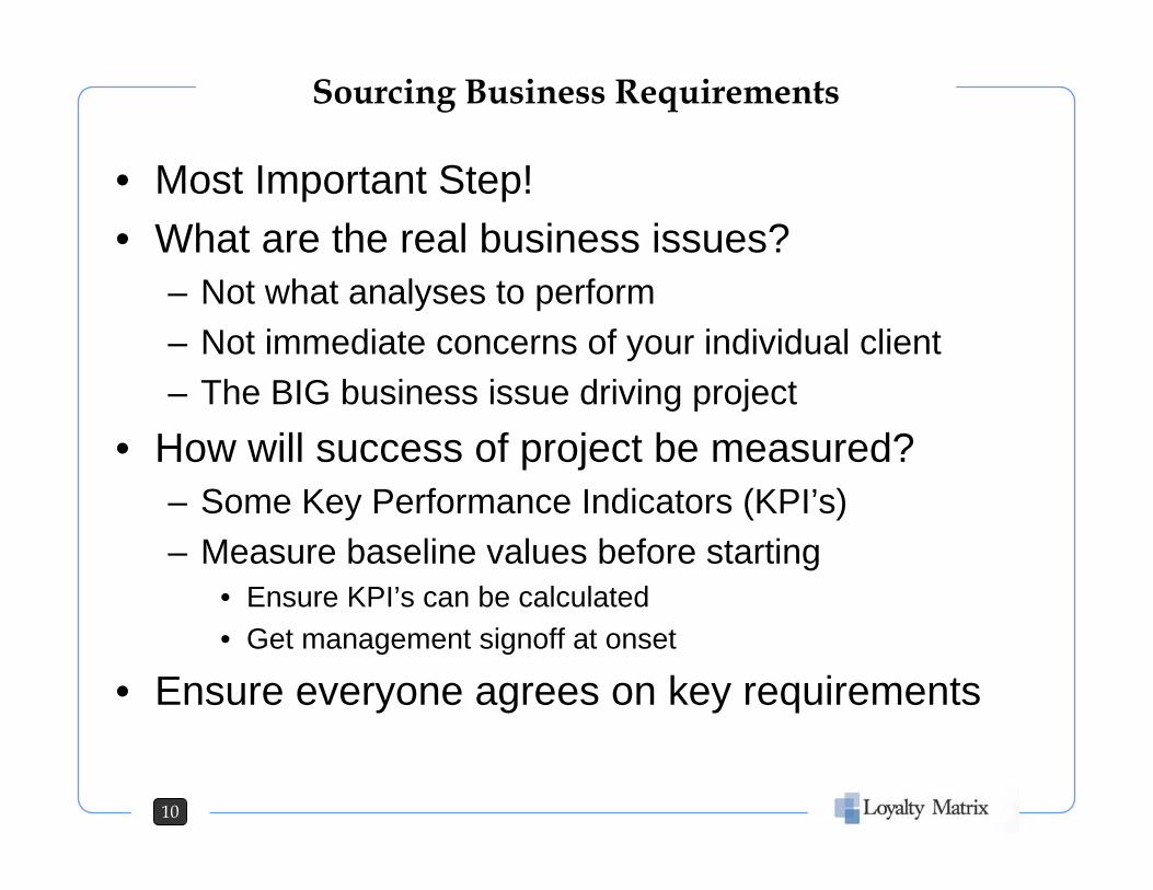
• Use RODBC to load directly from datamart

• Use SQL export & read.table– We’ll use read.delim for tutorial (I like tab delimited)

• Sampling large data sets– RANDOM table trick (two columns: integer identity & runif [0, 9999])

Staging Data for Analysis – Moving to R

16

require(RODBC)cODBC <- odbcConnect("KeyCustomers") # in Windows: odbcConnect("") worksmyQuery <- readChar("../SQL/MyQuery.sql", nchars = 99999) # use cat(myQuery) to viewMyDataFrame <- sqlQuery(cODBC, myQuery)# Fix up datatypes, factors if necessaryMyDataFrame$DatePch <- as.Date(MyDataFrame$DatePch)str(MyDataFrame)head(MyDataFrame)

KeyCustomers <- read.delim("Data/KeyCustomers.txt", row.names = "ActNum")

SELECT SUBT_ID, etc…FROM NewSubscribers nsJOIN Random rON r.identity_key = ns.SUBT_IDAND r.random <= 100 -- for 10% sample

Practical: First Data Set

17

• Manufacturer of parts & tools for construction trades• Direct sales to key accounts• Summary data set with:

– Account ID– Standard Industrial Classification (SIC) code hierarchy– Sales metrics

• Total $ for Year• # Invoices in Year• # Different Products in Year

– Classified by “Potential Size” – created by sales team• Mega, Large, Medium, Small, Mini & Unknown

• Business Questions:– Does Potential Size classification work?– What are SIC differences

Practical: Getting Started (1 of 2)

18

• Check setup of R and our editing environment

R : Copyright 2006, The R Foundation for Statistical ComputingVersion 2.3.0 (2006-04-24)ISBN 3-900051-07-0

R is free software and comes with ABSOLUTELY NO WARRANTY.You are welcome to redistribute it under certain conditions.Type 'license()' or 'licence()' for distribution details.

Natural language support but running in an English locale

R is a collaborative project with many contributors.Type 'contributors()' for more information and'citation()' on how to cite R or R packages in publications.

Type 'demo()' for some demos, 'help()' for on-line help, or'help.start()' for an HTML browser interface to help.Type 'q()' to quit R.

> require(RWinEdt)Loading required package: RWinEdt[1] TRUE>

Practical: Getting Started (2 of 2)

19

• Load our first customer dataset– After looking at it with a text editor!

> # CIwR_01_setup.R> # Get started by loading, checkking & saving Key Customers data> > setwd("c:/Projects/CIwR/R")> dir()[1] "CodeArchive" "Data" "Plots" > dir("Data")[1] "KeyCustomers.txt"> > KeyCustomers <- read.delim("Data/KeyCustomers.txt", row.names = "ActNum")> str(KeyCustomers)`data.frame': 48714 obs. of 10 variables:$ PotSize : Factor w/ 6 levels "LARGE","MEDIUM",..: 5 1 2 2 4 4 4 4 2 2 ...$ Country : Factor w/ 1 level "USA": 1 1 1 1 1 1 1 1 1 1 ...$ IsCore : Factor w/ 1 level "Core": 1 1 1 1 1 1 1 1 1 1 ...$ SIC_Div : Factor w/ 4 levels "Construction",..: 1 1 1 1 1 1 1 1 1 1 ...$ SIC_Group: Factor w/ 11 levels "Building Construction General Contractors And Oper",..: 1 4 4 1 4 4 4 $ SIC_Name : Factor w/ 43 levels "ARCH/ORNAMENTAL METAL",..: 16 11 9 16 40 9 19 18 9 18 ...$ PchPctYr : num 0.274 98.082 67.671 0.000 0.000 ...$ NumInvYr : int 2 60 10 1 1 1 4 1 7 1 ...$ NumProdYr: int 2 81 22 1 3 1 6 1 5 2 ...$ DlrsYr : num 401 31021 6345 643 121 ...> save(KeyCustomers, file = "KeyCustomers.rda")> dir()[1] "CodeArchive" "Data" "KeyCustomers.rda" "Plots"

Part II – EDA & Basic Statistics

20

EDA and Basic Statistics: A Step-by-step look at basic customer data with three important variations of the usual business model.

• The fundamentals: – Counts and amounts and intervals.

• The geographical view. • Subscription businesses. • Hospitality businesses. • Big ticket businesses.

Practical: EDA of Key Customers (1)

21

• Retrieve saved data frame, take a close look

• Observe following & fix– PotSize should be ordered– Country & IsCore contribute no information

> load("KeyCustomers.rda")> str(KeyCustomers)`data.frame': 48714 obs. of 11 variables:$ PotSize : Factor w/ 6 levels "LARGE","MEDIUM",..: 5 1 2 2 4 4 4 4 2 2 ...$ Country : Factor w/ 1 level "USA": 1 1 1 1 1 1 1 1 1 1 ...$ IsCore : Factor w/ 1 level "Core": 1 1 1 1 1 1 1 1 1 1 ...$ SIC_Div : Factor w/ 4 levels "Construction",..: 1 1 1 1 1 1 1 1 1 1 ...$ SIC_Group: Factor w/ 11 levels "Building Construction General Contractors And Oper",..: 1 4 4 1 4 4 ...$ SIC_Name : Factor w/ 43 levels "ARCH/ORNAMENTAL METAL",..: 16 11 9 16 40 9 19 18 9 18 ...$ PchPctYr : num 0.274 98.082 67.671 0.000 0.000 ...$ NumInvYr : int 2 60 10 1 1 1 4 1 7 1 ...$ NumProdYr: int 2 81 22 1 3 1 6 1 5 2 ...$ DlrsYr : num 401 31021 6345 643 121 ...$ ZIP : chr "33063" "37643" "33569" "22151" ...

KeyCustomers$PotSize <- ordered(KeyCustomers$PotSize, levels = c("MEGA", "LARGE", "MEDIUM", "SMALL", "MINI", "UNKNOWN"))# Also, Country & IsCore are superfluous, remove them from analysis setKeyCustomers <- subset(KeyCustomers, select = -c(Country, IsCore))summary(KeyCustomers)save(KeyCustomers, file = "KeyCustomers2.rda") ## Save subseted data frame


22

• Look at variables, starting with Potential Size> attach(KeyCustomers)> table(PotSize)PotSize

MEGA LARGE MEDIUM SMALL MINI UNKNOWN 541 4288 17214 8227 14705 3739

> barplot(table(PotSize), ylab = "# Customers", main = "Distribution Key Customer Potential Size")


23

• Top level of SIC hierarchy shows focus of business> table(SIC_Div)SIC_Div

Construction Manufacturing 46017 1901

Services Transportation, Communications, Electric, Gas, And 725 71

> barplot(table(SIC_Div), ylab = "# Customers", main = "Distribution Key Customer SIC Divisions")


24

• Second level of SIC hierarchy doesn’t plot well

> table(SIC_Group)SIC_GroupBuilding Construction General Contractors And Oper Business Services

17351 152 Communications Construction Special Trade Contractors

71 26625 Electronic And Other Electrical Equipment And Comp Engineering, Accounting, Research, Management, And

30 406 Fabricated Metal Products, Except Machinery And Tr Heavy Construction Other Than Building Constructio

1744 2041 Lumber And Wood Products, Except Furniture Measuring, Analyzing, And Controlling Instruments;

28 99 Miscellaneous Repair Services

167 > barplot(table(SIC_Group), xlab = "# Customers", main = "Distribution Key Customer SIC Groups")


25

• Let’s try horizontal bars– & then put labels in plot area

barplot(sort(table(SIC_Group)), horiz = TRUE, las = 1, xlab = "# Customers", main = "Distribution Key Customer SIC Groups")

bp <- barplot(sort(table(SIC_Group)), horiz = TRUE, las = 1, xlab = "# Customers", main = "Distribution Key Customer SIC Groups",col = "yellow", names.arg = "")

text(0, bp, dimnames(sort(table(SIC_Group)))[[1]], cex = 0.9, pos = 4)


26

• On to continuous variables - $/Year first– Let R do all the work

> hist(DlrsYr, col = “yellow”)

• A couple of interesting things– At least one huge customer– What’s with “minus money”?


27

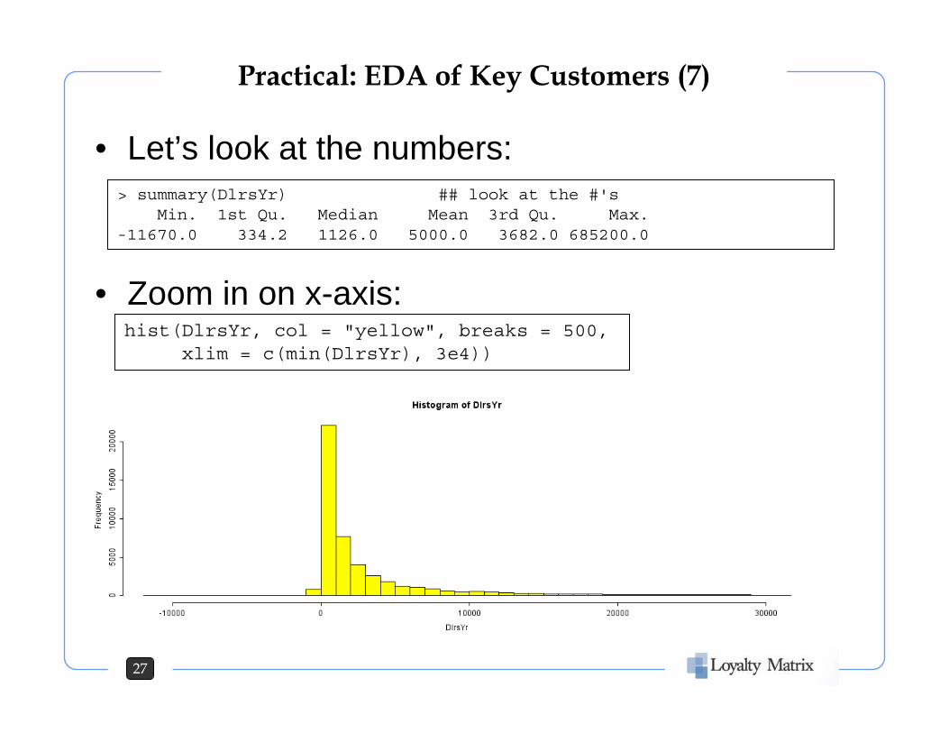
• Let’s look at the numbers:

• Zoom in on x-axis:

> summary(DlrsYr) ## look at the #'sMin. 1st Qu. Median Mean 3rd Qu. Max.

-11670.0 334.2 1126.0 5000.0 3682.0 685200.0

hist(DlrsYr, col = "yellow", breaks = 500, xlim = c(min(DlrsYr), 3e4))


28

• These are supposed to be “key” customers!– Remove those without at least $1/Yr , 1 invoice/Yr, &1 product/Yr

• Plot again. Label y-axis & zoom a bit more on x-axis:

> detach(KeyCustomers)> KeyCustomers <- subset(KeyCustomers, DlrsYr >= 1 & NumInvYr > 0 & NumProdYr > 0)> comment(KeyCustomers) <- "Rev3: subset to just customers with positive Dlrs & Nums."> str(KeyCustomers)`data.frame': 47845 obs. of 9 variables:$ PotSize : Ord.factor w/ 6 levels "MEGA"<"LARGE"<..: 4 2 3 3 5 5 5 5 3 3 ...

<...cut...>- attr(*, "comment")= chr "Rev3: subset to just customers with positive Dlrs & Nums."

> save(KeyCustomers, file = "KeyCustomers3.rda")

hist(DlrsYr, col = "yellow", breaks = 500, xlim = c(min(DlrsYr), 2e4),

ylab = "# Customers")


29

• Right! Log transform all right tailed stuff.• Start with $ per Year:hist(log10(DlrsYr), col = "yellow", ylab = "# Customers",

xlab = "log10 $ per Year")hist(log10(DlrsYr), breaks = 50, col = "yellow", ylab = "# Customers",

xlab = "log10 $ per Year")


30

• Let’s add log10 transforms to data frame & save:log10_DlrsYr <- log10(DlrsYr)log10_NumInvYr <- log10(NumInvYr)log10_NumProdYr <- log10(NumProdYr)detach(KeyCustomers)KCComment <- paste("Rev4: adds log transfroms to data frame;", comment(KeyCustomers))KeyCustomers <- cbind(KeyCustomers, log10_DlrsYr, log10_NumInvYr, log10_NumProdYr)comment(KeyCustomers) <- KCCommentsave(KeyCustomers, file = "KeyCustomers4.rda")rm(log10_DlrsYr, log10_NumInvYr, log10_NumProdYr)attach(KeyCustomers)

> str(KeyCustomers)`data.frame': 47844 obs. of 12 variables:$ PotSize : Ord.factor w/ 6 levels "MEGA"<"LARGE"<..: 4 2 3 3 3 ...

<…cut…>$ log10_DlrsYr : num 2.60 4.49 3.80 2.81 2.08 ...$ log10_NumInvYr : num 0.301 1.778 1.000 0.000 0.000 ...$ log10_NumProdYr: num 0.301 1.908 1.342 0.000 0.477 ...- attr(*, "comment")= chr "Rev4: adds log transfroms to data frame; Rev3:

subset to just customers with positive Dlrs & Nums."

save(KeyCustomers, file = "KeyCustomers4.rda")


31

• Remaining two log10 transformed variables:– hist(log10_NumInvYr, breaks = 50, col = "yellow", ylab = "# Customers",

xlab = "log10 # Invoices per Year")

– hist(log10_NumProdYr, breaks = 50, col = "yellow", ylab = "# Customers", xlab = "log10 # Products per Year")


32

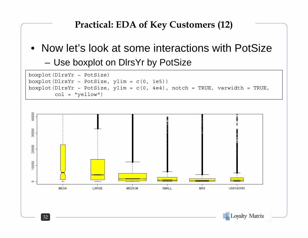
• Now let’s look at some interactions with PotSize– Use boxplot on DlrsYr by PotSize

boxplot(DlrsYr ~ PotSize)boxplot(DlrsYr ~ PotSize, ylim = c(0, 1e5))boxplot(DlrsYr ~ PotSize, ylim = c(0, 4e4), notch = TRUE, varwidth = TRUE,

col = "yellow")


33

• Again calls out for log transformboxplot(log10_DlrsYr ~ PotSize, notch = TRUE, varwidth = TRUE, col = "yellow",

ylab = "log10 $/Yr", main = "Annual Sales by Potential Size")


34

• Boxplot the transforms of the two countsboxplot(log10_NumInvYr ~ PotSize, notch = TRUE, varwidth = TRUE, col = "yellow",

ylab = "log10 $/Yr", main = "# Invoices/Year by Potential Size")

boxplot(log10_NumProdYr ~ PotSize, notch = TRUE, varwidth = TRUE, col = "yellow",ylab = "log10 $/Yr", main = "# Product/Year by Potential Size")


35

• Compute Sales Decile; check against PotSizeiRankCust <- order(DlrsYr, decreasing = TRUE)SalesDecile[iRankCust] <- floor(10.0 * cumsum(DlrsYr[iRankCust]) / sum(DlrsYr)) + 1 aggregate(DlrsYr, list(SalesDecile = SalesDecile), sum) ## a cross checktable(SalesDecile) ## interesting countsrequire(vcd)mosaicplot(PotSize ~ SalesDecile, shade = TRUE,

main = "Potential Size by Actual Sales Decile")


36

• Let’s now look at # products by # invoices– Simple: plot(NumInvYr, NumProdYr)


37

• We now have a better way – bagplot– With much thanks to Peter Wolf & Uni Bielefeld!

require(aplpack)bagplot(NumInvYr, NumProdYr, show.looppoints = FALSE, show.bagpoints = FALSE,

show.whiskers = FALSE, xlab = "# Invoices/Year", ylab = "# Products/Year", main = "Key Customers - # Products by # Invoices")


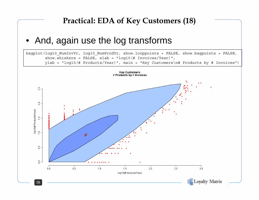
38

• And, again use the log transformsbagplot(log10_NumInvYr, log10_NumProdYr, show.looppoints = FALSE, show.bagpoints = FALSE,

show.whiskers = FALSE, xlab = "log10(# Invoices/Year)", ylab = "log10(# Products/Year)", main = "Key Customers\n# Products by # Invoices")


39

• Also Dollars by Number of Invoicesbagplot(log10_NumInvYr, log10_DlrsYr, show.looppoints = FALSE, show.bagpoints = FALSE,

show.whiskers = FALSE, xlab = "log10(# Invoices/Year)", ylab = "log10($/Year)", main = "Key Customers\n$ by # Invoices")

Summary of Key Customers EDA

40

• Sales department still has a way to go with accounts identified as high “Potential Size “

• Potential fit between log transformed variables• Pareto’s Rule still works:> cumsum(table(SalesDecile))/length(SalesDecile)

1 2 3 4 5 6 7 8 9 10 0.00222 0.00709 0.01532 0.02803 0.04703 0.07568 0.11933 0.19204 0.33149 1.00000

Part III – Mining, Modeling & Segmentation

41

Mining, Modeling, Segmentation & Prediction: An overview of some useful packages for advanced customer analytics.

• Decision tree methods - rpart, tree, party and randomForest.

• Survival methods - survival and friends • Clustering methods - mclust, flexclust. • Association methods - arules.

Random Forests

42

• Random Forest was developed by Leo Breiman of Cal Berkeley, one of the four developers of CART, and Adele Cutler now at Utah State University.

– An extension of single decision tree methods like CART & CHAID.– Many trees are randomly grown to build the forest. All are used in the final result.

• Advantages– Accuracy comparable with modern machine learning methods. (SVMs, neural nets,

Adaboost)– Built in cross-validation using “Out of Bag” data. (Prediction error estimate is a by product)– Large number candidate predictors are automatically selected. (Resistant to over training)– Continuous and/or categorical predicting & response variables. (Easy to set up.)– Can be run in unsupervised for cluster discovery. (Useful for market segmentation, etc.)– Free Prediction and Scoring engines run on PC’s, Unix/Linux & Mac’s. (R version)

• Versions– Original Fortran 77 source code freely available from Breiman & Cutler.

http://www.math.usu.edu/~adele/forests/– R package, randomForest. An adaptation by Andy Liaw of Merck.

http://cran.cnr.berkeley.edu/src/contrib/Descriptions/randomForest.html– Commercialization by Salford Systems.

http://www.salford-systems.com/randomforests.php

• Sample Data from a sports club• Challenge – predict “at-risk” members based on

membership usage data & simple demographics• Training & Test data sets provided:

– MemberTrainingSet.txt (1916 records)– MemberTestSet.txt (1901 records)

• Columns:

Practical: Prediction with RF (1 )

43

• LastCkInDay• DaysSinceLastUse• TotalPaid• MonthlyAmt• MilesToClub• NumExtras1st30d• NumExtrasLast30d• TotalExtras• DaysSinceLastExtra

• MembID (identifier)• Status = M or C • Gender• Age• MembDays• NumUses1st30d• NumUsesLast30d• TotalUses• FirstCkInDay

• Getting Started – Load & understand training set

Practical: Prediction with RF (2)

44

## CIwR_rf.Rrequire(randomForest)setwd("c:/Projects/CIwR/R")dir("Data")

Members <- read.delim("Data/MemberTrainingSet.txt", row.names = "MembID")str(Members)

> str(Members)`data.frame': 1916 obs. of 17 variables:$ Status : Factor w/ 2 levels "C","M": 1 1 1 1 1 1 1 1 1 1 ...$ Gender : Factor w/ 3 levels "F","M","U": 2 2 1 2 2 1 2 1 1 2 ...$ Age : int 21 18 21 21 45 25 21 20 35 15 ...$ MembDays : int 92 98 30 92 31 249 1 92 322 237 ...$ NumUses1st30d : int 11 11 3 6 24 2 0 16 12 6 ...$ NumUsesLast30d : int 6 6 3 1 24 0 0 4 0 0 ...$ TotalUses : int 28 31 3 9 24 6 0 30 38 26 ...$ FirstCkInDay : Factor w/ 556 levels "","2004-01-04",..: 132 264 140 157 507 151 1 124 234 319 ...$ LastCkInDay : Factor w/ 489 levels "","2004-01-15",..: 134 242 83 145 414 111 1 121 280 356 ...$ DaysSinceLastUse : int 3 2 9 11 4 196 NA 12 138 65 ...$ TotalPaid : int 149 136 100 129 75 134 138 149 582 168 ...$ MonthlyAmt : int NA 27 NA NA NA 31 30 NA NA 10 ...$ MilesToClub : int 4 0 0 5 2593 4 5 4 NA 2 ...$ NumExtras1st30d : int 0 0 0 0 0 0 0 0 1 0 ...$ NumExtrasLast30d : int 0 0 0 0 0 0 0 0 0 0 ...$ TotalExtras : int 0 0 0 0 0 0 0 0 6 0 ...$ DaysSinceLastExtra: int NA NA NA NA NA NA NA NA 253 NA ...


45

> summary(Members)Status Gender Age MembDays NumUses1st30d NumUsesLast30d TotalUsesC: 809 F:870 Min. :13.00 Min. : 1.0 Min. : 0.000 Min. : 0.000 Min. : 0.00 M:1107 M:832 1st Qu.:23.00 1st Qu.: 92.0 1st Qu.: 1.000 1st Qu.: 0.000 1st Qu.: 3.00

U:214 Median :29.00 Median :220.0 Median : 4.000 Median : 0.000 Median : 12.00 Mean :32.72 Mean :247.8 Mean : 5.385 Mean : 2.125 Mean : 26.73 3rd Qu.:40.00 3rd Qu.:365.0 3rd Qu.: 8.000 3rd Qu.: 3.000 3rd Qu.: 33.00 Max. :82.00 Max. :668.0 Max. :36.000 Max. :26.000 Max. :340.00 NA's : 1.00

FirstCkInDay LastCkInDay DaysSinceLastUse TotalPaid MonthlyAmt MilesToClub: 236 : 236 Min. : 1.00 Min. : 0.00 Min. : 4.00 Min. : 0.00

2004-06-01: 10 2005-10-28: 56 1st Qu.: 7.00 1st Qu.: 70.75 1st Qu.: 21.00 1st Qu.: 1.00 2004-06-23: 10 2005-10-27: 55 Median : 32.00 Median :135.00 Median : 28.00 Median : 3.00 2004-11-01: 10 2005-10-30: 52 Mean : 75.51 Mean :188.75 Mean : 28.50 Mean : 24.40 2005-02-02: 10 2005-10-26: 47 3rd Qu.:106.00 3rd Qu.:232.25 3rd Qu.: 35.00 3rd Qu.: 7.00 2004-09-13: 9 2005-10-29: 42 Max. :624.00 Max. :961.00 Max. : 94.00 Max. :2609.00 (Other) :1631 (Other) :1428 NA's :236.00 NA's :536.00 NA's : 202.00

NumExtras1st30d NumExtrasLast30d TotalExtras DaysSinceLastExtraMin. : 0.0000 Min. : 0.00000 Min. : 0.000 Min. : 2.00 1st Qu.: 0.0000 1st Qu.: 0.00000 1st Qu.: 0.000 1st Qu.: 55.25 Median : 0.0000 Median : 0.00000 Median : 0.000 Median : 195.00 Mean : 0.4128 Mean : 0.09603 Mean : 1.324 Mean : 229.85 3rd Qu.: 0.0000 3rd Qu.: 0.00000 3rd Qu.: 0.000 3rd Qu.: 376.00 Max. :13.0000 Max. :14.00000 Max. :121.000 Max. : 660.00

NA's :1646.00

• Absolute Dates not useful (at least down to day level)

• RF does not like NA’s!

• Day’s Since Last xxx is NA when no event, use large # days

• Impute remaining NA’s

• Subset out the absolute dates:Members <- subset(Members, select = -c(FirstCkInDay, LastCkInDay))

• Replace days since last NA’s with 999:Members$DaysSinceLastUse[is.na(Members$DaysSinceLastUse)] <- 999

Members$DaysSinceLastExtra[is.na(Members$DaysSinceLastExtra)] <- 999

• Impute remaining NA’s with Random Forests’ impute:Members <- rfImpute(Status ~ ., data = Members)


46

> summary(Members)Status Gender Age MembDays NumUses1st30d NumUsesLast30d TotalUses DaysSinceLastUseC: 809 F:870 Min. :13.00 Min. : 1.0 Min. : 0.000 Min. : 0.000 Min. : 0.00 Min. : 1.0 M:1107 M:832 1st Qu.:23.00 1st Qu.: 92.0 1st Qu.: 1.000 1st Qu.: 0.000 1st Qu.: 3.00 1st Qu.: 9.0

U:214 Median :29.00 Median :220.0 Median : 4.000 Median : 0.000 Median : 12.00 Median : 47.0 Mean :32.71 Mean :247.8 Mean : 5.385 Mean : 2.125 Mean : 26.73 Mean :189.3 3rd Qu.:40.00 3rd Qu.:365.0 3rd Qu.: 8.000 3rd Qu.: 3.000 3rd Qu.: 33.00 3rd Qu.:172.0 Max. :82.00 Max. :668.0 Max. :36.000 Max. :26.000 Max. :340.00 Max. :999.0

TotalPaid MonthlyAmt MilesToClub NumExtras1st30d NumExtrasLast30d TotalExtras DaysSinceLastExtraMin. : 0.00 Min. : 4.00 Min. : 0.000 Min. : 0.0000 Min. : 0.00000 Min. : 0.000 Min. : 2.0 1st Qu.: 70.75 1st Qu.:24.00 1st Qu.: 1.000 1st Qu.: 0.0000 1st Qu.: 0.00000 1st Qu.: 0.000 1st Qu.:999.0 Median :135.00 Median :29.00 Median : 4.000 Median : 0.0000 Median : 0.00000 Median : 0.000 Median :999.0 Mean :188.75 Mean :28.91 Mean : 26.476 Mean : 0.4128 Mean : 0.09603 Mean : 1.324 Mean :890.6 3rd Qu.:232.25 3rd Qu.:33.63 3rd Qu.: 8.426 3rd Qu.: 0.0000 3rd Qu.: 0.00000 3rd Qu.: 0.000 3rd Qu.:999.0 Max. :961.00 Max. :94.00 Max. :2609.000 Max. :13.0000 Max. :14.00000 Max. :121.000 Max. :999.0 >

• Now we can build a forest!– ntree = 500 & mtry = 3 are defaults. Try tuning them.

• Rather good results. Only ~20% overall error rate.– 33% false positive– 13% false negative


47

> Members.rf <- randomForest(Members[-1], Members$Status, data = Members,mtry = 3, ntree = 500, importance = TRUE, proximity = TRUE)

> Members.rfCall:randomForest(x = Members[-1], y = Members$Status, ntree = 500,

mtry = 3, importance = TRUE, proximity = TRUE, data = Members)

Type of random forest: classificationNumber of trees: 500

No. of variables tried at each split: 3

OOB estimate of error rate: 21.4%Confusion matrix:

C M class.errorC 546 263 0.3250927M 147 960 0.1327913

• RF Diagnostics - OOB errors by # trees– Plot(Members.rf)


48

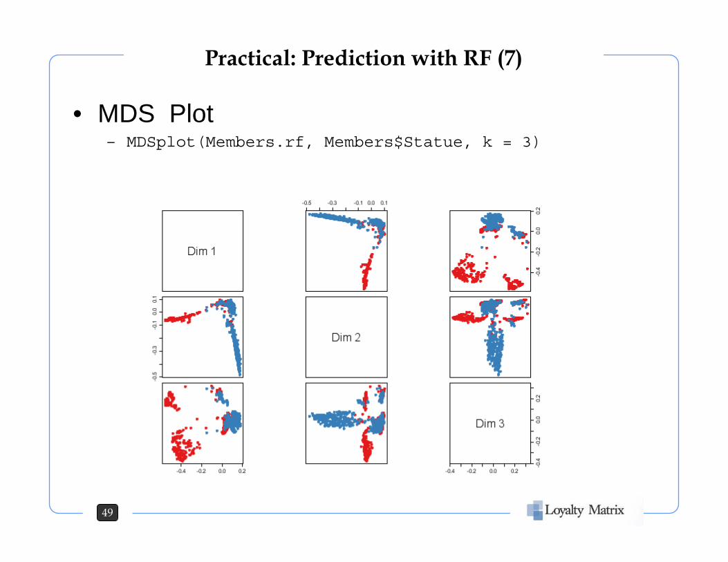
• MDS Plot– MDSplot(Members.rf, Members$Statue, k = 3)


49

• RF Diagnostics – Variable Importance Plot– varImpPlot(Members.rf)


50

• RF Diagnostics – Partial Dependence 1– partialPlot(Members.rf, Members[-1], MembDays)

– abline(h=0, col = "blue")


51

• RF Diagnostics – Partial Dependence 2– partialPlot(Members.rf, Members[-1], DaysSinceLastUse)

– abline(h=0, col = "blue")


52

• RF Diagnostics – Partial Dependence 3– partialPlot(Members.rf, Members[-1], Age)


53

• RF Diagnostics – Prediction on Test Set– Need to do same variable selection & conditioning:


54

## Predictions on test set should be ~ OOB errrorsMembersTest <- read.delim("Data/MemberTestSet.txt", row.names = "MembID")str(MembersTest)summary(MembersTest)MembersTest <- subset(MembersTest, select = -c(FirstCkInDay, LastCkInDay))MembersTest$DaysSinceLastUse[is.na(MembersTest$DaysSinceLastUse)] <- 999MembersTest$DaysSinceLastExtra[is.na(MembersTest$DaysSinceLastExtra)] <- 999MembersTest <- rfImpute(Status ~ ., data = MembersTest)save(MembersTest, file = "MemberTestSetImputed.rda")MembersTest.pred <- predict(Members.rf, MembersTest[-1])

> ct <- table(MembersTest[[1]], MembersTest.pred)> cbind(ct, class.error = c(ct[1,2]/sum(ct[1,]), ct[2,1]/sum(ct[2,])))

C M class.errorC 511 295 0.3660050M 144 951 0.1315068

> (ct[1, 2] + ct[2, 1]) / length(MembersTest$Status) ## Test Set Error[1] 0.2309311

• Need a score? Count the trees.


55

AtRiskScore <- floor(9.99999 * Members.rf$votes[, 1]) + 1barplot(table(AtRiskScore), col = "yellow",

ylab = "# Members", main = "Distribution of At-Risk Scores")

Random Forest Summary

56

• Has yielded practical results in number of cases• Minimal tuning, no pruning required• Black box, with interpretation• Scoring fast & portable

Look at Examples

57

• Questions before we move on?

Questions? Comments?

58

• Email [email protected]• Call 415-296-1141• Visit http://www.LoyaltyMatrix.com• Come by at:

580 Market Street, Suite 600San Francisco, CA 94104

APPENDIX

59

R Setup for Tutorial

60

This is the setup I will be using during the tutorial, you may, of course, change OS, editor, paths to match your own preferences.

• Windows XP SP1 on 2.5GHz P4 w/ 1G RAM.• R Version 2.3.0 • RWinEdt & WinEdt V5.4 or JGR• Following packages will be used

– RWinEdt, aplpack, vcd, survival• Directory Structure

– R’s working directory & source code: C:\Projects\CIwR\R– Tutorial data loaded in: C:\Projects\CIwR\R\Data– Plots will be stored in: C:\Projects\CIwR\R\Plots

• Other tools I like to use– TextPad: www.TextPad.com– DbVisualizer: http://www.dbvis.com/products/dbvis/

R Resources

61

• R & CRAN• R Wiki• Reference Cards

Out Takes

62

• Following outtakes & works in progress

Documents

Using R for Customer Analytics