Embed Size (px)
Citation preview
Using Metric Space Methods to
Analyze Reservoir Uncertainty
Darryl Fenwick Rod Batycky
Streamsim Technologies, Inc.
Outline
• General Modeling workflow
• Classic Sensitivity Analysis
• Metric Spaces for Screening & Sensitivity Analysis
• Applications to Reservoir Modeling
• Conclusions
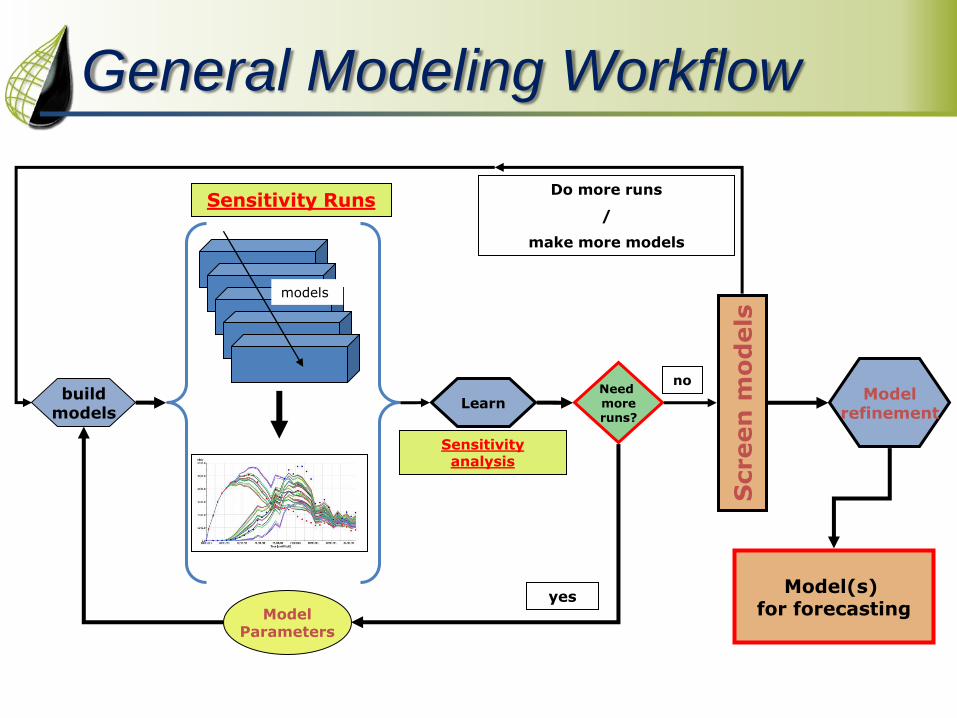
General Modeling Workflow
Need more runs?
Sensitivity Runs
Screen
mo
dels
build models
Learn
no
yes
Model refinement
Model(s) for forecasting
Do more runs
/
make more models
Model Parameters
models
Sensitivity analysis
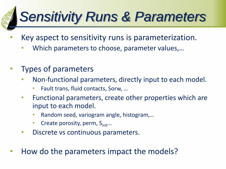
Sensitivity Runs & Parameters
• Key aspect to sensitivity runs is parameterization. • Which parameters to choose, parameter values,…
• Types of parameters • Non-functional parameters, directly input to each model.
• Fault trans, fluid contacts, Sorw, …
• Functional parameters, create other properties which are input to each model. • Random seed, variogram angle, histogram,…
• Create porosity, perm, Sinit…
• Discrete vs continuous parameters.
• How do the parameters impact the models?
Classic Sensitivity Analysis
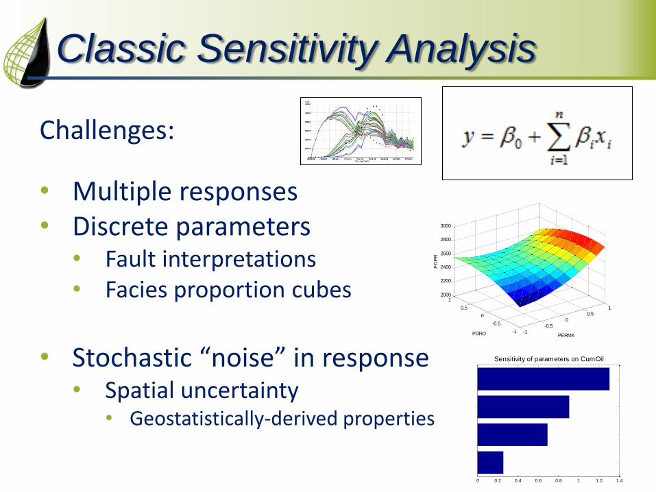
Challenges:
• Multiple responses • Discrete parameters
• Fault interpretations • Facies proportion cubes
• Stochastic “noise” in response
• Spatial uncertainty • Geostatistically-derived properties
-1
-0.5
0
0.5
1
-1
-0.5
0
0.5
12000
2200
2400
2600
2800
3000
PERMXPORO
FO
PR
0 0.2 0.4 0.6 0.8 1 1.2 1.4
1
2
3
4
Sensitivity of parameters on CumOil
Improved Screening Method
• Need method that can: • Apply to different types of parameters and different
responses.
• Identify important parameters with respect to desired response.
• Extract diverse set of parameters for uncertainty quantification.
• Compare models with respect to each other.
• Identify “best” models for HM.
• Generalized screening diagnostics needed.
Metric Space Methods for Screening
• The “distances” between a set of points defines a Metric Space (MS).
• MS methods used in internet search engines, image comparison, protein classification, etc.
• MS methods applied by Scheidt & Caers to reservoir modeling (2008, 2009).
MS Method - Key Concepts
1. Dissimilarity Distance. Measures dissimilarity between two models based upon a
distance measure.
2. Multi-Dimensional Scaling (MDS)
Translates all distances to a lower-dimensional space, separated by the distance measure.
3. Cluster Analysis Groups similar models in MDS space.
Perform sensitivity analysis and model screening using
metric space information
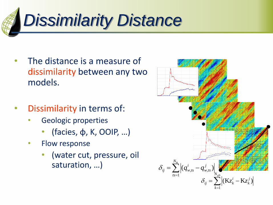
Dissimilarity Distance
• The distance is a measure of dissimilarity between any two models.
• Dissimilarity in terms of: • Geologic properties
• (facies, φ, K, OOIP, …) • Flow response
• (water cut, pressure, oil saturation, …)
1x
2x
Nx
gbN
k
j
k
i
kij zz1
)KK(
tsN
ts
j
tsw
i
tswij qq1
,, )(
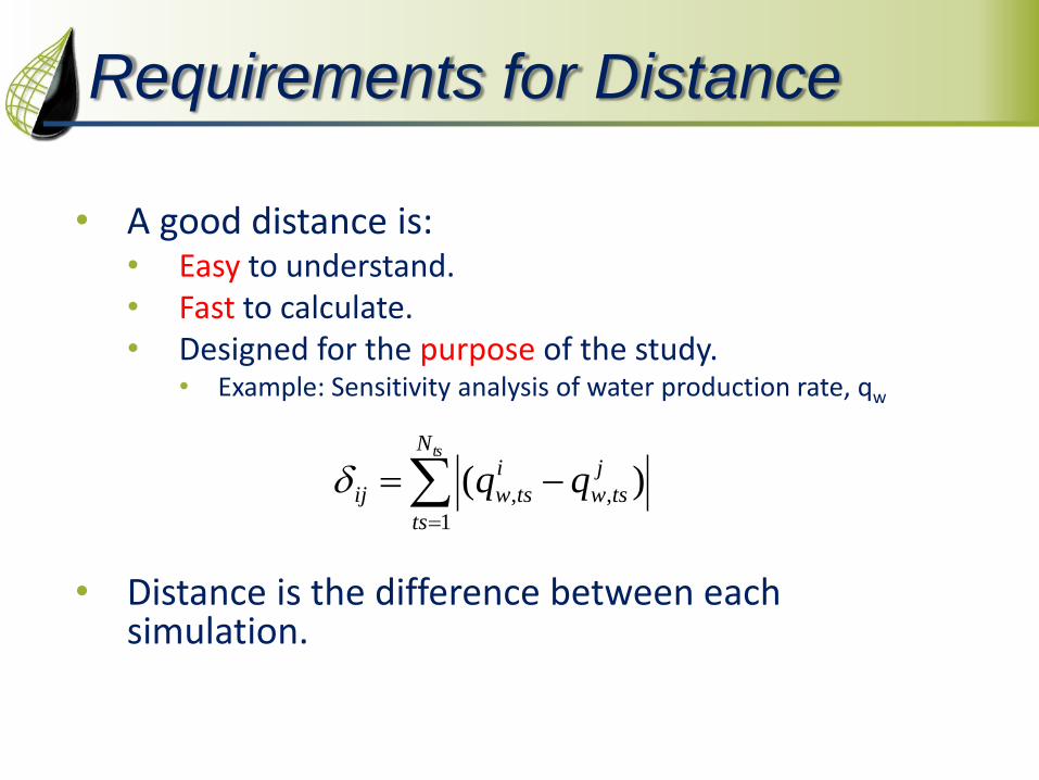
Requirements for Distance
• A good distance is: • Easy to understand. • Fast to calculate. • Designed for the purpose of the study.
• Example: Sensitivity analysis of water production rate, qw
• Distance is the difference between each
simulation.
tsN
ts
j
tsw
i
tswij qq1
,, )(
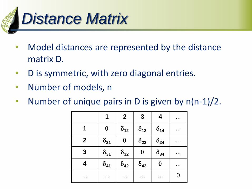
Distance Matrix
• Model distances are represented by the distance matrix D.
• D is symmetric, with zero diagonal entries.
• Number of models, n
• Number of unique pairs in D is given by n(n-1)/2.
1 2 3 4 ...
1 0 12 13 14 ...
2 21 0 23 24 ...
3 31 32 0 34 ...
4 41 42 43 0 ...
... ... ... ... ... 0
Multi-Dimensional Scaling (MDS)
• D matrix is difficult to visualize and understand.
• MDS transforms the dissimilarity distance into an approximate Euclidean distance. • Uses Eigenvalue decomposition of D.
• Display Euclidean distances in MDS plot, visual and
diagnostic tool. • Visualizes models relative to each other.
• Identifies similar models (screening)
• Visualizes model uncertainty & response sensitivity.
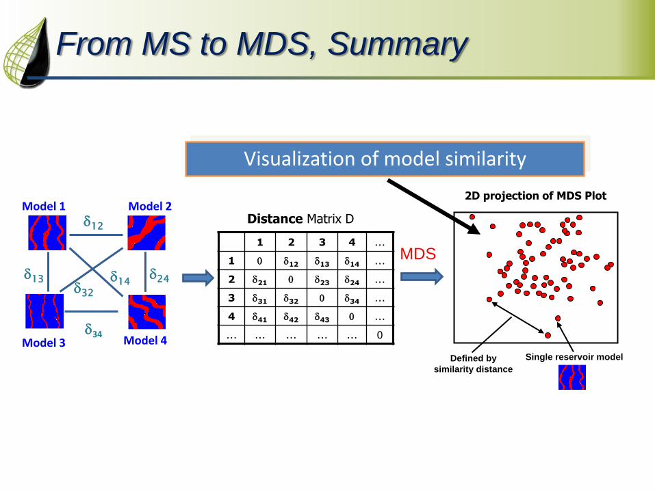
From MS to MDS, Summary
Distance Matrix D
1 2 3 4 ...
1 0 12 13 14 ...
2 21 0 23 24 ...
3 31 32 0 34 ...
4 41 42 43 0 ...
... ... ... ... ... 0
Model 1 Model 2
Model 3 Model 4
12
13 24
34
32
14
2D projection of MDS Plot
MDS
Single reservoir model Defined by
similarity distance
Visualization of model similarity
1 2 3 4 ...
1 11 12 13 14 ...
2 21 22 23 24 ...
3 31 32 33 34 ...
4 41 42 43 44 ...
... ... ... ... ... ...
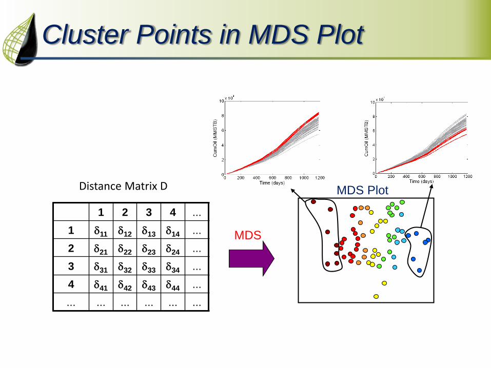
Distance Matrix D
Cluster Points in MDS Plot
MDS
MDS Plot
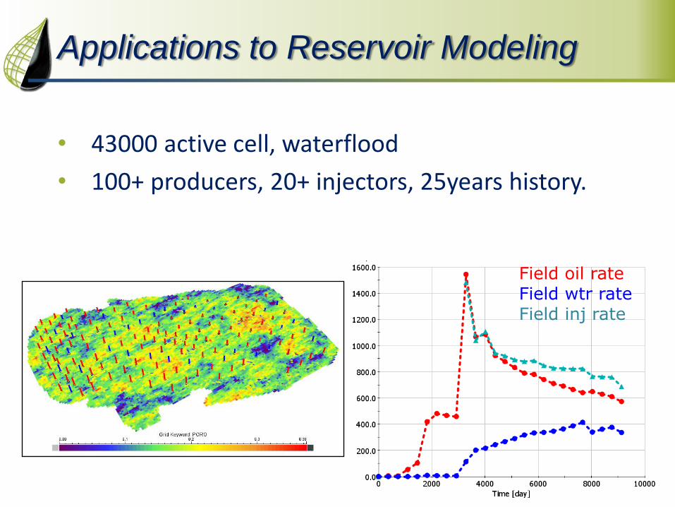
Applications to Reservoir Modeling
• 43000 active cell, waterflood
• 100+ producers, 20+ injectors, 25years history.
Field oil rate Field wtr rate Field inj rate
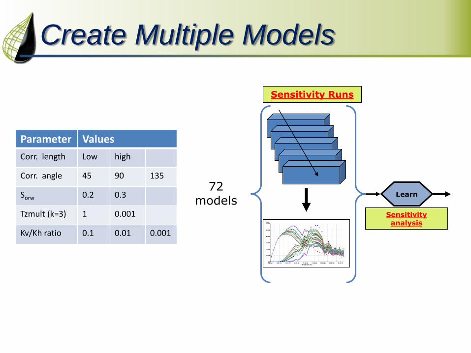
Create Multiple Models
Parameter Values
Corr. length Low high
Corr. angle 45 90 135
Sorw 0.2 0.3
Tzmult (k=3) 1 0.001
Kv/Kh ratio 0.1 0.01 0.001
Sensitivity Runs
Learn 72
models Sensitivity analysis
Static Property-based Distance Measure
• A distance based on static gridblock properties is fast to compute. No flow simulation required.
• Useful if there are many models or flow simulation per model is expensive.
• Is a static-based distance a good proxy for flow response?
• Depends on the flow response we are studying.
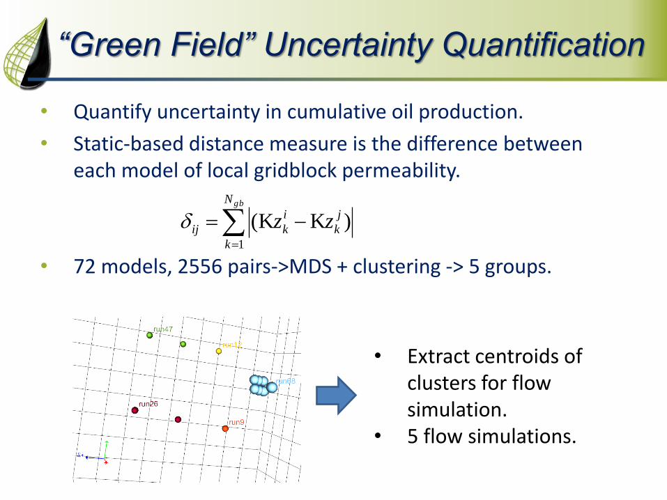
“Green Field” Uncertainty Quantification
• Quantify uncertainty in cumulative oil production.
• Static-based distance measure is the difference between each model of local gridblock permeability.
• 72 models, 2556 pairs->MDS + clustering -> 5 groups.
gbN
k
j
k
i
kij zz1
)KK(
• Extract centroids of clusters for flow simulation.
• 5 flow simulations.
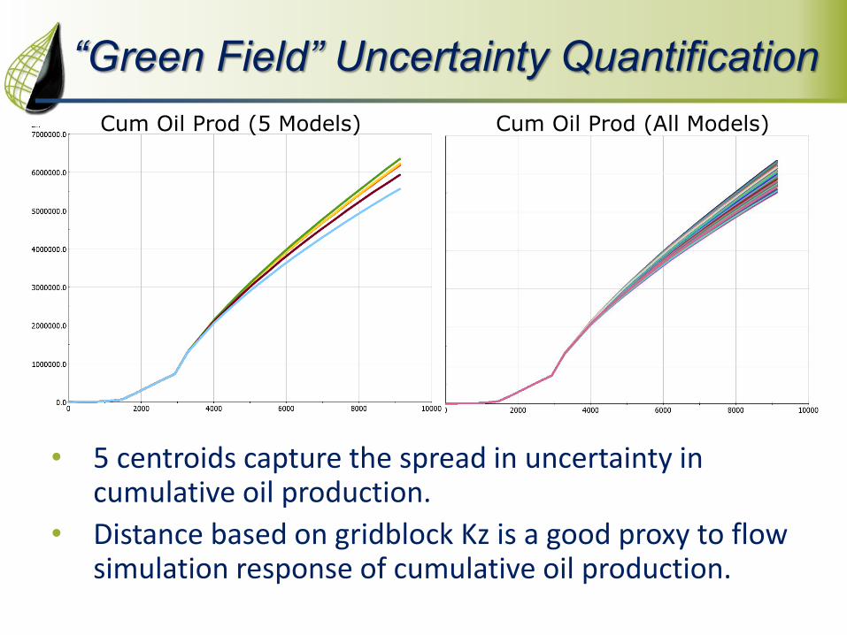
“Green Field” Uncertainty Quantification
Cum Oil Prod (5 Models) Cum Oil Prod (All Models)
• 5 centroids capture the spread in uncertainty in cumulative oil production.
• Distance based on gridblock Kz is a good proxy to flow simulation response of cumulative oil production.
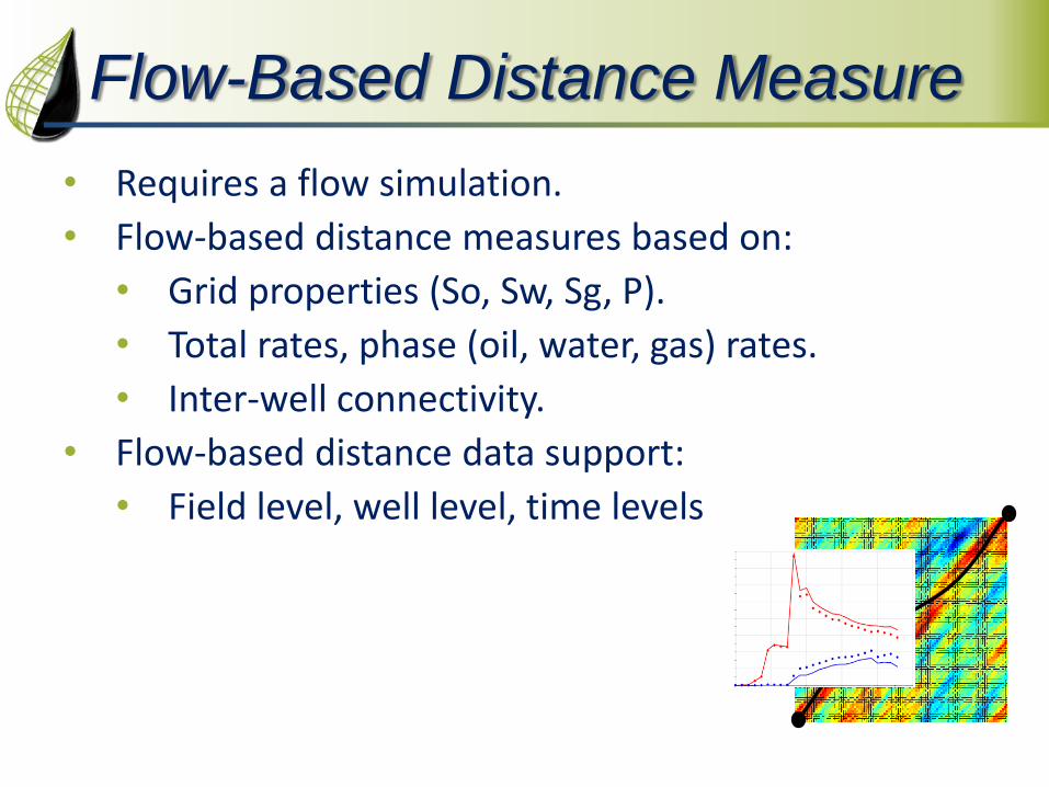
Flow-Based Distance Measure
• Requires a flow simulation.
• Flow-based distance measures based on:
• Grid properties (So, Sw, Sg, P).
• Total rates, phase (oil, water, gas) rates.
• Inter-well connectivity.
• Flow-based distance data support:
• Field level, well level, time levels
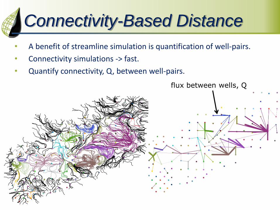
Connectivity-Based Distance
• A benefit of streamline simulation is quantification of well-pairs.
• Connectivity simulations -> fast.
• Quantify connectivity, Q, between well-pairs.
flux between wells, Q
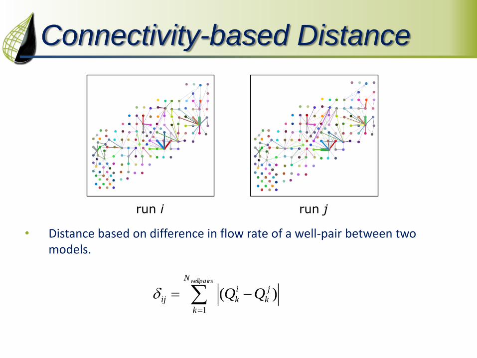
Connectivity-based Distance
wellpairsN
k
j
k
i
kij QQ1
)(
run i run j
• Distance based on difference in flow rate of a well-pair between two models.
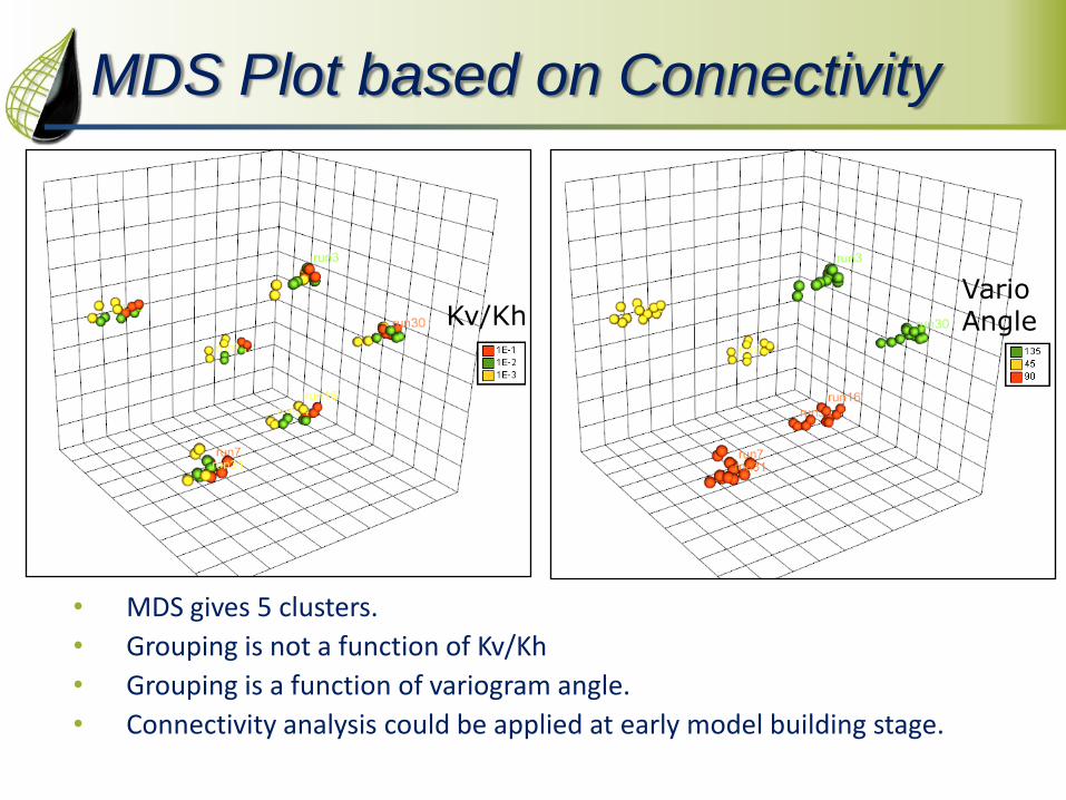
MDS Plot based on Connectivity
• MDS gives 5 clusters.
• Grouping is not a function of Kv/Kh
• Grouping is a function of variogram angle.
• Connectivity analysis could be applied at early model building stage.
Kv/Kh Vario Angle
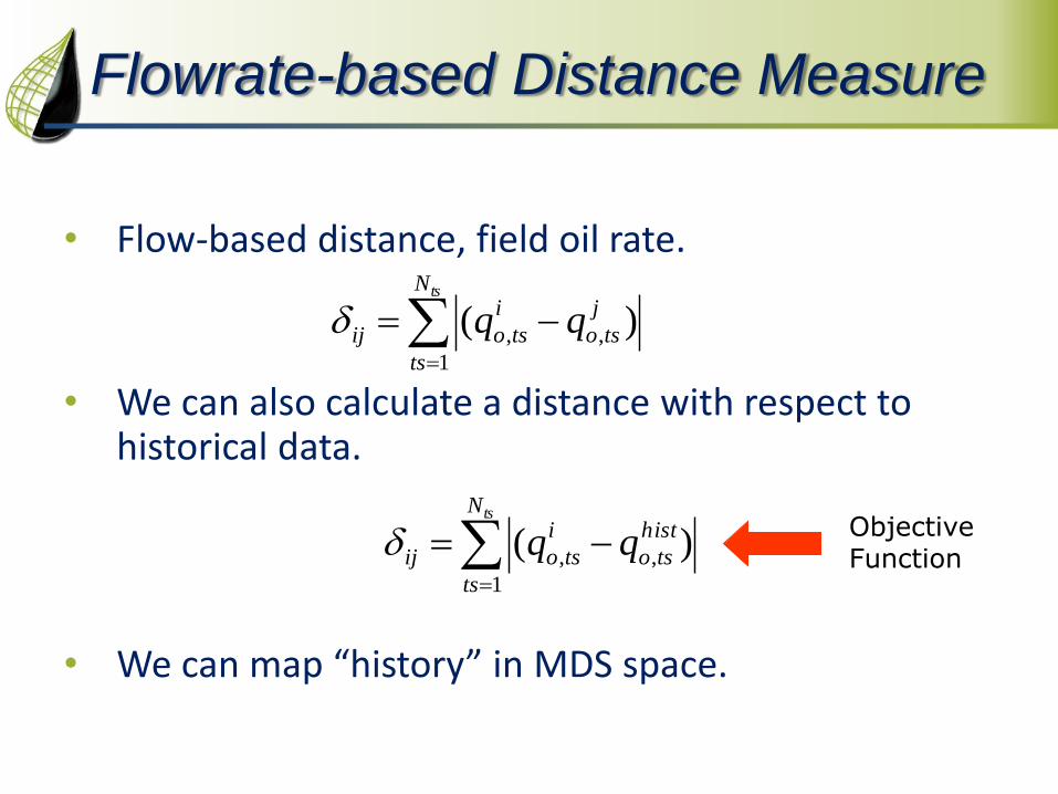
Flowrate-based Distance Measure
• Flow-based distance, field oil rate.
• We can also calculate a distance with respect to historical data.
• We can map “history” in MDS space.
Objective Function
tsN
ts
j
tso
i
tsoij qq1
,, )(
tsN
ts
hist
tso
i
tsoij qq1
,, )(
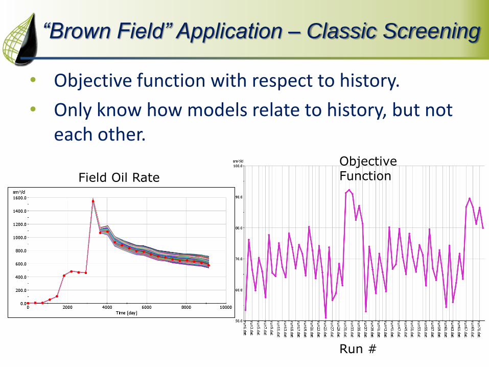
“Brown Field” Application – Classic Screening
• Objective function with respect to history.
• Only know how models relate to history, but not each other.
Objective Function Field Oil Rate
Run #
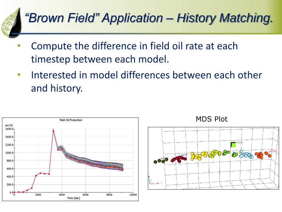
“Brown Field” Application – History Matching.
• Compute the difference in field oil rate at each timestep between each model.
• Interested in model differences between each other and history.
MDS Plot
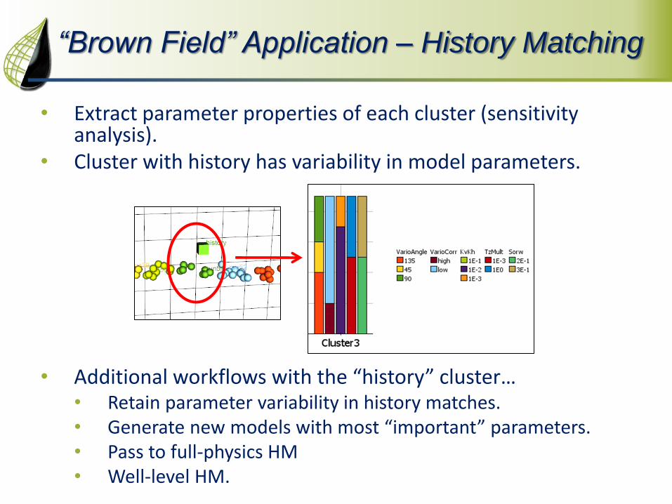
“Brown Field” Application – History Matching
• Extract parameter properties of each cluster (sensitivity analysis).
• Cluster with history has variability in model parameters.
• Additional workflows with the “history” cluster…
• Retain parameter variability in history matches. • Generate new models with most “important” parameters. • Pass to full-physics HM • Well-level HM.
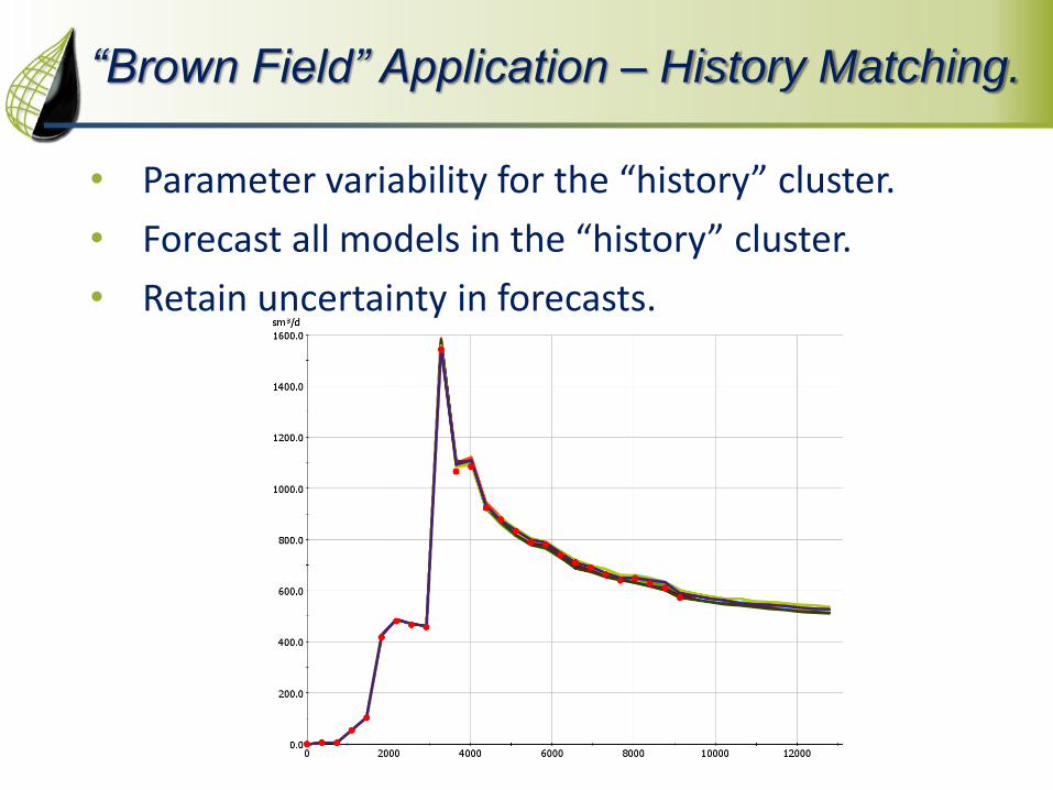
“Brown Field” Application – History Matching.
• Parameter variability for the “history” cluster.
• Forecast all models in the “history” cluster.
• Retain uncertainty in forecasts.
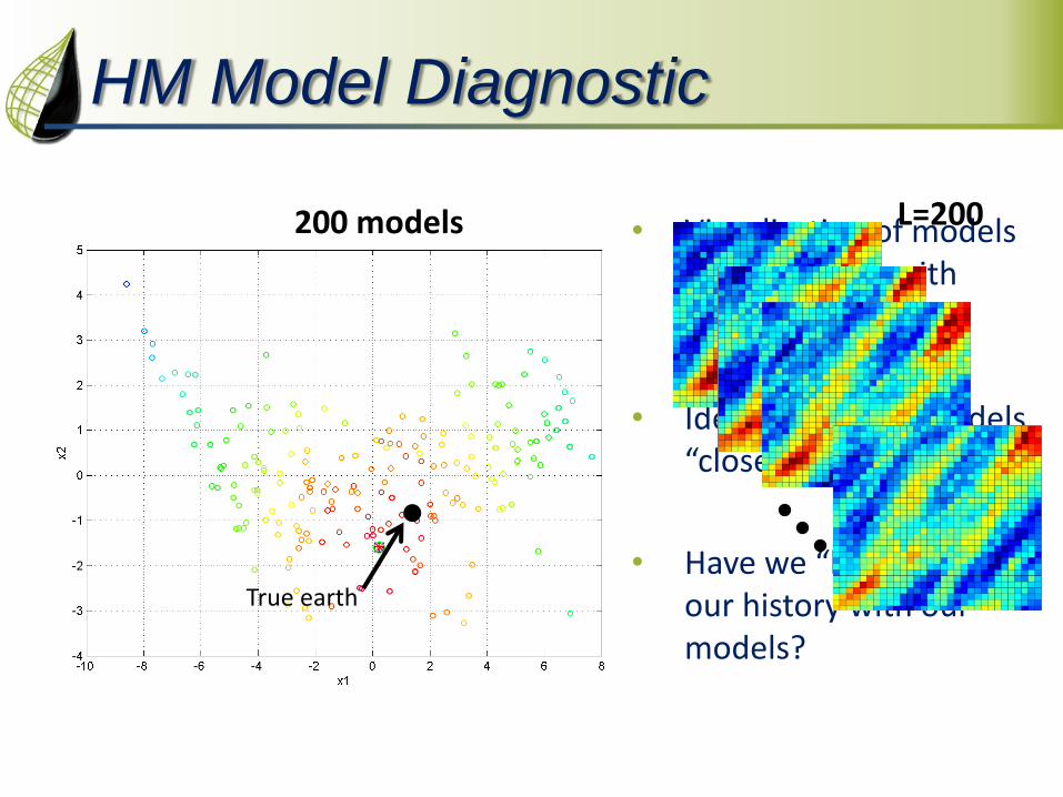
HM Model Diagnostic
• Visualization of models & comparison with history
• Identification of models “close” to history
• Have we “bracketed” our history with our models?
200 models
True earth
L=200
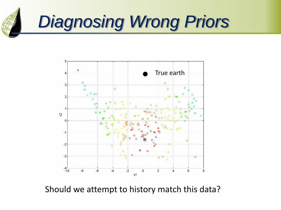
Diagnosing Wrong Priors
True earth
Should we attempt to history match this data?
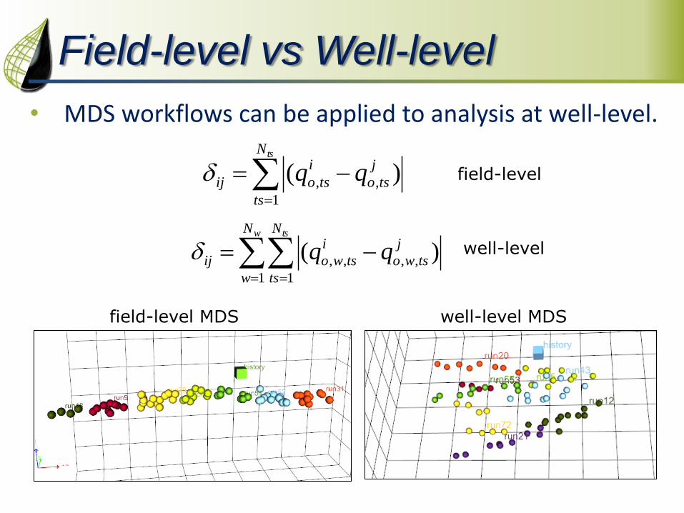
Field-level vs Well-level
• MDS workflows can be applied to analysis at well-level.
w tsN
w
N
ts
j
tswo
i
tswoij qq1 1
,,,, )(
tsN
ts
j
tso
i
tsoij qq1
,, )( field-level
well-level
field-level MDS well-level MDS
Conclusions
• Introduce Metric Space and MDS as a new method to screen models.
• A general method based on differences that can work with any parameter type any model response.
• Compare models to history and to each other. • Quantify and retain diversity within the HM. • Guide which parameters are important to vary in the HM. • Diagnose wrong priors, ensemble close/far from history.
• Cluster analysis quantifies: • Impact of parameters on each cluster. • Diversity in each cluster or diversity of the centroids. • Uncertainty in forecasts and history matches.
• Software allows easy application of MS methods to reservoir uncertainty workflows.