Using Hyperbolic Cross Approximation to measure and compensate

JMLR: Workshop and Conference Proceedings 29:435–450, 2013 ACML 2013

Using Hyperbolic Cross Approximationto measure and compensate Covariate Shift

Thomas Vanck [email protected] fur Mathematik, Technische Universitat Berlin, Berlin

Jochen Garcke [email protected]

Institut fur Numerische Simulation, Universitat Bonn and Fraunhofer SCAI, Sankt Augustin

Editor: Cheng Soon Ong and Tu Bao Ho

Abstract

The concept of covariate shift in supervised data analysis describes a difference betweenthe training and test distribution while the conditional distribution remains the same. Toimprove the prediction performance one can address such a change by using individualweights for each training datapoint, which emphasizes the training points close to the testdata set so that these get a higher significance. We propose a new method for calculatingsuch weights by minimizing a Fourier series approximation of distance measures, in partic-ular we consider the total variation distance, the Euclidean distance and Kullback-Leiblerdivergence. To be able to use the Fourier approach for higher dimensional data, we employthe so-called hyperbolic cross approximation. Results show that the new approach cancompete with the latest methods and that on real life data an improved performance canbe obtained.

Keywords: Covariate Shift, Fourier Series Approximation, Hyperbolic Cross, Curse ofDimensionality

1. Introduction

In a standard machine learning setting it is assumed that the test data is essentially drawnfrom the same distribution as the training data, i.e.

p(x, y) = p(y|x)p(x) and p(x) = ptr(x) = pte(x).

In practice, however, the training distribution ptr can differ significantly from the testdistribution pte, while the functional relationship p(y|x) remains the same. Such a situation,where ptr(x) 6= pte(x), is known as covariate shift and can arise from several circumstances.For example, in non stationary cases the distribution of the covariate might change overtime. In parameter optimization scenarios a good extrapolation into before unseen regionsof the parameter domain is often needed. Or the actual (geographical) location of somemeasurements may have an impact, as is the case for the earthquake dataset considered inthis paper.

The covariate shift is the result of some kind of bias that influences the input variablesx. Hence, the test datapoints are drawn from regions that are not covered, or by far notas densely, by the training samples. Therefore, a model learned on the training data mightnot be well suited for prediction of the test labels. To rectify this problem one can put

c© 2013 T. Vanck & J. Garcke.

Vanck Garcke

more weight on training datapoints that lie close to the test data Xte, assuming that thesebetter represent the structure of the test data. Note that in supervised learning such asituation where, besides the training data, additional samples are available for whose onlythe locations x are given is known as semi-supervised learning (Chapelle et al., 2006).

A common approach to handle such a situation is importance sampling. If one knew thetraining and test distribution one could give weights directly by calculating the importancesampling weight function

w(x) =pte(x)

ptr(x). (1)

Since this information is unavailable it is necessary to estimate these weights.Several methods have recently been proposed for inferring individual weights for each

training datapoint. Bickel et al. (2009) proposed a kernel logistic regression classifier forcovariate shift. Another method is the so-called Kernel Mean Matching (KMM) (Huanget al., 2007) algorithm, where all moments in the original space are mean matched. KLIEP(Kullback Leibler Importance Estimation Procedure) has been put forward by Sugiyamaet al. (2008), it minimizes the Kullback Leibler divergence for retrieving optimal weights.Furthermore this procedure was extended by Tsuboi et al. (2009) to large-scale problems.Least-squares importance fitting (uLSIF) is another recent method which was stated byKanamori et al. (2009). For recent surveys on the state of the art on covariate shift aswell as the more general dataset shift see Quionero-Candela et al. (2009); Sugiyama andKawanabe (2012); Moreno-Torres et al. (2012). All these methods assume some overlap ofthe samples from the two distributions ptr and pte. In cases where the training and testdistribution have nothing in common, i.e. the samples are disjunct, it will not be possibleto derive reasonable information for the calculation of the weights just from the sampleswithout strong additional assumptions about the type of distributions involved.

In this paper we propose a new approach for estimating the weights. We use a Fourierapproximation of a distance measure to estimate the divergence of distributions. In a cer-tain sense the measuring of the divergence becomes less data centered since an explicitdiscretization of the underlying error function is involved. The Fourier based approach doesnot depend on a specific distance measure, nor on a specific point set for empirically esti-mating the distance measure. We will minimize the total variation distance, the Kullback-Leibler divergence and the Euclidean distance. The training and test data are then usedduring the estimation of the Fourier coefficents of the resulting distance function. It can beseen that the resulting constrained optimization problem is convex and can be solved withstandard methods. Furthermore, we give some evidence that under certain circumstancesthe application of the Fourier series will lead to a better weight estimation in comparison toother approaches. Note that a Fourier series approximation for high dimensional functionsquickly runs into the curse of dimensionality due to the exponential growth of the number ofcoefficients. To overcome this we will apply the hyperbolic cross approach (Babenko, 1960;Smolyak, 1963; Knapek, 2000) which enables us to apply a Fourier series approximation tohigh dimensional functions by simultaneously keeping an acceptable degree of accuracy.

The paper is structured in the following way: In section 2 we introduce our new methodand section 3 gives insights why the new method is beneficial. The extension to higherdimensional data based on the hyperbolic cross approximation is given in section 4. Finally,

436

Hyperbolic Cross Approximation to measure and compensate Covariate Shift

sections 5 and 6 state the employed weighted regression and classification algorithms, theexperimental setup and the results obtained on diverse datasets.

2. New Fourier Based Approach

We will now motivate and derive our new approach for the calculation of importance weightsfor the training data. Mathematically speaking we would like to minimize the distance ofthe test distribution pte and the training distribution ptr which is reweighted by w

minwD(pte(x)‖w(x)ptr(x)). (2)

Expression (2) can be minimized using different distance measures. Typically one choosesdivergence measures from the classes of Csiszar or Bregman divergences, which are thenempirically evaluated on some points {xi}Ni=1. Here one often uses training {xtri }

Ntri=1 or test

datapoints {xtei }Ntei=1 for the evaluation points in the distance estimation.

Let us consider the class of Csiszar divergences, defined as Dh(p||q) =∑N

i=1 qih(piqi ),where h is a real-valued convex function satisfying h(1) = 0 and we define pi := p(xi),qi := q(xi). Different h yield different divergences. For the following exposition we seth(u) = |u− 1| and considering that qi > 0 ∀i we get the total variation distance

Dh(p||q) =

N∑i=1

qi

∣∣∣∣piqi − 1

∣∣∣∣ =

N∑i=1

|pi − qi|. (3)

Substituting (3) into (2) we get

minwDh(pte(x)‖w(x)ptr(x)) = min

w

N∑i=1

|pte(xi)− w(xi)ptr(xi)|. (4)

Note that in contrast to many other approaches, our methodology does not depend on aspecific choice of the points {xi}Ni=1 and we are able to use any point set in the distanceestimation (4). Nevertheless, for the sake of comparison with other approaches, we useeither training or test datapoints in (4) for our experiments in Section 6.

Observe that the Fourier based approach which we will describe in the following can bedirectly applied to different divergence measures. For example, a generalisation of the total

variation distance, the so called Matsusita or Hellinger distance, i.e. h(u) = |uγ−1|1γ which

yields∑N

i=1 |pγi −q

γi |

1γ , could be used. We later state our approach with the Kullback-Leibler

divergence and the Euclidean distance, respectively.

2.1. Choice of the Weight Function

The optimization problem (2) states the problem of finding an optimal weight function w(x)which minimizes the distance of the two functions pte and w · ptr. The exact solution wouldbe the quotient of the density functions, i.e. w(x) = pte(x)

ptr(x), which of course is not available.

Therefore one can only compute an approximation w of w. For the discrete representation

437

Vanck Garcke

of w we will, as in Sugiyama et al. (2008); Kanamori et al. (2009), use a linear combinationof Gaussian kernels

w(x, α) =

Z∑j=1

αj exp

(−‖x− ζj‖

2

2σ2

). (5)

It is comprised of Z ∈ N exponential functions each of which centered at a ζj . In ourexperiments we will use the test data as the center points ζj , as in Sugiyama et al. (2008);Kanamori et al. (2009). There it is argued that using test points as the Gaussian centersis preferable, since kernels may be needed where the target function w(x) is large, whichis the case where the training density ptr(x) is small and the test density pte(x) is large.Note that the ratio (1) implies positive weights, which is the case for any x and any α ≥ 0in w(x, α). Other weight function representations are possible, but to concentrate on theeffect of the new Fourier based distance estimation and to be able to better compare withother approaches we consider the linear combination of Gaussian kernels in this work.

Inserting (5) into (4) now yields

minwDh(pte(x)‖w(x)ptr(x)) ≈ min

α≥0

N∑n=1

|pte(xn)− w(xn, α)ptr(xn)|. (6)

Note that this minimization problem still employs the probability densities directly. In thenext step we will now approximate this term using a Fourier series approximation.

2.2. Fourier Series Approximation

Our new approach makes use of Fourier series approximation, with which we discretize theemployed distance measure, taking a more function centric view as opposed to the morecommon data centric view. Section 3 provides a discussion of the advantages of this newapproach, while section 4 explains the case of more than one dimension.

Let now f be a continuous periodic function with period T > 0 and partially continuousderivatives; then the Fourier series is defined as

f(x) =∞∑

k=−∞cke

i 2πkTx, ck =

1

T

∫ t+T

tf(x)e−i

2πkTxdx, (7)

where i denotes the imaginary unit and t ∈ R is an arbitrary point. For a suitably smoothfunction we can approximate this expression in a controlled fashion by a truncated Fourierseries with |k| ≤ K

f(x) ≈K∑

k=−Kcke

i 2πkTx, (8)

where K is chosen to achieve a given error, see section 4 for more details on the approxi-mation properties.

We consider now the error function between the two densities

f(x) := pte(x)− w(xn, α)ptr(x).

438


We assume that the given data is bounded to a certain region, i.e. Xtr∪Xte ⊂ [t, t+T ] ⊂ R,for suitable chosen t, T . Assuming periodicity of f on that interval implies that we makethe same small error on the boundary, which is our aim in the minimization. Furthermore,the interesting region is the inner part where the two samples overlap, near the boundary ofthe domain the densities will be small in any case, which, if necessary, can even be enforcedby having a reasonable gap between the given data and the actual boundary of the interval.Therefore we can reasonably assume a continuous periodic extension of the Fourier seriesof f and avoid the Gibbs phenomen, i.e. potential overshoots on the boundary, in practice.

We now apply the Fourier series approximation to our problem (6). Due to its definitionwe can replace the densities by the empirical samples in the formula (7) for the coefficientsck after splitting the integral into two

ck(α) =1

T

∫ t+T

tpte(x)e−i

2πkTxdx− 1

T

∫ t+T

tw(x, α)ptr(x)e−i

2πkTxdx (9)

≈ 1

TNte

Nte∑l=1

e−i2πkTxtel − 1

TNtr

Ntr∑l=1

w(xtrl , α)e−i2πkTxtrl . (10)

In the last part of this equation we approximate the two integrals by taking the empiricalexpectation based on the training and test data, respectively. Therefore, we no longerexplicitly need the unknown densities but use their known samples.

2.3. Optimization Problem

The original problem (2) is about finding an appropriate weight function. Employing (5)for given parameter σ and center points (ζj)

Zj=1 and using the Fourier approximation (8)

for a suitably chosen K we obtain the following optimization problem

minα≥0

N∑n=1

|pte(xn)− w(xn, α)ptr(xn)| ≈ minα≥0

N∑n=1

∣∣∣∣∣K∑

k=−Kck(α)ei

2πkTxn

∣∣∣∣∣ . (11)

Due to the linearity of this problem we can express it in matrix notation. Defining thematrix A ∈ RN×Z as A = [A1| . . . |AN ], where the An ∈ RZ are column vectors comprised,after inserting (5) for w, of the entries

(An)j =

K∑k=−K

1

TNtr

Ntr∑l=1

e−‖xtrl −ζj‖

2

2σ2 e−i2πkTxtrl ei

2πkTxn , j = 1, . . . , Z.

Additionally we get a vector b ∈ RN , defined as

bn =K∑

k=−K

Nte∑l=1

1

TNtee−i

2πkTxtel ei

2πkTxn , n = 1, . . . , N.

The problem (11) can now be stated as a L1 minimization problem with side conditions ina compact notation by employing A and b

minα≥0‖Aα− b‖1 .

439

Vanck Garcke

2.4. Normalization Constraints

It is possible that a solution to the optimization problem (11) might not yield appropriateweights. Often only a small fraction of αs will be larger than zero, which leads to a situationwhere only a few training datapoints will get importance. To compensate, we employ anapproach which is similar to the one introduced in Sugiyama et al. (2008). From (1) we havepte(x) = w(x)ptr(x), and taking the integral on both sides yields the natural side condition

1 =

∫pte(x)dx =

∫w(x)ptr(x)dx ≈ 1

Ntr

Ntr∑n=1

w(xtrn , α),

again using the empirical samples and the approximation w. We augment (11) and get anew constrained optimization problem1

minα≥0‖Aα− b‖1 s.t.

1

Ntr

Ntr∑n=1

w(xtrn , α) = 1. (12)

2.5. Kullback-Leibler Divergence

An advantage of the Fourier approach is that it can directly be applied to different divergencemeasures. To demonstrate this flexibility we will use as a second Csiszar divergence theKullback-Leibler divergence, which also allows us to compare with KLIEP (Sugiyama et al.,2008). Roughly following the KLIEP derivation gives

KL(pte‖wptr) =N∑n=1

pte(xn) log

(pte(xn)

w(xn)ptr(xn)

)

=

N∑n=1

pte(xn) log

(pte(xn)

ptr(xn)

)−

N∑n=1

pte(xn) log (w(xn)) .

Since the first part does not depend on w, it suffices to minimize

arg minw

KL(pte‖wptr) ≈ arg minα≥0

−N∑n=1

pte(xn) log (w(xn, α)) , (13)

where we employ the approximation w of w. Using the same normalization approach asabove, the final optimization problem becomes

minα≥0

N∑n=1

K∑k=−K

ck(α)ei2πkTxn s.t.

Ntr∑n=1

w(xtrn , α)

Ntr= 1, (14)

where

ck(α) =1

T

∫ t+T

t−pte(x) log (w(x, α)) e−i

2πkTxdx ≈ −1

TNte

Nte∑l=1

log(w(xtel , α)

)e−i

2πkTxtel .

1. We used the YALL1 Basic solver from http://yall1.blogs.rice.edu/.

440


Although the approach is very similar to the one suggested by Sugiyama et al. (2008), weget a different optimization problem2 due to the Fourier approximation and also estimatethe divergence in a different fashion. Note that the KL divergence is a special case of thegeneralized KL divergence or I-Divergence which is from the class of Bregman divergences.The Fourier approach could also be applied for these.

2.6. Euclidean Distance

The third distance measure that we will investigate is the Euclidean distance, which belongsto the class of Bregman divergences, and was also used for uLSIF (Kanamori et al., 2009).Bregman divergences are defined by

Dφ(p‖q) = φ(p)− φ(q)− φ′(q)(p− q),

where φ is a strictly convex real-valued function and φ′(q) denotes the derivative withrespect to q. Setting φ(·) = || · ||22 we get

D||·||22(p‖q) = ||p||22 − ||q||22 − 2q(p− q) = ||p− q||22.

Employing the data, the weight function w and applying the Fourier approximation we getthe following optimization problem:

minα≥0‖Aα− b‖22 s.t.

1

Ntr

Ntr∑n=1

w(xtrn , α) = 1, (15)

where A and b are defined as in (2.3).

3. Benefits of the Fourier Approximation

The following illustrative example shows the behavior of our approach. The weight functionw is chosen according to (5). For the sake of comparison, we use the Kullback-Leiblerdivergence and the Euclidean distance here.

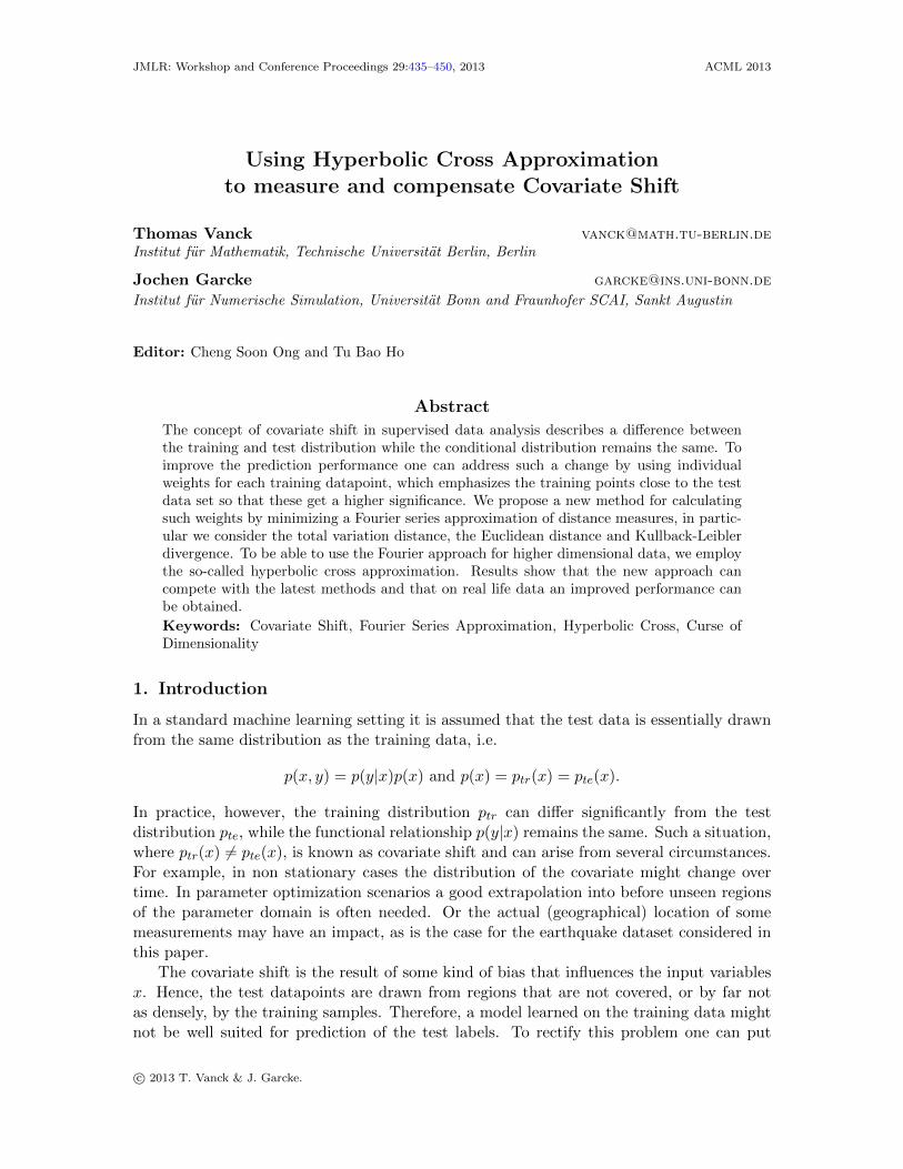
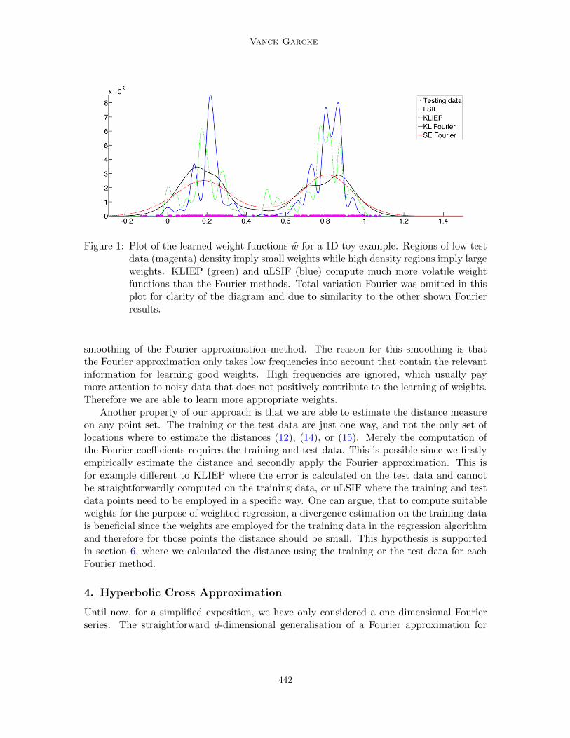
We note that by estimating the divergence measure using the Fourier approximationwe achieve a smoothing of the weights. This becomes especially useful when a small band-width parameter σ is chosen for the weight function w. As Figure 1 illustrates the weightslearned by the Fourier methods are much smoother and stable than the weights learnedby KLIEP (Sugiyama et al., 2008) or uLSIF (Kanamori et al., 2009) which involve a muchhigher volatility. In the case of Figure 1 we applied the bandwidth parameter σ that waschosen by KLIEP also to the Fourier methods for the sake of comparison. Although we didnot apply our method of parameter selection, the Fourier methods outperform KLIEP, inthe sense of a less volatile weight function. Note that the parameters for uLSIF have beendetermined by its own parameter estimation method.

The comparison of KLIEP and KL-Fourier is of special interest here because this is adirect comparison of two very similar methods which clearly shows the advantages of the

2. We here used IPOpt from https://projects.coin-or.org/Ipopt, which is also used for the Euclidean dis-tance.

441

Vanck Garcke

Figure 1: Plot of the learned weight functions w for a 1D toy example. Regions of low testdata (magenta) density imply small weights while high density regions imply largeweights. KLIEP (green) and uLSIF (blue) compute much more volatile weightfunctions than the Fourier methods. Total variation Fourier was omitted in thisplot for clarity of the diagram and due to similarity to the other shown Fourierresults.

smoothing of the Fourier approximation method. The reason for this smoothing is thatthe Fourier approximation only takes low frequencies into account that contain the relevantinformation for learning good weights. High frequencies are ignored, which usually paymore attention to noisy data that does not positively contribute to the learning of weights.Therefore we are able to learn more appropriate weights.

Another property of our approach is that we are able to estimate the distance measureon any point set. The training or the test data are just one way, and not the only set oflocations where to estimate the distances (12), (14), or (15). Merely the computation ofthe Fourier coefficients requires the training and test data. This is possible since we firstlyempirically estimate the distance and secondly apply the Fourier approximation. This isfor example different to KLIEP where the error is calculated on the test data and cannotbe straightforwardly computed on the training data, or uLSIF where the training and testdata points need to be employed in a specific way. One can argue, that to compute suitableweights for the purpose of weighted regression, a divergence estimation on the training datais beneficial since the weights are employed for the training data in the regression algorithmand therefore for those points the distance should be small. This hypothesis is supportedin section 6, where we calculated the distance using the training or the test data for eachFourier method.

4. Hyperbolic Cross Approximation

Until now, for a simplified exposition, we have only considered a one dimensional Fourierseries. The straightforward d-dimensional generalisation of a Fourier approximation for

442


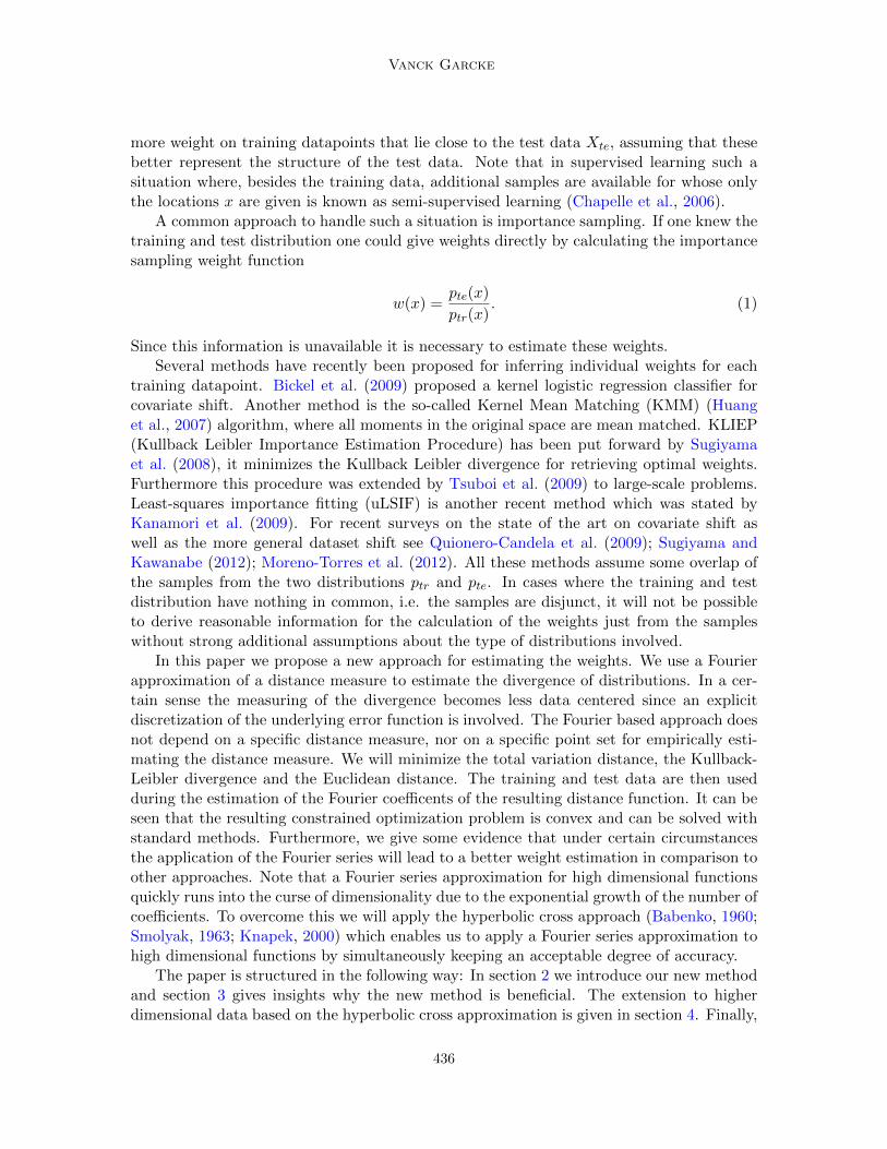
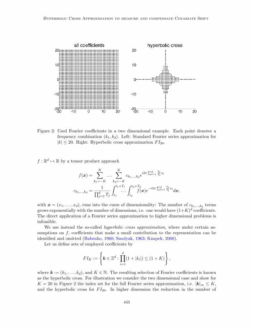
Figure 2: Used Fourier coefficients in a two dimensional example. Each point denotes afrequency combination (k1, k2). Left: Standard Fourier series approximation for|k| ≤ 20. Right: Hyperbolic cross approximation FI20.

f : Rd 7→ R by a tensor product approach

f(x) =

K∑k1=−K

. . .

K∑kd=−K

ck1,...,kdei2π

∑dl=1

klTlxl

ck1,...,kd =1∏d

j=1 Tj

∫ t1+T1

t1

. . .

∫ td+Td

td

f(x)e−i2π

∑dl=1

klTlxldx,

with x = (x1, . . . , xd), runs into the curse of dimensionality: The number of ck1,...,kd termsgrows exponentially with the number of dimensions, i.e. one would have (1+K)d coefficients.The direct application of a Fourier series approximation to higher dimensional problems isinfeasible.

We use instead the so-called hyperbolic cross approximation, where under certain as-sumptions on f , coefficients that make a small contribution to the representation can beidentified and omitted (Babenko, 1960; Smolyak, 1963; Knapek, 2000).

Let us define sets of employed coefficients by

FIK :=

{k ∈ Zd :

d∏i=1

(1 + |ki|) ≤ (1 +K)

},

where k := (k1, . . . , kd), and K ∈ N. The resulting selection of Fourier coefficients is knownas the hyperbolic cross. For illustration we consider the two dimensional case and show forK = 20 in Figure 2 the index set for the full Fourier series approximation, i.e. |k|∞ ≤ K,and the hyperbolic cross for FI20. In higher dimension the reduction in the number of

443

Vanck Garcke

Fourier coefficients will be even stronger noticable and is of several orders of magnitude,going from an impossible computation for the full Fourier approximation of degree K to apossible one using the hyperbolic cross approximation based on the set FIK .

Looking at the number of coefficients in FIK the advantage in higher dimensions be-comes clear:

|FIK | = O(

(1 +K) (log(1 +K))d−1),

instead of (1 +K)d for the standard Fourier approximation, see e.g. Zung (1983); Knapek(2000).

To consider the approximation properties of the hyperbolic cross Fourier approximationwe need to introduce generalisations of Sobolev spaces. For −∞ < s <∞ we define

Hsmix(Td) :=

f(x) =∑k∈Zd

ckeikx : ‖f(x)‖Hsmix <∞

‖f(x)‖2Hsmix :=

∑k∈Zd

d∏i=1

(1 + |ki|)2s|ck|2,

where Td := [0, 1]d is the n-dimensional torus which is the same as the n-dimensionalcube where opposite faces are identified. Therefore the space Hsmix is comprised of allfunctions whose Fourier coefficients ck decay sufficiently fast in the prescribed manner.The space Hsmix is called Sobolev space with dominating mixed smoothness. Note that

Hsmix ⊂ Hs ⊂ Hs/dmix for s ≥ 0 and that Hsmix(Td) = Hs(T1) ⊗ · · · ⊗ Hs(T1), where Hs(T1)

is the standard Sobolev space.We now can state the approximation properties (proof e.g. in Knapek (2000))

Lemma 1 Let t ∈ N, t < s, s ≥ 0, u ∈ Hsmix, f(x) =∑

k ckeikx and fK(x) =

∑k∈FIK cke

ikx,then it holds that

‖f − fK‖Ht ≤ (1 +K)t−s‖f‖Hsmix .

Using a hyperbolic cross we achieve for f ∈ Hsmix the same order of approximation as thestandard Fourier approximation. However, the number of coefficients is significantly reduced

from O(1 +K)d to O(

(1 +K) (log(1 +K))d−1)

, the use of a Fourier series approximation

in higher dimensions becomes feasible.A question is if we can expect that p(x) − w(x)q(x) ∈ Hsmix, which resolves to the

question of the smoothness of p and q, since w is sufficiently smooth by definition. This is aproblem-specific question and in particular depends on the unknown quantities p and q, soone can neither answer this in general, nor for a specific data set a priori. But we can giveindications that the assumption p, q ∈ Hsmix is warranted, if one expects reasonably smoothprobability distributions at all. Firstly, let us note that the mixed Sobolev spaces havean intrinsic tensor product structure with distinguished dimensions, each of which we canrelate to a specific attribute of the data set in its d-dimensional domain. This is in contrastto the standard Sobolev space Hs which only considers isotropic smoothness and has nodistinguished dimensions, e.g. the coordinate system could be rotated without changing the

444


function space. Secondly, note that the spaces Hsmix are the underlying function spaces forregression and classification approaches based on sparse grids, whose very good empiricalperformance was shown in recent years (Garcke, 2006; Pfluger, 2010).

5. Weighted Support Vector Regression (WSVR)

The calculated weights assign each training datapoint an amount of importance. High val-ues denote important datapoints, whereas low values stand for less important datapoints.Classification and regression methods need to incorporate this information so that the pre-diction in regions of heavily weighted training datapoints is more accurate. To make useof this weighting, it is necessary to modify classification and regression methods such thatthey can employ a weight for each given training datapoint. A modified support vectormachine for classification can be found in Huang et al. (2007).

Analogously, we state for regression problems a modified version of a support vectorregression (SVR) problem

minθ,b,ξ,ξ∗

1

2‖θ‖2 + C

N∑n=1

w(xn)(ξn + ξ∗n)

subject to: yn − θtφ(xn)− b ≤ ε+ ξn ξn ≥ 0

θtφ(xn) + b− yn ≤ ε+ ξ∗n ξ∗n ≥ 0.

Here θ and b denote the model parameters and w(xn) are the estimated importance weights.For each datapoint the slack variable ξ and ξ∗ is multiplied by w(xn). This implies highervalues for large weights and lower values for small weights respectively. Therefore the slackat datapoints with large weights will tend to be lower than those multiplied by small weights,thus causing a lower tolerance to errors on important datapoints. The dual version is

maxa,a∗

yt(a− a∗)−εN∑n=1

(an + a∗n)− 1

2(a− a∗)tκ(a− a∗)

subject to: 0 ≤ a ≤ w(xn)C a ≥ 0

0 ≤ a∗ ≤ w(xn)C a∗ ≥ 0

where κ is the empirical kernel map. We will use the Gaussian kernel in the following.

6. Experiments

In the experimental section we are going to show that the new approach can compete withcurrent methods for compensating the covariate shift. First we compare the Fourier basedapproach, where the distance is estimated either on the training (Tr) or the test data (Te), toother methods on some benchmark datasets, and then show results on a real world dataset.We use the total variation distance (TV), the Kullback-Leibler divergence (KL), and thesquared Euclidean distance (SE).

445

Vanck Garcke

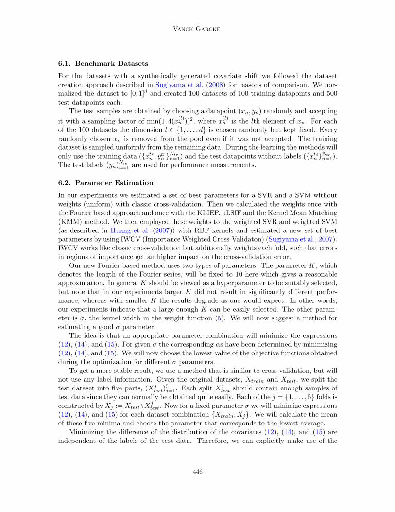
6.1. Benchmark Datasets

For the datasets with a synthetically generated covariate shift we followed the datasetcreation approach described in Sugiyama et al. (2008) for reasons of comparison. We nor-malized the dataset to [0, 1]d and created 100 datasets of 100 training datapoints and 500test datapoints each.

The test samples are obtained by choosing a datapoint (xn, yn) randomly and accepting

it with a sampling factor of min(1, 4(x(l)n ))2, where x

(l)n is the lth element of xn. For each

of the 100 datasets the dimension l ∈ {1, . . . , d} is chosen randomly but kept fixed. Everyrandomly chosen xn is removed from the pool even if it was not accepted. The trainingdataset is sampled uniformly from the remaining data. During the learning the methods willonly use the training data ({xtrn , ytrn }

Ntrn=1) and the test datapoints without labels ({xten }

Nten=1).

The test labels (yn)Nten=1 are used for performance measurements.

6.2. Parameter Estimation

In our experiments we estimated a set of best parameters for a SVR and a SVM withoutweights (uniform) with classic cross-validation. Then we calculated the weights once withthe Fourier based approach and once with the KLIEP, uLSIF and the Kernel Mean Matching(KMM) method. We then employed these weights to the weighted SVR and weighted SVM(as described in Huang et al. (2007)) with RBF kernels and estimated a new set of bestparameters by using IWCV (Importance Weighted Cross-Validaton) (Sugiyama et al., 2007).IWCV works like classic cross-validation but additionally weights each fold, such that errorsin regions of importance get an higher impact on the cross-validation error.

Our new Fourier based method uses two types of parameters. The parameter K, whichdenotes the length of the Fourier series, will be fixed to 10 here which gives a reasonableapproximation. In general K should be viewed as a hyperparameter to be suitably selected,but note that in our experiments larger K did not result in significantly different perfor-mance, whereas with smaller K the results degrade as one would expect. In other words,our experiments indicate that a large enough K can be easily selected. The other param-eter is σ, the kernel width in the weight function (5). We will now suggest a method forestimating a good σ parameter.

The idea is that an appropriate parameter combination will minimize the expressions(12), (14), and (15). For given σ the corresponding αs have been determined by minimizing(12), (14), and (15). We will now choose the lowest value of the objective functions obtainedduring the optimization for different σ parameters.

To get a more stable result, we use a method that is similar to cross-validation, but willnot use any label information. Given the original datasets, Xtrain and Xtest, we split thetest dataset into five parts, (Xj

test)5j=1. Each split Xj

test should contain enough samples oftest data since they can normally be obtained quite easily. Each of the j = {1, . . . , 5} folds isconstructed by Xj := Xtest\Xj

test. Now for a fixed parameter σ we will minimize expressions(12), (14), and (15) for each dataset combination {Xtrain, Xj}. We will calculate the meanof these five minima and choose the parameter that corresponds to the lowest average.

Minimizing the difference of the distribution of the covariates (12), (14), and (15) areindependent of the labels of the test data. Therefore, we can explicitly make use of the

446


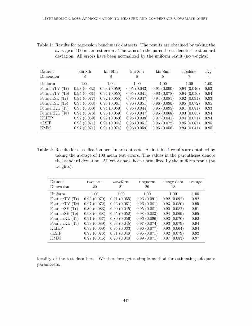
Table 1: Results for regression benchmark datasets. The results are obtained by taking theaverage of 100 mean test errors. The values in the parentheses denote the standarddeviation. All errors have been normalized by the uniform result (no weights).

Dataset kin-8fh kin-8fm kin-8nh kin-8nm abalone avgDimension 8 8 8 8 7 -

Uniform 1.00 1.00 1.00 1.00 1.00 1.00Fourier:TV (Tr) 0.93 (0.062) 0.93 (0.059) 0.95 (0.043) 0.91 (0.090) 0.94 (0.046) 0.93Fourier:TV (Te) 0.95 (0.061) 0.94 (0.055) 0.95 (0.041) 0.93 (0.078) 0.94 (0.056) 0.94Fourier:SE (Tr) 0.94 (0.077) 0.92 (0.055) 0.95 (0.047) 0.94 (0.081) 0.92 (0.091) 0.93Fourier:SE (Te) 0.95 (0.063) 0.93 (0.061) 0.96 (0.051) 0.96 (0.090) 0.95 (0.072) 0.95Fourier:KL (Tr) 0.93 (0.060) 0.94 (0.050) 0.95 (0.044) 0.95 (0.095) 0.91 (0.081) 0.93Fourier:KL (Te) 0.94 (0.078) 0.96 (0.059) 0.95 (0.047) 0.95 (0.068) 0.93 (0.085) 0.94KLIEP 0.92 (0.069) 0.92 (0.063) 0.95 (0.038) 0.97 (0.041) 0.94 (0.071) 0.94uLSIF 0.98 (0.071) 0.94 (0.044) 0.96 (0.051) 0.96 (0.072) 0.95 (0.067) 0.95KMM 0.97 (0.071) 0.94 (0.074) 0.96 (0.059) 0.95 (0.056) 0.93 (0.041) 0.95

Table 2: Results for classification benchmark datasets. As in table 1 results are obtained bytaking the average of 100 mean test errors. The values in the parentheses denotethe standard deviation. All errors have been normalized by the uniform result (noweights).

Dataset twonorm waveform ringnorm image data averageDimension 20 21 20 18 -

Uniform 1.00 1.00 1.00 1.00 1.00Fourier:TV (Tr) 0.92 (0.079) 0.91 (0.055) 0.96 (0.091) 0.92 (0.092) 0.92Fourier:TV (Te) 0.97 (0.072) 0.96 (0.061) 0.96 (0.081) 0.93 (0.080) 0.95Fourier:SE (Tr) 0.89 (0.083) 0.90 (0.045) 0.95 (0.081) 0.90 (0.082) 0.91Fourier:SE (Te) 0.93 (0.068) 0.95 (0.052) 0.98 (0.083) 0.94 (0.069) 0.95Fourier:KL (Tr) 0.91 (0.067) 0.89 (0.056) 0.96 (0.096) 0.93 (0.076) 0.92Fourier:KL (Te) 0.93 (0.089) 0.93 (0.045) 0.97 (0.074) 0.93 (0.079) 0.94KLIEP 0.93 (0.069) 0.95 (0.033) 0.96 (0.077) 0.93 (0.064) 0.94uLSIF 0.93 (0.076) 0.91 (0.048) 0.95 (0.071) 0.92 (0.079) 0.92KMM 0.97 (0.045) 0.98 (0.040) 0.99 (0.071) 0.97 (0.083) 0.97

locality of the test data here. We therefore get a simple method for estimating adequateparameters.

447

Vanck Garcke

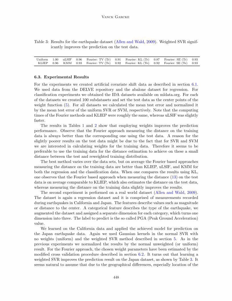
Table 3: Results for the earthquake dataset (Allen and Wald, 2009). Weighted SVR signif-icantly improves the prediction on the test data.

Uniform 1.00 uLSIF 0.96 Fourier: TV (Tr) 0.91 Fourier: KL (Tr) 0.87 Fourier: SE (Tr) 0.93KLIEP 0.96 KMM 0.93 Fourier: TV (Te) 0.92 Fourier: KL (Te) 0.92 Fourier: SE (Te) 0.93

6.3. Experimental Results

For the experiments we created artificial covariate shift data as described in section 6.1.We used data from the DELVE repository and the abalone dataset for regression. Forclassification experiments we obtained the IDA datasets available on mldata.org. For eachof the datasets we created 100 subdatasets and set the test data as the center points of theweight function (5). For all datasets we calculated the mean test error and normalized itby the mean test error of the uniform SVR or SVM, respectively. Note that the computingtimes of the Fourier methods and KLIEP were roughly the same, whereas uLSIF was slightlyfaster.

The results in Tables 1 and 2 show that employing weights improves the predictionperformance. Observe that the Fourier approach measuring the distance on the trainingdata is always better than the corresponding one using the test data. A reason for theslightly poorer results on the test data might be due to the fact that for SVR and SVMwe are interested in calculating weights for the training data. Therefore it seems to bepreferable to use the training data for the distance estimation to achieve on these a smalldistance between the test and reweighted training distribution.

The best method varies over the data sets, but on average the Fourier based approachesmeasuring the distance on the training data are better than KLIEP, uLSIF, and KMM forboth the regression and the classification data. When one compares the results using KL,one observes that the Fourier based approach when measuring the distance (13) on the testdata is on average comparable to KLIEP, which also estimates the distance on the test data,whereas measuring the distance on the training data slightly improves the results.

The second experiment is performed on a real world dataset (Allen and Wald, 2009).The dataset is again a regression dataset and it is comprised of measurements recordedduring earthquakes in California and Japan. The features describe values such as magnitudeor distance to the center. A categorical feature describes the type of the earthquake, weaugmented the dataset and assigned a separate dimension for each category, which turns onedimension into three. The label to predict is the so called PGA (Peak Ground Acceleration)value.

We learned on the California data and applied the achieved model for prediction onthe Japan earthquake data. Again we used Gaussian kernels in the normal SVR withno weights (uniform) and the weighted SVR method described in section 5. As in theprevious experiments we normalized the results by the normal unweighted (or uniform)result. For the Fourier approach, the chosen weight parameters have been estimated by themodified cross validation procedure described in section 6.2. It turns out that learning aweighted SVR improves the prediction result on the Japan dataset, as shown by Table 3. Itseems natural to assume that due to the geographical differences, especially location of the

448


measurements, there occurs a natural shift in the data, but that the implications remainthe same for the PGA value. Our experiments show that the application of weights to theregression method considerably improves the results, where the Fourier based approachesshow even more error reduction than the uLSIF, KMM, and KLIEP methods.

7. Conclusion

In this work we introduced a new method for measuring and compensating the covariateshift. We derived a new formulation for finding appropriate importance weights by usinga Fourier approximation of the divergence measure between the test distribution and thereweighted training distribution which does not make explicit use of the density functionsand takes a more function centric view than other data centered approaches. Higher dimen-sional problems can be treated by using a hyperbolic cross approximation in Fourier space.An advantage is that it enables the calculation of less volatile and therefore better weightsespecially in cases of small bandwidth parameters σ. Furthermore, the new approach givesa flexible framework since it can handle different divergence measures and can use any pointset for the empirical estimation of the divergence. Besides investigating further divergencemeasures we in particular are interested in the influence of the choice of the points wherethe divergence is measured, besides training and test points one here could also think aboutusing Smolyak quadrature points (Smolyak, 1963) or Quasi-Monte-Carlo sequences (Dicket al., 2013).

Note that currently all attributes are treated equally, but the hyperbolic cross approachcan be extended to have different resolutions in each dimension, which corresponds todimension-dependent smoothness properties. In such a case a dimension-adaptive choice ofthe Fourier resolution in the different dimensions can be achieved in a similar fashion to thatdescribed in Gerstner and Griebel (2003). Such an approach would allow the treatment ofeven higher dimensional problems.

Finally, the approach for compensating covariate shift is not limited to the currentchoice of a linear combination of (Gaussian) kernels for the weight function. An interestingpossibility would be the use of a sparse grid-based approach (Garcke, 2006; Pfluger, 2010),where the same underlying idea of a sparse tensor product construction and Sobolev spaceswith dominating mixed smoothness as for the hyperbolic cross approximation exists.

References

T.I. Allen and D.J. Wald. Evaluation of ground-motion modeling techniques for use in globalshakemap—a critique of instrumental ground-motion prediction equations, peak groundmotion to macroseismic intensity conversions, and macroseismic intensity predictions indifferent tectonic settings. U.S. Geological Survey Open-File Report 2009—1047, 2009.

K.I. Babenko. Approximation by trigonometric polynomials in a certain class of periodicfunctions of several variables. Sov. Math., Dokl., 1:672–675, 1960.

S. Bickel, M. Bruckner, and T. Scheffer. Discriminative learning under covariate shift.Journal of Machine Learning Research, 10, 2009.

O. Chapelle, B. Scholkopf, and A. Zien. Semi-Supervised Learning. MIT Press, 2006.

449

Vanck Garcke

J. Dick, F. Kuo, and I. Sloan. High-dimensional integration: The quasi-Monte Carlo way.Acta Numerica, 22:133–288, April 2013. doi: 10.1017/S0962492913000044.

J. Garcke. Regression with the optimised combination technique. In W. Cohen andA. Moore, editors, Proceedings of the 23rd ICML ’06, pages 321–328, 2006.

T. Gerstner and M. Griebel. Dimension–Adaptive Tensor–Product Quadrature. Computing,71(1):65–87, 2003.

J. Huang, A. J. Smola, A. Gretton, K. M. Borgwardt, and B. Scholkopf. Correcting sampleselection bias by unlabeled data. In NIPS 19, pages 601–608, 2007.

T. Kanamori, S. Hido, and M. Sugiyama. A least-squares approach to direct importanceestimation. The Journal of Machine Learning, 10:1391–1445, 2009.

S. Knapek. Hyperbolic cross approximation of integral operators with smooth kernel. Tech-nical Report 665, SFB 256, Univ. Bonn, 2000. URL http://wissrech.ins.uni-bonn.

de/research/pub/knapek/fourier.ps.gz.

J. Moreno-Torres, T. Raeder, R. Alaiz-Rodrıguez, N. Chawla, and F. Herrera. A unifyingview on dataset shift in classification. Pattern Recognition, 45(1):521–530, January 2012.doi: 10.1016/j.patcog.2011.06.019.

D. Pfluger. Spatially Adaptive Sparse Grids for High-Dimensional Problems. Verlag Dr.Hut, 2010.

J. Quionero-Candela, M. Sugiyama, A. Schwaighofer, and N. Lawrence. Dataset Shift inMachine Learning. The MIT Press, 2009.

S. A. Smolyak. Quadrature and interpolation formulas for tensor products of certain classesof functions. Dokl. Akad. Nauk SSSR, 148:1042–1043, 1963. Russian, Engl.: Soviet Math.Dokl. 4:240–243, 1963.

M. Sugiyama and M. Kawanabe. Machine learning in non-stationary environments: Intro-duction to covariate shift adaptation. MIT Press, Cambridge, Mass., 2012.

M. Sugiyama, M. Krauledat, and K.-R. Muller. Covariate shift adaptation by importanceweighted cross validation. Journal of Machine Learning Research, 8:985–1005, 2007.

M. Sugiyama, S. Nakajima, H. Kashima, P. Bunau, and M. Kawanabe. Direct importanceestimation with model selection and its application to covariate shift adaptation. In NIPS20, pages 1433–1440, 2008.

Y. Tsuboi, H. Kashima, S. Hido, S. Bickel, and M. Sugiyama. Direct density ratio estimationfor large-scale covariate shift adaptation. Journal of Information Processing, 17:138–155,2009.

Din’ Zung. The approximation of classes of periodic functions of many variables. RussianMathematical Surveys, 38(6):117–118, December 1983.

450

http://wissrech.ins.uni-bonn.de/research/pub/knapek/fourier.ps.gz

http://wissrech.ins.uni-bonn.de/research/pub/knapek/fourier.ps.gz

Documents

Using Hyperbolic Cross Approximation to measure and compensate