Using Gaussian Process Annealing ParticleFilter for 3D Human Tracking

Leonid Raskin, Ehud Rivlin, Michael Rudzsky

Computer Science Department,Technion Israel Institute of Technology,Technion City, Haifa, Israel

raskinl, ehudr, rudzsky@cs.technion.ac.il

Abstract. We present an approach for human body parts tracking in3D with prelearned motion models using multiple cameras. GaussianProcess Annealing Particle Filter is proposed for tracking in order toreduce the dimensionality of the problem and to increase the tracker’sstability and robustness. Comparing with a regular annealed particlefilter based tracker, we show that our algorithm can track better forlow frame rate videos. We also show that our algorithm is capable ofrecovering after a temporal target loose.

1 Introduction

Human body pose estimation and tracking is a challenging task for several rea-sons. First, the large dimensionality of the human 3D model complicates theexamination of the entire subject and makes it harder to detect each body partseparately. Secondly, the significantly different appearance of different peoplethat stems from various clothing styles and illumination variations, adds to thealready great variety of images of different individuals. Finally, the most chal-lenging difficulty that has to be solved in order to achieve satisfactory results ofpose understanding is the ambiguity caused by body.

This paper presents an approach to 3D articulated human body tracking,that enables reduction of the complexity of this model. We propose a novelalgorithm, Gaussian Process Annealed Particle Filter (GPAPF) (see also Raskinet al. [11, 26]). In this algorithm we apply a nonlinear dimensionality reductionusing Gaussian Process Dynamical Model (GPDM) (Lawrence [7], Wang et al.[19]) in order to create a low dimensional latent space. This space describes posesfrom a specific motion type. Later we use annealed particle filter proposed byDeutscher and Reid [3, 15] that operates in this laten space in order to generateparticles.

The annealed particle filter has a good performance when applied on videoswith a high frame rate (60 fps, as reported by Balan et al. [5]), but performancedrops when the frame rate is lower (30fps). We show that our approach providesgood results even for the low frame rate (30 fps and lower). An additional ad-vantage of our tracking algorithm is the capability to recover after temporal lossof the target, which makes the tracker more robust.

2 Related Works

There are two main approaches for body pose estimation. The first one is thebody detection and recognition, which is based one a single frame (Perona etal. [33], Ioffe et al. [30], Mori et al. [12]). The second approach is the bodypose tracking which approximates body pose based on a sequence of frames(Sidenbladh et al. [27], Davidson et al. [14], Agarwal et al. [2, 1]). A variety ofmethods have been developed for tracking people from single views (Ramananet al. [9]), as well as from multiple views (Deutscher et al. [3]).

One of the common approaches for tracking is using particle filtering meth-ods. Particle Filtering uses multiple predictions, obtained by drawing samples ofpose and location prior and then propagating them using the dynamic model,which are refined by comparing them with the local image data, calculating thelikelihood (see, for example Isard and MacCormick [24] or Bregler and Malik[6]). The prior is typically quite diffused (because motion can be fast) but thelikelihood function may be very peaky, containing multiple local maxima whichare hard to account for in detail. For example, if an arm swings past an arm-like pole, the correct local maximum must be found to prevent the track fromdrifting (Sidenbladh et al. [17]). Annealed particle filter (Deutscher et al. [15])or local searches are the ways to attack this difficulty. An alternative is to applya strong model of dynamics (Mikolajcyk et al. [20]).

There exist several possible strategies for reducing the dimensionality of theconfiguration space. Firstly it is possible to restrict the range of movement of thesubject. This approach has been pursued by Rohr [21]. The assumption is thatthe subject is performing a specific action. Agarwal and Triggs [2, 1] assume aconstant angle of view of the subject. Because of the restricting assumptions theresulting trackers are not capable of tracking general human poses. Several workshave been done in attempt to learn subspace models. For example, Ormoneit etal. [25] has used PCA on the cyclic motions. Another way to cope with high-dimensional data space is to learn low-dimensional latent variable models [4, 13].However, methods like Isomap [10] and locally linear embedding (LLE) [31] donot provide a mapping between the latent space and the data space. Urtasun etal. [29, 28, 18] uses a form of probabilistic dimensionality reduction by GaussianProcess Dynamical Model (GPDM) (Lawrence [7], and Wang et al. [19]) andformulate the tracking as a nonlinear least-squares optimization problem.

We propose a tracking algorithm, which consists of two stages. We separatethe body model state into two independent parts: the first one contains informa-tion about 3D location and orientation of the body and the second one describesthe pose. We learn latent space that describes poses only. In the first one wegenerate particles in the latent space and transform them into the data spaceby using learned a priori mapping function. In the second stage we add rotationand translation parameters to obtain valid poses. Then we project the poses onthe cameras in order to calculate the weighted function.

The article is organized as follows. In Section 3 and Section 4 we give adescription of particle filtering and Gaussian fields. In Section 5, we describeour algorithm. Section 6 contains our experimental results and comparison to

annealed particle filter tracker. The conclusions and possible extension are givenin Section 7.

3 Filtering

3.1 Particle filter

The particle filter algorithm was developed for tracking objects, using the Bayesianinference framework. In order to make an estimation of the tracked object pa-rameter this algorithm suggests using the importance sampling. Importance sam-pling is a general technique for estimating the statistics of a random variable.The estimation is based on samples of this random variable generated from otherdistribution, called proposal distribution, which is easy to sample from.

Let us denote xn as a hidden state vector and yn be a measurement in timen. The algorithm builds an approximation of a maximum posterior estimate ofthe filtering distribution: p (xn|y1:n), where y1:n ≡ (y1, ..., yn) is the history of

the observation. This distribution is represented by a set of pairs

x(i)n ; π(i)

n

Np

i=1,

where π(i)n ∝ p

(yn|x(i)

n

). Using Bayes’ rule, the filtering distribution can be

calculated using two steps: Prediction step:

p (xn|y1:n−1) =∫

p (xn|xn−1) p (xn−1|y1:n−1) dxn−1 (1)

Filtering step:p (xn|y1:n) ∝ p (yn|xn) p (xn|y1:n−1) (2)

Therefore, starting with a weighted set of samples

x(i)0 ;π(i)

0

Np

i=1, the new

sample set

x(i)n ; π(i)

n

Np

i=1is generated according to the distribution, that may

depend on the previous set

x(i)n−1;π

(i)n−1

Np

i=1and the new measurements yn:

x(i)n ∼ q

(x

(i)n |x(i)

n−1, yn

), i = 1, ..., Np. The new weights are calculated using the

following formula:

π(i)n = kπ(i)

n

p(yn|x(i)

n

)p

(x

(i)n |x(i)

n−1

)

q(x

(i)n |x(i)

n−1, yn

) (3)

where

k =

Np∑

i=1

π(i)n

p(yn|x(i)

n

)p

(x

(i)n |x(i)

n−1

)

q(x

(i)n |x(i)

n−1, yn

)−1

(4)

and q(x

(i)n |x(i)

n−1, yn

)is the proposal distribution.

The main problem is that the distribution p (yn|xn) may be very peaky andfar from being convex. For such p (yn|xn) the algorithm usually detects severallocal maxima instead of choosing the global one (see Deutscher and Reid [15]).This usually happens for the high dimensional problems, like body part track-ing. In this case a large number of samples have to be taken in order to findthe global maxima, instead of choosing a local one. The other problem thatarises is that the approximation of the p (xn|y1:n) for high dimensional spacesis a very computationally inefficient and hard task. Often a weighting functionwi

n (yn, x) can be constructed according to the likelihood function as it is in thecondensation algorithm of Isard and Blake [23], such that it provides a goodapproximation of the p (yn|xn) , but is also relatively easy to calculate. There-fore, the problem becomes to find configuration xk that maximizes the weightingfunction wi

n (yn, x).

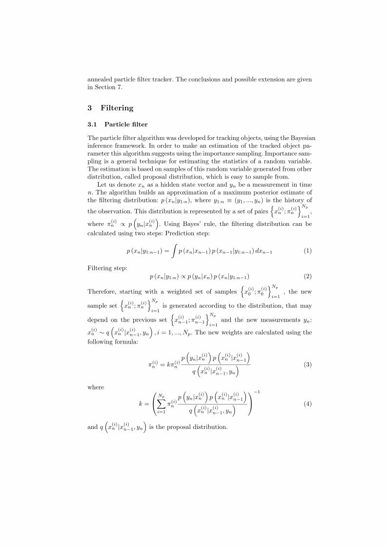
3.2 Annealed Particle Filter

The main idea is to use a set of weighting functions instead of using a single one.While a single weighting function may contain several local maxima, the weight-ing function in the set should be smoothed versions of it, and therefore contain asingle maximum point, which can be detected using the regular annealed particlefilter.

Fig. 1. Annealed particle filter illustration for M=5 . Initially the set contains manyparticles that represent very different poses and therefore can fall into local maximum.On the last layer all the particles are close to the global maximum, and therefore theyrepresent the correct pose.

A series of wm (yn, x)Mm=0 is used, where wm−1 (yn, x) differs only slightly

from wm (yn, x) and represents a smoothed version of it. The samples shouldbe drawn from the w0 (yn, x) function, which might be peaky, and therefore alarge number of particles needed to be used in order to find the global maxima.Therefore, wM (yn, x) is designed to be a very smoothed version of w0 (yn, x) .The usual method to achieve this is by using wm (yn, x) = (w0 (yn, x))βm , where1 = β0 > ... > βM and w0 (yn, x) is equal to the original weighting function.Therefore, each iteration of the annealed particle filter algorithm consists of Msteps, in each of these the appropriate weighting function is used and a set of

pairs is constructed

x(i)n,m; π(i)

n,m

Np

i=1. Tracking is described in Algorithm 1.

Fig. 1 shows the illustration of the 5-layered annealing particle filter. Initiallythe set contain many particles that represent very different poses and thereforecan fall into local maximum. On the last layer all the particles are close to theglobal maximum, and therefore they represent the correct pose.

Algorithm 1 : The annealed particle filter algorithm

Initialization:

x(i)n,M ; 1

N

Np

i=1for each: frame n

for m = M downto 0 do

1. Calculate the weights: π(i)n = k

wm(

yn,x(i)n,m

)p(

x(i)n,m|x(i)

n,m−1

)

q(

x(i)n,m|x(i)

n,m−1,yn

) , where

k =

(∑Np

i=1

wm(

yn|x(i)n,m

)p(

x(i)n,m|x(i)

n,m−1

)

q(

x(i)n,m|x(i)

n,m−1,yn

))−1

.

2. Draw N particles from the weighted set

x(i)n,m; π

(i)n,m

Np

i=1with replacement and

with distribution p(x = x

(i)n,m

)= π

(i)n,m.

3. Calculate x(i)n,m−1 ∼ q

(x

(i)n,m−1|x(i)

n,m, yn

)= x

(i)n,m +nm, where nm is a Gaussian

noise nm N (0, Pm).end for- The optimal configuration can be calculated using the following formula: xn =∑Np

i=1 π(i)n,0x

(i)n,0.

- The unweighted particle set for the next observation is produced using x(i)n+1,M =

x(i)n,0 + n0, where n0 is a Gaussian noise nm N (0, P0).

end for each

4 Gaussian Fields

The Gaussian Process Dynamical Model (GPDM) (Lawrence [7], Wang et al.[19]) represents a mapping from the latent space to the data: y = f (x), wherex ∈ IRd denotes a vector in a d -dimensional latent space and y ∈ IRD is avector, that represents the corresponding data in a D-dimensional space. The

model that is used to derive the GPDM is a mapping with first-order Markovdynamics:

xt =∑

i

aiφi (xt−1) + nx,t

yt =∑

j

bjψj (xt) + ny,t

(5)

where nx,t and ny,t are zero-mean Gaussian noise processes, A = [a1, a2, ...] andB = [b1, b2, ...] are weights and φj and ψj are basis functions.

For Bayesian perspective A and B should be marginalized out through modelaverage with an isotropic Gaussian prior on B in closed form to yield:

P(Y |X, β

)=

|W |N√(2π)ND|Ky|D

e−12 tr(K−1

y Y W 2Y T ) (6)

where W is a scaling diagonal matrix, Y is a matrix of training vectors, Xcontains corresponding latent vectors and Ky is the kernel matrix:

(Ky)i,j = β1e− β2

2 ‖xi−xj‖ +δxi,xj

β3(7)

W is a scaling diagonal matrix. It is used to account for the different variancesin different data elements. The hyper parameter β1 represents the scale of theoutput function, β2 represents the inverse of the Radial Basis Function (RBF)and β−1

3 represents the variance of ny,t . For the dynamic mapping of the latentcoordinates X the joint probability density over the latent coordinate systemand the dynamics weights A are formed with an isotropic Gaussian prior overthe A, it can be shown (see Wang et al. [19]) that

P (X|α) =P (x1)√

(2π)(N−1)d|Kx|de−

12 tr(K−1

x XoutXTout) (8)

where Xout = [x2, ..., xN ]T , Kx is a kernel constructed from [x1, ..., xN−1]T and

x1 has an isotropic Gaussian prior. GPDM uses a ”linear+RBF” kernel withparameter αi :

(Ky)i,j = α1e−α2

2 ‖xi−xj‖ + α3xTi xj +

δxi,xj

α4(9)

Following Wang et al. [19]

P(X, α, β|Y ) ∝ P

(Y |X, β

)P (X|α)P (α)P

(β)

(10)

the latent positions and hyper parameters are found by maximizing this distri-bution or minimizing the negative log posterior:

Λ =d

2ln|Kx|+ 1

2tr

(K−1

x XoutXTout

)+

∑

i

lnαi −Nln|W |+

+D

2ln|Ky|+ 1

2tr

(K−1

y Y W 2XT)

+∑

i

lnβi (11)

5 GPAPF Filtering

5.1 The Model

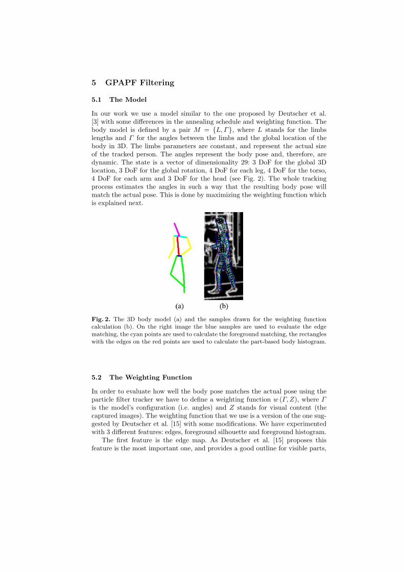
In our work we use a model similar to the one proposed by Deutscher et al.[3] with some differences in the annealing schedule and weighting function. Thebody model is defined by a pair M = L, Γ, where L stands for the limbslengths and Γ for the angles between the limbs and the global location of thebody in 3D. The limbs parameters are constant, and represent the actual sizeof the tracked person. The angles represent the body pose and, therefore, aredynamic. The state is a vector of dimensionality 29: 3 DoF for the global 3Dlocation, 3 DoF for the global rotation, 4 DoF for each leg, 4 DoF for the torso,4 DoF for each arm and 3 DoF for the head (see Fig. 2). The whole trackingprocess estimates the angles in such a way that the resulting body pose willmatch the actual pose. This is done by maximizing the weighting function whichis explained next.

Fig. 2. The 3D body model (a) and the samples drawn for the weighting functioncalculation (b). On the right image the blue samples are used to evaluate the edgematching, the cyan points are used to calculate the foreground matching, the rectangleswith the edges on the red points are used to calculate the part-based body histogram.

5.2 The Weighting Function

In order to evaluate how well the body pose matches the actual pose using theparticle filter tracker we have to define a weighting function w (Γ,Z), where Γis the model’s configuration (i.e. angles) and Z stands for visual content (thecaptured images). The weighting function that we use is a version of the one sug-gested by Deutscher et al. [15] with some modifications. We have experimentedwith 3 different features: edges, foreground silhouette and foreground histogram.

The first feature is the edge map. As Deutscher et al. [15] proposes thisfeature is the most important one, and provides a good outline for visible parts,

such as arms and legs. The other important property of this feature is that itis invariant to the color and lighting condition. The edge maps, in which eachpixel is assigned a value dependent on its proximity to an edge, are calculatedfor each image plane. Each part is projected on the image plane and samplesof the Ne hypothesized edges of human body model are drawn. A sum-squareddifference function is calculated for these samples:

Σe (Γ, Z) =1

Ncv

1Ne

Ncv∑

i=1

Ne∑

j=1

(1− pe

j (Γ,Zi))2 (12)

where Ncv is a number of camera views, and Zi stands for the image from thei -th camera . The pe

j (Γ, Zi) are the edge maps. Each part is projected on theimage plane and samples of the Ne hypothesized edges are drawn.

However, the problem that occurs using this feature is that the occludedbody parts will produce no edges. Even the visible parts, such as the arms, maynot produce the edges, because of the color similarity between the part andthe body. This will cause pe

j (Γ,Zi) to be close to zero and thus will increasethe squared difference function. Therefore, a good pose which represents wellthe visual context may be omitted. In order to overcome this problem for eachcombination of image plane and body part we calculate a coefficient, whichindicates how well the part can be observed on this image. For each samplepoint on the model’s edge we estimate the probability being covered by anotherbody part. Let Ni be the number of hypothesized edges that are drawn forthe part i. The total number of drawn sample points can be calculated usingNe =

∑Nbp

i=1 Ni, where Nbp is the total number of body parts in the model. Thecoefficient of part i for the image plane j can be calculated as following:

λi,j =1Ni

Ni∑

k=1

(1− pfg

k (Γi, Zj))2

(13)

where Γi is the model configuration for part i and pfgk (Γi, Zj) is the value of the

foreground pixel map of the sample k. If a body part is occluded by another one,then the value of pfg

k (Γi, Zj) will be close to one and therefore the coefficientof this part for the specific camera will be low. We propose using the followingfunction instead of sum-squared difference function as presented in (12):

Σe (Γ,Z) =1

Ncv

1Ne

Nbp∑

i=1

Ncv∑

j=1

λi,jΣ (Γi, Zj) (14)

where

Σ (Γbp, Zcv) =Ni∑

k=1

(1− pek (Γbp, Zcv))2 (15)

The second feature is the silhouette obtained by subtracting the backgroundfrom the image. The foreground pixel map is calculated for each image plane with

background pixels set to 0 and foreground set to 1 and sum squared differencefunction is computed:

Σfg (Γ, Z) =1

Ncv

1Ne

Ncv∑

i=1

Ne∑

j=1

(1− pfg

j (Γ,Zi))2

(16)

where pfgj (Γ, Zi) is the value is the foreground pixel map values at the sample

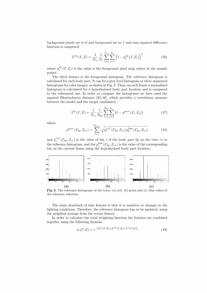
points.The third feature is the foreground histogram. The reference histogram is

calculated for each body part. It can be a grey level histogram or three separatedhistograms for color images, as shown in Fig. 3. Then, on each frame a normalizedhistogram is calculated for a hypothesized body part location and is comparedto the referenced one. In order to compare the histograms we have used thesquared Bhattacharya distance [32, 16], which provides a correlation measurebetween the model and the target candidates :

Σh (Γ, Z) =1

Ncv

1Nbp

Nbp∑

i=1

Ncv∑

j=1

(1− ρpart (Γi, Zj)

)(17)

where

ρpart (Γbp, Zcv) =Nbins∑

i=1

√pref

i (Γbp, Zcv) phypk (Γbp, Zcv) (18)

and prefi (Γbp, Zcv) is the value of bin i of the body part bp on the view cv in

the reference histogram, and the phypi (Γbp, Zcv) is the value of the corresponding

bin on the current frame using the hypothesized body part location.

Fig. 3. The reference histograms of the torso: (a) red, (b) green and (c) blue colors ofthe reference selection.

The main drawback of that feature is that it is sensitive to changes in thelighting conditions. Therefore, the reference histogram has to be updated, usingthe weighted average from the recent history.

In order to calculate the total weighting function the features are combinedtogether using the following formula:

w (Γ, Z) = e−(Σe(Γ,Z)+Σfg(Γ,Z)+Σh(Γ,Z)) (19)

As was stated above, the target of the tracking process is equal to maximizingthe weighting function.

5.3 GPAPF Learning

The drawback in the particle filter tracker is that a high dimensionality of thestate space causes an exponential increase in the number of particles that areneeded to be generated in order to preserve the same density of particles. Inour case, the data dimension is 29-D. In their work Balan et al. [5] show thatthe annealed particle filter is capable of tracking body parts with 125 particlesusing 60 fps video input. However, using a significantly lower frame rate (15 fps)causes the tracker to produce bad results and eventually to lose the target.

The other problem of the annealed particle filter tracker is that once a targetis lost (i.e. the body pose was wrongly estimated, which can happen for the fastand not smooth movements) it is highly unlikely that the pose on the followingframes will be estimated correctly.

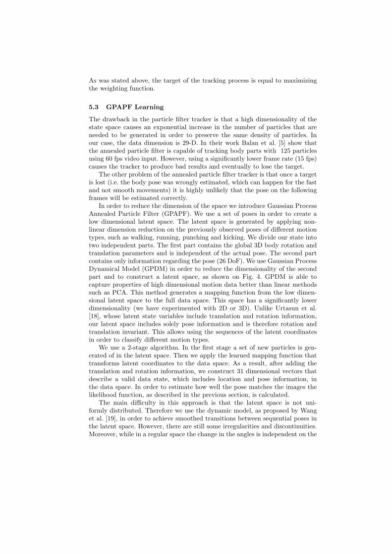
In order to reduce the dimension of the space we introduce Gaussian ProcessAnnealed Particle Filter (GPAPF). We use a set of poses in order to create alow dimensional latent space. The latent space is generated by applying non-linear dimension reduction on the previously observed poses of different motiontypes, such as walking, running, punching and kicking. We divide our state intotwo independent parts. The first part contains the global 3D body rotation andtranslation parameters and is independent of the actual pose. The second partcontains only information regarding the pose (26 DoF). We use Gaussian ProcessDynamical Model (GPDM) in order to reduce the dimensionality of the secondpart and to construct a latent space, as shown on Fig. 4. GPDM is able tocapture properties of high dimensional motion data better than linear methodssuch as PCA. This method generates a mapping function from the low dimen-sional latent space to the full data space. This space has a significantly lowerdimensionality (we have experimented with 2D or 3D). Unlike Urtasun et al.[18], whose latent state variables include translation and rotation information,our latent space includes solely pose information and is therefore rotation andtranslation invariant. This allows using the sequences of the latent coordinatesin order to classify different motion types.

We use a 2-stage algorithm. In the first stage a set of new particles is gen-erated of in the latent space. Then we apply the learned mapping function thattransforms latent coordinates to the data space. As a result, after adding thetranslation and rotation information, we construct 31 dimensional vectors thatdescribe a valid data state, which includes location and pose information, inthe data space. In order to estimate how well the pose matches the images thelikelihood function, as described in the previous section, is calculated.

The main difficulty in this approach is that the latent space is not uni-formly distributed. Therefore we use the dynamic model, as proposed by Wanget al. [19], in order to achieve smoothed transitions between sequential poses inthe latent space. However, there are still some irregularities and discontinuities.Moreover, while in a regular space the change in the angles is independent on the

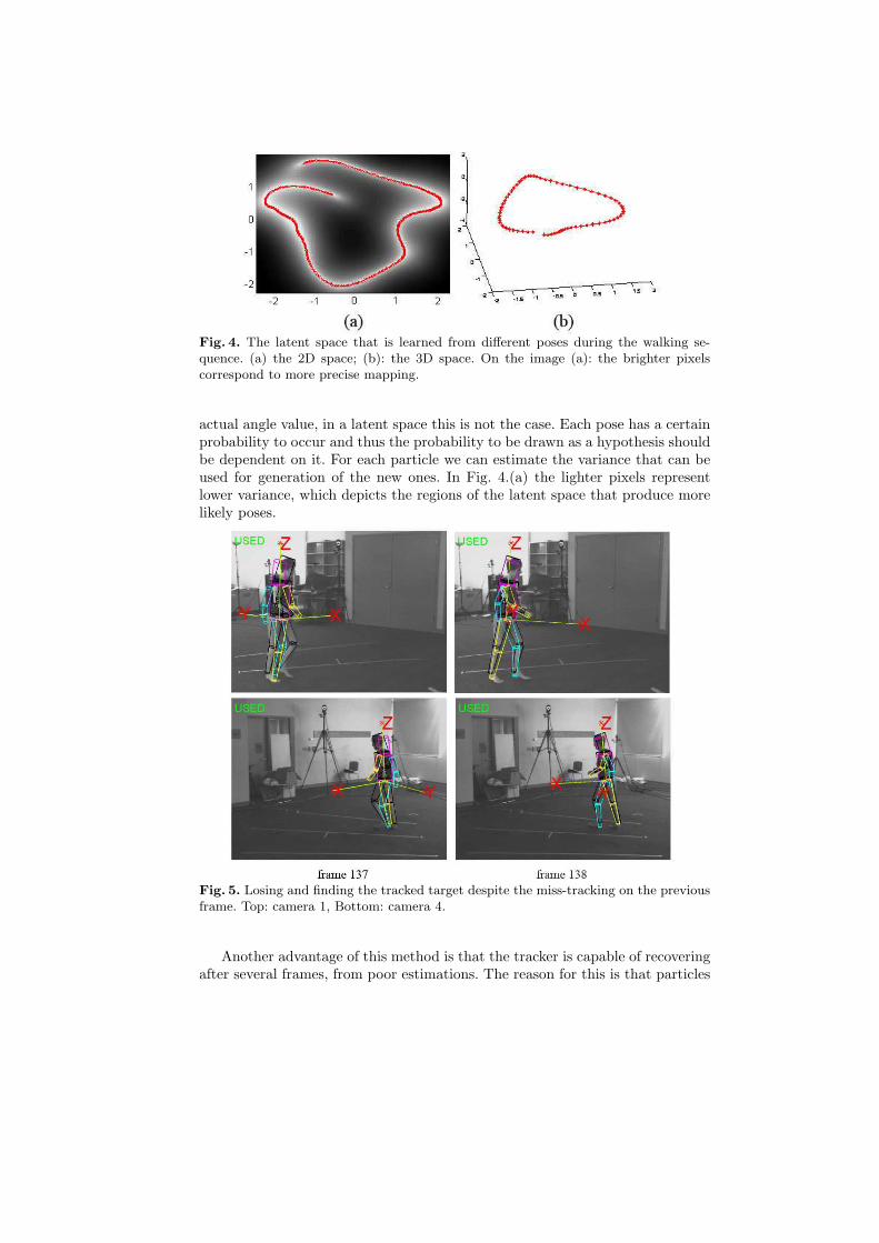
Fig. 4. The latent space that is learned from different poses during the walking se-quence. (a) the 2D space; (b): the 3D space. On the image (a): the brighter pixelscorrespond to more precise mapping.

actual angle value, in a latent space this is not the case. Each pose has a certainprobability to occur and thus the probability to be drawn as a hypothesis shouldbe dependent on it. For each particle we can estimate the variance that can beused for generation of the new ones. In Fig. 4.(a) the lighter pixels representlower variance, which depicts the regions of the latent space that produce morelikely poses.

Fig. 5. Losing and finding the tracked target despite the miss-tracking on the previousframe. Top: camera 1, Bottom: camera 4.

Another advantage of this method is that the tracker is capable of recoveringafter several frames, from poor estimations. The reason for this is that particles

generated in the latent space are representing valid poses more authentically.Furthermore because of its low dimensionality the latent space can be coveredwith a relatively small number of particles. Therefore, most of possible poses willbe tested with emphasis on the pose that is close to the one that was retrievedin the previous frame. So if the pose was estimated correctly the tracker will beable to choose the most suitable one from the tested poses. However, if the poseon the previous frame was miscalculated the tracker will still consider the posesthat are quite different. As these poses are expected to get higher value of theweighting function the next layers of the annealing process will generate manyparticles using these different poses. As shown in Fig. 5 in this way the pose islikely to be estimated correctly, despite the miss-tracking on the previous frame.

In addition the generated poses are, in most cases, natural. The large vari-ance in the data space causes the generation of unnatural poses by the CON-DENSATION or by annealed particle filtering algorithms. In the introducedapproach the poses that are produced by the latent space that correspond topoints with low variance are usually natural as the whole latent space is con-structed based on learning from a set of valid poses. The unnatural posescorrespond to the points with the large variance (black re-gions on Fig. 4.(a)) and, therefore, it is highly unlikely thatit will be generated. Therefore the effective number of the particles ishigher, which enables more accurate tracking.

As shown in Fig. 4 is that the latent space is not continuous. Two sequentialposes may appear not too close in the latent space; therefore there is a minimalnumber of particles that should be drawn in order to be able to perform thetracking.

The other drawback of this approach is that it requires more calculation thanthe regular annealed particle filter due to the transformation from the latentspace into the data space. However, as it is mentioned above, if same number ofparticles is used, the amount of the effective poses is significantly higher in theGPAPF then in the original annealed particle filter. Therefore, we can reducethe number of the particles for the GPAPF tracker, and by this compensate forthe additional calculations.

5.4 GPAPF Algorithm

As we have explained before we are using a 2-stage algorithm. The state consistsof 2 statistically independent parts. The first one describes the body 3D location:the rotation and the translation (6 DoF). The second part describes the actualpose i.e. the latent coordinates of the corresponding point in the Gaussian Space(that was generated as we have explained in part 5.3). The second part usuallyhas a very small DoF (as was mentioned before we have experimented with 2 and3 dimensional latent spaces). The first stage is the generation of new particles.Then we apply the learned transform function that transforms latent coordinatesto the data space (25 DoF). As the result, after adding the translation androtation information, we construct a 31 dimensional vectors that describe a validdata state, which includes location and pose information, in the data space. Then

the state is projected to the cameras in order to estimate how well it fits theimages.

Suppose we have M annealing layers. The state is defined as a pair Γ =Λ,Ω, where Λ is the location information and Ω is the pose information.We also define ω as a latent coordinates corresponding to the data vector Ω:Ω = ℘ (ω), where ℘ is the mapping function learned by the GPDM. Λn,m, Ωn,m

and ωn,m are the location, pose vector and corresponding latent coordinates onthe frame n and annealing layer m. For each 1 ≤ m ≤ M − 1 Λn,m and ωn,m

are generated by adding multi-dimensional Gaussian random variable to Λn,m+1

and ωn,m+1 respectively. Then Ωn,m is calculated using ωn,m. Full body stateΓn,m = Λn,m, Ωn,m is projected to the cameras and the likelihood πn,m iscalculated using likelihood function as explained in section 5.2 (see Algorithm2).

In the original annealed particle filter algorithm the optimal configuration isachieved by calculating the weighted average of the particles in the last layer.However, as the latent space is not an Euclidian one, applying this method onω will produce poor results. The other method is choosing the particle withthe highest likelihood as the optimal configuration ωn = ω

(imax)n,0 , where imax =

arg mini

(π

(i)n,m

). However, this is unstable way to calculate the optimal pose, as

in order to ensure that there exists a particle which represents the correct posewe have to use a large number of particles. Therefore, we propose to calculatethe optimal configuration in the data space and then project it back to the latentspace. At the first stage we apply the ℘ on all the particles to generate vectorsin the data space. Then in the data space we calculate the average on thesevectors and project it back to the latent space. It can be written as follows:ωn = ℘−1

(∑Ni=1 π

(i)n,0℘

(ω

(i)n,0

)).

5.5 Towards more precise tracking

The problem with such a 2-stage approach is that Gaussian field is not capa-ble to describe all possible posses. As we have mentioned above, this approachresembles using probabilistic PCA in order to reduce the data dimensionality.However, for tracking issues we are interested to get the pose estimation as closeas possible to the actual one. Therefore, we add an additional annealing layer asthe last step. This stage consists from only one stage. We use data states, whichwere generated on the previous 2 staged annealing layer, described in previoussection, in order to generate data states for the next layer. This is done withvery low variances in all the dimensions, which practically are equal for all ac-tions, as the purpose of this layer is to make only the slight changes in the finalestimated pose. Thus it does not depend on the actual frame rate, contrary tooriginal annealing particle tracker, where if the frame rate is changed one needto update the model parameters (the variances for each layer).

The final scheme of each step is shown in the Fig. 6 and described in Al-gorithm 3 . Suppose we have M annealing layers, as explained in section 5.4.

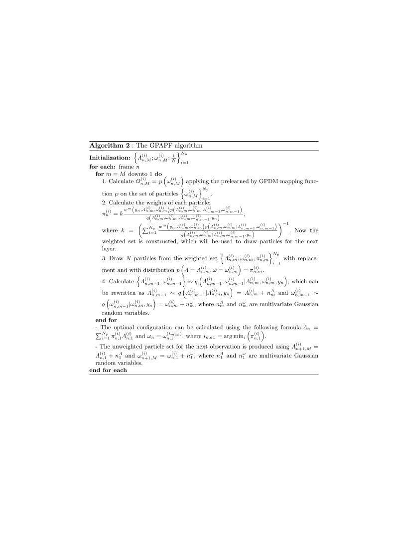
Algorithm 2 : The GPAPF algorithm

Initialization:

Λ(i)n,M ; ω

(i)n,M ; 1

N

Np

i=1for each: frame n

for m = M downto 1 do1. Calculate Ω

(i)n,M = ℘

(ω

(i)n,M

)applying the prelearned by GPDM mapping func-

tion ℘ on the set of particles

ω(i)n,M

Np

i=1.

2. Calculate the weights of each particle:

π(i)n = k

wm(

yn,Λ(i)n,m,ω

(i)n,m

)p(

Λ(i)n,m,ω

(i)n,m|Λ(i)

n,m−1,ω(i)n,m−1

)

q(

Λ(i)n,m,ω

(i)n,m|Λ(i)

n,m,ω(i)n,m−1,yn

) ,

where k =

(∑Np

i=1

wm(

yn,Λ(i)n,m,ω

(i)n,m

)p(

Λ(i)n,m,ω

(i)n,m|Λ(i)

n,m−1,ω(i)n,m−1

)

q(

Λ(i)n,m,ω

(i)n,m|Λ(i)

n,m,ω(i)n,m−1,yn

))−1

. Now the

weighted set is constructed, which will be used to draw particles for the nextlayer.

3. Draw N particles from the weighted set

Λ(i)n,m; ω

(i)n,m; π

(i)n,m

Np

i=1with replace-

ment and with distribution p(Λ = Λ

(i)n,m, ω = ω

(i)n,m

)= π

(i)n,m.

4. Calculate

Λ(i)n,m−1; ω

(i)n,m−1

∼ q

(Λ

(i)n,m−1; ω

(i)n,m−1|Λ(i)

n,m; ω(i)n,m, yn

), which can

be rewritten as Λ(i)n,m−1 ∼ q

(Λ

(i)n,m−1|Λ(i)

n,m, yn

)= Λ

(i)n,m + nΛ

m and ω(i)n,m−1 ∼

q(ω

(i)n,m−1|ω(i)

n,m, yn

)= ω

(i)n,m + nω

m, where nΛm and nω

m are multivariate Gaussian

random variables.end for- The optimal configuration can be calculated using the following formula:Λn =∑Np

i=1 π(i)n,1Λ

(i)n,1 and ωn = ω

(imax)n,1 , where imax = arg mini

(π

(i)n,1

).

- The unweighted particle set for the next observation is produced using Λ(i)n+1,M =

Λ(i)n,1 + nΛ

1 and ω(i)n+1,M = ω

(i)n,1 + nω

1 , where nΛ1 and nω

1 are multivariate Gaussianrandom variables.

end for each

Then we add one more single-staged layer. In this last layer the Ωn,0 is cal-culated using only the Ωn,1 without calculating the ωn,0. We should also payattention that the last layer has no influence of the quality of tracking in thefollowing frames, as ωn,1 is used for the initialization of the next layer. Fig. 7shows the difference between the version without the additional annealing layerand the results after adding it. We have used 5 2-staged annealing layers in bothcases. For the second tracker we have added additional single staged layer. Inthe Fig. 8 shows the error graph that were produced by two trackers. The errorwas calculated, based on comparison of the tracker’s output and the result ofthe MoCap system. The comparison was suggested by A. Balan [5]. This is doneby calculating the 3D distance between the locations of the different joints thatis estimated by the MoCap system and by the trackers results. The joints thatare used are hips, knees, etc. The distances are summed and multiplied by theweight of the corresponding particle. Then the sum of the all weighted distancesis calculated, which is used as an error measurement. We can see that the er-ror, produced by GPAPF tracker without the additional layer (blue circles onthe graph) is lower then the one produced by the original GPAPF algorithmwith the additional annealing layer (red crosses on the graph) for the walkingsequence taken at 30 fps. We can notice that the error is lower when we add thelayer. However, as we have expected, the improvement is not dramatic. This isexplained by the fact that the difference between the estimated pose using onlythe latent space annealing and the actual pose is not very big. That suggeststhat the latent space accurately represents the data space.

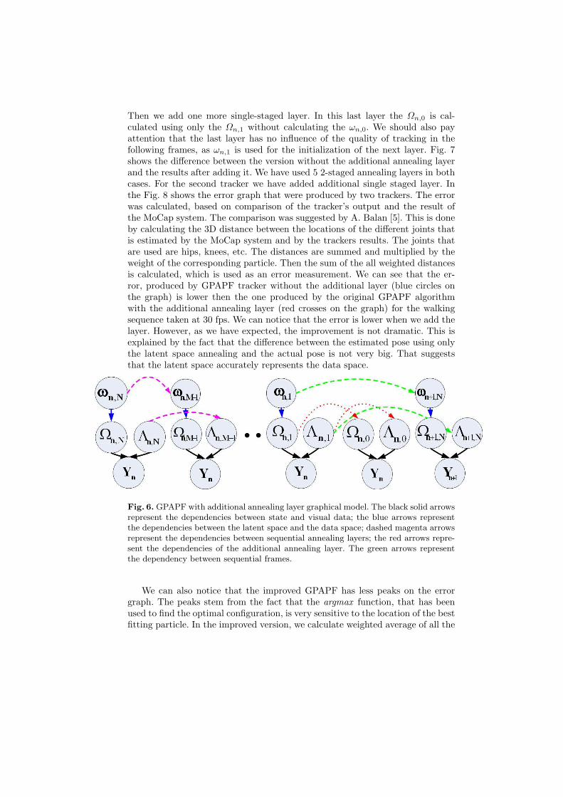
Fig. 6. GPAPF with additional annealing layer graphical model. The black solid arrowsrepresent the dependencies between state and visual data; the blue arrows representthe dependencies between the latent space and the data space; dashed magenta arrowsrepresent the dependencies between sequential annealing layers; the red arrows repre-sent the dependencies of the additional annealing layer. The green arrows representthe dependency between sequential frames.

We can also notice that the improved GPAPF has less peaks on the errorgraph. The peaks stem from the fact that the argmax function, that has beenused to find the optimal configuration, is very sensitive to the location of the bestfitting particle. In the improved version, we calculate weighted average of all the

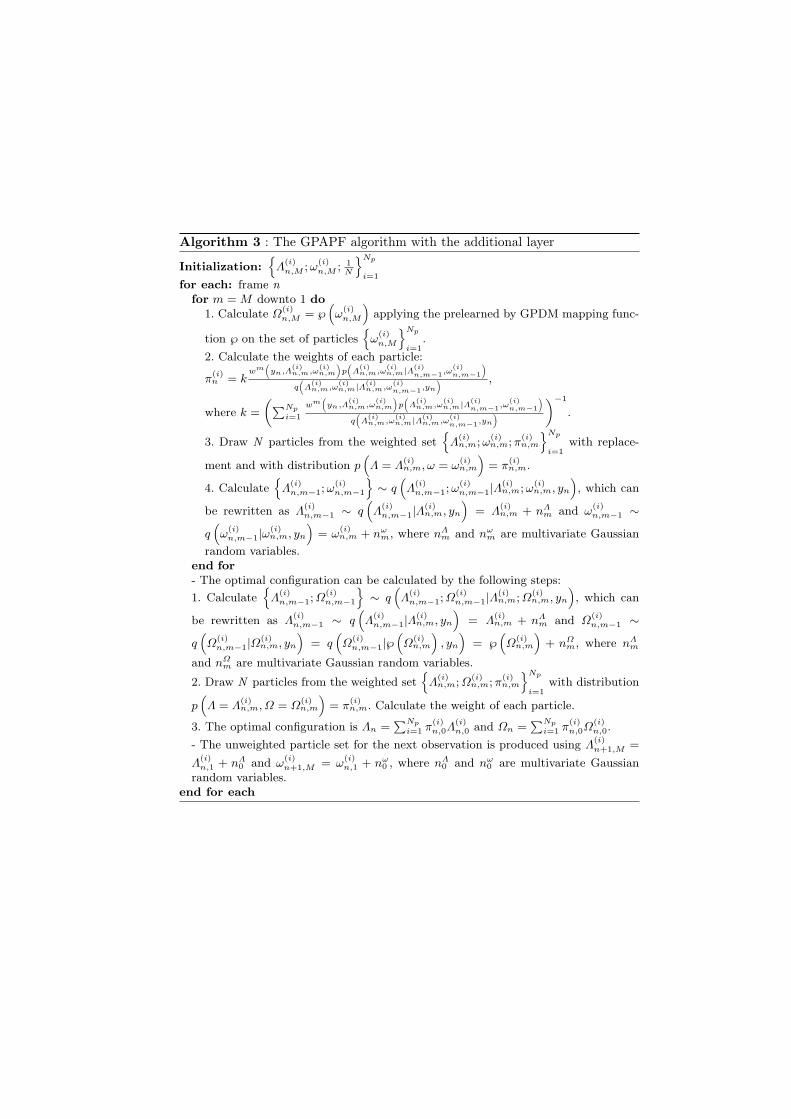
Algorithm 3 : The GPAPF algorithm with the additional layer

Initialization:

Λ(i)n,M ; ω

(i)n,M ; 1

N

Np

i=1for each: frame n

for m = M downto 1 do1. Calculate Ω

(i)n,M = ℘

(ω

(i)n,M

)applying the prelearned by GPDM mapping func-

tion ℘ on the set of particles

ω(i)n,M

Np

i=1.

2. Calculate the weights of each particle:

π(i)n = k

wm(

yn,Λ(i)n,m,ω

(i)n,m

)p(

Λ(i)n,m,ω

(i)n,m|Λ(i)

n,m−1,ω(i)n,m−1

)

q(

Λ(i)n,m,ω

(i)n,m|Λ(i)

n,m,ω(i)n,m−1,yn

) ,

where k =

(∑Np

i=1

wm(

yn,Λ(i)n,m,ω

(i)n,m

)p(

Λ(i)n,m,ω

(i)n,m|Λ(i)

n,m−1,ω(i)n,m−1

)

q(

Λ(i)n,m,ω

(i)n,m|Λ(i)

n,m,ω(i)n,m−1,yn

))−1

.

3. Draw N particles from the weighted set

Λ(i)n,m; ω

(i)n,m; π

(i)n,m

Np

i=1with replace-

ment and with distribution p(Λ = Λ

(i)n,m, ω = ω

(i)n,m

)= π

(i)n,m.

4. Calculate

Λ(i)n,m−1; ω

(i)n,m−1

∼ q

(Λ

(i)n,m−1; ω

(i)n,m−1|Λ(i)

n,m; ω(i)n,m, yn

), which can

be rewritten as Λ(i)n,m−1 ∼ q

(Λ

(i)n,m−1|Λ(i)

n,m, yn

)= Λ

(i)n,m + nΛ

m and ω(i)n,m−1 ∼

q(ω

(i)n,m−1|ω(i)

n,m, yn

)= ω

(i)n,m + nω

m, where nΛm and nω

m are multivariate Gaussian

random variables.end for- The optimal configuration can be calculated by the following steps:

1. Calculate

Λ(i)n,m−1; Ω

(i)n,m−1

∼ q

(Λ

(i)n,m−1; Ω

(i)n,m−1|Λ(i)

n,m; Ω(i)n,m, yn

), which can

be rewritten as Λ(i)n,m−1 ∼ q

(Λ

(i)n,m−1|Λ(i)

n,m, yn

)= Λ

(i)n,m + nΛ

m and Ω(i)n,m−1 ∼

q(Ω

(i)n,m−1|Ω(i)

n,m, yn

)= q

(Ω

(i)n,m−1|℘

(Ω

(i)n,m

), yn

)= ℘

(Ω

(i)n,m

)+ nΩ

m, where nΛm

and nΩm are multivariate Gaussian random variables.

2. Draw N particles from the weighted set

Λ(i)n,m; Ω

(i)n,m; π

(i)n,m

Np

i=1with distribution

p(Λ = Λ

(i)n,m, Ω = Ω

(i)n,m

)= π

(i)n,m. Calculate the weight of each particle.

3. The optimal configuration is Λn =∑Np

i=1 π(i)n,0Λ

(i)n,0 and Ωn =

∑Np

i=1 π(i)n,0Ω

(i)n,0.

- The unweighted particle set for the next observation is produced using Λ(i)n+1,M =

Λ(i)n,1 + nΛ

0 and ω(i)n+1,M = ω

(i)n,1 + nω

0 , where nΛ0 and nω

0 are multivariate Gaussianrandom variables.

end for each

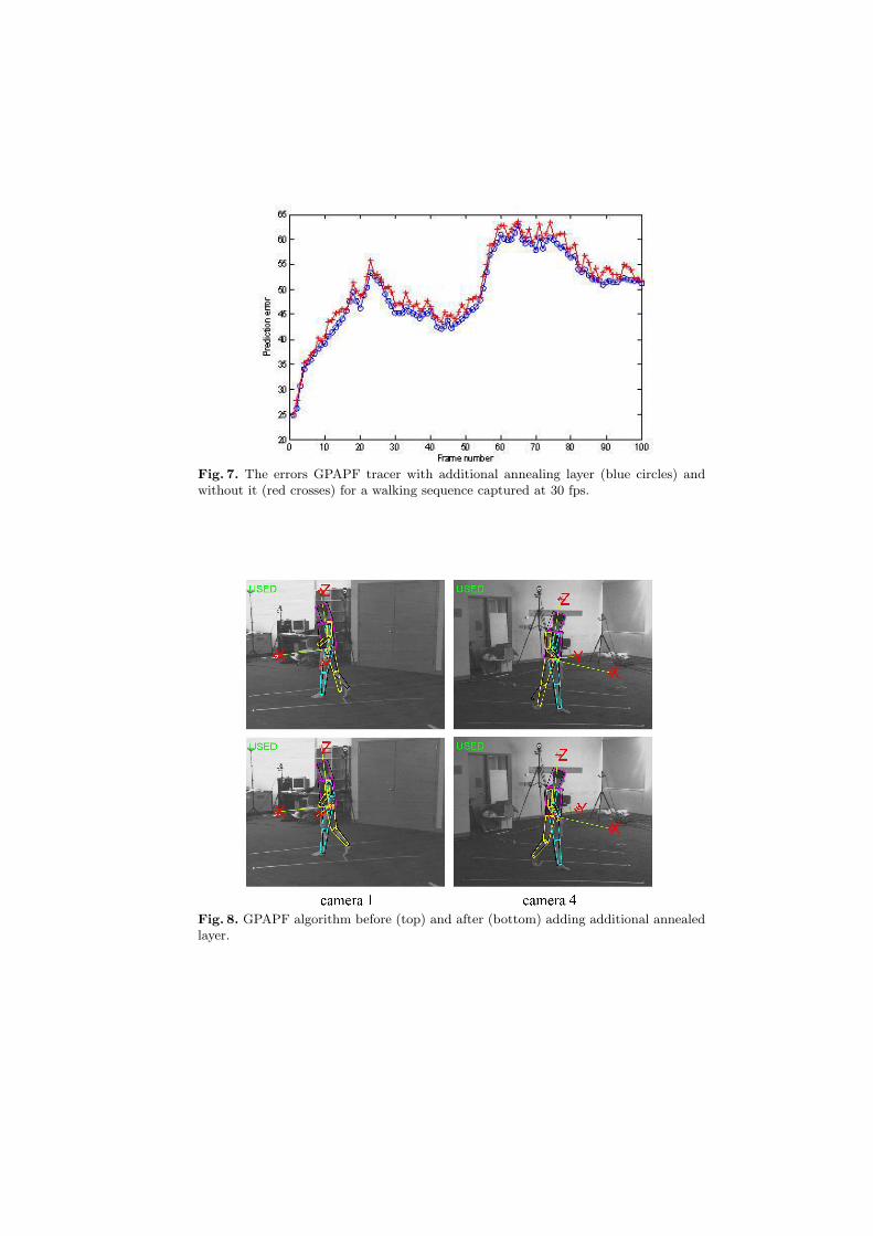
Fig. 7. The errors GPAPF tracer with additional annealing layer (blue circles) andwithout it (red crosses) for a walking sequence captured at 30 fps.

Fig. 8. GPAPF algorithm before (top) and after (bottom) adding additional annealedlayer.

particles. As we have seen from our experiments, there are often many particleswith the weight close to the optimal. Therefore, the result is less sensitive to thelocation of some particular particle. It depends on the whole set of them.

We have also tried to use the results, produced by the additional layer, inorder to initialize the state in the next time step. This was done by applyingthe inverse function ℘−1, suggested by Lawrence [8], on the particles that weregenerated in previous annealing layer. However, this approach did not produceany valuable improvement in the tracking results. As the inverse function is com-putationally heavy it caused significant increase the calculation time. Therefore,we decided not to experiment with it further.

6 Results

We have tested GPAPF tracking algorithm using HumanEva dataset [22]. Thesequences contain different activities, such as walking, boxing etc. which werecaptured by 7 cameras; however we have used only 4 inputs in our evaluation.The sequences were captured using the MoCap system that provides the correct3D locations of the body parts for evaluation of the results and comparison toother tracking algorithms.

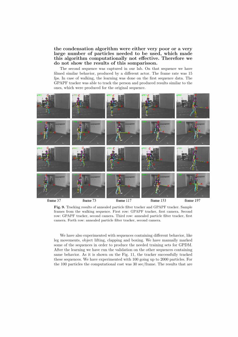
The first sequence that we have used was a walk on a circle. The videowas captured at frame rate 120 fps. We have tested the annealed particle filterbased body tracker, implemented by A. Balan, and compared the results withthe ones produced by the GPAPF tracker. The error was calculated, based oncomparison of the tracker’s output and the result of the MoCap system, usingaverage distance between 3-D joints location, as explained in section 5.4. Fig. 10shows the error graphs, produced by GPAPF tracker (blue circles) and by theannealed particle filter (red crosses) for the walking sequence taken at 30 fps. Ascan be seen, the GPAPF tracker produces more accurate estimation of the bodylocation. Same results were achieved for 15 fps. Fig. 9 presents sample imageswith the actual pose estimation for this sequence. The poses are projected tothe first and second cameras. The first 2 rows show the results of the GPAPFtracker. The third and forth rows show the results of the annealed particle filter.

We have experimented with 100 particles up to 2000 par-ticles. For the 100 particles per layer using 5 annealed lay-ers the computational cost was 30 sec per frame. Using thesame number of particles and layers in the annealed particlefilter algorithm takes 20 seconds per frame. However, theannealed particle filter algorithm was not capable of track-ing the body pose with such a low number of particles for30 fps and 15 fps videos. Therefore, we had to increase thenumber of particles used in the annealed particle filter to500.

We have also tried to compare our results to the resultsof CONDENSATION algorithm. However, the results of

the condensation algorithm were either very poor or a verylarge number of particles needed to be used, which madethis algorithm computationally not effective. Therefore wedo not show the results of this somparisson.

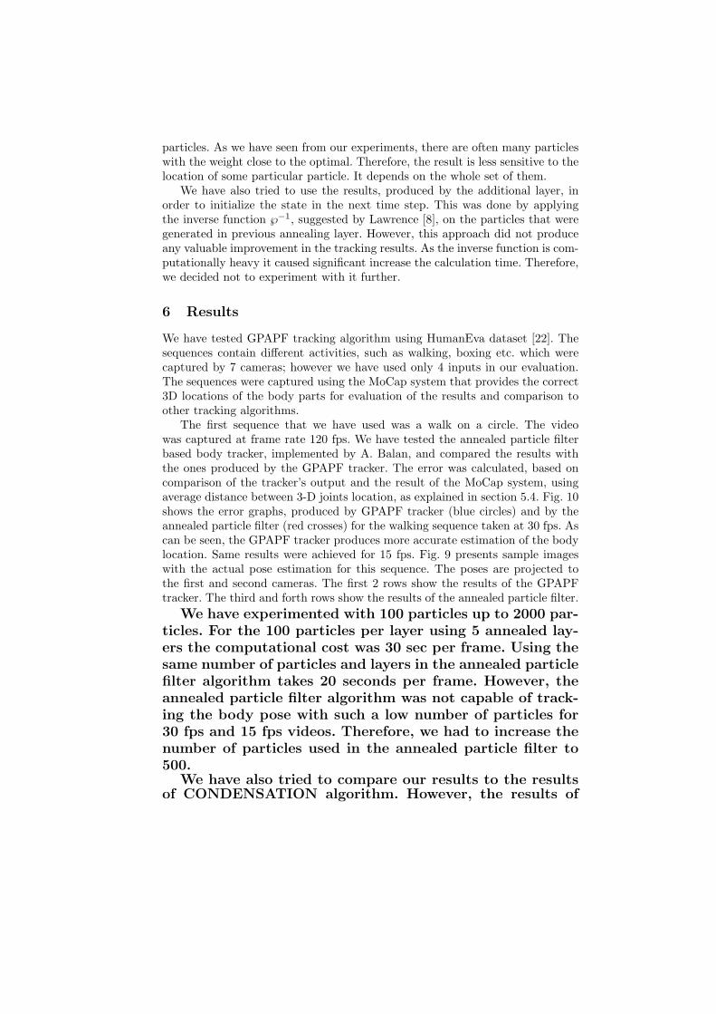
The second sequence was captured in our lab. On that sequence we havefilmed similar behavior, produced by a different actor. The frame rate was 15fps. In case of walking, the learning was done on the first sequence data. TheGPAPF tracker was able to track the person and produced results similar to theones, which were produced for the original sequence.

Fig. 9. Tracking results of annealed particle filter tracker and GPAPF tracker. Sampleframes from the walking sequence. First row: GPAPF tracker, first camera. Secondrow: GPAPF tracker, second camera. Third row: annealed particle filter tracker, firstcamera. Forth row: annealed particle filter tracker, second camera.

We have also experimented with sequences containing different behavior, likeleg movements, object lifting, clapping and boxing. We have manually markedsome of the sequences in order to produce the needed training sets for GPDM.After the learning we have run the validation on the other sequences containingsame behavior. As it is shown on the Fig. 11, the tracker successfully trackedthese sequences. We have experimented with 100 going up to 2000 particles. Forthe 100 particles the computational cost was 30 sec/frame. The results that are

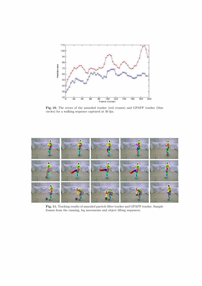
Fig. 10. The errors of the annealed tracker (red crosses) and GPAPF tracker (bluecircles) for a walking sequence captured at 30 fps.

Fig. 11. Tracking results of annealed particle filter tracker and GPAPF tracker. Sampleframes from the running, leg movements and object lifting sequences.

shown in the videos are done with 500 particles (2.5 min per frame). The codethat we are using is written in Matlab with no optimization packages. Thereforethe computational cost can be significantly reduced if moved to C libraries.

7 Conclusion and Future Work

We have presented an approach that uses GPDM in order to reduce the dimen-sionality and in this way to improve the ability of the annealed particle filtertracker to track the object even in a high dimensional space. We have also shownthat using GPDM can increase the ability to recover from temporal target loss.We have also presented a method to approximate the possibility of self occlusionand we have suggested a way to adjust the weighed function for such cases, inorder to be able to produce more accurate evaluation of a pose.

The main problem is that the learning and tracking are done for a specificaction. The ability of the tracker to use a latent space in order to track a differentmotion type, has not been shown yet. A possible approach is to construct acommon latent space for the poses from different actions. The difficulty withsuch approach may be the presence of a large number of gaps between theconsecutive poses. In the future we plan to extend the approach in order to beable to track different activities, using same learned data.

The other challenging task is to track two or more people simultaneously.The main problem here is that in this case there is high possibility of occlusion.Furthermore, while for a single person each body part can be seen from at leastone camera that is not the case for the crowded scenes.

References

1. Agarwal A. and Triggs B. 3d human pose from silhouettes by relevance vectorregression. Proc. CVPR, 2:882–888, 2004.

2. Agarwal A. and Triggs B. Learning to track 3d human motion from silhouettes.Proc. ICML, page 916, 2004.

3. Deutscher J. Blake A. and Reid I. Articulated body motion capture by annealedparticle filtering. Proc. CVPR, pages 2126–2133, 2000.

4. Elgammal A.M. and Lee C. Inferring 3d body pose from silhouettes using activitymani-fold learning. Proc. CVPR, 2:681–688, 2004.

5. A. Sigal L. Balan and Black. M. A quantitative evaluation of video-based 3d persontracking. IEEE Workshop on Visual Surveillance and Performance Evaluation ofTracking and Surveillance (VS-PETS), pages 349–356, 2005.

6. Bregler C. and Malik J. Tracking people with twists and exponential maps. Proc.CVPR, pages 8–15, 1998.

7. Lawrence N. D. Gaussian process latent variable models for visualization of highdimensional data. Information Processing Systems (NIPS), 16:329–336, 2004.

8. Lawrence N. D. and Candela J. Q. Local distance preservation in the gp-lvmthrough back constraints. Proc. International Conference on Machine Learning(ICML), pages 513–520, 2006.

9. Ramanan D. and Forsyth D. A. Automatic annotation of everyday movements.Information Processing Systems (NIPS), 2003.

10. Tenenbaum J. B. de Silva and V. Langford. J.C. A global geometric frameworkfor nonlinear dimensionality reduction. Science, 290:2319–2323, 2000.

11. Raskin L. Rivlin E. and Rudzsky M. 3d human tracking with gaussian processannealed particle. Proc. VISAPP, pages 661–675, 2007.

12. Mori G. and Malik J. Estimating human body configurations using shape contextmatching. Proc. ECCV, 3:134–141, 2002.

13. Wang Q. Xu G. and Ai H. Learning object intrinsic structure for robust visualtracking. Proc. CVPR, 2:227–233, 2003.

14. Davison A. J. Deutscher J. and Reid I. D. Markerless motion capture of com-plex full-body movement for character animation. In Eurographics Workshop onComputer Anima-tion and Simulation, pages 3–14, 2001.

15. Deutscher J. and Reid I. Articulated body motion capture by stochastic search.International Journal of Computer Vision, 61(2):185–205, 2004.

16. Perez P. Hue C. Vermaak J. and Gangnet M. Color-based probabilistic tracking.Proc. ECCV, pages 661–675, 2002.

17. Sidenbladh H. Black M. J. and Sigal L. Implicit probabilistic models of humanmotion for synthesis and tracking. Proc. ECCV, 1:784–800, 2002.

18. Urtasun R. Fleet D. J. and Fua P. 3d people tracking with gaussian processdynamical models. Proc. CVPR, 1:238–245, 2006.

19. Wang J. Fleet D. J. and Hetzmann A. Gaussian process dynamical models. Infor-mation Processing Systems (NIPS), pages 1441–1448, 2005.

20. Mikolajczyk K. Schmid K. and Zisserman. A. Human detection based on a prob-abilistic assembly of robust part detectors. Proc. ECCV, 1:69–82, 2003.

21. Rohr K. Human movement analysis based on explicit motion models. Motion-Based Recognition, 8:171–198, 1997.

22. Sigal L. and Black M.J. Humaneva: Cynchronized video and motion capturedataset for evaluation of articulated human motion. Technical Report CS-06-08,2006.

23. Isard M. and Blake A. Condensation - conditional density propagation for visualtracking. International Journal of Computer Vision, 29(1):5–28, 1998.

24. Isard M. and MacCormick J. Bramble: A bayesian multiple blob tracker. Proc.ICCV, pages 34–41, 2001.

25. Ormoneit D. Sidenbladh H. Black M. and Hastie T. Learning and tracking cyclichuman motion. Advances in Neural Information Processing Systems, 13:894–900,2001.

26. Raskin L. Rudzsky M. and Rivlin E. Gpapf: A combined approach for 3d bodypart tracking. Proc. ICVS, 2007.

27. Sidenbladh H. Black M. and Fleet D. Stochastic tracking of 3d human figures using2d image motion. Proc. ECCV, 2:702–718, 2000.

28. Urtasun R. Fleet D.J. Hertzmann A. Fua P. Priors for people tracking from smalltraining sets. Proc. ICCV, 1:403–410, 2005.

29. Urtasun R. and Fua P. 3d human body tracking using deterministic temporalmotion models. Proc. ECCV, 3:92–106, 2004.

30. Ioffe S. and Forsyth. D. A. Human tracking with mixtures of trees. Proc. ICCV,1:690–695, 2001.

31. Roweis S. T. and Saul L. K. Nonlinear dimensionality reduction by locally linearembedding. Science, 290:2323–2326, 2000.

32. Comaniciu D. Ramesh V. and Meer P. Kernel-based object tracking. IEEE Trans.PAMI, 25(5):564–577, 2003.

33. Song Y. Feng X. and Perona P. Towards detection of human motion. Proc. CVPR,pages 810–817, 2000.