1/18

Parameter Estimation in Non-Gaussian State-Space Models using

Particle Methods and the EM Algorithm

Amanda Halladay

Department of Mathematics and Statistics

Dalhousie University

October 15, 2006

1/18

Motivation

• State-space models gaining popularity

• Allow for outlying observations

• Vast and Inexpensive Computational Methods

• Circle of Confusion Model

2/18

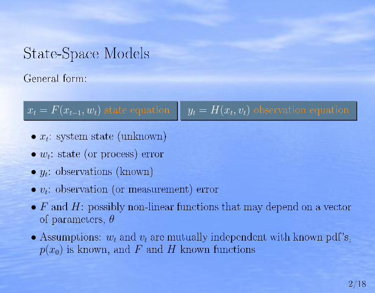
State-Space Models

General form:

xt = F (xt−1, wt) state equation yt = H(xt, vt) observation equation

• xt: system state (unknown)

• wt: state (or process) error

• yt: observations (known)

• vt: observation (or measurement) error

• F and H: possibly non-linear functions that may depend on a vectorof parameters, θ

• Assumptions: wt and vt are mutually independent with known pdf's,p(x0) is known, and F and H known functions

3/18

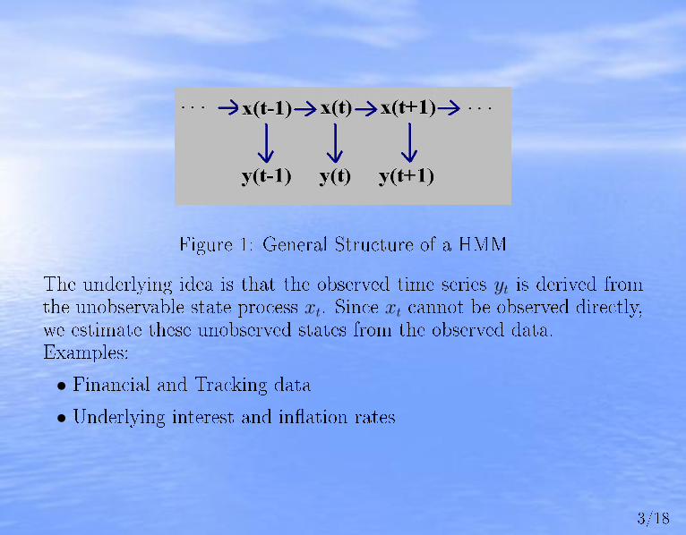
Figure 1: General Structure of a HMM

The underlying idea is that the observed time series yt is derived fromthe unobservable state process xt. Since xt cannot be observed directly,we estimate these unobserved states from the observed data.Examples:

• Financial and Tracking data

• Underlying interest and in�ation rates

4/18

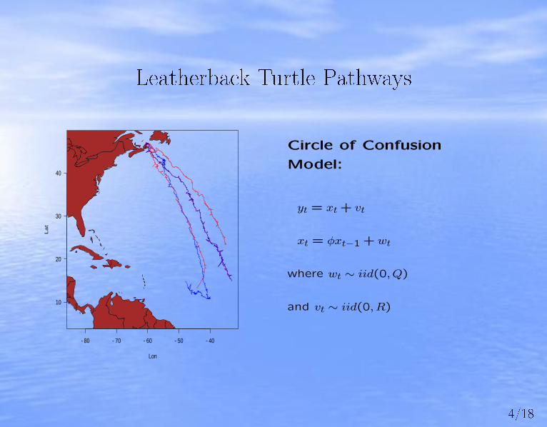
Leatherback Turtle Pathways

−80 −70 −60 −50 −40

10

20

30

40

Lon

La

t

Circle of Confusion

Model:

yt = xt + vt

xt = φxt−1 + wt

where wt ∼ iid(0, Q)

and vt ∼ iid(0, R)

5/18

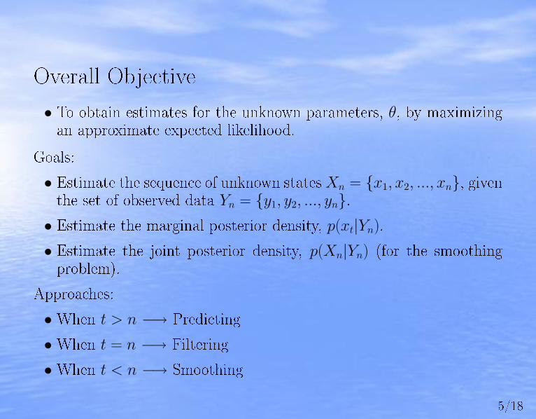
Overall Objective

• To obtain estimates for the unknown parameters, θ, by maximizingan approximate expected likelihood.

Goals:

• Estimate the sequence of unknown states Xn = {x1, x2, ..., xn}, giventhe set of observed data Yn = {y1, y2, ..., yn}.

• Estimate the marginal posterior density, p(xt|Yn).

• Estimate the joint posterior density, p(Xn|Yn) (for the smoothingproblem).

Approaches:

• When t > n −→ Predicting

• When t = n −→ Filtering

• When t < n −→ Smoothing

6/18

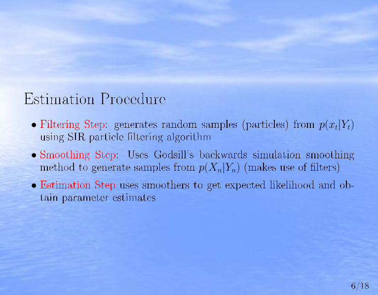
Estimation Procedure

• Filtering Step: generates random samples (particles) from p(xt|Yt)using SIR particle �ltering algorithm

• Smoothing Step: Uses Godsill's backwards simulation smoothingmethod to generate samples from p(Xn|Yn) (makes use of �lters)

• Estimation Step uses smoothers to get expected likelihood and ob-tain parameter estimates

7/18

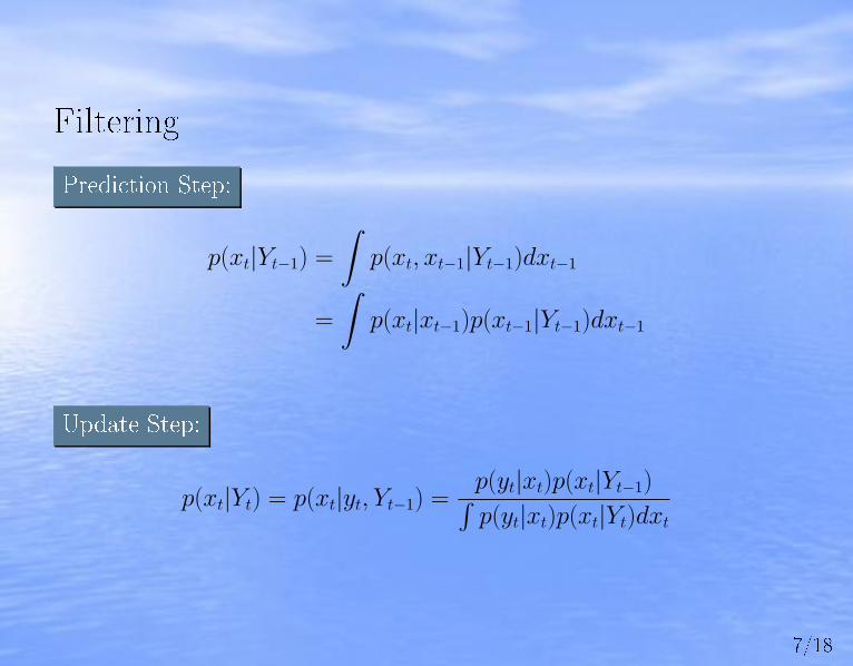
Filtering

Prediction Step:

p(xt|Yt−1) =

∫p(xt, xt−1|Yt−1)dxt−1

=

∫p(xt|xt−1)p(xt−1|Yt−1)dxt−1

Update Step:

p(xt|Yt) = p(xt|yt, Yt−1) =p(yt|xt)p(xt|Yt−1)∫p(yt|xt)p(xt|Yt)dxt

8/18

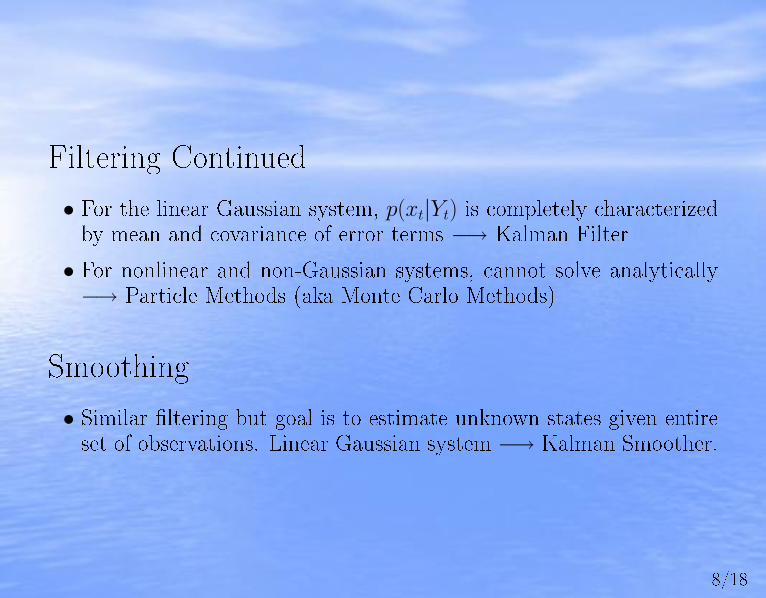
Filtering Continued

• For the linear Gaussian system, p(xt|Yt) is completely characterizedby mean and covariance of error terms −→ Kalman Filter

• For nonlinear and non-Gaussian systems, cannot solve analytically−→ Particle Methods (aka Monte Carlo Methods)

Smoothing

• Similar �ltering but goal is to estimate unknown states given entireset of observations. Linear Gaussian system −→ Kalman Smoother.

9/18

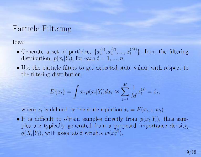
Particle Filtering

Idea:

• Generate a set of particles, {x(1)t , x

(2)t , ..., x

(M)t }, from the �ltering

distribution, p(xt|Yt), for each t = 1, ..., n.

• Use the particle �lters to get expected state values with respect tothe �ltering distribution:

E{xt} =

∫xt p(xt|Yt)dxt ≈

M∑j=1

1

Mx

(j)t = x̂t,

where xt is de�ned by the state equation xt = F (xt−1, wt).

• It is di�cult to obtain samples directly from p(xt|Yt), thus sam-ples are typically generated from a proposed importance density,q(Xt|Yt), with associated weights w(x

(j)t ).

10/18

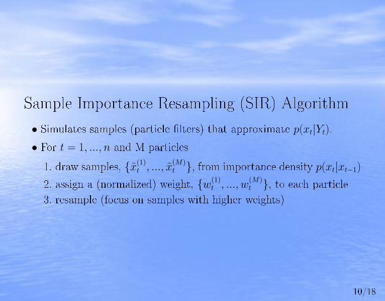
Sample Importance Resampling (SIR) Algorithm

• Simulates samples (particle �lters) that approximate p(xt|Yt).

• For t = 1, ..., n and M particles

1. draw samples, {x̃(1)t , ..., x̃

(M)t }, from importance density p(xt|xt−1)

2. assign a (normalized) weight, {w(1)t , ..., w

(M)t }, to each particle

3. resample (focus on samples with higher weights)

11/18

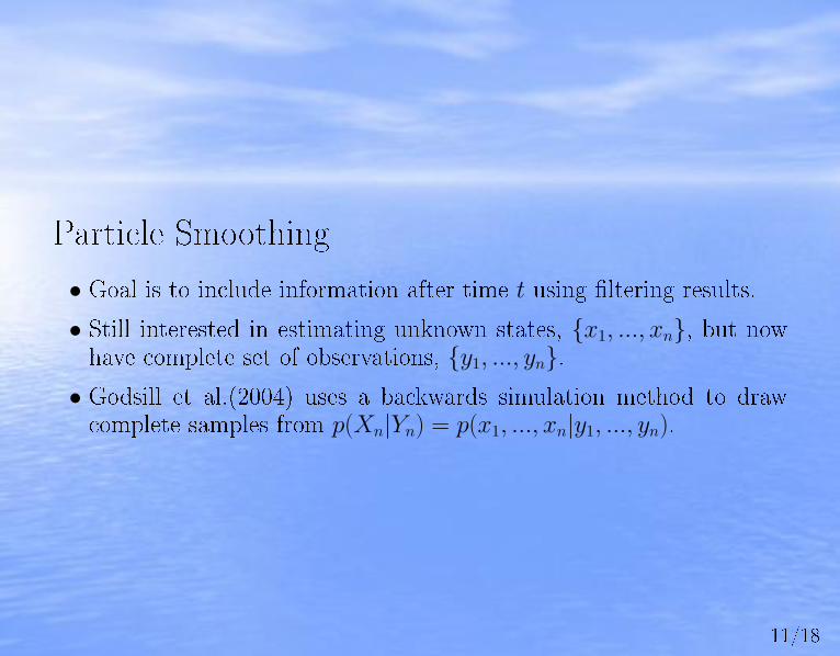
Particle Smoothing

• Goal is to include information after time t using �ltering results.

• Still interested in estimating unknown states, {x1, ..., xn}, but nowhave complete set of observations, {y1, ..., yn}.

• Godsill et al.(2004) uses a backwards simulation method to drawcomplete samples from p(Xn|Yn) = p(x1, ..., xn|y1, ..., yn).

12/18

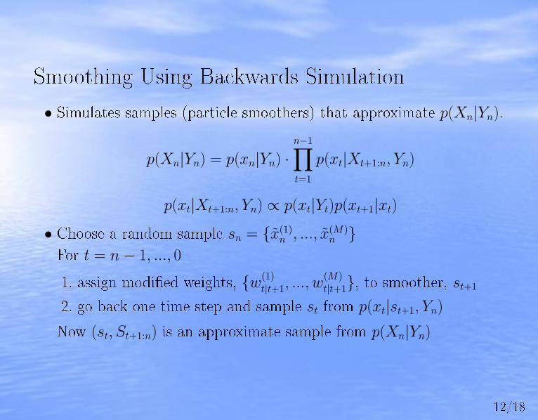
Smoothing Using Backwards Simulation

• Simulates samples (particle smoothers) that approximate p(Xn|Yn).

p(Xn|Yn) = p(xn|Yn) ·n−1∏t=1

p(xt|Xt+1:n, Yn)

p(xt|Xt+1:n, Yn) ∝ p(xt|Yt)p(xt+1|xt)

• Choose a random sample sn = {x̃(1)n , ..., x̃(M)

n }For t = n− 1, ..., 0

1. assign modi�ed weights, {w(1)t|t+1, ..., w

(M)t|t+1}, to smoother, st+1

2. go back one time step and sample st from p(xt|st+1, Yn)

Now (st, St+1:n) is an approximate sample from p(Xn|Yn)

13/18

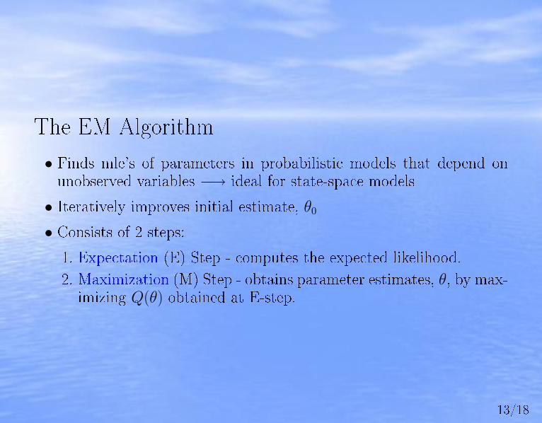
The EM Algorithm

• Finds mle's of parameters in probabilistic models that depend onunobserved variables −→ ideal for state-space models

• Iteratively improves initial estimate, θ0

• Consists of 2 steps:

1. Expectation (E) Step - computes the expected likelihood.

2. Maximization (M) Step - obtains parameter estimates, θ, by max-imizing Q(θ) obtained at E-step.

14/18

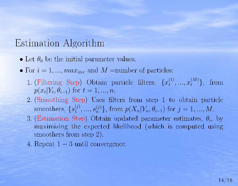
Estimation Algorithm

• Let θ0 be the initial parameter values.

• For i = 1, ...,maxiter and M =number of particles:

1. (Filtering Step) Obtain particle �lters, {x(1)t , ..., x

(M)t }, from

p(xt|Yt, θi−1) for t = 1, ..., n.

2. (Smoothing Step) Uses �lters from step 1 to obtain particle

smoothers, {s(j)1 , ..., s(j)

n }, from p(Xn|Yn, θi−1) for j = 1, ...,M .

3. (Estimation Step) Obtain updated parameter estimates, θi, bymaximizing the expected likelihood (which is computed usingsmoothers from step 2).

4. Repeat 1− 3 until convergence.

15/18

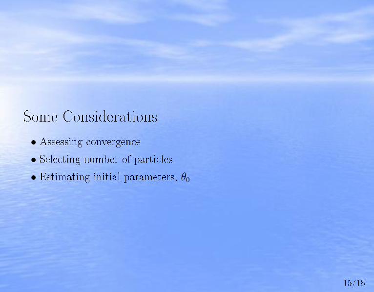
Some Considerations

• Assessing convergence

• Selecting number of particles

• Estimating initial parameters, θ0

16/18

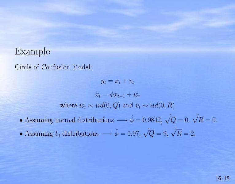
Example

Circle of Confusion Model:

yt = xt + vt

xt = φxt−1 + wt

where wt ∼ iid(0, Q) and vt ∼ iid(0, R)

• Assuming normal distributions −→ φ̂ = 0.9842,√̂

Q = 0,√̂

R = 0.

• Assuming t3 distributions −→ φ̂ = 0.97,√̂

Q = 9,√̂

R = 2.

17/18

Future Research

• Improving computational speed?

• Improving estimate of initial parameters

• Missing data

18/18

References

J.E. Mills-Flemming, C.A. Field, M.C. James, I.D, Jonsen, and R.A.Myers. How Well Can Animals Navigate? Estimating the Circle ofConfusion from Satellite Telemetry. Environmetrics, 17(4), 2006.

S.J. Godsill, A. Doucet, and M. West. Monte Carlo Smooting for Non-linear Time Series. Journal of the American Statistical Association,99(465), March 2004.

Jeongeun Kim. Parameter Estimation in Stochastic Volatility Modelswith Missing Data Using Particle Methods and the EM Algorithm. PhDthesis, University of Pittsburgh, 2005.

Genshiro Kitagawa. Monte Carlo Filter an Smoother for Non-GaussianNon-linear State Space Models. 1996.