Using Confidence Intervals for Graphically Based Data Interpretation

Canadian Journal of Experimental Psychology, (2003), in press

Using Confidence Intervals for GraphicallyBased Data Interpretation

MICHAEL E. J. MASSON, University of VictoriaGEOFFREY R. LOFTUS, University of Washington

Abstract As a potential alternative to standard nullhypothesis significance testing, we describe methodsfor graphical presentation of data––particularly condi-tion means and their corresponding confidence inter-vals––for a wide range of factorial designs used in ex-perimental psychology. We describe and illustrate con-fidence intervals specifically appropriate for between-subject versus within-subject factors. For designs in-volving more than two levels of a factor, we describethe use of contrasts for graphical illustration of theo-retically meaningful components of main effects andinteractions. These graphical techniques lend them-selves to a natural and straightforward assessment ofstatistical power.

Null hypothesis significance testing (NHST), althoughhotly debated in the psychological literature on statisti-cal analysis (e.g., Chow, 1998; Cohen, 1990, 1994;Hagen, 1997; Hunter, 1997; Lewandowsky & Maybery,1998; Loftus, 1991, 1993, 1996, 2002; Schmidt, 1996),is not likely to go away any time soon (Krueger, 2001).Generations of students from multiple disciplines con-tinue to be schooled in the NHST approach to inter-preting empirical data, and practicing scientists relyalmost reflexively on the logic and methods associatedwith it. Our goal here is not to extend this debate, butrather to enhance understanding of a particular alterna-tive to NHST for interpreting data. In our view, to the

extent that a variety of informative means of construct-ing inferences from data are made available and clearlyunderstood, researchers will increase their likelihood offorming appropriate conclusions and communicatingeffectively with their audiences.

A number of years ago, we advocated and de-scribed computational approaches to the use of confi-dence intervals as part of a graphical approach to datainterpretation (Loftus & Masson, 1994; see also, Loftus,2002). The power and effectiveness of graphical datapresentation is undeniable (Tufte, 1983) and is commonin all forms of scientific communication in experimen-tal psychology and in other fields. In many instances,however, plots of descriptive statistics (typicallymeans) are not accompanied by any indication of vari-ability or stability associated with those descriptivestatistics. The diligent reader, then, is forced to refer toa dreary accompanying recital of significance tests todetermine how the pattern of means should be inter-preted.

It has become clear through interactions with col-leagues and from queries we have received about theuse of confidence intervals in conjunction with graphi-cal presentation of data, that more information isneeded about practical, computational steps involved ingenerating confidence intervals, particularly with re-spect to designs involving interactions among variables.In this article, we briefly explain the logic behind con-fidence intervals for both between-subject and within-subject designs, then move to a consideration of a rangeof multifactor designs wherein interaction effects are ofinterest. Methods for computing and displaying confi-dence intervals for a variety of between-subject, within-subject, and mixed designs commonly used in experi-mental psychology are illustrated with hypothetical datasets. These descriptions go beyond the range of experi-mental designs considered in Loftus and Masson(1994). Moreover, we extend the use of contrasts dis-cussed by Loftus (2002) and present a method for using

Preparation of this report was supported by Discovery GrantA7910 from the Natural Sciences and Engineering ResearchCouncil of Canada to Michael Masson and by U.S. NationalInstitute of Mental Health grant MH41637 to GeoffreyLoftus. We thank Stephen Lindsay, Raymond Nickerson,and Warren Tryon for helpful comments on an earlier ver-sion of this paper.Correspondence to: Michael Masson, Department of Psy-chology, University of Victoria, PO Box 3050 STN CSC,Victoria BC V8W 3P5, Canada. e-mail: [email protected]

2 Masson and Loftus

planned contrasts to examine theoretically motivatedeffects generated by factorial designs. Finally, we con-sider an additional, crucial advantage of this graphicalapproach to data interpretation that is sorely lacking instandard applications of NHST, namely, the ease withwhich one can assess an experiment's statistical power.

Interpretation of Confidence IntervalsThe formal interpretation of a confidence interval

associated with a sample mean is based on the hypo-thetical situation in which many random samples aredrawn from a population. For each such sample, themean, standard deviation, and sample size are used toconstruct a confidence interval representing a specifieddegree of confidence, say 95%. Thus, for each samplewe have

95%CI = M ± SEM (t95%) (1)

Under these conditions, it is expected that 95% ofthese sample-specific confidence intervals will includethe population mean. In practical situations, however,we typically have only one sample from a specifiedpopulation (e.g., an experimental condition) and there-fore the interpretation of the confidence interval con-structed around that specific mean would be that thereis a 95% probability that the interval is one of the 95%of all possible confidence intervals that includes thepopulation mean. Put more simply, in the absence ofany other information, there is a 95% probability thatthe obtained confidence interval includes the populationmean.

The goal of designing a sensitive experiment is toobtain precise and reliable measurements that are con-taminated by as little measurement error as possible. Tothe extent that a researcher accomplishes this goal, theconfidence intervals constructed around sample meanswill be relatively small, allowing the researcher accu-rately to infer the corresponding pattern of populationmeans. That is, inferences about patterns of populationmeans and the relations among these means can be de-rived from the differences among sample means, rela-tive to the size of their associated confidence intervals.

Confidence Intervals forBetween-Subject Designs

The construction and interpretation of confidenceintervals is most directly appropriate to designs inwhich independent groups of subjects are assigned toconditions––the between-subject design. To illustratethe use of confidence intervals in this context, considera study in which different groups of subjects are as-signed to different conditions in a study of selective

attention involving Stroop stimuli. Admittedly, this isthe kind of experiment more likely to be conductedusing a repeated-measures or within-subject design, butwe will carry this example over to that context below.Assume that one group of subjects is shown a series ofcolor words (e.g., blue, green), each appearing in anincongruent color (e.g., the word blue printed in thecolor green). The task is to name the color as quickly aspossible. A second group is shown a series of colorwords, each printed in a congruent color (e.g., the wordblue printed in the color blue), and a third group isshown a series of consonant strings (e.g., kfgh, trnds,etc.), each printed in one of the target colors.

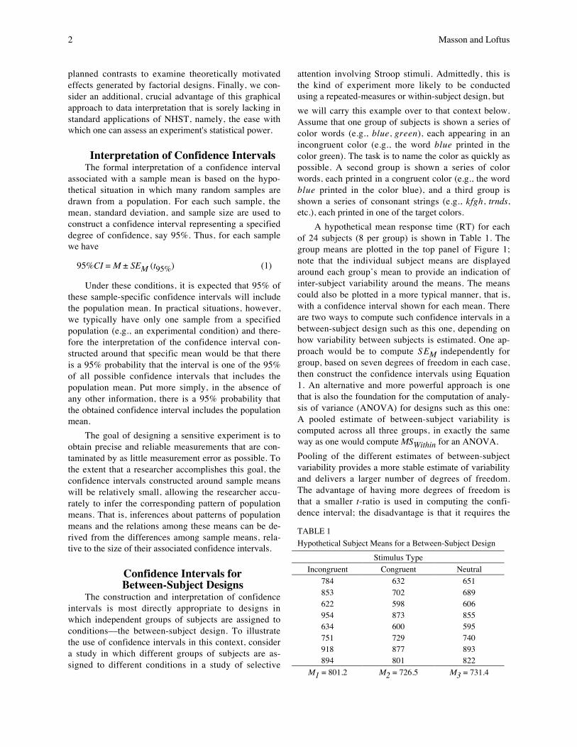
A hypothetical mean response time (RT) for eachof 24 subjects (8 per group) is shown in Table 1. Thegroup means are plotted in the top panel of Figure 1;note that the individual subject means are displayedaround each group’s mean to provide an indication ofinter-subject variability around the means. The meanscould also be plotted in a more typical manner, that is,with a confidence interval shown for each mean. Thereare two ways to compute such confidence intervals in abetween-subject design such as this one, depending onhow variability between subjects is estimated. One ap-proach would be to compute S EM independently forgroup, based on seven degrees of freedom in each case,then construct the confidence intervals using Equation1. An alternative and more powerful approach is onethat is also the foundation for the computation of analy-sis of variance (ANOVA) for designs such as this one:A pooled estimate of between-subject variability iscomputed across all three groups, in exactly the sameway as one would compute MSWithin for an ANOVA.Pooling of the different estimates of between-subjectvariability provides a more stable estimate of variabilityand delivers a larger number of degrees of freedom.The advantage of having more degrees of freedom isthat a smaller t-ratio is used in computing the confi-dence interval; the disadvantage is that it requires the

TABLE 1Hypothetical Subject Means for a Between-Subject Design

Stimulus TypeIncongruent Congruent Neutral

784 632 651853 702 689622 598 606954 873 855634 600 595751 729 740918 877 893894 801 822

M1 = 801.2 M2 = 726.5 M3 = 731.4

Confidence Intervals 3

homogeneity of variance assumption, i.e., the assump-tion that the population variance is the same in allgroups (we return to this issue below). In any event,using the pooled estimate of variability results in thefollowing general equation for confidence intervals inthe between-subject design:

CI = Mj ±

†

MSWithin

nj

(tcritical) (2)

where Mj is the mean for and nj is the number of sub-jects in Group j. Note that when the n’s in the differentgroups are the same, as is true in our example, a single,common confidence interval can be produced and plot-ted around each of the group means.

To produce a graphic presentation of the meansfrom this hypothetical study, then, we can computeMSWithin using an ANOVA program, then construct theconfidence interval to be used with each mean usingEquation 2. The MSWithin for these data is 14,054 (seeFigure 1). With 21 degrees of freedom, the critical t-ratio for a 95% confidence interval is 2.080 and n = 8,so the confidence interval is computed from Equation 2to be ±87.18. The resulting plot of the three groupmeans and their associated 95% confidence interval isshown in the lower panel of Figure 1. It is clear fromthe size of the confidence interval that these data do notimply strong differences between the three groups. In-deed, the ANOVA computed for the purpose of ob-taining MSWithin generated an F-ratio of 1.00, clearlynot significant by conventional NHST standards.

Confidence Intervals forWithin-Subject Designs

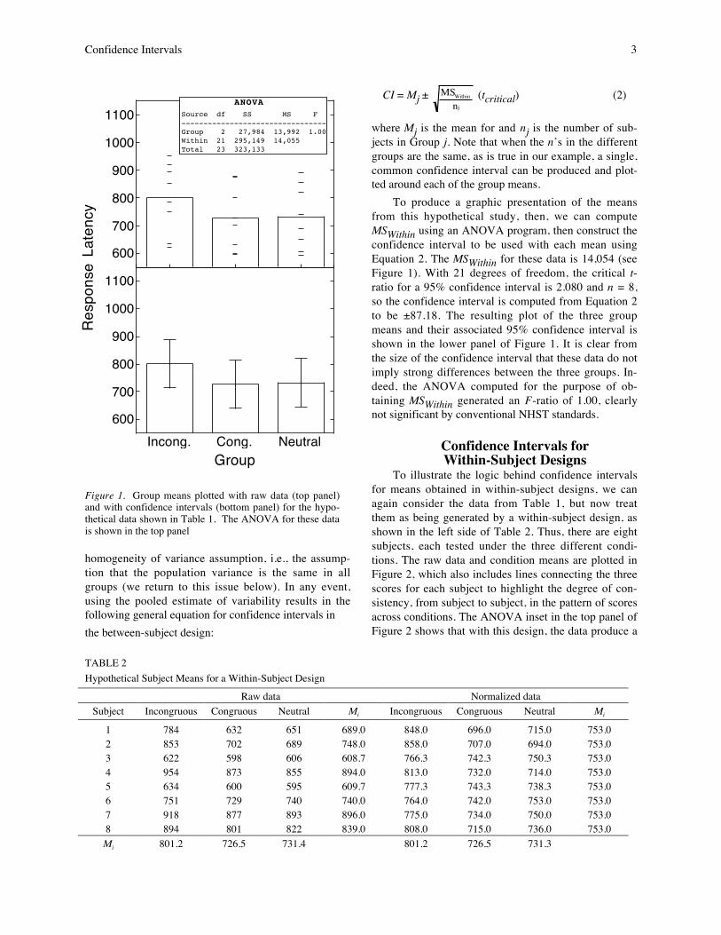
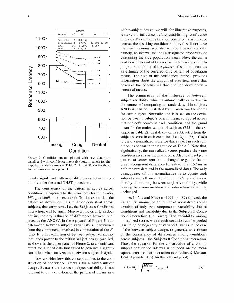
To illustrate the logic behind confidence intervalsfor means obtained in within-subject designs, we canagain consider the data from Table 1, but now treatthem as being generated by a within-subject design, asshown in the left side of Table 2. Thus, there are eightsubjects, each tested under the three different condi-tions. The raw data and condition means are plotted inFigure 2, which also includes lines connecting the threescores for each subject to highlight the degree of con-sistency, from subject to subject, in the pattern of scoresacross conditions. The ANOVA inset in the top panel ofFigure 2 shows that with this design, the data produce a

TABLE 2Hypothetical Subject Means for a Within-Subject Design

Raw data Normalized dataSubject Incongruous Congruous Neutral Mi Incongruous Congruous Neutral Mi

1 784 632 651 689.0 848.0 696.0 715.0 753.02 853 702 689 748.0 858.0 707.0 694.0 753.03 622 598 606 608.7 766.3 742.3 750.3 753.04 954 873 855 894.0 813.0 732.0 714.0 753.05 634 600 595 609.7 777.3 743.3 738.3 753.06 751 729 740 740.0 764.0 742.0 753.0 753.07 918 877 893 896.0 775.0 734.0 750.0 753.08 894 801 822 839.0 808.0 715.0 736.0 753.0Mj 801.2 726.5 731.4 801.2 726.5 731.3

Figure 1. Group means plotted with raw data (top panel)and with confidence intervals (bottom panel) for the hypo-thetical data shown in Table 1. The ANOVA for these datais shown in the top panel

600

700

800

900

1000

1100

Incong. Cong. Neutral

Res

pons

e La

tenc

y

Group

600

700

800

900

1000

1100 ANOVASource df SS MS F---------------------------------Group 2 27,984 13,992 1.00Within 21 295,149 14,055Total 23 323,133

4 Masson and Loftus

clearly significant pattern of differences between con-ditions under the usual NHST procedures.

The consistency of the pattern of scores acrossconditions is captured by the error term for the F-ratio,MSSXC (1,069 in our example). To the extent that thepattern of differences is similar or consistent acrosssubjects, that error term, i.e., the Subjects x Conditionsinteraction, will be small. Moreover, the error term doesnot include any influence of differences between sub-jects, as the ANOVA in the top panel of Figure 2 indi-cates––the between-subject variability is partitionedfrom the components involved in computation of the F-ratio. It is this exclusion of between-subject variabilitythat lends power to the within-subject design (and led,as shown in the upper panel of Figure 2, to a significanteffect for a set of data that failed to generate a signifi-cant effect when analyzed as a between-subject design).

Now consider how this concept applies to the con-struction of confidence intervals for a within-subjectdesign. Because the between-subject variability is notrelevant to our evaluation of the pattern of means in a

within-subject design, we will, for illustrative purposes,remove its influence before establishing confidenceintervals. By excluding this component of variability, ofcourse, the resulting confidence interval will not havethe usual meaning associated with confidence intervals,namely, an interval that has a designated probability ofcontaining the true population mean. Nevertheless, aconfidence interval of this sort will allow an observer tojudge the reliability of the pattern of sample means asan estimate of the corresponding pattern of populationmeans. The size of the confidence interval providesinformation about the amount of statistical noise thatobscures the conclusions that one can draw about apattern of means.

The elimination of the influence of between-subject variability, which is automatically carried out inthe course of computing a standard, within-subjectsANOVA, can be illustrated by normalizing the scoresfor each subject. Normalization is based on the devia-tion between a subject's overall mean, computed acrossthat subject's scores in each condition, and the grandmean for the entire sample of subjects (753 in the ex-ample in Table 2). That deviation is subtracted from thesubject's score in each condition (i.e., Xij – (Mi – GM))to yield a normalized score for that subject in each con-dition, as shown in the right side of Table 2. Note that,algebraically, the normalized scores produce the samecondition means as the raw scores. Also, each subject'spattern of scores remains unchanged (e.g., the Incon-gruent-Congruent difference for subject 1 is 152 ms inboth the raw data and in the normalized data). The onlyconsequence of this normalization is to equate eachsubject's overall mean to the sample's grand mean,thereby eliminating between-subject variability, whileleaving between-condition and interaction variabilityunchanged.

As Loftus and Masson (1994, p. 489) showed, thevariability among the entire set of normalized scoresconsists of only two components: variability due toConditions and variability due to the Subjects x Condi-tions interaction (i.e., error). The variability amongnormalized scores within each condition can be pooled(assuming homogeneity of variance), just as in the caseof the between-subject design, to generate an estimateof the consistency of differences among conditionsacross subjects––the Subjects x Conditions interaction.Thus, the equation for the construction of a within-subject confidence interval is founded on the meansquare error for that interaction (see Loftus & Masson,1994, Appendix A(3), for the relevant proof):

CI = Mj ± MSSXC

n (tcritical) (3)

Res

pons

e La

tenc

y

Condition

600

700

800

900

1000

1100

ANOVASource df SS MS F––––––––––––––––––––––––––––––––––––––––––Subjects 7 280,178Conditions 2 27,984 13,992 13.08SXC 14 14,972 1,069Total 23 323,133

600

700

800

900

1000

1100


Figure 2. Condition means plotted with raw data (toppanel) and with confidence intervals (bottom panel) for thehypothetical data shown in Table 2. The ANOVA for thesedata is shown in the top panel.


where n is the number of observations associatedwith each mean (8 in this example) and the degrees offreedom for the critical t-ratio is dfSXC, the degrees offreedom for the interaction effect (14 in this example).Based on the ANOVA shown in the top panel of Figure2, then, the 95% confidence interval for the pattern ofmeans in this within-subject design is ±24.80, which isconsiderably smaller than the corresponding intervalbased on treating the data as a between-subject design.The condition means are plotted with this revised con-fidence interval for the within-subject design in thebottom panel of Figure 2. The clear intuition one getsfrom inspecting Figure 2 is that there are differencesamong conditions (consistent with the outcome of theANOVA shown in Figure 2), specifically between theincongruent condition and the other two conditions,implying that an incongruent color-word combinationslows responding relative to a neutral condition, but acongruent pairing generates little or no benefit.

INFERENCES ABOUT PATTERNS OF MEANSWe emphasize that confidence intervals con-

structed for within-subject designs can support infer-ences only about patterns of means across conditions,not inferences regarding the value of a particular popu-lation mean. That latter type of inference can, of course,be made when constructing confidence intervals inbetween-subject designs. But in most experimental re-search, interest lies in patterns, rather than absolutevalues of means, so the within-subject confidence inter-val defined here is well-suited to the purpose and aslong as the type of confidence interval plotted is clearlyidentified, no confusion should arise (cf. Estes, 1997).

Our emphasis on using confidence intervals to in-terpret patterns of means should be distinguished fromstandard applications of NHST. We advocate the ideaof using graphical display of data with confidence in-tervals as an alternative to the NHST system, and par-ticularly that system's emphases on binary (reject, donot reject) decisions and on showing what is not true(i.e., the null hypothesis). Rather, the concept of inter-preting a pattern of means emphasizes what is true(how the values of means are related to one another),tempered by a consideration of the statistical error pre-sent in the data set and as reflected in the size of theconfidence interval associated with each mean. In em-phasizing the interpretation of a pattern of means, ratherthan using graphical displays of data as an alternativeroute to making binary decisions about null hypotheses,our approach is rather different from that taken by, forexample, Goldstein and Healy (1995) and by Tryon(2001). These authors advocate a version of confidenceintervals that support testing null hypotheses about

pairs of conditions. For example, Tryon advocates theuse of inferential confidence intervals, which are de-fined so that a statistical difference between two meanscan be established (i.e., the null hypothesis can be re-jected) if the confidence intervals associated with themeans do not overlap.

Because our primary aim is not to support the con-tinued interpretation of data within the NHST frame-work, we have not adopted Tryon's (2001) style of con-fidence interval construction. Nevertheless, there is arelatively simple correspondence between confidenceintervals as we define them here and whether there is astatistically significant difference between, say, a pairof means, according to a NHST-based test. Loftus andMasson (1994, Appendix A(3)) showed that two meanswill be significantly different by ANOVA or t-test ifand only if the absolute difference between means is atleast as large as 2 !x!CI, where CI is the 100(1-a)%confidence interval. Thus, as a rule of thumb, plottedmeans whose confidence intervals overlap by no morethan about half the distance of one side of an intervalcan be deemed to differ under NHST.1 Again, however,we emphasize that our objective is not to offer a graphi-cal implementation of NHST. Rather, this general heu-ristic is offered only as an aid to the interested reader inunderstanding the conceptual relationship between theconfidence intervals we describe here and NHST pro-cedures.

ASSUMPTIONSFor both the between- and within-subject cases,

computation of confidence intervals based on pooledestimates of variability relies on the assumption thatvariability is equal across conditions––the homogeneityof variance assumption in between-subject designs andthe sphericity assumption for within-subject designs(i.e., homogeneity of variance and covariance). Forbetween-subject designs, if there is concern that thehomogeneity assumption has been violated (e.g., ifgroup variances differ from one another by a factor ortwo or more), a viable solution is to use Equation 1 tocompute a confidence interval for each group, basedonly on the scores with that group. This approach willresult in confidence intervals of varying size, but thatwill not interfere with interpreting the pattern of means,nor is it problematic in any other way.

For within-subject designs, standard ANOVA pro-grams provide tests of the sphericity assumption, often

1We note that in their demonstration of this point in theirAppendix A3, Loftus and Masson (1994) made a typo-graphical error at the end of this section of their appendix (p.489), identifying the factor as 2 rather than as

†

2 .

6 Masson and Loftus

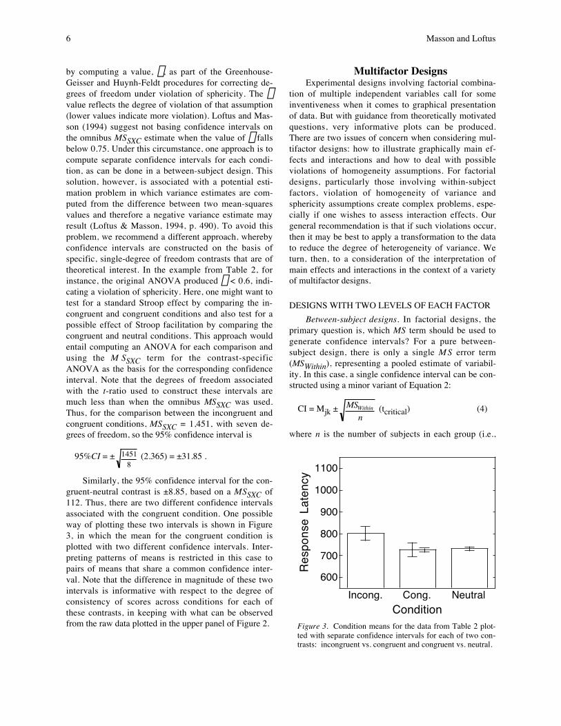
by computing a value, e, as part of the Greenhouse-Geisser and Huynh-Feldt procedures for correcting de-grees of freedom under violation of sphericity. The evalue reflects the degree of violation of that assumption(lower values indicate more violation). Loftus and Mas-son (1994) suggest not basing confidence intervals onthe omnibus MSSXC estimate when the value of e fallsbelow 0.75. Under this circumstance, one approach is tocompute separate confidence intervals for each condi-tion, as can be done in a between-subject design. Thissolution, however, is associated with a potential esti-mation problem in which variance estimates are com-puted from the difference between two mean-squaresvalues and therefore a negative variance estimate mayresult (Loftus & Masson, 1994, p. 490). To avoid thisproblem, we recommend a different approach, wherebyconfidence intervals are constructed on the basis ofspecific, single-degree of freedom contrasts that are oftheoretical interest. In the example from Table 2, forinstance, the original ANOVA produced e < 0.6, indi-cating a violation of sphericity. Here, one might want totest for a standard Stroop effect by comparing the in-congruent and congruent conditions and also test for apossible effect of Stroop facilitation by comparing thecongruent and neutral conditions. This approach wouldentail computing an ANOVA for each comparison andusing the M SSXC term for the contrast-specificANOVA as the basis for the corresponding confidenceinterval. Note that the degrees of freedom associatedwith the t-ratio used to construct these intervals aremuch less than when the omnibus MSSXC was used.Thus, for the comparison between the incongruent andcongruent conditions, MSSXC = 1,451, with seven de-grees of freedom, so the 95% confidence interval is

95%CI = ±

†

14518

(2.365) = ±31.85 .

Similarly, the 95% confidence interval for the con-gruent-neutral contrast is ±8.85, based on a MSSXC of112. Thus, there are two different confidence intervalsassociated with the congruent condition. One possibleway of plotting these two intervals is shown in Figure3, in which the mean for the congruent condition isplotted with two different confidence intervals. Inter-preting patterns of means is restricted in this case topairs of means that share a common confidence inter-val. Note that the difference in magnitude of these twointervals is informative with respect to the degree ofconsistency of scores across conditions for each ofthese contrasts, in keeping with what can be observedfrom the raw data plotted in the upper panel of Figure 2.

Multifactor DesignsExperimental designs involving factorial combina-

tion of multiple independent variables call for someinventiveness when it comes to graphical presentationof data. But with guidance from theoretically motivatedquestions, very informative plots can be produced.There are two issues of concern when considering mul-tifactor designs: how to illustrate graphically main ef-fects and interactions and how to deal with possibleviolations of homogeneity assumptions. For factorialdesigns, particularly those involving within-subjectfactors, violation of homogeneity of variance andsphericity assumptions create complex problems, espe-cially if one wishes to assess interaction effects. Ourgeneral recommendation is that if such violations occur,then it may be best to apply a transformation to the datato reduce the degree of heterogeneity of variance. Weturn, then, to a consideration of the interpretation ofmain effects and interactions in the context of a varietyof multifactor designs.

DESIGNS WITH TWO LEVELS OF EACH FACTORBetween-subject designs. In factorial designs, the

primary question is, which MS term should be used togenerate confidence intervals? For a pure between-subject design, there is only a single M S error term(MSWithin), representing a pooled estimate of variabil-ity. In this case, a single confidence interval can be con-structed using a minor variant of Equation 2:

CI = Mjk ± MSWithin

n (tcritical) (4)

where n is the number of subjects in each group (i.e.,

600

700

800

900

1000

1100


Res

pons

e La

tenc

y

ConditionFigure 3. Condition means for the data from Table 2 plot-ted with separate confidence intervals for each of two con-trasts: incongruent vs. congruent and congruent vs. neutral.


the number of observations on which each of the j x kmeans is based). This confidence interval can be plottedwith each mean and used to interpret the pattern ofmeans. If there is a serious violation of the homogeneityof variance assumption (e.g., variances differ by morethan 2:1 ratio), separate confidence intervals can beconstructed for each group in the design using Equation1.

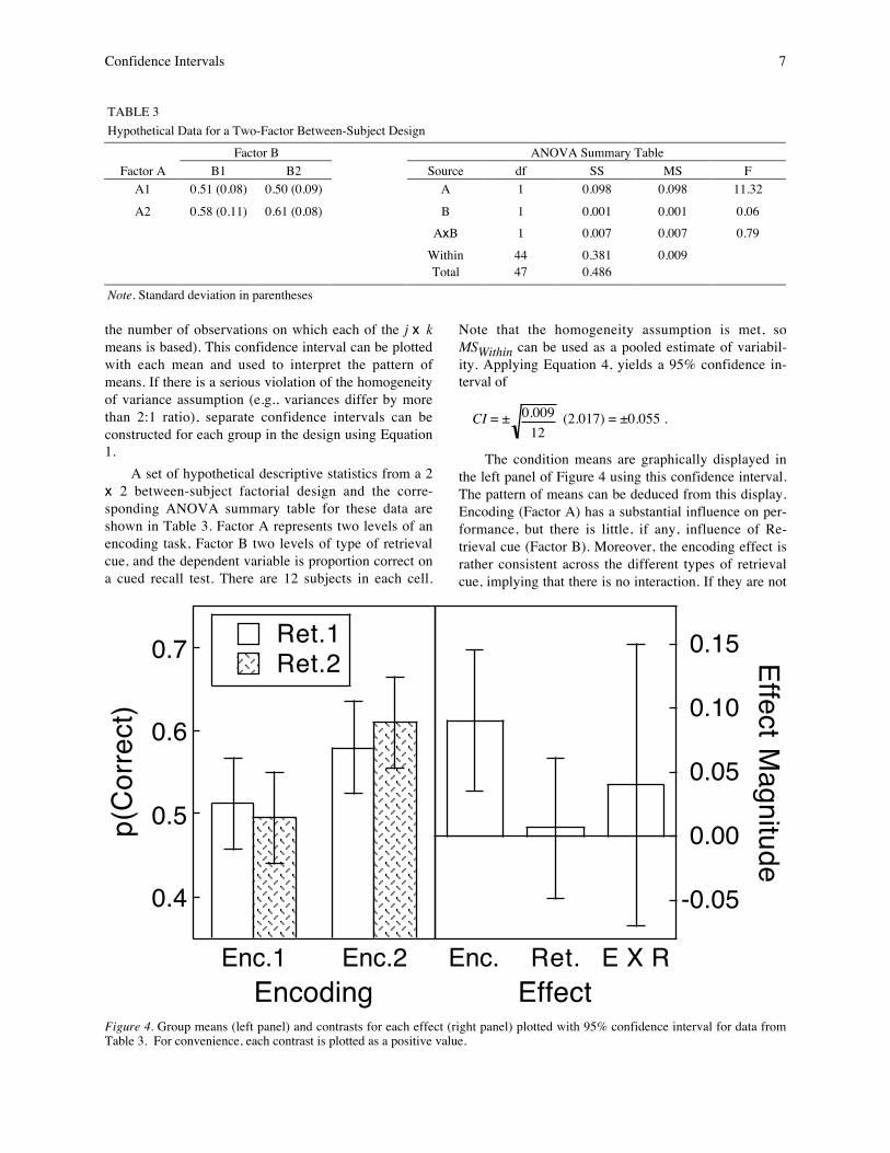
A set of hypothetical descriptive statistics from a 2x 2 between-subject factorial design and the corre-sponding ANOVA summary table for these data areshown in Table 3. Factor A represents two levels of anencoding task, Factor B two levels of type of retrievalcue, and the dependent variable is proportion correct ona cued recall test. There are 12 subjects in each cell.

Note that the homogeneity assumption is met, soMSWithin can be used as a pooled estimate of variabil-ity. Applying Equation 4, yields a 95% confidence in-terval of

CI = ± 0.00912

(2.017) = ±0.055 .

The condition means are graphically displayed inthe left panel of Figure 4 using this confidence interval.The pattern of means can be deduced from this display.Encoding (Factor A) has a substantial influence on per-formance, but there is little, if any, influence of Re-trieval cue (Factor B). Moreover, the encoding effect israther consistent across the different types of retrievalcue, implying that there is no interaction. If they are not

TABLE 3Hypothetical Data for a Two-Factor Between-Subject Design

Factor B ANOVA Summary TableFactor A B1 B2 Source df SS MS F

A1 0.51 (0.08) 0.50 (0.09) A 1 0.098 0.098 11.32

A2 0.58 (0.11) 0.61 (0.08) B 1 0.001 0.001 0.06AxB 1 0.007 0.007 0.79

Within 44 0.381 0.009Total 47 0.486

Note. Standard deviation in parentheses

0.4

0.5

0.6

0.7

Enc.1 Enc.2

Ret.1Ret.2

p(Co

rrect

)

Encoding

-0.05

0.00

0.05

0.10

0.15

Enc. Ret. E X R

Effect Magnitude

EffectFigure 4. Group means (left panel) and contrasts for each effect (right panel) plotted with 95% confidence interval for data fromTable 3. For convenience, each contrast is plotted as a positive value.

8 Masson and Loftus

very large, patterns of differences among means can bedifficult to perceive, so it may be useful to highlightselected effects.

We recommend using contrasts as the basis forcomputing specific effects and their associated confi-dence intervals. To see how this is done, recall that theconfidence intervals we have been describing so far areinterpreted as confidence intervals around single means,enabling inferences about the pattern of means. In ana-lyzing an effect defined by a contrast, we are consider-ing an effect produced by a linear combination ofmeans where that combination is defined by a set ofweights applied to the means. Contrasts may be appliedto a simple case, such as one mean versus another, withother means ignored, or to more complex cases inwhich combinations of means are compared (as whenaveraging across one factor of a factorial design to as-sess a main effect of the other factor). Applying con-trast weights to a set of means in a design results in acontrast effect (e.g., a simple difference between twomeans, a main effect, an interaction effect) and a confi-dence interval can be defined for any such effect.

In the case of our 2 x 2 example, the main effect ofEncoding (Factor A), can be defined by the followingcontrast of condition means: (A1B1 + A1B2) – (A2B1 +A2B2). The weights applied to the four condition meansthat define this contrast are: 1, 1, –1, –1. More gener-ally, the equation for defining a contrast as a linearcombination of means is

Contrast Effect = wjkMjkÂ (5)

To compute the confidence interval for a linearcombination of means, the following equation can beapplied

CIcontrast = CI wjk2Â (6)

where CI is the confidence interval from Equation 2and the wjk are the contrast weights. Notice that weightscan be of arbitrary size, as long as they meet the basicconstraint of summing to zero (e.g., 2, 2, -2, -2 wouldbe an acceptable set of weights in place of those shownabove). The size of the confidence interval for a con-trast effect will vary accordingly, as Equation 6 indi-cates. We suggest, however, that a particularly infor-mative way to define contrast weights in a manner thatreflects the averaging across means that is involved inconstructing a contrast. For example, in defining thecontrast for the Encoding main effect, we are compar-ing the average of two means against the average ofanother two means. Thus, the absolute value of the ap-propriate contrast weights that reflect this operation

would be 0.5 (summing two means and dividing by twois equivalent to multiply each mean by 0.5 and addingthe products). Thus, the set of weights that allows themain effect of the Encoding factor to be expressed as acomparison between the averages of two pairs of meanswould be 0.5, 0.5, –0.5, –0.5. Applying this set ofweights to the means from Table 3 produces

Contrast Effect = 0.5(0.51) + 0.5(0.50) + (–0.5)(0.58)+ (–0.5)(0.61) = –0.0905.

The mean difference between the two encodingconditions, then, is slightly more than 0.09. The confi-dence interval for this contrast is equal to the originalconfidence interval for individual means because thesum of the squared weights equals 1, so the second termin Equation 6 equals 1. This Encoding main effect con-trast, representing the main effect of Encoding (FactorA), and its confidence interval are plotted in the rightpanel of Figure 4. For convenience we have plotted thecontrast effect as a positive value. This move is notproblematic because the sign of the effect is arbitrary(i.e., it is determined by which level of Factor A wehappened to call level 1 and which we called level 2).Note that the confidence interval does not include zero,supporting the conclusion that the Encoding task ma-nipulation favors condition A2, as implied by the pat-tern of means in the left panel of Figure 4.

For the main effect of Retrieval cue, the weightswould be 0.5, –0.5, 0.5, –0.5. The absolute values ofthese weights are again 0.5 because the same type ofcomparison is being made as in the case of the Encod-ing main effect (comparison between averages of pairsof means). The contrast effect for the Retrieval cue ef-fect and its confidence interval (which is the same asfor the Encoding task effect because the contrastweights were identical) is shown in the right panel ofFigure 4. The confidence interval includes zero, indi-cating that type of retrieval cue made little or no differ-ence to recall performance.

For the interaction, however, we have a somewhatdifferent situation. The interaction is a difference be-tween differences, rather than a difference betweenaverages. That is, a 2 x 2 interaction is based on com-puting the difference between the effect of Factor A atone level of Factor B, and the effect of A at the otherlevel of B. In the present example, this contrast wouldbe captured by the weights 1, –1, –1, 1. (This same setof weights can also be interpreted as representing thedifference between the effect of Factor B at one level ofFactor A and the effect of B at the other level of A.)Applying these weights for the interaction yields thefollowing contrast effect:

Contrast Effect = 1(0.51) + (–1)(0.50) + (–1)(0.58)


+ 1(0.61) = 0.04 .Now consider the confidence interval for this ef-

fect. The square root of the sum of these squaredweights is 2, so applying Equation 6 to obtain the con-fidence interval for the effect, we have

CIcontrast = ±0.055(2) = ±0.110 .

The interaction effect and its confidence intervalare plotted in the right panel of Figure 4. Note that thisconfidence interval is twice the size of the confidenceinterval for the main effects. This occurs because weare computing a difference between differences, ratherthan between averages. Even so, this is a somewhatarbitrary stance. We could just as easily have convertedthe weights for the interaction contrast to ±0.5 andwound up with a confidence interval equal to that forthe two main effects. But in treating the interactioncontrast as a difference between differences and using±1 as the weights, the resulting numerical contrast ef-fect more directly reflects the concept underlying thecontrast.

The principles described here easily can be scaledup to accommodate more than 2 factors. In such cases itwould be particularly useful to plot each of the maineffects and interactions as contrasts, as shown in Figure4, because magnitude of interactions beyond two fac-tors can be very hard to visualize based on a display ofindividual means. Moreover, main effects in such de-signs involve collapsing across three or more means,again making it difficult to assess such effects. At thesame time, a major advantage of plotting individualmeans with confidence intervals is that one can exam-ine patterns of means that may be more specific thanstandard main effects and interactions. And, of course,the plot of individual means, or means collapsed acrossone of the factors, can reveal the pattern of interaction

effects (e.g., a cross-over interaction).Within-subject designs. In a within-subject design,

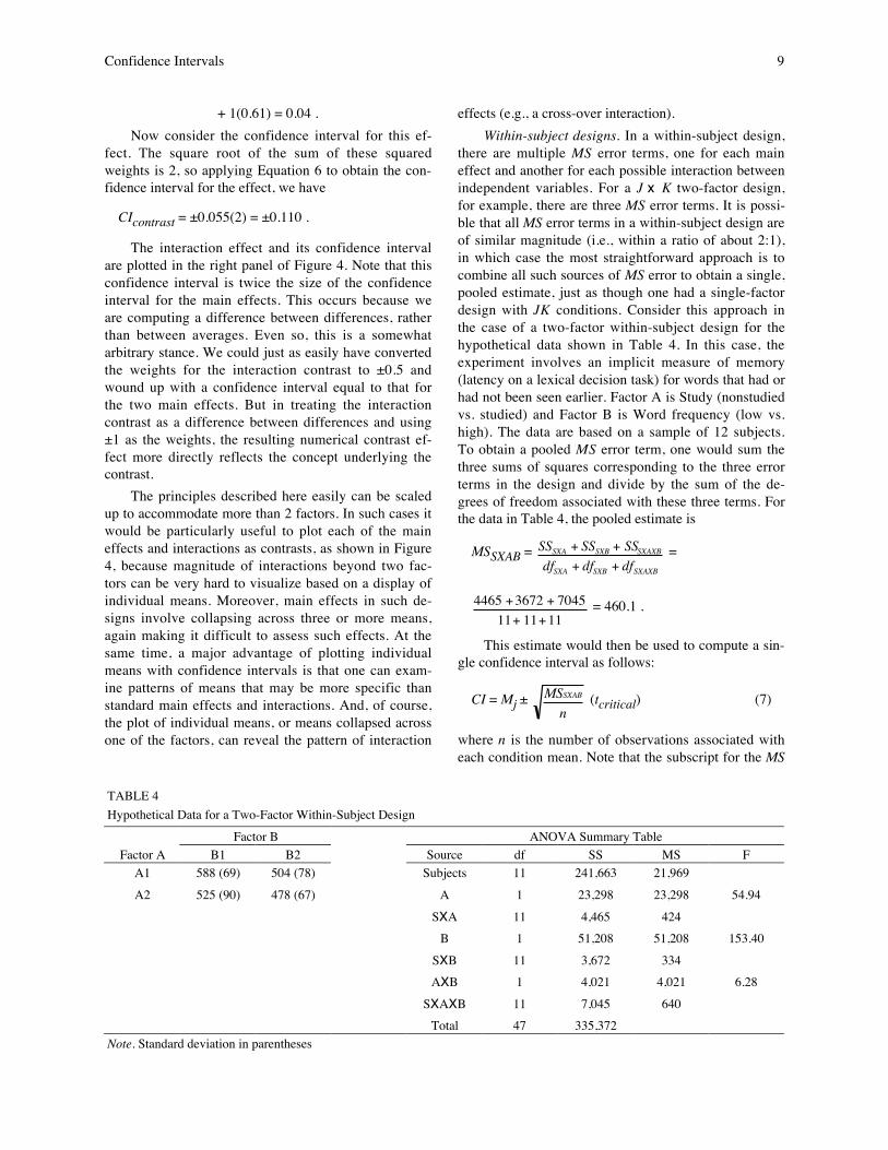
there are multiple MS error terms, one for each maineffect and another for each possible interaction betweenindependent variables. For a J x K two-factor design,for example, there are three MS error terms. It is possi-ble that all MS error terms in a within-subject design areof similar magnitude (i.e., within a ratio of about 2:1),in which case the most straightforward approach is tocombine all such sources of MS error to obtain a single,pooled estimate, just as though one had a single-factordesign with JK conditions. Consider this approach inthe case of a two-factor within-subject design for thehypothetical data shown in Table 4. In this case, theexperiment involves an implicit measure of memory(latency on a lexical decision task) for words that had orhad not been seen earlier. Factor A is Study (nonstudiedvs. studied) and Factor B is Word frequency (low vs.high). The data are based on a sample of 12 subjects.To obtain a pooled MS error term, one would sum thethree sums of squares corresponding to the three errorterms in the design and divide by the sum of the de-grees of freedom associated with these three terms. Forthe data in Table 4, the pooled estimate is

MSSXAB = SSSXA + SSSXB + SSSXAXB

dfSXA + dfSXB + dfSXAXB

=

4465 +3672 + 704511+ 11+11

= 460.1 .

This estimate would then be used to compute a sin-gle confidence interval as follows:

CI = Mj ± MSSXAB

n (tcritical) (7)

where n is the number of observations associated witheach condition mean. Note that the subscript for the MS

TABLE 4Hypothetical Data for a Two-Factor Within-Subject Design


A1 588 (69) 504 (78) Subjects 11 241,663 21,969A2 525 (90) 478 (67) A 1 23,298 23,298 54.94

SXA 11 4,465 424B 1 51,208 51,208 153.40

SXB 11 3,672 334AXB 1 4,021 4,021 6.28

SXAXB 11 7,045 640Total 47 335,372


10 Masson and Loftus

term in this equation reflects a pooled estimate of MSerror, not the MS error term for the interaction alone.Thus, the degrees of freedom for the critical t-ratiowould be the sum of the degrees of freedom for thethree MS error terms. For the data in Table 4, the 95%confidence interval would be

CI = ± 460.112

(2.036) = ±12.61 .

This confidence interval can be plotted with eachmean in the design and used to interpret patterns amongany combination of means. The left panel of Figure 5presents the data from Table 4 in this manner. Onecould also display each of the main effects and the in-teraction as contrasts as was done for the previous be-tween-subjects example in Figure 4. But another alter-native would be to highlight the interaction by plottingit as means of difference scores computed for each levelof one factor. In the present example, it is of theoreticalinterest to consider the effect of prior study at each ofthe two frequency levels. For each subject, then, onecould compute the effect of prior study at each level ofword frequency, producing two scores per subject. Themeans of these difference scores are shown in the rightpanel of Figure 5. The confidence interval for this inter-action plot can be computed from a MS error term ob-

tained by computing a new ANOVA with only Factor Bas a factor and using difference scores on Factor A (i.e.,A1 – A2) for each subject, with one such score com-puted at each level of B. The resulting MS error term is1,281. The confidence interval for this interaction effectusing Equation 3 and a critical t-ratio for 11 degrees offreedom is

CI = ± 128112

(2.201) = ± 22.74

Next, consider how to plot the means and confi-dence intervals when it is not advisable to pool the threeMS error terms in a two-factor within-subject design.One could combine a pair of terms if they are suffi-ciently similar (within a factor of about two) and com-pute a confidence interval from a pooled MS errorbased on those two sources. A separate confidence in-terval could be computed for the other effect whose MSerror is very different from the other two. The latterconfidence interval would be appropriate for drawingconclusions only about the specific effect with which itis associated. To illustrate how this might be done, letus assume that in Table 4 the M SSXAXB term wasdeemed much larger than the other two error terms, soonly the MSSXA and MSSXB are pooled and the result-ing confidence interval is plotted with the four means of

450

500

550

600

Low High

NewOld

Res

pons

e La

tenc

y

Word Frequency

0

25

50

75

100

Low High

Study Effect

Figure 5. Condition means and interaction plot with 95% within-subject confidence interval for data from Table 4.


the design. A subsidiary plot, like that shown in theright panel of either Figure 4 (to display all three effectsin the design) or Figure 5 (to display just the interac-tion) could then be constructed specifically for the in-teraction using a confidence interval computed fromMSSXAXB.

As an additional example of a case in which not all

MS error terms are similar, consider the data set in Ta-ble 5. These data are the descriptive statistics andANOVA for a 2 x 2 within-subject design with 16 sub-jects. Here, we have a case in which a word stem com-pletion test is used as an implicit measure of memoryand the factors are Study (Factor A), referring towhether or not a stem's target completion had been

TABLE 5Hypothetical Data for a Two-Factor Within-Subject Design


A1 .33 (.09) .23 (.11) Subjects 15 0.211 0.014

A2 .18 (.07) .20 (.09) A 1 0.126 0.126 23.12SXA 15 0.082 0.005

B 1 0.023 0.023 2.13SXB 15 0.16 0.011AXB 1 0.052 0.052 13.27

SXAXB 15 0.059 0.004Total 63 0.713


0.15

0.20

0.25

0.30

0.35

Immed. Delay

StudiedNonstudied

p(Ta

rget

Com

plet

ion)

Delay IntervalStd. Del. SxD

Effect

Delay: ±0.056

0.00

0.05

0.10

0.15

0.20 Effect Magnitude

Figure 6. Condition means (left panel) and contrasts for each effect (right panel) plotted with 95% confidence interval for datafrom Table 5. For convenience, each contrast is plotted as a positive value.


studied previously, and Delay interval (Factor B) be-tween the study and test phase (i.e., the test followsimmediately or after a delay). In this case, M SSXB isquite dissimilar from the other two error terms, so wemight wish to plot a confidence interval based onpooling MSSXA and MSSXAXB, to be plotted with eachmean, then construct a separate confidence intervalbased on MSSXB for use in the interpretation of FactorB. The confidence interval obtained by pooling acrossMSSXA and MSSXAXB is found by pooling the MS errorterms

MSSxC = 0.082 + 0.05915 +15

= 0.0047 ,

then computing the confidence interval using a t-ratio with dfSXA + dfSXAXB = 15 + 15 = 30 degrees offreedom:

CI = ± 0.004716

(2.042) = ±0.035 .

The confidence interval for the main effect of B isbased on a t-ratio with dfSXB = 15 degrees of freedom:

CI = ± 0.01116

(2.132) = ±0.056 .

This latter confidence interval could be strategi-cally placed so that it is centered at a height equal to thegrand mean, as shown in the left panel of Figure 6. Thisdisplay gives an immediate impression of the magni-tude of the B main effect. In addition, the right panel ofFigure 6 shows all three effects of this design with theappropriate confidence interval for each. The contrastweights for each effect were the same as in the be-tween-subject design above. Thus, the confidence inter-vals for the A main effect and for the interaction effectare different, despite being based on the same MS errorterm. The extension of these methods to designs withmore than two factors, each having two levels, could

proceed as described for the case of between-subjectdesigns.

Mixed designs. In a mixed design, there is at leastone between-subject and at least one within-subjectfactor. We will consider in detail this minimal case,although our analysis can be extended to cases involv-ing a larger number of factors. In the 2-factor case,there are two different MS error terms. One is the MSwithin groups and is used to test the between-subjectfactor's main effect; the other is the MS for the interac-tion between the within-subject factor and subjects (i.e.,the consistency of the within-subject factor across sub-jects) and is used to test the within-subject factor's maineffect and the interaction between the between-subjectand the within-subject factors. Unlike two-factor de-signs in which both factors are between- or both arewithin-subject factors, it would be inappropriate to poolthe two MS error terms in a mixed design. Rather, sepa-rate confidence intervals must be constructed becausethe variability reflected in these two MS error terms areof qualitatively different types––one reflects variabilitybetween subjects and the other represents variability ofthe pattern of condition scores across subjects. The con-fidence interval based on the within-subject MS errorterm (MSSxC) is computed using Equation 3, and theconfidence interval for the MS error term for the be-tween-subject factor (M SWithin) is computed usingEquation 2.

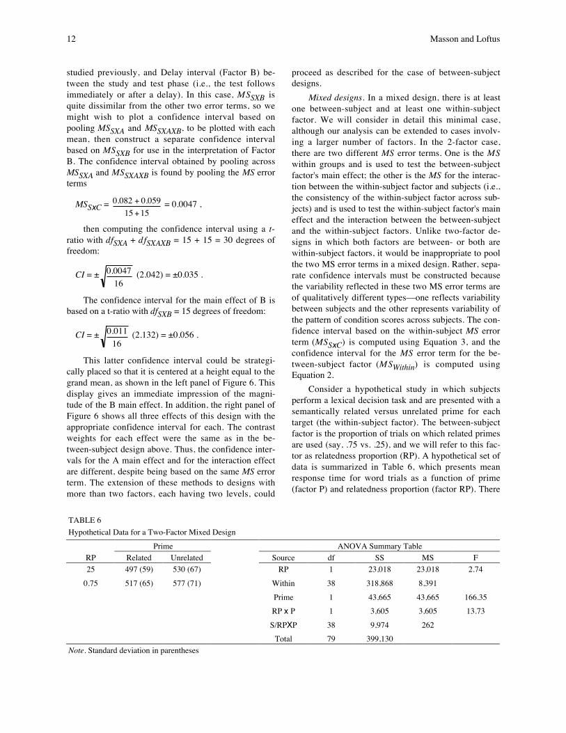
Consider a hypothetical study in which subjectsperform a lexical decision task and are presented with asemantically related versus unrelated prime for eachtarget (the within-subject factor). The between-subjectfactor is the proportion of trials on which related primesare used (say, .75 vs. .25), and we will refer to this fac-tor as relatedness proportion (RP). A hypothetical set ofdata is summarized in Table 6, which presents meanresponse time for word trials as a function of prime(factor P) and relatedness proportion (factor RP). There

TABLE 6Hypothetical Data for a Two-Factor Mixed Design

Prime ANOVA Summary TableRP Related Unrelated Source df SS MS F25 497 (59) 530 (67) RP 1 23,018 23,018 2.74

0.75 517 (65) 577 (71) Within 38 318,868 8,391Prime 1 43,665 43,665 166.35RP x P 1 3,605 3,605 13.73S/RPXP 38 9,974 262

Total 79 399,130Note. Standard deviation in parentheses


are 20 subjects in each RP condition. The table alsoshows the results of a mixed-factor ANOVA applied tothese data. In this case, the prime main effect and theinteraction are clearly significant. Notice also that thetwo MS error terms in this design are, as will usually bethe case, very different, with the MSWithin term muchlarger than the MS error for the within-subject factorand the interaction. The corresponding confidence in-tervals, then, are also very different. For the main effectof the between-subject factor, RP, the confidence inter-val (based on the number of observations contributingto each mean; two scores per subject in this case), usingEquation 2, is

CI = ± 8, 391(2)20

(2.025) = 29.33 .

The confidence interval for the within-subject fac-tor, P, and the interaction, using Equation 3, is

CI = ± 26220

(2.025) = 7.33 .

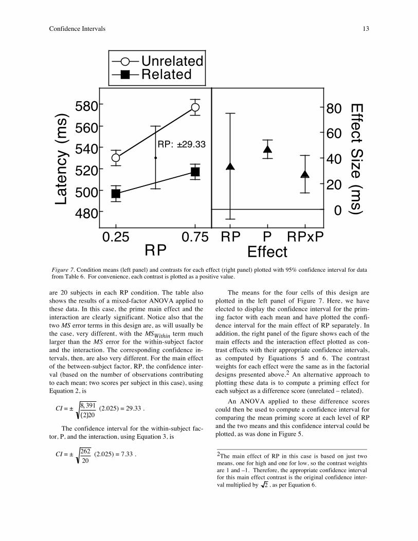
The means for the four cells of this design areplotted in the left panel of Figure 7. Here, we haveelected to display the confidence interval for the prim-ing factor with each mean and have plotted the confi-dence interval for the main effect of RP separately. Inaddition, the right panel of the figure shows each of themain effects and the interaction effect plotted as con-trast effects with their appropriate confidence intervals,as computed by Equations 5 and 6. The contrastweights for each effect were the same as in the factorialdesigns presented above.2 An alternative approach toplotting these data is to compute a priming effect foreach subject as a difference score (unrelated – related).

An ANOVA applied to these difference scorescould then be used to compute a confidence interval forcomparing the mean priming score at each level of RPand the two means and this confidence interval could beplotted, as was done in Figure 5.

UnrelatedRelated

RP: ±29.33

480500520540560580

0.25 0.75

Late

ncy

(ms)

RP

020406080

RP P RPxP

Effect Size (ms)

EffectFigure 7. Condition means (left panel) and contrasts for each effect (right panel) plotted with 95% confidence interval for datafrom Table 6. For convenience, each contrast is plotted as a positive value.

2The main effect of RP in this case is based on just twomeans, one for high and one for low, so the contrast weightsare 1 and –1. Therefore, the appropriate confidence intervalfor this main effect contrast is the original confidence inter-val multiplied by 2 , as per Equation 6.


DESIGNS WITH THREE OR MORE LEVELS OF AFACTOR

The techniques described above can be generalizedto designs in which at least one of the factors has morethan two levels. In general, the first step is to plotmeans with confidence intervals based on a pooled MSerror estimate where possible (in a pure within-subjectdesign with MS error terms of similar size) or a MSerror term that emphasizes a theoretically motivatedcomparison. In addition, one can plot main effects andinteractions as illustrated in the previous section. Withthree or more levels of one factor, however, there is anadditional complication: For any main effect or interac-tion involving a factor with more than two levels, morethan one contrast can be computed. This fact does notmean that one necessarily should compute and report asmany contrasts as degrees of freedom allow. Indeed,there may be only one theoretically interesting contrast.The important point to note here is simply that one hasthe choice of defining and reporting those contrasts thatare of theoretical interest. Moreover, in designs withone within-subject factor that has two levels, an inter-action plot can be generated by computing differencescores based on that factor (e.g., for each subject, sub-tract the score on level 1 of that factor from the score onlevel 2), as described above. The mean of these differ-ence scores for each level of the other factor(s) can thenbe plotted, as in Figure 5.

Let us illustrate, though, an approach in whichcontrast effects are plotted in addition to individualcondition means. For this example, consider a 2 x 3within-subject design used by a researcher to investi-gate conscious and unconscious influences of memoryin the context of Jacoby's (1991) process-dissociationprocedure. In a study phase, subjects encode one set ofwords in a semantic encoding task and another set in a

nonsemantic encoding task. In the test phase, subjectsare given a word stem completion task with three setsof stems. One set can be completed with semanticallyencoded words from the study list, another set can becompleted with nonsemantically encoded words, andthe final set is used for a group of nonstudied words.For half of the stems of each type, subjects attempt torecall a word from the study list and to use that item asa completion for the stem (inclusion instruction). Forthe other half of the stems, subjects are to provide acompletion that is not from the study list (exclusioninstructions). The factors, then, are encoding (semantic,nonsemantic, nonstudied) and test (inclusion, exclu-sion).

A hypothetical data set from 24 subjects is shownin Table 7, representing mean proportion of stems forwhich target completions were given. The three MSerror terms in the accompanying ANOVA summarytable are similar to one another, so a combined MS errorterm can be used to compute a single confidence inter-val for the plot of condition means. The combined MSerror is

MSSxC = 0.615 + 1.084 + 0.67523 + 46 + 46

= 0.021 .

Based on M SSxC, the confidence interval associ-ated with each mean in this study is

CI = ± 0.02124

(1.982) = ± 0.042 .

The means from Table 7 are plotted in the leftpanel of Figure 8 with this confidence interval.

A number of inferences can be drawn from thispattern of means (e.g., semantic encoding producesmore stem completion than nonsemantic encoding un-der inclusion instructions, but the reverse occurs under

TABLE 7Hypothetical Data for a Two-Factor Within-Subject Design with Three Levels of One Factor

Encoding Tasl ANOVA Summary TableInstr Sem Nonseman New Source df SS MS FIncl. .66 (.11) .51 (.16) .30 (.11) Subjects 23 0.635 0.028Excl. .32 (.16) .47 (.20) .28 (.14) Instr. 1 0.618 0.618 23.13

S x Instr. 23 0.615 0.027Encoding 2 1.278 0.639 27.13S x Enc. 46 1.084 0.024

I x E 2 0.802 0.401 27.32S x I x E 46 0.675 0.015

Total 143 5.707Note. Standard deviation in parentheses


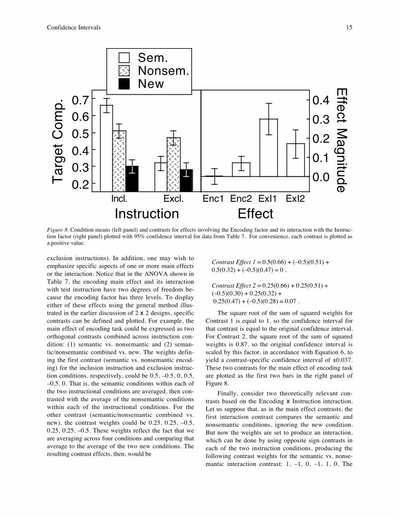
exclusion instructions). In addition, one may wish toemphasize specific aspects of one or more main effectsor the interaction. Notice that in the ANOVA shown inTable 7, the encoding main effect and its interactionwith test instruction have two degrees of freedom be-cause the encoding factor has three levels. To displayeither of these effects using the general method illus-trated in the earlier discussion of 2 x 2 designs, specificcontrasts can be defined and plotted. For example, themain effect of encoding task could be expressed as twoorthogonal contrasts combined across instruction con-dition: (1) semantic vs. nonsemantic and (2) seman-tic/nonsemantic combined vs. new. The weights defin-ing the first contrast (semantic vs. nonsemantic encod-ing) for the inclusion instruction and exclusion instruc-tion conditions, respectively, could be 0.5, –0.5, 0, 0.5,–0.5, 0. That is, the semantic conditions within each ofthe two instructional conditions are averaged, then con-trasted with the average of the nonsemantic conditionswithin each of the instructional conditions. For theother contrast (semantic/nonsemantic combined vs.new), the contrast weights could be 0.25, 0.25, –0.5,0.25, 0.25, –0.5. These weights reflect the fact that weare averaging across four conditions and comparing thataverage to the average of the two new conditions. Theresulting contrast effects, then, would be

Contrast Effect 1 = 0.5(0.66) + (–0.5)(0.51) +0.5(0.32) + (–0.5)(0.47) = 0 ,

Contrast Effect 2 = 0.25(0.66) + 0.25(0.51) +(–0.5)(0.30) + 0.25(0.32) + 0.25(0.47) + (–0.5)(0.28) = 0.07 .

The square root of the sum of squared weights forContrast 1 is equal to 1, so the confidence interval forthat contrast is equal to the original confidence interval.For Contrast 2, the square root of the sum of squaredweights is 0.87, so the original confidence interval isscaled by this factor, in accordance with Equation 6, toyield a contrast-specific confidence interval of ±0.037.These two contrasts for the main effect of encoding taskare plotted as the first two bars in the right panel ofFigure 8.

Finally, consider two theoretically relevant con-trasts based on the Encoding x Instruction interaction.Let us suppose that, as in the main effect contrasts, thefirst interaction contrast compares the semantic andnonsemantic conditions, ignoring the new condition.But now the weights are set to produce an interaction,which can be done by using opposite sign contrasts ineach of the two instruction conditions, producing thefollowing contrast weights for the semantic vs. nonse-mantic interaction contrast: 1, –1, 0, –1, 1, 0. The

0.20.30.40.50.60.7

Incl. Excl.

Sem.Nonsem.New

Targ

et C

omp.

Instruction

0.00.10.20.30.4

Enc1 Enc2 ExI1 ExI2

Effect Magnitude

EffectFigure 8. Condition means (left panel) and contrasts for effects involving the Encoding factor and its interaction with the Instruc-tion factor (right panel) plotted with 95% confidence interval for data from Table 7. For convenience, each contrast is plotted asa positive value.


weights reflect the intended expression of the interac-tion effect as a difference between difference scores.This contrast effect is

Contrast Effect 3 = 1(0.66) + (–1)(0.51) + (–1)(0.32)+ 1(0.47) = 0.30 .

The square root of the sum of the squared contrastweights in this case is 2, so the corresponding confi-dence interval is (±0.042)(2) = ±0.084. Let us furtherassume that the other contrast for the interaction effectwill also parallel the second main effect contrast, inwhich the average of the semantic and nonsemanticconditions is compared to the new condition, but againusing opposite signs for the two instruction conditions:0.5, 0.5, –1, –0.5, –0.5, 1. Applying these weights to themeans produces the following contrast:

Contrast Effect 4 = 0.5(0.66) + 0.5(0.51) + (–1)(0.30)+ (–0.5)(0.32) + (–0.5)(0.47) + 1(0.28) = 0.17 .

The confidence interval for this interaction is(±0.042)(1.73) = ±0.073. The two interaction contrastsare plotted as the final two bars in the right panel ofFigure 8.

There are, of course, other possible contrasts thatcould have been defined and plotted. Loftus (2002)presented further examples of contrast effects that canbe used to make full use of graphical displays of datafrom factorial designs.

PowerOne particularly important advantage of graphical

presentation of data, and especially confidence inter-vals, is that such presentations provide informationconcerning statistical power. The power of an experi-ment to detect some effect becomes very importantwhen the effect fails to materialize and that failure car-ries substantial theoretical weight. The prescription forcomputing power estimates under the standard NHSTapproach requires that one specify a hypothetical effectmagnitude. Although it is possible to select such a valueon the basis of theoretical expectation or related empiri-cal findings, the estimate of power depends to a largedegree on this usually arbitrary value. An alternativeapproach is to report not just a single power estimatebased on a single hypothesized effect magnitude, but apower curve that presents power associated with a widerange of possible effect magnitudes. In practice, this israrely (if ever) done.

With graphical plots of data, however, we have aready-made alternative means of displaying the powerof an experiment. Specifically, the smaller the confi-

dence intervals, the greater the amount of statisticalpower and, more important, the greater the confidencewe can place in the observed pattern of means. To il-lustrate this concept, consider two different data setsfrom a reaction time task, each representing a one-factor within-subject design with two levels of the fac-tor. The means and the MSSxC in the two data sets arethe same, but the sample size is much larger in the sec-ond case leading to a smaller confidence interval for themeans. The means and confidence intervals are shownin Figure 9. The floating confidence interval in eachcase is the 95% confidence interval for the differencebetween means, computed using Equation 6 and thecontrast weights 1 and –1. It is immediately obviousthat we can have greater confidence in the pattern ofmeans in the set of data on the right side of Figure 9.

In normal situations, only one of these two sets ofdata would be available, so how can one know whetherthe confidence interval, either for means or for differ-ences between means is small enough to indicate thatsubstantial statistical power is available? There are anumber of benchmarks one might rely on. For example,for commonly used tasks there often are well estab-lished rules of thumb regarding how small an effect canbe detected (e.g., in lexical decision tasks, reliable ef-fects are usually 20 ms or more). Alternatively, as inpower estimation under NHST, there may be empiricalor theoretical reasons to expect an effect of a particularmagnitude. If an expected effect size is larger than theobserved effect and larger than the confidence interval

450

500

550

600

A B

Late

ncy

(ms)

ConditionA B

Mean diff. CI = ±56.6

Mean diff. CI = ±17.0

Figure 9. Condition means for hypothetical data representingan experiment with low power (left panel) and an experimentwith high power (right panel), plotted with 95% within-subject confidence intervals. The floating confidence intervalrepresents the 95% confidence interval for the differencebetween means.


for the difference between means, it is reasonable toconclude that the true effect is smaller than what wasexpected.

Another kind of benchmark for evaluating powercomes from inherent limits on scores in a particularexperiment. For instance, consider an experiment onlong-term priming. If one is assessing differences inpriming between two study conditions, it is possible tosee immediately whether the study has adequate powerto detect a difference in priming, because adequatepower depends on whether the confidence interval forthe difference between means is smaller or larger thanthe observed priming effects. If the confidence intervalfor the difference between means is larger than thepriming effects themselves, then clearly there is notadequate power––one condition would have to have anegative priming effect for a difference to be found!

ConclusionWe have described a number of approaches to

graphical presentation of data in the context of classicalfactorial designs that typify published studies in ex-perimental psychology. Our emphasis has been on theuse of confidence intervals in conjunction with graphi-cal presentation to allow readers to form inferencesabout the patterns of means (or whatever statistic theauthor opts to present). We have also tried to conveythe notion that authors have a number of options avail-able with respect to construction of graphical presenta-tions of data and that selection among these options canbe guided by specific questions or hypotheses abouthow manipulated factors are likely to influence behav-ior. The approach we have described represents a sup-plement or, for the bold among us, an alternative tostandard NHST methods.

ReferencesChow, S. L. (1998). The null-hypothesis significance-

test procedure is still warranted. Behavioral andBrain Sciences, 21, 228-238.

Cohen, J. (1990). Things I have learned (so far). Ameri-can Psychologist, 45, 1304-1312.

Cohen, J. (1994). The earth is round (p < .05). Ameri-can Psychologist, 49, 997-1003.

Estes, W. K. (1997). On the communication of infor-mation by displays of standard errors and confi-dence intervals. Psychonomic Bulletin & Review,4, 330-341.

Goldstein, H., & Healy, M. J. R. (1995). The graphicalpresentation of a collection of means. Journal ofthe Royal Statistical Society, Series A, 158, 175-177.

Hagen, R. L. (1997). In praise of the null hypothesisstatistical test. American Psychologist, 52, 15-24.

Hunter, J. E. (1997). Needed: A ban on the significancetest. Psychological Science, 8, 3-7.

Jacoby, L. L. (1991). A process dissociation frame-work: Separating automatic from intentional usesof memory. Journal of Memory and Language,30, 513-541.

Krueger, J. (2001). Null hypothesis significance testing:On the survival of a flawed method. AmericanPsychologist, 56, 16-26.

Lewandowsky, S., & Maybery, M. (1998). The criticsrebutted: A Pyrrhic victory. Behavioral andBrain Sciences, 21, 210-211.

Loftus, G. R. (1991). On the tyranny of hypothesistesting in the social sciences. ContemporaryPsychology, 36, 102-105.

Loftus, G.R. (1993). A picture is worth a thousand p-values: On the irrelevance of hypothesis testingin the computer age. Behavior Research Meth-ods, Instrumentation & Computers, 25, 250-256.

Loftus, G.R. (1996). Psychology will be a much betterscience when we change the way we analyzedata. Current Directions in Psychological Sci-ence, 5, 161-171.

Loftus, G. R. (2002). Analysis, interpretation, and vis-ual presentation of experimental data. In H.Pashler (Ed.), Stevens' handbook of experimentalpsychology (Vol. 4, pp. 339-390). New York:John Wiley and Sons.

Loftus, G. R. & Masson, M. E. J. (1994). Using confi-dence intervals in within-subject designs. Psy-chonomic Bulletin & Review, 1, 476-490.

Schmidt, F. (1996). Statistical significance testing andcumulative knowledge in Psychology: Implica-tions for training of researchers. PsychologicalMethods, 1, 115-129.

Tryon, W. W. (2001). Evaluating statistical difference,equivalence, and indeterminacy using inferentialconfidence intervals: An integrated alternativemethod of conducting null hypothesis statisticaltests. Psychological Methods, 6, 371-386.

Tufte, E. R. (1983). The visual display of quantitativeinformation. Cheshire, CT: Graphics Press.

Documents

Using Confidence Intervals for Graphically Based Data Interpretation