Using Color

to Understand

Light Transmission By G.v. Grigoryan, I.T. Lima, Jr., T. Yu, V.S. Grigoryan and C.R. Menyuk

Historically, physicists and engineers have always portrayed wave transmission using line diagrams in which the amplitude is shown as a function of time and distance. This sort of drawing tells us what is happening to the wave amplitude. However, waves are characterized by their phase as well as their amplitude, and these drawings tell us nothing about the phase evolution. The advent of modern computers with col­or monitors and inexpensive color printers allows us to solve this problem in a visu­ally appealing way by using a periodic color map to portray phase information. We can also portray information about the local frequency, the phase derivative with respect to time, using an aperiodic color map. We apply this approach to study light propagation in optical fibers.

44 Optics & Photonics News/August 2000 1047-6938/00/08/0044/08-$0015.00 © Optical Society of America

From the earliest days of scientific discovery, scientists have used illustrations to under­stand and explain natural phenomena. How­ever, even though we see and think in color, most illustrations in textbooks and scientific publications are simple black-and-white line drawings. Historically, the high cost of pre­

senting images in color has been a barrier to using color to present scientific results. However, the advent of rela­tively inexpensive color monitors and color printers has led to a dramatic change in the last decade. Color presen­tations are now quite common in scientific meetings, and it is our view that scientific journals and textbooks cannot be far behind. The publication by the Optical Society of America of Optics Express—an entirely on-line journal that allows the easy incorporation of multimedia images and color—is an important step in this direction. While the technology now exists to make greater use of color, our concepts of how to use color have not really kept pace. For the most part, we still use simple line drawings, employing changes in color in the same way we previous­ly used a change in the line—from straight to dashed to dotted—to indicate a change in the parameters.

The use of line drawings is particularly ineffective when discussing wave propagation. A wave is characterized by both its amplitude, or its intensity, and its phase. Phase varies periodically, so it is hard to represent it well using line diagrams. Moreover, one would ideally like to present the amplitude and phase information simultaneously, since both are important. Here, we will describe an approach in which we use a periodic color map to represent phase while the height of the colored bar represents the intensity at each point in time. We will use a similar approach to represent the local frequency, which is just the time derivative of the phase. In contrast to the phase, which varies between - Π and Π , the local frequency can have any value; for this rea­son, it is most appropriate to use an aperiodic color map.

We will apply this approach to studying simple exam­ples from optical fiber transmission systems. The practical importance of these systems is well known. Data transmis­sion rates have increased by four orders of magnitude in the last decade, largely powered by improvements in optical transmission technology.1 This immense increase in data rates has in turn led to the rapid growth of the Internet and the World Wide Web, creating new paradigms for global communications.2,3 It is less well known but equally true that optical fibers present us with a remarkable opportunity for studying nonlinear wave phenomena. Under some cir­cumstances, light transmission in an optical fiber is described by the nonlinear Schrödinger equation4

where U(z,t) = A(z,t)exp[iφ(z,t)] is the complex wave envelope, while A(z,t) is its amplitude and φ(z,t) is its phase. In Equation 1, the variable z is distance along the fiber and t is the retarded time defined as t = τ - z/V g, where Τ is the physical time and Vg is the group velocity.

The quantity β"(z) is the dispersion. The nonlinear coef­ficient γ equals n 2 ω 0 /A e f f c, where n 2 is the Kerr coeffi­cient, ω0 is the central radial frequency of the wave, A e f f

is the effective area of the core, and c is the speed of light. In modern-day communications systems, the dispersion β"(z) often varies periodically, but when it is constant, Equation 1 falls into that special class of nonlinear equa­tions that mathematicians refer to as "integrable." It can be solved using the inverse scattering method, and it has soliton solutions. It also has a rich set of other solutions, particularly when we allow β"(z) to vary.

In the remainder of this paper, using a set of increasing­ly complex examples, we will apply our approach for rep­resenting intensity along with the phase or local frequency. We will begin by neglecting the nonlinearity, setting γ = 0. In this case, our system is purely dispersive. We next neglect the dispersion, setting β"(z) = 0, and observe non­linearly induced self-phase modulation.5 - 7 In both these cases, there is a simple analytical expression for the solu­tion in the frequency domain and the time domain, respectively. We then consider a case with both non-zero disper­sion and non-zero non-linearity, in which an initial pulse breaks up into a soliton and a dis­persive background. 8 , 9

Finally, we consider an example in which β"(z) varies periodically so that dispersion-man­aged solitons can propa­gate. These periodically stationary pulses have been the subject of intensive study in recent years 1 0 , 1 1 and may be of use in communication systems.

Linear dispersive waves If we neglect the nonlinear term in Equation 1, it becomes simply

which is the linear dispersive wave equation. This equa­tion applies to optical fiber transmission when the pulse power is low and the distances are short. In this case, the refractive index of the medium is not affected by the optical pulse. Equation 2 can be solved using Fourier transform methods, as shown in Figure 1. The equation governing the Fourier transform of U(z,t), which we will write as Ũ(z,ω), is

Figure 1. Illustration of the procedure for calculat­ing the evolution of linear, dispersive waves. Rather than directly calculating the behavior in the time domain, as shown by the dashed line, it is more efficient to find the initial Fourier transform. From the initial Fourier transform, the next step is to determine the evolution at any z using Equation 4 . Finally, one determines the evolution in the time domain by taking the inverse Fourier transform.

Optics & Photonics News/August 2000 45

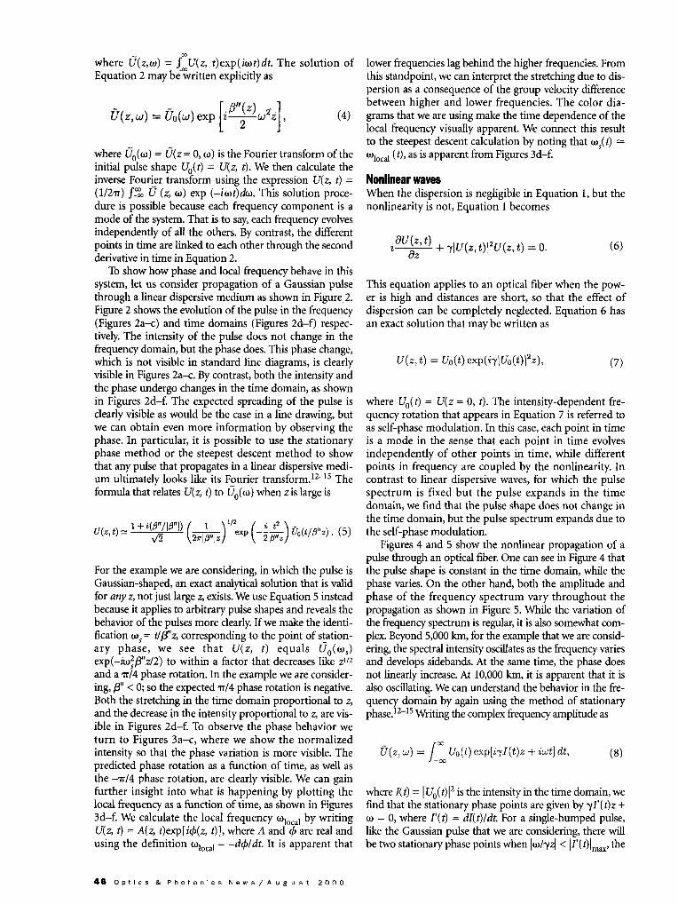
where Ũ(z,ω) = ∫∞

-∞U(z, t)exp(iωt)dt. The solution of Equation 2 may be written explicitly as

where Ũ0(ω) = Ũ(z= 0, ω) is the Fourier transform of the initial pulse shape U0(t) = U(z, t). We then calculate the inverse Fourier transform using the expression U(z, t) = (1/2π) ∫-∞

∞ Ũ (z, ω) exp (-iωt)dω. This solution proce­dure is possible because each frequency component is a mode of the system. That is to say, each frequency evolves independently of all the others. By contrast, the different points in time are linked to each other through the second derivative in time in Equation 2.

To show how phase and local frequency behave in this system, let us consider propagation of a Gaussian pulse through a linear dispersive medium as shown in Figure 2. Figure 2 shows the evolution of the pulse in the frequency (Figures 2a-c) and time domains (Figures 2d-f) respec­tively. The intensity of the pulse does not change in the frequency domain, but the phase does. This phase change, which is not visible in standard line diagrams, is clearly visible in Figures 2a-c. By contrast, both the intensity and the phase undergo changes in the time domain, as shown in Figures 2d-f. The expected spreading of the pulse is clearly visible as would be the case in a line drawing, but we can obtain even more information by observing the phase. In particular, it is possible to use the stationary phase method or the steepest descent method to show that any pulse that propagates in a linear dispersive medi­um ultimately looks like its Fourier transform. 1 2 - 1 5 The formula that relates U(z, t) to Ũ0(ω) when z is large is

For the example we are considering, in which the pulse is Gaussian-shaped, an exact analytical solution that is valid for any z, not just large z, exists. We use Equation 5 instead because it applies to arbitrary pulse shapes and reveals the behavior of the pulses more clearly. If we make the identi­fication ωs = t/β"z, corresponding to the point of station­ary phase, we see that U(z, t) equals Ũ0(ωs) exp(-iω2

sβ"z/2) to within a factor that decreases like z1/2

and a π/4 phase rotation. In the example we are consider­ing, β" < 0; so the expected π/4 phase rotation is negative. Both the stretching in the time domain proportional to z, and the decrease in the intensity proportional to z, are vis­ible in Figures 2d-f. To observe the phase behavior we turn to Figures 3a-c, where we show the normalized intensity so that the phase variation is more visible. The predicted phase rotation as a function of time, as well as the -π/4 phase rotation, are clearly visible. We can gain further insight into what is happening by plotting the local frequency as a function of time, as shown in Figures 3d-f. We calculate the local frequency ω l o c a l by writing U(z, t) = A(z, t)exp[iФ(z, t)], where A and Ф are real and using the definition ω l o c a l = -dФ/dt. It is apparent that

lower frequencies lag behind the higher frequencies. From this standpoint, we can interpret the stretching due to dis­persion as a consequence of the group velocity difference between higher and lower frequencies. The color dia­grams that we are using make the time dependence of the local frequency visually apparent. We connect this result to the steepest descent calculation by noting that ωs(t) ω l o c a l (t), as is apparent from Figures 3d-f.

Nonlinear waves When the dispersion is negligible in Equation 1, but the nonlinearity is not, Equation 1 becomes

This equation applies to an optical fiber when the pow­er is high and distances are short, so that the effect of dispersion can be completely neglected. Equation 6 has an exact solution that may be written as

where U0(t) = U(z = 0, t). The intensity-dependent fre­quency rotation that appears in Equation 7 is referred to as self-phase modulation. In this case, each point in time is a mode in the sense that each point in time evolves independently of other points in time, while different points in frequency are coupled by the nonlinearity. In contrast to linear dispersive waves, for which the pulse spectrum is fixed but the pulse expands in the time domain, we find that the pulse shape does not change in the time domain, but the pulse spectrum expands due to the self-phase modulation.

Figures 4 and 5 show the nonlinear propagation of a pulse through an optical fiber. One can see in Figure 4 that the pulse shape is constant in the time domain, while the phase varies. On the other hand, both the amplitude and phase of the frequency spectrum vary throughout the propagation as shown in Figure 5. While the variation of the frequency spectrum is regular, it is also somewhat com­plex. Beyond 5,000 km, for the example that we are consid­ering, the spectral intensity oscillates as the frequency varies and develops sidebands. At the same time, the phase does not linearly increase. At 10,000 km, it is apparent that it is also oscillating. We can understand the behavior in the fre­quency domain by again using the method of stationary phase. 1 2 - 1 5 Writing the complex frequency amplitude as

where I(f) = |U0(t)|2 is the intensity in the time domain, we find that the stationary phase points are given by үI'(t)z + ω = 0, where I'(t) = dI(t)/dt. For a single-humped pulse, like the Gaussian pulse that we are considering, there will be two stationary phase points when |ω/үz| < |I'(t)|max, the

46 O p t i c s & P h o t o n i c s N e w s / A u g u s t 2 0 0 0

Figure 2. Propagation of a Gaussian pulse through a linear dispersive medium. The dispersion is β" = -0.20 p s 2 / k m , and the full width at half maximum (FWHM) is 20 ps. Figures 2a, 2b and 2c show the pulse profile in the frequency domain at 0, 5,000, and 10,000 km from the launching point. Figures 2d, 2e, and 2f show the pulse profile in the time domain at 0, 5,000, and 10,000 km from the launching point. Color represents phase.

maximum value of |I'(t)| Conversely, when lω/γzl > |I'(f)|max, there are no stationary phase points, and we expect the spectral intensity to rapidly diminish when |ω| becomes larger than its allowed value, as shown in Figure 5. When two stationary phase points exist, we may write the complex frequency amplitude approximately as

when z is large, where I"(t1) and I"(t2) are the second derivatives of I(t) evaluated at the stationary phase points. We see that the contributions from the two sta­tionary phase points will interfere, leading to the ampli­tude and phase oscillations visible in Figure 5. Moreover, Equation 9 implies that the spectral intensity will dimin­ish on average as 1/z while it spreads proportional to z. Both these trends are visible in Figure 5.

An important feature of self-phase modulation is that it induces a chirp in the time domain. Due to the nonlinear phase rotation, apparent in Equation 7 and in Figure 4, the phase varies quadratically near the peak of the pulse. This quadratic variation of the phase translates into a linear vari­ation of the local frequency, as is visible in Figure 6. This chirp can interact in important ways with dispersive ele­

ments. For example, it is possible to at least partially cancel the effect of the nonlinearity with a dispersive element that moves the local frequencies in just the opposite way as the chirp. In the case of solitons, this cancellation is total.4,16 We will have more to say on this subject in the next section.

Nonlinear dispersive waves and solitons In the previous two sections, we discussed the effects of dis­persion and nonlinearity separately. Both these effects con­tinually change the phase of the field, as was clearly visible in our color plots, so that there is no stable pulse solution. In the case of linear dispersive waves, the sign of the dispersion determines the sign of the phase change. By using dispersion with β" < 0, it is possible for the dispersion and the nonlin­earity to induce opposite phase changes that compensate for each other and lead to a stable solution for U(z, t) in which there is no spreading in either the time domain or the fre­quency domain. This solution to Equation 1 is

where A and ω are free parameters proportional to the soliton energy and frequency offset. This solution is called a soliton.8 ,9 ,16 Solitons have the same local fre­quency at all points in time. A remarkable properly of the soliton is that if the

-

Figure 3. Propagation of a Gaussian pulse through a linear dispersive medium. The dispersion is the same as in Figure 2. Figures 3a, 3b, and 3c show the pulse profile in the time domain at 0, 5,000, and 10,000 km from the launching point. Color in these figures represents phase. Figures 3d, 3e, and 3f show the pulse profile in the time domain at 0, 5,000, and 10,000 km from the launching point. Note that 1 Hz = 2 π rad/s, and the color represents local frequency. Intensities in all figures are normalized to the maximum intensity of the pulse.

Optics & Photonics News/August 2000 47

tial pulse differs somewhat from a soliton, the pulse tends to acquire the soliton shape and a uniform phase by shed­ding dispersive radiation. Figure 7 illustrates the propaga­tion of a pulse generated as a coherent sum of three Gaussian pulses slightly shifted with respect to each other. One can see that the input pulse gradually reshapes, approaching the hyperbolic secant soliton shape with a constant local frequency across its profile. The color plots are effective in showing the evolution of the pulse's shape and local frequency as the pulse sheds radiation. Figure 8 shows the corresponding frequency domain evolution. There is no long-term stability in this case because the soliton and the dispersive wave radiation interfere, although the oscillations in the frequency domain become faster and faster with longer propagation distances. The frequency spectrum converges very slowly because the soliton and the dispersive wave radiation interfere. More­over, we use periodic boundary conditions in our numeri­cal solutions, and, in this case, the frequency spectrum never converges. To avoid this problem, it is necessary to

actually damp out the dispersive waves in order for the pulse profile to stabilize in the frequency domain. We used a time domain much larger than the time domain shown in our simulations, along with a numerical damper at the edges, to avoid boundary interactions.

Dispersion managed soliton Dispersion by itself causes the different frequency com­ponents of a pulse to travel with different velocities so that a propagating pulse may compress or expand in the time domain. Whether higher or lower frequencies move faster depends on the sign of the dispersion. A fiber with alternating spans of normal (β" > 0) and anomalous (β" < 0) dispersion thus leads to alternating stages of expansion and compression of an optical pulse. When nonlinearity is present, this effect can lead to a periodi­cally stationary pulse whose shape and local frequency return to their original values after one period. This pulse is called a dispersion managed soliton.10,11

Figure 9 shows one example of the evolution of a dis-

Figure 4 . Propagation of a Gaussian pulse through a nonlinear medium without dispersion. The medi­um's nonlinear coefficient is γ = 2.1 W-1 k m - 1 , cor­responding to a fiber with n 2 = 2.6 x 10-20 m 2 / W , Aeff = 50 μ m 2 , and λ 0 = 2 π c / ω 0 = 1.55 μ m . The peak power is 0.38 mW, and the F W H M is 20 ps. Figures 4a , 4b, and 4c show the pulse profile in the time domain at 0, 5,000, and 10 ,000 km from the launching point. Color represents phase.

Figure 5. Propagation of a Gaussian pulse through a nonlinear medium without dispersion. Parame­ters are the same a s in Figure 4. Figures 5a , 5b and 5c show the pulse profile in the frequency domain at 0, 5 ,000, and 10 ,000 km from the launching point. Color represents phase.

Figure 6. Propagation of a Gaussian pulse through a nonlinear medium without dispersion. Parameters are the same a s in Figure 4. Figures 6a , 6b and 6c show the pulse profile in the t ime domain at 0, 5 ,000, and 10 ,000 km from the launching point. Color represents local frequency.

48 Optics & Photonics News/August 2000

persion managed soliton. Figure 10 shows the dispersion map for this example. It consists of equal length spans of normal and anomalous dispersion with almost but not quite the same absolute values of dispersion. We first com­pare the pulse at the beginning and at the end of the dis­persion map (Figures 9a and 9e). It is apparent that the pulse conserves its shape and that the frequency distribu­tion remains uniform. Hence, the pulse is periodically sta­tionary. Since the first quarter of the dispersion map

(0 < z < L/4) consists of fiber with anomalous dispersion, the pulse should expand in the time domain, as is observed in Figure 9b, which represents the pulse at the interface of the anomalous and normal spans (z = L/4). The local fre­quency range is about ± 100 GHz, and the pulse expands to about twice its initial duration. The next two quarters of the map (L/4 < z < 3L/4) consist of normal dispersion fiber. As expected, the pulse first compresses and then expands again with the opposite phase and local frequency

Figure 7. Propagation of a pulse through a medium with both dispersion and nonlinearity. The parame­ters are: β" = - 2 0 p s 2 / k m and γ = 1.3W-1 Km-1, cor­responding to a fiber with Aeff = 8 0 μ m 2 and the oth­er parameters as in Figure 4. Figures 7 a - 7 e show the pulse profile in the t ime domain at 0, 20 , 50 , 500, and 10 ,000 km respectively from the launch­ing point. Color represents local frequency. The ini­tial pulse is a coherent sum of three Gaussian puls­es. The central pulse has an initial peak power of 14 mW and a F W H M of 4 6 ps. Another pulse is delayed by F W H M / 3 and its power is reduced by √2 with respect to the central pulse. The third pulse is analogous to the second one except that it is ahead of the central pulse by F W H M / 3 .

Figure 8. Propagation of a pulse through a medi­um with both dispersion and nonlinearity. Parame­ters are the s a m e a s in Figure 7. Here, we show the evolution in the frequency domain. Color rep­resents phase.

Figure 9. Propagat ion of a d ispers ion-managed soli-ton through the d ispers ion m a p shown in Figure 1 0 . The nonlinear coef f ic ient γ = 1.3 W-1 k m - 1 . Co l ­or represents local f requency. The initial peak pow­er of the pulse is 3.2 mW.

Optics & Photonics News/August 2000 49

Figure 10. Dispersion map used for the example in Figure 9 . The total length L = L1 + L2 is 200 km. It c o n s i s t s of equal lengths of normal and anomalous dispersion s p a n s (L1 = L2 = 1 0 0 km). The dispersion coef f ic ients in the normal and anomalous dispersion s p a n s are respectively β"1 = -10 .99 ps2/km and β"2 = 11 .01 ps2/km. The average dispersion for this map is β" = 0 .001 ps2/km.

at any point in time. Figure 9c shows the pulse in the mid­dle of the normal dispersion span. It is compressed and has a uniform frequency distribution. Figure 9d shows the pulse at the end of the normal span (z = 3L/4). The pulse has expanded and its local frequency distribution is just the opposite of what is observed in Figure 9b at z= L/4. Final­ly, the last quarter of the map consists of anomalous dis­persion fiber. Hence, as seen in Figure 9e, the pulse com­presses back to its original shape and regains its original uniform frequency distribution.

Conclusion Any wave is characterized by both its amplitude and its phase. Standard line drawings are fine for representing amplitude but do a poor job of representing phase. By using false color to represent the phase or the local fre­quency underneath an envelope that represents the inten­sity, it is possible to obtain an immediate, visual insight into the total wave evolution. Comparing these color plots to the formulae produced by standard analytical tools like the stationary phase method or the steepest descent method allows us to better understand these well-known, classical formulae. It is our view that as color monitors, video projectors, and color printers become increasingly accessible, the approach that we have outlined should become a paradigm for how to effectively represent the evolution of waves.

References 1. L.G. Kazovsky, et al., Optical Fiber Communication Sys­

tems, (Artech House, Boston, 1996). 2. A. Hill, "Enabling continued internet growth at the speed

of light," PennWell, 17(6), (May 2000). See also www.light-wave.com.

3. S. Clavenna, "The expanding optical-network market: More carriers, more diversity," PennWell, 17(6) (May 2000). See also www.light-wave.com

4. G.P. Agrawal, Nonlinear Fiber Optics (Academic, San Diego, 1995).

5. Y.R. Shen, Principles of Nonlinear Optics (Wiley, New York, 1984).

6. F. Shimizu, "Frequency broadening in liquids by a short light pulse," Phys. Rev. Lett., 19, 1097 (1967).

7. T.K. Gustafson, et al., "Self-modulation, self-steepening, and spectral development of light in small-scale trapped fil­aments," Phys. Rev., 177, 306 (1969).

8. A. Hasegawa and F. Tappert, "Transmission of stationary nonlinear optical pulses in dispersive dielectric fibers. I. Anomalous dispersion," Appl. Phys. Lett., 23, 142 (1973).

9. L.F. Mollenauer, et al., "Experimental observation of picosecond pulse narrowing and solitons in optical fibers," Phys. Rev. Lett., 4 5 , 1095 (1980).

10. N.J. Smith, et al., "Enhanced power solitons in optical fibers with periodic dispersion management," Electron. Lett., 32, 54 -5 (1996).

11. I. Morita, et al., "20 G b / s single-channel soliton transmis­sion over 9000 km without inline filters," Photon. Technol. Lett., 8, 1573-4 (1996).

12. P.M. Morse and H. Feshbach, Methods of Theoretical Physics, Part / (McGraw-Hill, New York, 1953), Chap. 4.6, pp. 434-43.

13. G. Arfken, Mathematical Methods for Physicists (Academ­ic, San Diego, 1985), Chap. 7.4, pp. 428-34 .

14. N. Bleistein and R.A. Handelsman, Asymptotic Expansions of Integrals (Dover, New York, 1986), Chap. 6.1, pp. 219-24 and Chaps. 7.1-7.2, pp. 252-80 .

15. F.W.J. Olver, Asymptotics and Special Functions (A.K. Peters, Wellesley, MA, 1997), Chap. 3.11-3.13, pp. 96-104 and Chap. 4.10, pp. 135-7 .

16. A. Hasegawa and Y. Kodama, Solitons in Optical Communi­cations (Clarendon, Oxford, 1995).

17. M. Nakazawa and H. Kubota, "Optical soliton communication in a positively and negatively dispersion allocated optical fiber transmission line," Electron. Lett., 31(3), 216-17 (1995).

G.V. Grigoryan, I.T. Lima, Jr., T. Yu, V.S. Grigoryan and C.R. Menyuk all contributed to this paper while at the Department of Computer Science and Electrical Engineering, University of Maryland Baltimore County (UMBC). G. Grigoryan is an undergraduate at UMBC, majoring in computer science and biology. I. Lima is a graduate research assistant in the electrical engineering program at UMBC. T. Yu is a research scien­tist at Qtera Corporation and V. Grigoryan is a research scientist at Corvis Corpora­tion. C. Menyuk, a professor in the Computer Science and Electrical Engineering Department at UMBC, is currently on leave, working at the Laboratory for Telecom­munications Sciences in Adelphi, MD. To contact the first author, use the email address: ggrigo1@gl.umbc.edu.

50 Optics & Photonics News/August 2000

How we did it There are many ways to generate color plots like the ones shown here. In this article, we proceeded as follows.

The numerical solutions that we show were obtained from Equation (4) for linear, dispersive transmission and from Equation (7) for non-linear transmission without dis­persion. When both dispersion and non-linearity were pre­sent, we solved Equation (1) with the split-step Fourier method using computer codes written in FORTRAN and C++. Once we had the data, we used the function PCOL­OR in the widely used, commercial software package MATLAB. To use PCOLOR, one must specify a color map, but MATLAB has several built-in color maps to make the job easier. We used HSV for our periodic color map to represent phase, and we used JET for our aperiodic color map to represent the local frequency.

We have been presenting animated versions of the fig­ures shown here at scientific meetings. To generate the

animations, we create a series of JPEG files using MAT­LAB, labeled sequentially as fig1.jpg, fig2.jpg, fig3.jpg, etc. Using QuickTime Pro 4.0, available commercially from Apple, we generate .mov files. A word of caution: we typically include the animations inside PowerPoint files for presentation at meetings. To do that successfully with a Microsoft operating system, one must first install an older version of QuickTime, QuickTime 2.1, on the sys­tem. The older version of QuickTime is not downloadable from Apple's web site. We obtained it from an Adobe Illus­trator CD. (No doubt, the incompatibility of QuickTime 4.0 and PowerPoint is a feature, not a bug.)

The MATLAB script files that we used to create the figures and animated versions of some of the figures are available at the URL: http://www.photonics.umbc. edu/UsingColors.html.