Using artificial intelligence algorithms for high level ...orlabanalytics.ca/jaor/archive/v9/n1/jaorv9n1p11.pdf · Using artificial intelligence algorithms for high level tactical

Journal of Applied Operational Research (2017) Vol. 9, No. 1, 11–26 ISSN 1735-8523 (Print), ISSN 1927-0089 (Online)

www.orlabanalytics.ca

Using artificial intelligence algorithms for high level tactical wargames and new approaches to wargame simulation

S.G. Lucek 1, and S.J. Collander-Brown

2

1 Newman & Spurr Consultancy Ltd (NSC), Surrey, UK 2 Defence Science and Technology Laboratory (Dstl), Fareham, UK

Received 06 October 2016 Accepted 22 August 2017

Abstract—The Mission Planner is a decision-making toolset developed by NSC, a UK based provider of

cutting‑edge training, modelling and simulation and consultancy services, for Dstl (Defence Science and

Technology Laboratory, an executive agency, sponsored by the UK Ministry of Defence) currently applied

at the tactical level of combat. It aims to support Dstl high intensity warfighting simulations by reducing or

eliminating the need for complex pre-scripting of simulated combat units or human-in-the-loop interactors.

This has a big impact in reducing the burden of supporting simulations needed for Dstl studies. Two stochastic

optimisation Artificial Intelligence (AI) techniques have been used (Genetic Programming and a novel

implementation of Simulated Annealing). The algorithms have been employed in a generic architecture

that allows simple application to different problems. This is central to the approach taken. The problem

considered is the Dstl level land engagement simulation, SimBrig. This is a highly detailed and complex

simulation, with execution times that prohibits the many runs required for the AI to consider a wide range

of possible solutions (in this case orders for the military units under AI control). Also, application of

stochastic optimisation AI directly on this model would result in solutions that exploited the detailed

complexities of the engagement simulation, rather than were based on sound tactical reasoning. However,

being able to switch the AI between problems means that a solution can be quickly generated against a

simplified wargame (a meta model) which represents only the essential elements of the full wargame

problem, whilst still referencing the full simulation (SimBrig) to evaluate the quality of the solution as

necessary. The meta model is designed to be quick and robust, without the complexities that would be

exploited by the AI. However all essential elements of the tactical problem are modelled (albeit as simply

as possible) so that the solutions considered by the AI are properly evaluated. A novel approach has been

taken in the way the problem is formulated for the AI. Presenting the problem to the AI using military-like

syntax results in the AI algorithms efficiently generating plans for tactical problems which resemble

human decision making. This paper presents the approach and techniques used in both the AI algorithms

and the meta wargame simulation.

Published online 17 October 2017

Copyright © ORLab Analytics Inc. All rights reserved.

Keywords:

Artificial intelligence

Combat modelling

Genetic algorithms

Genetic programming

Simulated annealing

Stochastic optimisation

Strategic game

Wargame simulation

Introduction

The Mission Planner is a decision-making toolset developed by NSC for use in Dstl

high intensity warfighting simulations.

It automatically develops plans for allocating forces in space and time in order to achieve a particular objective, in a situation

of partial knowledge and where the enemy is also planning and reacting. Traditionally Dstl models have approached such

problems by building complex pre-scripted orders or by using a human-in-the-loop solution. These approaches can, in

principle, represent human decision making in a reasonably accurate manner but at the cost of time (and therefore money)

in the set up and/or running of the model. Such constraints can severely limit their practical application.

The Mission Planner has been developed to use two different stochastic optimisation AI techniques in order to solve

tactical problems in a number of wargames, so that they can play one or more sides. The programme of work was started

to support the Dstl combat model CLARION, and the AI algorithms have been applied to: a proof-of-concept test bed (in

order to better understand the capabilities and limitations of the algorithms employed); SimBrig; and a bespoke brigade

level land simulation, META (Model for EngagemenT Analysis).

Correspondence: S.G. Lucek, Newman & Spurr Consultancy Ltd,

Norwich House, Knoll Rd, Camberley, Surrey, GU15 3SY, UK

E-mail: [email protected]

Lucek and Collander-Brown (2017)

12

Stochastic Optimisation

Stochastic Optimisation represents a family of techniques for solving any generalised problem. These are often applied to

complex problems, where it is impractical to go through all possible solutions (called the solution space) to determine the

optimum. These techniques randomly explore a subset of the solution space in a rigorous mathematical fashion, to arrive

at a “good” solution to the problem, though not necessarily guaranteed to be the best solution. An important aspect of these

techniques is that they balance exploring avenues that offer promising results with searching the full solution space.

Therefore they are able to find a globally “good” solution rather than be limited to the best solution in a local area of the

solution space. The general approach was first considered by H. Robbins and S. Monro (1951) and is summarised in J. C.

Spall (2003). Traditionally these techniques are applied to a wide range of problems, including wargaming (D. Jackson,

2005) timetabling (Zhao Le, et al., 2014) and scheduling (e.g. the travelling salesmen problem, V. Černý, 1985), game

solutions (e.g. chess: A. Hauptman, M. Sipper 2005 and 2007; black gammon: Y. Azaria, M. Sipper, 2005; soccer bots:

S. Luke, 1998; and robocode: Y. Shichel, et al. 2005) and circuit and antennae design (J.R. Koza et al., 1999, J. Lohn, et

al., 2004).

Genetic Algorithm Overview

Genetic algorithms have a long history of use as an optimisation technique. N.A. Barricelli (1963) simulated evolution

techniques to play a simple game, and the methods are described in books by A. Fraser, D. Burnell (1970). The Genetic

Algorithm technique has an abstract representation of a candidate solution to a problem, referred to as an entity. This is

typically a bit stream, a binary string of 0s and 1s. These are then translated into a solution to a specific problem by a process

called decoding. For a wargame example, the 0s and 1s could translate to a set of orders:

Move 000

Attack 001

Defend 010

Support 011

Retreat from 100

The preceding bits could represent input values to the order, for example the actor or target units, timings, areas etc.

Orders across all the units in the wargame could then be built up from the bit stream. These orders are then evaluated in a

wargame model to obtain a “fitness measure”, a quantitative measure of how good the solution is. A population of entities

is considered, randomly initialised. This population is then evolved in generations, with parent solutions chosen by a

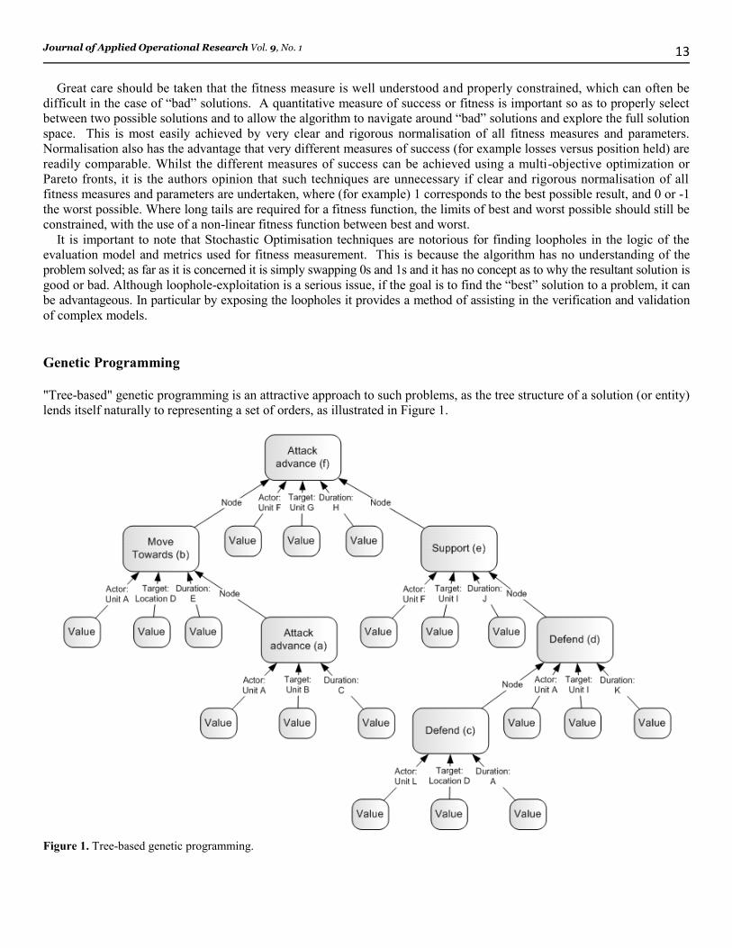
method that mimics survival of the fittest, representing evolutionary pressure. Child solutions are then generated by

mutation and/or crossover of the bit streams of selected parents illustrated in Figures 2 and 3. A ‘best’ (optimized) solution is

then achieved after a number of generations.

The selection of parent solutions is based on a fitness measure applied to each member solution separately, which enables

the population to evolve to fitter solutions in a prescribed way. The selection technique must maintain genetic diversity in

order to arrive at a globally good solution, as a solution might have poor fitness, but have beneficial elements for achieving a

good result later on in the run. Tournament selection is one method that achieves this. When selecting a parent, first a

number of candidates are chosen at random (regardless of their fitness). The best out of these is then selected. This ensures

that a small number of well fitted but related entities are not always selected, to become overly dominant in the population,

and removing diversity of solution.

Fitness Measure

The fitness measure is core to all stochastic optimisation algorithms. A good measure of fitness allows algorithm to

correctly apply selection pressure and ensures fittest elements of population are evolved. For the wargame example, the

fitness measure is obtained by first decoding an entity to a set of orders. These orders are then run through the evaluation

wargame simulation and the results are assessed in terms of losses, achievements (positions held or denied from the enemy,

or enemy losses or neutralisation), risk (enemy proximity and whether own units are mutually supporting), and efficiency

(minimum resource consumption).

Journal of Applied Operational Research Vol. 9, No. 1

13

Great care should be taken that the fitness measure is well understood and properly constrained, which can often be

difficult in the case of “bad” solutions. A quantitative measure of success or fitness is important so as to properly select

between two possible solutions and to allow the algorithm to navigate around “bad” solutions and explore the full solution

space. This is most easily achieved by very clear and rigorous normalisation of all fitness measures and parameters.

Normalisation also has the advantage that very different measures of success (for example losses versus position held) are

readily comparable. Whilst the different measures of success can be achieved using a multi-objective optimization or

Pareto fronts, it is the authors opinion that such techniques are unnecessary if clear and rigorous normalisation of all

fitness measures and parameters are undertaken, where (for example) 1 corresponds to the best possible result, and 0 or -1

the worst possible. Where long tails are required for a fitness function, the limits of best and worst possible should still be

constrained, with the use of a non-linear fitness function between best and worst.

It is important to note that Stochastic Optimisation techniques are notorious for finding loopholes in the logic of the

evaluation model and metrics used for fitness measurement. This is because the algorithm has no understanding of the

problem solved; as far as it is concerned it is simply swapping 0s and 1s and it has no concept as to why the resultant solution is

good or bad. Although loophole-exploitation is a serious issue, if the goal is to find the “best” solution to a problem, it can

be advantageous. In particular by exposing the loopholes it provides a method of assisting in the verification and validation

of complex models.

Genetic Programming

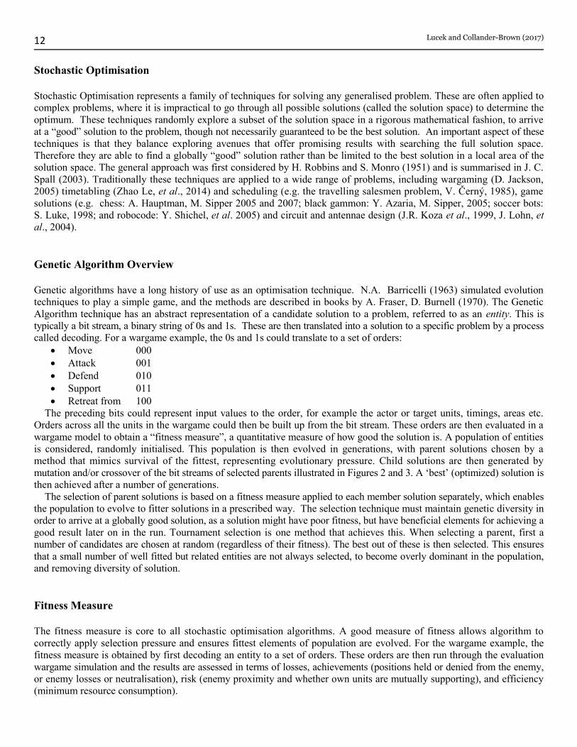
"Tree-based" genetic programming is an attractive approach to such problems, as the tree structure of a solution (or entity)

lends itself naturally to representing a set of orders, as illustrated in Figure 1.

Figure 1. Tree-based genetic programming.


14

The first statement of modern "tree-based" genetic programming was given by N.L. Cramer (1985). The methods are

described in J.R. Koza (1999) and R. Poli, et al. (2008). Genetic Programming is a subset of Genetic Algorithms. The

difference is that, instead of a bit stream of 0s and 1s, a candidate solution is made up of a node/input tree as illustrated in

Figure 1.

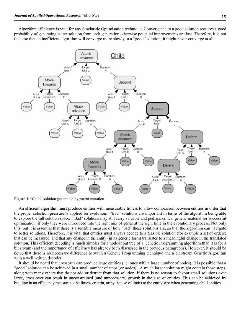
Assuming the simulation starts at a time T, the nodes translate as follows:

Attack advance by actor unit A moving (and attacking if in range) target B, starting at time T ending at time T+C

Unit A moves towards location D, starting at time T+C (the time actor A finishes its previous action represented

by node a) finishing at time T+C+E

Unit L moves towards (and defends if in range) location D starting at time T and ending at time T+A

Unit A moves towards (and defends if in range) unit I, starting at time T+C+E (the time actor A finishes its previous

action represented by node b) and ending at time T+C+E+K)

Unit F moves towards (and supports if in range) unit I, starting at time T and ending at time T+J

Unit F moves towards (and attacks if in range) target G, starting at time T+J (the time actor F finishes its previous

action represented by node e) and ending at time T+J+H

It is important to note that whilst a wargame example has been illustrated, in a Genetic Algorithm an entity is simply a

node/input tree, each node having a number of input values and node children. The algorithm has no concept of what a

node or input might mean, and it is only at the decoder stage that it is determined how each node translates to an order. In

principle, there is no difference between the mathematics of a bit stream Genetic Algorithm and a node/input tree Genetic

Programming algorithm. However, it is much easier to write a decoder that efficiently translates the entity, in its generic

form, to a solution for a particular problem.

.

Figure 2. “Child” solution generation from parent entities by crossover.


15

Algorithm efficiency is vital for any Stochastic Optimisation technique. Convergence to a good solution requires a good

probability of generating better solution from each generation otherwise potential improvements are lost. Therefore, it is not

the case that an inefficient algorithm will converge more slowly to a “good” solution; it might never converge at all.

Figure 3. “Child” solution generation by parent mutation.

An efficient algorithm must produce entities with measurable fitness to allow comparison between entities in order that

the proper selection pressure is applied for evolution. “Bad” solutions are important in terms of the algorithm being able

to explore the full solution space. “Bad” solutions may still carry valuable and perhaps critical genetic material for successful

optimization, if only they were introduced into the right mix of genes at the right time in the evolutionary process. Not only

this, but it is essential that there is a sensible measure of how “bad” these solutions are, so that the algorithm can navigate

to better solutions. Therefore, it is vital that entities must always decode to a feasible solution (for example a set of orders)

that can be measured, and that any change in the entity (in its generic form) translates to a meaningful change in the translated

solution. This efficient decoding is much simpler for a node/input tree of a Genetic Programming algorithm than it is for a

bit stream (and the importance of efficiency has already been discussed in the previous paragraphs). However, it should be

noted that there is no necessary difference between a Genetic Programming technique and a bit stream Genetic Algorithm

with a well written decoder.

It should be noted that crossover can produce large entities (i.e. ones with a large number of nodes). It is possible that a

“good” solution can be achieved in a small number of steps (or nodes). A much larger solution might contain those steps,

along with many others that do not add or detract from that solution. If there is no reason to favour small solutions over

large, cross-over can result in unconstrained (and unnecessary) growth in the size of entities. This can be achieved by

building in an efficiency measure to the fitness criteria, or by the use of limits to the entity size when generating child entities.


16

Simulated Annealing

Simulated Annealing is a well understood and efficient optimisation technique, which shares many similar elements to

Genetic Algorithms. The earliest form of this algorithm is the Metropolis-Hastings algorithm, N. Metropolis, et al.

(1953). The method is described in detail in W.H. Press (2007). The concepts are analogous in form to annealing in

metallurgy, a technique where heating and controlled cooling of a material increases the size of crystals and reduces

defects in the atomic lattice. It uses the same mathematics as determining probability states given the thermodynamic free

energy. As the Boltzmann distribution is mathematically well understood, the process is much better defined than the

heuristic approach of Genetic Algorithms.

A candidate solution is considered, which can be formulated using the same generic representation as the Genetic

approaches. A single solution is considered throughout the process, rather than a population. This solution is randomly

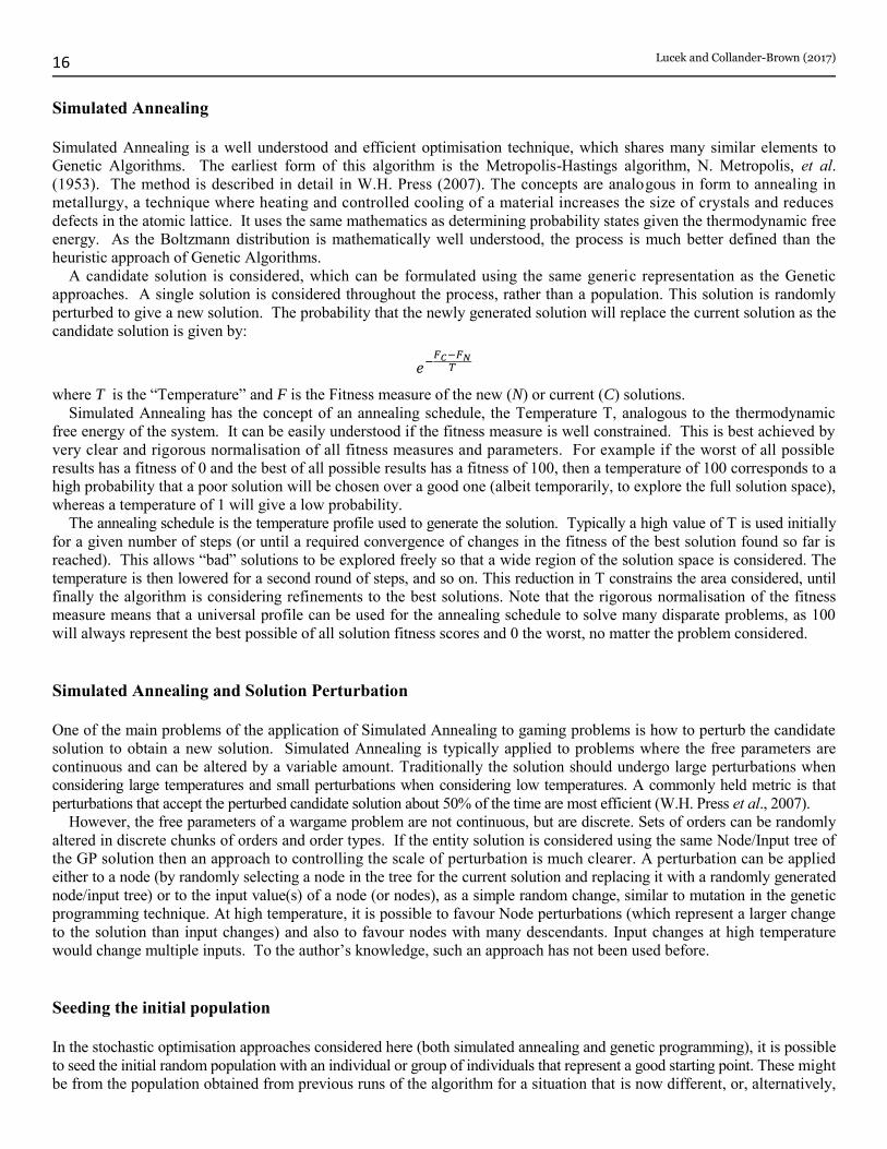
perturbed to give a new solution. The probability that the newly generated solution will replace the current solution as the

candidate solution is given by:

where T is the “Temperature” and F is the Fitness measure of the new (N) or current (C) solutions.

Simulated Annealing has the concept of an annealing schedule, the Temperature T, analogous to the thermodynamic

free energy of the system. It can be easily understood if the fitness measure is well constrained. This is best achieved by

very clear and rigorous normalisation of all fitness measures and parameters. For example if the worst of all possible

results has a fitness of 0 and the best of all possible results has a fitness of 100, then a temperature of 100 corresponds to a

high probability that a poor solution will be chosen over a good one (albeit temporarily, to explore the full solution space),

whereas a temperature of 1 will give a low probability.

The annealing schedule is the temperature profile used to generate the solution. Typically a high value of T is used initially

for a given number of steps (or until a required convergence of changes in the fitness of the best solution found so far is

reached). This allows “bad” solutions to be explored freely so that a wide region of the solution space is considered. The

temperature is then lowered for a second round of steps, and so on. This reduction in T constrains the area considered, until

finally the algorithm is considering refinements to the best solutions. Note that the rigorous normalisation of the fitness

measure means that a universal profile can be used for the annealing schedule to solve many disparate problems, as 100

will always represent the best possible of all solution fitness scores and 0 the worst, no matter the problem considered.

Simulated Annealing and Solution Perturbation

One of the main problems of the application of Simulated Annealing to gaming problems is how to perturb the candidate

solution to obtain a new solution. Simulated Annealing is typically applied to problems where the free parameters are

continuous and can be altered by a variable amount. Traditionally the solution should undergo large perturbations when

considering large temperatures and small perturbations when considering low temperatures. A commonly held metric is that

perturbations that accept the perturbed candidate solution about 50% of the time are most efficient (W.H. Press et al., 2007).

However, the free parameters of a wargame problem are not continuous, but are discrete. Sets of orders can be randomly

altered in discrete chunks of orders and order types. If the entity solution is considered using the same Node/Input tree of

the GP solution then an approach to controlling the scale of perturbation is much clearer. A perturbation can be applied

either to a node (by randomly selecting a node in the tree for the current solution and replacing it with a randomly generated

node/input tree) or to the input value(s) of a node (or nodes), as a simple random change, similar to mutation in the genetic

programming technique. At high temperature, it is possible to favour Node perturbations (which represent a larger change

to the solution than input changes) and also to favour nodes with many descendants. Input changes at high temperature

would change multiple inputs. To the author’s knowledge, such an approach has not been used before.

Seeding the initial population

In the stochastic optimisation approaches considered here (both simulated annealing and genetic programming), it is possible

to seed the initial random population with an individual or group of individuals that represent a good starting point. These might

be from the population obtained from previous runs of the algorithm for a situation that is now different, or, alternatively,


17

they might be constructed by the user. There is a danger that if the seed individuals are much better than the randomly

created trees, then their descendants can take over the population rapidly with a loss of genetic diversity. In these cases it

is often more successful to control this diversity loss by initialising the whole population to either identical or mutated

copies of the seed individuals. The Mission planner toolset allows saving entity solutions (in their generic form) to a plan

store. These stored plans represent a library of solutions which can then be used as seed solutions for future runs of the toolset.

Stochastic Optimisation

Stochastic Optimisation techniques, traditionally, have a number of limitations. First, they can be slow, considering very

many possible solutions. If a long time is required to evaluate how good each solution, then these techniques might become

prohibitive. Typically, for a brigade level problem, it might require evaluation of some tens of thousands of possible solutions

to reach a reasonable solution. Even if each evaluation takes a millisecond this would mean the time taken for a solution

would be measured in tens of seconds.

Also, the algorithms have no concept or understanding as to why a solution might be good, traditionally regarded as

strength of these techniques. This has a tendency of generating solutions in response to the exact detail of the problem

posed, rather than necessarily a solution that is applicable to a wide range of problems. This makes these techniques

excellent at, for example, circuit or antennae design (J.R. Koza et al., 1999, J. Lohn, et al., 2004), where they are able to

come up with novel solutions that are not naturally intuitive. However, they are not necessarily suitable for arriving at

doctrinally correct solutions that reflect the perceived wisdom of, for example, the Staff Officers Handbook, for a

wargame problem, unless heavily constrained.

As discussed above Stochastic Optimisation techniques are also famous for exploiting loopholes in the problem posed.

These might be in the fitness criteria by which a solution is assessed, or else in the logic of the evaluation model. This arises,

again, from the fact that the algorithms have no concept or understanding as to why a solution is good. Any implementation

of these techniques will have to take into account these limitations, either accepting them, or finding solutions.

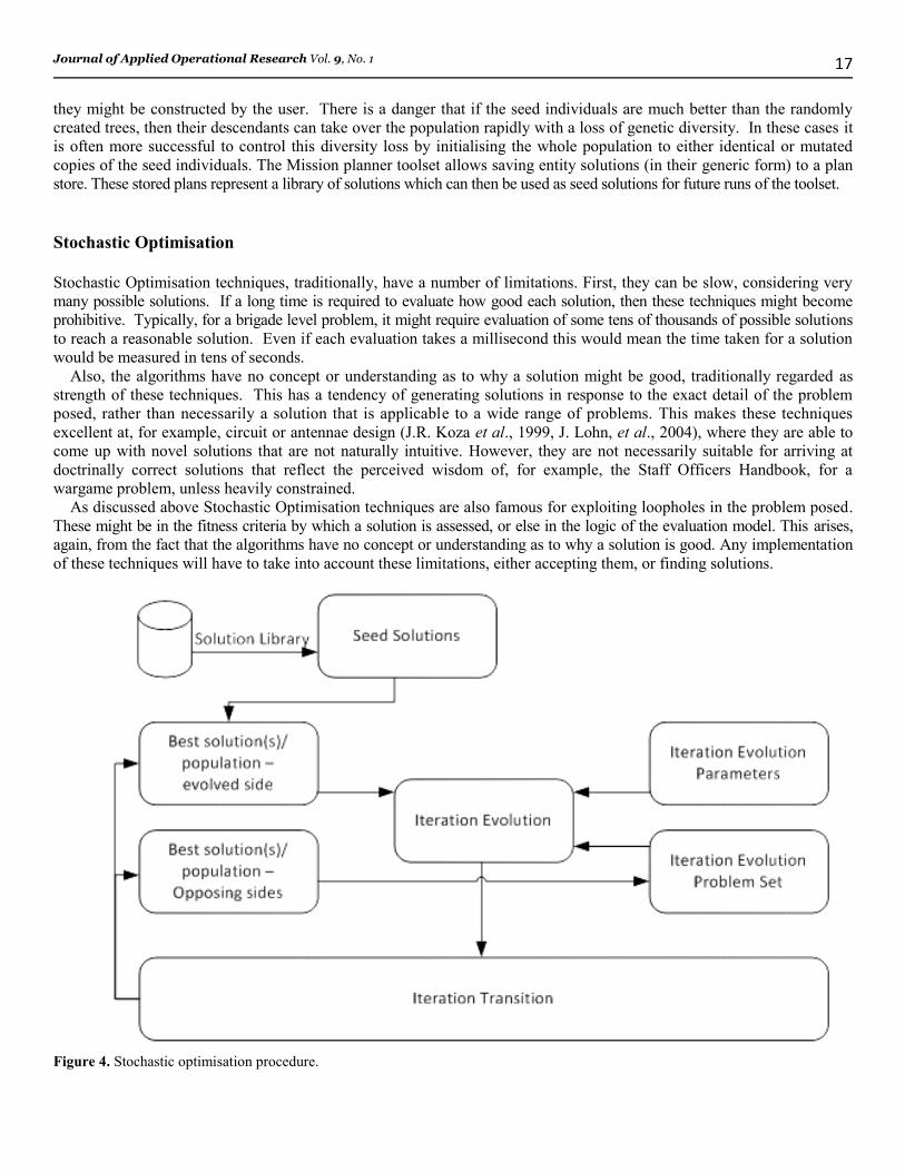
Figure 4. Stochastic optimisation procedure.


18

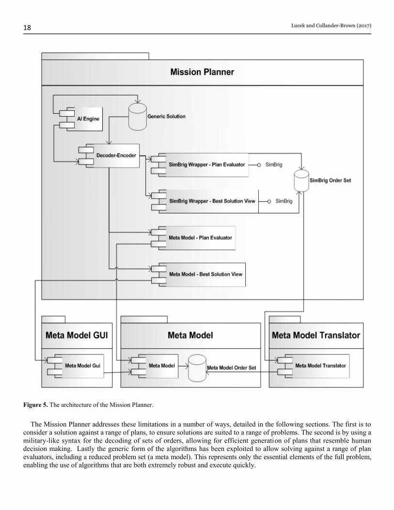
Figure 5. The architecture of the Mission Planner.

The Mission Planner addresses these limitations in a number of ways, detailed in the following sections. The first is to

consider a solution against a range of plans, to ensure solutions are suited to a range of problems. The second is by using a

military-like syntax for the decoding of sets of orders, allowing for efficient generation of plans that resemble human

decision making. Lastly the generic form of the algorithms has been exploited to allow solving against a range of plan

evaluators, including a reduced problem set (a meta model). This represents only the essential elements of the full problem,

enabling the use of algorithms that are both extremely robust and execute quickly.


19

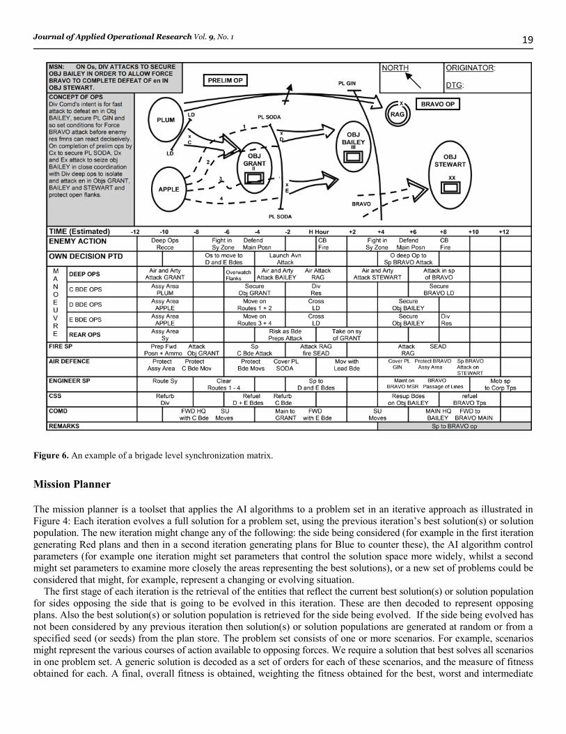
Figure 6. An example of a brigade level synchronization matrix.

Mission Planner

The mission planner is a toolset that applies the AI algorithms to a problem set in an iterative approach as illustrated in

Figure 4: Each iteration evolves a full solution for a problem set, using the previous iteration’s best solution(s) or solution

population. The new iteration might change any of the following: the side being considered (for example in the first iteration

generating Red plans and then in a second iteration generating plans for Blue to counter these), the AI algorithm control

parameters (for example one iteration might set parameters that control the solution space more widely, whilst a second

might set parameters to examine more closely the areas representing the best solutions), or a new set of problems could be

considered that might, for example, represent a changing or evolving situation.

The first stage of each iteration is the retrieval of the entities that reflect the current best solution(s) or solution population

for sides opposing the side that is going to be evolved in this iteration. These are then decoded to represent opposing

plans. Also the best solution(s) or solution population is retrieved for the side being evolved. If the side being evolved has

not been considered by any previous iteration then solution(s) or solution populations are generated at random or from a

specified seed (or seeds) from the plan store. The problem set consists of one or more scenarios. For example, scenarios

might represent the various courses of action available to opposing forces. We require a solution that best solves all scenarios

in one problem set. A generic solution is decoded as a set of orders for each of these scenarios, and the measure of fitness

obtained for each. A final, overall fitness is obtained, weighting the fitness obtained for the best, worst and intermediate


20

individual scores. This ensures that the solution obtained is good against a wide variety of scenarios and is not limited to

the specific details of a single scenario. It also permits solution of scenarios where there is uncertainty in the problem

posed, for example, if Blue has does not have a clear view of Red forces, a number of scenarios could be considered.

Mission Planner, Generic Architecture

As has been discussed, the AI algorithms work with a completely generic form of solution that can be applied to any problem.

The only problem-specific element is the decoder, which takes a solution, in its generic form, and translates it to a solution

for a specific problem, in this case a set of orders for a wargame simulation.

This specific solution is then evaluated to obtain a fitness score, which the AI algorithm then stores against the generic

form of the solution to determine its use in exploring the full problem space. The architecture of the Mission Planner exploits

the generic nature of the algorithms employed to allow it to consider any problem, as illustrated in Figure 5. Decoders can

be written in a plug and play fashion to consider problems of a completely different form. The inter-changeability of

decoders means that one decoder can be used to assess solutions during the solution evolution process (the plan evaluator),

whilst a different decoder can be used to view and assess the best solution arrived at (the solution view). Figure 5 demonstrates

this with decoders for plan evaluation and solution views for both the META model and SimBrig.

Military Syntax

The mission planner uses a military-like syntax for decoding of sets of order, i.e. for translating a generic solution into a

set of orders. This method is currently used for both the SimBrig and META decoders. The concepts in a military synch

matrix are used, an example of which is illustrated in Figure 6.

The nodes in the generic solution are translated into Areas and Timelines and Manoeuvre/Support orders. The inputs

determine which locations correspond to each area in the solution, and the times of the timelines. Inputs for each Manoeuvre/

Support order determine which areas and timelines are associated with that Manoeuvre/Support order.

In this way units naturally co-operate in time and space. By using this military syntax, the set of orders generated naturally

looks human-like. It also greatly enhances efficiency. For example, it can readily be seen that a “generically” good set of

orders can be generated, which determines how units are to co-operate, by the way each unit’s orders are linked to areas

and timelines. A solution that is good for one problem can be applied to a different problem simply by changing the

specifics of the locations of the areas and the timings of the timelines. The AI algorithms will exploit such efficiencies

when randomly generating solutions. To the authors knowledge this is the first time that the use of military syntax has

been used for Stochastic Optimisation algorithms applied to a wargame problem.

META

The META wargame model is a bespoke model to evaluate a brigade level land engagement. It has been specifically

developed to meet the requirements of the AI algorithms of the Mission Planner, which are for a plan evaluation model

that is fast and robust, i.e. has no loopholes in the logic of its evaluation algorithms and that will also successfully evaluate

all sets of orders, no matter how nonsensical they might seem. This is important for the AI algorithms, as they need to

consider “bad” solutions, to be able to assign a quantitative measure of fitness to enable the algorithm to navigate to

“good” solutions whilst still exploring the full solution space.

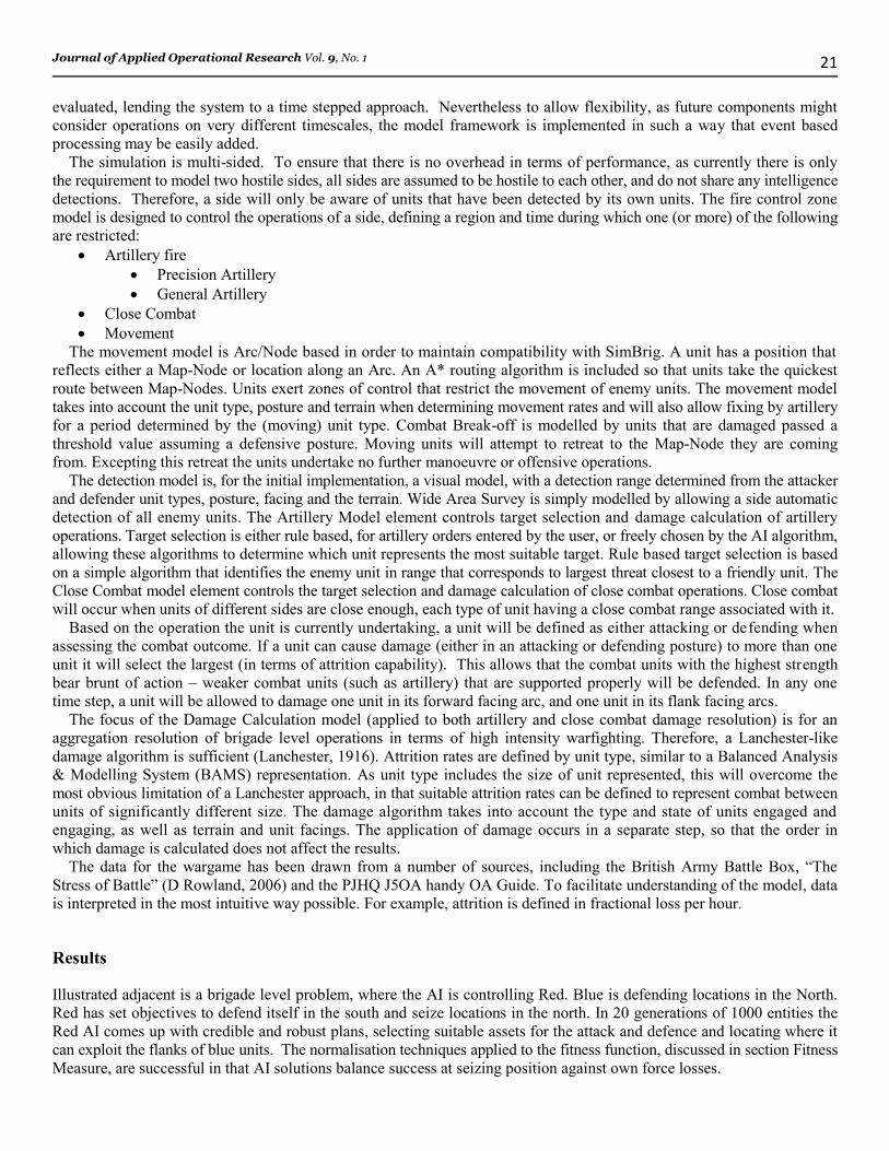
The guiding principle of the META model has been simplicity. The algorithms have been streamlined to represent only

the essential elements of the full problem, in order to avoid unintentional complexity. This minimises loopholes in the

logic of the wargame which would be exploited by the AI algorithms. The simplicity of the approach has also facilitated a

clear and flexible model framework and architecture into which new algorithm modules might be added, or old ones

replaced. Figure 7 illustrates the META model elements.

As higher level land operations are being considered (in the first instance at brigade level), military forces are grouped

together into aggregated units. A unit is defined by a type, representing both the size and military type/role, for example;

British Infantry Battalion, British Tank Regiment etc. The focus of the model is for an aggregation resolution of brigade

level operations in terms of high intensity warfighting. There will therefore be a natural rhythm to the events that are


21

evaluated, lending the system to a time stepped approach. Nevertheless to allow flexibility, as future components might

consider operations on very different timescales, the model framework is implemented in such a way that event based

processing may be easily added.

The simulation is multi-sided. To ensure that there is no overhead in terms of performance, as currently there is only

the requirement to model two hostile sides, all sides are assumed to be hostile to each other, and do not share any intelligence

detections. Therefore, a side will only be aware of units that have been detected by its own units. The fire control zone

model is designed to control the operations of a side, defining a region and time during which one (or more) of the following

are restricted:

Artillery fire

Precision Artillery

General Artillery

Close Combat

Movement

The movement model is Arc/Node based in order to maintain compatibility with SimBrig. A unit has a position that

reflects either a Map-Node or location along an Arc. An A* routing algorithm is included so that units take the quickest

route between Map-Nodes. Units exert zones of control that restrict the movement of enemy units. The movement model

takes into account the unit type, posture and terrain when determining movement rates and will also allow fixing by artillery

for a period determined by the (moving) unit type. Combat Break-off is modelled by units that are damaged passed a

threshold value assuming a defensive posture. Moving units will attempt to retreat to the Map-Node they are coming

from. Excepting this retreat the units undertake no further manoeuvre or offensive operations.

The detection model is, for the initial implementation, a visual model, with a detection range determined from the attacker

and defender unit types, posture, facing and the terrain. Wide Area Survey is simply modelled by allowing a side automatic

detection of all enemy units. The Artillery Model element controls target selection and damage calculation of artillery

operations. Target selection is either rule based, for artillery orders entered by the user, or freely chosen by the AI algorithm,

allowing these algorithms to determine which unit represents the most suitable target. Rule based target selection is based

on a simple algorithm that identifies the enemy unit in range that corresponds to largest threat closest to a friendly unit. The

Close Combat model element controls the target selection and damage calculation of close combat operations. Close combat

will occur when units of different sides are close enough, each type of unit having a close combat range associated with it.

Based on the operation the unit is currently undertaking, a unit will be defined as either attacking or defending when

assessing the combat outcome. If a unit can cause damage (either in an attacking or defending posture) to more than one

unit it will select the largest (in terms of attrition capability). This allows that the combat units with the highest strength

bear brunt of action – weaker combat units (such as artillery) that are supported properly will be defended. In any one

time step, a unit will be allowed to damage one unit in its forward facing arc, and one unit in its flank facing arcs.

The focus of the Damage Calculation model (applied to both artillery and close combat damage resolution) is for an

aggregation resolution of brigade level operations in terms of high intensity warfighting. Therefore, a Lanchester-like

damage algorithm is sufficient (Lanchester, 1916). Attrition rates are defined by unit type, similar to a Balanced Analysis

& Modelling System (BAMS) representation. As unit type includes the size of unit represented, this will overcome the

most obvious limitation of a Lanchester approach, in that suitable attrition rates can be defined to represent combat between

units of significantly different size. The damage algorithm takes into account the type and state of units engaged and

engaging, as well as terrain and unit facings. The application of damage occurs in a separate step, so that the order in

which damage is calculated does not affect the results.

The data for the wargame has been drawn from a number of sources, including the British Army Battle Box, “The

Stress of Battle” (D Rowland, 2006) and the PJHQ J5OA handy OA Guide. To facilitate understanding of the model, data

is interpreted in the most intuitive way possible. For example, attrition is defined in fractional loss per hour.

Results

Illustrated adjacent is a brigade level problem, where the AI is controlling Red. Blue is defending locations in the North.

Red has set objectives to defend itself in the south and seize locations in the north. In 20 generations of 1000 entities the

Red AI comes up with credible and robust plans, selecting suitable assets for the attack and defence and locating where it

can exploit the flanks of blue units. The normalisation techniques applied to the fitness function, discussed in section Fitness

Measure, are successful in that AI solutions balance success at seizing position against own force losses.


22

Figure7. META model elements.


23

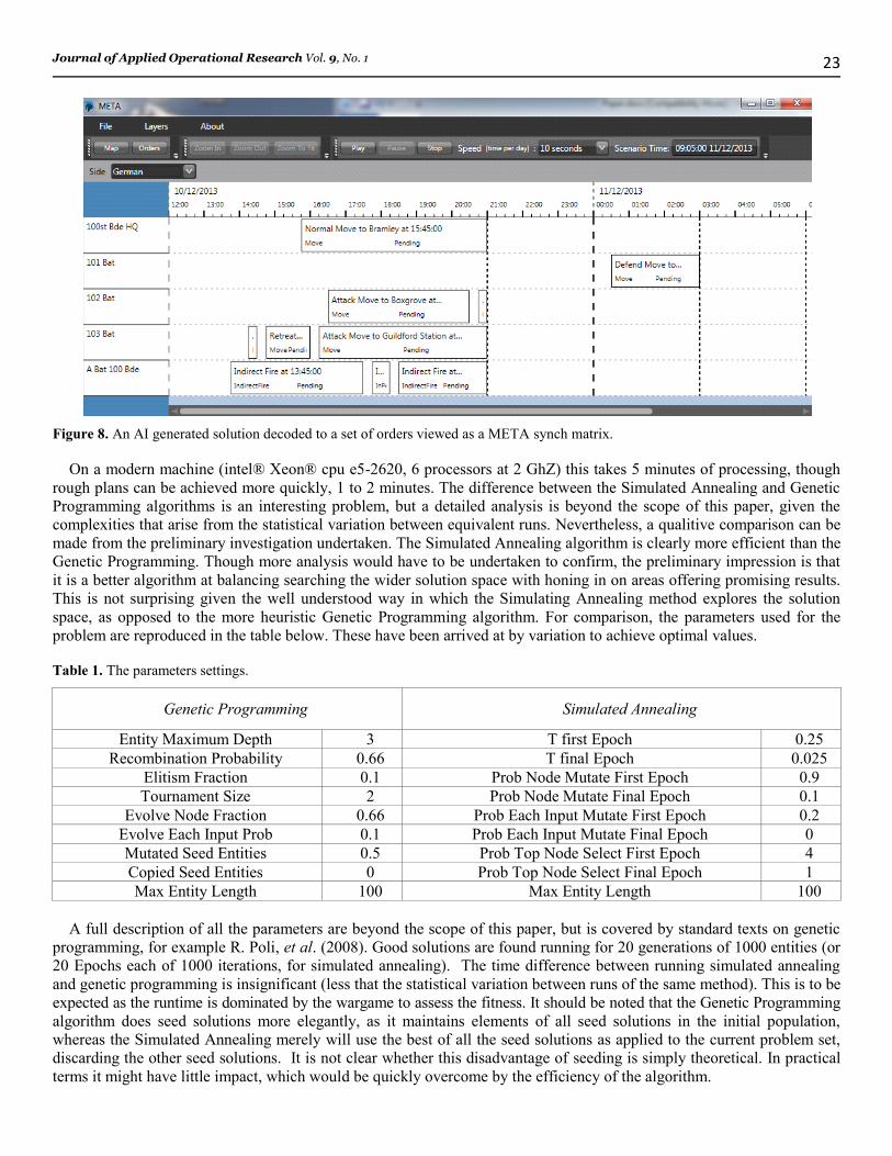
Figure 8. An AI generated solution decoded to a set of orders viewed as a META synch matrix.

On a modern machine (intel® Xeon® cpu e5-2620, 6 processors at 2 GhZ) this takes 5 minutes of processing, though

rough plans can be achieved more quickly, 1 to 2 minutes. The difference between the Simulated Annealing and Genetic

Programming algorithms is an interesting problem, but a detailed analysis is beyond the scope of this paper, given the

complexities that arise from the statistical variation between equivalent runs. Nevertheless, a qualitive comparison can be

made from the preliminary investigation undertaken. The Simulated Annealing algorithm is clearly more efficient than the

Genetic Programming. Though more analysis would have to be undertaken to confirm, the preliminary impression is that

it is a better algorithm at balancing searching the wider solution space with honing in on areas offering promising results.

This is not surprising given the well understood way in which the Simulating Annealing method explores the solution

space, as opposed to the more heuristic Genetic Programming algorithm. For comparison, the parameters used for the

problem are reproduced in the table below. These have been arrived at by variation to achieve optimal values.

Table 1. The parameters settings.

Genetic Programming Simulated Annealing

Entity Maximum Depth 3 T first Epoch 0.25 Recombination Probability 0.66 T final Epoch 0.025

Elitism Fraction 0.1 Prob Node Mutate First Epoch 0.9 Tournament Size 2 Prob Node Mutate Final Epoch 0.1

Evolve Node Fraction 0.66 Prob Each Input Mutate First Epoch 0.2 Evolve Each Input Prob 0.1 Prob Each Input Mutate Final Epoch 0 Mutated Seed Entities 0.5 Prob Top Node Select First Epoch 4 Copied Seed Entities 0 Prob Top Node Select Final Epoch 1 Max Entity Length 100 Max Entity Length 100

A full description of all the parameters are beyond the scope of this paper, but is covered by standard texts on genetic

programming, for example R. Poli, et al. (2008). Good solutions are found running for 20 generations of 1000 entities (or

20 Epochs each of 1000 iterations, for simulated annealing). The time difference between running simulated annealing

and genetic programming is insignificant (less that the statistical variation between runs of the same method). This is to be

expected as the runtime is dominated by the wargame to assess the fitness. It should be noted that the Genetic Programming

algorithm does seed solutions more elegantly, as it maintains elements of all seed solutions in the initial population,

whereas the Simulated Annealing merely will use the best of all the seed solutions as applied to the current problem set,

discarding the other seed solutions. It is not clear whether this disadvantage of seeding is simply theoretical. In practical

terms it might have little impact, which would be quickly overcome by the efficiency of the algorithm.


24

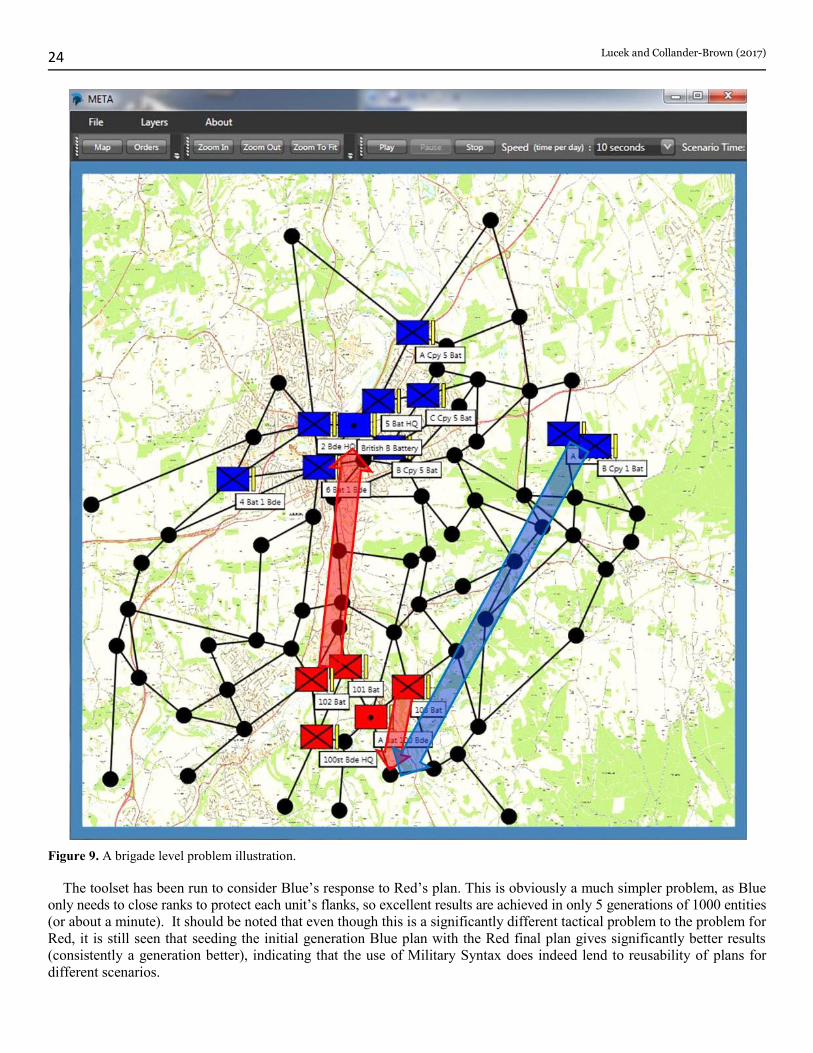
Figure 9. A brigade level problem illustration.

The toolset has been run to consider Blue’s response to Red’s plan. This is obviously a much simpler problem, as Blue

only needs to close ranks to protect each unit’s flanks, so excellent results are achieved in only 5 generations of 1000 entities

(or about a minute). It should be noted that even though this is a significantly different tactical problem to the problem for

Red, it is still seen that seeding the initial generation Blue plan with the Red final plan gives significantly better results

(consistently a generation better), indicating that the use of Military Syntax does indeed lend to reusability of plans for

different scenarios.


25

It is also important to note that even though Blue defending is a problem of significant different complexity to Red

attacking, the careful and robust normalisation of the solution fitness measurement means that the same temperature

profile proves to be optimal when using the simulated annealing method. Indeed, results that seem convincing to the analyst

in both scenarios have very similar fitness measurements, achieving about 80/100 marks, demonstrating the success of the

normalisation of solution fitness.

Conclusions

It has been demonstrated that AI algorithms, such as Simulated Annealing and Genetic Programming can efficiently generate

plans for tactical problems, in this case a brigade level land engagement, generating plans that resemble human decision

making. Two elements have been key to this success. The first is the use of military-like syntax in formulating the solutions

the algorithms work with. This naturally forces the plans into a human-like form and also increases the efficiency in

generating tactically sound plans that need minimal changes when applied to new scenarios. Secondly is that, utilising the

generic nature of the AI algorithms, the toolset has been able to employ a “plug-and-play” architecture. This enables the

use of a meta model that allows the AI to generate plans against a reduced problem set which represents only the essential

elements of the full problem. The solution generated can then be assessed against the full problem (for example SimBrig).

This approach allows the meta model to be simple, fast and robust, overcoming the traditional limitations of the AI techniques

employed, which require the evaluation of many plans and also have a tendency to exploit loopholes in the logic of the

evaluation models.

The META model has also demonstrated a successful approach to wargame simulation. Concentrating on modelling

only what is required for the problem considered, to a suitable level of detail, has enabled building a comprehensive and

credible simulation of brigade level land engagements from scratch, achieved on a limited budget and timescale. The Mission

Planner will allow an exploration of a larger area of the potential solution space than can be explored by human scripting

of behaviour. In particular, it will allow for a wider range of possible Red reactions for particular courses of action and

improve understanding of the value of information. Given the AI is able to generate sound plans for brigade level problems

in the order of a few minutes (using standard specification PCs or laptops), the next step is to imbed the Mission Planner

within a model to test its ability to plan in a dynamic situation.

References

Y. Azaria and M. Sipper (2005). GP-gammon: Genetically programming backgammon players. Genetic Programming and

Evolvable Machines, 6(3):283–300.

Y. Azaria and M. Sipper (2005). Using GP-gammon: Using genetic programming to evolve backgammon players. In M.

Keijzer, et al., editors, Proceedings of the 8th European Conference on Genetic Programming, volume 3447 of Lecture

Notes in Computer Science, pages 132–142, Lausanne, Switzerland, 30 March - 1 April 2005b. Springer.

N.A. Barricelli (1963). "Numerical testing of evolution theories. Part II. Preliminary tests of performance, symbiogenesis

and terrestrial life". Acta Biotheoretica (16): 99–126.

British Army Battle Box, British Army, AC 71632, Edition 13, Army Publications, Army Media & Comm, IDL 407,

Ground Floor, Zone 2, Ramillies Building, Marlborough Lines, Andover, SP11 8HJ,

http://www.baebb.dii.r.mil.uk/baebb/

V. Černý (1985). "Thermodynamical approach to the traveling salesman problem: An efficient simulation algorithm".

Journal of Optimization Theory and Applications 45: 41–51.

A. Fraser, D. Burnell (1970). Computer Models in Genetics. New York: McGraw-Hill.

A. Hauptman and M. Sipper (2005). GP-endchess: Using genetic programming to evolve chess endgame players. In M.

Keijzer, et al., editors, Proceedings of the 8th European Conference on Genetic Programming, volume 3447 of Lecture

Notes in Computer Science, pages 120–131, Lausanne, Switzerland, 30 March - 1 April 2005. Springer.

A. Hauptman and M. Sipper (2007). Evolution of an efficient search algorithm for the mate-in-N problem in chess. In M.

Ebner, et al., editors, Proceedings of the 10th European Conference on Genetic Programming, volume 4445 of Lecture

Notes in Computer Science, pages 78–89, Valencia, Spain, 11 - 13 April 2007. Springer.


26

D. Jackson (2005). Evolving defence strategies by genetic programming, In M. Keijzer, et al., editors, Proceedings of the

8th European Conference on Genetic Programming, volume 3447 of Lecture Notes in Computer Science, pp 281-290,

Lausanne, Switzerland, 30 March - 1 April 2005. Springer.

J. Lohn, G. Hornby, and D. Linden (2004). Evolutionary antenna design for a NASA spacecraft. In U.-M. O’Reilly, et al.,

editors, Genetic Programming Theory and Practice II, chapter 18, pages 301–315. Springer, Ann Arbor, 13-15.

J. R. Koza (1992). Genetic Programming: On the Programming of Computers by Means of Natural Selection. MIT Press,

Cambridge, MA, USA, 1992.

J. R. Koza, F. H. Bennett, III, and O. Stiffelman (1999). Genetic programming as a Darwinian invention machine. In R.

Poli, et al., editors, Genetic Programming, Proceedings of EuroGP’99, volume 1598 of LNCS, pp 93–108, Goteborg,

Sweden, 26-27 May 1999. Springer-Verlag.

F. W. Lanchester (1916). Aircraft in Warfare: The Dawn of the Fourth Arm. London: Constable and Company.

S. Luke (1998). Evolving soccerbots: A retrospective. In Proceedings of the 12th Annual Conference of the Japanese

Society for Artificial Intelligence, 1998. (The simulation of teams of softbot programs in simulated soccer matches)

N. Metropolis, et al. (1953). "Equation of State Calculations by Fast Computing Machines". The Journal of Chemical

Physics 21 (6): 1087

PJHQ J5OA handy OA Guide, undated note, PJHQ

R. Poli, W. B. Langdon, and N. F. McPhee. A field guide to genetic programming (2008). Published via http://lulu.com

and freely available at http://www.gp-field-guide.org.uk, 2008. (With contributions by J. R. Koza)

W.H. Press, S.A. Teukolsky, W.T. Vetterling, B.P. Flannery (2007). "Section 10.12. Simulated Annealing Methods".

Numerical Recipes: The Art of Scientific Computing (3rd ed.). New York: Cambridge University Press.

H. Robbins and S. Monro (1951). "A Stochastic Approximation Method". Annals of Mathematical Statistics 22(3): 400–407.

D Rowland (2006). The Stress of Battle, Quantifying Human Performance in Combat, The Stationary Office.

Y. Shichel, E. Ziserman, and M. Sipper (2005). GP-robocode: Using genetic programming to evolve robocode players. In

M. Keijzer, et al., editors, Proceedings of the 8th European Conference on Genetic Programming, volume 3447 of

Lecture Notes in Computer Science, pages 143–154, Lausanne, Switzerland, 30 March - 1 April 2005. Springer.

J. C. Spall (2003). Introduction to Stochastic Search and Optimization. Wiley.

Zhao Le, et al. (2014). Optimizing the train timetable for a subway system, Proceedings of the Institution of Mechanical

Engineers, Part F: Journal of Rail and Rapid Transit, 13 March 2014.

Documents

Using artificial intelligence algorithms for high level ...orlabanalytics.ca/jaor/archive/v9/n1/jaorv9n1p11.pdf · Using artificial intelligence algorithms for high level tactical