N92-19740

USER'S MANUAL FOR

THREE DIMENSIONAL FDTD

VERSION D CODE FOR SCATTERING

FROM FREQUENCY-DEPENDENT DIELECTRIC

AND MAGNETIC MATERIALS

by

John H. Beggs, Raymond J. Luebbers and Karl S. Kunz

Electrical and Computer Engineering Department

The Pennsylvania State University

University Park, PA 16802

(814) 865-2362

January 1992

https://ntrs.nasa.gov/search.jsp?R=19920010498 2018-06-04T04:59:41+00:00Z

I •

II.

III.

IV.

V.

VI.

VII.

VIII.

IX.

X.

XI.

XII.

TABLE OF CONTENTS

INTRODUCTION .....................

FDTD METHOD .....................

OPERATION .......................

RESOURCE REQUIREMENTS ................

VERSION D CODE CAPABILITIES ...............

DEFAULT SCATTERING GEOMETRY ..............

SUBROUTINE DESCRIPTION ................

MAIN ROUTINE ......................

SUBROUTINE SETFZ ...................

SUBROUTINE SAVFZ ...................

SUBROUTINE FAROUT ..................

SUBROUTINE BUILD ...................

SUBROUTINE DCUBE ...................

SUBROUTINE SETUP ...................

SUBROUTINE EXSFLD .................

SUBROUTINE EYSFLD ..................

SUBROUTINE EZSFLD .................

SUBROUTINES RADEYX, RADEZX, RADEZY, RADEXY, RADEXZ and

RADEYZ .....................

SUBROUTINE HXSFLD .................

SUBROUTINE HYSFLD .................

SUBROUTINE HZSFLD ..................

SUBROUTINES RADHXZ, RADHYX, RADHZY, RADHXY, RADHYZ and

RADHZX .....................

SUBROUTINE DATSAV "EZI; HXi,'HYI'and'HZI" [ [ [ [ [ [FUNCTIONS EXI, EYI,

FUNCTION SOURCE ..................

FUNCTIONS DEXI, DEYI, DEZI, DHXI, DHYI and DHZI • •

FUNCTIONS DEXIXE, DEYIXE, DEZIXE, DHXIXE, DHYIXE and

DHZIXE .....................

FUNCTION DSRCE ..................

FUNCTION DCONV ....................

SUBROUTINE ZERO ...................

INCLUDE FILE DESCRIPTION (COMMOND.FOR) .......

RCS COMPUTATIONS ...................

RESULTS ......................

SAMPLE PROBLEM SETUP ................

NEW PROBLEM CHECKLIST ................

COMMOND.FOR ....................

5

7

8

8

9

9

i0

i0

i0

i0

ii

14

15

15

16

16

16

16

16

16

16

17

17

17

17

17

18

18

18

19

19

20

20

22

XIII.

XI.

TABLE OF CONTENTS (cont.)

SUBROUTINE BUILD ...................

SUBROUTINE SETUP ...................

FUNCTIONS SOURCE and DSRCE .............

SUBROUTINE DATSAV ..................

REFERENCES .....................

FIGURE TITLES ....................

22

22

23

23

23

23

I. INTRODUCTION

The Penn State Finite Difference Time Domain Electromagnetic

Scattering Code Version D is a three dimensional numerical

electromagnetic scattering code based upon the Finite Difference

Time Domain Technique (FDTD). The supplied version of the code

is one version of our current three dimensional FDTD code set.

This manual provides a description of the code and corresponding

results for several scattering problems. The manual is organized

into fourteen sections: introduction, description of the FDTD

method, operation, resource requirements, Version D code

capabilities, a brief description of the default scattering

geometry, a brief description of each subroutine, a description

of the include file (COMMOND.FOR), a section briefly discussing

Radar Cross Section (RCS) computations, a section discussing some

scattering results, a sample problem setup section, a new problem

checklist, references and figure titles.

II. FDTD METHOD

The Finite Difference Time Domain (FDTD) technique models

transient electromagnetic scattering and interactions with

objects of arbitrary shape and/or material composition. The

technique was first proposed by Yee [i] for isotropic, non-

dispersive materials in 1966; and has matured within the past

twenty years into a robust and efficient computational method.

The present FDTD technique is capabable of transient

electromagnetic interactions with objects of arbitrary and

complicated geometrical shape and material composition over a

large band of frequencies. This technique has recently been

extended to include dispersive dielectric materials, chiral

materials and plasmas.

In the FDTD method, Maxwell's curl equations are discretized

in time and space and all derivatives (temporal and spatial) are

approximated by central differences. The electric and magnetic

fields are interleaved in space and time and are updated in a

second-order accurate leapfrog scheme. The computational space

is divided into cells with the electric fields located on the

edges and the magnetic fields on the faces (see Figure i). FDTD

objects are defined by specifying dielectric and/or magnetic

material parameters at electric and/or magnetic field locations.

Two basic implementations of the FDTD method are widely used

for electromagnetic analysis: total field formalism and scattered

field formalism. In the total field formalism, the electric and

magnetic field are updated based upon the material type present

at each spatial location. In the scattered field formalism, the

incident waveform is defined analytically and the scattered field

is coupled to the incident field through the different material

types. For the incident field, any waveform, angle of incidence

and polarization is possible. The separation of the incident and

5

scattered fields conveniently allows an absorbing boundary to beemployed at the extremities of the discretized problem space toabsorb the scattered fields.

This code is a scattered field code, and the total E and Hfields may be found by combining the incident and scatteredfields. Any type of field quantity (incident, scattered, ortotal), Poynting vector or current are available anywhere within

the computational space. These fields, incident, scattered and

total, may be found within, on or about the interaction object

placed in the problem space. By using a near to far field

transformation, far fields can be determined from the near fields

within the problem space thereby affording radiation patterns and

RCS values. The accuracy of these calculations is typically

within a dB of analytic solutions for dielectric and magnetic

sphere scattering. Further improvements are expected as better

absorbing boundary conditions are developed and incorporated.

III. OPERATION

Typically, a truncated Gaussian incident waveform is used to

excite the system being modeled, however certain code versions

also provide a smooth cosine waveform for convenience in modeling

dispersive materials. The interaction object is defined in the

discretized problem space with arrays at each cell location

created by the discretization. All three dielectric material

types for E field components within a cell can be individually

specified by the arrays IDONE(I,J,K), IDTWO(I,J,K),

IDTHRE(I,J,K). This models arbitrary dielectric materials with

= _0- By an obvious extension to six arrays, magnetic materials

with _ _ _0 can be modeled.

Scattering occurs when the incident wave, marched forward in

time in small steps set by the Courant stability condition,

reaches the interaction object. Here a scattered wave must

appear along with the incident wave so that the Maxwell equations

are satisfied. If the material is a perfectly conductive metal

then only the well known boundary condition

scat incEtan = _Etan (1)

must be satisfied. For a nondispersive dielectric the

requirement is that the total field must satisfy the Maxwell

equations in the material:

_7×E t°t = V×(E inc+E scat ) =1 aH t°t 1 a(HinC+H scat )

_o at _o at

(2)

6

V×H t°t --V× (Hinc +H scat) =_dE tot

+ aE t°tat

(3)

a (Einc + E scat ) EinC + Escat=e +o( )at

(4)

Additionally the incident wave, defined as moving unimpeded

through a vacuum in the problem space, satisfies everywhere in

the problem the Maxwell equations for free space

VX E inc= 1 @H inc

Po at

(5)

aE inc

_7x Hinc =eo--at

(6)

Subtracting the second set of equations from the first yields the

Maxwell equations governing the scattered fields in the material:

1 aH scatVx E scat = ( 7 )

/1'o at

VxH scat = (8 -go)

aE inc . aE scat+GE lnc+¢_ +GE scat

at at(8)

Outside the material this simplifies to:

I aH scatVx Escat= (9 )

Po at

a E scatVxHsCat =¢ (10)

o- at

Magnetic materials, dispersive effects, non-linearities,

etc., are further generalizations of the above approach. Based

on the value of the material type, the subroutines for

calculating scattered E and H field components branch to the

appropriate expression for that scattered field component and

that component is advanced in time according to the selectedalgorithm. As many materials can be modeled as desired, thenumber equals the dimension selected for the flags. If materialswith behavior different from those described above must bemodeled, then after the appropriate algorithm is found, thecode's branching structure allows easy incorporation of the newbehavior.

IV. RESOURCE REQUIREMENTS

The number of cells the problem space is divided into times

the six components per cell set the problem space storage

requirements

Storage=NC x 6 components/cell x 4 bytes/component (ii)

and the computational cost

Operations=NC x 6 comp/cell x i0 ops/component × N (12)

where N is the number of time steps desired.

N typically is on the order of ten times the number of cells

on one side of the problem space. More precisely for cubical

cells it takes _ time steps to traverse a single cell when the

time step is set by the Courant stability condition

AxAt- _x = cell size dimension (13)

The condition on N is then that

I I

N - 10x(_NC _) NC _ ~ number cells on a side (14)of the problem space

The earliest aircraft modeling using FDTD with approximately 30

cells on a side required approximately 500 time steps. For more

recent modeling with approximately i00 cells on a side, 2000 or

more time steps are used.

For (I00 cell) 3 problem spaces, 24 MBytes of memory are

required to store the fields. Problems on the order of this size

have been run on a Silicon Graphics 4D 220 with 32 MBytes of

memory, IBM RISC 6000, an Intel 486 based machine, and VAX

11/785. Storage is only a problem as in the case of the 486

where only 16 MBytes of memory was available. 3This limited the

problem space size to approximately (80 cells) .

For (i00 cell) 3 problem_ with approximately 2000 time steps,there is a total of 120 x i_ operations to perform. The speedsof the previously mentioned machines are 24 MFLOPs (4 processorupgraded version), i0 MFLQPS, 1.5 MFLOPS, _nd 0.2 MFLOPs. T_erun times are then 53x i0_ seconds, 12 x i0 seconds, 80 x I0seconds and 600 x i0 seconds, respectively. In hours the timesare 1.4, 3.3, 22.2 and 167 hours. Problems of this size arepossible on all but the last machine and can in fact be performedon a personal computer (486) if one day turnarounds arepermissible.

V. VERSION D CODE CAPABILITIES

The Penn State University FDTD Electromagnetic Scattering

Code Version D has the following capabilities:

i) Ability to model lossy dielectric and perfectly conducting

scatterers.

2) Ability to model lossy magnetic scatterers.

3) Ability to model dispersive dielectric and dispersive

magnetic scatterers. This dispersive FDTD method is nowdesignated (FD)-TD for Frequency-Dependent Finite Difference Time

Domain.

4) First and second order outer radiation boundary condition

(ORBC) operating on the electric fields for dielectric and

dispersive dielectric scatterers.

5) First and second order ORBC operating on the magnetic fields

for magnetic and dispersive magnetic scatterers.

6) Near to far zone transformation capability to obtain far zone

scattered fields.

7) Gaussian and smooth cosine incident waveforms with arbitrary

incidence angles.

8) Near zone field, current or power sampling capability.

9) Companion code for computing Radar Cross Section (RCS).

VI. DEFAULT SCATTERING GEOMETRY

The code as delivered is set up to calculate the far zone

backscatter fields for a 6.67 meter radius, dispersive, Nickel

Ferrite sphere. Nickel Ferrite is defined by a frequency

dependent permeability given by

where _® is the infinite frequency permeability, _s is the zero

-p,® +_0 I+J_T0

(15)

frequency permeability, TO is the relaxation time and _ is the

radian frequency. The Nickel Ferrite parameters are _®=i, _s=lO0

and T0=20 ns. The problem space size is 66 by 66 by 66 cells in

the x, y and z directions, the cells are 1/3 m cubes, and the

incident waveform is a 0-polarized smooth cosine pulse with

incidence angles of 8=22.5 and 0=22.5 degrees. The output data

files are included as a reference along with a code (RCS3D.FOR)

for computing the frequency domain RCS using these output data

files. The ORBC is the second order absorbing boundary condition

set forth by Mur [2].

VII. SUBROUTINE DESCRIPTION

In the description for each subroutine, an asterisk (*) will

be placed by the subroutine name if that particular subroutine is

normally modified when defining a scattering problem.

MAIN ROUTINE

The main routine in the program contains the calls for all

necessary subroutines to initialize the problem space and

scattering object(s) and for the incident waveform, far zone

transformation, field update subroutines, outer radiation

boundary conditions and field sampling.

The main routine begins with the include statement and then

appropriate data files are opened, and subroutines ZERO, BUILD

and SETUP are called to initialize variables and/or arrays, build

the object(s) and initialize the incident waveform and

miscellaneous parameters, respectively. Subroutine SETFZ is

called to intialize parameters for the near to far zone

transformation if far zone fields are desired.

The main loop is entered next, where all of the primary

field computations and data saving takes place. During each time

step cycle, the EXSFLD, EYSFLD, and EZSFLD subroutines are called

to update the x, y, and z components of the scattered electric

field. The six electric field outer radiation boundary

conditions (RADE??) are called next to absorb any outgoing

scattered fields for perfectly conducting, dielectric, or

dispersive dielectric scatterers. Time is then advanced 1/2 time

step according to the Yee algorithm and then the HXSFLD, HYSFLD,

AND HZSFLD subroutines are called to update the x, y, and z

components of scattered magnetic field. The six magnetic field

i0

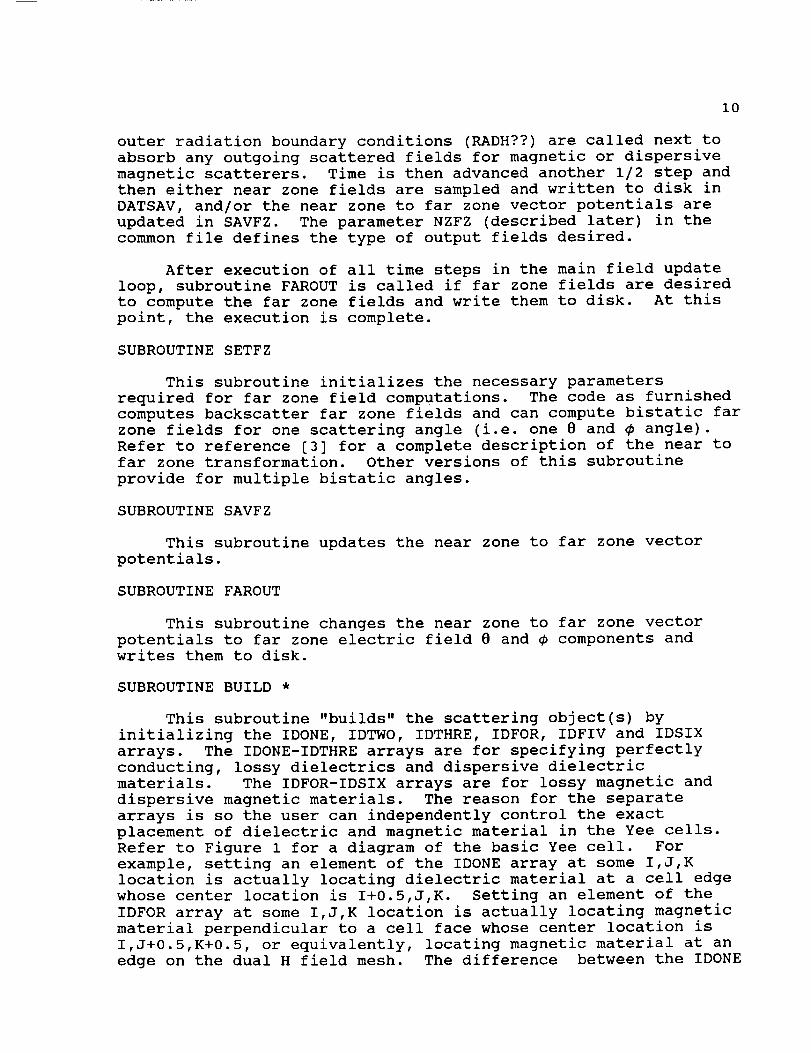
outer radiation boundary conditions (RADH??) are called next toabsorb any outgoing scattered fields for magnetic or dispersivemagnetic scatterers. Time is then advanced another 1/2 step andthen either near zone fields are sampled and written to disk inDATSAV, and/or the near zone to far zone vector potentials areupdated in SAVFZ. The parameter NZFZ (described later) in thecommon file defines the type of output fields desired.

After execution of all time steps in the main field updateloop, subroutine FAROUTis called if far zone fields are desiredto compute the far zone fields and write them to disk. At thispoint, the execution is complete.

SUBROUTINESETFZ

This subroutine initializes the necessary parametersrequired for far zone field computations. The code as furnishedcomputes backscatter far zone fields and can compute bistatic farzone fields for one scattering angle (i.e. one 8 and _ angle).Refer to reference [3] for a complete description of the near tofar zone transformation. Other versions of this subroutineprovide for multiple bistatic angles.

SUBROUTINESAVFZ

This subroutine updates the near zone to far zone vectorpotentials.

SUBROUTINEFAROUT

This subroutine changes the near zone to far zone vectorpotentials to far zone electric field 8 and _ components andwrites them to disk.

SUBROUTINEBUILD *

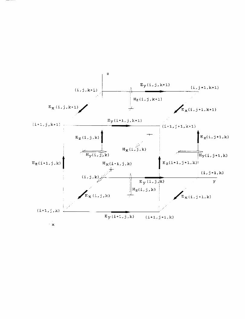
This subroutine "builds" the scattering object(s) byinitializing the IDONE, IDTWO, IDTHRE, IDFOR, IDFIV and IDSIXarrays. The IDONE-IDTHRE arrays are for specifying perfectlyconducting, lossy dielectrics and dispersive dielectricmaterials. The IDFOR-IDSIX arrays are for lossy magnetic anddispersive magnetic materials. The reason for the separatearrays is so the user can independently control the exactplacement of dielectric and magnetic material in the Yee cells.Refer to Figure 1 for a diagram of the basic Yee cell. Forexample, setting an element of the IDONE array at some I,J,Klocation is actually locating dielectric material at a cell edgewhose center location is I+0.5,J,K. Setting an element of theIDFOR array at some I,J,K location is actually locating magneticmaterial perpendicular to a cell face whose center location isI,J+0.5,K+0.5, or equivalently, locating magnetic material at anedge on the dual H field mesh. The difference between the IDONE

ii

and IDFOR array locations is a direct result of the field offsetsin the Yee cell (see Figure i). Thus, materials with diagonalpermittivity and/or diagonal permeability tensors can be modeled.The default material type for all ID??? arrays is 0, or freespace. By initializing these arrays to values other than 0, theuser is defining an object by determining what material types arepresent at each spatial location. Other material types availablefor IDONE-IDTHRE are 1 for perfectly conducting objects, 2-9 forlossy non-magnetic dielectrics, 20-29 for dispersive dielectrics.IDONE-IDTHRE are normally set to 0 for magnetic scatterers. Othermaterial types available for IDFOR-IDSIX are 10-19 for lossymagnetic materials and 30-39 for dispersive magnetic materials.IDFOR-IDSIX are normally set to 0 for perfectly conducting ordielectric scatterers. If the user wants a material with bothdielectric and magnetic properties (i.e. permittivity other thane0 for magnetic materials, and permeability other than _0 fordielectric materials), then he/she must define IDONE-IDSIX forthat particular material. This subroutine also has a sectionthat checks the ID??? arrays to determine if legal material typeshave been defined throughout the problem space# The actual non-dispersive material parameters (_, _, a, and a ) are defined in

subroutine SETUP. The dispersive material parameters (Es, e®,

To, a, _s, _®, r0, and a ) are also defined in a separate section

in SETUP. The default geometry is a 6.67 m radius, dispersive,

Nickel Ferrite sphere.

The user must be careful that his/her object created in the

BUILD subroutine is properly formed. There is not a direct

one-to-one correspondence between the dielectric and magnetic

ID??? arrays. However, one can define a correspondence, so that

code used to generate a dielectric object can be modified to

generate a magnetic object.

To see this consider that we have set the permittivity at

cell locations corresponding to

EX(I,J,K), EY(I,J,K), EZ(I,J,K)

using the IDONE, IDTWO, and IDTHRE arrays respectively. This

determines one corner of a dielectric cube. If we wish to define

the corner of a corresponding magnetic cube, offset 1/2 cell in

the x, y, z directions, we would set the locations of the

magnetic fields

HX(I+I,J,K), HY(I,J+I,K), HZ(I,J,K+I)

as magnetic material using the IDFOR, IDFIV, and IDSIX arrays.

This example indicates the following correspondence between

BUILDing dielectric and magnetic objects:

12

Dielectric MagneticObject Object

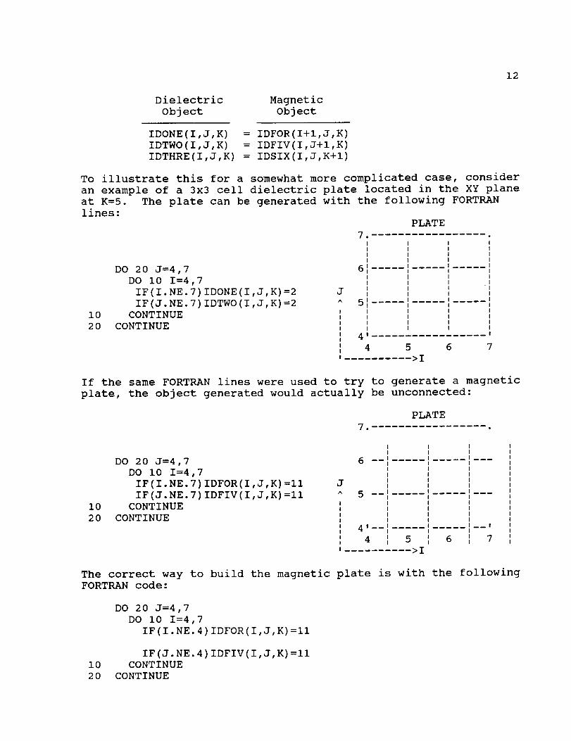
IDONE(I,J,K) = IDFOR(I+I,J,K)IDTWO(I,J,K) = IDFIV(I,J+I,K)IDTHRE(I,J,K) = IDSIX(I,J,K+I)

To illustrate this for a somewhat more complicated case, consideran example of a 3x3 cell dielectric plate located in the XY planeat K=5. The plate can be generated with the following FORTRANlines:

PLATE

i020

DO 20 J=4,7DO i0 I=4,7

IF(I. NE. 7) IDONE(I,J,K) =2IF(J.NE. 7) IDTWO(I,J,K) =2

CONTINUECONTINUE

JA

6

5

4

4 5 6 7

.......... >I

If the same FORTRAN lines were used to try to generate a magnetic

plate, the object generated would actually be unconnected:

,

PLATE

i0

20

DO 20 J=4,7

DO i0 I=4,7

IF (I.NE. 7) IDFOR (I, J,K)=ii

IF (J.NE. 7) IDFIV (I, J,K)=ii

CONTINUE

CONTINUE

JA

_m

5 ----

4t----

4 5

.......... >I

6 7

The correct way to build the magnetic plate is with the following

FORTRAN code:

DO 20 J=4,7

DO i0 I=4,7

IF(I.NE.4)IDFOR(I,J,K)=II

IF(J. NE. 4) IDFIV(I,J,K) =ii

i0 CONTINUE

20 CONTINUE

13

This is equivalent to the correspondence relationship givenabove. See comments in the BUILD subroutine for furtherexplanation of the ID??? arrays.

When it is important to place the object in the center ofthe problem space (to have lowest possible cross-pol scatteringfor symmetric objects), NX etc. should be odd for dielectrics andeven for magnetics. This is due to the field locations in theYee cell and also the placement of the E and H field absorbingboundary condition surfaces.

If the object being modeled has curved surfaces, edges, etc.that are at an angle to one or more of the coordinate axes, thenthat shape must be approximately modeled by lines and faces in a"stair-stepped" (or stair-cased) fashion. This stair-casedapproximation introduces errors into computations at higherfrequencies. Intuitively, the error becomes smaller as morecells are used to stair-case a particular object. Thus, thedefault Nickel Ferrite sphere scattering geometry is a stair-cased sphere.

When the user's test object is dielectric it is apparentlybetter to use the Mur E field boundary formulation. For amagnetic scattering object it seems better to use the Mur H fieldboundary formulation. The reason for this has to do with thereactive part of the energy (near zone fields) reaching theabsorbing boundary surface. These near zone fields differ formagnetic and dielectric objects, even for dual objects where thefar fields are essentially identical.

One final comment on building dual dielectric vs magneticobjects can be explained by considering the duality betweenmagnetic and dielectric materials. In testing the code, it washelpful to test dual dielectric/magnetic objects since theyscatter identically in the far zone. In specifying the materialof a magnetic scatterer to be the dual of a dielectric, thefollowing transformation must be applied:

DIELECTRIC <--DUAL--> MAGNETIC

E fieldH field

E

S (k)

a

< ........ > H field

< ........ > -E field

< ........ >< ........ > E

< ........ > _ (k)< ........ > c;.(P,olEo)=(_

The somewhat surprising entry in this table is the relationship

between the dielectric and magnetic conductivities. The reason

why the magnetic conductivity, a , for magnetic materials has to

be scaled as indicated is that for duality to be applied the free

14

space impedance must be inverted. Although this is not generallypossible for actual problems, identical far zone scattering fordielectric and magnetic scatterers can be achieved by thisscaling of a as above and realizing that E and H scattered _ieldto incident field ratios will not invert. This scaling of a iswhy conductivity for magnetic materials is usually not adominating feature, and in fact is often neglected.

SUBROUTINEDCUBE

This subroutine builds cubes of dielectric material bydefining four each of IDONE, IDTWO and IDTHRE componentscorresponding to one spatial cube of dielectric material. It canalso be used to define thin (i.e. up to one cell thick)dielectric or perfectly conducting plates. Refer to commentswithin DCUBE for a description of the arguments and usage of thesubroutine. This subroutine could be modified to build cubesand/or plates of magnetic materials by using a triple do-loop inBUILD (after calls to DCUBE) over coordinate indices I, J, K andapplying the correspondence between the IDONE-IDTHRE and IDFOR-IDSIX arrays that was previously discussed.

SUBROUTINESETUP *

This subroutine initializes many of the constants requiredfor incident field definition, field update equations, outerradiation boundary conditions and, material parameters. Thematerial parameters E, _, a and a are defined for each material

type (non-dispersive) using the material arrays EPS, XMU, SIGMA

and SIGMAC respectively. The array EPS is used for the total

permittivity, XMU is used for the total permeability, SIGMA is

used for the electric conductivity and SIGMAC is used for the

magnetic conductivity (useful for running dual problems). These

arrays are initialized in SETUP to free space material parameters

for all material types and then the user is required to modify

these arrays for his/her scattering materials. Thus, for the

lossy dielectric material type 2, the user must define EPS(2) and

SIGMA (2 ) .

For dispersive dielectric and magnetic materials, different

material parameter arrays are used. The functional form of the

frequency dependent permittivity/permeability that was

implemented in the code is the Debye relaxation [4] with an

effective DC conductivity given by

a

_(_) = E/-jE//= E®E 0 + 60Xe(_))+ -- (16)j_

where the frequency dependent electric susceptibility function is

defined as

15

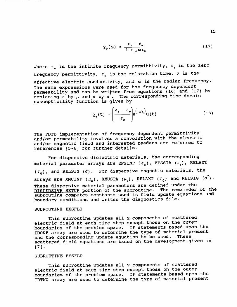
es - e. (17)

where _= is the infinite frequency permittivity, _s is the zero

frequency permittivity, T O is the relaxation time, a is the

effective electric conductivity, and _ is the radian frequency.

The same expressions were used for the frequency dependent

permeability and can be written from equations (16) and (17) by

replacing E by _ and a by a . The corresponding time domain

susceptibility function is given by

- (,i,0)(tlXe(t) = e uTO

(18)

The FDTD implementation of frequency dependent permittivity

and/or permeability involves a convolution with the electric

and/or magnetic field and interested readers are referred to

references [5-6] for further details.

For dispersive dielectric materials, the corresponding

material parameter arrays are EPSINF (E.), EPSSTA (_s), RELAXT

(To) , and RELSIG (a). For dispersive magnetic materials, thet

arrays are XMUINF (_®), XMUSTA (_s), RELAXT (To) and RELSIG (a).

These dispersive material parameters are defined under the

DISPERSIVE SETUP portion of the subroutine. The remainder of the

subroutine computes constants used in field update equations and

boundary conditions and writes the diagnostics file.

SUBROUTINE EXSFLD

This subroutine updates all x components of scattered

electric field at each time step except those on the outer

boundaries of the problem space. IF statements based upon the

IDONE array are used to determine the type of material present

and the corresponding update equation to be used. These

scattered field equations are based on the development given in

[7].

SUBROUTINE EYSFLD

This subroutine updates all y components of scattered

electric field at each time step except those on the outer

boundaries of the problem space. IF statements based upon the

IDTWO array are used to determine the type of material present

16

and the corresponding update equation to be used.

SUBROUTINEEZSFLD

This subroutine updates all z components of scatteredelectric field at each time step except those on the outerboundaries of the problem space. IF statements based upon theIDTHRE array are used to determine the type of material presentand the corresponding update equation to be used.

SUBROUTINESRADEYX, RADEZX, RADEZY, RADEXY, RADEXZ and RADEYZ

These subroutines apply the outer radiation boundaryconditions to the scattered electric field on the outerboundaries of the problem space for non-magnetic scatterers. Theuser controls selection of these routines through the parameterMAGNET(described later).

SUBROUTINEHXSFLD

This subroutine updates all x components of scatteredmagnetic field at each time step. IF statements based upon theIDFOR array are used to determine the type of material presentand the corresponding update equation to be used.

SUBROUTINEHYSFLD

This subroutine updates all y components of scatteredmagnetic field at each time step. IF statements based upon theIDFIV array are used to determine the type of material presentand the corresponding update equation to be used.

SUBROUTINEHZSFLD

This subroutine updates all z components of scatteredmagnetic field at each time step. IF statements based upon theIDSIX array are used to determine the type of material presentand the corresponding update equation to be used.

SUBROUTINESRADHXZ, RADHYX, RADHZY, RADHXY, RADHYZand RADHZX

These subroutines apply the outer radiation boundaryconditions to the scattered magnetic field on the outerboundaries of the problem space for magnetic scatterers. Theuser controls selection of these routines through the parameterMAGNET(described later).

SUBROUTINEDATSAV *

17

This subroutine samples near zone scattered field quantitiesand saves them to disk. This subroutine is where the quantitiesto be sampled and their spatial locations are to be specified andis only called if near zone fields only are desired or if bothnear and far zone fields are desired. Total field quantities canalso be sampled. See comments within the subroutine forspecifying sampled scattered and/or total field quantities. Whensampling magnetic fields, remember the 6t/2 time difference

between E and H when writing the fields to disk. Sections of

code within this subroutine determine if the sampled quantities

and the spatial locations have been properly defined.

FUNCTIONS EXI, EYI, EZI, HXI, HYI and HZI

These functions are called to compute the x, y and z

components of incident electric and magnetic field, respectively.

The functional form of the incident field is contained in a

separate function SOURCE.

FUNCTION SOURCE *

This function contains the functional form of the incident

field. The code as furnished uses the smooth cosine form of the

incident field. An incident Gaussian pulse is also available by

uncommenting the required lines and commenting out the smooth

cosine pulse. Thus, this function need only be modified if the

user changes the incident pulse from smooth cosine to Gaussian.

Currently, onlv the smooth cosine pulse can be used for

scattering from dispersive targets. A slight improvement in

computing speed and vectorization may be achieved by moving this

function inside each of the incident field functions EXI, EYI and

so on.

FUNCTIONS DEXI, DEYI, DEZI, DHXI, DHYI and DHZI

These functions are called to compute the x, y and z

components of the time derivative of incident electric and

magnetic field, respectively. The functional form of the

incident field is contained in a separate function DSRCE.

FUNCTIONS DEXIXE, DEYIXE, DEZIXE, DHXIXE, DHYIXE and DHZIXE

These functions compute the x, y and z components of the

convolution of the time derivative of the incident field with the

electric or magnetic Debye susceptibility function X.

FUNCTION DSRCE *

18

This function contains the functional form of the timederivative of the incident field. The code as furnished uses thetime derivative of the smooth cosine form of the incident field.A Gaussian pulse time derivative is also available byuncommenting the required lines and commenting out the smoothcosine pulse. Thus, the function need only be modified if theuser changes from the smooth cosine to Gaussian pulse. Again, aslight improvement in computing speed and vectorization may beachieved by moving this function inside each of the timederivative incident field functions DEXI, DEYI and so on.

FUNCTION DCONV

This function evaluates the convolution of the timederivative of the incident field with the Debye susceptibilityfunction X-

SUBROUTINE ZERO

This subroutine initializes various arrays and variables tozero.

VIII. INCLUDE FILE DESCRIPTION (COMMOND.FOR) *

The include file, COMMOND.FOR, contains all of the arrays

and variables that are shared among the different subroutines.

This file will require the most modifications when defining

scattering problems. A description of the parameters that are

normally modified follows.

The parameters NX, NY and NZ specify the size of the problem

space in cells in the x, y and z directions respectively. For

problems where it is crucial to center the object within the

problem space, then NX, NY and NZ should be odd for dielectric

scatterers and even for magnetic scatterers. The parameter NTEST

defines the number of near zone quantities to be sampled and NZFZ

defines the field output format. Set NZFZ=O for near zone fields

only, NZFZ=I for far zone fields only and NZFZ=2 for both nearand far zone fields. Parameter MAGNET is used to define magnetic

scatterers and it controls the choice of RADE?? versus RADH??

absorbing boundary subroutines. It is set to 0 for dielectric

scatterers and to 1 for magnetic scatterers. Parameter NUMMAT

defines the total number of material types that are available for

use. NEDISP and NHDISP define the number of dispersive

dielectric and magnetic materials that are being used. Parameter

NSTOP defines the maximum number of time steps. DELX, DELY, and

DELZ (in meters) define the cell size in the x, y and z

directions respectively. The 8 and _ incidence angles (in

degrees) are defined by THINC and PHINC respectively and the

polarization is defined by ETHINC and EPHINC. ETHINC=I.0,

EPHINC=0.0 for 8-polarized incident field and ETHINC=O.0,

19

EPHINC=I.0 for _-polarized incident fields. 2 Parameters AMP andBETA define the maximum amplitude and the e temporal width ofthe incident pulse respectively. BETA automatically adjusts whenthe cell size is changed and normally should not be changed bythe user. The far zone scattering angles are defined by THETFZand PHIFZ. The code as furnished performs backscattercomputations, but these parameters could be modified for abistatic computation.

IX. RCS COMPUTATIONS

A companion code, RCS3D.FOR, has been included to cgmpute

RCS versus frequency. It uses the file name of the (FD)_TD far

zone output data (FZOUT3D.DAT) and writes data files of far zone

electric fields versus time (FZTIME.DAT) and RCS versus frequency

(3DRCS.DAT). The RCS computations are performed up to the i0

cell/l 0 frequency limit. Refer to comments within this code forfurther details.

X. RESULTS

As previously mentioned, the code as furnished models a 6.67

m radius, dispersive, Nickel Ferrite sphere and computes

backscatter far zone scattered fields at angles of 8=22.5 and

_=22.5 degrees. Results are included for 0.25 dB loaded

dielectric and magnetic foam spheres, 60 dB dielectric and

magnetic foam spheres and the Nickel Ferrite magnetic sphere.

The material parameters for 0.25 dB and 60 dB loaded foam are:

0.25 DB FOAM 60 DB FOAM

1.16 E s 41.0

1.01 E® 1.6

0.6497 ns TO 0.3450 ns

2.954E-04 S/m u 3.902E-01 S/m

The magnetic materials are duals of the above as described

earlier with the relative conductivity scaled by the ratio _0/_0.

The Nickel Ferrite parameters are _®=i, _s=100, T0=20 ns and

a =0.0. For the 0.25 dB foams there are i0 cells per wavelength

at approximately 3.0 GHz. For the 60 dB foam there are i0 cells

per wavelength at approximately 2.35 GHz, as the 60 dB foam has a

higher dielectric constant.

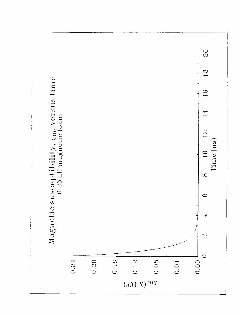
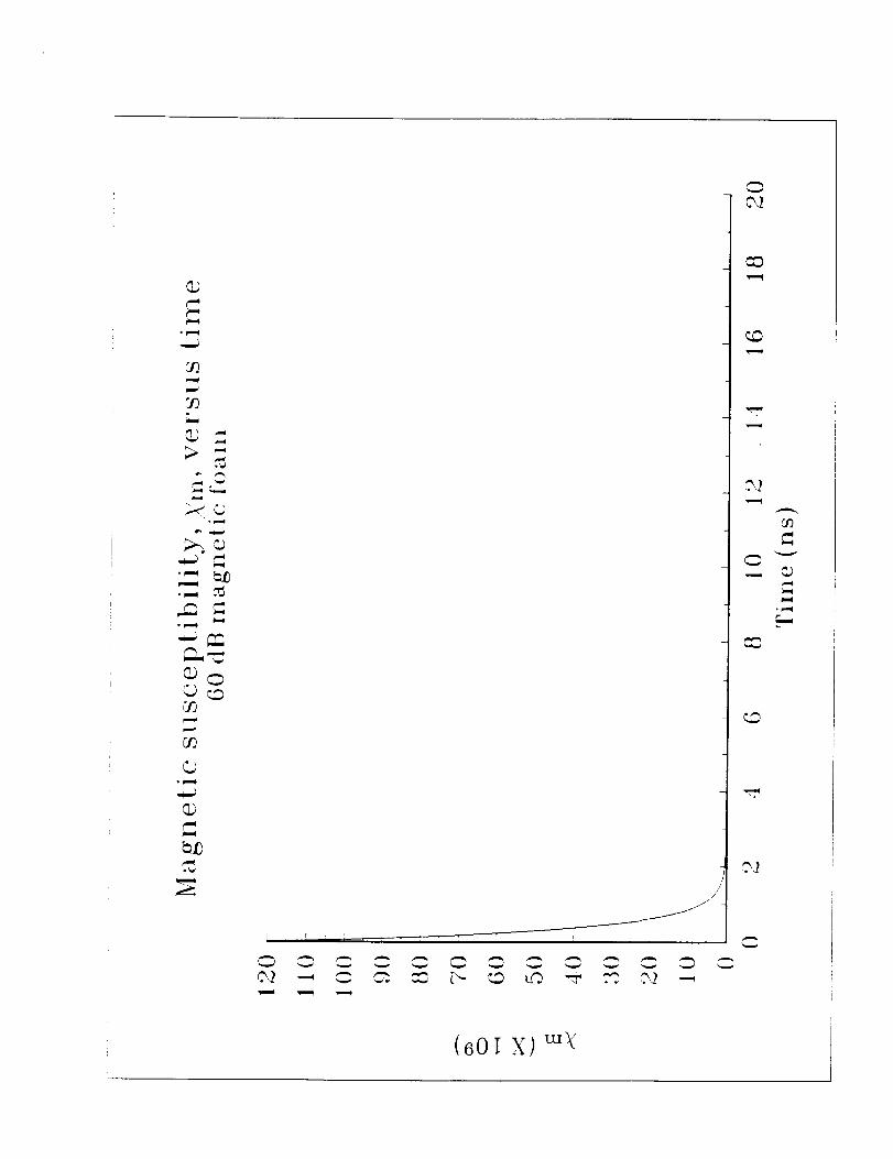
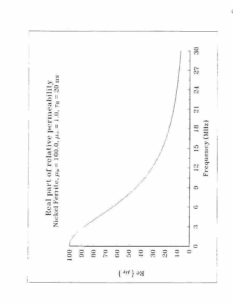
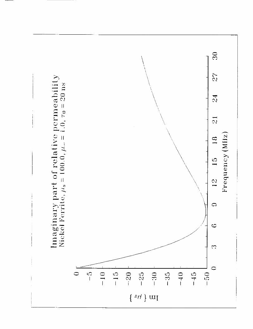
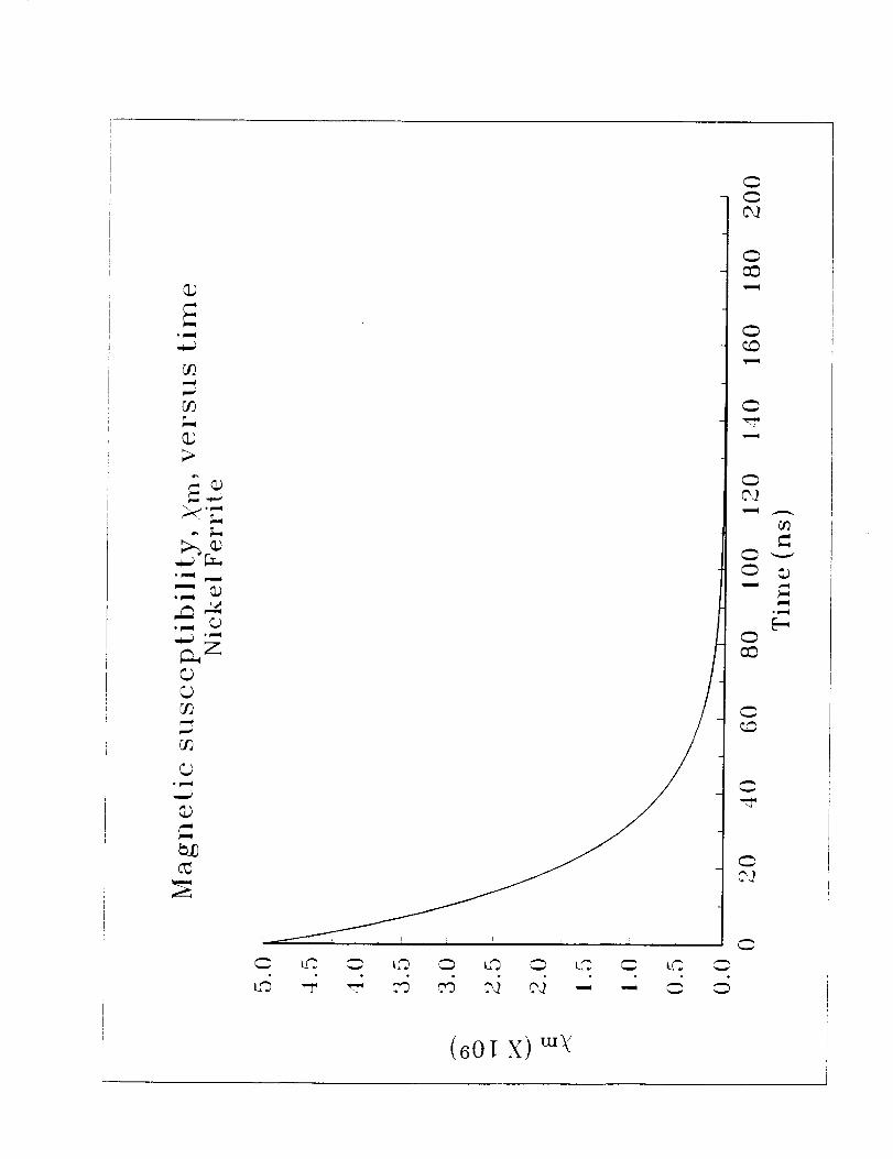
Figures 2-10 show the real and imaginary parts of the 0.25

dB and 60 dB foam permeability, the real and imaginary parts of

the Nickel Ferrite permeability, and the magnetic

susceptibilities versus time for all three materials.

2O

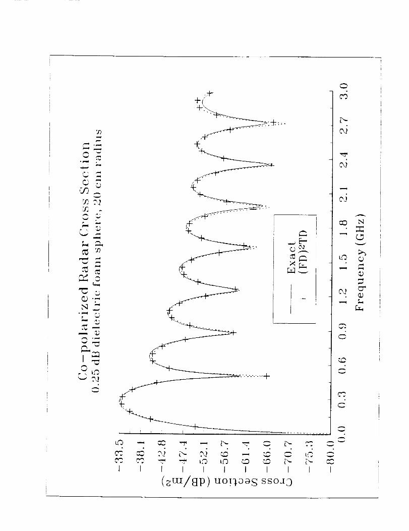
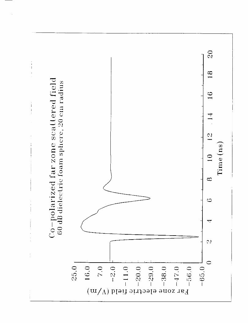
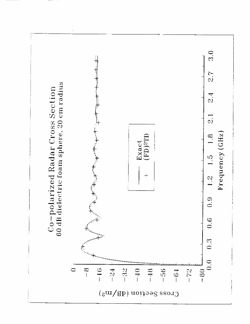
Figures 11-14 show the co-polarized far zone electric fieldversus time and the co-polarized RCS for the 0.25 dB and 60 dBdielectric foam spheres respectively.

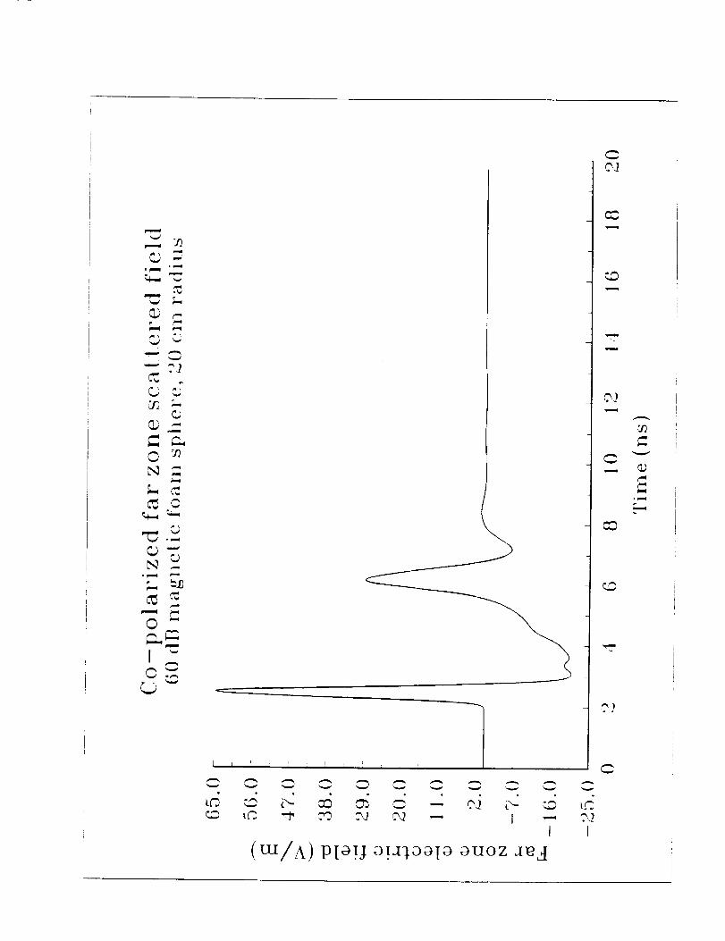
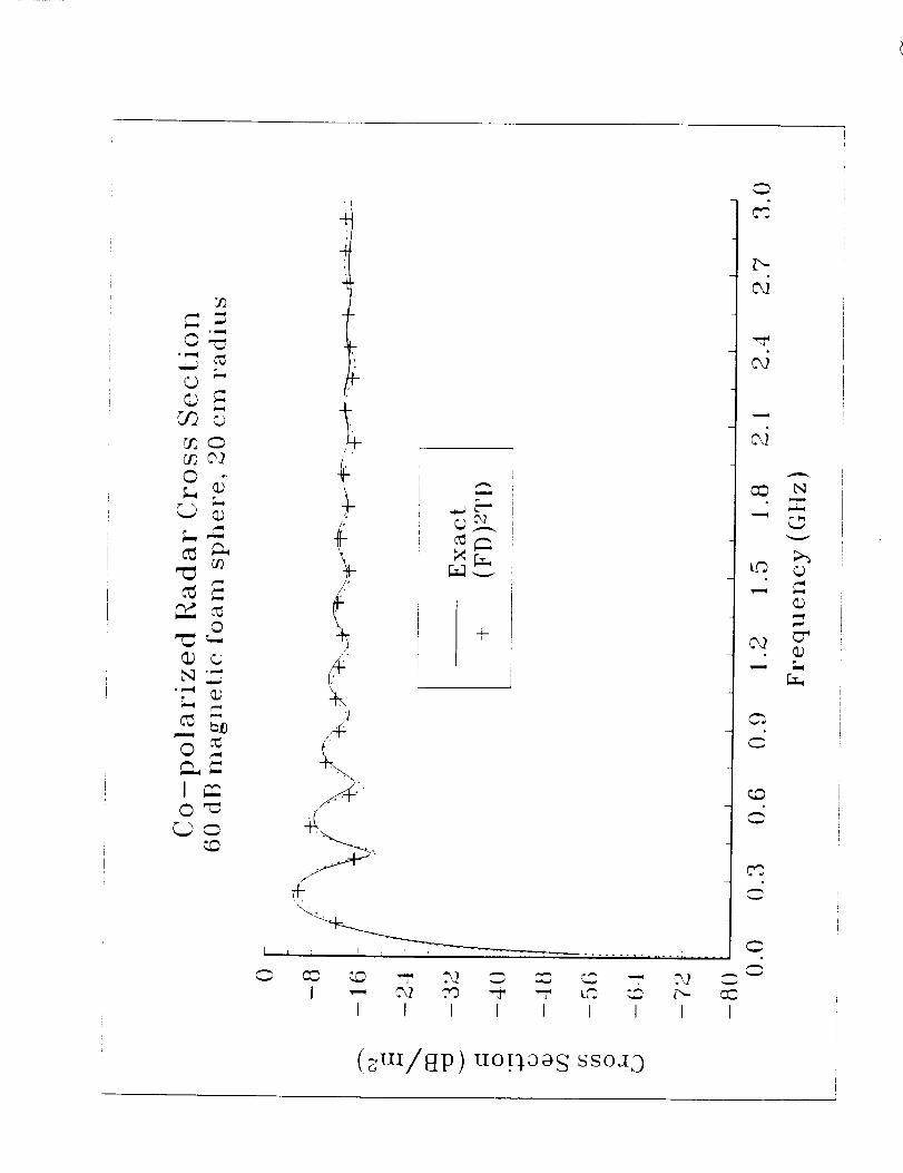
Figures 15-18 show the co-polarized far zone electric fieldversus time and the co-polarized RCS for the 0.25 dB and 60 dBmangetic foam spheres respectively.

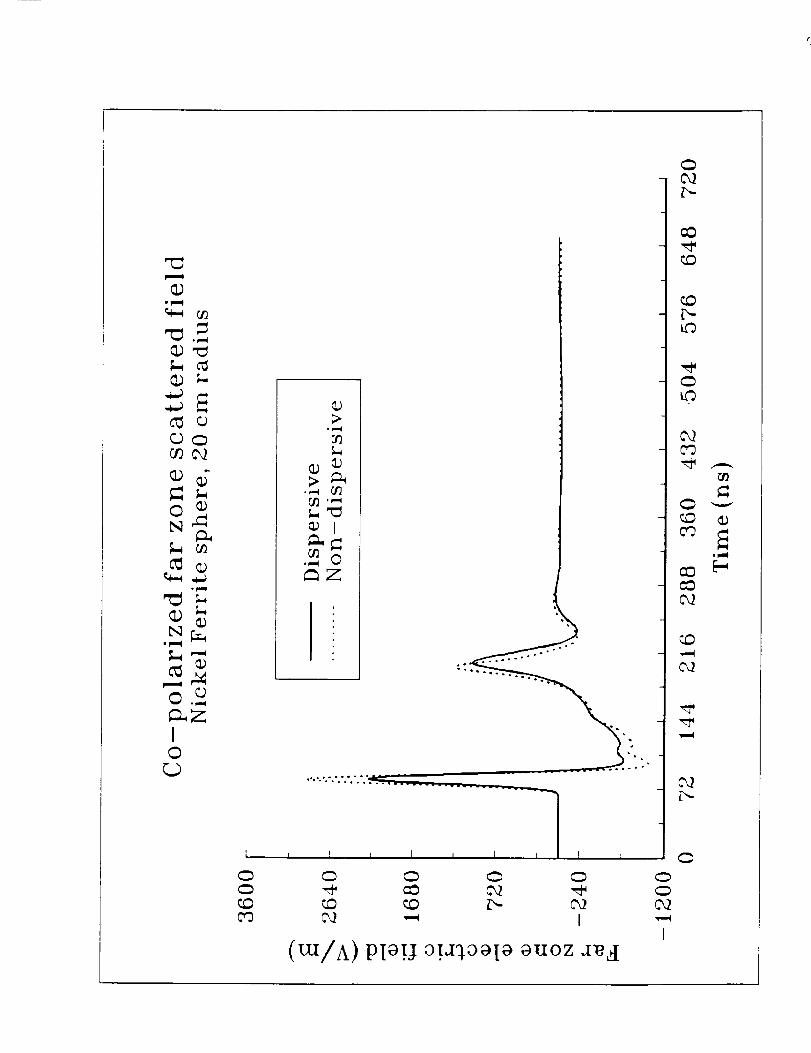
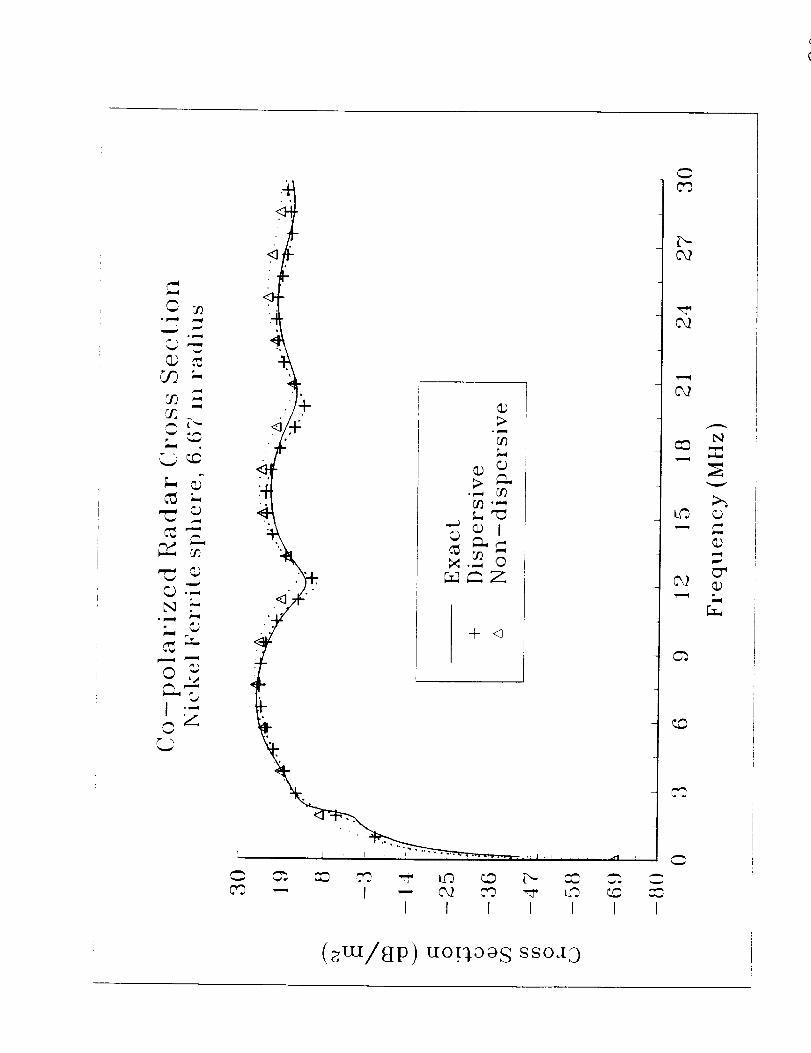
Figures 19-20 show the co-polarized far zone electric fieldversus time and the co-polarized RCS for the default NickelFerrite sphere using the dispersive FDTD method and the non-dispersive FDTD method. For the non-dispersive method, anequivalent permeability and magnetic conductivity were defined at30 MHz from (16) with _ replacing _ as

_r = _/ J ((_=2,30E6) ' CT" = OlJ,//_O J ((_=21r30E6)

XI. SAMPLE PROBLEM SETUP

The code as furnished models a 6.67 m radius Nickel Ferrite

dispersive magnetic sphere and computes backscatter far zone

scattered fields at angles of 8=22.5 and 4=22.5 degrees. The

corresponding output data files are also provided, along with a

code to compute Radar Cross Section using these data files. In

order to change the code to a new problem, many different

parameters need to be modified. A sample problem setup will now

be discussed.

Suppose that the problem to be studied is RCS backscatter

versus frequency from a 28 cm by 31 cm perfectly conducting plate

with a 3 cm dielectric coating with a dielectric constant of 4E 0

using a 8-polarized field. The backscatter angles are 8=30.0 and

4=60.0 degrees and the frequency range is up to 3 Ghz.

Since the frequency range is up to 3 Ghz, the cell size must

be chosen appropriately to resolve the field IN ANY MATERIAL at

the highest frequency of interest. A general rule is that the

cell size should be i/I0 of the wavelength at the highest

frequency of interest. For difficult geometries, 1/20 of a

wavelength may be necessary. The free space wavelength at 3 GHz

is 10=10 cm and the wavelength in the dielectric coating at 3 GHzis 5 cm. The cell size is chosen as 1 cm, which provides a

resolution of 5 cells/l in the dielectric coating and i0 cells/l 0

in free space. Numerical studies have shown that choosing the

cell size _ 1/4 of the shortest wavelength in any material is

the practical lower limit. Thus the cell size of 1 cm is barely

adequate. The cell size in the x, y and z directions is set in

the common file through variables DELX, DELY and DELZ. Next the

problem space size must be large enough to accomodate the

21

scattering object, plus at least a five cell boundary (i0 cells

is more appropriate) on every side of the object to allow for the

far zone field integration surface. It is advisable for plate

scattering to have the plate centered in the x and y directions

of the problem space in order to reduce the cross-polarized

backscatter and to position the plate low in the z direction to

allow strong specular reflections multiple encounters with the

ORBC. A i0 cell border is chosen, and the problem space size is

chosen as 49 by 52 by 49 cells in the x, y and z directions

respectively. As an initial estimate, allow 2048 time steps so

that energy trapped within the dielectric layer will radiate.

Thus parameters NX, NY and NZ in COMMOND.FOR would be changed to

reflect the new problem space size, and parameter NSTOP is

changed to 2048. If all transients have not been dissipated

after 2048 time steps, then NSTOP will have to be increased.

Truncating the time record before all transients have dissipated

will corrupt frequency domain results. Parameter NZFZ must be

equal to 1 since we are interested in far zone fields only.

Parameter MAGNET must be equal to 0 for the dielectric scatterer.

To build the object, the following lines are inserted into theBUILD subroutine:

C

C

C

C

C

C

BUILD THE DIELECTRIC SLAB FIRST

ISTART=II

JSTART=II

KSTART=II

NXWIDE=28

NYWIDE=31

NZWIDE=3

MTYPE=2

CALL DCUBE(ISTART,JSTART,KSTART,NXWIDE,NYWIDE,NZWIDE,MTYPE)

BUILD PEC PLATE NEXT

ISTART=II

JSTART=II

KSTART=II

NXWIDE=28

NYWIDE=31

NZWIDE=0

MTYPE=I

CALL DCUBE(ISTART,JSTART,KSTART,NXWIDE,NYWIDE,NZWIDE,MTYPE)

The PEC plate is built last on the bottom of the dielectric

slab to avoid any air gaps between the dielectric material and

the PEC plate. In the common file, the incidence angles THINC

and PHINC have to be changed to 30.0 and 60.0 respectively, the

cell sizes (DELX, DELY, DELZ) are set to 0.01, and the

polarization is set to ETHINC=I.0 and EPHINC=0.0 for 8-polarized

fields. Since dielectric material 2 is being used for the

dielectric coating, the constitutive parameters EPS(2) and

22

SIGMA(2) are set to 4£o and 0.0 respectively, in subroutineSETUP. This completes the code modifications for the sampleproblem.

XII. NEW PROBLEM CHECKLIST

This checklist provides a quick reference to determine if

all parameters have been defined properly for a given scattering

problem. A reminder when defining quantities within the code:

use MKS units and specify all angles in degrees.

COMMOND.FOR:

i) Is the problem space sized correctly? (NX, NY, NZ)

2) For near zone fields, is the number of sample points correct?

(NTEST)

3) Is parameter NZFZ defined correctly for desired field

outputs?

4) Is parameter MAGNET defined correctly for the type of

scatterer?

5) Is the number of dispersive dielectric (NEDISP) and

dispersive magnetic (NHDISP) materials defined correctly?

6) Is the number of time steps correct? (NSTOP)

7) Are the cell dimensions (DELX, DELY, DELZ) defined correctly?

8) Are the incidence angles (THINC, PHINC) defined correctly?

9) Is the polarization of the incident wave defined correctly

(ETHINC, EPHINC)?

i0) For other than backscatter far zone field computations, are

the scattering angles set correctly? (THETFZ, PHIFZ)

SUBROUTINE BUILD:

i) Is the object completely and correctly specified?

SUBROUTINE SETUP:

i) Are the constitutive parameters for each material specified

correctly? (EPS, XMU, SIGMA, SIGMAC)

2) Are the constitutive parameters for each dispersive material

defined correctly? (EPSSTA, EPSINF, RELAXT, RELSIG, XMUINF,

XMUSTA, RELAXT, RELSIG)

23

FUNCTIONS SOURCEand DSRCE:

i) If the smooth cosine pulse is not desired, is it commentedout and the Gaussian pulse uncommented?

SUBROUTINEDATSAV:

i) For near zone fields, are the sampled field types and spatiallocations correct for each sampling point? (NTYPE, IOBS, JOBS,KOBS)

XIII. REFERENCES

[1] K. S. Yee, "Numerical solution of initial boundary value

problems involving Maxwell's equations in isotropic media,"

IEEE Trans. Antennas Propaqat., vol. AP-14, pp. 302-307, May1966.

[2] G. Mur, "Absorbing boundary conditions for the Finite-

Difference approximation of the Time-Domain Electromagnetic-

Field Equations," IEEE Trans. Electromaqn. Compat., vol.

EMC-23, pp. 377-382, November 1981.

[3] R. J. Luebbers et. al., "A Finite Difference Time-Domain

Near Zone to Far Zone Transformation," IEEE Trans. Antennas

Propagat., vol. AP-39, no. 4, pp. 429-433, April 1991.

[4] C. Balanis, Advanced Enqineerinq Electromaqnetics, New York:

Wiley, 1990, pp. 83-84.

[5] R. J. Luebbers et. al., "A frequency-dependent Finite-

Difference Time-Domain formulation for dispersive

materials," IEEE Trans. Electromaqn. Compat., vol. EMC-32,

pp. 222-227, August 1990.

[6] R. J. Luebbers et. al., "A frequency-dependent Finite-

Difference Time-Domain formulation for transient propagation

in plasma," IEEE Trans. Antennas Propaqat., vol. AP-39, pp.

429-433, April 1991.

[7] R. Holland, L. Simpson, K. S. Kunz, "Finite-Difference

Analysis of EMP Coupling to Lossy Dielectric Structures,"

IEEE Trans. Electromaqn. Compat., vol. EMC-22, pp. 203-209,

August 1980.

XI. FIGURE TITLES

Fig. 1 Standard three dimensional Yee cell showing placement

of electric and magnetic fields.

Fig. 2 Real part of relative permeability versus frequency for

0.25 dB magnetic foam.

Fig. 3

Fig. 4

Fig. 5

Fig. 6

Fig. 7

Fig. 8

Fig. 9

Fig. i0

Fig. Ii

Fig. 12

Fig. 13

Fig. 14

Fig. 15

Fig. 16

Fig. 17

Fig. 18

24

Imaginary part of relative permeability versusfrequency for 0.25 dB magnetic foam.

Relative magnetic susceptibility versus time for 0.25dB magnetic foam.

Real part of relative permeability versus frequency for60 dB magnetic foam.

Imaginary part of relative permeability versusfrequency for 60 dB magnetic foam.

Relative magnetic susceptibility versus time for 60 dBmagnetic foam.

Real part of relative permeability versus frequency forNickel Ferrite with _s = i00, _® = I, r o = 20 ns.

Imaginary part of relative permeability versus

frequency for Nickel Ferrite with _s = i00, _® = i, _0

= 20 ns.

Relative magnetic susceptibility versus time for NickelFerrite.

Co-polarized far zone scattered field versus time for

0.25 dB dielectric foam sphere with 20 cm radius.

Co-polarized Radar Cross Section versus frequency for

0.25 dB dielectric foam sphere with 20 cm radius.

Co-polarized far zone scattered field versus time for

0.25 dB magnetic foam sphere with 20 cm radius.

Co-polarized Radar Cross Section versus frequency for

0.25 dB magnetic foam sphere with 20 cm radius.

Co-polarized far zone scattered field versus time for

60 dB dielectric foam sphere with 20 cm radius.

Co-polarized Radar Cross Section versus frequency for

60 dB dielectric foam sphere with 20 cm radius.

Co-polarized far zone scattered field versus time for

60 dB magnetic foam sphere with 20 cm radius.

Co-polarized Radar Cross Section versus frequency for

60 dB magnetic foam sphere with 20 cm radius.

25

Fig. 19 Co-polarized far zone scattered field versus time forNickel Ferrite sphere with 6.67 m radius using bothdispersive FDTD and non-dispersive FDTD.

Fig. 2O Co-polarized Radar Cross Section versus frequency for

Nickel Ferrite sphere with 6.67 m radius using both

dispersive FDTD and non-dispersive FDTD.

z

(i,j ,k+!)

x (i, j, k+l)/

(i+l,j,k+l)

Ez(i+l' J'k) i

(i+l, j ,k)

/J

,//

Ey(i,j,k+l)

"_ i

i

Hz(i,j ,k+l)

!

Ey(i+l,j ,k+l)

E z (i,j ,k) I

i]

I2=>

Hy(±, jl, k)

Hx(i÷l,j

! /_,/

( ±, j, k_: :_

//

_x (i,j ,k)

.©Hx(i,j ,k)

--'r--

,k)

Ey (i+l,j,k)

][ Ey (i,j,lk)

Hz(i, j ,k)

__£_

i,j+l,k+l)

• !

x(i,ji÷l,k+l)!I

(i+l,j+l,k+l)

i

i

///

/

(i÷l,j÷l,k)

Ez(i,j+l,k)

_Hy(: i,j+l,k)

Ez(i÷l,j÷l,k)P

(i,j+l,k)

_x(i,j+l,k)

Y

x

,_mq

wm-,_

°jM_

©

Jj'

!

!

//

/J

JJ

JJ

fif i I i _

C_

C_

C_

qFmu_

C_

C_

_q

,.,..,op,--_

,p.--_

,...,

,.---,

\\

\

,,._., ,--. ,_., _ .,

I I I I I I I I I

{ arf } tu I

t"--

ty_

C

I

N

©

o_,,4

f_

@

m

w

N

©

j

(60I X) u_

_D

o_

©

C

W

C

I

/iJ

/f

i i

,/"

t

J

J

ill i I

,f

_J

>_

°_,--_

° p..._

,.Q

© 0

© ,..,

©

_C

°_

_aD

L

G

I I I I I I I I

{_r/} ua I

C'?

0_

0_

I

N

q)

©

.P..I

© ,-.> ,-,

°_

W

0o_..q

I i [ i i I ....

/

,51

©

(60I Xt t_

w_

.llm_

JJ_

D _

.i,m_

©

©,-.

*l=Jl

Z

//

!

//

/

//

1//

/

//

///

/

ii /

Ji/

C_

=_

L_

,o _

C_

©

© II

W

©II

W

P

"Z

\\

\

\

\

\

k,

\

\\

J

JJ

JI J ' , ' i ,

I I I I I I I I

'\

//

,o

u_

I

{_H} ml

©

©

._,,_

¢,,/

[-.

¢:0

C

(60I X) _u_

_,) ","

G_ '-'

c,.) _.,

© ,-.S

_u...

e_ "-'..., "U

I ko

I

I I I I I

(tu/A) pIo.tj a!al, ao[o ouoz ze A

G/

,-'m

I

©

© .,:uo_ml •

o

+(

_-o -. OoOoOo-..°o._

_.T....]_

___ .......... t °,

I I I I I I I I I

(ztu/_iP) uo.[_ooS sso_o

L.4t"--

I

CO

I",-

O2

¢q

h_

0

¢.O

C

¢,9

C

I

©

¢)

k,

_d© a.,

e_

0 ,"S

0

° P'q

N --,

0_

o_.

I I I I

(m/A) pIo.U o!aloo[o ouoz aej

I

00,t

t.D

C

0_

¢)

b-,

r_

° _-,,I

¢) =

C/3C

OQ¢_/

©

e-,

tq ¢_

_-)ea

+

1 i , ; _ ' : 1 I 1 __ ....... 1o- -_-,

I I I I I I I I I I

(_Ua/Hp) uo_aaS ssoao

=

C

I

oJ,1

p

_d

N

N• ,"'q _

©o

i

_d d¢X/ ,"-,

! |1 ; _ [ i ' '

I I I 1

(u-Z/A) PIO!J o!.zlooIo ouoz ae_I

¢.D

",- t£'? :.D

I I I

c

©

.p,,_

I

,q

F

/,

!+

I I I I I

C

C_

u_

m

c_

G

cc.

...... i.....

I I I I

_q

(z_u/HP) uo._]ooS sso_ O

© -• j,,,q

D -J_

©¢) ,.-

N ""

¢)--

0 *"

I "0

L

_4¢D

L i r I I

cz _ ,,,-4; - ._ c--

I

(m/A) p[a.U o!.t:loaia auoz aez[

¢,,/

,.-, ©

a.

C

i

,p,,_

0

oe

0

w

A

V

/_°"

÷

¢.

I I I I I I I I I

b_

©

(ztu/_p) uo!loaS sso_3

op,,_

OG

Na:

°_,,_

_DN_

I0

L

0

¢0

>°pm_

>

_Z

(m/A) pIa!J o!a_aaIa ouoz a_d

t',-

t"-

tr'a

¢o

W°_

,_ i. _.-

,_ oo

I ""0 Z

1

I I I I I I I

[-,..

c_

_D

N

0

(_m/Sp) uo.[looS ssoao