USER MANUAL - cdn.cloud1.cemah.net · • Microsoft Windows 9x/NT/2000 Operating System; ... Baird & Associates 1-4 User Manual - Nemadji River Sediment Transport Modeling 1.4 Hardware

PREPARED FOR:

U.S. ARMY CORPS OF ENGINEERS, DETROIT DISTRICT

PREPARED BY:

W.F. BAIRD & ASSOCIATES COASTAL ENGINEERS LTD.

AUGUST 2000

UUSSEERR MMAANNUUAALLNemadji River

Sediment Transport Modeling

This report has been prepared for U.S. Corps of Engineers by:

W.F. BAIRD & ASSOCIATES COASTAL ENGINEERS LTD.627 Lyons Lane, Suite 200, Oakville, Ontario, L6J 5Z7

For further information please contact:

Steve Langendyk: 905-845-5385 ext. 23, orQimiao Lu: 905-845-5385 ext. 24.

Baird & Associates User Manual - Nemadji RiverSediment Transport Modeling

TABLE OF CONTENTS

1. INTRODUCTION.............................................................................................1-1

1.1 About This Manual .................................................................................................................................1-1

1.2 Manual Format.......................................................................................................................................1-2

1.3 File Types.................................................................................................................................................1-3

1.4 Hardware and Software Requirement ................................................................................................1-4

1.5 Installation ...............................................................................................................................................1-4

1.6 Contact Information...............................................................................................................................1-4

2. WATERSHED DELINEATION USING GIS ................................................2-1

2.1 Introduction .............................................................................................................................................2-1

2.1.1 The ArcView Environment and Extensions..................................................................................2-1

2.2 Digital Elevation Model Datasets.........................................................................................................2-2

2.2.1 Sourcing and Acquiring USGS DEM Datasets ...........................................................................2-2

2.2.2 Importing and Using USGS DEM Datasets into ArcView GIS.................................................2-2

2.3 Flow Direction.........................................................................................................................................2-4

2.4 Flow Accumulation ................................................................................................................................2-5

2.5 Watershed Extraction ............................................................................................................................2-6

2.6 Generating Subwatershed ‘Catchment Areas’ ..................................................................................2-8

3. SUBWATERSHED-BASED CURVE NUMBER VALUATION USING GIS...........3-1

3.1 Introduction .............................................................................................................................................3-1

3.2 SCS Method.............................................................................................................................................3-1

3.3 Integrating Multiple Source Datasets For Cn Valuation..................................................................3-3

3.3.1 Combining Catchment Area and Soils ..........................................................................................3-4

3.3.2 Extracting Land Use Data for the Watershed..............................................................................3-7

3.3.3 Intersect Catchment Area-Soils Dataset with Land Use Dataset ...............................................3-7

3.4 Calculating Area-Weighted Curve Number Values ..........................................................................3-8

3.4.1 Calculate Area for Each Catchment Polygon...............................................................................3-8

3.4.2 Create a Key Field ............................................................................................................................3-9

3.4.3 Curve Number Lookup Table .......................................................................................................3-10

3.4.4 Link Curve Number Values To Unique Polygon Areas ............................................................3-11

3.4.5 Calculate the Proportional Curve Number Value for Each Catchment Area ........................3-11


4. RAINFALL-RUNOFF AND HYDRODYNAMIC MODEL......................................4-1

4.1 Introduction .............................................................................................................................................4-1

4.2 Change CN values for land use change...............................................................................................4-1

4.2.1 Input ..................................................................................................................................................4-1

4.2.2 Output................................................................................................................................................4-1

4.2.3 Operations.........................................................................................................................................4-2

Step 4.2.1 Reorder CN table and Calculate Lag-Time ..........................................................................4-2

Step 4.2.2 Open MIKE11 Simulation Project .......................................................................................4-4

Step 4.2.3 Edit RR model parameters ....................................................................................................4-4

4.3 Prepare Boundary Conditions for a Storm Event .............................................................................4-5

4.3.1 Input ..................................................................................................................................................4-5

4.3.2 Output................................................................................................................................................4-5

4.3.3 OperationsStep 4.3.1 Prepare hourly precipitation data.............................................................4-5

Step 4.3.1 Prepare hourly precipitation data .........................................................................................4-6

Step 4.3.2 Estimate water level at downstream boundary.....................................................................4-7

Step 4.3.3 Open a simulation project .....................................................................................................4-8

Step 4.3.4 Edit Boundary Condition Data .............................................................................................4-8

Step 4.3.5 Edit RR Parameter Data........................................................................................................4-9

4.4 Run the Model.......................................................................................................................................4-10

4.4 Run the Model.......................................................................................................................................4-10

4.4.1 Input ................................................................................................................................................4-10

4.4.2 Output..............................................................................................................................................4-10

4.4.3 Operation.........................................................................................................................................4-10

Step 4.4.1 Open a simulation project ...................................................................................................4-10

Step 4.4.2 Set inputs and Run model....................................................................................................4-10

4.5 View and Export model results to Sediment Transport model.......................................................4-11

5. SEDIMENT LOADING MODEL .......................................................................5-1

5.1 LOADING THE EXTENSION.............................................................................................................5-1

5.2 INPUTS....................................................................................................................................................5-1

5.3 USING THE EXTENSION ...................................................................................................................5-2


6. ASSESSING LAND USE CHANGE ..................................................................6-1

6.1 Introduction .............................................................................................................................................6-1

6.2 Input..........................................................................................................................................................6-1

6.3 OUTPUT..................................................................................................................................................6-1

6.4 OPERATIONS........................................................................................................................................6-1

Baird & Associates 1-1 User Manual - Nemadji RiverSediment Transport Modeling

USER MANUALUSER MANUALSEDIMENT TRANSPORT MSEDIMENT TRANSPORT MODELING SYSTEM IN ODELING SYSTEM IN

NEMADJI RIVER BASINNEMADJI RIVER BASIN

1. INTRODUCTION

1.1 About This Manual

A modeling system has been developed to assess sediment loading in the Nemadji River Basin. This manual is prepared for users who use this modeling system to assess the impact of land use change on sediment load in the Nemadji River Basin and its tributaries.The Nemadji Sediment Transport Modeling (NSTM) system consists of four components:

Spatial Database Preparation - GIS Component;

Rainfall-Runoff (Hydrological) modeling;

Hydrodynamic Modeling;

Sediment Transport Calculations.

The conceptual links of these four system components are shown in Figure 1. The GIS component provides preparations of all spatial databases which are used are as inputs tothe hydrological modeling and hydrodynamic modeling. The hydrological model calculates runoffs for all catchments for inputs to the hydrodynamic model. The hydrodynamic model simulates the hydrodynamics in the rivers and provides hydrodynamic parameters such as velocity, water depth and discharge to the sediment transport component that calculates river erosion and sediment load. The details of these links are described in a companion technical report (Baird, 2000). The NSTM system has been calibrated for the Skunk Creek subwatershed and the Deer Creek subwatershed. These two subwatersheds are used to present the general concepts of the NSTM in specific examples.

This manual has been prepared for the U.S. Army Corps of Engineers, Detroit District by Baird & Associated, with contributions from the Detroit based firm Wade-Trim.


This manual is designed for users to operate this calibrated system for a range of land use conditions (including changing forestry practices) in the Skunk Creek and Deer Creek subwatersheds. The manual is suitable for users who are familiar with:

• Microsoft Windows 9x/NT/2000 Operating System;

• E.S.R.I. ArcView GIS Version 3.1 or higher;

• E.S.R.I. Spatial Analyst Version 1.1;

• D.H.I. MIKE 11;

• Microsoft-Excel.

1.2 Manual Format

This manual is divided into the following parts for each of the four model components describing:

• Description of Functions

• Input

• Output

• Operations

Topography,Landuse, Soils

GraphicPresentation

Curve numbers,slopes, areas

GIS (ArcView) Sediment loading,downcutting

Hydrological Modeling(Mike11, UHM)

Sediment Model(Excel Calculations)

Peak flows and runoff volumes Hydrodynamic Model

(Mike11-HD)Water levels

and velocities


1.3 File Types

Various types of the data are used in the system. The data type is identified by the file extension name. The data types used in the system are:

GIS Data:

*.shp, *.shx and *.dbf These 3 files together comprise an ArcView shapefile which is used to store GIS vector (point, line, area) features

MIKE11:

*.sim11 ...... Mike11 model simulation data

*.nwk11..... Mike11 River network data

*.bnd11...... Mike11 Boundary condition data

*.rr11 ......... Mike11 Rainfall-runoff model parameters

*.hd11........ Mike11 Hydrodynamic model parameters

*.xns11 ...... Mike11 Cross-section data

*.res11 ....... Mike11 model results

*.dfs0......... Mike11 Time series data

*.cla ........... Mike11 complete layout view data

To assist the user, a file format convention has been developed. Each data filename in this system consists of three name segments separated by dashes as follows: creek name or station name - storm event date (short date format: yymm) - variable name and the extension. For example, the file name: Holyoke-7808-Rainfall.dfs0 is the rainfall time series data file at the Holyoke meteorological station for the storm event of August 1978. A missing segment of the file name refers to data that can be applied in the whole range described in that segment data. For instance, the file name “Deer.nwk11” refers to the river network data for the Deer Creek, which can be applied for all storm events and all other simulations.


1.4 Hardware and Software Requirement

The NSTM system can only run on IBM-compatible personal computers with the Microsoft Windows Operating System. The minimum hardware and software requirements for the NSTM system are listed below:

Hardware:

• Pentium II or greater CPU

• 1 Gigabyte of free hard drive space

• 32MB of memory RAM

Software:

• Microsoft Windows 95;

• E.S.R.I. ArcView GIS Version 3.1;

• E.S.R.I Spatial Analyst Version 1.1;

• Danish Hydraulic Institute MIKE 11 Version 4.10 (one site license has been obtained for use with the Nemadji River Sediment Transport Modeling Project);

• Excel for Microsoft Office 95.

1.5 Installation

The NSTM system incorporates ArcView GIS, MIKE 11 and Excel software into an interactive system. These software packages should be installed prior to installing the NSTM. Please refer to the manuals of these packages for complete installation instructions.

Once the packages have been installed, the NSTM data sets can be loaded onto the computer. The NSTM system makes use of many data sets. These files have all beenpackaged onto a CD with a convenient installation package. To install the data sets on a computer, run “Setup.exe” from the CD from Explorer and follow the instructions on your screen.

1.6 Contact Information

Dr. Qimiao Lu or Steve LangendykW.F. Baird & Associates

Tel: (905) 845-5385, Fax: (905) 845-0698Email: [email protected], [email protected]

User Manual – Nemadji RiverSediment Transport Modeling

Baird & Associates 2-1

2. WATERSHED DELINEATION USING GIS

The overall watershed delineation process is described here, using the Nemadji River tributary Deer Creek as an example within ArcView GIS. Using this combination of data and software, however, the watershed delineation process described here can be applied to other Nemadji River watersheds assuming adequate digital base data is available.

This chapter assumes a minimal working knowledge of ArcView GIS. This chapter can be skipped for work with the Deer and Skunk Creek sub-watersheds, as data for these areas have already been prepared.

2.1 Introduction

A watershed boundary defines the drainage or catchment areas that contribute to a specified outlet channel such as a creek or river. A specific catchment area includes all the land that contributes (drains) to a central point. The overland drainage pattern is based on the topography of an area.

This drainage behaviour can be modeled within a GIS environment using a combination of datasets and analysis tools. The process described here will use Digital Elevation Model (DEM) datasets from the United States Geological Survey (USGS). DEMs consist of a sampled array of elevations for a number of ground positions at regularly spaced intervals called grids. The software used is ArcView GIS 3.x, from Environmental Systems Research Institute (ESRI), Redlands, California.

2.1.1 The ArcView Environment and Extensions

Additionally, two ArcView extensions developed by ESRI are used: Spatial Analyst v.1.1 which must be purchased separately; and Hydrologic Modeling v1.1, which is included with ArcView v3.1 and up but can only be installed if the Extension file (HYDROV11.AVX) is copied from its default location of ARCVIEW\SAMPLES\EXT\to ARCVIEW\EXT32\ and then the user adds the extension to the current ArcView project using File > Extensions.

The Hydrologic Analysis extension adds a new pull-down menu item “HYDRO” to the ArcView user interface. While the Hydrologic Analysis extension contains a tool that will automate the full process of delineating a complete watershed from a raw DEM, it is recommended that the user go through each step manually to inspect each new processed dataset for errors.



2.2 Digital Elevation Model Datasets

2.2.1 Sourcing and Acquiring USGS DEM Datasets

The USGS DEM dataset covers the entire United States. More information regarding USGS Digital Elevation Model Data can be found at:

http://edc.usgs.gov/glis/hyper/guide/usgs_dem

Appropriate datasets to support the analysis discussed here can be downloaded at the USGS Geographic Data Download page at:

http://edc.usgs.gov/doc/edchome/ndcdb/ndcdb.html

Several scales of DEM data are available, including 1:24,000 and 1:250,000. For this exercise, the larger-scaled 1:24,000 will be used. Compared to the 1:250,000 scale dataset, the 1:24,000 dataset provides a more detailed representation of the topography, but also results in a larger dataset. To cover the entire U.S. using 1:24,000 scale, the mapping is broken up into individual tile sheets that correspond to the USGS 1:24,000 scale topographic quadrangle map series for all of the United States and its territories.

Each DEM is based on a 30- by 30-meter cell data spacing, called a raster data model. In the raster model, geographic space is partitioned into equal sized square cells that collectively cover the entire geographic region under study. A raster grid exists in a Cartesian coordinate system, the rows and columns in the grid are parallel to the axes of the coordinate system, and each grid cell stores a numeric data value. This model is ideally suited to representing features that vary continuously over space such as temperature or elevation surface.

2.2.2 Importing and Using USGS DEM Datasets into ArcView GIS

The individual USGS DEM sheets are in a format called Spatial Data Transfer Standard (SDTS) that must be converted into ArcView GRID format. ArcView 3.2 contains a utility “SDTS Raster to Grid”. This utility must be run once for each individual DEM dataset.

If the watershed of interest extends beyond the boundary of one DEM sheet, adjacent sheets will each have to be converted into GRIDs and then merged together to form one GRID using the GRID > Merge request. The tile sheets as prepared by the USGS are all edge-matched so that they should line up perfectly with each other. Figure 2.1 shows 3



adjacent sheets for the Deer Creek area: Atkinson (red), Wrenshall (orange) and Frogner (green).

Figure 2.1 Individual Adjacent USGS DEM Tile Sheets (Deer Creek area)

Figure 2.2 shows a three-dimensional overview look at a DEM representation of a topographic surface, showing how the grids cells cover the entire surface.

Figure 2.2 Perspective View of DEM Surface (Deer Creek area)



A closer inspection with an exaggerated terrain relief reveals the ‘stepped’ nature of the dataset. An examination of Figure 2.3 reveals the 30- by 30-metercells as individual steps.

Figure 2.3 Exaggerated Terrain Relief (upper Deer Creek)

2.3 Flow Direction

For each cell within a DEM grid, the flow direction of water draining will be to one of its 8 neighbours, that cell with the steepest drop. By applying this procedure for each and every cell in the elevation GRID, the flow direction establishes an overall drainage pattern as water flows from one cell to another, and to another, and so on, until finally reaching the edge of the dataset.

A cell or group of cells that does not drain out to the edge would be considered a sink.This can occur when all 8 neighbouring cells are at a higher elevation. This essentiallycreates a sink, which is considered to have indeterminate flow direction. Sinks in elevation data are sometimes due to errors in the data due to sampling techniques and the rounding of elevation values to integer numbers.

To create a Flow Direction GRID that isolates these potential sinks, use the Hydrologic Modeling Extension function Hydro > Identify Sinks.

To create an accurate representation of flow direction it is best to use a dataset that is free of sinks. At this point, the flow direction grid only identifies sinks. A digital elevation model that has been processed to remove all sinks is referred to as a depressionless DEM,



which simplifies the DEM representation for drainage analysis. To create a depressionless DEM, simply use the Hydrologic Modeling Extension function Hydro > Fill Sinks on the DEM. Alternately, ArcView provides a sample script (“Spatial.DEMfill”) which illustrates the individual iterative steps to create a depressionless DEM. This script can be found in the online ArcView Help file. Simply cut and paste this script into a new ArcView Script document, compile and run it. Refer to the ArcView documentation ‘Using Avenue’ for more information on working with Scripts.

2.4 Flow Accumulation

Once the flow direction for each cell has been established, a flow accumulation grid can be generated from the flow direction dataset using the Hydrologic Modeling Extension function Hydro > Flow Accumulation. A flow accumulation grid represents the accumulated flow to each cell, by accumulating the weight for all cells that flow into each downslope cell.

Figure 2.4 Flow Accumulation

Figure 2.4 illustrates a grid of flow accumulation values, with light colours representing low accumulations, and darker colours representing higher accumulations. This provides a visual confirmation of the drainage patterns produced by the DEM created through the data processing steps outlined above.



2.5 Watershed Extraction

2.5.1 DEM Based Watershed Extraction

Using the flow direction grid dataset, it is possible to identify the contributing area above a location in the grid. In other words, identifying a watershed by selecting a drainage pour point, or watershed outlet. The datasets used thus far have included areas well beyond the extent of Deer Creek to ensure that all drainage areas would be captured. Using the flow direction and flow accumulation grids, it is possible to identify a watershed based on a user-specified point.

The adjacent ArcView Avenue code from the online Help creates a watershed based on a point that is specified with a cursor in the view. The watershed is presented as a new Grid in the View. It assumes that there is a single elevation Grid (Gtheme) active, and that the View contains a flow direction Grid named "Flow Direction" and a flow accumulation Grid named "Flow Accumulation". The example must be executed from an Apply event since it uses ReturnUserPoint to get the point.Associate the script with a button on the View buttonbar. Refer to the ArcView document ‘Using Avenue’ for more information regarding the use of scripts.

theView = av.GetActiveDoctheDisplay = theView.GetDisplaytheGridTheme = theView.GetActiveThemes.Get(0)theGrid = theGridTheme.GetGridthePoint = theDisplay.ReturnUserPointmPoint = MultiPoint.Make({thePoint})theSrcGrid = theGrid.ExtractByPoints(mPoint,Prj.MakeNull,FALSE)theFlowDir = theView.FindTheme("Flow Direction").GetGridtheAccum = theView.FindTheme("Flow Accumulation").GetGridtheWater = theFlowDir.Watershed(theSrcGrid.SnapPourPoint(theAccum,240))' create a theme

theGTheme = GTheme.Make(theWater)' check if output is okif (theWater.HasError) then return NIL end' add theme to the view



Using this Avenue code, it is possible to extract out just the Deer Creek tributary watershed into a new grid. This drainage/catchment area represents the spatial extents that are of interest from here on.

Figure 2.5 Deer Creek Watershed

This watershed grid should be converted to a binary mask grid, with all of the grid cells containing just one value “1”, and the remainder of the grid being “No Data”. Do this using the Analysis > Map Calculator or Analysis > Reclassify. The new binary mask grid representing the Deer Creek subwatershed is used to “clip out” or extract a new DEM from the larger DEM using the Map Calculator.

Figure 2.6 highlights the extracted Deer Creek watershed by coloringits DEM against a greyscale hillshaded backdrop.




2.6 Generating Subwatershed ‘Catchment Areas’

From the Deer Creek watershed DEM, new Flow Direction and Flow Accumulation grids can be generated. These grids are required to delineate smaller catchments areas within the larger Deer Creek watershed. The Hydrologic Modeling extension allows the use of threshold values to delineate subcatchment areas within a watershed. The overall Deer Creek watershed is approximately 5000 acres. Deer Creek was divided into approximately 25 equally sized catchment areas. Choosing the number of catchment areas provides a balance between data analysis and data detail. The number of catchment areas will vary for each watershed, depending upon its size and other variables.


To delineate the catchment areas, use the Hydrologic Modeling Extension’s Watershedfunction, which will require the Flow Direction and Flow Accumulation grids. The Watershed function will also require a value denoting the minimum number of cells to form a watershed. The larger this threshold value, the larger the size of the catchments areas and the smaller the quantity of catchment areas.

The following page shows the results of three different threshold values applied to the same watershed area.

At this point, the defined watersheds are ready for incorporation into the hydrologic analysis.



Cell Count Threshold: 1000

Number of Catchments 7


Number of Catchments: 19


Number of Catchments: 31



3. SUBWATERSHED-BASED CURVE NUMBER VALUATION USING GIS

3.1 Introduction

The NSTM system is setup to use the Soil Conservation Service (SCS) method for determining peak flows and runoff volumes from sub-watersheds. For this reason, a GIS-based methodology was setup to generate the required input variables to this method.ArcView GIS will be used to determine catchment area, Curve Numbers, and watershed slope.

3.2 SCS Method

The Soil Conservation Service Runoff Curve Number or CN value is used to convert storm rainfall to runoff. Curve numbers provide a way of describing how quickly and to what extent storm rainfall becomes runoff for a particular area. Major contributing factors include land use cover and soil type. The relationship to determine runoff is:

Q = (I - 0.2 S)^2 / (I + 0.8S)(U.S. Department of Agriculture, Soil Conservation Service, SCS National Engineering Handbook, 1972)

where,

Q = direct surface runoff depth (mm )

I = storm rainfall (mm)

S = maximum potential difference between rainfall and runoff, starting at the time the storm begins (mm)

S = 25,400/CN – 254(U.S. Department of Agriculture, Soil Conservation Service, SCS National Engineering Handbook, 1972)

where, CN = the runoff curve number (dimensionless)

Curve numbers have been developed by the Soil Conservation Service to describe the characteristic land use, treatment or practice, hydrologic condition, hydrologic soil group, and antecedent moisture condition of a sub-watershed. Land use defines whether the area is agricultural, suburban or urban land. Treatment refers to agricultural practices such as straight row, terraced or contoured farming. The hydrologic condition (poor, fair, good) refers to a number of factors that tend to increase or decrease runoff (i.e. density of vegetative canopy or degree of surface roughness). The hydrologic soil group refers to the general nature of the underlying soil and is classified as:



A Soils with high infiltration rates (8 to 11 mm per hour) B Soils having moderate infiltration rates (4 to 8 mm per hour) C Soils having slow infiltration rates (1 to 4 mm per hour) D Soils having very slow infiltration rates (0 to 1 mm per hour)(from U.S. Department of Agriculture, Soil Conservation Service, SCS National Engineering Handbook, 1972)

For more information, refer to U.S. Department of Agriculture, Soil Conservation Service, SCS National Engineering Handbook, 1972 and the Minnesota Handbook of Hydrology.

Curve numbers for various conditions were developed by the SCS from studies of gaged watersheds. The CN value takes into consideration the initial abstraction which consists of interception, infiltration, and depression storage.

Table 3.1: Nemadji River CN Values

Hydrologic Soil GroupLanduse B

(MN253-254-257)C

(MN258)D

(MN475)Open 74 82 86Wetland 95 95 95Coniferous forest 70 76 77Deciduous forest 76 81 83Mixedwood forest 75 80Cultivated land 72 86 91Farmsteads and rural residences 83 93Grassland 59 70 77Open water & wetlands 95 95 95Open land 75 78 84Harvested 81 81 89

The CN matrix of values presented here are specific to Deer Creek and have been developed following a calibration procedure and should not be changed without recalibration. This table is the base information used to create lookup table in Section 3.4.3.

The land use and soil type dataset themes are readily available in GIS data formats. Each theme separately describes features as shapes with attributes. This information needs to be combined with catchment delineations developed earlier. Integrating these separate layers of information while preserving only the features within the spatial extent common to both themes (the watershed) is accomplished using the standard GIS spatial operator Intersect.



3.3 Integrating Multiple Source Datasets For Cn Valuation

To generate CN values for each catchment area, three datasets are combined, but only two can be intersected at a time. The order makes no difference for the final output, but by first combining the watershed catchment areas with the soils delineations it is possible to create an intermediate dataset that can be combined with a more dynamic land use dataset. This affords more flexibility in modifying the land use dataset, and combining it with the established Catchment-Soils dataset.

The individual datasets are representations of a particular theme. Each dataset theme delineates boundaries around common elements forming polygons. As datasets arecombined and intersected, the number of polygons increases as their geometry is integrated. Figure 3.1 illustrates how combining multiple data sets creates small polygons.Each polygon within a dataset also has various attributes associated with it. As the polygons are combined, their attributes are aggregated as well.

Figure 3.1 Intersecting Multiple Datasets



3.3.1 Combining Catchment Area and Soils

Within a catchment area, multiple soil types may be present. Along these boundaries thecatchment polygons will be split into new separate polygons. This is a common GIS spatial operation called Intersect. The new resultant polygon holds the attributes common to the two intersecting polygons.

Figure 3.2 Soil Boundaries on Catchment Areas



The GIS spatial operator Intersect is part of a group of tools loaded with the Geoprocessing Extension, an optional ArcView extension, and is accessed from the pull-down menu View > GeoprocessingWizard.

Select Intersect two Themes operation.

Figure 3.3 Geoprocessing Wizard

Select the watershed and soil themes as the input and overlay themes, andidentify an output theme to store the results.

Figure 3.4 Geoprocessing Wizard

As these datasets are combined, they combine not only geometric shape information, but also carry across important attribute information. Each polygon now contains both complete attribute tables from both source watershed and soil themes. This theme will be referred to as ‘Intersect A’.

Figure 3.5 Intersection of Soils and Catchment Areas



Below is a simplified view of the attribute tables, where each row represents a unique area (polygon), and each column is an attribute field. The resulting Intersected attribute table combines attribute information from each of the source contributing themes.

Catchment Area Attribute Table Soils Attribute Table

PolygonID CatchmentID

Area(sq.m)

1 A 45312 B 84633 C 54934 D 51965 E 48616 F 46837 G 60158 H 3987

Resulting Intersected Attribute Table

Soil classArea

(sq.m)MN253 19605MN258 17135MN254 12054MN257 20384MN475 48720

polygonID Catchment ID Soil Class1 A MN2542 B MN4753 C MN2543 C MN2574 D MN2545 E MN2535 E MN2548 H MN2538 H MN254



3.3.2 Extracting Land Use Data for the Watershed

The next step involves extracting the land use delineations for the watershed area of interest.

Use the Geoprocessing Wizard’s Clip One Theme Based on Anotherfunctionality to clip the land use using the watershed boundary andextract only the watershed’s land use.

Figure 3.6 Clipped Land Use to the Watershed Boundary

3.3.3 Intersect Catchment Area-Soils Dataset with Land Use Dataset

Using the Intersect Two Themes operation again, intersect the clipped land use delineations with the Intersect A theme (from 3.3.1), to produce a new theme, Intersect B.This theme will have many more polygons, each polygon carrying all of the attributes of the three source themes: catchment area, soil type and land use classification. In theDeer Creek example, there are now over 500 discrete continuous areas.

Figure 3.7 Intersect of Soils, Catchment Areas and Land Use



3.4 Calculating Area-Weighted Curve Number Values

The Intersect B theme has attribute information from all three source themes that were intersected to create it: catchment areas, soils, and land use. Using a combination of operators, area-weighted Curve Number values for each catchment area will now be calculated.

3.4.1 Calculate Area for Each Catchment Polygon

Begin by calculating the area for each polygon. This can be accomplished using the ArcView sample script ‘calcapl.ave’ which calculates feature geometry (area and perimeter) for individual polygon objects within a theme. Verify the creation of two new fields (Area and Perimeter) in the attribute table, and ensure that the units are meters.

As an extension to the area calculation, it is necessary to calculate the proportional area for each polygon within each catchment watershed. This is required to calculate the areaweighted CN value of each polygon in relation to the watershed catchment area that it is a part of. Follow the 8 steps below to calculate the proportional area for each polygon in the Intersect B theme.

1. Open the theme attribute table and select the WATERSHED field by clicking on the column header.

2. Choose Summarize from the Field pull down menu.

3. In the Summary Table Definition window, identify the output file as ‘Watershed_Total_Area.dbf’. From the Field drop down list choose ‘AREA’. From the Summarize By drop down list choose ‘SUM’. Click on the Add button and ‘SUM_AREA’ will be added to the list in the bottom right of the window. Click OK.



4. A quick inspection of the Watershed_Total_Area.dbf file reveals that it shares a common field with the Intersect B attribute table: WATERSHED. This is called the key field and will be used to join the summary table to the Intersect B table. In the Watershed_Total_Area.dbf table, click on the WATERSHED heading button. Switch to the Intersect B table and click on the WATERSHED heading button. Append the fields from the summary table to the Intersect B table using the Join command under the Table pull down menu. The fields from the summary table are now part of the attribute table.

5.Create a new field to store the proportional area called PROP_AREA with the following parameters: Type: Number; Width 10; Decimal Places: 6.

6 Using the calculator command, calculate proportional area as being equal to Areadivided by Total Area. Save and stop editing the table.

3.4.2 Create a Key Field

Continue by opening the attribute table of Intersect B and adding a new field called ‘CN_Key’ (string, 50 characters).Highlight this new field and using the Field > Calculate command, create the expression CN_Key = Soils ++ Landuse. The use of two plus signs is interpreted by ArcView as concatenate with a space.

In the example case of Deer Creek, a CN_Key value is generated for each of the over 500 polygons. But there is significantly less unique combinations of soil and land use. A list of unique values can be generated and stored in a separate table called a Lookup Table.



3.4.3 Curve Number Lookup Table

Continue by creating a lookup table of Curve Number values that match the soils/land use matrix presented at the beginning of this chapter. This table can be generated in ArcView from the attribute table of the Intersect B theme. Highlight the CN_Key field, then use the command Field > Summarize. When the Summary Table Definition dialog window appears, identify an output file name (‘CN_Valuation_LUT.dbf’)and location. The resulting output file will contain two fields, CN_Key and Count, and significantly fewer rows than the source table. Ensure this file is named “CN_Valuation_LUT.dbf”

In the case of Deer Creek, about 40 unique combinations of soil and land use exist.Begin editing this lookup table, delete the Count field, add a new field called ‘CN_Value’ (Type: Number; Width 6; Decimal Places: 0) and populate this field with values from the soils/land use matrix like the one presented earlier in this chapter on page 3-2. When completed, stop editing and save the changes to this file. This lookup table provides a very efficient way to experiment with different CN values, without having to edit the larger 500 polygon theme.

These values of CN for various soils-land use combinations are initially selected from literature sources and can be modified by the user through calibration efforts.

The values in this lookup table can now be joined to the polygons in the Intersect Btheme.



3.4.4 Link Curve Number Values To Unique Polygon Areas

Follow these steps to link the curve number values lookup table to the Intersect Bpolygon theme.

1. Open the lookup table (CN_Valuation_LUT.dbf) and the polygon shapefile in ArcView.

2. Open the attribute table for the polygon shapefile theme.

3. Notice that both the tables share a common field called 'CN_KEY'. This is called the "key" field and will be used to join the lookup table to the attribute table.

4. In the lookup table window, click on the CN_KEY heading button. It should depress.

5. In the attribute table window, click on the CN_KEY heading button. It too should depress.

6. Look for a new button on the top of the ArcView window. It's about 6 from the right on the top row and shows a little arrow pointing left. The popup help name is "JOIN".Click this button to perform a tabular join.

7. The polygon attribute table should now contain a new field called 'CN_VALUE'.

3.4.5 Calculate the Proportional Curve Number Value for Each Catchment Area

Next to be calculated is the proportional CN value for each catchment area polygon. This value is equal to the proportional area of the polygons within the catchment area multiplied by the respective CN value.

1. Begin by creating a new field in the polygon theme’s attribute table to hold these values. From the pull-down menus, choose TABLE > START EDITING.

2. From the pull-down menus, choose EDIT > ADD FIELD. Create the following field:

NAME: PROP_CN

TYPE: NUMBER

WIDTH: 10

DECIMAL PLACES: 3

3. In the attribute table window, click on the PROP_CN heading button.



4. Calculate the proportional CN value for each polygon. From the pull-down menu, choose FIELD > CALCULATE.

5. In the FIELD CALCULATOR window construct a formula. In the FIELDS list, double click on 'PROP_AREA'. It should be added to the formula window in the bottom left of the window. In the REQUEST list, double click on '*' (multiply). And in the FIELDS window, double click on 'CN_VALUE'. Click the OK button. Save the edits to the table and choose Stop Editing from the Table menu.

6. Tabulate these values for each of the catchment areas. In the attribute table window, click on the watershed NAME field heading button.

7. From the pull-down menu, choose FIELD > SUMMARIZE. A window titled 'SUMMARY TABLE DEFINITION' should appear.

8. In the 'SUMMARY TABLE DEFINITION' window, from the FIELD drop down list choose 'PROP_CN'. From the SUMMARIZE BY drop down list choose 'SUM'. Click on the ADD button. Save this file as Catchment_CN_Values.dbf

The end result is a table with many rows, each representing one of the catchment areas and that catchment’s area-weighted curve number. This table of Curve Number values is suitable for use with the MIKE 11 model.

WTRSHED COUNT SUM_PROP_CN1 45 78.23402 15 78.57303 24 78.60704 1 78.00005 3 78.00006 37 76.55207 13 78.7050

… … …


4. RAINFALL-RUNOFF AND HYDRODYNAMIC MODEL

4.1 Introduction

The MIKE 11 Rainfall-Runoff (RR) model and Hydrodynamic (HD) models have been set-up and calibrated for the Skunk Creek and Deer Creek watersheds. The NTSM system has the ability to predict peak flow rate, runoff volume, water level, and sediment loading for both historical and design storm events. This section describes how to prepare the inputs for the RR and HD models and how to run the models for a selected storm event.

4.2 Change CN values for land use change

The NTSM system can be used to evaluate changing land use practices on the Skunk or Deer Creek subwatersheds. The Skunk Creek was developed with the limited digital land user classifications (only four). The Deer Creek model has eleven land use classifications and allows for the best scenarios to evaluate land use changes.

Changes in land use are implemented by changing the CN value in the RR model. Higher CN values results in quicker peak response times, and higher runoff volumes. While lowerCN values result in slower peak response times and lower runoff volumes.

ArcView GIS can be used to generate CN values (see Section 3). This section describes how to set CN values in MIKE11 RR model and run the model again.

4.2.1 Input

Data input from GIS component:

• CN value table for all catchments.

Data needed in the step:

• CN reorder and Lag Time calculation sheet (for the Deer Creek model);

• Rainfall-runoff model parameters;

4.2.2 Output

• RR model parameter file;


Step 4.2.1c and Step 4.2.1d

4.2.3 Operations

Step 4.2.1 Reorder CN table and Calculate Lag-Time

This step involves using Microsoft Excel for data preparation.

• Open the database file (*.dbf) which includes the CN values generated by ArcView GIS (end of Chapter 3).

• Select and copy CN values to Clipboard.

• Open the calculation sheets to reorder CN and calculate lag-time. The file name is “Deer-CN-Calculations.xls” for the Deer Creek model.

• Go to the sheet “CN from GIS”, click on C6 and Paste. All calculations are automatically done in this step.


Step 4.2.1e CN value

Step 4.2.1e LagTime

• The reordered CN value is shown in the sheet “CN Reorder” and the calculated lag-time is shown in the sheet named “lag-time”. Details for calculating hydraulic length and slop of catchments are referred to the technical report (Baird, 2000). You can print these pages or keep Excel open for the future use in Step 4.2.3.

Note: Lag-time may not be automatically calculated if the Automatic calculation option in Excel is selected. To avoid this, click the excel menu Tools|Options, click the page Calculations, check the Automatic radio button to select it.


Step 4.2.2 Open MIKE11 Simulation Project

Start the MIKE 11 program. In the MIKE11 window, follow the steps:

Step 4.2.2a Open a simulation file with extension “*.sim11”.

Step 4.2.2b Go to the Input page.

Step 4.2.2c Click Edit button on the RR parameter to edit RR parameter. RR Parameter Editor window will be open.

Step 4.2.3 Edit RR model parameters

In RR Parameter Editor window, follow the steps:

Step 4.2.3a Goto UHM page.

Step 4.2.3b Input the CN values, initial AMC (see details in the technical report) and lag time computed in Step 3.2.1 for all catchments in the Overview table.


Step 4.2.3c Save the modified RR parameters. It is strongly recommended that a different file name be used to save the RR parameters, otherwise the original data will be overwritten without prompt.

Step 4.2.3d Exit RR parameter editor.

4.3 Prepare Boundary Conditions for a Storm Event

This RR and HD model can predict runoff, discharge and water levels for a design or historical storm event. Precipitation data and water level at watershed outlets are required to run the model. This section provides detail instructions to prepare the inputs to run the model for a defined storm event. The model is set to run only hourly rainfall simulations.

4.3.1 Input

Data input:

• Hourly precipitation (Rainfall) intensity (mm/hr) from meteorological stationrecords, Or designed hourly precipitation intensity;

• Hourly water level (m) at the watershed outlets;

Data needed in the step:

• Simulations project data;

• Rainfall-Runoff model parameters;

• Hydrodynamic model parameters;

4.3.2 Output

• Mike 11 time-series data (*.dfso) for rainfall;

• Mike 11 time-series data (*.dfso) for water level;

• Rainfall-runoff model parameters;

• Hydrodynamic parameters;


4.3.3 Operations

Step 4.3.1 Prepare hourly precipitation data

Run MIKE11. In MIKE 11 window, follow these steps:

Step 4.3.1a Click File|New.

Step 4.3.1b Select Mike Zero|Time Series inNew dialog, and then click the OK button.

Step 4.3.1c Select Blank Time Series in NewTime Series dialog, click OK.

Step 4.3.1d

Input property data such as title, start date/time, time step (should be 1 hour), number of step, items (should include rainfall and evaporation) in File Propertydialog, and click OK.

Step 4.3.1b

Step 4.3.1c

Step 4.3.1d


Input the precipitation and evaporation in Time Series Editor window. Use a small number such as 0.01 to represent no evaporation considered in the storm event.

Step 4.3.1e Save time series data as the meaningful name.

Step 4.3.1f Exit Time Series Editor.

Step 4.3.2 Estimate water level at downstream boundary

In the MIKE11 window, follow these steps:

Step 4.3.2a Create a new blank time series data by repeat Step 4.3.1a to Step 4.3.1c;

Step 4.3.2b Input property data such as title, start date/time, time step (should be 1 hour), number of step, item (should include water level) in FileProperty dialog, and click OK.

Step 4.3.2c Input the estimated or recorded water level or assign a constant clicking Tools|Calculator…. Water level at the downstream boundary is required in the model. The downstream water level can simply be assigned a constant or estimated according the precipitation data.

Step 4.3.2d Save time series data as the meaningful name;

Step 4.3.2e Exit Time Series Editor.


Step 4.3.3 Open a simulation project

Run MIKE 11 program and in the MIKE11 window, follow these steps:

Step 4.3.3a Open a simulation file with extension “.sim11”.


Step 4.3.4 Edit Boundary Condition Data

Open a boundary condition editor by clicking Edit button on the Boundary Data row. The RR Parameter Editor window will open. Follow these steps in the boundary data editor:

Step 4.3.4a In the Hydro Dynamic page, replace time series file with the file created in Step 4.3.2 for downstream water level.


Step 4.3.4b Go to Rainfall Runoff page, replace time series file for rainfall in all catchments with the file name created in Step 4.3.1.

Step 4.3.4c Save the modified boundary data. It is strongly recommended that a different file name be used to save the data, otherwise the original data will be overwritten without prompt.

Step 4.3.4d Exit Boundary Data editor.

Step 4.3.5 Edit RR Parameter Data

Open a RR parameter editor by clicking Edit button on the RR Parameter row in the simulation window. The RR Parameter Editor window will be open. And then follow the steps in the RR parameter editor:

Step 4.3.5a Go to the Time Series page.

Step 4.3.5b Click a catchment in the Catchment Table.

Step 4.3.5c Replace file name for rainfall with the file name created in Step 4.3.1 in Hydrological Timeseries for Selected Catchment.

Step 4.3.5d Repeat Step 4.3.5b and 4.3.5c to change the other catchments.

Step 4.3.5e Save the modified RR parameters. It is strongly recommended that a different file name be used to save the data, otherwise the original data will be overwritten without prompt.

Step 4.3.5f Exit RR parameter editor.


4.4 Run the Model

This section describes how to set up and run the model.

4.4.1 Input

• MIKE 11 simulation project data;

• Rainfall-runoff model parameters if modified;

• Hydrodynamic model parameters if modified;

4.4.2 Output

The model results are saved in two files for basic output and another two files for additional outputs. These files contain

• Peak flows;

• Runoff volumes;

• Discharge;

• Water Depth

• Flow Velocity

4.4.3 Operation

Step 4.4.1 Open a simulation project

Run MIKE 11 program and in the MIKE11 window, follow these steps:

Step 4.4.1a Open a simulation file with extension “.sim11”.


Step 4.4.2 Set inputs and Run model

In the MIKE11 simulation window, follow these steps:

Step 4.4.2a Change the file name of the boundary data if a different file name was used to save Boundary Data in Step 4.3.4.


Step 4.4.2b Change the file name of the RR parameters if a different file name was used to save RR parameters in Step 4.3.5 or Step 4.2.3.

Step 4.4.2c Go to Result page to change file names to save the model results. Otherwise, the original model results will be overwritten.

Step 4.4.2d Go to Start page to check the validity of the input data. All light icons adjacent to the input data file names must be green, otherwise there are errors in the input data.

Step 4.4.2e Click Start button to run MIKE11 model.


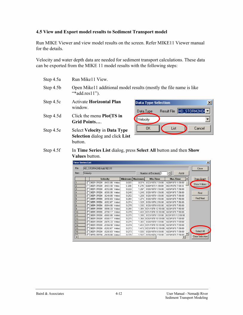
4.5 View and Export model results to Sediment Transport model

Run MIKE Viewer and view model results on the screen. Refer MIKE11 Viewer manual for the details.

Velocity and water depth data are needed for sediment transport calculations. These data can be exported from the MIKE 11 model results with the following steps:

Step 4.5a Run Mike11 View.

Step 4.5b Open Mike11 additional model results (mostly the file name is like “*add.res11”).

Step 4.5c Activate Horizontal Planwindow.

Step 4.5d Click the menu Plot|TS in Grid Points….

Step 4.5e Select Velocity in Data Type Selection dialog and click Listbutton.

Step 4.5f In Time Series List dialog, press Select All button and then ShowValues button.


Step 4.5g In Time Series Value dialog, click the most left-top cell to select all data in the table and copy data into clipboard.

Step 4.5h Run MS-Excel and open a file named as “*-Pull Velocity and Depth or GIS.xls”.

Step 4.5i Select “Row Velocity” Sheet, click “A5” cell and paste.

Step 4.5j Go back Mike11 Viewer, close Time Series Values dialog and TimeSeries List dialog.

Step 4.5k Repeat Step 4.2.5c and 4.2.5d, and select Radius in Data Type Selection dialog and click List button.

Step 4.5l Repeat Step 4.2.5f and 4.2.5g.

Step 4.5m Go back to MS-Excel, select “Row Depth” sheet, click “A4” cell and paste (Ctrl+V).

Step 4.5n Press Ctrl+g to run Save_Data_Gis Macro. Two files will be created with the name “Velocity_GIS.txt” and “Depth_GIS.txt” in the current directory.

Step 4.5o Close Excel.

Step 4.5p Go back to MIKE11 Viewer and close it.

User Manual - Nemadji RiverSediment Transport Modeling


5. SEDIMENT LOADING MODEL

This chapter describes the ArcView 3.x extension that processes MIKE 11 output files, and calculates valley wall erosion based on Creek valley segments as defined by the user.For each valley segment, calculations of erosion volume, vertical erosion, cumulative vertical erosion, and cumulative spatial erosion volume are tabulated. For a conceptual overview, refer to the foldout Figure 5.5 at the back of this chapter

5.1 LOADING THE EXTENSION

All the functionality of this extension is encapsulated in one Extension File. To load the extension, copy the extension file (MIKE11POSTPRO.AVX) to the ArcView extensions folder (\ARCVIEW\EXT32\). Start ArcView and using the command File > Extensions,add MIKE11 POSTPRO.

5.2 INPUTS

This extension combines information from three different sources: data from MIKE11, data from ArcView shapefiles, and inputs from the user.

This extension provides post processing of Mike11 Velocity and Depth output files. The structure of the Mike11 output files is quite simple: tab delimited with columns representing different points (cells) along the stream network, and rows representing different time periods. The user must manually create these files by simply copying the raw data from within MIKE11 and pasting into an Excel spreadsheet.

In Excel, use the SAVE_DATA_GIS macro as described in step 3.2.5n of chapter 4. This macro will convert the data into a GIS compatible format as follows: columns represent spatial variations, rows represent temporal variation; the first column indicates the time step; the second column indicates the elapsed time; and the first row identifies the river chainage or valley segment identification. This first row should contain the 'key' identifier for each cell that corresponds to values in an attribute field in a polygon theme.

Inspect the output text files and ensure that they do not contain any trailing blank lines at the end of the file. These lines must be deleted in order for the ArcView extension to function properly.



This extension also requires a polygon shapefile corresponding to the MIKE11 calculation points along the stream network. For each point, a polygon is delineated that extends to the top of the stream valley walls. These polygons will form the basis for calculatingerosion volumes. Each polygon should be uniquely identified with an attribute field identifying a corresponding MIKE11 calculation point. This polygon shapefile should also have its area geometry calculated in square meters and stored in an attribute field called “AREA”.

Figure 5.1: Stream Valley Walls, MIKE11 polygons defined to match model results.

The user will be prompted to identify values for Roughness, Critical Shear Stress, and Factor Relating Erosion to Shear Stress (Figure 5.2). Default values for each will be suggested.



5.3 USING THE EXTENSION

Once loaded, the extension is launched from a MIKE11 PostPro button on the View button bar. For the button to be available, the view must contain a polygon coverage

representing stream valley polygons corresponding to the MIKE11 calculation points.

This extension also calculates the spatial (downstream) cumulative erosion volume (the total volume of sediment that will pass by any point along the stream). For this function to work, the stream valley polygon theme must contain an attribute field that identifies the polygon’s corresponding ‘DRAINS_TO’ polygon. One special polygon is the river mouth polygon which identifies ITSELF as the ‘drains to’ polygon. All other polygons will drain to another polygon as identified in the ‘DRAINS_TO’ field.

In the view window, with the valley polygon theme selected, click on the MIKE11 PostPro button on the button bar on the top of the ArcView screen. ArcView will display an information box, and then prompt the user to enter values for three variables: Roughness, Critical Shear Stress, Factor Relation Erosion to Shear Stress, and Bluff Slumping Factor. Default values are presented for each: 0.0025, 4, 0.1, and 0.002, respectively.



Figure 5.2Variable Input Dialog Box

Roughness describes how the unevenness of the bed slows the flow of water above the bed.

Critical Shear Stress is the shear stress at which erosion of sediment is just initiated. It has been determined through an in-house Baird database from experimental tests and calibration.

Factor Relating Erosion to Shear Stress describes how the rate of erosion changes with shear stress. This parameter has also been determined through an in-house Baird database from experimental tests and calibration.

Bluff Slumping Factor relates the erosion forces of the stream to the area of the valley polygons defined by the user. This parameter represents the ratio of stream erosion area to the total area of the valley polygon and has been calibrated for the Deer Creek subwatershed.

More discussion on the derivation and influence of these parameters is presented in the accompanying report

Next, the user is presented with a list of all the attribute fields for the valley polygon theme, and asked to select the ‘KEY’ field.The KEY field uniquely identifies each polygon and corresponds to the MIKE11 calculation points identified in the MIKE11 output files for depth and velocity.



After selecting the ‘KEY’ field, the user is prompted to select the MIKE11 depth table file and the velocity table file. These files should be tab delimited.

The user is then prompted to select a base name for the output tables that will be generated. These five output tables are:

• Shear Stress (BaseName_ShearStress.txt);

• Erosion Volume (BaseName_ErosionVolume.txt);

• Cumulative Erosion Volume (BaseName_CumulativeErosionVolume.txt);

• Vertical Erosion (BaseName_VerticalErosion.txt; and

• Cumulative Vertical Erosion (BaseName_CumulativeVerticalErosion.txt).

Shear Stress describes the force of the flow exerted on the river bed.

SHEAR STRESS = 1000 * ( SHEAR VELOCITY ) * ( SHEAR VELOCITY )

where SHEAR VELOCITY = VELOCITY / ( 2.5 * LOG ( 2.5 * DEPTH / ROUGHNESS ) )

Erosion Volume describes volume of sediment eroded from a given area of the bed over a given period of time.

EROSION VOLUME = EROSION RATE * TIME PERIOD * AREA

where EROSION RATE = ( SHEAR STRESS - CRITICAL SHEAR STRESS ) * ( FACTOR RELATING EROSION TO SHEAR STRESS )

Cumulative Erosion Volume tracks the accumulated erosion volume over a given time period (measured as cubic meters).



Vertical Erosion describes the lowering of the bed at any given location for a given time step (measured as millimetres).

Cumulative Vertical Erosion describes the lowering of the bed accumulated over a period of time (measured as millimetres).

Lastly, spatial (downstream) cumulative erosion for each cell (polygon) is calculated. To provide this functionality, the user is prompted to identify two attribute fields within the valley polygon theme: the cumulative vertical erosion field, and the “DrainsTo” field.

Figure 5.4This image illustrates the (downstream) cumulative spatial erosion volume over time shown as extruded areas, based on valley polygon boundaries.


6. ASSESSING LAND USE CHANGE

6.1 Introduction

The NSTM system can assess the impacts of land use changes on sediment load in the river. The CN values are adjusted with the land use change for agriculture practices. The change of CN values affects the peak response time and peak flow in the RR model simulation and then affects on flow velocity and water depth in the HD model simulation. This causes the change of sediment load in rivers. For instance, harvesting the forested land increases CN value resulting in the quicker peak response time, higher peak flow, and larger sediment load. This section describes how to assess the impacts of land use change on runoff, peak flow and sediment load.

6.2 Input

Data input to GIS component:

• Polygons to describe the areas for land use plan.

Data needed in this operations:• MIKE 11 simulation project data;• Rainfall-runoff model parameters;

6.3 Output

• Peak flows;• Runoff volumes;• Discharge in time series;• Water depth in time series;• Flow velocity in time series;• Sediment erosion volume;• Sediment load;

6.4 Operations

a) Draw polygons in which the land use will be changed;

b) Select polygons in Intersect B which are contained in the polygons drawn in step a;

c) Change “Landuse” fields of the selected polygons to a designed land use classification;


d) Follow the instructions in Section 3.4.2 to 3.4.5 to generate new CN values.

e) Change CN values in RR model parameters as described in Section 4.2;

f) Run model as described in Section 4.4;

g) Export flow velocity and water depth to sediment loading model as described in Section 4.5;

h) Run sediment loading model in ArcView GIS to generate the erosion volume and total sediment load.

Documents

USER MANUAL - cdn.cloud1.cemah.net · • Microsoft Windows 9x/NT/2000 Operating System; ... Baird & Associates 1-4 User Manual - Nemadji River Sediment Transport Modeling 1.4 Hardware