Embed Size (px)
Citation preview


Usefulness of High School Average and ACT Scores in Making College Admission Decisions
Richard Sawyer

Abstract
Ample correlational evidence indicates that high school GPA is usually better than
admission test scores in predicting first-year college GPA, although test scores have incremental
predictive validity. Many people conclude that this correlational evidence translates directly to
usefulness in making admission decisions. The issue of usefulness is more complex than is
implied by correlations or by other regression statistics, however.
This paper considers two common goals in college admission: maximizing academic
success and accurately identifying potentially successful applicants. The usefulness of selection
variables in achieving these goals depends not only on the predictive strength of the selection
variables (such as measured by correlations), but also on other factors, including the distribution
of the selection variables in the applicant population, institutions’ selectivity, and their criteria
for what constitutes success. This paper considers indicators of usefulness in achieving
admission goals, and presents estimates of the indicators based on data from a large sample of
four-year institutions.
The results suggest that high school GPA is more useful than admission test scores in
situations involving low selectivity in admissions and minimal to average academic performance
in college. In contrast, test scores are more useful than high school GPA in situations involving
high selectivity and high academic performance. In nearly all contexts, test scores have
incremental usefulness beyond high school GPA.
The paper also presents evidence for two other interesting phenomena: Students use their
high school GPAs and test scores to select the institutions they want to attend, and this self-
selection may be more important than institutions’ selection in admissions. Moreover, high
school GPA by test score interactions are important in predicting academic success.
ii

Acknowledgments
The author thanks Jeff Allen, Julie Noble, and Nancy Petersen for their helpful comments
and suggestions on earlier drafts of this report.
iii

Usefulness of High School Average and ACT Scores in Making College Admission Decisions
Conventional wisdom supported by ample evidence holds that high school grades are
usually better than college admission test scores in predicting first-year college GPA, but test
scores have incremental predictive validity. For example, Morgan (1989) calculated correlations
of high school rank, high school grades, and SAT scores with first-year college GPA in a study
encompassing the academic years 1976 – 1985. Over this time span, multiple correlations for
high school rank and grades ranged from .48 to .52. These correlations were .06 to .14 higher
than the corresponding multiple correlations for SAT scores, but were .05 to .07 lower than the
corresponding multiple correlations for the high school and test score variables jointly. More
recently, Kobrin, Patterson, Shaw, Mattern, and Barbuti (2008) reported correlations of .36 for
high school GPA, .35 for SAT scores, and .46 for high school GPA and SAT scores jointly.
Evidence for ACT scores (1999, 2008c) is similar: For the academic years 1970-1971 through
2006-2007, multiple correlations of high school subject-area grade averages with first-year
college GPA ranged from .48 to .51. The high school grade average correlations were .01 lower
to .08 higher than the corresponding ACT score correlations, and were .04 to .09 lower than the
corresponding correlations for ACT scores and high school grades jointly.
A plausible explanation of these results is that test publishers strive to make test scores
direct measures of cognitive ability only. High school grades, in contrast, are composite
measures of both cognitive ability and academically relevant behavior such as attendance,
punctuality in turning in assignments, and participation in class (Stiggins, Frisbie, & Griswold,
1989; Brookhart, 1993; Cizek, Fitzgerald, & Rachor, 1995/1996; Noble, Roberts, & Sawyer,
2006). College grades are also composite measures of cognitive ability and academically
relevant behavior (Allen, Robbins, Casillas, & Oh, 2008). For this reason, high school GPA

2
should more strongly predict first-year college GPA than test scores do. Weighing in on the
other side, test scores are standardized measures, but high school GPA is not; and test scores
have higher reliability (Allen et al., 2008). On balance, high school GPA comes out somewhat
higher than test scores in its correlation with first-year college GPA, but test scores have
incremental predictive validity.
From this evidence, one might conclude that high school grades are more useful than test
scores in making admission decisions, but that test scores have incremental usefulness. This
conclusion, however, is oversimplified. As will be discussed below, the usefulness of a selection
variable for admission to college does depend in large part on its predictive power, but it also
depends on admission officers’ goals. Correlations are related to the variance in an outcome
variable that is explained by predictor variables. Admission officers, however, are not typically
interested in explaining variance: They are interested in achieving their institutions’ larger goals
to educate students successfully. Usefulness also depends on other statistical issues, such as
utility, applicant self-selection, and institution selectivity. In this paper, I show that the issue of
usefulness is more complex and more interesting than is implied by correlations or other
regression statistics. I show that in many cases, the conventional wisdom based on correlations
does apply to usefulness, but that in some important respects, it does not.
This study is anchored in the current environment of admission, in which applicants to
most four-year institutions must provide scores on admission tests. A broader analysis of the
usefulness of test scores in admission would need to consider what would occur if test scores
were not used. It is very likely that in an admission system without test scores, high school
grades would be subject to inflationary pressure, thereby eroding their predictive power and,
ultimately, their usefulness in achieving institutions’ goals. This paper does not attempt to

3
model the effects of inflation in high school grades in a hypothetical environment either without
college admission tests or with tests optional. There is considerable evidence, however, that
even in the current environment, high school grades are subject to inflation (Woodruff &
Ziomek, 2004; Geisinger, 2009).
Admission Goals
To gauge the usefulness of a selection variable in achieving a goal, we need to specify the
goal. Two common goals related to academic achievement are:
• To maximize academic success among enrolled students.
• To identify accurately those applicants who could benefit from attending the
institution, and to enroll as many of them as possible.
These goals seem similar, but they are not identical. As will be described below, the first
goal is related to the proportion of applicants who would succeed academically if they enrolled
(success rate). The second goal is related to the proportion of applicants whom an institution
correctly identifies as likely to succeed or likely to fail (accuracy rate). Both goals, however,
pertain only to institutions with some degree of selectivity in their admission policies, rather than
to institutions with open admission policies.
The admission selection strategy for accomplishing the first goal is relatively
straightforward: So long as there is a positive relationship between the selection variable and the
success criterion, an institution can increase the success rate of its enrolled students by admitting
only applicants with the highest values of the selection variable. Highly selective institutions can
easily pursue this goal because they typically have many more academically qualified applicants
than they can admit. Less academically qualified students tend not to apply to these institutions
to begin with; these potential applicants in effect select themselves out of the applicant pools. As
4
a result, variance in the predictors is restricted at these institutions, typically resulting in smaller
regression slopes and predictive correlations than at less selective institutions (see, for example,
Kobrin & Patterson, 2010).
All institutions would ideally like to maximize academic success among their enrolled
students. Publicly supported institutions, regional institutions, and other institutions that are
moderately selective also consider the second goal to be important, however. These institutions’
mission is to educate a broad portion of the population, not just the most academically able. A
principal goal in their admission decision making, therefore, is to distinguish between applicants
who are likely to be successful from those who are not likely to be successful. This goal is more
difficult to achieve than the first, because it depends not only on maximizing academic success
among enrolled students, but also on making sure that applicants who are denied admission
would have had little chance of succeeding if they had enrolled. As will be shown later, it is
possible that a selection variable can achieve the first goal (maximizing academic success), but
not the second goal (accurately identifying potentially successful applicants).
Of course, institutions also use test scores in admission for reasons other than achieving
these two goals. One reason is objectivity: to include in their decision making a component that
can be interpreted the same way for all applicants.1 Other potential reasons are to abet
recruitment, to make course placement decisions, to support counseling and guidance services, to
make scholarship decisions, and to assemble data for self-study or comparison to other
institutions (Breland, Maxey, Gernand, Cumming, & Trapani, 2002). At less selective
1 In principle, an institution could statistically adjust high school GPA for high school effects (such as in a hierarchical model), thereby making it more standardized. The practical benefits of doing this are limited, however, if admission test scores are also used (Willingham, 2005).

5
institutions, these other reasons (especially course placement) might be as important as
admission selection.
Institutions’ admission goals also relate to considerations other than future academic
achievement (Camara, 2005). Examples of non-academic goals include assembling a student
body with non-academic achievements, promoting cultural diversity, and promoting support
from alumni. For this reason, test scores, high school course work, and high school grades are
only part of institutions’ admission decision making. Most institutions, in fact, make admission
decisions using a holistic approach, rather than by an explicit formula (Breland et al., 2002).
Laird (2005) further advocated a holistic individualized approach, in which institutions “make
careful, individual decisions about each applicant based on the information at hand and the
professional judgment of the admissions staff.”
Student Self-Selection
This paper presents evidence that students use high school GPA and test scores in
deciding on the institutions to which they apply for admission. Moreover, students’ self-
selection on these variables in applying to college is likely as important as institutions’ reliance
on these variables in making admission decisions. Therefore, high school grades and test scores
contribute both directly and indirectly to attaining the goal of academic success.
Institutions’ goals in making admission decisions overlap to some extent with those of
prospective applicants. With respect to the first goal, for example, most students want to succeed
academically. Therefore, the success rates associated with particular values of high school GPA
and test scores are as relevant to students in their decision making as they are to institutions.
Communicating usefulness in terms of success rates instead of correlations is likely to be more
meaningful to students, just as it is to institutions.

6
Academic Success
In this paper, academic success is defined jointly by retention through the first year and
by overall first-year college GPA (FYGPA). Other researchers (e.g., Saupe & Curs, 2008 and
Bowen, Chingos, & McPherson, 2009) have studied long-term academic success (degree
completion and cumulative GPA). Long-term success is clearly an important goal for all
institutions. Attaining this goal through admission selection, however, is likely to be more
feasible at highly selective institutions that attract and enroll only the most academically
qualified applicants than at institutions whose mission is to educate a broad segment of students
with diverse academic skills. At highly selective institutions, graduation rates and cumulative
GPAs are typically very high, and many more highly qualified students apply than can be
admitted. At less selective institutions, grades during the first year strongly mediate predictions
of long-term success based on pre-enrollment measures (Allen et al., 2008). To achieve their
goals, these institutions select applicants who have a reasonable chance of succeeding in the first
year, given the interventions (e.g., counseling and course placement) that the institutions might
provide.
For the analyses in this paper, students who complete the first year with a given level or
higher of FYGPA are considered to be successful (S=1); otherwise, they are considered to be
unsuccessful (S=0). Although dichotomizing a quasi-interval variable such as FYGPA degrades
information in a statistical sense, dichotomies correspond more closely to admission officers’
interpretations: Are a college student's grades high enough at least to get by, or has the student
performed well? Moreover, as will become apparent, the usefulness of high school GPA and
test scores depends strongly on which level of success one considers.

7
The analyses in this paper consider four levels of success:
* S20: Retention through first year, and 2.0 or higher FYGPA (minimal success)
* S30: Retention through first year, and 3.0 or higher FYGPA (typical level of
success)
* S35: Retention through first year, and 3.5 or higher FYGPA (high level of success)
* S37: Retention through first year, and 3.7 or higher FYGPA (very high level of
success)
By these criteria, students who either drop out or have a low FYGPA during their first year are
unsuccessful. In the data on which this study is based, about 84% of students were at least
minimally successful, about 52% were at least typically successful, about 27% were highly
successful, and about 16% were very highly successful.
Target Population and Indicators of Usefulness
Admission selection rules are applied to applicants. Therefore, a common-sense
indicator of the usefulness of particular selection rules is the estimated proportion of applicants
for whom the admission goals would be achieved if they enrolled (Sawyer, 2007). For
institutions whose goal is to select the applicants who are most likely to be successful, this
proportion is the estimated success rate:
Nc
pcSR Nci
i
)1(
ˆ)(
)(
−=
∑≥ (1)
= estimated proportion of applicants who, if enrolled, would be successful.
Here, are the ordered estimated conditional probabilities of success of
the N applicants, given one or more selection variable, and 1 - c is equal to the proportion of
applicants selected. I refer to the variable c as the “cutoff proportion”; it is equal to the
)()()1( ˆˆˆ Ni ppp ≤≤

8
cumulative relative frequency associated with a value of the selection variable. The variable c
relates to an institution’s selectivity in admission; the variable SR(c) is the estimated success rate
among the students the institution does admit.
An institution serving a high-risk population might be concerned about minimizing the
proportion of academic failure and near-failure (Fs and Ds) among its first-year students; it
would consider SR for the S20 criterion. An institution with few academic failures might instead
be interested in maximizing the proportion of students who earn a B or higher average (S30
criterion). A highly selective institution that expects most of its students to attain excellent
academic achievement might consider SR for the S35 or S37 criteria. Alternatively, an institution
using high school grades and test scores for merit scholarship selection, rather than admission,
might also consider SR for the S35 or S37 criteria.
For institutions whose goal is accurately to identify potentially successful applicants, the
relevant indicator is the estimated accuracy rate:
N
ppcAR Nci
icNi
i ∑∑≥<
+−=
)()( ˆ]ˆ1[)( (2)
= proportion of applicants for whom a correct admission decision is made.
The AR indicator corresponds to an expected utility in which admitting an applicant who
would be successful and denying admission to an applicant who would be unsuccessful are both
weighted 1, and admitting an applicant who would be unsuccessful and denying admission to an
applicant who would be successful are both weighted 0. The AR indicator can be generalized to
other utilities by assigning different weights to the four outcomes (Sawyer, 1996). For example,
if an institution believes that admitting students who do not succeed is less serious an error than

9
denying admission to students who would have been successful, then it could assign a larger
weight to the former outcome than to the latter.
An institution concerned about accurately identifying students who could benefit from
attending the institution might consider AR for the S30 criterion. A highly selective institution
that expects excellent performance from its students, but that is concerned about denying
admission to students who might perform at a high level, might consider AR for the S35 or S37
criteria.
Note that both indicators pertain to the target population of applicants, as a whole or in
part, rather than only to enrolled students. The indicator AR(c) pertains to the entire applicant
population for an institution, whereas SR(c) pertains to the subset of applicants who meet the
institution’s cutoff proportion. Predictive validity studies that only summarize correlations and
other regression statistics based on data of enrolled students overlook this point. On the other
hand, even though the indicators in Equations (1) and (2) pertain to all applicants, we must
estimate their conditional probability of success component from the data of enrolled students:
The reason is that we can obtain outcome data only from applicants who enroll at an institution.
Institutions are unlikely to forego using high school GPA and test scores in making
admission decisions solely to do research.2 We therefore need to make additional assumptions
about the conditional probability of success components in the indicators. With the dichotomous
success criterion S considered here, we assume that the conditional probability of success, given
the selection variable(s) X, is the same for the non-enrolled applicants as for the enrolled
students:
p(x) = P[S=1 | X=x, non-enrolled] = P[S=1 | X =x, enrolled]
2 Although some non-open-enrollment institutions have test-score-optional admission policies, most of them continue to use test scores, at least for some applicants (Breland et al., 2002). Furthermore, it is doubtful that any institution disregards high school GPA (or its transformation to high school rank) in its admission decisions.

10
This assumption is analogous to that for the traditional adjustment of correlations for
restriction of range, which requires that the applicant and enrolled student groups have the same
conditional mean and variance functions (e.g., Lord & Novick, 1968). Although empirically
testing the correctness of this assumption is not feasible, one could investigate the robustness of
the indicators of usefulness to specified departures from the assumption.
With this assumption, calculating the indicators is straightforward: Simply score the
entire applicant population with the fitted conditional probability of success function (e.g., using
a logistic regression model), and then calculate the indicators from the ordered estimated
conditional probabilities.
Cutoff proportion
Note that the indicators considered here assume that an institution admits the top
proportion 1-c of the applicants, based on their conditional probability of success, and that it
denies admission to the bottom proportion c. Unlike the correlation coefficient, which is a global
measure, the indicators of usefulness described here depend explicitly on c. These indicators, as
well as other considerations (such as capacity for the number of enrolled students), can inform an
institution’s choice of c.
Of course, institutions do not use simple cutoffs in making admission decisions. As is
noted in the discussion following Table 4, institutions likely use high school grades and test
scores as initial screens, but base their final admission decisions by considering additional
variables. Equations (1) and (2) are mathematical idealizations that enable us to compare the
properties of alternative selection variables. In this paper, cutoff proportions range from .01
(virtually all applicants admitted) to .99 (extreme selectivity).

11
Correlation Coefficient
According to (1) and (2), the indicators SR(c) and AR(c) are functions of the conditional
probability of success p(x), the distribution of p(x) in the applicant population, and the cutoff
proportion c. If the selection variable X and the underlying outcome variable Y have a bivariate
normal distribution in the applicant population, then we can more directly calculate SR(c) and
AR(c) by integrating the bivariate normal density function over appropriate regions of X and Y:
c
dydxyxcSR S cz z
−=∫ ∫∞ ∞
1
);,()(
ρφ
,);,();,()( ∫ ∫∫ ∫∞ ∞
∞− ∞−+=
S c
S c
z z
z zdydxyxdydxyxcAR ρφρφ (3)
where is the value of a standard normal variable corresponding to the cutoff proportion c on
the selection variable X,
cz
YYSS yz σμ /)( −= is the value of a standard normal variable
corresponding to the success level on the outcome variable Y, andSy φ is the bivariate standard
normal density function with correlation parameter ρ .
A possible reason why researchers often interpret ρ as a measure of effectiveness in
selection is that given a bivariate normal distribution, SR and AR depend on ρ . As is clear from
(3), however, SR and AR also depend on the success variable S and the cutoff proportion c, as
well as on ρ . Moreover, as we shall soon see, the assumption of bivariate normality is not
tenable in the context of college admission selection. In particular, high school GPA has a
severe negative skew and a pronounced ceiling.
Incremental Usefulness
A basic question that we should ask when evaluating the usefulness of a selection
variable X is: Does using a variable X for selection increase the success rate and the accuracy

12
rate over what would result if an institution did not use X (i.e., if it admitted all applicants or
denied admission to all applicants)? Admitting all applicants amounts to setting c=0 in
Equations (1) and (2); the resulting quantity for either indicator is the base success rate
,N
p̂)(AR)(SRBSR iall
)i(∑=== 00 (4)
which is also equal to the overall (marginal) probability of success. Denying admission to all
applicants amounts to setting c=1, and would result in an accuracy rate of 1-BSR. I refer to
admitting all applicants and denying admission to all applicants as “null decisions.”
Note that SR depends on both the conditional probability of success function p and on the
distribution of p (or, alternatively, of X) in the applicant population. Nevertheless, if p is an
increasing function of x (the value of the selection variable X), then SR is also an increasing
function of x (see Appendix), and therefore of c. Hence, if p is an increasing function of X, SR(c)
exceeds BSR. Incremental usefulness in terms of success rate therefore corresponds to the
traditional notion of nonzero regression slope or correlation.
As we shall see, however, the same need not be true of AR: Even though a variable is
positively related to success, using it in selection might result in a decrease in classification
accuracy. One can show by a straightforward differentiation argument (see Appendix) that
AR(c) exceeds both BSR and 1-BSR at some cutoff proportion if, and only if, the conditional
probability of success function p(x) crosses 0.5. Moreover, AR(c) achieves its maximum value at
the cutoff proportion c′ associated with x′ (and this maximum exceeds BSR and 1-BSR) if, and
only if, . 5.0)( =′xp
Another important question involves comparing alternative selection variables X and W:
Does using X and W jointly increase the success rate and accuracy rate over that which would

13
occur if we used X only? This question pertains to incremental usefulness, and is analogous to
the traditional notion of incremental predictive validity.
Because SR(c) and AR(c) depend on the cutoff proportion c, the answers to both
questions can vary, depending on c. A selection variable might have incremental usefulness
(either with respect to null decisions or with respect to another selection variable) at some cutoff
proportions, but not at others.
Data
The analyses in this paper are based on data from 192 four-year postsecondary
institutions that use ACT scores in their admission procedures (ACT, 2008a). The institutions
provided outcome data either through their participation in ACT’s predictive validity service or
through participation in special research projects. The outcome data pertain to the following
entering freshman class years: 2003 (1% of institutions), 2004 (31%), 2005 (68%), and 2006
(1%). For institutions that had data from more than one entering freshman class, I used the most
recent data.
Institutional characteristics. Table 1 compares characteristics of the 192 institutions in
the sample to those of all four-year institutions in the U.S. (ACT, 2008b). The sample
institutions are broadly representative of four-year institutions in the U.S. with respect to their
proportion of minority students and students’ average ACT Composite scores. A majority of the
institutions in this study are public, however, whereas only about 30% of all postsecondary
institutions are public. Moreover, the institutions in this study tend to be much larger than four-
year institutions generally.

14
TABLE 1
Summary of Institutions in Sample and of Four-Year Institutions in the U.S.
Characteristic
Sample (N=192)
Four-year institutions in the U.S. (N=2,044)
Affiliation: Proportion public .57 .30
Self-reported admission selectivity: Proportion selective or highly selective
.27
.30
Median undergraduate enrollment 2,883 1,545
Median proportion minority .21 .25
Median average ACT Composite score of enrolled students
21.8
22.0
When students register to take the ACT, they report their high school course work and
grades. The analyses are based on HSAvg, the average of students’ self-reported grades in
standard college-preparatory courses, and on ACT-C, the Composite (average) of students’ ACT
scores in English, mathematics, reading, and science. The outcome success variables S20, S30,
S35, and S37, are based on data reported by the postsecondary institutions.
Student characteristics (pooled sample). Table 2 contains the means and standard
deviations of the pre-enrollment and outcome measures in the pooled sample of 120,338 students
across all institutions.

15
TABLE 2
Summary of Enrolled Student Characteristics (Pooled Sample; N=120,338)
Characteristic
Mean
SD
Pre-enrollment measures HSAvg 3.42 0.50 ACT-C 22.6 4.3 Outcome measures S20 0.84 0.37 S30 0.52 0.50 S35 0.27 0.44 S37 0.16 0.37 FYGPA 2.78 0.95
As was noted previously, SR and AR are functions of the correlation ρ (and of other
properties of the selection and outcome variables) when they have a bivariate normal
distribution. Figure 1 shows histograms of HSAvg, ACT-C, and FYGPA standardized to z-scores
with respect to the enrolled student population pooled over institutions. Figure 1 also shows a
reference curve for the standard normal distribution.

16
FIGURE 1. Distributions of Standardized FYGPA, HSAvg, and ACT-C, Compared to the Standard Normal Distribution
0
5
10
15
20
25
30
-3.5 -3 -2.5 -2 -1.5 -1 -0.5 0 0.5 1 1.5 2 2.5 3 3.5Interval of standardized variable
Perc
ent i
n in
terv
al
0
5
10
15
20
25
30-3.75 -2.75 -1.75 -0.75 0.25 1.25 2.25 3.25
FYGPA
HSAvg
ACT_C
Normal
FYGPA 0.0 0.9 1.8 2.8 3.7 HSAvg 2.4 2.9 3.4 3.9
ACT-C 14 18 22 27 31 35
Value on original scale

17
As is clear from the marginal distributions shown in Figure 1, the assumption of bivariate
normality is untenable. The distribution of HSAvg in our data has a pronounced negative skew
(-0.9). The modal category of HSAvg is its maximum category, 0.75 to 1.25 standard deviations
above the mean. HSAvg is also negatively skewed in broader populations: (-0.7) combined score
sender / enrolled student population; (-0.7) all 2005 ACT-tested high school graduates; and (-0.4)
a nationally representative sample of eleventh-grade students (Casillas, Robbins, Allen, Kuo,
Hanson, & Schmeiser, 2010).
FYGPA is also negatively skewed (-1.1), and has a minor mode at its minimum category
(2.75 to 3.25 standard deviations below the mean). The distribution of ACT-C is more nearly
symmetric (skewness = 0.1). Furthermore, both the conditional mean of FYGPA, given HSAvg,
and the conditional mean of FYGPA, given ACT-C, are slightly curvilinear (not shown in Figure
1). Therefore, one should be cautious in applying normal theory to calculate SR and AR.
Distribution of enrolled student characteristics among institutions. Table 3 summarizes
the distribution of the means and correlations of the pre-enrollment and outcome variables
among institutions.

18
TABLE 3
Summary of Enrolled Student Characteristics Among Institutions
(N=192)
Characteristic
Median
Min. – Max.
Number of ACT-tested enrolled students 319 16 – 5,210 Pre-enrollment measures HSAvg mean 3.36 2.49 – 3.80 ACT-C mean 21.8 14.9 – 28.7 Outcome measures S20 mean 0.84 0.33 – 1.00 S30 mean 0.49 0.01 – 0.96 S35 mean 0.23 0.01 – 0.71 S37 mean 0.14 0.00 – 0.44 FYGPA mean 2.83 1.76 – 3.58 Correlations HSAvg / ACT-C correlation 0.44 -0.01 – 0.66 FYGPA / HSAvg correlation 0.48 -0.14 – 0.83 FYGPA / ACT-C correlation 0.41 -0.15 – 0.63 FYGPA / HSAvg & ACT-C multiple R 0.54 0.06 – 0.84
Pre-enrollment measures. The median mean HSAvg over the institutions in the sample
(3.36) is similar to the mean HSAvg (3.32) of first-year college students nationally. The median
mean ACT-C score over the institutions in the sample (21.8) is also similar to the mean score
(22.1) of first-year college students nationally in 2008 (ACT, 2009a).
Outcome measures. At typical institutions in the sample, a huge majority (84%) of
students completed the first year with at least a C average, and nearly half completed the first
year with a B or higher average. Only a small proportion of students had FYGPAs of 3.7 or

19
higher. The median average FYGPA of 2.83 reflects a minor mode in the FYGPA distribution at
the value 0.0 (3% of students).
Among 1,634 institutions that recently completed a questionnaire administered by ACT,
the average self-reported retention rate was 73% (ACT, 2009b). The 73% result was based on a
different definition of retention (re-enrollment in the sophomore year) than that in this study
(completion of the first year), but it suggests that the institutions in this study have higher
retention rates than institutions generally.
Correlations. The median correlations at the bottom of Table 3 show the typical result:
HSAvg is a better predictor of FYGPA than ACT-C, but ACT-C has incremental predictive
validity. Of more interest is the huge variation among institutions in their correlations. At two
institutions, HSAvg and ACT-C were both negatively correlated with FYGPA. None of the
correlations were statistically significant (p < .05), even though neither institution’s sample size
was small (N=145 and 154). At the other extreme, HSAvg and ACT-C jointly accounted for
nearly two-thirds of the variance in FYGPA (multiple R = .83 and .84) at two other institutions.
Although not shown in Table 3, correlations for both predictor variables were higher at private
institutions, at institutions with smaller percentages of minority students, and at institutions with
larger standard deviations in the predictor variables. Correlations were lower at highly selective
institutions.
Applicants and Score Senders
As was previously noted, postsecondary institutions make admission decisions about
applicants; therefore, indicators of usefulness should be calculated for this target population. For
several reasons, it is not feasible in a study involving many institutions to identify their
applicants. I instead used score senders (students who sent their ACT scores to particular

20
institutions) as a proxy for applicants. Score senders can be thought of as predecessors to
applicants: Not all score senders decide to apply to an institution, but most applicants will have
sent their scores.3 The 192 institutions in the sample for this study had 483,451 non-enrolled
score senders, in addition to their 120,338 enrolled students. Strictly speaking, therefore, the
results reported here pertain to score senders, rather than to actual applicants.
Fifty-three of the 192 institutions represented in the study provided data on their actual
applicants. By matching the applicant, score-sender, and enrolled student files of the 53
institutions, I determined whether an individual was a non-applicant, non-enrolled score sender,
a non-enrolled applicant, or an enrolled student. Table 4 below compares the distributions of
HSAvg and ACT-C among these three groups:
TABLE 4
Distribution of HSAvg and ACT-C, by Application and Enrollment Status
at 53 Institutions
Application/enrollment status
N
HSAvg Mean (SD)
ACT-C Mean (SD)
1. Non-applicant, non-enrolled
score senders 179,185 3.23 (0.59) 21.3 (4.4)
2. Non-enrolled applicants 17,305 3.40 (0.51) 22.3 (4.0) 3. Enrolled students 85,899 3.43 (0.48) 23.0 (4.1)
Note that the means of both variables increase from non-applicant score senders to non-
enrolled applicants, and from non-enrolled applicants to enrolled students, but the standard
deviations mostly decrease. Moreover, the non-applicant score-sender means and the non-
enrolled applicant means differ more than the non-enrolled applicant means and the enrolled
3 Some institutions permit applicants to submit test scores on their high school transcripts.

21
student means. This result suggests that with respect to HSAvg and ACT-C, applicant self-
selection is at least as important as institutions’ selection through admission decisions.
In terms of standard deviations, the difference between the mean ACT-C score of the non-
enrolled applicants and the enrolled students is only moderately large (0.18 SD). The
corresponding difference in mean HSAvg is quite small (0.06 SD). This result suggests either
that institutions’ admission decisions were based on other variables, in addition to ACT-C and
HSAvg, or that admitted students’ decisions to enroll were based on other variables, or (as seems
likely) both. Although not addressed by these data, one plausible hypothesis is that students and
institutions primarily use high school grades and test scores as initial screens, but base their final
decisions substantially on other variables. Some of these other variables might include
characteristics such as cost, location, personal goals, athletic talent, out-of-class
accomplishments, and previous connections with the institution.
Method
Modeling Probability of Success
According to Equations (1) and (2), an essential component of the indicators SR(c) and
AR(c) is , the estimated conditional probability of success, given the value
of the selection variable X. I estimated the conditional probability of success using a hierarchical
logistic regression model.
]|1[ˆ)( xXSPxp ===
In logistic regression, we model the log-odds ( )])(1)([ln xpxp − , rather than
directly; we can then calculate an estimated p(x) from the estimated log-odds. The
intercept
)(xp
0β and the slope 1β in the log-odds model are related to the point at which the
probability-of-success curve crosses 0.5 and to its slope at this point: 5.0)/( 10 =− ββp , and

22
=−′ )/( 10 ββp 4/1β . Additionally, in the hierarchical model, the intercept and slope coefficients
for the linear predictor of the log-odds vary among institutions:
jj
jj
ijjjij
ij
u
u
xxp
xp
111
000
10)(1)(
ln
+=
+=
+=⎟⎟⎠
⎞⎜⎜⎝
⎛
−
γβ
γβ
ββ
(5)
The intercept j0β for institution j is the sum of a fixed effect 0γ that is constant across
institutions and a random effect that is specific to institution j. Similarly, the slope term ju0 j1β
for institution j is the sum of a fixed effect 1γ that is constant across institutions and a random
effect that is specific to institution j. The symbol refers to a selection variable (either
HSAvg or ACT-C) for student i at institution j. To facilitate interpretation of the intercept, as
well as computation, I centered about its mean across students (grand-mean centering).
ju1 ijx
ijx
The hierarchical model is more precise than a model based on data pooled across
institutions, because it takes into account the dependence of observations within institutions
(Snijders & Bosker, 1999). Furthermore, the hierarchical model is more parsimonious (has
fewer parameters) than estimating a separate model for each of the 192 institutions. As a result,
predictions based on the hierarchical model are likely to be more accurate at small institutions
than predictions based on institution-specific models.
The concentration of HSAvg at its highest values suggests that we might improve
prediction at the high end by a suitable transformation. One possibility is to replace HSAvg with
its cumulative relative frequencies (in effect, causing it to have a more nearly uniform
distribution). Another possibility is to transform HSAvg to have approximately a normal

23
distribution. Although transformations like this can decrease skewness, they do not change the
concentration of the distribution on particular values (e.g., 4.0).
I also estimated models based on HSAvg and ACT-C jointly. A standard way to model
the relationship between probability of success and both variables is to include them as main
effects and in the hierarchical model. It is possible, however, that the relationship
between the log-odds and each selection variable depends on the value of the other selection
variable; we can test this possibility with an interaction term in the following model:
ijx1 ijx2
ijij xx 21
33
222
111
000
21322110)(1)(
ln
γβ
γβ
γβ
γβ
ββββ
=
+=
+=
+=
+++=⎟⎟⎠
⎞⎜⎜⎝
⎛
−
j
jj
jj
jj
ijijjijjijjjij
ij
u
u
u
xxxxxp
xp
(6)
For example, Equation (6) says that the slope of the log-odds on , namelyijx1 ijjj x231 ββ + ,
depends on 4ijx2 . As in Equation (5), I centered all the independent variables about their
respective grand means.
Initially, I estimated the interaction Model (6) using data of all 120,338 students in the
sample. Plots of the fixed effects in this initial model revealed that for values of HSAvg below
2.0, the estimated linear predictor was a weakly decreasing function of ACT-C. I therefore re-
estimated the interaction model using data only for students with HSAvg above 2.0. For the 945
students whose HSAvg was less than 2.0, I set the probability of success equal to their overall
base success rate.
4 I would like to thank Professor Joseph Rodgers, University of Oklahoma, for his suggestion to estimate interaction models.

24
To simplify the extensive data processing required to estimate the hierarchical logistic
models, and to calculate the indicators of usefulness SR(c) and AR(c), I did both using the same
software (SAS). I used PROC NLMIXED (SAS Institute, 2008) to estimate the hierarchical
logistic models. With large data sets, NLMIXED requires gargantuan computer resources, and I
could not use it to estimate a model with a random effect in the interaction term
coefficient
iju3
j3β and with level-2 means as additional fixed effects. I therefore used the simplified
Model (6) to calculate success rates and accuracy rates.
More complex hierarchical models. To learn more about the variation in the coefficients
among institutions, I estimated a more complex model with the HLM6 software (Raudenbush,
Bryk, Cheong, & Congdon, 2004):
js
sjsj
js
sjsj
js
sjsj
js
sjsj
ijijjijjijjjij
ij
uW
uW
uW
uW
xxxxxp
xp
333303
222202
111101
000000
21322110)(1)(
ln
∑
∑
∑
∑
++=
++=
++=
++=
+++=⎟⎟⎠
⎞⎜⎜⎝
⎛
−
γγβ
γγβ
γγβ
γγβ
ββββ
(7)
Potential level-2 predictors for sjsjsjsj WWWW 3210 ,,, ,,,, 3210 jjjj ββββ respectively, were the
institution means jx1 and jx2 of the centered selection variables and , the institutional
mean of the centered interaction term, and the institutional characteristics affiliation
(public/private), undergraduate enrollment, and percentage minority. I estimated models for
which all the student-level fixed effects
ijx1 ijx2
30201000 ,,, γγγγ were statistically significant (p < .001),

25
the fixed effects ssss 3210 ,,, γγγγ for the institution characteristics were
statistically significant (p < .01), and the variances of the random effects were
statistically significant (p < .01). Model (7) tells us whether the coefficients
sjsjsjsj WWWW 3210 ,,,
jjjj uuuu 3210 ,,,
jjjj 3210 ,,, ββββ
vary systematically by the institution characteristics and whether they vary
randomly by institution. I did not use Model (7) to calculate success rates and accuracy rates.
sjsjsjsj WWWW 3210 ,,,
Cross-classified models. Students are nested within high school, as well as within
postsecondary institution. Therefore, the regression coefficients in Equations (5), (6), and (7)
could vary among both high schools and postsecondary institutions, particularly when HSAvg is
the selection variable. Estimating models with cross-classified random effects is difficult,
especially in large data sets, and estimating nonlinear cross-classified models would be more
complex still. I therefore deferred investigating them to a future study.
Indicators of Usefulness
From the estimated probabilities of success returned by NLMIXED for models (5) and
(6), I calculated SR(c) and AR(c) using the cutoff proportions c= .01, .10, .20, .30, .40, .50, .60,
.70, .80, .85, .90, .95, and .99 for each selection variable. These cutoff proportions correspond to
increasing degrees of admission selectivity: The cutoff proportion .01 corresponds to admitting
all but the bottom 1% of students, as ranked by their estimated probability of success; the cutoff
proportion .99 corresponds to admitting only the top 1% of students.
Incremental success rate with respect to base rate. The incremental success rate
associated with a selection variable is the difference between SR(c), the success rate associated
with admitting applicants at or above cutoff proportion c, and the base success rate BSR=SR(0),
the success rate associated with admitting all applicants. Recall that a selection variable has
positive incremental success rate if its probability-of-success curve is increasing. As it turned

26
out, the probability-of-success curves for all four success variables at all 192 institutions were
increasing.5 I calculated for each value of c the median incremental success rate across
institutions:
.})({)(..1921
iBSRciSRmediancSRIncMedi
−=≤≤
(8)
Incremental success rate of ACT-C with respect to HSAvg. As in evaluating correlations,
it is important to determine whether a selection variable is incrementally useful with respect to
another variable. To gauge the incremental usefulness of ACT-C with respect to HSAvg for
maximizing the academic success of enrolled students, I calculated the median difference
between the success rate for the model based on HSAvg and ACT-C jointly, and the success rate
for the single-variable model based on HSAvg only:
{ } . ciSRciSRmediancSRIncMed HSAvg]CACT and HSAvgCACT
i
)()()(.. ][[][
1921
−= −−
≤≤
(9)
Incremental accuracy rate with respect to null decisions. As was noted earlier, a
selection variable has incremental accuracy with respect to the base success rate (BSR)
associated with accepting all applicants and the base failure rate (1-BSR) associated with denying
admission to all applicants if, and only if, its probability-of-success curve crosses 0.5
somewhere. Otherwise, the institution would do better (in terms of accuracy) to choose either
the null decision to accept all applicants or the null decision to reject all applicants. I therefore
calculated:
Rel. Freq. Inc. Acc. = proportion of institutions whose probability-of-success
curve crosses 0.5 somewhere. (10)
5 Because hierarchical models shrink coefficient estimates toward the mean, all estimated slopes were positive, even at the two institutions with negative correlations.

27
This statistic is the proportion of institutions for which AR(c) exceeds max[BSR, 1-BSR] at some
cutoff proportion; it is relevant for evaluating a selection variable globally across values of c.
Note that even if an institution’s probability-of-success curve cross 0.5 at some cutoff
proportion AR(c) need not exceed max[BSR, 1-BSR] at all cutoff proportions. I therefore
calculated for each cutoff proportion c the relative frequency of incremental accuracy among
institutions:
,c′
Rel. Freq. Inc. Acc(c) = proportion of institutions for which ARi(c) - max[BSRi, 1-BSRi] > 0 . (11)
I also calculated the median incremental accuracy rate among the institutions where it is positive:
{ } ,]1,max[)()(...0]1,max[)(:
iBSRiBSRciARmediancARIncMediii BSRBSRcARi
−−=>−−
(12)
This statistic shows the typical improvement in accuracy rate, above admitting or denying
admission to everyone, at institutions where there is any such improvement.
Incremental accuracy rate of ACT-C with respect to HSAvg. To gauge the incremental
usefulness of ACT-C for accurately identifying applicants who could benefit from attending an
institution, I calculated the median difference between the accuracy rate for the model based on
HSAvg and ACT-C jointly, and the accuracy rate for the single-variable model based on HSAvg
only:
{ }.ciARciARmediancARIncMed HSAvgCACT and HSAvgCACT
ii]CACT and HSAvg
i BSRBSRcARi
)()()(.. ][][][
0]1,max[)(: [
−= −−
>−−−
(13)
The median pertains to institutions for which the joint HSAvg and ACT-C model has incremental
accuracy at or above cutoff proportion c.

28
p
Effects associated with extrapolation to score-sender population. Note that the success
rate and accuracy rate statistics depend not only on the cutoff proportion c and the values of the
estimated conditional probability of success function ) , but also on the distribution of p) in the
applicant population. Because applicant data were not available for most institutions in this
study, I used data from score senders. From the previous discussion, we know that score senders
have somewhat lower mean HSAvg and ACT-C than applicants, and that applicants have
somewhat lower mean HSAvg and ACT-C than enrolled students. To obtain a rough notion of
how using the score sender data affected the estimated success rates and accuracy rates, I
recalculated these statistics using only the enrolled student data. If results calculated from the
enrolled student data are similar to the results calculated from the combined group of non-
enrolled score senders and enrolled students, then we can have more confidence that results
calculated from the combined group of non-enrolled applicants and enrolled students would be
similar.
Table 5 on the following page summarizes the simple hierarchical predictive models
(Equations (5) and (6)) for each of the four success levels. Note that in both of the single-
variable models (labeled A and B in Table 5), the fixed effects for the HSAvg and ACT-C slope
coefficients are positive and statistically significant (p < .001). Moreover, the slope coefficients
for HSAvg and ACT-C both increase with success level. For example, the HSAvg slope
coefficient for the 2.0 success level is 1.596; for the 3.7 level, it is 3.759. This result suggests
that HSAvg and ACT-C are more strongly related to high levels of success than they are to low
levels of success.
Hierarchical Models
Results

29
TABLE 5
Simple Hierarchical Models for Predicting Success from HSAvg and ACT-C
Success level Fixed effects 2.0 or higher 3.0 or higher 3.5 or higher 3.7 or higher Model Variable Coefficient p < Coefficient p < Coefficient p < Coefficient p <
A
Intercept HSAvg
2.019 1.596
.001
.001 0.007
2.283 .877 .001
-1.586 3.079
.001
.001 -2.552
3.759 .001 .001
B
Intercept ACT-C
1.974 0.161
.001
.001 0.129
0.232 .004 .001
-1.268 0.271
.001
.001 -2.043
0.295 .001 .001
C
Intercept HSAvg ACT-C HSAvg X ACT-C
2.196 1.539 0.105 0.084
.001
.001
.001
.001
0.185 1.931 0.150 0.097
.001
.001
.001
.001
-1.478 2.386 0.163 0.092
.001
.001
.001
.001
-2.457 2.825 0.173 0.095
.001
.001
.001
.001
Success level Random effects 2.0 or higher 3.0 or higher 3.5 or higher 3.7 or higher Model Variable Std. dev. p < Std. dev. p < Std. dev. p < Std. dev. p <
A
Intercept HSAvg
0.846 0.332
.001
.001 0.642
0.632 .001 .001
0.550 0.866
.001
.001 0.690
1.170 .001 .001
B
Intercept ACT-C
0.788 0.051
.001
.001 0.579
0.056 .001 .001
0.502 0.059
.001
.001 0.562
0.066 .001 .001
C
Intercept HSAvg ACT-C
0.785 0.252 0.030
.001
.004
.004
0.636 0.500 0.033
.001
.001
.001
0.570 0.705 0.036
.001
.001
.001
0.710 0.936 0.041
.001
.001
.001

30
The variances of the HSAvg and ACT-C slope coefficients among institutions (lower half
of Table 5) also increase with success level. The strength of these variables’ relationships with
higher levels of success varies more among institutions than does the strength of their
relationships with lower levels of success.
The coefficients of variation for the HSAvg and ACT-C slopes (the standard deviation of
the slope random effect divided by the slope fixed effect) are approximately 0.2 and 0.3,
respectively. This result indicates that there is moderate variation among institutions in the
slopes of the predictor variables. Nevertheless, the estimated slopes from the hierarchical model
are positive at all institutions.
A typical way to compare the strength of predictor variables is to standardize their slope
coefficients with respect to their standard deviations. On multiplying the fixed effects for the
HSAvg and ACT-C slopes in Table 5 by the corresponding standard deviations in Table 1, we
find that the standardized regression coefficients for HSAvg are uniformly larger than those for
ACT-C. As was previously noted, however, the usefulness of selection variables depends on
other properties, in addition to their regression coefficients. Examining the probability of
success curves, rather than just the slope coefficients, lets us observe differences in strength of
prediction across the entire ranges of predictor variables.
Figures 2 and 3 on the following pages show probabilities of success calculated from the
fixed effects of HSAvg and ACT-C. These probability curves pertain to typical postsecondary
institutions (i.e., those for which the random effects are 0). In both graphs, the horizontal axis is
scaled in terms of both the values of the selection variables and their associated cutoff
proportions (cumulative relative frequencies, c).

31
Figure 2. Probability of Success, Given HSAvg
0
0.1
0.2
0.3
0.4
0.5
0.6
0.7
0.8
0.9
1
1.6 1.8 2.0 2.2 2.4 2.6 2.8 3.0 3.2 3.4 3.6 3.8 4.0
2.0 or higher
Prob
abili
ty o
f suc
cess
3.0 or higher
3.5 or higher 3.7 or higher
HSAvg
.01 .10 .20 .30 .40 .50 .60 .70 .80 .85 .90
Cutoff proportion (cumulative relative frequency) of HSAvg

32
0
0.1
0.2
0.3
0.4
0.5
0.6
0.7
0.8
0.9
1
12 14 16 18 20 22 24 26 28 30 32 34 36ACT-C score
Prob
abili
ty o
f suc
cess
2.0 or higher
3.0 or higher
3.5 or higher
3.7 or higher
.01 .10 .20 .30 .40 .50 .60 .70 .80 .85 .90 .95 .99
Cutoff proportion (cumulative relative frequency) of ACT-C score
Figure 3. Probability of Success, Given ACT-C Score

33
To describe and compare the statistical relationships shown in Figures 2 and 3, I noted
the following characteristics:
• What range of estimated probabilities is associated with the entire range of the
selection variable? A broader range of estimated probabilities suggests better
prediction.
• Does the probability curve cross 0.5? Recall, this property is required for incremental
accuracy in selection.
• Over what values of the selection variable is the probability curve steepest? To
answer this question, I noted the smallest interval of the selection variable associated
with an increase of approximately 0.5 in the estimated probability. I also noted the
range of cutoff proportions corresponding to the interval.
For predicting the 2.0 or higher success level, the HSAvg curve assumes values between
.33 and .95. The ACT-C curve, in contrast, ranges between .56 and .98, indicating that at typical
institutions, ACT-C does not have incremental accuracy in selection with respect to this success
level. The steepest part of the HSAvg curve is associated with values of HSAvg between 1.70 and
3.17 (corresponding to cutoff proportions between .01 and .41).
For predicting the 3.0 or higher success level, the HSAvg curve assumes values between
.02 and .79. The ACT-C curve has a broader range of estimated probabilities, .09 to .96, but both
curves cross 0.5. The HSAvg curve is steepest over the values 2.95 to 3.91 (corresponding to
cutoff proportions .29 to .86). The ACT-C curve is steepest over the scores 19 to 29
(corresponding to cutoff proportions .37 to .96). Thus, ACT-C has a wider spread of estimated
probabilities than HSAvg, and is most predictive at higher cutoff proportions. In contrast, HSAvg
is most predictive at a middle range of cutoff proportions.

34
For predicting the 3.5 or higher success level, the HSAvg curve assumes values between
.00 and .55; the ACT-C curve, on the other hand, has a much broader range of estimated
probabilities, .02 to .91. Both curves cross 0.5, though the HSAvg just barely does so. The
HSAvg curve is steepest over the values 2.98 to 3.99 (corresponding to cutoff proportions .31 to
.99). The ACT-C curve is steepest over the scores 23 to 31 (corresponding to cutoff proportions
.70 to .99). Thus, ACT-C has a wider spread of estimated probabilities than HSAvg, and is most
predictive at higher cutoff proportions.
For predicting the 3.7 or higher success level, the HSAvg curve assumes values between
.00 and .41, indicating that at typical institutions, it does not have incremental accuracy. The
ACT-C curve, in contrast, has a very wide range of estimated probabilities, .01 to .87. The
ACT-C curve is steepest over the values 22 to 31 (corresponding to cutoff proportions .62 to .99).
By these criteria, therefore, HSAvg is more predictive than ACT-C for the 2.0 or higher
success criterion. On the other hand, ACT-C is somewhat more predictive than HSAvg for the
3.0 success level, and much more predictive than HSAvg for the 3.5 and 3.7 success levels. This
result is consistent with that reported by Noble and Sawyer (2004).
In the joint models (labeled C in Table 5), the fixed effects for both the main effects and
the interaction term are positive and statistically significant (p < .001). One interpretation of the
interaction term is that HSAvg is more predictive for students with higher ACT-C scores than for
students with lower ACT-C scores6. Figure 4 on the following page shows the probability of
success (3.0 or higher), given different values of HSAvg and ACT-C. As ACT-C increases, the
slope of the HSAvg probability-of-success curve increases markedly. Similar results occur for
the other success levels.
6 Alternatively, one could say that ACT-C is more predictive for students with high HSAvg than for students with low HSAvg.

35
0
0.1
0.2
0.3
0.4
0.5
0.6
0.7
0.8
0.9
1
2.0 2.2 2.4 2.6 2.8 3.0 3.2 3.4 3.6 3.8 4.0HSAvg
Prob
abili
ty o
f 3.0
0 or
hig
her F
YGPA
ACT-C =10
ACT-C =20
ACT-C =30
ACT-C =15
ACT-C =25
ACT-C =35
Figure 4. Probability of 3.00 or Higher FYGPA, Given HSAvg and ACT-C Score

36
The coefficients of variation of the HSAvg and ACT-C slope coefficients in the joint
models are similar to those in the single-variable models. They indicate moderate variation in
the slopes, but are consistent with positive slopes at all institutions.
Table 6 on the following page summarizes the more complex hierarchical models
(Equation (7)). These models include all the fixed and random effects in Model (6), as well as
institution-level fixed effects for all terms and random effects for the interaction terms.
As one would expect, the student-level fixed effects (intercepts) in Table 6 are very
similar to the corresponding fixed effects in Table 5. The only statistically significant
institution-level fixed effects in Table 6 are mean HSAvg and mean ACT-C. The coefficients
associated with mean HSAvg as a predictor of the HSAvg slope are positive, which indicates that
the HSAvg probability-of-success curves tend to be steeper at institutions where applicants have
higher mean HSAvg than at institutions where applicants have lower mean HSAvg. In contrast,
the slope coefficients associated with mean ACT-C as a predictor of the ACT-C slope are
negative. This result indicates that the ACT-C probability-of-success curves are steeper at
institutions where applicants have lower mean ACT-C.
The other institution variables that I considered (affiliation, undergraduate enrollment,
self-rated selectivity, and percent minority) did not meet the threshold of statistical significance
(p < .01) required to enter the model after mean HSAvg and mean ACT-C had already been
included. Apparently the effects of affiliation, percent minority, and undergraduate enrollment
on the probability-of-success curves are not distinguishable from those associated with mean
HSAvg and mean ACT-C.

37
TABLE 6
Complex Hierarchical Models for Predicting Success from HSAvg and ACT-C Success level Fixed effects 2.0 3.0 3.5 3.7
Model Level 1 variable
Level 2 variable Coeff. p <
Coeff. p <
Coeff. p <
Coeff. p <
D Intercept HSAvg
Intercept Mn_HSAvg Intercept Mn_HSAvg
1.983 1.734 1.582 0.009
.001
.001
.001
.001
-0.002 . . .
2.277 0.010
.971 . . . .001 .001
-1.584 . . .
3.043 0.013
.001 . . . .001 .001
-2.539 -0.783 3.720 0.019
.001
.004
.001
.001 E Intercept
ACT-C
Intercept Mn_ACT-C Intercept Mn_ACT-C
1.957 0.158 0.158 . . .
.001
.001
.001 . . .
0.127 . . .
0.231 . . .
.005 . . . .001 . . .
-1.252 . . .
0.272 -0.008
.001 . . . .001 .001
-2.015 -0.076 0.300 -0.009
.001
.001
.001
.002 F Intercept
HSAvg ACT-C HSAvg X ACT-C
Intercept Mn_ACT-C Intercept Intercept Mn_ACT-C Intercept
2.205 0.112 1.535 0.105 . . .
0.085
.001
.001
.001
.001 . . . .001
0.210 . . .
1.934 0.152 . . .
0.098
.001 . . . .001 .001 . . . .001
-1.436 . . .
2.389 0.169 -0.008 0.089
.001 . . . .001 .001 .001 .001
-2.409 -0.136 2.864 0.185 -0.007 0.081
.001
.001
.001
.001
.003
.001
Success level Random effects 2.0 3.0 3.5 3.7
Model Level 2 residual
Std. dev. p <
Std. dev. p <
Std. dev. p <
Std. dev. p <
D Intercept HSAvg
0.740 0.258
.001
.001 0.635
0.573 .001 .001
0.542 0.795
.001
.001 0.650
1.059 .001 .001
E Intercept ACT-C
0.691 0.050
.001
.001 0.574
0.056 .001 .001
0.501 0.056
.001
.001 0.537
0.063 .001 .001
F Intercept HSAvg ACT-C HSAvg X ACT-C
0.739 0.244 0.048
. . .
.001
.001
.001 . . .
0. 639 0.518 0.039 0.044
.001
.001
.001
.001
0.573 0.710 0.038 0.058
.001
.001
.001
.001
0.637 0.918 0.053 0.071
.001
.001
.001
.002
Note: Terms that did not meet the required threshold of statistical significance are flagged by an ellipsis (. . .).

38
As one would also expect, including institutional characteristics in the HSAvg and ACT-C
main-effects models (labeled D and E in Table 6) reduced the standard deviations of the random
effects. In particular, including mean HSAvg in the models labeled D reduced the standard
deviation of the HSAvg slope among institutions by 8% to 22%, depending on success level.
Including mean ACT-C in the models labeled E reduced the standard deviation of the ACT-C
slope by 5% or less.
There are also statistically significant random effects for the HSAvg by ACT-C interaction
term (models labeled F), except at the 2.0 success level. Recall from Figure 3 that the interaction
term indicates that the steepness of the HSAvg probability-of-success curve increases as ACT-C
increases7. The random effects for the interaction term result indicate that the increase in
steepness varies among institutions.
Incremental Success Rate with Respect to Base Rate
The incremental success rate for a selection variable at an institution is the difference
between the success rate associated with a particular cutoff proportion and the base success rate
associated with admitting all applicants. Table 7 on the following page shows the median
incremental success rates (Equation (8)) associated with the four success levels and the three sets
of selection variables.
The success rate at an institution is bounded from below by the base success rate and
from above by one. Therefore, the incremental success rate is always less than one minus the
base success rate. The last row of Table 7 shows a reference maximum, equal to one minus the
median base success rate.
7 Or, alternatively, the steepness of the ACT-C probability-of-success curve increases as HSAvg increases.

39
TABLE 7
Median Incremental Success Rate with Respect to Base Success Rate, by First-Year GPA Success Level, Cutoff Proportion, and Selection Variable (N = 192)
Success level
2.0 3.0 3.5 3.7
Approx. value of Cutoff
proportion HSAvg ACT-C HSAvg ACT-C
HSAvg &
ACT-C HSAvg ACT-C
HSAvg &
ACT-C HSAvg ACT-C
HSAvg &
ACT-C HSAvg ACT-C
HSAvg &
ACT-C
.01 1.7 12 .00 .00 .00 .00 .00 .00 .00 .00 .00 .00 .00 .00
.10 2.4 15 .03 .02 .03 .04 .03 .04 .02 .02 .02 .01 .01 .01
.20 2.7 17 .06 .03 .05 .08 .06 .07 .04 .04 .04 .03 .02 .03
.30 3.0 18 .07 .05 .07 .12 .09 .12 .07 .06 .07 .05 .04 .04
.40 3.2 19 .09 .06 .09 .15 .12 .16 .11 .08 .10 .07 .06 .06
.50 3.3 20-21 .10 .07 .10 .19 .16 .20 .14 .12 .14 .10 .08 .09
.60 3.5 22 .11 .08 .12 .23 .19 .26 .19 .15 .19 .13 .10 .13
.70 3.7 23 .12 .09 .13 .26 .24 .30 .23 .20 .25 .17 .14 .18
.80 3.8 25 .13 .11 .15 .30 .28 .37 .28 .26 .34 .21 .20 .25
.85 3.9 26 .13 .11 .15 .31 .31 .40 .31 .30 .39 .24 .24 .30
.90 3.95 27 .13 .12 .16 .33 .35 .43 .32 .36 .45 .26 .30 .37
.95 4.0 29 .13 .13 .17 .34 .39 .47 .34 .43 .53 .28 .39 .46
.99 4.0 31-32 .13 .14 .18 .34 .45 .51 .34 .56 .63 .29 .54 .61
Reference maximum .20 .57 .80 .88

40
Scanning across the rows of Table 7, we see that incremental success rates increase
markedly with success level up to 3.5, but then decrease slightly at 3.7. For example, selection
based on HSAvg results in a maximum incremental success rate of .13 for 2.0 or higher FYGPA,
.34 for 3.0 and 3.5 or higher, and .29 for 3.7 or higher. Relative to the reference maximums, on
the other hand, the selection variables become relatively less effective as success level increases.
With HSAvg, for example, .13/.20 > .34/.57 > .29/.88.
Some of the results in Table 7 are more apparent when displayed graphically. The solid
curves in Figure 5 illustrate the following results for the 3.0 success level:
• HSAvg has higher incremental success rates than ACT-C at low to moderate cutoff
proportions, but ACT-C does better than HSAvg at high cutoff proportions. At all
success levels, the HSAvg incremental success rate curves flatten out at high cutoff
proportions, but the ACT-C incremental success rate curves get steeper.
• At higher cutoff proportions, selection based on ACT-C and HSAvg jointly increases
the incremental success rate over that for selection based on HSAvg or ACT-C only.
For the 3.0 success level, for example, this occurs around the cutoff proportion .40
(HSAvg=3.2 or ACT-C=19).

41
.00
.10
.20
.30
.40
.50
.60
.00 .10 .20 .30 .40 .50 .60 .70 .80 .90 1.00Cutoff proportion
Med
ian
incr
emen
tal S
R HSAvg & ACT-C HSAvg & ACT-C (BVN, ρ=0.54) HSAvg HSAvg (BVN, ρ=0.48) ACT-C ACT-C (BVN, ρ=0.41)
HSAvg : 1.7 2.4 2.7 3.0 3.2 3.3 3.5 3.6 3.7 3.8 3.9 3.95 4.0
ACT_C : 12 15 17 18 19 20 21 22 23 25 26 27 29 31-32
Figure 5. Median Incremental Success Rate with Respect to Base Success Rate, by Prediction Model and Cutoff Proportion (3.0 or
Higher FYGPA)

42
Equation (3) relates the success rate to the correlation coefficient, assuming that the
selection and outcome variable have a bivariate normal distribution. The dashed curves in
Figure 5 show success rates calculated from Equation (3) using correlation coefficients equal to
the median correlations reported in Table 3. It is clear from Figure 5 that the success rates based
on an assumption of bivariate normality differ substantially from those modeled from the data
(Equations (1), (5), and (6)). The bivariate normal success rate for HSAvg is smaller than the
modeled success rate when HSAvg is less than 3.9, and often substantially so. On the other hand,
the bivariate normal success rate for HSAvg is much larger than the modeled success rate when
HSAvg is greater than 3.9. In contrast, the bivariate normal assumption results in underestimated
success rates for all values of ACT-C and of the joint HSAvg & ACT-C selection variable.
Incremental Success Rate of ACT-C with Respect to HSAvg
Table 8 shows that the median incremental success rate of ACT-C with respect to HSAvg
(Equation (9)) depends on both success level and on cutoff proportion. For the 2.0 success level,
ACT-C increases success rate only modestly above that attainable with HSAvg. As success level
increases, the incremental success rate associated with ACT-C increases sharply at higher cutoff
proportions.

43
TABLE 8
Median Incremental Success Rate of ACT-C with Respect to HSAvg, by First-Year GPA Success Level and Cutoff Proportion (N = 192)
Success level Cutoff
proportion
Approx. value of HSAvg
2.0 3.0 3.5 3.7
.01 1.7 .00 .00 .00 .00
.10 2.4 .00 .00 .00 .00
.20 2.7 .00 .00 .00 .00
.30 3.0 .00 .00 .00 .00
.40 3.2 .00 .00 .00 .00
.50 3.3 .00 .00 .00 .00
.60 3.5 .01 .01 .00 .00
.70 3.7 .01 .03 .01 .00
.80 3.8 .02 .05 .04 .03
.85 3.9 .02 .07 .07 .05
.90 3.95 .02 .09 .11 .09
.95 4.0 .03 .12 .17 .18
.99 4.0 .03 .16 .27 .30
The second column of Table 8 shows the approximate values of HSAvg associated with
the cutoff proportions in the first column. This column suggests that for the 2.0 and 3.0 success
levels, ACT-C typically has incremental usefulness with respect to HSAvg when HSAvg is 3.5 or
greater. For the 3.5 and 3.7 success levels, ACT-C has incremental usefulness when HSAvg is at
least 3.7 and 3.8, respectively.
Incremental Accuracy Rate with Respect to Null Decisions
Table 9 shows the percentage of institutions for which there is incremental accuracy in
selection at particular cutoff proportions (Equation (11)). The results for the HSAvg and ACT-C
models are displayed graphically in Figure 6.

44
TABLE 9
Percentage of Institutions with Incremental Accuracy with Respect to Null Decisions,
by First-Year GPA Success Level, Cutoff Proportion, and Selection Variable (N = 192)
Success level
2.0 3.0 3.5 3.7
Approx. value of Cutoff proportion HSAvg ACT-C HSAvg ACT-C
HSAvg & ACT-C HSAvg ACT-C
HSAvg & ACT-C HSAvg ACT-C
HSAvg & ACT-C HSAvg ACT-C
HSAvg & ACT-C
.01 1.7 12 91 42 95 29 26 24 1 1 1 0 0 0 .10 2.4 15 52 26 41 41 38 37 1 1 1 0 0 0 .20 2.7 17 33 15 28 55 45 50 1 1 1 0 0 0 .30 3.0 18 20 10 21 63 55 60 4 1 3 0 0 0 .40 3.2 19 11 8 11 70 60 67 6 5 6 1 0 0 .50 3.3 20-21 8 7 8 76 67 78 14 10 15 2 2 3 .60 3.5 22 7 5 7 80 74 84 21 16 21 4 2 4 .70 3.7 23 5 4 6 80 77 84 30 22 37 6 5 10 .80 3.8 25 4 2 4 81 79 85 45 37 58 13 11 20 .85 3.9 26 4 3 3 81 79 83 53 47 72 15 18 26 .90 3.95 27 3 3 3 78 80 83 61 67 84 15 26 44 .95 4.0 29 3 3 3 75 76 81 68 84 92 18 49 74 .99 4.0 31-32 3 2 2 71 74 77 69 96 99 18 81 94
Any cutoff proportion 97 54 100 97 99 99 69 99 99 18 94 97
Note: The “null decisions” are admitting every student or denying admission to every student.

45
Figure 6. Percentage of Institutions for Which Selection Variables Have Incremental Accuracy with Respect to Null Decisions, by Cutoff Proportion
0
10
20
30
40
50
60
70
80
90
100
.00 .10 .20 .30 .40 .50 .60 .70 .80 .90 1.00Cutoff proportion
Perc
enta
ge o
f ins
titut
ions
3.0 or higher
3.5 or higher
3.7 or higher 2.0 or higher
HSAvg ACT-C
HSAvg : 1.7 2.4 2.7 3.0 3.2 3.3 3.5 3.6 3.7 3.8 3.9 3.95 4.0
ACT_C : 12 15 17 18 19 20 21 22 23 25 26 27 29 31-32

46
For the 2.0 success level, HSAvg and HSAvg & ACT-C jointly have incremental accuracy
at a majority of institutions only for very low cutoff proportions. ACT-C by itself does not have
incremental accuracy at most institutions for any cutoff proportion.
All the selection variables have incremental accuracy most frequently with respect to the
3.0 success level, which corresponds to typical achievement. For all three variables, the
percentage of institutions with incremental accuracy increases with cutoff proportion until about
.85 or .90, at which point it declines somewhat. The maximum proportion of institutions for
which HSAvg has incremental accuracy (81%) is slightly greater than that for ACT-C (80%).
ACT-C has incremental accuracy at some cutoff proportion, however, at slightly more institutions
(99%) than does HSAvg (97%). HSAvg & ACT-C jointly have incremental accuracy at 85% of
institutions at cutoff proportion .80.
For the 3.5 success level, all three sets of selection variables have incremental accuracy at
a majority of institutions for high cutoff proportions. HSAvg does better than ACT-C at lower
cutoff proportions, but ACT-C is better at higher cutoff proportions. The percentages for all
three sets of selection variables increase with cutoff proportion.
For the 3.7 success level, ACT-C and the joint model have incremental accuracy at a
majority of institutions for very high cutoff proportions. HSAvg, in contrast, does not have
incremental accuracy at most institutions for any cutoff proportion. Again, the percentage of
institutions with incremental accuracy increases with cutoff proportion.
The bottom row of Table 9 shows the percentage of institutions for which there is
incremental accuracy at any cutoff proportion (Equation (10)). By this standard, ACT-C is useful
at nearly all institutions for the 3.0, 3.5, and 3.7 success levels, but is useful at only slightly more
than half of all institutions for the 2.0 success level. In contrast, HSAvg is useful at nearly all

47
institutions for the 2.0 and 3.0 success levels, at about 69% of institutions for the 3.5 success
level, and at only about 18% of institutions for the 3.7 success level. In contrast, the joint HSAvg
& ACT-C selection variable is useful at nearly all institutions for all four success levels.
Table 10 on the following page shows the median incremental accuracy rate with respect
to the null decisions of either admitting all applicants or denying admission to all applicants
(Equation (12)). The medians in each cell of the table are based on only those institutions at
which the incremental accuracy rate is positive (as summarized in Table 9).
Because the accuracy rate at an institution is bounded by 1.0, the maximum possible
value of the incremental accuracy rate is always less than both the base success rate (BSR) and its
complement (1-BSR). The last row of Table 10 shows the reference maximum, equal to the
median over institutions of min(BSR, 1-BSR).8
For both the minimal level of success (2.0 or higher) and the very high level of success
(3.7 or higher), the median incremental accuracy rate is often small (under .05). This result is a
consequence of the relatively small reference maximums for these two success levels. As
proportions of their reference maximums, however, the incremental accuracy rates are fairly
large.
For the 3.0 and the 3.5 success levels, median incremental accuracy rates are often larger
than .05. For example, the joint HSAvg & ACT-C selection variable has maximum incremental
accuracy near .15 for the 3.0 success level, and near .25 for the 3.5 success level.
8 Strictly speaking, the reference maximum varies with cutoff proportion, as well as with success level. In the interest of simplicity, I have reported reference maximums by success level only.

48
TABLE 10
Median Incremental Accuracy Rate with Respect to Null Decisions Among Institutions At Which It is Positive, by First-Year GPA Success Level, Cutoff Proportion, and Selection Variable
Success level
2.0 3.0 3.5 3.7
Approx. value of Cutoff
proportion HSAvg ACT-C HSAvg ACT-C HSAvg &
ACT-C HSAvg ACT-C HSAvg &
ACT-C HSAvg ACT-C HSAvg &
ACT-C HSAvg ACT-C HSAvg &
ACT-C
.01 1.7 12 .01 .00 .00 .01 .01 .01 .01 .01 .01 . . .
.10 2.4 15 .03 .01 .02 .07 .04 .06 .06 .05 .08 . . .
.20 2.7 17 .05 .02 .04 .11 .07 .09 .15 .09 .17 . . .
.30 3.0 18 .08 .04 .06 .13 .09 .12 .23 .11 .25 . . .
.40 3.2 19 .08 .05 .07 .15 .09 .14 .09 .04 .08 . . .
.50 3.3 20-21 .07 .04 .07 .14 .10 .15 .07 .04 .08 .03 .03 .05
.60 3.5 22 .06 .04 .07 .12 .09 .14 .07 .05 .08 .05 .04 .08
.70 3.7 23 .07 .02 .07 .11 .09 .14 .05 .05 .09 .05 .03 .09
.80 3.8 25 .08 .06 .09 .09 .08 .11 .04 .04 .06 .02 .03 .05
.85 3.9 26 .04 .04 .07 .07 .07 .09 .03 .03 .05 .02 .03 .05
.90 3.95 27 .03 .03 .05 .05 .05 .07 .02 .02 .04 .01 .02 .04
.95 4.0 29 .02 .02 .03 .03 .03 .04 .01 .02 .03 .01 .01 .02
.99 4.0 31-32 .00 .01 .01 .01 .01 .01 .00 .01 .01 .00 .00 .01
Reference maximum .20 .40 .20 .12
Note: The “null decisions” are admitting every student or denying admission to every student. Empty cells indicate that no institutions had incremental accuracy with respect to null decisions.

49
Comparing different cells in Table 10 to each other is difficult, because the medians in
each cell are based on different institutions. One can more easily interpret the median
incremental ARs (Table 10) in connection with the percentages of institutions where incremental
AR is positive (Table 9). Figures 7 - 10 on pages 51 and 53 show the median incremental ARs in
Table 10 plotted against the percentages in Table 9, by cutoff proportion. Points farther from the
origin are more desirable than points closer to the origin. The plot area in each figure is divided
into three regions:
• The red-shaded region corresponds to cutoff proportions for which 50% or fewer
institutions have positive incremental AR. The points plotted in the red-shaded region
show the typical (median) incremental accuracy at the minority of institutions for
which there is incremental accuracy at these cutoff proportions.
• The green-shaded region corresponds to cutoff proportions for which at least 50% of
institutions have positive incremental AR and for which the median incremental AR is
.05 or higher. The points plotted in the green-shaded region indicate that a selection
variable is useful at most institutions for increasing AR beyond that achievable from
the null decisions, and that the typical incremental accuracy is at least .05.
• The yellow-shaded region corresponds to cutoff proportions for which at least 50% of
institutions have positive incremental AR but for which the median incremental AR is
less than .05. The points plotted in the yellow-shaded region indicate that a selection
variable is useful at most institutions for increasing AR beyond that from null
decisions, but the typical incremental accuracy is less than .05.
Each point in the figures corresponds to a particular cutoff proportion (c). The plotted points for
the same cutoff proportion are connected by light lines.
Figure 7 shows results for the 2.0 success level. Except at very low cutoff proportions

50
(c = .01 and .10), HSAvg and HSAvg & ACT-C jointly do not have incremental accuracy at a
majority of institutions. At cutoff proportions above .50, HSAvg and HSAvg & ACT-C jointly
have incremental accuracy at less than 10% of institutions, but at those institutions where they do
have incremental accuracy, it is sometimes greater than .05. ACT-C by itself does not have
incremental accuracy for the 2.0 success level at a majority of institutions at any cutoff
proportion; and at the institutions where ACT-C does have incremental accuracy, it is typically
less than .05. For the 2.0 success level, therefore, ACT-C has little or no benefit over HSAvg by
itself for increasing accuracy rate (see also discussion under Table 11).
The story is quite different for the 3.0 success level (Figure 8). HSAvg has incremental
accuracy at a majority of institutions for cutoff proportions .20 and higher, and ACT-C has
incremental accuracy at a majority of institutions for cutoff proportions .30 and higher. The
typical incremental accuracy at these institutions is greater than .05 for cutoff proportions
between .30 and .85. According to the joint criteria of percentage of institutions with
incremental accuracy and median incremental accuracy, HSAvg is more effective than ACT-C for
cutoff proportions below .85, but ACT-C is more effective than HSAvg for cutoff proportions
above .85.
Note also that HSAvg & ACT-C jointly is better than HSAvg alone for cutoff proportions
above .50. In other words, ACT-C has incremental usefulness for the 3.0 success level at these
cutoff proportions.
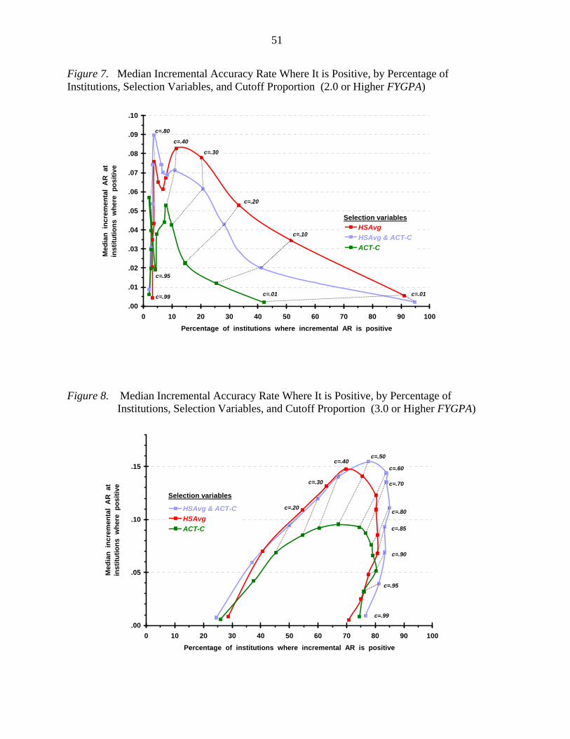
51
Figure 7. Median Incremental Accuracy Rate Where It is Positive, by Percentage of Institutions, Selection Variables, and Cutoff Proportion (2.0 or Higher FYGPA)
.00
.01
.02
.03
.04
.05
.06
.07
.08
.09
.10
0 10 20 30 40 50 60 70 80 90 100Percentage of institutions where incremental AR is positive
Med
ian
incr
emen
tal
AR
at
inst
itutio
ns w
here
pos
itive
HSAvgHSAvg & ACT-CACT-C
c=.01
c=.10
c=.20
c=.30
c=.40
c=.80
c=.99
c=.95
c=.01
Selection variables
Figure 8. Median Incremental Accuracy Rate Where It is Positive, by Percentage of
Institutions, Selection Variables, and Cutoff Proportion (3.0 or Higher FYGPA)
.00
.05
.10
.15
0 10 20 30 40 50 60 70 80 90 100Percentage of institutions where incremental AR is positive
Med
ian
incr
emen
tal
AR
at
inst
itutio
ns w
here
pos
itive
HSAvg & ACT-CHSAvgACT-C
c=.99
c=.95
c=.90
c=.50
c=.60
c=.70
c=.85
c=.80
c=.40
c=.30
c=.20
Selection variables

52
For the 3.5 success level (see Figure 9 on the following page), HSAvg has incremental
accuracy at a majority of institutions for cutoff proportions .85 and higher, and ACT-C has
incremental accuracy at a majority of institutions for cutoff proportions .90 and higher. ACT-C
is more effective, in terms of median incremental accuracy, than HSAvg at these cutoff
proportions; the median incremental accuracy for both selection variables, however, is below .05.
Interestingly, at a small proportion of institutions, HSAvg and HSAvg & ACT-C jointly have very
large incremental accuracy (about .25) near cutoff proportion .30.
According to Figure 9, HSAvg & ACT-C jointly is better than HSAvg alone for cutoff
proportions above .40. Therefore, ACT-C has incremental benefit over HSAvg alone for
increasing accuracy rate for these cutoff proportions.
At the 3.7 success level (see Figure 10 on following page), HSAvg does not have
incremental accuracy at more than 20% of institutions for any cutoff proportion. Among the
institutions where it does have incremental accuracy, the median incremental accuracy is
typically less than .05. In contrast, ACT-C and the joint HSAvg & ACT-C selection variables
have incremental accuracy at a majority of institutions at cutoff proportions .95 and higher. The
median incremental accuracy at these cutoff proportions is also less than .05, however. At cutoff
proportions .70 to .90, the joint HSAvg & ACT-C selection variable has incremental accuracy at
fewer institutions, but its median incremental accuracy is larger than .05 at these institutions.
According to Figure 10, HSAvg & ACT-C jointly is better than HSAvg alone for all cutoff
proportions. In other words, ACT-C has incremental benefit over HSAvg alone at all cutoff
proportions for the 3.7 success level.

53
Figure 9. Median Incremental Accuracy Rate Where It is Positive, by Percentage of Institutions, Selection Variables, and Cutoff Proportion (3.5 or Higher FYGPA)
.00
.05
.10
.15
.20
.25
.30
0 10 20 30 40 50 60 70 80 90 100Percentage of institutions where incremental AR is positive
Med
ian
incr
emen
tal
AR
at
inst
itutio
ns w
here
pos
itive
HSAvg & ACT-CACT-CHSAvg
c=.99
c=.95c=.90
c=.85c=.80
Selection variables
c=.70c=.60c=.50c=.40
c=.30
Figure 10. Median Incremental Accuracy Rate Where It is Positive, by Percentage of
Institutions, Selection Variables, and Cutoff Proportion (3.7 or Higher FYGPA)
.00
.01
.02
.03
.04
.05
.06
.07
.08
.09
.10
0 10 20 30 40 50 60 70 80 90 100Percentage of institutions where incremental AR is positive
Med
ian
incr
emen
tal
AR
at
inst
itutio
ns w
here
pos
itive
HSAvg & ACT-CACT-CHSAvg
c=.95
c=.99
c=.90
c=.85
c=.70
c=.80
Selection variables

54
Incremental accuracy rate of ACT-C with respect to HSAvg
As shown in Table 11, the incremental accuracy rate of ACT-C with respect to HSAvg
(Equation (13)) is similar to the incremental success rate of ACT-C with respect to HSAvg: ACT-
C has little incremental accuracy with respect to HSAvg for the 2.0 success level, but it increases
with success level. The maximum increase in accuracy rate associated with adding ACT-C to a
selection rule based on HSAvg is about .04.
TABLE 11
Median Incremental Accuracy Rate of ACT-C with Respect to HSAvg,
by First-Year GPA Success Level and Cutoff Proportion
Success level
Cutoff proportion
Approx. value of HSAvg
2.0 3.0 3.5 3.7
.01 1.7 .00 .00 .00 .00
.10 2.4 .00 .00 .00 .00
.20 2.7 .00 .00 .00 .00
.30 3.0 .00 .00 .00 .00
.40 3.2 .00 .00 .00 .00
.50 3.3 .00 .01 .02 .01
.60 3.5 .01 .02 .03 .02
.70 3.7 .00 .03 .03 .03
.80 3.8 .00 .03 .04 .04
.85 3.9 .01 .03 .04 .04
.90 3.95 .01 .03 .03 .04
.95 4.0 .00 .02 .02 .03
.99 4.0 .00 .01 .01 .01
The second column of Table 11 suggests that for the 3.0, 3.5, and 3.7 success levels,
ACT-C typically has incremental accuracy with respect to HSAvg when HSAvg is 3.3 or greater.
Score Senders vs. Enrolled Students
The selection rates and accuracy rates obtained from the enrolled students only (results
available from author) were very similar to those obtained from the combined group of non-

55
enrolled score senders and enrolled students. Because applicants are midway between score
senders and enrolled students in their mean HSAvg and ACT-C, we have some assurance that the
results for score senders also apply to applicants.
Summary and Discussion
The usefulness of selection variables depends on the goals intended by decision makers.
In college admission, one plausible goal is to maximize the success rate (SR) of enrolled students
with respect to some outcome variable (e.g., first-year GPA). Another plausible goal is to
maximize the accuracy rate (AR) of an institution’s decisions to admit or reject applicants. When
the selection variable and outcome variable have a bivariate normal distribution with correlation
coefficient ρ , the SR and AR indicators of usefulness are functions of the success level, the
cutoff proportion (proportion of applicants not admitted), and ρ . It is perhaps for this reason
that people often interpret ρ as an indicator of usefulness. The bivariate normal assumption is
not realistic in college admission, however, because HSAvg has a pronounced skew. This study
suggests that SR and AR can depart substantially from values calculated from ρ .
Both HSAvg and ACT-C predict academic success in the first year of college. As shown
in Figures 2 and 3, however, their probability-of-success curves vary with different levels of
success and with different cutoff proportions. Both variables have steeper slopes for the higher
levels of success (S30, S35, and S37) than for the minimal level of success (S20). HSAvg is a
stronger predictor than ACT-C for S20, but ACT-C is much stronger than HSAvg for predicting
S35 and S37. HSAvg does better at lower cutoff proportions, and ACT-C does better at higher
cutoff proportions.
The statistical relationship of HSAvg and ACT-C with any level of success also depends
on the joint values of both predictors (Figure 4). HSAvg is a much stronger predictor among

56
students with high ACT-C scores than among students with low ACT-C scores. Correspondingly,
ACT-C is a much stronger predictor among students with high values of HSAvg than among
students with low values of HSAvg.
There is moderate variation among institutions in all the intercept and slope coefficients
defining the conditional probability of success functions. Typically, the standard deviations of
the coefficients among institutions are about two-tenths to three-tenths of the corresponding
mean values. This variation indicates that institutions would benefit from doing their own local
predictive validity studies, rather than relying on global studies.
Institutions can use either HSAvg or ACT-C to increase their success rates beyond the
base success rate, no matter which success level they choose. HSAvg is more effective than
ACT-C for increasing success rates at low to moderate cutoff proportions, but ACT-C is more
effective at higher cutoff proportions. Using both selection variables, however, is more
beneficial for improving success rates than using either variable by itself for cutoffs above
HSAvg=3.5 or ACT-C=22.
Increasing accuracy rates, beyond that associated with the null decisions of either
admitting all applicants or denying admission to all applicants, is more difficult than increasing
success rates. The reason is that accurate classification requires both the success of admitted
applicants and the failure of non-admitted applicants. The effectiveness of both HSAvg and
ACT-C for increasing accuracy rates depends strongly on the success level:
• For the minimal 2.0 success level, neither HSAvg nor ACT-C increase accuracy rate at
a majority of institutions, except at very low cutoff proportions. A possible reason for
this result is that institutions do not admit students whose HSAvg or ACT-C score

57
suggests that they are unlikely to earn at least a 2.0 FYGPA, and that lack of success
at this level is due to other reasons.
• For the 3.0 success level (representing typical performance), HSAvg and ACT-C
individually increase accuracy rate at most institutions for a broad range of cutoff
proportions. HSAvg is effective at somewhat more institutions than ACT-C at cutoff
proportions below .85, but ACT-C is effective at somewhat more institutions than
HSAvg at higher cutoff proportions.
• For the 3.5 success level, both HSAvg and ACT-C individually increase accuracy rate
at most institutions, but only at high cutoff proportions.
• For the 3.7 success level, HSAvg does not increase accuracy rate at most institutions
for any cutoff proportion. ACT-C, however, increases accuracy at most institutions
for high cutoff proportions
For all success levels, ACT-C has incremental accuracy beyond HSAvg at most institutions for
cutoffs above HSAvg=3.3 or ACT-C=20 to 21.
These results are based on the assumption that institutions use strict cutoff proportions (c)
in making admission decisions. This assumption is rarely if ever true, but it is necessary for this
research, given the absence of quantifiable rules and data on institutions’ actual admission
policies. Institutions use other variables, in addition to high school course work, grades, and test
scores, in making admission decisions. One should therefore interpret the results of this study
with this in mind.
On the other hand, self-selection by potential applicants, based on their high school
grades and test scores, might be as important as institutions’ actual admission decisions in
determining the colleges in which students enroll (see discussion following Table 4). From this

58
perspective, high school grades and test scores contribute indirectly to attaining institutions’
goals. This study captures some of the indirect contribution through its consideration of data
from score senders. High school GPA and test scores likely also contribute, however, to the
decisions by a broader pool of students to become score senders. Although the current study
does not address the extent of this additional indirect contribution, one could presumably model
it by making assumptions about the composition of the broader pool of all graduating high
school students.
With these limitations in mind, we can conclude that the conventional wisdom based on
correlations is correct in many, but not all respects. HSAvg by itself is better than ACT-C by
itself for some, but not for all, degrees of selectivity and definitions of success. In some
situations (for example, where an institution is interested in high levels of success), ACT-C is
more useful. This study affirms the other aspect of the conventional wisdom, however: In most
scenarios, using both high school grades and test scores jointly is better than using either by
itself. In using both variables, moreover, it is important to take into account the HSAvg by ACT-
C interaction effect, as well as the main effects.
Finally, it is worthwhile to keep in mind that although increasing SR and AR in making
admission decisions is a plausible goal at many institutions, it is not their only goal. Other goals,
such as objectivity and uniformity in making admission decisions, and providing data for
counseling, placement, and institutional self-study are also important, and both high school
grades and test scores contribute in different ways to these goals.

59
References ACT (1999). Prediction research summary tables. (Available from ACT, Inc., P. O.
Box 168, Iowa City, Iowa 52243). ACT (2008a). The ACT user handbook. Iowa City, Iowa: Author. Retrieved July 27,
2009 from http://www.act.org/aap/pdf/ACT_User_Handbook.pdf. ACT (2008b). The ACT Institutional Data Questionnaire. Iowa City, Iowa: Author.
Retrieved July 27, 2009 from http://www.act.org/idq/pdf/IDQBrochure.pdf. ACT (2008c). Updated validity statistics for ACT Prediction Service. (Available from
ACT, Inc., P. O. Box 168, Iowa City, Iowa 52243). ACT (2009a). ACT Class Profile Report, 2008-2009 Freshmen. Retrieved October 5,
2009 from http://www.act.org/research/services/pdf/ClassProfileNormReport.pdf. ACT (2009b). College student retention and graduation rates from 2000 to 2009.
Retrieved November 11, 2009 from http://www.act.org/research/policymakers/reports/graduation.
Allen, J., Robbins, S., Casillas, A., & Oh, I.-S. (2008). Third-year college retention and
transfer: Effects of academic performance, motivation, and social connectedness. Research in Higher Education, 49(7), 647–664.
Bowen, W., Chingos, M., & McPherson, M. (2009). Crossing the finish line:
Completing colleges at America’s public universities. Princeton, NJ: Princeton University Press.
Breland, H., Maxey, J., Gernand, R., Cumming, T., & Trapani, C. (2002). Trends in
college admissions: A report of a survey of undergraduate admissions policies, practices, and procedures. Retrieved February 3, 2010 from the Association for Institutional Research web site: http://www.airweb.org/images/trendsreport.pdf/.
Brookhart, S. M. (1993, Summer). Teachers’ grading practices: Meaning and values.
Journal of Educational Measurement, 30(2). Camara, W. (2005). Broadening criteria of college success and the impact of cognitive
predictors. In Camara, W. & Kimmel, E. (Eds.), Choosing students: Higher education admission tools for the 21st century. Mahwah, NJ: Lawrence Erlbaum Associates.
Casillas, A., Robbins, S. B., Allen J., Kuo, Y. K., Hanson, M. A., & Schmeiser, C.
(2010). Predicting early academic failure in high school from prior academic achievement, psychosocial characteristics, and behavior. (Available from ACT, Inc., P. O. Box 168, Iowa City, Iowa).

60
Cizek, G. J., Fitzgerald, S. M., & Rachor, R. E. (1995/1996). Teachers’ assessment
practices: Preparation, isolation, and the kitchen sink. Educational Assessment, 3(2), 159–179.
Geisinger, K. (June, 2009). A college admission question: What would we do if the
ACT and SAT did not exist? NCME newsletter, 17(2). Retrieved July 23, 2009 from http://www.ncme.org/pubs/pdf/vol_17_num_2.pdf.
Kobrin, J. L., Patterson, B. F., Shaw, E. J., Mattern, K. D., & Barbuti, S. M. (2008).
Validity of the SAT for predicting first-year college grade point average. New York: College Board. Retrieved July 23, 2009 from http://professionals.collegeboard.com/data-reports-research/cb/validity-of-sat-predicting-fycgpa.
Kobrin, J. L. & Patterson, B. F. (2010, April). Exploring the variability in the validity of
SAT scores for predicting first-year college grades at different colleges and universities. Paper presented at the meeting of the American Educational Research Association, Denver, Colorado.
Laird, R. (2005). What is it we think we are trying to fix and how should we fix it? A
view from the admissions office. In Camara, W. & Kimmel, E. (Eds.), Choosing students: Higher education admission tools for the 21st century. Mahwah, NJ: Lawrence Erlbaum Associates.
Lord, F. M. & Novick, M. R. (1968). Statistical theories of mental test scores. Reading,
MA: Addison-Wesley. Morgan, R. (1989). Analyses of the predictive validity of the SAT and high school grades
from 1976 to 1985. New York: College Board. Retrieved July 23, 2009 from http://professionals.collegeboard.com/data-reports-research/cb/sat-validity-1976-1985.
Noble, J. P. & Sawyer, R. L. (2004). Is high school GPA better than admission test
scores for predicting academic success in college? College and University Journal, 79(4), 17-22.
Noble, J. P., Roberts, W. L., & Sawyer, R. L. (2006). Student achievement, behavior,
perceptions, and other factors affecting ACT scores (ACT Research Report Series 2006-1). Retrieved September 10, 2009 from http://www.act.org/research/researchers/reports/pdf/ACT_RR2006-1.pdf.
Raudenbush, S., Bryk, A., Cheong, Y. F., & Congdon, R. (2004). HLM6: Hierarchical
linear and nonlinear modeling. Lincolnwood, IL: Scientific Software International, Inc.

61
SAS Institute (2008). The NLMIXED Procedure (SAS/STAT User’s Guide). Cary, NC: SAS Institute. Retrieved May 14, 2010 from http://support.sas.com/onlinedoc/913/docmainpage.jsp
Saupe, J. L. & Curs, B. R. (2008). Driving enrollment management scores from ACT
data. IR Applications, 16(15). Sawyer, R. L. (1996). Decision theory models for validating course placement tests.
Journal of Educational Measurement, 33(3), 271-290. Sawyer, R. (2007). Indicators of usefulness of test scores. Applied Measurement in
Education, 20(3), 255-271. Snijders, T. A. B. & Bosker, R. J. (1999). Multilevel analysis. Thousand Oaks, CA:
Sage. Stiggins, R. J., Frisbie, D. A., & Griswold, P. A. (1989). Inside high school grading
practices: Building a research agenda. Educational Measurement: Issues and Practice, 8(2), 5–14.
Willingham, W. (2005). Prospects for improving grades for use in admissions. In
Camara, W. & Kimmel, E. (Eds.), Choosing students: Higher education admission tools for the 21st century. Mahwah, NJ: Lawrence Erlbaum Associates.
Woodruff, D. J. & Ziomek, R. L. (2004). High School Grade Inflation from 1991 to
2003. Iowa City, Iowa: ACT, Inc. Retrieved July 23, 2009 from http://www.act.org/research/researchers/reports/pdf/ACT_RR2004-4.pdf.

62

63
Appendix
Relationship of Conditional Probability of Success and Its Marginal Distribution with Success Rate and Accuracy Rate
Proposition 1: Let ( ) [ xPxp =Χ= Success ] be strictly increasing in x =be the probability density function for( )xf Χ . Assume that is non-zero everywhere. f Let ( ) ( ) ( ) ( )∫∫
∞∞=
kkdxxfdxxfxpkSR be the success rate for a cutoff score , and
let . Then:
k
)(SRBSR −∞=1. SR is strictly increasing in x. 2. SR(x) > BSR. 3. SR(x) > p(x).
Proof:
LetBA
dttf
dttftpxSR
x
x ==∫
∫∞
∞
)(
)()()( .
[ ].)()(
)()()(
)(Then
2
2
2
BxBpAxf
BxAfBxpxf
BBABAxRS
−=
+−=
′−′=′
,)(
)()()()( ,increasing is Since
Bxp
dttfxpdttftpApx x
=
>= ∫ ∫∞ ∞
and therefore, Thus, SR is strictly increasing in x, and . 0)( >′ xRS .)()( BSRSRxSR =−∞>
Because [ ] 0)()(2 >−
BxBpAxf for all x, for all x, and so
for all x. ∫ ∫∞ ∞
<x x
dttftpdttfxp )()()()(
)()( xpxSR >

64
Proposition 2: Given the previous assumptions, let be the
accuracy rate associated with cutoff score . Then, AR has a local maximum at if, and only if,
( ) ( )[ ] ( ) ( ) ( )∫∫∞
∞−+−=
k
kdxxfxpdxxfxpkAR 1
k 0k( ) 210 =kp .
Proof:
( ) ( )[ ] ( ) ( ) ( )kfkpkfkpkRA −−=′ 1 . ( ) ( ) ( )kfkpkf 2−=
( ) 00 =′ kRA if, and only if, ( ) ( ) ( )0002 kfkfkp =− . Since ( ) ( ) ( ) 21if,only and if,0,0 000 ==′> kpkRAkf . Note that ( ) ( ) ( ) ( ) ( ) ( )[ ]kfkpkfkpkfKRA ′+′−′=′′ 2 . Therefore ( ) ( ) ( ) ( ) ( )00000 2 kfkfkpkfKRA ′−′−′=′′ ( ) ( ) ( ) .21 since ,2 000 =′−= kpkfkp Because ( ) ( ) ( ) .0,0 and 0 000 <′′>>′ kRAkfkp
Therefore, AR has a local maximum at if, and only if, 0k ( ) 210 =kp .
Proposition 3: Let . Then max AR exceeds BSR and 1-BSR if, and only if, p crosses 1/2. ( ) ( )∫
∞
∞−= dxxfxpBSR
Proof: Suppose for some k. Proof by contradiction: ( ) BSRkAR > Suppose ( ) 21>xp for all x . Then . ( )[ ] ( ) ( ) ( )∫∫ ∞−∞−
<−kk
dxxfxpdxxfxp1
And so, ( ) ( ) ( ) ( ) ( )∫∫
∞
∞−+<
k
kdxxfxpdxxfxpkAR
=BSR [contradiction]. If ( ) , allfor 21 xxp < then . ( ) ( ) ( )[ ] ( )∫ ∫
∞ ∞−<
k kdxxfxpdxxfxp 1

65
And so, ( ) ( )[ ] ( ) ( )[ ] ( )∫ ∫∞−
∞−+−<
k
kdxxfxpdxxfxpkAR 11
( )[ ] ( )
.tion][contradicBSR
dxxfxp
1
1
−=
−= ∫∞
∞−
Therefore ( ) 210 =kp for some . 0k Since p is monotonic increasing, p must cross 21 at . 0k Now, suppose p crosses 21 . Let ( ) 210 =kp and ( ) ( ) ,21and,for ,21 0 ><< xpkxxp .for 0kx > Then ( ) ( )[ ] ( ) ( ) ( )∫∫
∞
∞−+−=
0
0 10 k
kdxxfxpdxxfxpkAR
( ) ( ) ( ) ( )
.BSR
dxxfxpdxxfxpk
k
=
+> ∫∫∞
∞− 0
0
Also, ( ) ( )[ ] ( ) ( ) ( )∫ ∫∞−
∞+−= 0
0
10
k
kdxxfxpdxxfxpkAR
( )[ ] ( ) ( )[ ] ( )
.BSR
dxxfxpdxxfxpk
k
−=
−+−> ∫∫∞
∞−
1
110
0