Embed Size (px)
Citation preview
The Usefulness of
Direct Cash Flow Statements
under IFRS
by
Alan Jonathan Duboisée de Ricquebourg
Submitted in accordance with the requirements for the degree of
Doctor of Philosophy
The University of Leeds
Leeds University Business School
Accounting and Finance Division
Centre for Advanced Studies in Finance
May 2013

Intellectual Property Statement i
Intellectual Property Statement
The candidate confirms that the work submitted is his own and that appropriate credit
has been given were reference has been made to the work of others.
This copy has been supplied on the understanding that it is copyright material and that
no quotation from the thesis may be published without proper acknowledgement.
© 2013 The University of Leeds and Alan Duboisée de Ricquebourg

Dedication of this Thesis ii
Dedication of this Thesis
To my beautiful wife Rachel, thank you for your love, support, encouragement, and
prayers throughout my doctoral studies.

Acknowledgements iii
Acknowledgments
All the glory and praise for this thesis belongs to my Lord and saviour Jesus Christ for
providing me with the focus, discipline, and support to complete this project.
It gives me great pleasure in acknowledging my primary supervisor, Dr Iain Clacher,
for his guidance, support, encouragement, and many thought provoking discussions
throughout my doctoral studies. Further, I am grateful to my second supervisor,
Professor Allan Hodgson, for his valuable input and guidance in my thesis. In addition,
I would like to thank Professor David Hillier for encouraging me to pursue this doctoral
study, and for his support and guidance in the early stages of my thesis. I am obliged to
many of my colleagues, both at the Centre for Advanced Studies in Finance, and within
the Accounting and Finance division of Leeds University Business School for the
numerous thought provoking conversations and encouragement over the past years.
Special mention goes to Michelle Dickson for her tireless enthusiasm, support, and
encouragement.
I am eternally grateful for my friends and family, especially my parents, Kevin and
Jocelyn, and my father and mother in law, Mark and Helga, who have constantly prayed
for and encouraged me over the years. My deepest gratitude, I owe to my beautiful wife
Rachel, to whom I have dedicated this thesis, for her love, patience, encouragement,
prayer, and support throughout my doctoral studies.
Finally, I am truly indebted and thankful to the Centre for Advanced Studies in
Finance (CASIF) for their financial support, without which it would have been
impossible to complete this thesis.
Abstract iv
Abstract
The International Accounting Standards Board (IASB) and Financial Accounting
Standards Board (FASB) have recently proposed to mandate the use of direct cash flow
statements as part of their project to harmonise accounting standards. Despite the
magnitude of the proposed change to cash flow reporting, to date, the IASB and FASB
have provided no empirical evidence under International Financial Reporting Standards
(IFRS) to support their assertion that direct cash flow statements provide financial
statement users with useful information. Given the growing evidence that adopting
IFRS significantly changes the quality of financial reporting information, the usefulness
of direct cash flow statements may have also changed. This thesis, therefore, examines
the usefulness of reporting direct cash flow statements under IFRS in Australia.
Australia is specifically examined because it was one of the few countries where all
firms were mandated to report direct cash flow statements, and which prohibited the
early adoption of IFRS.
The findings of this research show that, relative to Australian Generally Accepted
Accounting Principles (AGAAP), direct cash flow statements are more value relevant
after the adoption of IFRS. Moreover, the results demonstrate that direct cash flow
statements provide financial analysts with useful information for their cash flow
forecasts, and this information is more useful under IFRS compared to AGAAP. Finally,
this thesis provides evidence that, while financial analysts use information from direct
cash flow statements when issuing stock recommendations, buy-and-hold investors are

Abstract v
better off identifying mispriced stocks by using analysts’ cash flow forecasts in
discounted cash flow valuation models.
In sum, these results provide strong support for the current IASB/FASB proposal to
mandate the use of direct cash flow statements and are consistent with IFRS improving
the information set of investors.
Table of Contents vi
Table of Contents
Acknowledgments ......................................................................................................... iii
Abstract...........................................................................................................................iv
Table of Contents ...........................................................................................................vi
List of Tables ...................................................................................................................x
List of Figures.............................................................................................................. xiii
List of Abbreviations ....................................................................................................xv
1 Introduction..............................................................................................................1
1.1 Introduction ........................................................................................................1
1.2 Contributions of the Thesis ................................................................................4
1.2.1 The Value Relevance of Direct Cash Flows under IFRS............................5
1.2.2 Direct Cash Flow Statements and Analyst Cash Flow Forecast Accuracy
under IFRS.................................................................................................................5
1.2.3 Are Analysts’ Cash Flow Forecasts and Direct Cash Flow Statements
Essential Inputs to Generate Stock Recommendations?............................................6
1.3 Structure of the Thesis........................................................................................7
2 The Historical Development of Cash Flow Reporting........................................10
2.1 Introduction ......................................................................................................10
2.1.1 Recording Cash Flows: The Oldest Form of Accounting.........................10
2.1.2 From The Balance Sheet to the Income Statement ...................................10
2.2 The American Influence on Cash Flow Reporting...........................................12
2.2.1 The Development of the Funds Flow Statement in America....................13
2.2.2 The Evolution to the Cash Flow Statement in America............................17
2.3 The Development of Cash flow reporting in the U.K. .....................................20
2.3.1 The Development of Funds Flow Reporting in the U.K...........................20
2.3.2 The Issue of FRS 1 Cash Flow Statements ...............................................23
Table of Contents vii
2.3.3 The U.K. Transition to IFRS and its Effect on Cash Flow Reporting ......27
2.4 The Development of Cash flow Reporting in Australia...................................28
2.4.1 The Development of Funds Flow Reporting in Australia.........................28
2.4.2 The Development of Cash Flow Reporting in Australia...........................31
2.4.3 The Australian Transition to IFRS............................................................32
2.5 The Development of Cash flow Reporting by the IASC/IASB .......................34
2.5.1 The Development of Funds Flow Reporting by the IASC........................34
2.5.2 The Issue of IAS 7 “Cash Flow Statements” ............................................34
2.6 The FASB and IASB Convergence Project .....................................................37
2.7 Summary and Conclusion ................................................................................39
3 Literature Review ..................................................................................................42
3.1 Introduction ......................................................................................................42
3.2 Empirically Examining the Usefulness of Operating Cash Flows ...................45
3.2.1 Using Cash Flow Data to Forecast Future Cash Flows and Earnings.......45
3.2.2 Using Cash Flow Data to Explain Capital Market Effects .......................53
3.3 The Impact of Adopting IFRS..........................................................................58
3.3.1 Economic Effects from Mandatory IFRS Reporting ................................61
3.3.2 Capital Market Effects from Mandatory IFRS Reporting.........................62
3.3.3 Impact on Analyst Forecast Errors from Mandatory IFRS Reporting......63
3.4 Summary and Conclusion ................................................................................64
4 Sample Selection and Descriptive Statistics ........................................................66
4.1 Sample Selection ..............................................................................................66
4.2 Descriptive Statistics ........................................................................................70
5 The Value Relevance of Direct Cash Flows under IFRS ...................................80
5.1 Introduction ......................................................................................................80
5.2 Literature Review .............................................................................................83
5.2.1 Usefulness of Reporting Direct Cash Flows .............................................83
5.2.2 Impact of Reporting Under IFRS..............................................................85
5.2.3 Adoption of IFRS by Australia .................................................................86
5.3 Hypotheses Development.................................................................................86
Table of Contents viii
5.4 Model Development and Data..........................................................................89
5.4.1 Model Construction...................................................................................89
5.4.2 Sample Construction and Descriptive Statistics .......................................93
5.5 Empirical Results ...........................................................................................101
5.5.1 Value Relevance of Earnings and Net Assets .........................................102
5.5.2 Disaggregating Earnings .........................................................................105
5.5.3 Disaggregating Cash Flows.....................................................................107
5.5.4 Robustness Tests .....................................................................................115
5.6 Conclusions ....................................................................................................116
6 Direct Cash Flow Statements and Analyst Cash Flow Forecast Accuracy
under IFRS ..................................................................................................................118
6.1 Introduction ....................................................................................................118
6.2 Background and Hypothesis Development ....................................................120
6.2.1 Direct Cash Flows and Forecasting.........................................................120
6.2.2 Analysts’ Use of Direct Cash Flow Components ...................................123
6.2.3 IFRS Adoption and Analysts’ Use of Direct Cash Flow Components ...124
6.2.4 IFRS Adoption and Analysts’ Information Environment .......................127
6.3 Research Design and Sample Selection .........................................................129
6.3.1 Analysts’ Cash Flow Forecasts and Direct Cash Flow Components......129
6.3.2 Change in Analyst Forecast Accuracy ....................................................133
6.3.3 IFRS Adoption and Analysts’ Cash Flow Forecasts Accuracy ..............133
6.3.4 Sample Selection.....................................................................................136
6.4 Results ............................................................................................................140
6.4.1 Descriptive Statistics of Variables Used in Equations (6.1) to (6.4) ......140
6.4.2 Descriptive Statistics of Variables Used in Equation (6.6).....................145
6.4.3 IFRS Adoption and Analysts’ Use of Direct Cash Flow Components ...149
6.4.4 IFRS Adoption and Accuracy of Analysts’ Cash Flow Forecasts ..........157
6.4.5 Ranking the Empirical Models................................................................160
6.5 Discussion and Conclusion ............................................................................163
7 Are Analysts’ Cash Flow Forecasts and Direct Cash Flow Statements Essential
Inputs to Generate Stock Recommendations? .........................................................165
Table of Contents ix
7.1 Introduction ....................................................................................................165
7.2 Background and Hypothesis Development ....................................................167
7.2.1 Analysts’ Choice of Valuation Model.....................................................167
7.2.2 Analysts’ Earnings Forecasts as Valuation Inputs ..................................169
7.2.3 Analysts’ Cash Flow Forecasts as Valuation Inputs...............................172
7.2.4 Analysis of Future Excess Returns and Valuation models .....................176
7.3 Research Design .............................................................................................177
7.3.1 Using Analysts’ Earnings and Long Term Growth Forecasts ................177
7.3.2 Using Analysts’ Cash Flow Forecasts and Direct Cash Flow Information ..
.................................................................................................................181
7.4 Data, Sample and Descriptive Statistics.........................................................186
7.5 Regression Results .........................................................................................205
7.5.1 Analysis of Analysts’ Recommendations on Valuation Metrics ............205
7.5.2 Analysis of Analysts’ Recommendations on Valuation Metrics with
Further Controls .....................................................................................................210
7.5.3 Analysis of Changes in Recommendations on Changes in Valuation
Metrics .................................................................................................................214
7.5.4 Analysis of Future Excess Returns and Valuation Models.....................220
7.6 Discussion and Conclusion ............................................................................231
8 Conclusion ............................................................................................................235
8.1 Background to the Thesis ...............................................................................235
8.2 Summary of Findings .....................................................................................236
8.2.1 Direct Cash Flow Statements Increase in Value Relevance under IFRS......
.................................................................................................................236
8.2.2 Direct Cash Flow Statements Provide Financial Analysts Useful
Information for Forecasting Cash Flows ...............................................................237
8.2.3 Direct Cash Flow Statements Provide Financial Analysts and Buy-and-
Hold Investors Useful Information to Identify Mispriced Securities ....................237
8.3 Policy Implications and Direction for Further Research................................238
Bibliography ................................................................................................................240
List of Tables x
List of Tables
Table 2-1 Illustrative example of a funds flow statement...............................................13
Table 2-2 Summary of the development of cash flow reporting in the U.S. ..................14
Table 2-3 Illustrative examples of the indirect and direct method of disclosure ............19
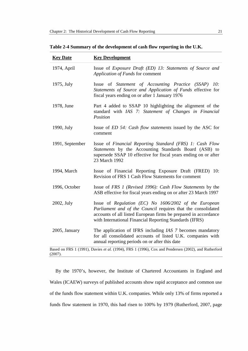
Table 2-4 Summary of the development of cash flow reporting in the U.K...................21
Table 2-5 Summary of the development of cash flow reporting in Australia.................29
Table 2-6 Summary of the development of cash flow reporting by the IASC/IASB .....35
Table 4-1 Sample selection and distribution...................................................................68
Table 5-1 Sample selection and distribution...................................................................96
Table 5-2 Descriptive statistics .......................................................................................99
Table 5-3 Comparing the value relevance of aggregate earnings and net assets before
and after the adoption of IFRS......................................................................................103
Table 5-4 Comparing the value relevance of aggregate earnings, net assets and
intangible assets before and after the adoption of IFRS ...............................................104
Table 5-5 Comparing the value relevance of operating cash flows, accruals, net assets
and intangible assets before and after the adoption of IFRS.........................................106
Table 5-6 Comparing the value relevance of core and non-core operating direct cash
flows, accruals, net assets and intangible assets before and after the adoption of IFRS
.......................................................................................................................................109
Table 5-7 Annual comparison of the value relevance of core operating direct cash flows,
accruals, net assets and intangible assets before and after the adoption of IFRS .........112
Table 5-8 Comparing the value relevance of direct operating cash flow components,
accruals, net assets and intangible assets before and after the adoption of IFRS .........114
Table 6-1 Sample selection and distribution.................................................................138
List of Tables xi
Table 6-2 Descriptive statistics of variables used in the regression analysis examining
analysts’ use of direct cash flow components when forecasting cash flows.................141
Table 6-3 Descriptive statistics of variables used in the regression analysis examining
the effect of mandatory IFRS adoption on analysts cash flow forecast errors..............146
Table 6-4 Comparing analysts’ use of operating cash flows and accruals when
forecasting future cash flows before and after the adoption of IFRS ...........................150
Table 6-5 Comparing analysts’ use of ‘core’ operating cash flows and accruals when
forecasting future cash flows before and after the adoption of IFRS ...........................152
Table 6-6 Comparing analysts’ use of direct operating cash flows, ‘non-core’ operating
cash flows and accruals when forecasting future cash flows before and after the
adoption of IFRS...........................................................................................................154
Table 6-7 Comparing analysts’ use of direct operating cash flow components and
accruals when forecasting future cash flows before and after the adoption of IFRS....156
Table 6-8 Effect of mandatory IFRS adoption on analysts’ cash flow forecast errors .158
Table 6-9 Comparing analysts’ use of operating cash flow components and accruals by
comparing the average ranks of forecast errors generated by each empirical model ...161
Table 7-1 Timeline for estimating Equation (7.1a).......................................................178
Table 7-2 Timeline for estimating Equation (7.5a).......................................................182
Table 7-3 Sample selection and distribution.................................................................189
Table 7-4 Pooled descriptive statistics.........................................................................194
Table 7-5 Descriptive statistics across recommendation quintile portfolios ................202
Table 7-6 Correlation matrix of key variables ..............................................................203
Table 7-7 Regression results of consensus recommendation and earnings variables ...207
Table 7-8 Regression results of consensus recommendation and cash flow variables .208
Table 7-9 Regression results of consensus recommendations and earnings variables with
further controls ..............................................................................................................212
List of Tables xii
Table 7-10 Regression results of consensus recommendations and cash flow variables
with further controls ......................................................................................................215
Table 7-11 Regression results of consensus recommendations changes and changes in
earnings variables and long-term growth......................................................................218
Table 7-12 Regression results of consensus recommendations changes and changes in
cash flow variables........................................................................................................219
Table 7-13 Regression results of one-year-ahead market adjusted returns on consensus
recommendations, earnings variables, and long term growth.......................................224
Table 7-14 Regression results of one-year-ahead quartile size adjusted returns on
consensus recommendations, earnings variables, and long term growth......................225
Table 7-15 Regression results of one-year-ahead market adjusted returns on cash flow
variables ........................................................................................................................228
Table 7-16 Regression results of one-year-ahead quartile size adjusted returns on cash
flow variables ................................................................................................................229
Table 7-17 Vuong test results comparing the power of earnings versus cash flow based
valuation models when explaining one-year-ahead excess returns...............................231
List of Figures xiii
List of Figures
Figure 4-1 Comparison of total market capitalisation.....................................................69
Figure 4-2 Comparison of total market capitalisation for industrial and extractive firms
.........................................................................................................................................70
Figure 4-3 Comparison between average market capitalisation and accounting variables
for industrial firms...........................................................................................................71
Figure 4-4 Comparison between average market capitalisation and accounting variables
for extractive firms..........................................................................................................72
Figure 4-5 Comparison between average operating, investing, and financing cash flows
for industrial firms...........................................................................................................74
Figure 4-6 Comparison between average operating, investing, and financing cash flows
for extractive firms..........................................................................................................75
Figure 4-7 Comparison between average earnings, accruals, and operating cash flows
for industrial firms...........................................................................................................76
Figure 4-8 Comparison between average earnings, accruals, and operating cash flows
for extractive firms..........................................................................................................77
Figure 4-9 Comparison between average cash flow variables for industrial firms.........78
Figure 4-10 Comparison between average cash flow variables for extractive firms......79
Figure 7-1 Distribution of analysts’ consensus stock recommendations ......................192
Figure 7-2 Distribution of the change in analysts’ consensus stock recommendations193
Figure 7-3 Distribution of the residual income valuation metric with fade rate
assumption ....................................................................................................................197
Figure 7-4 Distribution of the residual income valuation metric with perpetuity
assumption ....................................................................................................................198

List of Figures xiv
Figure 7-5 Distribution of the discount cash flow valuation metric with fade rate
assumption ....................................................................................................................199
Figure 7-6 Distribution of the discount cash flow valuation metric with perpetuity
assumption ....................................................................................................................200
Figure 7-7 Distribution of cumulative annual market adjusted stock returns (CAR)...221
Figure 7-8 Distribution of cumulative annual size adjusted stock returns (SAR) ........222

List of Abbreviations xv
List of Abbreviations
AARF Australian Accounting Research Foundation
AASB Australian Accounting Standards Board
AGAAP Australian Generally Accepted Accounting Principles
AICPA American Institute of Certified Public Accountants
APB Accounting Principles Board
ASSC Accounting Standards Steering Committee
ASX Australian Stock Exchange
CFA Chartered Financial Analysts
CSHPS Cash payments to suppliers and employees
CSHRC Cash receipts from customers
E.U. European Union
ED Exposure Draft
FASB Financial Accounting Standards Board
FRED Financial Reporting Exposure Draft
FRC Financial Reporting Council
FRS Financial Reporting Standards
GAAP Generally Accepted Accounting Principles
I/B/E/S Thomson Reuters Institutional Brokers' Estimate System
IAS International Accounting Standards
IASB International Accounting Standards Board
IASC International Accounting Standards Committee
ICAA Institute of Chartered Accountants in Australia
ICAEW Institute of Chartered Accountants in England and Wales
IFRS International Financial Reporting Standards
OCF Operating cash flows
SCFP Statement of Changes in Financial Position
SEC Securities Exchange Commission

List of Abbreviations xvi
SFAC Statement of Financial Accounting Concepts
SFAS Statement of Financial Accounting Standards
SSAF Statement of Source and Application of Funds
U.K. United Kingdom
U.S. United States of America
Chapter 1: Introduction 1
1Introduction
1.1 Introduction
The International Accounting Standards Board (IASB) and Financial Accounting
Standards Board (FASB) have proposed, as part of their joint project to harmonise
accounting standards, that all cash flow statements be prepared according to the direct
method.1 Historically, however, while actively promoting the direct method, the IASB
and FASB have provided preparers with a choice of either the direct or the indirect
method of cash flow statement presentation (FASB, 1987; IASB, 2010). Moreover,
when presented with this choice, less than 4% of firms in the United States of America
(U.S.), United Kingdom (U.K.), and Canada, adopted the direct method, resulting in the
overwhelming majority of firms disclosing operating cash flows using the indirect
approach (Wallace et al., 1997; Krishnan and Largay III, 2000). Only three countries,
Australia, New Zealand, and China, have ever mandated the disclosure of operating
cash flows using the direct method (Wallace et al., 1997; Clinch et al., 2002).
Unsurprisingly, therefore, the joint proposal by the IASB and FASB, to mandate the use
of direct cash flow statements, has led to widespread debate and comment on the
usefulness of this method.
A recent survey conducted by the Chartered Financial Analysts Institute (CFA
Institute), has provided the IASB and FASB with some of their strongest evidence in
support of their current proposal. From the 541 respondents, 63% of financial analysts
1 See the Proposed Accounting Standards Update FASB Staff Draft of an Exposure Draft on FinancialStatement Presentation published in July 2010 (paragraph 177).
Chapter 1: Introduction 2
agreed, or strongly agreed, that, when compared to the indirect method, a direct cash
flow statement provided better information for forecasting cash flows and evaluating
earnings quality (CFA Institute, 2009). In contrast, however, comment letters from three
of the big four accounting firms, Deloitte, KMPG and EY, all stressed that further
research was needed to investigate the costs and benefits of reporting direct cash flows,
prior to mandating their adoption (FASB, 2009, comment letters 63, 114 and 99).
PriceWaterhouseCoopers were the only big four firm to support mandating the direct
method as proposed in the discussion paper (FASB, 2009, comment letter 172).
While the recent IASB and FASB proposal generated a large response via comment
letters, the mandating of direct cash flow statements has been debated for more than
three decades. Even before cash flow disclosures were standardised, academics had
already begun to express a definitive preference for the direct approach (e.g., Paton,
1963; Heath, 1978; Lee, 1981; Thomas, 1982; Ketz and Largay III, 1987). Moreover,
after cash flow disclosure requirements became common around the world, U.S. and
Australian surveys, conducted on diverse groups of accounting and finance academics
and professionals, continued to show support for the direct approach (e.g., Jones et al.,
1995; McEnroe, 1996; Smith and Freeman, 1996; Jones and Ratnatunga, 1997; Jones
and Widjaja, 1998; Goyal, 2004). Further, a small, but growing body of empirical
evidence has found that direct cash flow statements provide useful information to
predict earnings and cash flows (e.g., Krishnan and Largay III, 2000; Arthur and
Chuang, 2008; Cheng and Hollie, 2008; Orpurt and Zang, 2009; Arthur et al., 2010;
Farshadfar and Monem, 2012, 2013), and explain stock returns (e.g., Livnat and
Zarowin, 1990; Clinch et al., 2002; Orpurt and Zang, 2009).
Chapter 1: Introduction 3
Although these findings provide support for the IASB and FASB proposal, all the
recent Australian studies, however, specifically exclude observations after the
mandatory adoption of International Financial Reporting Standards (IFRS) (e.g., Arthur
et al., 2010; Farshadfar and Monem, 2012, 2013). Arthur et al. (2010) cite the
significant changes to the financial data, caused by adopting IFRS, as reason to exclude
all observations under the new standards. There is growing evidence that, in many
cases, adopting IFRS does improve the comparability and quality of the financial
information reported by firms (e.g., Daske et al., 2008; Aharony et al., 2010; Bissessur
and Hodgson, 2011; Cotter et al., 2012; Horton et al., 2012).
Prior to Australia’s adoption of IFRS, European markets were shown to have reacted
positively to a series of announcements leading up to the European Union’s (E.U.)
adoption of IFRS (Armstrong et al., 2010). Investors clearly believed that the
mandatory adoption of IFRS by the E.U. would improve the overall quality of financial
reporting information. There is evidence to suggest that this belief of improved
accounting information under IFRS was correct. Using a global sample of IFRS
adopters, Daske et al. (2008) found a general reduction in cost of capital and improved
capital market liquidity after the mandatory adoption of IFRS, particularly when those
standards were actively enforced. Although Ball (2006) raised concerns that, under
IFRS, fair value accounting would increase earnings volatility, overall, annual reports
prepared under IFRS seem to have provided users with a richer information set than was
available under local GAAP.
The view that IFRS provides users with a richer information set is borne out by a
number of recent studies both globally and in Australia, and show a significant increase
in analysts’ earnings forecast accuracy under IFRS (Bissessur and Hodgson, 2011;
Chapter 1: Introduction 4
Cotter et al., 2012; Horton et al., 2012). These findings help support the idea that
accounts prepared under IFRS conventions present users with useful information to help
evaluate an entity’s future cash generating potential, a key goal of the IASB (IASB,
1989, paragraphs 15-18). Given the evidence that IFRS has improved the quality of
financial reporting information, it is important to examine whether the importance of
direct cash flow information changes in an IFRS environment, as it is an established
source of information, which could be complemented by the improved information set
provided by IFRS.
1.2 Contributions of the Thesis
To date, no research has examined whether direct cash flow statements provide useful
information within an IFRS reporting framework. While the IASB and FASB are yet to
make a decision on the mandatory use of direct cash flow statements, if it is decided
that only direct cash flow statements are to be allowed, such a decision would affect
cash flow reporting across most of the world. Given the significant changes made to
financial reporting with the introduction of IFRS, before a decision is made to mandate
direct cash flow statements, the IASB and FASB should understand whether direct cash
flow statements are useful in an IFRS reporting framework. The objective of this thesis
is, therefore, to understand whether or not direct cash flow statements are useful sources
of information in an IFRS setting. In doing so, this thesis provides the first evidence as
to whether the proposed mandating of direct cash flow statements would further
improve the informational environment under IFRS.
Australia prohibited the early adoption of IFRS, and mandated the use of direct cash
flow statements before and after the introduction of IFRS. Moreover, Australia is a high
Chapter 1: Introduction 5
enforcement regime and has both liquid and developed markets as well as sophisticated
users of financial accounts. Australia is, therefore, an ideal setting to investigate how
IFRS adoption may have changed the usefulness of information from direct cash flow
statements. Accordingly, by using Australian data, Chapters 5 to 7 of this thesis,
provide unique evidence regarding the usefulness of direct cash flow statements under
IFRS.
1.2.1 The Value Relevance of Direct Cash Flows under IFRS
Chapter 5 examines whether there has been a change in the value relevance of operating
cash flows and direct cash flow components since the adoption of International
Financial Reporting Standards in Australia.
Using an Ohlson (1995) model, the findings show that direct cash flows are value
relevant across all industries. Moreover, there is a significant increase in the value
relevance of operating cash flows and direct cash flow components under IFRS for
industrial firms. Overall, the findings support the proposition that direct cash flow
statements are useful to investors, providing a reliable source of price relevant
information under IFRS.
1.2.2 Direct Cash Flow Statements and Analyst Cash Flow Forecast Accuracy
under IFRS
Chapter 6 examines whether information from direct cash flow statements are used by
financial analysts in predicting future cash flows. In addition, this chapter tests whether
there has been a change in the usefulness of cash flow statements for predicting future
cash flows after the move from Australian GAAP to IFRS. Motivating this chapter is
Chapter 1: Introduction 6
the CFA survey feedback that analysts’ believe direct cash flow statements provide
useful information for forecasting future cash flows (CFA Institute, 2009).
The findings show that (i) direct cash flow components are a strong predictor of
analysts’ cash flow forecasts and (ii) this relationship has strengthened since the
adoption of IFRS. Moreover, the results show a decrease in analysts’ cash flow forecast
errors in the post-adoption period, which is partly due to analysts’ increased use of
direct cash flow components under IFRS.
1.2.3 Are Analysts’ Cash Flow Forecasts and Direct Cash Flow Statements
Essential Inputs to Generate Stock Recommendations?
Chapter 7 is the final empirical chapter, which examines whether financial analysts’ use
their cash flow forecasts when issuing stock recommendations in Australia. In addition,
the chapter tests whether information from direct cash flow statements are used by
financial analysts when identifying mispriced securities.
Prior studies demonstrate that analysts’ stock recommendations relate positively to
valuation heuristics based on their earnings forecasts, but negatively to future excess
stock returns and residual income valuations. While these findings validate the use of
analysts’ earnings forecasts as valuation inputs to identify mispriced securities, the
extant literature has left unanswered whether analysts’ cash flow forecasts are used in a
similar manner. A growing body of research has demonstrated the value relevance of
analysts’ cash flow forecasts, and recent large-scale survey results show most analysts’
believe direct cash flow statements provide useful information for forecasting future
cash flows.
Chapter 1: Introduction 7
The findings in this chapter show that analysts do use their cash flow forecasts and
historical direct cash flow information when setting stock recommendations. However,
analyst stock recommendations relate negatively to future excess stock returns and
discounted cash flow models. Overall, the results are consistent with the earnings based
studies, and demonstrate that buy-and-hold investors are best off using analysts’
forecasts in multi-period valuation models to identify mispriced securities. Moreover,
comparing the profitability of multi-period earnings vs. multi-period cash flow
valuation techniques, buy-and-hold investors are significantly better off using analyst
cash flow forecasts in discounted cash flow models for identifying mispriced securities.
1.3 Structure of the Thesis
This thesis is organised as follows:
Chapter 2 provides a historical overview of the development of cash flow reporting
in the U.S., U.K., Australia, and by the IASB. Moreover, this chapter shows, when
developing cash flow reporting standards over the past three decades, the centrality
of the debate concerning the disclosure of operating cash flows for all accounting
regulators regardless of jurisdiction. This chapter ends with an overview of the
recent proposal by the IASB and FASB, as presented in their discussion paper,
recommending the mandatory use of direct cash flow statements.
Chapter 3 reviews the extant literature examining the usefulness of direct cash flow
statements. Empirical results suggest that information from direct cash flow
statements do provide incremental explanatory power and accuracy to cash flow
prediction models in addition to explaining capital market returns. However, to date,
all empirical studies have focussed on investigating the usefulness of direct cash
Chapter 1: Introduction 8
flow statements under domestic accounting standards in either the U.S. or Australia.
No research has investigated the usefulness of direct cash flows when reported
under IFRS. Chapter 3, therefore, also provides an overview of the key studies
examining the impact of adopting IFRS around the world, showing that most studies
have found a significant improvement in financial accounting quality under IFRS.
Chapter 4 presents the sample selection criteria and high-level descriptive statistics
of the sample used in this study. In doing so, this chapter illustrates the
representative nature of the sample, and the relationship between key accounting
variables over the period. More detailed descriptive statistics and sampling and
selection criteria are presented and discussed in Chapters 5 to 7.
Chapter 5 is the first empirical chapter, which examines the value relevance of
direct cash flow statements under IFRS, and the change in value relevance of direct
cash flow statements since Australia adopted IFRS.
Chapter 6 empirically examines whether financial analysts use information from
direct cash flow statements when forecasting cash flows under Australian GAAP
and IFRS. Further, this chapter examines whether analysts find information from
direct cash flow statements more useful for forecasting cash flows under IFRS,
when compared to Australian GAAP.
Chapter 7 is the final empirical chapter, which examines whether financial analysts
use their cash flow forecasts and information from direct cash flow statements as
inputs in the process of arriving at their final output, the stock recommendation.
Further, this chapter examines whether buy-and-hold investors are better able to
identify mispriced securities by following the analysts’ recommendation or by using
analysts’ cash flow forecasts in discounted cash flow valuation models.

Chapter 1: Introduction 9
Chapter 8 provides a summary and conclusion of the thesis, an overview of the
policy implications, and direction for further research.
Chapter 2: The Historical Development of Cash Flow Reporting 10
2The Historical Development of Cash FlowReporting
2.1 Introduction
2.1.1 Recording Cash Flows: The Oldest Form of Accounting
Cash flow accounting is one of the oldest forms of record keeping dating back to the
middle ages, during which time, all recorded business deals related to actual cash
receipts or payments with no regard given to the specific timing of these transactions
(Edwards, 1996, page 32). Subsequently, double entry bookkeeping and accrual
accounting developed, precipitating a radical change to accounting, to match the costs
of resources used with the associated revenues generated by those same resources.
Matching cost and revenue streams allowed firms to calculate a profit or loss for the
reporting period, which was useful in ensuring the accuracy and completeness of the
accounting records presented to the owner (Edwards, 1996, page 33) .
2.1.2 From The Balance Sheet to the Income Statement
Soon after the creation of accrual accounting, the balance sheet grew in prominence as a
focal point within financial reporting, and remained so until the late 17th century.
Edwards (1996, page 34) report that business owners were primarily concerned with the
financial position of the firm and, therefore, placed far less importance on the profit and
loss account, which was mainly used to balance the financial records. Moreover, the
balance sheet provided owners with useful information to monitor management in the
Chapter 2: The Historical Development of Cash Flow Reporting 11
fulfilment of their role as stewards of the business. However, by the early 18th century
and rise of the industrial revolution, the focus had shifted from the balance sheet and
onto the income statement (Brown, 1971, page 9).
Between 1920 and 1940, the income statement became increasingly more important
to investors (Brown, 1971, page 57). The shift away from the balance sheet as the
principal vehicle for reporting the financial position of a firm was a direct consequence
of the rise of the modern corporation which had led to growing separation between
managers and their owners (Brown, 1971, page 48). Moreover, the increased use of the
stock market to raise external capital further shifted the focus of financial reporting off
debt holders and towards equity holders. Firms, therefore, began to enhance their
disclosures surrounding profitability, rather than focussing entirely on their ability to
repay debts as they fell due. As equity holders started using this information, the income
statement grew further in importance as a means of evaluating both managements’
performance and the future prospects of dividend and capital growth.
Although the need for information by equity holders was a major catalyst
surrounding the emergence of the income statement, two other important factors
reinforced this shift away from the balance sheet. First, external pressure for accurate
profit/loss figures came from governments demanding accurate information for the
collection of corporate income taxation. Second, rapidly rising prices in the early 20th
century resulted in the need for information to evaluate the effect of inflation on the
profitability and going concern of the businesses (Brown, 1971, page 57). Income
statements, accordingly, provided financial statement users with a good basis to
measure the effects of changing prices on the business operations.
Chapter 2: The Historical Development of Cash Flow Reporting 12
Investors, creditors, and analysts demands for more detailed financial information
soon surpassed the level of information reported by the income statement and balance
sheet alone. Firms, therefore, started voluntarily supplementing the income statement
and balance sheet with a funds flow statement.2 However, the 1987 global stock market
crash, problems with the funds flow statement, and series of corporate failures, resulted
in global reforms to cash flow reporting from the late 1980’s to early 1990’s (Thomas,
1982). Standard setters responded to the growing demand for cash flow information and
mandated the disclosure of a “cash” flow statement in the financial accounts. A key
difference between the “funds” and “cash” flow statements was that while, previously,
the “funds” flow statement was a reconciliation of the changes in working capital, the
“cash” flow statement now focussed on reconciling changes in cash and cash
equivalents.
2.2 The American Influence on Cash Flow Reporting
Initial widespread global adoption and disclosure regulation of the funds flow statement,
and subsequent cash flow statement, was pioneered and heavily influenced by standard
setting bodies within the United States of America (U.S.), with other countries
following their lead (Donleavy, 1994).3 With this in mind, the historical development of
cash flow reporting elsewhere in the world, such as in the United Kingdom (U.K.),
Australia and by the International Accounting Standards Board (IASB), makes sense
only when placed within the context of the development of cash flow reporting in the
U.S.
2 See Table 2-1 for an Illustrative example of a funds flow statement.3 See Table 2-2 for an overview of the historical development of cash flow reporting in the U.S.
Chapter 2: The Historical Development of Cash Flow Reporting 13
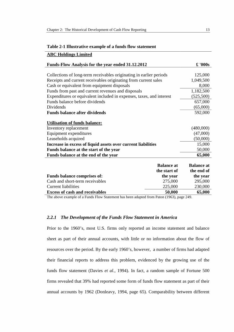
Table 2-1 Illustrative example of a funds flow statement
ABC Holdings Limited
Funds-Flow Analysis for the year ended 31.12.2012 £ '000s
Collections of long-term receivables originating in earlier periods 125,000Receipts and current receivables originating from current sales 1,049,500Cash or equivalent from equipment disposals 8,000Funds from past and current revenues and disposals 1,182,500Expenditures or equivalent included in expenses, taxes, and interest (525,500)Funds balance before dividends 657,000Dividends (65,000)Funds balance after dividends 592,000
Utilisation of funds balance:Inventory replacement (480,000)Equipment expenditures (47,000)Leaseholds acquired (50,000)Increase in excess of liquid assets over current liabilities 15,000Funds balance at the start of the year 50,000Funds balance at the end of the year 65,000
Funds balance comprises of:
Balance atthe start of
the year
Balance atthe end of
the yearCash and short-term receivables 275,000 295,000Current liabilities 225,000 230,000Excess of cash and receivables 50,000 65,000The above example of a Funds Flow Statement has been adapted from Paton (1963), page 249.
2.2.1 The Development of the Funds Flow Statement in America
Prior to the 1960’s, most U.S. firms only reported an income statement and balance
sheet as part of their annual accounts, with little or no information about the flow of
resources over the period. By the early 1960’s, however, a number of firms had adapted
their financial reports to address this problem, evidenced by the growing use of the
funds flow statement (Davies et al., 1994). In fact, a random sample of Fortune 500
firms revealed that 39% had reported some form of funds flow statement as part of their
annual accounts by 1962 (Donleavy, 1994, page 65). Comparability between different
Chapter 2: The Historical Development of Cash Flow Reporting 14
firms funds flow statements quickly became a problem, however, due to a lack of
adequate regulation. Accordingly, in 1961 the American Institute of Certified Public
Accountants (AICPA) intervened by initiating the launch of Accounting Research Study
No. 2 - “Cash Flow” Analysis and The Funds Statement, in an effort to standardise
their disclosure (Savoie, 1965).
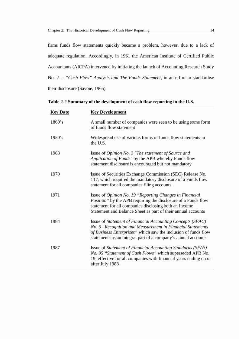
Table 2-2 Summary of the development of cash flow reporting in the U.S.
Key Date Key Development
1860’s A small number of companies were seen to be using some formof funds flow statement
1950’s Widespread use of various forms of funds flow statements inthe U.S.
1963 Issue of Opinion No. 3 "The statement of Source andApplication of Funds" by the APB whereby Funds flowstatement disclosure is encouraged but not mandatory
1970 Issue of Securities Exchange Commission (SEC) Release No.117, which required the mandatory disclosure of a Funds flowstatement for all companies filing accounts.
1971 Issue of Opinion No. 19 “Reporting Changes in FinancialPosition” by the APB requiring the disclosure of a Funds flowstatement for all companies disclosing both an IncomeStatement and Balance Sheet as part of their annual accounts
1984 Issue of Statement of Financial Accounting Concepts (SFAC)No. 5 “Recognition and Measurement in Financial Statementsof Business Enterprises” which saw the inclusion of funds flowstatements as an integral part of a company’s annual accounts.
1987 Issue of Statement of Financial Accounting Standards (SFAS)No. 95 “Statement of Cash Flows” which superseded APB No.19, effective for all companies with financial years ending on orafter July 1988
Chapter 2: The Historical Development of Cash Flow Reporting 15
Responding to the findings of AICPA in October 1963 the Accounting Principles
Board (APB) issued their Opinion No. 3 “The Statement of Source and Application of
Funds”, which recommended, but did not mandate, the use of a “Statement of Source
and Application of Funds” (SSAF) as a supplementary part of a company’s annual
accounts (CFA Institute, 1964, page 14). Industry support for this standard was
overwhelming, and by 1967 a random sample of Fortune 500 firms revealed 89% had
voluntarily disclosed the SSAF (Donleavy, 1994, page 65) .
Growing acceptance and use of the SSAF, accordingly, motivated the U.S. Securities
and Exchange Commission (SEC) to issue their Release No. 117 in 1970, mandating the
inclusion of a SSAF for all companies required to file their annual accounts with them
(Savoie, 1965). By March 1971, not long after the SEC release, the APB superseded
their prior Opinion No. 3, and issued Opinion No. 19 – “Reporting Changes in
Financial Position” mandating the disclosure of a renamed “Statement of Changes in
Financial Position” (SCFP) for all companies disclosing an income statement and
balance sheet as a part of their annual accounts.
Subsequently, however, a number of papers were highly critical of the mandated
SCFP as required by APB No. 19. Comments stated that the funds flow statement was
confusing, misleading and ambiguous (Holmes, 1976; Taylor, 1979; Han, 1981; Smith,
1985; cited in Donleavy, 1994, page 68). Moreover, the loose definition of “funds” by
the standard, which could be either “working capital” or “cash”, was heavily criticised
(Spiller and Virgil, 1974; Swanson and Vangermeersch, 1981; Ketz and Kochanek,
1982; Clark, 1983; Bryant, 1984; cited in Donleavy, 1994, page 68).
An empirical study by Spiller and Virgil (1974) continued to find significant
differences between the funds flow statements disclosed by their sample of 143 public
Chapter 2: The Historical Development of Cash Flow Reporting 16
firms, mainly due to different interpretations of the requirements of APB No. 19. They
concluded that the standard had significant weaknesses in clearly defining one overall
purpose of the SCFP. The current purpose of APB No. 19 appeared mixed between
reporting flows into and out of a “body of funds” and accounting for the movements in
balance sheet accounts. Even the Financial Accounting Standards Board (FASB)
acknowledged:
“The lack of clear objectives for the statement of changes in financial position…”
(FASB, 1987, paragraph 2)
A subsequent critical review of disclosed funds flow statements performed by Drtina
and Largay III (1985) compared the SCFP’s from three listed entities. Their findings
further highlighted the significant caveats contained within APB No. 19 whilst at the
same time motivating the use of the direct method to report operating cash flows. This
method reported gross operating cash flows directly on the face of the cash flow
statement, as opposed to the indirect approach, which calculated the net operating cash
flow by adjusting the net profit for accruals and non-cash amounts. Drtina and Largay
III (1985) demonstrated the direct method more accurately and clearly portrayed the
firms operating cash flows, especially since APB No. 19 inadequately defined
operations.
While most papers were highly critical of APB No. 19, some did comment positively
that the SCFP provided useful information which could improve the accuracy of
forecasting cash flows and business failures (Siegel and Simon, 1981; Byrd and Byrd,
1986; Coker, 1986; Gentry et al., 1987; cited in Donleavy, 1994, page 67).
Chapter 2: The Historical Development of Cash Flow Reporting 17
2.2.2 The Evolution to the Cash Flow Statement in America
Responding to the growing criticisms levelled against APB No. 19, the FASB issued
Statement of Financial Accounting Standards (SFAS) No. 95 “Statement of Cash Flows”
which superseded APB No. 19, effective for all companies with financial years ending
after July 1988 (FASB, 1987). The U.S. was one of the first countries to introduce a
standard on cash flow disclosure. 4 Although the standard was issued primarily to
eliminate the ambiguities of APB No. 19, it also developed as a result of FASB
completing their conceptual framework and issuing the Statement of Financial
Accounting Concepts (SFAC) No. 5 “Recognition and Measurement in Financial
Statements of Business Enterprises”. SFAC No. 5 saw the inclusion of cash flow
statements as an integral part of a company’s annual accounts (Donleavy, 1994).
SFAS No. 95 clarified the definition of cash flows and purpose of the standard,
requiring the classification of cash receipts and payments according to whether they
arose from operating, investing or financing activities. The purpose of the standard was
to provide relevant information about cash receipts and payments during the period in
order for users to be able to:
“…assess the enterprises ability to generate positive future net cash flows...meet
its obligations...assess the reasons for the differences between net income and
associated cash receipts and payments...and assess the effects on an enterprise’s
4 Although the U.S. was the first country to pioneer the development of the funds flow statement, theywere actually the second country to replace their funds flow statement with a cash flow statement,preceded by Canada. In 1985 the Canadian Institute of Chartered Accountants (CICA) issued TheStandard no. 1540 “Statement of Changes in Financial position” requiring the disclosure of a cash flowstatement as part of a complete set of accounts for all businesses (Donleavy, 1992). Comparisons of theseand other major cash flow reporting standards issued around the world has been summarised by Wallaceet al. (1997).
Chapter 2: The Historical Development of Cash Flow Reporting 18
financial position of both its cash and non-cash investing and financing
transactions during the period.”
(FASB, 1987, paragraphs 4-6)
This definition made it clear that FASB designed SFAS No. 95 with the main
objective of providing users with information to better estimate future cash flows in
order to determine the firm’s ability to meet their future obligations. FASB further
anticipated the informational benefits from reporting actual cash receipts and payments,
in addition to a reconciliation of operating profits to cash flows, which could be useful
in assessing the persistence of historical earnings. This information could help measure
the impact of accrual accounting on the underlying profitability and future cash
generating capacity of the enterprise.
Standard setters, therefore, explicitly declared their preference for the direct
disclosure of cash flows arising from operating activities through the presentation of
gross cash receipts and payments on the face of the cash flow statement. This approach
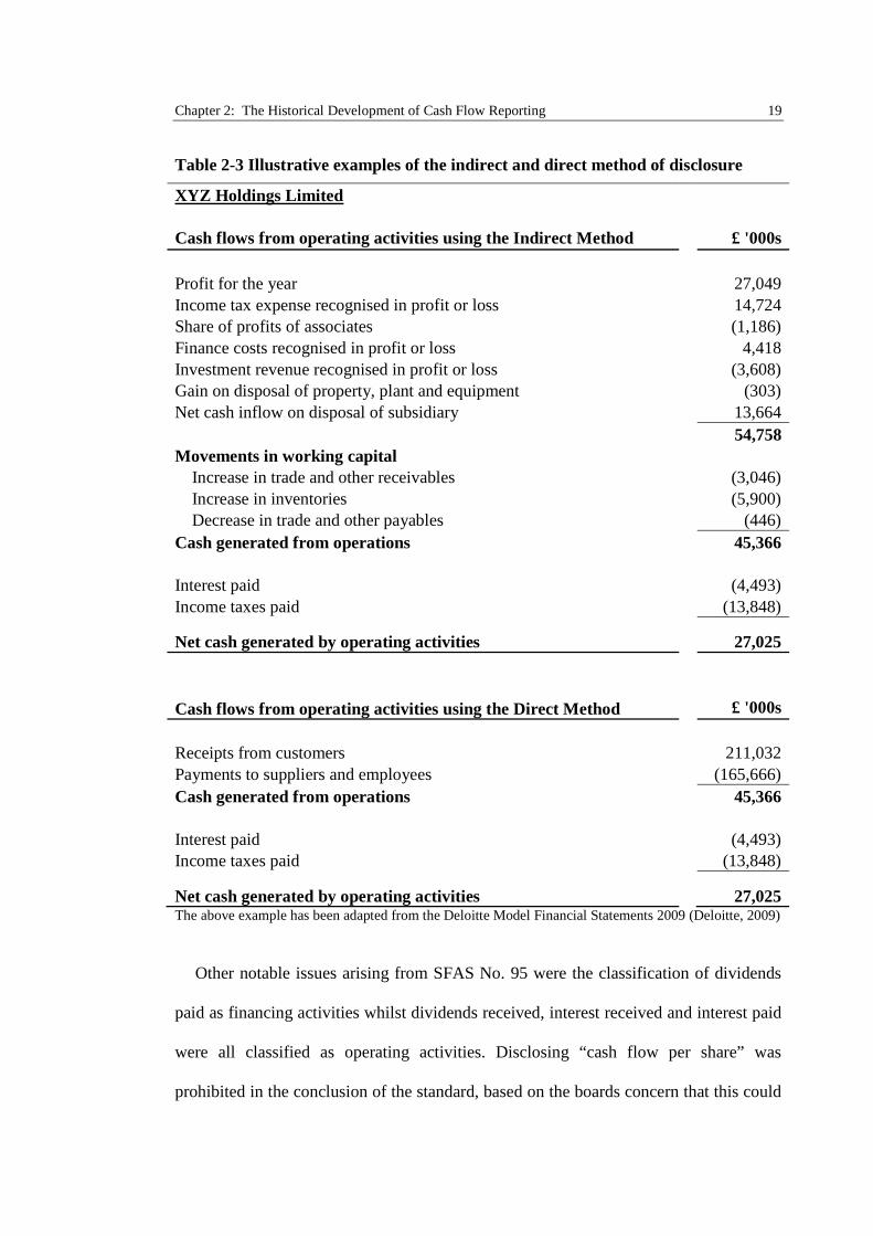
is commonly known as the direct method of cash flow presentation.5 One of the most
fiercely debated topics in cash flow reporting, has arisen from the standard setters’
preference for this approach over the indirect method. This essentially forms the core of
the thesis, which aims to examine the usefulness of direct cash flow statements further.
5 See Table 2-3 for an example of operating cash flows reported using both the direct method and indirectmethod of presentation.
Chapter 2: The Historical Development of Cash Flow Reporting 19
Table 2-3 Illustrative examples of the indirect and direct method of disclosure
XYZ Holdings Limited
Cash flows from operating activities using the Indirect Method £ '000s
Profit for the year 27,049
Income tax expense recognised in profit or loss 14,724Share of profits of associates (1,186)
Finance costs recognised in profit or loss 4,418
Investment revenue recognised in profit or loss (3,608)Gain on disposal of property, plant and equipment (303)
Net cash inflow on disposal of subsidiary 13,664
54,758Movements in working capital
Increase in trade and other receivables (3,046)
Increase in inventories (5,900)Decrease in trade and other payables (446)
Cash generated from operations 45,366
Interest paid (4,493)
Income taxes paid (13,848)
Net cash generated by operating activities 27,025
Cash flows from operating activities using the Direct Method £ '000s
Receipts from customers 211,032
Payments to suppliers and employees (165,666)
Cash generated from operations 45,366
Interest paid (4,493)Income taxes paid (13,848)
Net cash generated by operating activities 27,025The above example has been adapted from the Deloitte Model Financial Statements 2009 (Deloitte, 2009)
Other notable issues arising from SFAS No. 95 were the classification of dividends
paid as financing activities whilst dividends received, interest received and interest paid
were all classified as operating activities. Disclosing “cash flow per share” was
prohibited in the conclusion of the standard, based on the boards concern that this could
Chapter 2: The Historical Development of Cash Flow Reporting 20
mislead shareholders in believing it to be an alternative measure of performance to
earnings per share (FASB, 1987, paragraphs 122-125).
Both The Financial Reporting Council (FRC) in the U.K. and the Australian
Accounting Standards Board (AASB) were quick to follow the U.S. by issuing their
respective standards, Financial Reporting Standard (FRS) 1 in September 1991, and
AASB 1026 in December 1991. Around the same time the International Accounting
Standards Committee (IASC) issued IAS 7 (revised 1992) “Cash Flow Statements”
which replaced IAS 7 (1977) “Statement of Changes in Financial Position” thereby
aligning the IASC more closely with FASB. The next three sections of this chapter will
therefore examine and discuss the development of cash flow reporting in the U.K.,
Australia and by the IASB.
2.3 The Development of Cash flow reporting in the U.K.
2.3.1 The Development of Funds Flow Reporting in the U.K.
The historical development of cash flow reporting in the U.K. followed a very similar
pattern to the U.S., with one noteworthy exception, U.K. firms were a lot slower in their
mass acceptance and use of the funds flow statement.6 Davies et al. (1994), providing
an overview of the history of cash flow reporting in the U.K. up to the issuance of FRS
1, comment that prior to the 1970’s there was little evidence of the same widespread use
of the funds flow statement in the U.K. compared to what had been observed in
America. However, much like in America, Rosen and Don (1969) noted that a form of
funds flow statement had been used by some U.K. companies from as early as 1862.
6See Table 2-4 for an overview of the historical development of cash flow reporting in the U.K.
Chapter 2: The Historical Development of Cash Flow Reporting 21
Table 2-4 Summary of the development of cash flow reporting in the U.K.
Key Date Key Development
1974, April Issue of Exposure Draft (ED) 13: Statements of Source andApplication of Funds for comment
1975, July Issue of Statement of Accounting Practice (SSAP) 10:Statements of Source and Application of Funds effective forfiscal years ending on or after 1 January 1976
1978, June Part 4 added to SSAP 10 highlighting the alignment of thestandard with IAS 7: Statement of Changes in FinancialPosition
1990, July Issue of ED 54: Cash flow statements issued by the ASC forcomment
1991, September Issue of Financial Reporting Standard (FRS) 1: Cash FlowStatements by the Accounting Standards Board (ASB) tosupersede SSAP 10 effective for fiscal years ending on or after23 March 1992
1994, March Issue of Financial Reporting Exposure Draft (FRED) 10:Revision of FRS 1 Cash Flow Statements for comment
1996, October Issue of FRS 1 (Revised 1996): Cash Flow Statements by theASB effective for fiscal years ending on or after 23 March 1997
2002, July Issue of Regulation (EC) No 1606/2002 of the EuropeanParliament and of the Council requires that the consolidatedaccounts of all listed European firms be prepared in accordancewith International Financial Reporting Standards (IFRS)
2005, January The application of IFRS including IAS 7 becomes mandatoryfor all consolidated accounts of listed U.K. companies withannual reporting periods on or after this date
Based on FRS 1 (1991), Davies et al. (1994), FRS 1 (1996), Cox and Pendersen (2002), and Rutherford(2007).
By the 1970’s, however, the Institute of Chartered Accountants in England and
Wales (ICAEW) surveys of published accounts show rapid acceptance and common use
of the funds flow statement within U.K. companies. While only 13% of firms reported a
funds flow statement in 1970, this had risen to 100% by 1979 (Rutherford, 2007, page
Chapter 2: The Historical Development of Cash Flow Reporting 22
82). Driving the quick adoption of funds flow statements was the initial issue of
Exposure Draft (ED) 13 “Statements of Source and Application of Funds” in April
1974 from the recently formed Accounting Standards Steering Committee (ASSC).7 ED
13 offered U.K. companies guidance on how to disclose a funds flow statement, and
received widespread support that resulted in the issuance of SSAP 10 “Statements of
Source and Application of Funds” in July 1975, fifteen months later. SSAP 10 targeted
all enterprises with turnover or gross income greater than £25,000 per annum and
argued that companies should adopt it if their accounts were to provide a “true and fair
view of financial position and profit or loss” (ICAEW, 1985, page 219; paragraph 9).
Firms were, therefore, pressurised by the ASSC to adopt SSAP 10, since according to
the Companies Act (1967), failing to adopt SSAP 10 could lead to a qualified audit
opinion.8
It was not long, however, before SSAP 10 received similar criticisms to those
levelled against the U.S. equivalent, APB No. 19. One of the standard’s main
weaknesses was its vague objective, which portrayed the funds flow statement as a
reconciliation of the opening balance sheet and current year profits with the closing
balance sheet (Davies et al., 1994). From the standard’s objective it was, therefore,
unclear whether the ASSC anticipated SSAP 10 would provide any new information to
financial statement users. In fact, the objective of SSAP 10 appeared to view the funds
flow statement as a mere “reclassification” of information that was already available to
the reader when it stated that:
7 The ASSC was formed by the ICAEW in 1970 with the purpose of carrying out the objectives of theICAEW Council’s statement of intent as agreed on December 12, 1969 to publish authoritative standards,increase the uniformity of accounting practice and encourage the on-going improvement of accountingstandards (Rutherford, 2007, pages 26 and 31).8 The Companies Act (1967) clearly stated in section 14 that the auditor had to express an opinion as towhether the accounts provided a “true and fair view” of the financial position and performance of theentity.
Chapter 2: The Historical Development of Cash Flow Reporting 23
“The funds statement is in no way a replacement for the profit and loss account
and Balance Sheet although the information which it contains is a selection,
reclassification and summarisation of information contained in those two
statements. The objective of such a statement is to show the manner in which the
operations of a company have been financed and in which its financial
resources have been used…”
(ICAEW, 1985, pg 218; paragraph 2)
Further to these criticisms, were those that noted the inadequate definition of “funds”,
and the lack of guidance to encourage a consistent format of disclosure. The missing
emphasis on “cash” flow in the funds flow statement was demonstrated within the
appendix of general guidance to SSAP 10. For example, an entity issuing shares in
return for an interest in a subsidiary company was recommended to disclose the
transaction as both a “source” and “application” of funds, even though there was no
impact on the firm’s cash resources (ICAEW, 1985, pg 224; example 3).
2.3.2 The Issue of FRS 1 Cash Flow Statements
The lack of clear guidance provided by SSAP 10, coupled with the vague objectives and
poor definition of “funds”, pressurised the ASC for further reforms, resulting in the
issue of Exposure Draft (ED) 54: Cash Flow Statements in July 1990. After receiving
the comments on ED 54, the newly formed Accounting Standards Board (ASB) issued
Financial Reporting Standard (FRS) 1 Cash Flow Statements fourteen months later.
FRS 1 was clearly influenced by SFAS No. 95, issued in the U.S. around four years
prior to its development. From the outset of FRS 1, the ASB made it clear that they had
Chapter 2: The Historical Development of Cash Flow Reporting 24
considered the criticisms levelled against SSAP 10 and there was, accordingly, far less
ambiguity regarding the objective of FRS 1, which clearly stated:
“The objective of the FRS is to require reporting entities…to report on a
standard basis their cash generation and cash absorption for a period.”
(FRS 1, 1991, paragraph 1)
From this definition, it was apparent the ASB had addressed two notable caveats of
SSAP 10. FRS 1 required reporting on a “standard basis”, thereby, eliminating
alternative methods of disclosure, which had previously reduced comparability between
firms. Moreover, the standard had moved away from reporting “funds” flow and
focussed on disclosing the “cash” generated and absorbed during the period.
2.3.2.1 Improved Comparability and Change in Scope
The ASB achieved their objective by mandating a very rigid format for the cash flow
statement under five major categories: “operating activities”, “returns on investments
and servicing of finance”, “taxation”, “investing activities” and “financing”. Strictly
categorising cash flows helped to increase the comparability between enterprises,
thereby, resolving one of the major problems of SSAP 10. Further, the scope of the
standard changed to exempt a far wider range of entities when compared to the simple
£25,000 threshold used by SSAP 10. Changing the scope was largely driven by the
argument that the cost of disclosing a cash flow statement would likely outweigh the
benefits of reporting cash flow information for certain entities (FRS 1, 1991, paragraph
58).
Chapter 2: The Historical Development of Cash Flow Reporting 25
A clear definition of “cash flow” provided by the ASB, further helped to increase the
comparability of cash flow statements between companies. The standard defined “Cash
flow” as an increase or decrease in “cash” or “cash equivalents”, with no reference
made to “funds” or working capital. Moreover, FRS 1 defined “Cash” as cash in hand
and demand deposits while it defined “cash equivalents”, much like SFAS No. 95, as
being “short-term highly liquid investments” convertible into cash without notice and
maturing within three months from the date of issuance, such as treasury bills. These
changes were a vast improvement on the loose definition of “net liquid funds” provided
by SSAP 10 as they helped increase the comparability between cash flow statements.
A further change resulting from the move to FRS 1 concerned the disclosure of
operating cash flows. FRS 1 allowed operating cash flows to be reported on a net or
gross basis on the face of the cash flow statement along with a reconciliation of
operating profit to cash flow to be shown as part of the notes to the accounts (FRS 1,
1991, paragraph 16-17). Reading the explanation to the standard makes it is clear that
the ASB were not lobbying their constituents to use the direct method as hard as FASB
when they presented SFAS No. 95. In fact, the ASB put forward a very balanced debate
on the benefits of disclosing operating cash flows using either the direct or indirect
method (FRS 1, 1991, paragraphs 69-72). Consequently, FRS 1 noted that the direct
method may provide useful information for assessing future cash flows but the indirect
method may be useful to assess the quality and persistence of earnings.9 Even though
four out of six of the illustrative examples in the standard’s appendix made use of the
direct method, the ASB only encouraged the use of this approach when the enterprise
9 The ASB note that the indirect method helps investors assess the quality and persistence of historicalearnings by providing a detailed breakdown of past accrual adjustments that would be useful whenforecasting future earnings or cash flows.
Chapter 2: The Historical Development of Cash Flow Reporting 26
believed the benefits of adopting the direct method would outweigh the associated costs
of obtaining the required information. In either case, the ASB were clear that all firms
adopting FRS 1 should disclose a reconciliation of operating profit to cash flow as part
of the notes to the cash flow statement.
2.3.2.2 The Revision of FRS 1 and Subsequent Issue of FRS 1 (Revised)
With the widespread adoption of FRS 1, the ASB wanted feedback on the standard and,
therefore, issued Financial Reporting Exposure Draft (FRED) 10: Revision of FRS 1
Cash Flow Statements for comment (FRS 1, 1996). Based on the responses received to
FRED 10, the ASB issued a revised standard on cash flow reporting; FRS 1 (revised
1996): Cash Flow Statements. The first key change to the old standard concerned the
definition of “cash flow” since business managers had criticised including “cash
equivalents” as part of “cash flow”. They did not consider investments with a maturity
of less than three months at the date of inception to be “equivalent” to cash in the
running of the enterprise. In view of these comments the ASB revised the definition of
“cash flow” to include only “cash”, meanwhile “cash equivalents”, as defined by the
original FRS 1, were reported under a newly created category, “management of liquid
resources” (FRS 1, 1996, appendix 3.6-3.8).
In addition to this new category, the revised FRS 1 added two more levels of cash
flow classification, increasing the total number of standard headings from five to eight.
FRS 1 (Revised 1996) now split cash flows from investing activities into “capital
expenditure and financial investment” and “acquisitions and disposals”, and created two
new categories, “equity dividends paid” and the aforementioned “management of liquid
resources”.
Chapter 2: The Historical Development of Cash Flow Reporting 27
Finally, the last significant revision to the standard now required the reconciliation of
“net debt” to be disclosed either adjoining the cash flow statement or as a separate note
to the accounts. This helped to provide more detailed information regarding the
“liquidity, solvency and financial adaptability” of the enterprise (FRS 1, 1996, appendix
3.11).
2.3.3 The U.K. Transition to IFRS and its Effect on Cash Flow Reporting
Until the adoption of International Financial Reporting Standards (IFRS) by the U.K. in
2005, and since the issue of FRS 1 (Revised 1996), there were no major changes to cash
flow accounting within the U.K. In July 2002, the issue of Regulation (EC) No
1606/2002 of the European Parliament and of the Council required that all listed
European firms prepare their consolidated accounts in accordance with IFRS for
accounting periods commencing on or after 1 January 2005 (Cox and Pendersen, 2002).
All U.K. listed companies were therefore required to undergo a transition from FRS 1
(Revised 1996) to the IFRS equivalent, IAS 7 Cash Flow Statements.
Significant differences were noted in the reporting of cash flows between U.K.
GAAP and IFRS in a 2005 report by PriceWaterhouseCoopers. Defining “cash flows”
was the most significant difference between the two standards, a legacy from the
revisions that the ASB had made to the original version of FRS 1
(PriceWaterhouseCoopers, 2005). IAS 7 defined “cash flows” as “cash and cash
equivalents” whilst the FRS 1 (Revised 1996) had amended their definition to exclude
“cash equivalents” which were reported under the separate category of “management of
liquid resources”. Much like SFAS No. 95, IAS 7 also required cash flows reported
under the three distinct categories of “operating”, “investing” and “financing” activities
as opposed to the eight stipulated under FRS 1 (Revised 1996). Further, IAS 7 did not
Chapter 2: The Historical Development of Cash Flow Reporting 28
require a separate reconciliation of “net debt” or provide any exemptions to the
application of the standard, thereby extending the scope of cash flow reporting
requirements in the U.K. to many previously exempt firms. Finally, IAS 7 increased the
disclosure requirements for U.K. firms reporting foreign exchange differences,
presenting these separately in the reconciliation of the opening and closing cash and
cash equivalent balances.
2.4 The Development of Cash flow Reporting in Australia
2.4.1 The Development of Funds Flow Reporting in Australia
Australian funds and cash flow reporting followed a similar cycle to that observed in
both the U.S. and U.K., with firms incorporating some form of funds flow statement as
part of their annual accounts by the start of the 1970’s (Donleavy, 1994, page 98).10 In
January 1971, the Institute of Chartered Accountants in Australia (ICAA) initially
recommended funds flow reporting by issuing Technical Bulletin F1: “The Funds
Statement”. However, funds flow statements only became widespread after the
Australian Associated Stock Exchanges amended their listing rules in 1972 to mandate
all public companies file one as part of their annual accounts (Walker and Robinson,
1994).11
10 See Table 2-5 for a summary of the development of cash flow reporting in Australia.11 The Australian Associated Stock Exchanges was the predecessor to the Australian Stock Exchange(ASX).
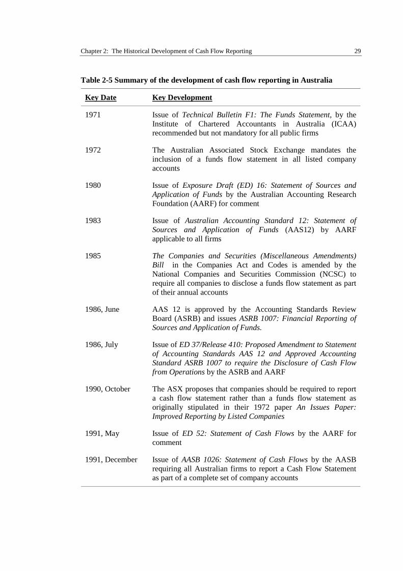
Chapter 2: The Historical Development of Cash Flow Reporting 29
Table 2-5 Summary of the development of cash flow reporting in Australia
Key Date Key Development
1971 Issue of Technical Bulletin F1: The Funds Statement, by theInstitute of Chartered Accountants in Australia (ICAA)recommended but not mandatory for all public firms
1972 The Australian Associated Stock Exchange mandates theinclusion of a funds flow statement in all listed companyaccounts
1980 Issue of Exposure Draft (ED) 16: Statement of Sources andApplication of Funds by the Australian Accounting ResearchFoundation (AARF) for comment
1983 Issue of Australian Accounting Standard 12: Statement ofSources and Application of Funds (AAS12) by AARFapplicable to all firms
1985 The Companies and Securities (Miscellaneous Amendments)Bill in the Companies Act and Codes is amended by theNational Companies and Securities Commission (NCSC) torequire all companies to disclose a funds flow statement as partof their annual accounts
1986, June AAS 12 is approved by the Accounting Standards ReviewBoard (ASRB) and issues ASRB 1007: Financial Reporting ofSources and Application of Funds.
1986, July Issue of ED 37/Release 410: Proposed Amendment to Statementof Accounting Standards AAS 12 and Approved AccountingStandard ASRB 1007 to require the Disclosure of Cash Flowfrom Operations by the ASRB and AARF
1990, October The ASX proposes that companies should be required to reporta cash flow statement rather than a funds flow statement asoriginally stipulated in their 1972 paper An Issues Paper:Improved Reporting by Listed Companies
1991, May Issue of ED 52: Statement of Cash Flows by the AARF forcomment
1991, December Issue of AASB 1026: Statement of Cash Flows by the AASBrequiring all Australian firms to report a Cash Flow Statementas part of a complete set of company accounts
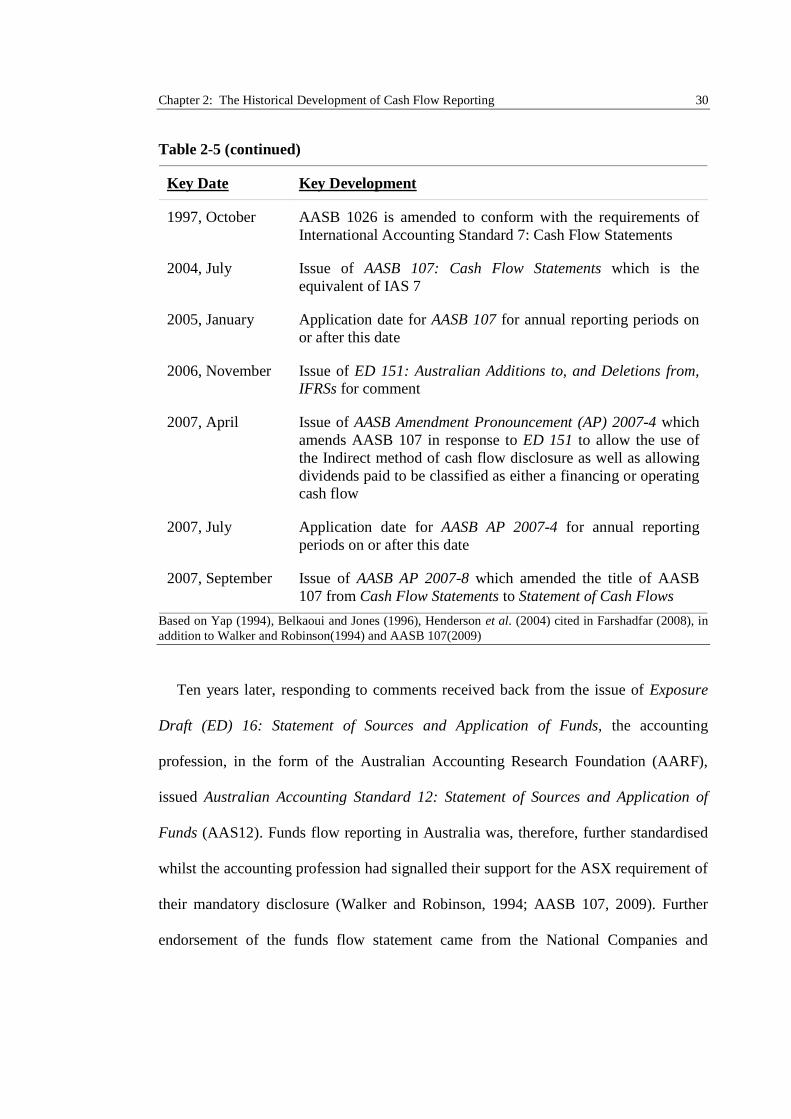
Chapter 2: The Historical Development of Cash Flow Reporting 30
Table 2-5 (continued)
Key Date Key Development
1997, October AASB 1026 is amended to conform with the requirements ofInternational Accounting Standard 7: Cash Flow Statements
2004, July Issue of AASB 107: Cash Flow Statements which is theequivalent of IAS 7
2005, January Application date for AASB 107 for annual reporting periods onor after this date
2006, November Issue of ED 151: Australian Additions to, and Deletions from,IFRSs for comment
2007, April Issue of AASB Amendment Pronouncement (AP) 2007-4 whichamends AASB 107 in response to ED 151 to allow the use ofthe Indirect method of cash flow disclosure as well as allowingdividends paid to be classified as either a financing or operatingcash flow
2007, July Application date for AASB AP 2007-4 for annual reportingperiods on or after this date
2007, September Issue of AASB AP 2007-8 which amended the title of AASB107 from Cash Flow Statements to Statement of Cash Flows
Based on Yap (1994), Belkaoui and Jones (1996), Henderson et al. (2004) cited in Farshadfar (2008), inaddition to Walker and Robinson(1994) and AASB 107(2009)
Ten years later, responding to comments received back from the issue of Exposure
Draft (ED) 16: Statement of Sources and Application of Funds, the accounting
profession, in the form of the Australian Accounting Research Foundation (AARF),
issued Australian Accounting Standard 12: Statement of Sources and Application of
Funds (AAS12). Funds flow reporting in Australia was, therefore, further standardised
whilst the accounting profession had signalled their support for the ASX requirement of
their mandatory disclosure (Walker and Robinson, 1994; AASB 107, 2009). Further
endorsement of the funds flow statement came from the National Companies and
Chapter 2: The Historical Development of Cash Flow Reporting 31
Securities Commission (NCSC) when, in 1985, they amended the statutory rules to
require all companies disclose a funds flow statement with their filed accounts.
Prior to 1985, the AARF largely developed and issued Australian Accounting
Standards without any independent regulatory oversight. Regulation of Australian
Accounting Standards only started once the Accounting Standards Review Board
(ASRB) was formed in 1985 with the mandate to review all the standards issued by the
AARF (Walker and Robinson, 1994). One of the first standards reviewed and issued by
the ASRB was when they initially endorsed AAS 12 in 1986 and subsequently issued
ASRB 1007: Financial Reporting of Sources and Application of Funds.
Conflicts between the ASRB and the AARF significantly slowed the transition from
funds flow reporting to cash flow reporting in Australia (Walker and Robinson, 1994).
SFAS 95 had found favour with the ASRB who were pushing to move away from the
funds flow statement and adopt an entirely new method of cash flow reporting.
Meanwhile, however, the AARF were content to retain the funds flow statement with
modification. Ultimately, the development of cash flow reporting in America, and the
1987 Australian stock market crash, prompted increased pressure from analysts and the
public for significant reforms in accounting and auditing (Walker and Robinson, 1994).
Reforms were, however, slow as the ASRB and the AARF were still at a deadlock over
whether or not to issue a cash flow reporting standard equivalent to SFAS No. 95.
2.4.2 The Development of Cash Flow Reporting in Australia
In response to this deadlock, the ASX intervened yet again and announced in October
1990 that if the ASRB issued an equivalent standard to SFAS No. 95 within the
succeeding two years, they would require all listed companies to disclose a statement of
cash flows by June 30, 1992 (Walker and Robinson, 1994). Responding to the ASX and
Chapter 2: The Historical Development of Cash Flow Reporting 32
the growing demand for cash flow information, the AARF presented their Exposure
Draft 52 Statement of Cash Flows in May 1991 and received overwhelming approvals
from 96% of the respondents (Walker and Robinson, 1994). In December of the same
year, the Australian Accounting Standards Board (AASB) issued AASB 1026 Statement
of Cash flows which became effective by the ASX deadline.12 SFAS No. 95 clearly
influenced AASB 1026, which required cash flows be disclosed under the same three
main headings of “operating”, “investing” and “financing” activities, in addition to
defining “cash equivalents” as:
“...highly liquid investments which are readily convertible to cash on hand...”
(AASB 1026, 1991, paragraph 10)
Disclosing operating cash flows was, however, the significant difference between
AASB 1026 and SFAS No. 95. According to AASB 1026 (1991) paragraph 38-39, an
entity complying with the standard would be required to present their operating cash
flows using the direct method, with a note to the accounts reconciling operating profits
and cash flows. Australia did not allow firms to report operating cash flows using the
indirect method, although this was already used in the U.S. and U.K.
2.4.3 The Australian Transition to IFRS
Australia harmonised their cash flow reporting requirements with IAS 7, in March 1997,
when the AASB issued Exposure Draft 77, followed in October 1997 by the issue of a
revised AASB 1026. Consequently, Australia were far more prepared for the transition
to IFRS than the U.K. as there were only minor notable differences between AASB
12 The Australian Accounting Standards Board was formally known as the ASRB.
Chapter 2: The Historical Development of Cash Flow Reporting 33
1026 and IAS 7, which concerned the disclosure of operating cash flows (Deloitte,
2005). Although IAS 7 encouraged the use of the direct method, the standard provided a
choice between either the direct or the indirect method, so long as firms consistently
applied the chosen approach from one period to the next. AASB 1026, on the other
hand, only permitted constituents to use the direct method of disclosing operating cash
flows and, much like SFAS No. 95, also required a reconciliation of operating profit to
cash flow as part of the notes to the accounts. Classification of dividends paid was
another difference between the two standards. Under IAS 7, dividends paid could be
classified under either operating or financing activities, while AASB 1026 explicitly
required their disclosure as part of the cash flows from financing activities.
Historically, the AASB had required operating cash flow disclosures under the direct
method alone. When adopting IFRS, therefore, they issued their own standard on cash
flow reporting in the form of AASB 107 Cash Flow Statements on July 15, 2004, and
maintained their historical position. AASB 107 was equivalent to IAS 7 in all material
respects, except it did not allow firms to disclose operating cash flows using the indirect
method.
In April 2007, however, in order to align themselves more fully with IFRS, the
AASB amended AASB 107 to permit Australian firms to choose between the two
approaches. AASB Amendment Pronouncement (AP) 2007-4 amended AASB 107 in
response to ED 151, and allowed the use of the indirect method, in addition to requiring
the classification of dividends paid as either financing or operating cash flows.
Chapter 2: The Historical Development of Cash Flow Reporting 34
2.5 The Development of Cash flow Reporting by the IASC/IASB
2.5.1 The Development of Funds Flow Reporting by the IASC
Regulation of funds flow reporting in the U.S. and U.K. prompted the newly formed
International Accounting Standards Committee (IASC) to issue Exposure Draft (ED) 7
in June 1976 on the subject.13 Both the preparers and users of financial statements had
already become accustomed to the funds flow statement, so it was unsurprising that
comment letters received back for ED 7 showed strong support for the new standard
(Camfferman and Zeff, 2007). As a result, in October 1977, the International
Accounting Standards Board (IASB) issued IAS 7 Statement of Changes in Financial
Position, closely following the proposed guidelines laid down by ED 7. However,
similar problems experienced in the U.S. and the U.K. occurred with the adoption of
IAS 7. The definition of “funds” was vague, arising from what appeared to be a
compromise reached by the members of the IASC, of being either “cash”, “working
capital” or “all financial resources” (Taylor, 1987).
2.5.2 The Issue of IAS 7 “Cash Flow Statements”
Much like FASB and the ASB, the IASC realised they needed to address the problems
associated with funds flow reporting and, therefore, they issued Exposure Draft (ED) 36:
Cash Flow Statements in July 1991 for public comment. Seventeen months later, they
followed up ED 36 and issued IAS 7 Cash Flow Statements, effective for all financial
years ending on or after 1 January 1994.
13 See Table 2-6 for a summary of funds and cash flow regulation by the IASC.
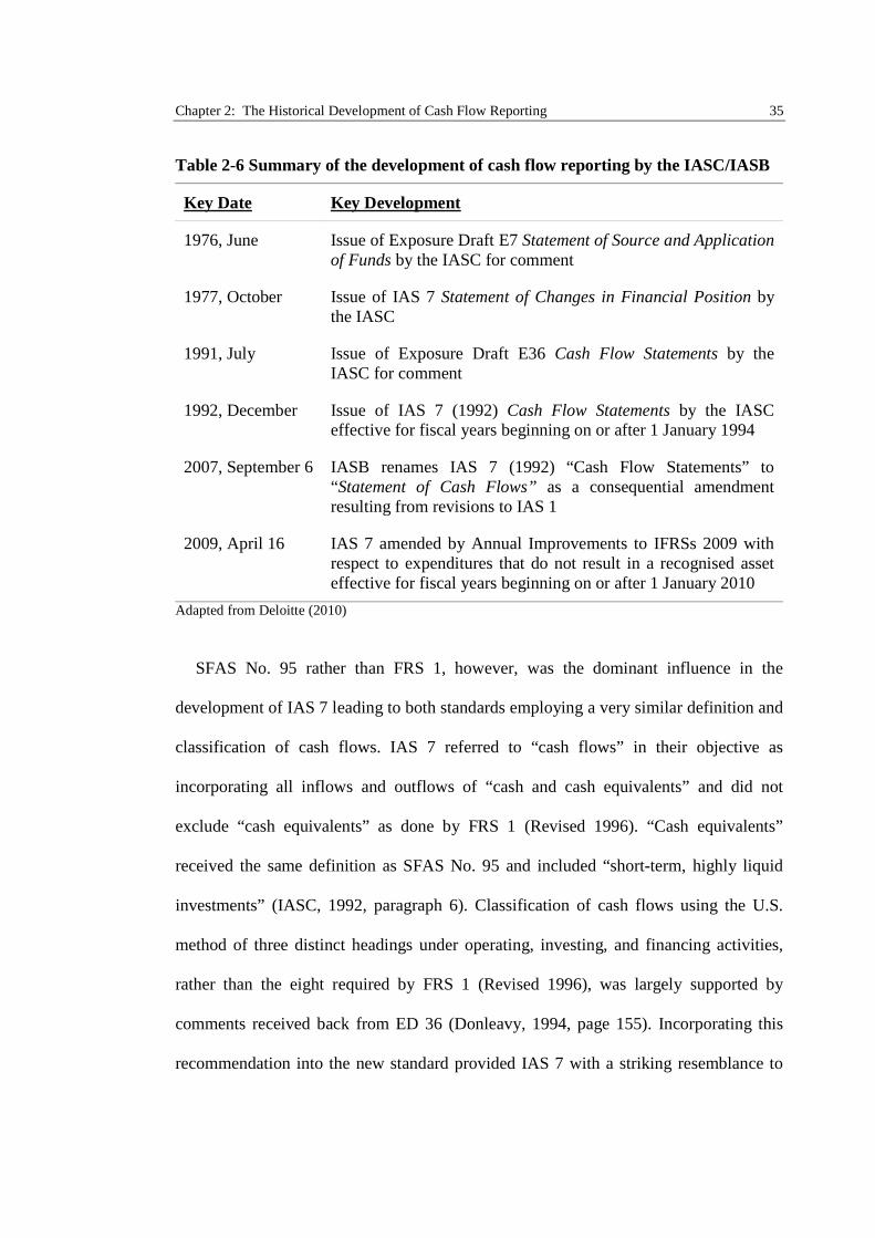
Chapter 2: The Historical Development of Cash Flow Reporting 35
Table 2-6 Summary of the development of cash flow reporting by the IASC/IASB
Key Date Key Development
1976, June Issue of Exposure Draft E7 Statement of Source and Applicationof Funds by the IASC for comment
1977, October Issue of IAS 7 Statement of Changes in Financial Position bythe IASC
1991, July Issue of Exposure Draft E36 Cash Flow Statements by theIASC for comment
1992, December Issue of IAS 7 (1992) Cash Flow Statements by the IASCeffective for fiscal years beginning on or after 1 January 1994
2007, September 6 IASB renames IAS 7 (1992) “Cash Flow Statements” to“Statement of Cash Flows” as a consequential amendmentresulting from revisions to IAS 1
2009, April 16 IAS 7 amended by Annual Improvements to IFRSs 2009 withrespect to expenditures that do not result in a recognised asseteffective for fiscal years beginning on or after 1 January 2010
Adapted from Deloitte (2010)
SFAS No. 95 rather than FRS 1, however, was the dominant influence in the
development of IAS 7 leading to both standards employing a very similar definition and
classification of cash flows. IAS 7 referred to “cash flows” in their objective as
incorporating all inflows and outflows of “cash and cash equivalents” and did not
exclude “cash equivalents” as done by FRS 1 (Revised 1996). “Cash equivalents”
received the same definition as SFAS No. 95 and included “short-term, highly liquid
investments” (IASC, 1992, paragraph 6). Classification of cash flows using the U.S.
method of three distinct headings under operating, investing, and financing activities,
rather than the eight required by FRS 1 (Revised 1996), was largely supported by
comments received back from ED 36 (Donleavy, 1994, page 155). Incorporating this
recommendation into the new standard provided IAS 7 with a striking resemblance to
Chapter 2: The Historical Development of Cash Flow Reporting 36
SFAS No. 95. There were, however, some notable differences between these two
standards concerning the disclosure of operating cash flows, interest and dividends.
Comments received on ED 36 were varied on the method of reporting operating cash
flows. Only one third of respondents to ED 36 favoured the mandatory use of the direct
method, with more than half the respondents preferring to allow a choice between either
the direct or the indirect method (Donleavy, 1994, page 155). IAS 7, therefore,
encouraged the use of the direct method while, at the same time, providing firms with
the choice of using either the direct or the indirect method. Departing from the
requirements of SFAS No. 95, however, the standard did not require firms to show a
reconciliation between operating profit and cash flow if they chose the direct method.
Unlike SFAS No. 95, compelling firms to prepare this reconciliation was seen by the
IASC as a “disincentive” to adopting the direct method (Donleavy, 1994, page 155).
The other significant differences between SFAS No. 95 and IAS 7 concerned the
classification of interest and dividends. IAS 7, paragraph 31, permitted interest and
dividends to be classified either under “operating”, “investing” or “financing” activities,
so long as the chosen approach was applied consistently from one period to the next.
FASB, however, argued that operating cash flows should reflect the “cash effects of
transactions...that enter into the determination of net income” (FASB, 1987, paragraph
88). Thus, SFAS No. 95 only permitted the classification of interest received and paid
and dividends received under “operating” activities, while classifying dividends paid as
“financing” activities.
Subsequent to the issuance of IAS 7 in December 1992, there were largely minor
amendments to the original standard at the time of writing this thesis. In September
2007, the IASB renamed IAS 7 “Cash Flow Statements” to “Statement of Cash Flows”.
Chapter 2: The Historical Development of Cash Flow Reporting 37
More recently, effective for financial years ending on or after 1 January 2010, the IASB
amended IAS 7 to require the disclosure of capital expenditure under investing activities
for only those amounts resulting in the recognition of assets (IASB, 2010).
2.6 The FASB and IASB Convergence Project
SFAS No. 95, and the IASB equivalent, IAS 7, are very similar in a number of areas
largely due to the significant influence the U.S. standard setters have had on the IASB.
In September 2002, subsequent to the issuance of their respective standards on cash
flow reporting, both FASB and the IASB entered into the Norwalk Agreement, and
committed towards the convergence of U.S. GAAP and IFRS. As part of the
convergence process, in October 2008, the IASB and FASB issued a discussion paper
for comments on their preliminary views of financial statement preparation (IASB,
2008). Included in this paper, section 3.70-3.83 provided a detailed proposal for a new
standard to regulate the disclosure of cash flows.
Besides recommending that “cash flows” should be defined as movements in “cash”
only, and not “cash equivalents” (IASB, 2008, paragraph 3.72), there was no surprise
that once again the major area of debate concerned the disclosure of operating cash
flows. The discussion paper’s proposal to mandate the direct method of reporting
operating cash flows, once again, brought up the debate of whether or not to provide a
choice of using either the direct or the indirect method (IASB, 2008, paragraphs 3.75-
3.83). Further, the paper proposes a line by line reconciliation between the statement of
cash flows and the statement of comprehensive income, as opposed to simply
reconciling operating income and cash flows, as currently required (IASB, 2008,
paragraph 3.80).
Chapter 2: The Historical Development of Cash Flow Reporting 38
Improving the level of understanding concerning the relationship between line items
on the statement of cash flows, the statement of comprehensive income, and financial
position, is a key motive behind the proposed changes to cash flow reporting. The paper
argued that the indirect method has a major deficiency due to the lack of disclosure of
any of the major operating cash flow components of cash receipts or payments for the
period. Operating cash flows reported using the indirect method were likened to
reporting the profit or loss for the period by adjusting the annual change in shareholders’
equity for the effects of dividend payments and share movements. While such an
approach would arrive at the total profit or loss, this method would not reveal a vast
amount of useful information for the users of the financial statements (IASB, 2008,
paragraph 3.77).
In contrast, the discussion paper argues that disclosing operating cash flows using the
direct method more consistently achieves the objectives of financial statement
presentation. Examples of such objectives include “cohesiveness”, “enabling users to
assess the timing, amount and uncertainty of future operating cash flows”, and
“providing useful information regarding the entities liquidity and financial flexibility”.
The IASB and FASB considered the assertions regarding the advantages of the indirect
method inadequate compared to the benefits of reporting actual operating cash receipts
and payments under a directly prepared cash flow statement. Concluding the discussion
paper, the FASB and IASB expressed their view that while there are arguments
concerning the costs and benefits of implementing systems to report direct cash flows,
these costs would most likely be a one-off outlay.
Two hundred and twenty nine public comments were received back from the
discussion paper as shown by FASB (2009). Sampling the comment letters from the big
Chapter 2: The Historical Development of Cash Flow Reporting 39
four accounting firms provides interesting insight into the view of the accounting
profession regarding the proposed changes to cash flow reporting. Deloitte, KMPG and
EY all highlighted the need for the IASB and FASB to further investigate whether the
benefits of reporting direct cash flows would indeed outweigh the costs of changing and
implementing financial reporting systems to capture the required information (FASB,
2009, comment letters 63, 114 and 99). PriceWaterhouseCoopers, on the other hand,
showed strong support for mandating the direct method as proposed in the discussion
paper. They did, however, highlight that the level of detail proposed by the discussion
paper may be excessive (FASB, 2009, comment letters 172).
In response to the comment letters, a rough version of the FASB Exposure Draft on
Financial Statement Presentation issued on July 1, 2010 revealed very little change from
the initial discussion paper. With the exception of requiring a less detailed
reconciliation to support the direct cash flow statement, the FASB and IASB has made
no notable changes. The proposed mandatory use of the direct method was still clearly
evident in the Exposure Draft (FASB, 2010, paragraphs 168-199). Changing
information systems, or indirectly adjusting the statement of comprehensive income and
financial position for accruals and other non-cash transactions, were the two
recommended methods of obtaining the necessary information to disclose direct cash
flows.
2.7 Summary and Conclusion
Cash flow reporting is, historically, the oldest form of accounting for transactions,
dating back to medieval times. However, it was not until 1963 that the APB in the U.S.
issued the first standard to govern the reporting of cash flows in the form of Opinion No.
Chapter 2: The Historical Development of Cash Flow Reporting 40
3 “The Statement of Source and Application of Funds”. Australia and the U.K. followed
suit around ten years later and issued Technical Bulletin F1: The Funds Statement in
1971 and SSAP 10: Statements of Source and Application of Funds in 1975 respectively.
Since their inception, similar problems plagued the various funds flow standards,
with the main issues concerning the very vague definition of “funds” and the lack of
clear guidance in their application. Addressing these problems, the standard setters in
America, U.K. and Australia all issued superseding “cash” flow disclosure requirements
towards the end of the 1980’s and start of the 1990’s. America, in the form of SFAS No.
95, having led the way, heavily influenced the standards on cash flow reporting
subsequently issued around the world.
In the 1990’s, U.S., Canada, U.K. and Australia, known as the “G4”, committed to
the harmonisation of accounting standards, along with the International Accounting
Standards Committee (IASC), based on their similar conceptual frameworks (Street and
Shaughnessy, 1998). Towards the end of the 20th century cash flow reporting was an
area in which the G4 and the IASC had clearly gained rapid consensus, resulting in only
minor notable differences between the various standards. More recently, with the
growing acceptance and adoption of IFRS around the world, the U.K. and Australia
have both been reporting their cash flows according to IAS 7. Australia, however,
restricted the choice of disclosing operating cash flows to the direct method until the
issue of AASB Amendment Pronouncement (AP) 2007-4, which amended AASB 107,
thereby allowing the use of the indirect method of cash flow disclosure.
Operating cash flow disclosure is one area in cash flow reporting that has been the
subject of fierce debate by standard setters, preparers and users of financial accounts.
Central to this debate is whether to allow or remove the choice of disclosing operating
Chapter 2: The Historical Development of Cash Flow Reporting 41
cash flows “indirectly” or “directly”. Indirect reporting requires a reconciliation
between profits and net operating cash flow by adjusting for the effects of accrual
accounting and other non-cash transactions. The direct method, however, requires the
disclosure of the actual gross cash receipts and payments on the face of the cash flow
statement, supported with a supplemental “indirect” reconciliation.
Currently, as part of the continuing harmonisation of U.S. standards with IFRS,
both FASB and the IASB have proposed to settle the debate finally by removing the
option to disclose operating cash flows using the indirect method and mandate the direct
method for all companies. Comments received back in response to the Exposure Draft,
entreated the FASB and IASB to reconsider whether the benefits of disclosing operating
cash flows “directly” would exceed the associated costs of capturing and recording the
requisite information. Establishing, therefore, which approach provides more useful
information is not easily resolved.
Chapter 3: Literature Review 42
3Literature Review
3.1 Introduction
Over the past two decades, there has been growing interest concerning the usefulness of
information provided from reporting operating cash flows using the direct method. Even
before the standardisation of cash flow disclosures, a number of academic papers,
examining various reporting formats for operating cash flows, had each expressed a
definitive preference for the direct method (Paton, 1963; Heath, 1978; Lee, 1981;
Thomas, 1982; Ketz and Largay III, 1987).
Before and after the regulation of cash flow reporting, there are three distinct
avenues within which researchers have sought to measure the usefulness of estimated
and reported operating cash flows, in addition to their components. Reviewing the
extant literature up to 1990, investigating the usefulness of operating cash flows, Neill
et al. (1991) summarised the published studies into three categories: the effects of cash
flows on capital markets; their usefulness in forecasting future cash flows; and finally,
their usefulness in predicting corporate failure. However, a crucial area they did not
discuss was the benefits of reporting cash flows using the direct method, due to the lack
of empirical research examining the usefulness of this information.
Surveys and case studies were the two initial methods used to assess the usefulness
of cash flows disclosed using the direct method. Lee (1981) surveyed a group of
Chartered Accountants in Scotland, and found that 80% of respondents were in favour
of the model cash flow statement using the direct method provided in the paper.
Moreover, the remaining respondents actually suggested a more detailed presentation of
Chapter 3: Literature Review 43
operating cash flows (OCF) would be more useful. By contrast, however, a replication
of this study on a group of U.S. audit partners, shortly after the release of SFAS No. 95,
found that 57% favoured the indirect method (McEnroe, 1989).
Subsequent U.S. surveys, however, contradicted these initial findings, including a
follow up study by McEnroe (1996) with increased sample size and diversity, covering
academics, accountants, analysts and investors. McEnroe (1996) found 56% of
respondents were in favour of reporting OCF using the direct method, a notable shift in
preference from the 1989 results. Further, survey results reported by Smith and Freeman
(1996) using a group of U.S. finance directors in 1993, provided additional support for
the direct method. When compared with the indirect method, most respondents
indicated the direct approach presented more concise, better quality, and understandable
information. They also indicated support for a hybrid form of cash flow reporting,
presenting operating cash flows directly, but also providing a supplementary
reconciliation between the operating profit and cash flow for the period.
Similar surveys conducted in Australia, where direct cash flow statements were
mandatory, provided further support for the direct method (Jones et al., 1995; Jones and
Ratnatunga, 1997; Jones and Widjaja, 1998; Goyal, 2004). Respondents noted, that, the
direct method was easier to understand and analyse and, when compared with the
indirect method, provided information that was useful to forecast future insolvency
more accurately.
More recently, as part of the convergence project between IFRS and U.S. GAAP, the
Institute of Chartered Financial Analysts (CFA Institute) surveyed their members for
opinions on the usefulness of information reported by direct cash flow statements.
Results published in July 2009 show that, out of 541 respondents, 63% either “strongly
Chapter 3: Literature Review 44
agreed” or “agreed” that information provided by the direct method would improve the
accuracy of future cash flow forecasts and be useful to measure earnings quality (CFA
Institute, 2009). Moreover, 94% voted “Revenue collections from customers”,
information only available under the direct method, to be the most important
information disclosed under the cash flows from operating activities.
In addition to these surveys, a few case studies have also investigated the decision
usefulness of information provided by the direct and indirect method. Soon after the
issuance of SFAS No. 95, Klammer and Reed (1990) used a fictitious case of a firm
seeking a $5 million bank loan, in order to examine the differential usefulness of direct
and indirect cash flow statements. After presenting this case to a group of bank analysts
and loan officers, they provided half the group with a direct cash flow statement, and
the remainder with an indirect cash flow statement. Their results show far greater
consistency in the loan size granted between members using the direct cash flow
statement as compared with the members using the indirect cash flow statement.
In a real life scenario, Trout et al. (1993) report that, after providing the bank with a
direct cash flow statement, Chicago Central & Pacific Railroad Company received a
critical loan that helped resolve their liquidity crisis. Management used the direct cash
flow statement to identify the cause of the firm’s cash flow budget variances, enabling a
successful negotiation of a recovery package.
However, in contrast to these case studies, Kwok (2002) reported no participants in
her behavioural study used information provided by the direct method when arriving at
their final lending decision. By using a verbal protocol analysis methodology, she
observed the decision making process of a group of twenty loan officers, analysts,
academics and auditors. None of the subjects noted the difference between the two
Chapter 3: Literature Review 45
methods of disclosing cash flows. Rather, they based their final lending decisions on
information from the balance sheet and notes and derived any cash flow information
indirectly.
3.2 Empirically Examining the Usefulness of Operating Cash Flows
The survey results and case studies findings highlight that users and preparers of
financial accounts generally prefer the direct method. Unsurprisingly, therefore,
standard setters’ have promoted this approach ahead of the indirect method. However,
the decisions by the FASB, FRC and IASC to allow the indirect method as an
alternative, has motivated many papers to examine the comparative usefulness of these
two options.
Prior to the empirical studies investigating the usefulness of direct cash flows, Neill
et al. (1991) summarised the initial literature examining the usefulness of aggregate
operating cash flows. Studies were categorised into three broad fields of those
examining the usefulness of cash flows in predicting future cash flows and earnings,
explaining capital market effects, and predicting corporate failure. Using the former two
classifications, the next subsections extend the literature review by providing an
overview of the research investigating the usefulness of reporting direct operating cash
flows.
3.2.1 Using Cash Flow Data to Forecast Future Cash Flows and Earnings
An assertion FASB made in their Statement of Financial Accounting Concepts (SFAC)
No. 1, motivated the initial empirical papers examining the usefulness of aggregate
operating cash flows. Information from accrual accounting was claimed to provide a
superior basis for estimating future cash flows when compared with the information
Chapter 3: Literature Review 46
from the historical cash receipts and payments (FASB, 1978, paragraph 9). Since SFAS
No. 95 only became effective from July 1988, the initial papers testing this assertion
estimated the value of operating cash flows used as the dependent variable. Questions
were raised, however, concerning the findings based on estimated proxies for operating
cash flows rather than the actual amounts reported in the cash flow statement (e.g.,
Austin and Bradbury, 1995; Mitchell et al., 1995; Bahnson et al., 1996; Hribar and
Collins, 2002). By estimating operating cash flows from data after the standardisation of
cash flow reporting, results showed significant differences between these proxies and
the actual reported values. It is imperative, therefore, to differentiate between studies
using proxies for operating cash flows and those using reported operating cash flows.
Bowen et al. (1986), Greenberg et al. (1986), Lorek et al. (1993), Finger (1994),
Lorek and Willinger (1996), and Dechow et al. (1998) all examined the usefulness of
operating cash flows to forecast future cash flows by using estimated proxies for
operating cash flows. Greenberg et al. (1986) and Bowen et al. (1986) provided two of
the first papers which empirically tested the FASB assertion that earnings were superior
to cash flows in forecasting future cash flows. Both of these papers used parsimonious
cross-sectional models that employed either total earnings or total operating cash flows
as explanatory variables. Greenberg et al. (1986) compared the ability of historical
earnings and cash flows to predict cash flows for up to five years. Comparing the
coefficients for each regression, their results supported the assertion that earnings
provided a better basis to forecast cash flows for all but the fourth year forecast.
In contrast, Bowen et al. (1986) concluded that, based on their model forecasting one
and two year cash flows, their results failed to uphold FASB’s assertion. Pairwise sign
tests, comparing cash flow prediction errors by using either net income or a proxy for
Chapter 3: Literature Review 47
operating cash flows as explanatory variables, revealed no significant difference
between the two models. Rather, the lowest reported forecast errors came from the
models using working capital from operations or net income before depreciation and
amortisation as explanatory variables.
3.2.1.1 Using Time Series Models to Forecast Cash Flows
Using a longer time horizon, Finger’s (1994) results, based on more than 50 firm-year
observations ending in 1987, the year before cash flow reporting became mandatory,
again failed to uphold FASB’s assertion. Unlike previous studies, using cross-sectional
models with one year lagged explanatory variables, Finger (1994) used time series
models with either two years of lagged cash flows or earnings to forecast cash flows for
up to eight years. Comparing the distribution of the root mean squared errors between
the two models, revealed that historical cash flows more accurately forecast future cash
flows for short time horizons, whereas historical earnings and cash flows were
equivalent predictors for longer time horizons.
Both Lorek et al. (1993) and Lorek and Willinger (1996) further examined the
predictive ability of earnings and cash flows by using time series, rather than cross-
sectional models, to control for individual firm variability in the explanatory variables.
Unlike most studies, which used annual earnings and cash flows, they used quarterly
data. Lorek et al. (1993) found that a seasonal univariate autoregressive model yielded
the lowest mean absolute percentage error (MAPE) when compared to other time series
and cross-sectional models predicting operating cash flows. Extending this study, Lorek
and Willinger (1996) found that their multivariate time series prediction model yielded
an even lower MAPE. Their paper was one of the first studies to disaggregate accruals
and incorporate historical accrual components as explanatory variables in a cash flow
Chapter 3: Literature Review 48
forecasting model. Cash flow prediction significantly improved after including the
lagged values of receivables, inventory and payables, providing evidence for FASB’s
high view of the predictive content available from accrual accounting.
Using firm specific time series prediction models based on annual rather than
quarterly data, Dechow et al. (1998) reported further evidence that historical earnings
provided incrementally more predictive information than historical cash flows.
Although their sample spanned both the pre and post SFAS No. 95 reporting period,
they still estimated their proxy for operating cash flows and found that earnings were
consistently more informative than cash flows in forecasting cash flows up to three
years into the future.
3.2.1.2 Disaggregating Earnings and Operating Cash Flows
Most of the studies, up to and including Dechow et al. (1998), examined the
incremental predictive power of earnings versus cash flows by using parsimonious
cross-sectional or time series regression models, with few explanatory variables.
Towards the start of the 21st century, however, the incremental information content
within the components of total earnings and cash flows became an area of growing
interest, resulting in an extension of more complex prediction models. Barth et al.
(2001b) and Krishnan and Largay III (2000) presented two of the first papers that
developed these models, while at the same time using reported rather than estimated
operating cash flows proxies.
Barth et al. (2001b) expanded the model popularised by Dechow et al. (1998) by
disaggregating total earnings into seven major components – changes in accounts
receivable, changes in inventory, changes in accounts payable, depreciation,
amortisation and other accruals – and total operating cash flows. After disaggregating
Chapter 3: Literature Review 49
total earnings into these seven explanatory variables, their results showed an increase in
the predictive model’s goodness of fit, as measured by the adjusted R2. Compared with
models using either total earnings or total cash flows as independent variables, the
model with disaggregated earnings revealed the highest adjusted R2. Overall, these
findings supported FASB’s assertion that total earnings and its “components” would
help improve the prediction of future cash flows more than historical cash flows alone.
In addition to Barth et al. (2001b), Krishnan and Largay III (2000) disaggregated
earnings, but focussed primarily on disaggregating total operating cash flows, in their
cross-sectional cash flow prediction models. They presented the first empirical study to
examine the incremental information content of direct cash flow components in cash
flow prediction models. Since most U.S. firms report operating cash flows under the
indirect method, Krishnan and Largay III (2000) used a restricted sample of 405 firm-
year observations which chose the direct method between 1988-1993. By comparing
two cash flow prediction models - one using the actual reported operating cash flow
components from the direct method, and the other using indirect method variables for
the same firms - they found that using direct cash flow components yielded higher
adjusted R2. Further, following a similar methodology to Lorek and Willinger (1996),
MAPE results were compared across different cash flow prediction models, with and
without incorporating the components from the direct cash flow statement. Including
direct operating cash flow components, however, consistently and significantly
improved the accuracy of the cash flow prediction model, beyond those using aggregate
cash flows alone. Since they were restricted to using a small sample of firms reporting
direct cash flows, Krishnan and Largay III (2000) extended their tests by estimating
direct cash flow components for a far larger sample, finding similar results.
Chapter 3: Literature Review 50
Cheng and Hollie (2008) provide further evidence of the usefulness of direct
operating cash flow components in predicting cash flows, extending Barth et al.’s
(2001b) model by disaggregating total operating cash flows into “core” and “non-core”
components. Their algorithms used to estimate the operating cash flow components
were very similar to those used by Krishnan and Largay III (2000) when they estimated
the direct cash flow components.14 “Core” operating cash flow components included
their estimates for cash receipts from customers, cash paid to suppliers, and cash paid
for operating and administrative expenses, whilst “non-core” operating cash flows
included interest paid, taxes paid, and other operating cash flows. Pair-wise tests of the
difference in coefficients from the annual cross-sectional regressions of a large sample
of U.S. firms showed, that, core operating cash flow components persisted more highly
into future cash flows than non-core operating cash flow components. Comparing the
adjusted R2 of all their models, their results showed the highest adjusted R2 for the
model using disaggregated operating cash flows and aggregate accruals as explanatory
variables, although this model also yielded the highest out of sample prediction error.
However, when using in sample prediction tests, they showed a notable improvement in
cash flow forecast accuracy after disaggregating total cash flows into their component
parts, especially for firms with high cash flow volatility.
By including dividend receipts, as well as the disaggregated components of net
interest as independent variables in their regression, Arthur and Chuang (2008) build on
Cheng and Hollie’s (2008) model. Using a sample of Australian firms, where the direct
14 For example, Cash receipts from customers were calculated as sales less any changes in accountsreceivable. Cash paid to suppliers was calculated by deducting any changes in accounts payable from thecost of goods sold. Cash paid from operating and admin expenses were calculated as operating expensesminus any changes in net operating working capital, excluding changes in trade accounts receivable,inventory, tax payable and interest payable (Cheng and Hollie, 2008).
Chapter 3: Literature Review 51
method of cash flow presentation was mandatory, they produced the first paper to
overcome the sample self-selection bias inherent in prior U.S. studies that used samples
of firms choosing to use the direct method. Moreover, since Australian firms all
reported their operating cash flows according to the direct method, they used actual,
rather than estimated, direct cash flows for their explanatory variables. Comparing the
respective adjusted R2 of their annual cross-sectional models their findings showed the
highest explanatory power when operating cash flows were disaggregated into their
direct components. Moreover, they found the components of “Cash receipts from
customers” and “Cash payments to suppliers and employees” were significant in
predicting future operating cash flows across all their regressions.
Using a far larger sample of 3,672 firm-year observations from Australian listed
companies between 1992 and 2005, Arthur et al. (2010) further examine the
incremental benefits of reporting direct cash flow components. However, in contrast
with prior studies, Arthur et al. (2010) examined and compared the ability of net and
gross direct cash flows to forecast future earnings, rather than future cash flows. Results
from both their pooled and annual cross-sectional models revealed higher explanatory
power, as measured by the adjusted R2, when using disaggregated direct cash flows
compared to aggregate operating cash flows as independent variables. Moreover, their
results show that a higher disaggregation of operating cash flows resulted in a lower
MAPE and therefore a higher predictive accuracy of future earnings. Following Cheng
and Hollie (2008), and classifying cash flows into core and non-core components, they
further noted that the model with “core” cash flows along with disaggregated “non-core”
components persisted more highly into future earnings, than the model with aggregate
cash flows. Combining cash receipts and payments into “core” cash flows, however,
Chapter 3: Literature Review 52
yielded almost the same explanatory power as disaggregating “core” cash flows into
“cash received from customers” and “cash paid to suppliers and employees.”
Orpurt and Zang (2009) also examined the predictive value of direct cash flow
components to forecast future cash flows and earnings. Conducting their research in the
U.S., their sample of 470 firm-year observations was restricted to entities employing the
direct cash flow method from 1989-2002. To examine whether direct cash flows were
incrementally informative to indirect cash flows, they calculated “articulation errors”
for their sample of firms. Articulation errors are the difference between the reported
direct cash flows and those estimated from the financial information available in the
income statements, balance sheets, and indirect cash flow statements. By adjusting their
estimated direct cash flows for these articulation errors, they were able to examine
whether there was a significant difference between the predictive abilities of actual and
estimated direct cash flows. Including the articulation errors as independent variables
resulted in a significant increase in the explanatory power of the predictive models,
providing further evidence to support the usefulness of the information content found
within the components of a direct cash flow statement.
Recently, however, Lorek and Willinger (2009) criticised these multivariate cash
flow prediction models which show increased explanatory power after disaggregating
earnings or cash flows. They provide evidence that, although disaggregating earnings
provides a high “goodness of fit” as measured by the adjusted R2, this does not
necessarily lead to an improved out of sample predictive accuracy. Using quarterly data,
and a parsimonious model as was common pre Barth et al. (2001b), they revealed a
significantly lower MAPE for their out of sample predictive tests than when using the
more complex model as popularised by Barth et al. (2001b). Lorek and Willinger (2009)
Chapter 3: Literature Review 53
also found that a time series model, rather than cross-sectional regression models,
resulted in the highest increased out of sample predictive accuracy as they were able to
better control for individual firm variability in the explanatory variables. Farshadfar and
Monem (2013) and (2012) use both in and out of sample predictive tests to examine the
usefulness of direct cash flow components to predict future cash flows. Using a sample
of 348 listed Australian firms between 1992 and 2004, they find that disaggregating
operating cash flows into direct cash flow components significantly improves the
accuracy of both the in and out of sample predictive tests.
3.2.2 Using Cash Flow Data to Explain Capital Market Effects
Historical cash flows and earnings provide useful information to help forecast future
cash flows and earnings, when evaluating both future performance and current firm
value. Consequently, a number of studies have examined the association between
market returns and historical cash flows and earnings. Ball and Brown (1968) produced
one of the first seminal papers in this field, empirically examining the association
between accounting numbers in the form of annual net income and company stock
returns. Their findings emphasised the value relevance of historical accounting
information, and demonstrated a strong link between accounting earnings and stock
price movements. By approximating cash flows as equivalent to operating income, Ball
and Brown (1968) further found that net income was superior to their cash flow proxy
when predicting the sign of abnormal stock returns. Extending the work of Ball and
Brown (1968), Beaver and Dukes (1972) examined the information content of different
measures of net income. Once again, changes in net income had the highest association
with abnormal stock returns, as compared with changes in their cash flow proxy
calculated as net income before depreciation, amortisation and deferred taxation.
Chapter 3: Literature Review 54
3.2.2.1 Information Content Studies and Disaggregating Total Earnings
Subsequent research in this area further developed these initial studies by investigating
the incremental information provided by income and cash flow variables when
explaining stock returns. Two of the first such papers were the studies by Patell and
Kaplan (1977) and Beaver et al. (1982). Defining cash flows as working capital, Patell
and Kaplan (1977) found no evidence that percentage changes in cash flows provided
incremental information to earnings when explaining stock returns. Beaver et al. (1982),
however, defined cash flows as net income before depreciation and amortisation, and
found weak evidence that percentage changes in cash flows did provide incremental
information to earnings when explaining annual stock returns. A significant limitation
of these initial papers, however, concerns their definitions for “cash flows”. These
variables were highly correlated with earnings and, when explaining stock returns, were
therefore unlikely to provide incremental information to earnings (Christie et al., 1984).
Following a similar progression to the cash flow prediction literature, capital market
studies also disaggregated total earnings to investigate the information content of these
components when explaining stock returns. Rayburn (1986), Wilson (1986), Wilson
(1987), Bowen et al. (1987), and Bernard and Stober (1989) were some of the first
studies to examine the effect of disaggregating earnings into operating cash flows and
accruals on traditional abnormal stock returns models.
Defining cash flows as earnings before depreciation, amortisation and working
capital movements, Rayburn (1986) found a significant association between abnormal
stock returns, total cash flows and total accruals. While this study did not specifically
compare the information content of cash flows and accruals with total earnings, Wilson
(1986), Wilson (1987), and Bowen et al. (1987) addressed this in their papers. By using
Chapter 3: Literature Review 55
daily stock returns, Wilson (1986) and Wilson (1987) compared the market reaction
between the earnings announcement date and annual report release date. This allowed
them to measure the impact of any incremental information released from reporting the
disaggregated earnings components of accruals and operating cash flows in the latter
report. Their findings show that accruals and operating cash flow components provided
significantly more information than total earnings alone.
Moreover, Bowen et al. (1987), reverting back to an annual event window, found
further evidence that unexpected operating cash flows provided incremental information
content to explain abnormal stock returns beyond aggregate unexpected earnings.
However, Bernard and Stober (1989) failed to find any significant association between
unexpected cash flows and abnormal stock returns when extending Wilson’s (1987)
model over a greater time period, implying that Wilson’s (1987) results may have been
sample specific.
Dechow (1994) further extended the literature by examining the association of
realised, rather than unexpected or abnormal, stock returns with quarterly and annual
earnings and operating cash flows. Compared with prior research, which focussed on
the relative information content of operating cash flows, earnings and accruals, Dechow
(1994) set out to establish which variable provided the single best measure of firm
performance. Given that the sample ended just after the introduction of SFAS No. 95,
cash flows were estimated as operating income before depreciation less interest, taxes,
and non-cash changes in working capital. Results from the cross-sectional regressions
and Vuong (1989) tests show historical earnings to be the superior measure of firm
performance. Providing further evidence of the high association of stock returns with
earnings, Sloan (1996) argued that investors “fixated” on earnings when assessing firm
Chapter 3: Literature Review 56
value, effectively ignoring the information found in the components of total earnings.
Once total earnings were disaggregated into accruals and cash flows, he found that
firms with high/(low) levels of accruals, relative to cash flows in historical earnings,
experienced significantly negative/(positive) future abnormal stock returns.
Disaggregating earnings clearly provided incremental information beyond that available
in total earnings.
3.2.2.2 Disaggregating Operating Cash Flow into the Direct Method Components
Most empirical research examining the capital market effects of the release of earnings
and cash flow information investigated the information content of aggregate earnings,
cash flows and accruals, rather than their disaggregated components. Livnat and
Zarowin (1990), however, presented the first paper which tested the differential
explanatory power of estimated direct cash flow components when explaining market
returns. Their initial findings revealed statistically significant associations between
cumulative abnormal stock returns and the unexpected cash collections from customers,
payments to suppliers and employees, interest payments and other unexpected operating
cash flows. Moreover, analysis of variance tests showed that direct cash flow
components provide incremental information beyond aggregate operating cash flows
when explaining cumulative abnormal stock returns.
Besides Livnat and Zarowin (1990), who estimated their direct cash flow
components, no prior studies had examined whether direct cash flow components
provided incremental information to aggregate operating cash flows when explaining
capital market returns. Addressing this question would provide standard setters with
useful evidence for the debate of whether or not to mandate the direct method of cash
flow reporting. Clinch et al. (2002), therefore, extended Livnat and Zarowin’s (1990)
Chapter 3: Literature Review 57
study by examining a large sample of listed Australian firms from 1992-1997, where
they could use actual, rather than estimated direct cash flows.
Clinch et al. (2002) reported a significantly strong positive association between
annual stock returns and the variables for cash collections from customers and cash paid
to suppliers and employees. Chi-square tests of coefficient equality, however, revealed
that while the disaggregated accruals provided incremental information for all firms,
disaggregating cash flows only provided more information for mining firms. For
industrial firms, disaggregating cash flows did not provide any further information
when explaining stock returns. However, when controlling for the predictive power of
the cash flow components, they found that when direct cash flow components provided
incremental predictive power, they also provided further information to explain stock
returns. Finally, following Livnat and Zarowin (1990), they estimated direct cash flow
components. When comparing the actual and estimated direct cash flows components
across all firms, they found that as the difference between the two increased, the
incremental information provided by the actual direct cash flow components also
increased. Direct cash flow statements, therefore, clearly provided value relevant
information, and more so when more difficult to accurately estimate.
More recently, for a sample of U.S. firms, Orpurt and Zang (2009), in addition to
establishing the usefulness of direct cash flows in forecasting future cash flows and
earnings, examined the capital market effects on firms reporting direct cash flows.
Using dummy variables, they investigated whether stock prices reflected more future
earnings information for firms reporting direct cash flows compared with those using
the indirect method. For firms using the direct method, they demonstrated a strong
correlation between future earnings and current stock returns, as well as between future
Chapter 3: Literature Review 58
operating cash flows and current stock returns. Investors, therefore, could more
accurately forecast earnings for firms reporting direct cash flows, resulting in stock
prices that better reflected future performance expectations, compared with firms
reporting indirect cash flows.
3.3 The Impact of Adopting IFRS
All the most recent studies, to date, examining the usefulness of direct cash flow
reporting, have specifically excluded firm-year observations under IFRS (Arthur et al.,
2010; Farshadfar and Monem, 2012, 2013). Justifying their decision to exclude the
years since Australia adopted IFRS from their sample, Arthur et al. (2010) reason that:
“…from this date, the measurement of both earnings and accruals changed”
(Arthur et al., 2010, page 15).
The potential impact of the mandatory, large-scale, adoption of IFRS received growing
attention when, in July 2002, the European Parliament and Council announced that all
listed European firms must prepare their consolidated accounts using IFRS on or after 1
January 2005. Immediately following this news, the Financial Reporting Council in
Australia also announced that Australian companies would be required to comply with
IFRS by the same deadline.
One of the main objectives of the International Accounting Standards Committee
(IASC) Foundation as defined in their Foundation Constitution is:
Chapter 3: Literature Review 59
“…to develop, in the public interest, a single set of high quality, understandable
and enforceable global accounting standards that require high quality,
transparent and comparable information in financial statements and other
financial reporting to help participants in the world’s capital markets and other
users make economic decisions”
(IASC Foundation, 2009, paragraph 2a)
From this definition, it is clear that the IASC believed that IFRS accounts should
provide information to help users make sound economic decisions given their high
quality, transparency and comparability between firms. Paragraphs 15-18 of the IFRS
reporting framework, further emphasises that the decision usefulness of financial
information is one of the main objective of IFRS (IASB, 1989). Repeated throughout
these paragraphs, in order to meet this objective, is the aim that IFRS accounts should
provide users with information to help evaluate an entity’s future cash generating
potential.
A growing number of studies have empirically tested these assertions, by examining
the economic impact made by IFRS, and the change in reporting quality after either the
voluntary or the mandatory adoption of IFRS, by firms around the world. Armstrong et
al. (2010) presented one of the first papers to reveal investors’ perceptions towards the
adoption of IFRS by analysing European market reactions to 16 separate
announcements between 2002 and 2005, indicating the likelihood of IFRS adoption in
Europe. Investors could interpret the mandatory adoption of IFRS as either increasing
or decreasing the quality of financial reporting. If investors’ thought IFRS would
improve reporting quality, they would react positively to the adoption announcements
Chapter 3: Literature Review 60
as they anticipated the reduced information asymmetries and lower cost of capital from
the increased quality. Alternatively, if investors thought IFRS would reduce reporting
quality, by applying a one size fits all approach to very diverse reporting environments,
they would react negatively to these same announcements. Using a large sample of
firms, Armstrong et al. (2010) observed significantly positive market reactions
surrounding the announcements of the mandatory adoption of IFRS by the E.U. Their
findings clearly supported the former view, that investors perceived IFRS adoption
would improve the quality of financial reporting in Europe.
Armstrong et al.’s (2010) results are consistent with prior research which found that
voluntarily adopting IFRS led to better quality financial reporting. Examining the
economic consequences of voluntary IFRS adoption, Barth et al. (2008) used a large
sample of international firms that chose to early adopt International Accounting
Standards (IAS) between 1994 and 2003. Compared to the pre-adoption period, and a
matched sample of non-adopting firms, first time IAS adopters showed lower levels of
earnings management, recognised losses in a timelier manner, and had more value
relevant accounting numbers. Early voluntary IAS adoption evidently improved the
financial reporting quality of these firms.
Further to the research examining the economic consequences of voluntarily IFRS
adoption, a growing number of studies investigated the impact of mandatory IFRS
adoption. Some of the more recent research in this field include papers by Daske et al.
(2008), Bissessur and Hodgson (2011), Beuselinck et al. (2009), Li (2010), Cotter et al.
(2012), and Yang (2010). By comparing the pre and post-adoption period, these studies
investigate whether, and to what extent, IFRS adoption changed the quality of financial
reporting. To address this broad question, the aforementioned papers may be
Chapter 3: Literature Review 61
categorised as examining the economic effects, the capital market effects, and the
effects on analyst forecast errors, arising from mandatory IFRS adoption.
3.3.1 Economic Effects from Mandatory IFRS Reporting
Daske et al. (2008) presented one of the most comprehensive and widely cited studies
examining the economic consequences of the mandatory adoption of IFRS around the
world, using a large global sample of firms adopting IFRS in 2005, and a control
sample of firms which did not. Four different proxies measured liquidity and cost of
capital, while a standard book to market ratio was used for Tobin’s Q. Their findings
revealed a significant increase in market liquidity after IFRS adoption. Moreover, in the
year prior to the adoption of IFRS, cost of capital decreased and Tobin’s Q increased.
These results support the IASC’s assertions that adopting IFRS would lead to improved
financial reporting quality, reduced information asymmetries, and enhanced global
comparability across firms. Further, although liquidity improved post-IFRS adoption,
the market appeared to have anticipated the informational benefits of IFRS reporting
before the mandated change had actually occurred. However, Daske et al. (2008) found
that the capital market benefits associated with the implementation and adoption of
IFRS, only held when the accounting standards were actively enforced.
In support of these findings, Li (2010) examined the effect of mandatory IFRS
adoption on the cost of equity capital, using a sample of European firms, and found a
significant decline in the cost of equity capital in the post-IFRS adoption period. Prior
to the mandatory adoption of IFRS in 2005 there was a significant difference between
the cost of equity capital of mandatory and voluntary IFRS adopters, but there was no
difference after 2005. Moreover, consistent with Daske et al. (2008), the significant
Chapter 3: Literature Review 62
decrease in cost of equity capital for mandatory adopters was directly related to the
strength of the legal enforcement of the accounting standards.
3.3.2 Capital Market Effects from Mandatory IFRS Reporting
Bissessur and Hodgson (2011) and Beuselinck et al. (2009), meanwhile, investigate
capital market effects by examining the change in stock market synchronicity pre and
post-IFRS. Using a sample of listed Australian companies from 1999 to 2008, Bissessur
and Hodgson (2011) followed Durnev et al. (2003) and Piotroski and Roulstone (2004)
to construct their proxy for stock market synchronicity. Since IFRS adoption, after an
initial decrease in synchronicity, they found a significant and sustained increase in
market synchronicity, implying that IFRS improved the comparability of financial
statements between firms. Moreover, in additional tests, they found that analysts’
earnings forecast errors decreased significantly, by 17%, post-IFRS. Taken together,
these results show a significant improvement in the information content available to
sophisticated users, and higher comparability between financial statements, since the
adoption of IFRS by Australia.
In a comparable European study between 2003 and 2007, Beuselinck et al. (2009)
also found, after an initial decrease, there was a significant and sustained increase in
stock market synchronicity post-IFRS. Moreover, firms with high analyst forecasting
activity experienced a greater increase in stock market synchronicity than those with
lower activity. Further, firms with large levels of institutional share ownership
experienced an initial increase in stock market synchronicity in the year of IFRS
adoption, returning to the pre-adoption levels in subsequent years. While analysts
helped increase market synchronicity by disseminating firm specific information across
the industry, institutional shareholders withheld private information thereby decreasing
Chapter 3: Literature Review 63
market synchronicity. Overall, these results are consistent with Bissessur and Hodgson
(2011) and show a sustained and significant increase in the levels of comparability of
financial statements between firms, after adopting IFRS.
3.3.3 Impact on Analyst Forecast Errors from Mandatory IFRS Reporting
Cotter et al. (2012) and Yang (2010) further investigated the impact of mandatory IFRS
adoption by examining the change in analyst forecast errors. Using a sample of listed
Australian companies between 2004 and 2007, Cotter et al. (2012) found that, while
there was no change in forecast dispersion, analyst forecast errors were significantly
lower in both the adoption and post-adoption years, compared with the transition year
2005. These findings supported Bissessur and Hodgson (2011) who also found a
significant decline in analyst forecast errors post-IFRS in Australia.
Using a global sample of firms adopting IFRS in 2005, Yang (2010) further
corroborated these results, finding a significant increase in the accuracy of analysts’
earnings forecasts and decrease in their dispersion post-IFRS. Moreover, the average
analyst following significantly declined post-IFRS. Better quality financial reports
under IFRS meant analysts required more time seeking firm specific information
unknown to their peers, thereby reducing the number of firms they could follow.
Consistent with prior studies, these results were significantly stronger for firms
reporting in countries with a common law framework and strong shareholder protection
rights. Clearly, the anticipated benefits associated with the adoption of IFRS are
significantly impacted by the heterogeneous reporting environments between countries,
particularly the enforcement framework for financial reporting (Pope and McLeay,
2011).
Chapter 3: Literature Review 64
3.4 Summary and Conclusion
From these, and other empirical studies, it is evident that adopting IFRS reporting does
result in a significant improvement in financial reporting quality. Providing evidence for
this improvement are studies that show an impact on economic factors, capital markets
and accuracy of analyst forecasts. Moreover, although the environment for legal
reporting enforcement significantly influences these benefits, global IFRS reporting
does appear to have reduced information asymmetries and increased cross firm and
country comparability.
Further to establishing the improvements in financial reporting quality associated
with IFRS adoption, a separate body of literature has been examining the usefulness of
cash flows and their component parts. Initially examining the information content of
aggregate earnings, these studies later evolved by using disaggregated earnings.
Responding to various assertions made by standard setters, they first disaggregated
earnings into accruals and operating cash flows, and then into accrual and cash flow
components. They then examined the usefulness of both the aggregate and
disaggregated components to explain stock returns and the accuracy of future earnings
and cash flows forecasts. From these papers, a small and growing body of research has
been developing which specifically examines the usefulness of operating cash flows
reported using the direct method.
Accounting standard setters claimed that operating cash flows reported using the
direct method provides information that would be more useful in estimating future cash
flows than under the indirect alternative. Such a bold assertion provided strong impetus
for the subsequent studies that sought to test whether direct cash flows were actually as
useful as the standard setters made them out to be. From the results presented in the
Chapter 3: Literature Review 65
literature so far, there is strong consensus that direct cash flows do provide information
that is useful in estimating future cash flows beyond that found under the indirect
alternative. However, no studies have yet tested whether, subsequent to the adoption of
IFRS, the usefulness of reported direct cash flows has changed. Currently the IASB and
FASB have both advocated mandating the direct method of cash flow reporting as part
of their convergence project. This proposal has raised a vast amount of criticism,
thereby highlighting the need for research that examines the usefulness of reporting
cash flows under the direct method.
Chapter 4: Sample Selection and Descriptive Statistics 66
4Sample Selection and DescriptiveStatistics
The purpose of this chapter is to provide a high-level overview of the core sample used
in this thesis, before applying more restrictive data requirements applicable to the
methodology used by subsequent chapters. An outline is presented of the filtering
process used to arrive at the core sample used in this thesis, followed by a graphical
illustration and discussion of key descriptive statistics. Accordingly, while this chapter
presents an overview of the thesis sample, chapter five to seven discuss more detailed
descriptive statistics for the samples used each chapter.
4.1 Sample Selection
Given that the direct method of reporting operating cash flows was mandatory in
Australia until 2007, the sample used in this thesis is comprised exclusively of
Australian firms. Initially, a list of 652 companies, included on the ASX300 index from
31 December 2000 to 31 December 2010, was downloaded from DataStream. From this
sample, 17 foreign domiciled firms were excluded, as they do not follow Australian
GAAP. Next, 137 financial, and 14 utilities firms were identified by their Industry
Classification Benchmark (ICB) codes and removed. Financial firms were removed
because of their different reporting requirements, and utility firms excluded given their
oligopolistic status. Eight firms were then identified as switching from the direct to the
indirect method of reporting operating cash flows, since an amendment to AASB 107
Chapter 4: Sample Selection and Descriptive Statistics 67
provided firms with the alternative option.15 These eight firms were therefore removed
from the initial sample to avoid any potential bias in the results. Finally, seventeen firms
were excluded due to missing data. From these seventeen, five firms were removed
which historically had never reported direct cash flows due to their accounts being
prepared according to conventions other than Australian GAAP or the Australian
equivalents to IFRS. Moreover, one large conglomerate, Wesfarmers Limited, was
removed, as they could not be allocated to any specific industry classification. Eleven
remaining firms were excluded either due to missing market values, or due to missing
financial information for key variables.
Figure 4-1 illustrates that, on average, the final sample of 459 firms shown in Table
4-1, Panel A, represents one third of market capitalisation of all firms listed on the ASX,
and half those listed on the ASX300 throughout the sample period. Moreover, Figure
4-1 demonstrates the representative nature of the sample by reporting similar trends
between the market capitalisation of the sample and all firms on the ASX300 and
ASXALL share indices. This specifically includes mining and natural resources
exploration companies. However, in line with Clinch et al. (2002) mining and natural
resources exploration companies are separated and treated as a unique group of
‘extractive’ firms, whilst all remaining firms are classified as a further sample of
‘industrial’ firms. All financial data is obtained from the Aspect Huntley database,
which provides a detailed breakdown of the direct cash flow components that are
otherwise unavailable elsewhere.
15 Australian firms were first permitted a choice between reporting their operating cash flows using thedirect or indirect method when in April 2007 the AASB amended AASB 107 by issuing AASBAmendment Pronouncement (AP) 2007-4 thereby allowing firms with the alternative option. The mainpurpose of issuing AASB 2007-4 was to include all options available under IFRS in the Australianequivalents to IFRS in order to eliminate the remaining differences between the different standards.
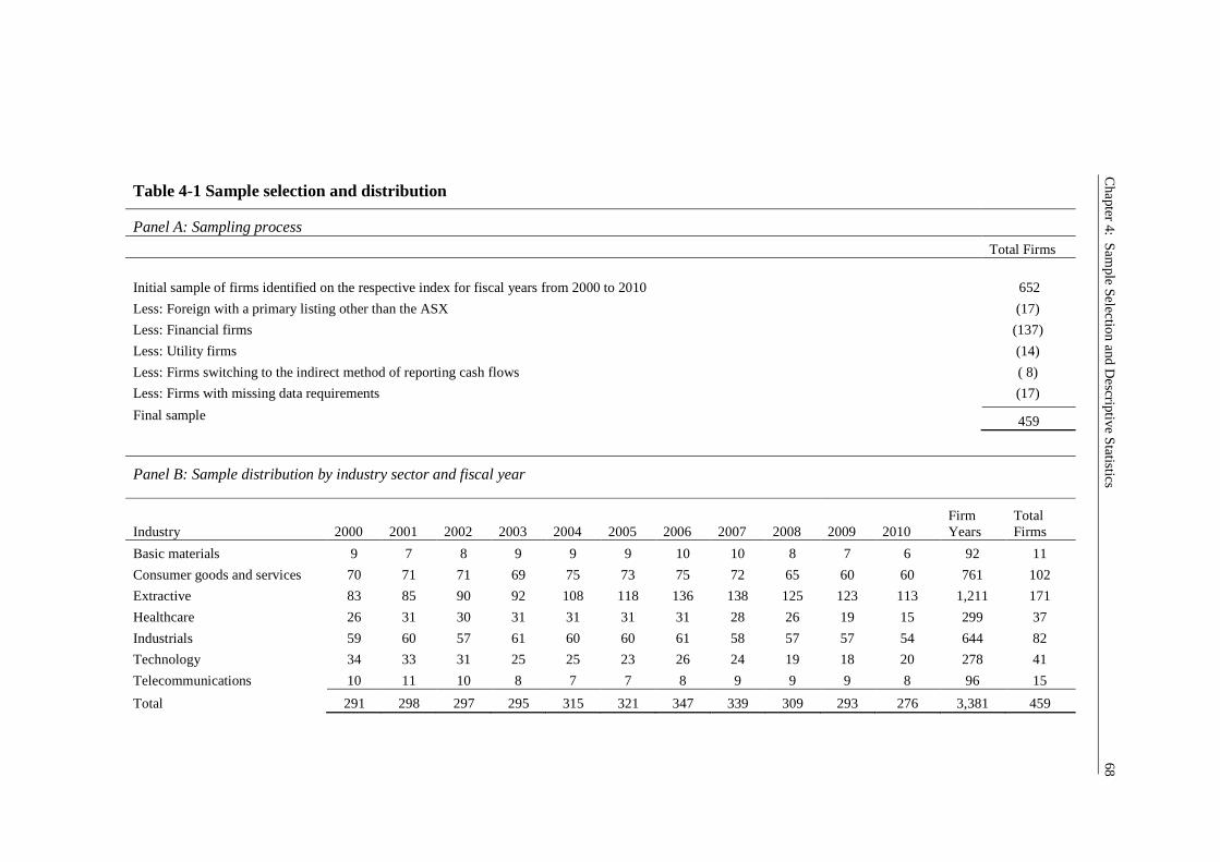
Chapter
4:S
ample
Selectio
nand
Descriptive
Statistics
68
Table 4-1 Sample selection and distribution
Panel A: Sampling process
Total Firms
Initial sample of firms identified on the respective index for fiscal years from 2000 to 2010 652
Less: Foreign with a primary listing other than the ASX (17)
Less: Financial firms (137)
Less: Utility firms (14)
Less: Firms switching to the indirect method of reporting cash flows ( 8)
Less: Firms with missing data requirements (17)
Final sample 459
Panel B: Sample distribution by industry sector and fiscal year
Industry 2000 2001 2002 2003 2004 2005 2006 2007 2008 2009 2010FirmYears
TotalFirms
Basic materials 9 7 8 9 9 9 10 10 8 7 6 92 11
Consumer goods and services 70 71 71 69 75 73 75 72 65 60 60 761 102
Extractive 83 85 90 92 108 118 136 138 125 123 113 1,211 171
Healthcare 26 31 30 31 31 31 31 28 26 19 15 299 37
Industrials 59 60 57 61 60 60 61 58 57 57 54 644 82
Technology 34 33 31 25 25 23 26 24 19 18 20 278 41
Telecommunications 10 11 10 8 7 7 8 9 9 9 8 96 15
Total 291 298 297 295 315 321 347 339 309 293 276 3,381 459
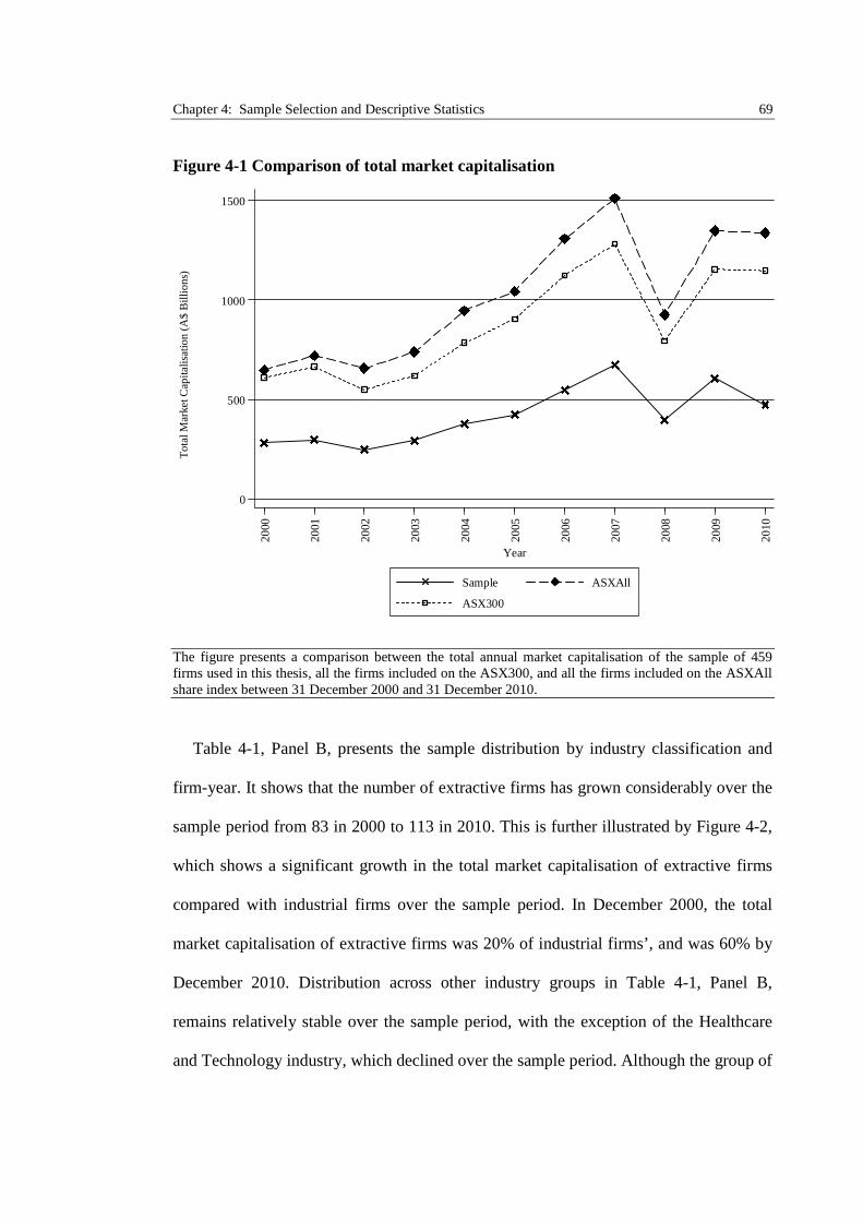
Chapter 4: Sample Selection and Descriptive Statistics 69
Figure 4-1 Comparison of total market capitalisation
The figure presents a comparison between the total annual market capitalisation of the sample of 459firms used in this thesis, all the firms included on the ASX300, and all the firms included on the ASXAllshare index between 31 December 2000 and 31 December 2010.
Table 4-1, Panel B, presents the sample distribution by industry classification and
firm-year. It shows that the number of extractive firms has grown considerably over the
sample period from 83 in 2000 to 113 in 2010. This is further illustrated by Figure 4-2,
which shows a significant growth in the total market capitalisation of extractive firms
compared with industrial firms over the sample period. In December 2000, the total
market capitalisation of extractive firms was 20% of industrial firms’, and was 60% by
December 2010. Distribution across other industry groups in Table 4-1, Panel B,
remains relatively stable over the sample period, with the exception of the Healthcare
and Technology industry, which declined over the sample period. Although the group of
0
500
1500
1000
Tot
alM
ark
etC
apit
aliz
atio
n(A
$B
illi
ons
)
2000
2001
2002
2003
2004
2005
2006
2007
2008
2009
2010
Year
Sample ASXAll
ASX300
To
tal
Mar
ket
Cap
ital
isat
ion
(A$
Bil
lio
ns)
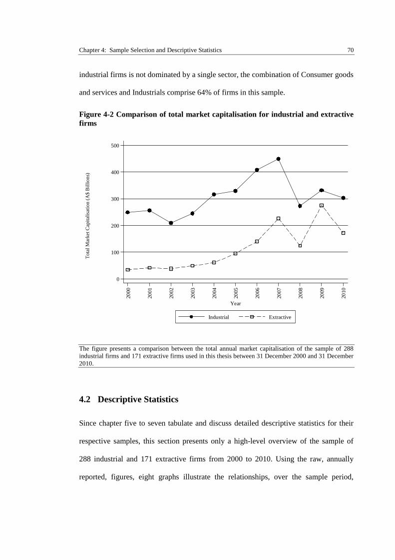
Chapter 4: Sample Selection and Descriptive Statistics 70
industrial firms is not dominated by a single sector, the combination of Consumer goods
and services and Industrials comprise 64% of firms in this sample.
Figure 4-2 Comparison of total market capitalisation for industrial and extractivefirms
The figure presents a comparison between the total annual market capitalisation of the sample of 288industrial firms and 171 extractive firms used in this thesis between 31 December 2000 and 31 December2010.
4.2 Descriptive Statistics
Since chapter five to seven tabulate and discuss detailed descriptive statistics for their
respective samples, this section presents only a high-level overview of the sample of
288 industrial and 171 extractive firms from 2000 to 2010. Using the raw, annually
reported, figures, eight graphs illustrate the relationships, over the sample period,
0
100
200
300
400
500
Tot
alM
ark
etC
apit
aliz
atio
n(A
$B
illi
ons
)
2000
2001
2002
2003
2004
2005
2006
2007
2008
2009
2010
Year
Industrial Extractive
To
tal
Mar
ket
Cap
ital
isat
ion
(A$
Bil
lio
ns)
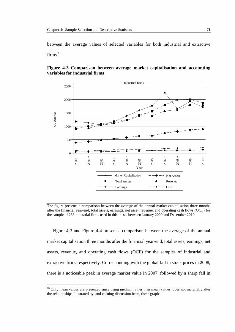
Chapter 4: Sample Selection and Descriptive Statistics 71
between the average values of selected variables for both industrial and extractive
firms.16
Figure 4-3 Comparison between average market capitalisation and accountingvariables for industrial firms
The figure presents a comparison between the average of the annual market capitalisation three monthsafter the financial year-end, total assets, earnings, net asset, revenue, and operating cash flows (OCF) forthe sample of 288 industrial firms used in this thesis between January 2000 and December 2010.
Figure 4-3 and Figure 4-4 present a comparison between the average of the annual
market capitalisation three months after the financial year-end, total assets, earnings, net
assets, revenue, and operating cash flows (OCF) for the samples of industrial and
extractive firms respectively. Corresponding with the global fall in stock prices in 2008,
there is a noticeable peak in average market value in 2007, followed by a sharp fall in
16 Only mean values are presented since using median, rather than mean values, does not materially alterthe relationships illustrated by, and ensuing discussion from, these graphs.
0
500
1000
1500
2000
2500
A$
Mil
lio
ns
2000
2001
2002
2003
2004
2005
2006
2007
2008
2009
2010
Year
Market Capitaliztion Net Assets
Total Assets Revenue
Earnings OCF
Industrial firms
Market Capitalisation
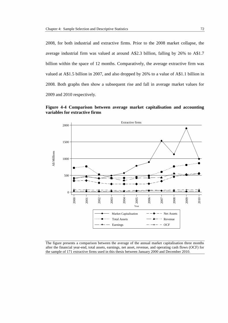
Chapter 4: Sample Selection and Descriptive Statistics 72
2008, for both industrial and extractive firms. Prior to the 2008 market collapse, the
average industrial firm was valued at around A$2.3 billion, falling by 26% to A$1.7
billion within the space of 12 months. Comparatively, the average extractive firm was
valued at A$1.5 billion in 2007, and also dropped by 26% to a value of A$1.1 billion in
2008. Both graphs then show a subsequent rise and fall in average market values for
2009 and 2010 respectively.
Figure 4-4 Comparison between average market capitalisation and accountingvariables for extractive firms
The figure presents a comparison between the average of the annual market capitalisation three monthsafter the financial year-end, total assets, earnings, net asset, revenue, and operating cash flows (OCF) forthe sample of 171 extractive firms used in this thesis between January 2000 and December 2010.
Extractive firms
0
500
1000
1500
2000
A$
Mil
lio
ns
2000
2001
2002
2003
2004
2005
2006
2007
2008
2009
2010
Year
Market Capitalization Net Assets
Total Assets Revenue
Earnings OCF
Market Capitalisation
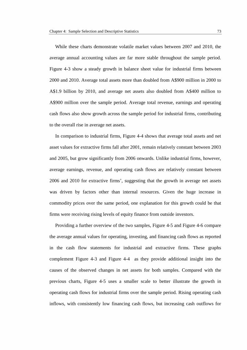
Chapter 4: Sample Selection and Descriptive Statistics 73
While these charts demonstrate volatile market values between 2007 and 2010, the
average annual accounting values are far more stable throughout the sample period.
Figure 4-3 show a steady growth in balance sheet value for industrial firms between
2000 and 2010. Average total assets more than doubled from A$900 million in 2000 to
A$1.9 billion by 2010, and average net assets also doubled from A$400 million to
A$900 million over the sample period. Average total revenue, earnings and operating
cash flows also show growth across the sample period for industrial firms, contributing
to the overall rise in average net assets.
In comparison to industrial firms, Figure 4-4 shows that average total assets and net
asset values for extractive firms fall after 2001, remain relatively constant between 2003
and 2005, but grow significantly from 2006 onwards. Unlike industrial firms, however,
average earnings, revenue, and operating cash flows are relatively constant between
2006 and 2010 for extractive firms’, suggesting that the growth in average net assets
was driven by factors other than internal resources. Given the huge increase in
commodity prices over the same period, one explanation for this growth could be that
firms were receiving rising levels of equity finance from outside investors.
Providing a further overview of the two samples, Figure 4-5 and Figure 4-6 compare
the average annual values for operating, investing, and financing cash flows as reported
in the cash flow statements for industrial and extractive firms. These graphs
complement Figure 4-3 and Figure 4-4 as they provide additional insight into the
causes of the observed changes in net assets for both samples. Compared with the
previous charts, Figure 4-5 uses a smaller scale to better illustrate the growth in
operating cash flows for industrial firms over the sample period. Rising operating cash
inflows, with consistently low financing cash flows, but increasing cash outflows for
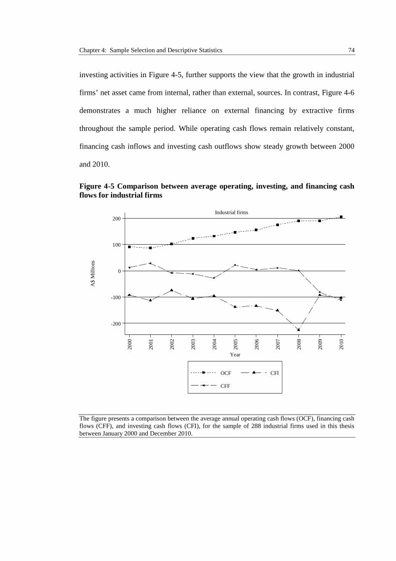
Chapter 4: Sample Selection and Descriptive Statistics 74
investing activities in Figure 4-5, further supports the view that the growth in industrial
firms’ net asset came from internal, rather than external, sources. In contrast, Figure 4-6
demonstrates a much higher reliance on external financing by extractive firms
throughout the sample period. While operating cash flows remain relatively constant,
financing cash inflows and investing cash outflows show steady growth between 2000
and 2010.
Figure 4-5 Comparison between average operating, investing, and financing cashflows for industrial firms
The figure presents a comparison between the average annual operating cash flows (OCF), financing cashflows (CFF), and investing cash flows (CFI), for the sample of 288 industrial firms used in this thesisbetween January 2000 and December 2010.
0
-200
-100
100
200
A$
Mil
lio
ns
2000
2001
2002
2003
2004
2005
2006
2007
2008
2009
2010
Year
OCF CFI
CFF
Industrial firms
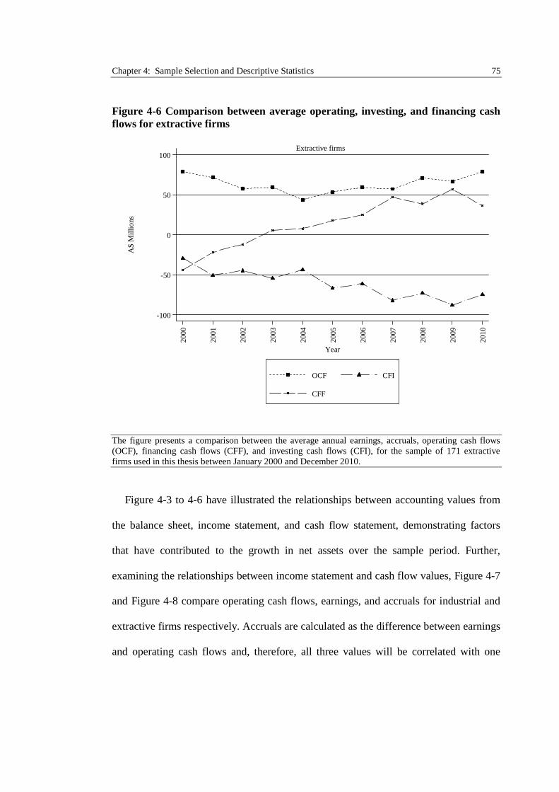
Chapter 4: Sample Selection and Descriptive Statistics 75
Figure 4-6 Comparison between average operating, investing, and financing cashflows for extractive firms
The figure presents a comparison between the average annual earnings, accruals, operating cash flows(OCF), financing cash flows (CFF), and investing cash flows (CFI), for the sample of 171 extractivefirms used in this thesis between January 2000 and December 2010.
Figure 4-3 to 4-6 have illustrated the relationships between accounting values from
the balance sheet, income statement, and cash flow statement, demonstrating factors
that have contributed to the growth in net assets over the sample period. Further,
examining the relationships between income statement and cash flow values, Figure 4-7
and Figure 4-8 compare operating cash flows, earnings, and accruals for industrial and
extractive firms respectively. Accruals are calculated as the difference between earnings
and operating cash flows and, therefore, all three values will be correlated with one
0
-100
-50
50
100
A$
Mil
lio
ns
2000
2001
2002
2003
2004
2005
2006
2007
2008
2009
2010
Year
OCF CFI
CFF
Extractive firms
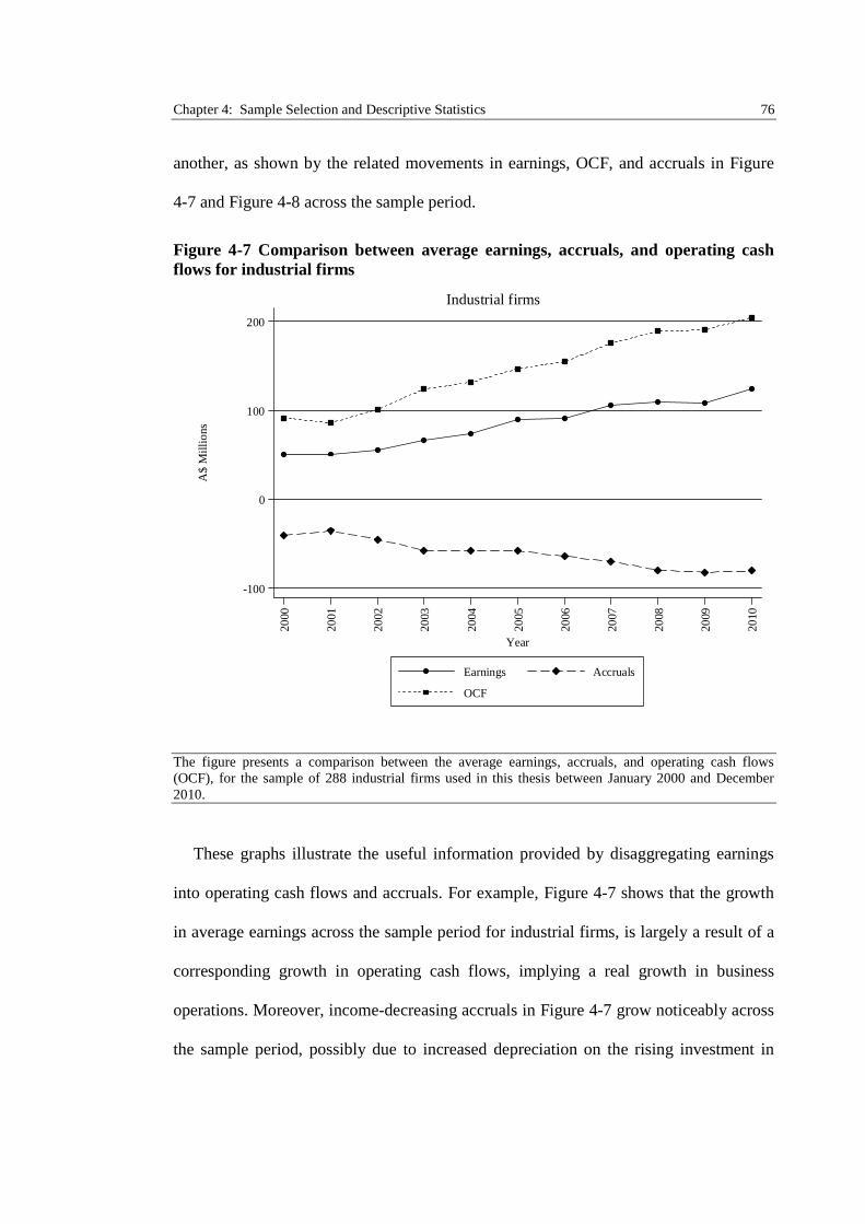
Chapter 4: Sample Selection and Descriptive Statistics 76
another, as shown by the related movements in earnings, OCF, and accruals in Figure
4-7 and Figure 4-8 across the sample period.
Figure 4-7 Comparison between average earnings, accruals, and operating cashflows for industrial firms
The figure presents a comparison between the average earnings, accruals, and operating cash flows(OCF), for the sample of 288 industrial firms used in this thesis between January 2000 and December2010.
These graphs illustrate the useful information provided by disaggregating earnings
into operating cash flows and accruals. For example, Figure 4-7 shows that the growth
in average earnings across the sample period for industrial firms, is largely a result of a
corresponding growth in operating cash flows, implying a real growth in business
operations. Moreover, income-decreasing accruals in Figure 4-7 grow noticeably across
the sample period, possibly due to increased depreciation on the rising investment in
0
-100
100
200
A$
Mil
lio
ns
2000
2001
2002
2003
2004
2005
2006
2007
2008
2009
2010
Year
Earnings Accruals
OCF
Industrial firms
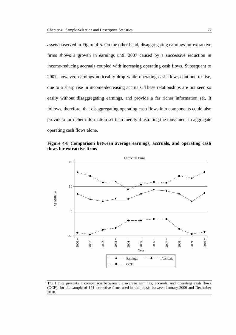
Chapter 4: Sample Selection and Descriptive Statistics 77
assets observed in Figure 4-5. On the other hand, disaggregating earnings for extractive
firms shows a growth in earnings until 2007 caused by a successive reduction in
income-reducing accruals coupled with increasing operating cash flows. Subsequent to
2007, however, earnings noticeably drop while operating cash flows continue to rise,
due to a sharp rise in income-decreasing accruals. These relationships are not seen so
easily without disaggregating earnings, and provide a far richer information set. It
follows, therefore, that disaggregating operating cash flows into components could also
provide a far richer information set than merely illustrating the movement in aggregate
operating cash flows alone.
Figure 4-8 Comparison between average earnings, accruals, and operating cashflows for extractive firms
The figure presents a comparison between the average earnings, accruals, and operating cash flows(OCF), for the sample of 171 extractive firms used in this thesis between January 2000 and December2010.
0
-50
50
100
A$
Mil
lio
ns
2000
2001
2002
2003
2004
2005
2006
2007
2008
2009
2010
Year
Earnings Accruals
OCF
Extractive firms
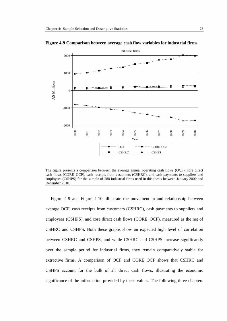
Chapter 4: Sample Selection and Descriptive Statistics 78
Figure 4-9 Comparison between average cash flow variables for industrial firms
The figure presents a comparison between the average annual operating cash flows (OCF), core directcash flows (CORE_OCF), cash receipts from customers (CSHRC), and cash payments to suppliers andemployees (CSHPS) for the sample of 288 industrial firms used in this thesis between January 2000 andDecember 2010.
Figure 4-9 and Figure 4-10, illustrate the movement in and relationship between
average OCF, cash receipts from customers (CSHRC), cash payments to suppliers and
employees (CSHPS), and core direct cash flows (CORE_OCF), measured as the net of
CSHRC and CSHPS. Both these graphs show an expected high level of correlation
between CSHRC and CSHPS, and while CSHRC and CSHPS increase significantly
over the sample period for industrial firms, they remain comparatively stable for
extractive firms. A comparison of OCF and CORE_OCF shows that CSHRC and
CSHPS account for the bulk of all direct cash flows, illustrating the economic
significance of the information provided by these values. The following three chapters
0
-2000
-1000
1000
2000A
$M
illi
on
s
2000
2001
2002
2003
2004
2005
2006
2007
2008
2009
2010
Year
OCF CORE_OCF
CSHRC CSHPS
Industrial firms
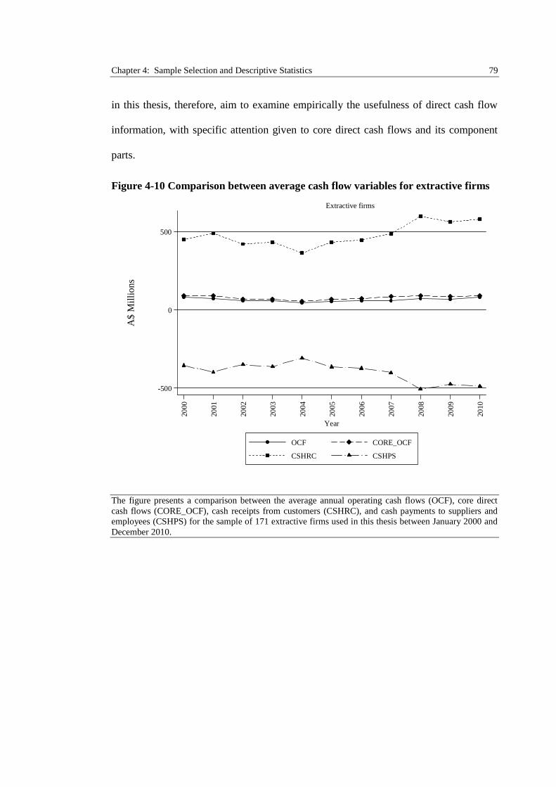
Chapter 4: Sample Selection and Descriptive Statistics 79
in this thesis, therefore, aim to examine empirically the usefulness of direct cash flow
information, with specific attention given to core direct cash flows and its component
parts.
Figure 4-10 Comparison between average cash flow variables for extractive firms
The figure presents a comparison between the average annual operating cash flows (OCF), core directcash flows (CORE_OCF), cash receipts from customers (CSHRC), and cash payments to suppliers andemployees (CSHPS) for the sample of 171 extractive firms used in this thesis between January 2000 andDecember 2010.
0
-500
500
A$
Mil
lion
s
2000
2001
2002
2003
2004
2005
2006
2007
2008
2009
2010
Year
OCF CORE_OCF
CSHRC CSHPS
Extractive firms
Chapter 5: The Value Relevance of Direct Cash Flows under IFRS 80
5The Value Relevance of Direct CashFlows under IFRS
5.1 Introduction
The International Accounting Standards Board (IASB) and Financial Accounting
Standards Board (FASB) are currently proposing that direct cash flow statements
become mandatory for all firms under their harmonised cash flow reporting
requirements.17 Prior research has shown that direct cash flow statements provide useful
information to users of financial accounts under local Generally Accepted Accounting
Principles (e.g., Jones et al., 1995; Clinch et al., 2002; Goyal, 2004). While there is
strong evidence for the usefulness of direct cash flow statements, to date, no research
has examined whether this relationship still exists under International Financial
Reporting Standards (IFRS). This chapter therefore, investigates the value relevance of
direct cash flow statements under IFRS in Australia and assesses whether there has been
a change in their value relevance since IFRS adoption.
For over 30 years, academics have strongly advocated the use of direct cash flow
statements. It is interesting to note that the promotion of this method has been driven by
a wide range of economic factors, such as liquidity problems (Ketz and Largay III,
1987), inflation and recession (Thomas, 1982), helping to provide clarity around
17 See the Proposed Accounting Standards Update FASB Staff Draft of an Exposure Draft on FinancialStatement Presentation published in July 2010 (paragraph 177).
Chapter 5: The Value Relevance of Direct Cash Flows under IFRS 81
insolvency (Trout et al., 1993).18 Throughout these times of uncertainty, direct cash
flow disclosures have been advocated to provide useful information to users of accounts.
The presentation of a direct cash flow statement allowed users of accounts to better
assess the position of the firm, despite the various economic circumstances in which
company financials were being reported.
In addition to the academic evidence on the usefulness of direct cash flow statements,
there seems to be considerable support from users of accounts. The current IASB/FASB
convergence project, if adopted, would mandate that all firms use the direct method
coupled with an indirect reconciliation as part of the financial statement notes. This
proposal received strong support in the 2009 Chartered Financial Analysis (CFA)
Institute Member Poll: Cash Flow Survey. The results indicate that of the 541
respondents, 63% either ‘agree’ or ‘strongly agree’ that the information provided in a
direct cash flow statement would help improve cash flow forecasts. Further, 94% voted
that information regarding cash receipts from customers, which is only found in direct
cash flow statements, was the most important information reported under operating cash
flows.19
Given the evidence on the usefulness of direct cash flow statements, and the demand
for the direct method from standard setters, academics and practitioners, it is important
to understand whether direct cash flow statements provide relevant information in an
IFRS reporting environment. There is a growing body of evidence that suggests
countries who have adopted IFRS experienced an overall increase in financial reporting
18 Trout et al. (1993) note how in 1987 the management of Chicago Central & Pacific Railroad Companywere able to withdraw their Chapter 11 bankruptcy filing , after presenting direct cash flow statements totheir bankers, which accurately identified the variances within the firm’s cash flow budget therebyallowing the company to secure a much needed credit facility.19 It is worth noting that some preparers of accounts are opposed to the mandating of the direct method asa result of the additional disclosure costs firms would have to incur (Hales and Orpurt, 2012).
Chapter 5: The Value Relevance of Direct Cash Flows under IFRS 82
quality, comparability, and general usefulness in the accounting information presented
to investors (Daske and Gebhardt, 2006; Barth et al., 2008). Therefore, if IFRS has
improved the financial reporting environment, it may be the case that direct cash flow
disclosures are less relevant, as a result of the better information set provided by
accounts prepared under IFRS. Consequently, the need for mandated direct cash flow
statements becomes less clear given the implied cost of disclosure. However, the move
to IFRS is likely to result in a large amount of uncertainty around any accounting
numbers that are produced in the first few years of IFRS adoption, as investors will
require time to adjust to the new accounting regime.20 Bissessur and Hodgson (2011)
for example show that post-IFRS, stock market synchronicity initially fell before
increasing significantly. However, they caveat their results, as IFRS may not have
unequivocally increased financial reporting quality in Australia, noting that an increased
reliance on industry level information may explain their results. Direct cash flow
statements may therefore become more relevant under IFRS, as historically, operating
cash flows have provided investors with a stable source of information during times of
uncertainty (Thomas, 1982).
Using a sample of non-financial companies listed on the ASX 300 from 2000-2010
this chapter examines whether there has been a change in the value relevance of direct
cash flow statements under IFRS relative to AGAAP. Australia provides an ideal
research environment to test this question, as Australia was one of the few countries to
mandate direct cash flow statements under local GAAP, and most firms still follow this
approach under IFRS, despite Australia allowing firms to choose between the direct and
20 Prior to the adoption of IFRS, Ernst and Young (2005) anticipated that remaining differences betweenAGAAP and IFRS would lead to an overall 6% increase in profits and a 15% decrease in net assets underIFRS because of the changes brought about by the new standards.
Chapter 5: The Value Relevance of Direct Cash Flows under IFRS 83
the indirect method since 2008.21 In addition, early adoption was prohibited and so
IFRS reporting only came into effect for financial years beginning on or after 1 January
2005. This distinct break point in the reporting environment, therefore, will allow for a
test of the value relevance of direct cash flow statements under IFRS. The results show
that there has been a significant increase in the value relevance of both headline
operating cash flow and in direct cash flow components for industrial firms. The
findings suggest therefore, that direct cash flow statements have increased in value
relevance under IFRS compared with AGAAP, and therefore remain a useful source of
information to users of financial accounts.
5.2 Literature Review
5.2.1 Usefulness of Reporting Direct Cash Flows
Debating the disclosure of operating cash flows has been central in the development of
all cash flow reporting standards over the past three decades. At the heart of this debate
has been whether to allow firms the choice of reporting operating cash flows either
under the indirect or direct method. Even before cash flow disclosures were
standardised, academics had begun to express their preference for the direct approach
(e.g., Paton, 1963; Heath, 1978; Lee, 1981; Thomas, 1982; Ketz and Largay III, 1987).
Moreover, after cash flow disclosure requirements became common in accounting
regimes around world, U.S. and Australian surveys conducted on diverse groups of
accounting and finance academics and professionals all indicate continuing support for
the direct approach (e.g., Jones et al., 1995; McEnroe, 1996; Smith and Freeman, 1996;
Jones and Ratnatunga, 1997; Jones and Widjaja, 1998; Goyal, 2004).
21 See Bradbury (2011) for further discussion.
Chapter 5: The Value Relevance of Direct Cash Flows under IFRS 84
Although the IASB and FASB are advocating mandating direct method cash flow
statements, few countries have previously done so,22 and critics of mandating the direct
method question whether the theoretical reporting benefits, outweigh the cost of
changing accounting systems to capture the required information.23 There is, however, a
small but growing body of evidence that shows the inclusion of estimated or actual
direct cash flow statements components increase the explanatory power and accuracy of
cash flow and earnings prediction models (e.g., Krishnan and Largay III, 2000; Arthur
and Chuang, 2008; Cheng and Hollie, 2008; Orpurt and Zang, 2009; Arthur et al., 2010;
Farshadfar and Monem, 2012, 2013). Moreover, there is also strong evidence for the
value relevance of direct cash flows (e.g., Livnat and Zarowin, 1990; Clinch et al., 2002;
Orpurt and Zang, 2009).
Livnat and Zarowin (1990) examine the value relevance of estimated direct cash
flow components and find a significant relationship between unexpected changes in
estimated direct cash flows and annual abnormal stock returns. Moreover, Clinch et al.
(2002), using actual direct cash flow statements for a sample of Australian firms, show
that direct cash flow components are value relevant and have a direct correlation in
forecasting future cash flows and annual stock returns. In addition, Orpurt and Zang
(2009) find that U.S. firms that voluntarily report direct cash flows have a higher
correlation between their stock prices and future earnings than firms using the indirect
method.
22 Australia, New Zealand and China were the only nations that have ever mandated the use of the directapproach (Wallace et al., 1997; Clinch et al., 2002).23 See the comment letters from the FASB Preliminary Views on Financial Statement PresentationReference Number: 1630-100 published in 2009.
Chapter 5: The Value Relevance of Direct Cash Flows under IFRS 85
5.2.2 Impact of Reporting Under IFRS
Investigating the impact of early adoption of IFRS, Barth et al. (2008) and Daske and
Gebhardt (2006) both find a significant improvement in financial reporting quality of
those firms that switched from local GAAP to IFRS. Notably, Barth et al. (2008) found
increased value relevance of earnings under IFRS, whilst Daske and Gebhardt (2006)
observed that users perceived IFRS financial statements to be of significantly higher
quality than those prepared under local GAAP. Although these early studies provide
some evidence for increased financial reporting quality, it was only after the 2005
mandatory adoption of IFRS by the E.U. and Australia that the impact of reporting
under IFRS could be further examined by using far larger and richer data sets.
Daske et al. (2008) provides evidence on the economic benefits of IFRS adoption,
with a general decline in cost of capital and an increase in Tobin’s Q in the pre-adoption
year, followed by an increase in capital market liquidity post-adoption. However,
increased market liquidity under IFRS only occurred in countries with strong reporting
incentives and legal enforcement of the standards. This result is consistent with the
views of Ball (2006) and Soderstrom and Sun (2007), who postulated that the perceived
benefits associated with the global mandatory adoption of IFRS, would be dependent
upon the effectiveness of the enforcement of IFRS. Byard et al.’s (2011) findings
further emphasise the important role of effective enforcement, as their results show a
significant decline in analyst forecast errors following the mandatory adoption of IFRS
in Europe, but only for firms in countries with a strong legal environment.
Chapter 5: The Value Relevance of Direct Cash Flows under IFRS 86
5.2.3 Adoption of IFRS by Australia
Australia provides an ideal setting in which to examine the impact of reporting under
IFRS since there is a regime of high quality accounting enforcement coupled with low
manipulation incentives (Bissessur and Hodgson, 2011; Cotter et al., 2012). Moreover,
unlike the E.U., Australia prohibited the early adoption of IFRS. Consequently, any
empirical results on the impact of IFRS adoption are free from early adoption bias. The
Australian government had been on a process of IFRS convergence since 1996 (Tarca,
2004). However, by the time firms adopted the Australian equivalents of IFRS there
were still noteworthy differences between the two standards.24 If these differences were
not significant then the mandatory adoption of IFRS would have caused very little or no
change at all in the value relevance of accounting information (Aharony et al., 2010). In
fact recent studies specifically examining Australian firms have found that there has
been a significant change in the value relevance of accounting information subsequent
to adopting IFRS, evidenced by an increased accuracy of analysts’ earnings forecasts
(Bissessur and Hodgson, 2011; Cotter et al., 2012), and an increased level of stock
market synchronicity (Bissessur and Hodgson, 2011).
5.3 Hypotheses Development
Cotter et al. (2012) and Bissessur and Hodgson (2011) both attribute their findings to a
post-IFRS improvement in accounting information. However, an important question
24 Some of the more significant differences between Australian GAAP and IFRS include IFRSprohibiting the disclosure of extraordinary items; disallowing the use of the full liability method ofaccounting for deferred taxation; prohibiting the recognition of certain non-goodwill related internallygenerated intangible assets; accounting for changes in the fair value of investment properties through theincome statement rather than the statement of changes in equity; providing far more comprehensiverequirements and guidance for the recognition and disclosure of financial instruments; requiring therecognition and disclosure of all share based payments irrespective of whether they were applicable todirectors, executives or all staff. (Deloitte, Differences between current Australian GAAP and Australianequivalents to IFRS, published in August 2004).
Chapter 5: The Value Relevance of Direct Cash Flows under IFRS 87
that extant literature has generally left unanswered, is what specific accounting
information under IFRS has improved the quality of accounting information and
resulted in an overall improvement in earnings forecasts. Prior to the adoption of IFRS,
Ernst and Young (2005) anticipated that the remaining differences between AGAAP
and IFRS would lead to an overall 6% increase in profits, and a 15% decrease in net
assets because of the changes brought about by the new standards. The most significant
change under IFRS was the abolition of capitalising certain internally generated
intangible assets, and the introduction of assessing goodwill for annual impairment,
rather than amortising goodwill. Prior to IFRS, Matolcsy and Wyatt (2006) found a
significant positive/(negative) association between firms which capitalised intangible
assets and analyst following/(forecast errors). Further, subsequent to Australia’s
adoption of IFRS, Chalmers et al. (2010) present evidence of significantly higher
analyst forecast errors for firms reporting lower levels of internally generated
capitalised intangible assets. Taken together, these findings imply that the IASB’s
changes to intangibles in Australia may have resulted in a loss of value relevant
information.
IFRS is also thought to increase earnings volatility because of the application of fair
value accounting. Although Ball (2006) notes that increased earnings volatility is not
necessarily a problem, it becomes a problem when it is caused by ‘estimation noise’ or
‘management manipulation’. Earnings volatility may therefore be an issue under IFRS
given the increased reliance on managerial discretion that fair value measurement
requires. Moreover, as Ball (2006) notes, the recognition of both future gains and losses
in the current reporting period is one of the most significant problems associated with
Chapter 5: The Value Relevance of Direct Cash Flows under IFRS 88
fair value accounting, and this approach is contrary to the conservative accounting
approach of deferring expected future profits until realised.
Although IFRS was adopted in 2005, there were no major differences in cash flow
reporting between AASB 1026, and the IFRS equivalent to IAS 7, AASB 107 Statement
of Cash flows. Australian cash flow disclosure requirements have therefore remained
consistent under both AGAAP and IFRS, while the reporting of net assets and earnings
has changed. Cash flow reporting requirements were originally issued in order to
provide additional information amid times of growing financial instability, when
information from the balance sheet and income statement alone were not sufficient to
provide information to users of accounts (Thomas, 1982). As a result, if the changes
brought about by IFRS adoption, leads to increased uncertainty around the accounting
numbers produced under IFRS in the short run, then cash flow information, which is
reported consistently under AGAAP and IFRS, should increase in value relevance. The
first hypothesis is therefore,
H1: Value relevance of operating cash flows increases under IFRS
In addition, since AASB 107 mandated that all firms use the direct method of
reporting cash flows until 2007, operating cash flows are then disaggregated to examine
the value relevance of direct cash flow components under IFRS. Further, both ‘core’
and ‘non-core’ direct cash flow disclosures are then analysed, given the perceived
benefits of direct cash flow statements as a source of useful information for users of
accounts, and the belief by analysts that components such as cash receipts from
customers are useful informational disclosures. Prior research has shown that ‘core’
direct cash flows have been found to be more useful in forecasting future cash flows
Chapter 5: The Value Relevance of Direct Cash Flows under IFRS 89
than either ‘non-core’ or aggregate operating cash flows alone (Cheng and Hollie,
2008).25
In a 2009 CFA survey, the majority of respondents agreed that information provided
by direct cash flow statements would improve their cash flow forecasts. Specifically, of
those who responded, the direct cash flow component of ‘cash receipts from customers’
was considered to be the most important information within the operating section of a
direct cash flow statement. Prior research has shown an increase in power and accuracy
of cash flow and earnings prediction models after including direct cash flow
components (e.g., Krishnan and Largay III, 2000; Arthur and Chuang, 2008; Cheng and
Hollie, 2008; Orpurt and Zang, 2009; Arthur et al., 2010). Further, studies also provide
strong evidence of the value relevance of direct cash flows (e.g., Livnat and Zarowin,
1990; Clinch et al., 2002; Orpurt and Zang, 2009). Accordingly, a rise in the value
relevance of ‘core’ direct cash flows and direct cash flow components under IFRS is
predicted. The second hypothesis is therefore,
H2: The value relevance of core direct cash flows and direct cash flow components
increases under IFRS
5.4 Model Development and Data
5.4.1 Model Construction
Price levels models are often used to provide standard setters with insights into the
value relevance of specific accounting information (Barth et al., 2001a). To examine the
25 ‘Core’ direct cash flows are calculated as the net amount of cash receipts from customers and cashpayments to suppliers and employees. ‘Non-core’ direct cash flows include all other operating cash flows.Cheng and Hollie (2008) find that ‘core’ cash flows showed a higher level of persistence into future cashflows than ‘non-core’ cash flows. Moreover, this model revealed a higher explanatory power whencompared with the more parsimonious model using aggregate operating cash flows.
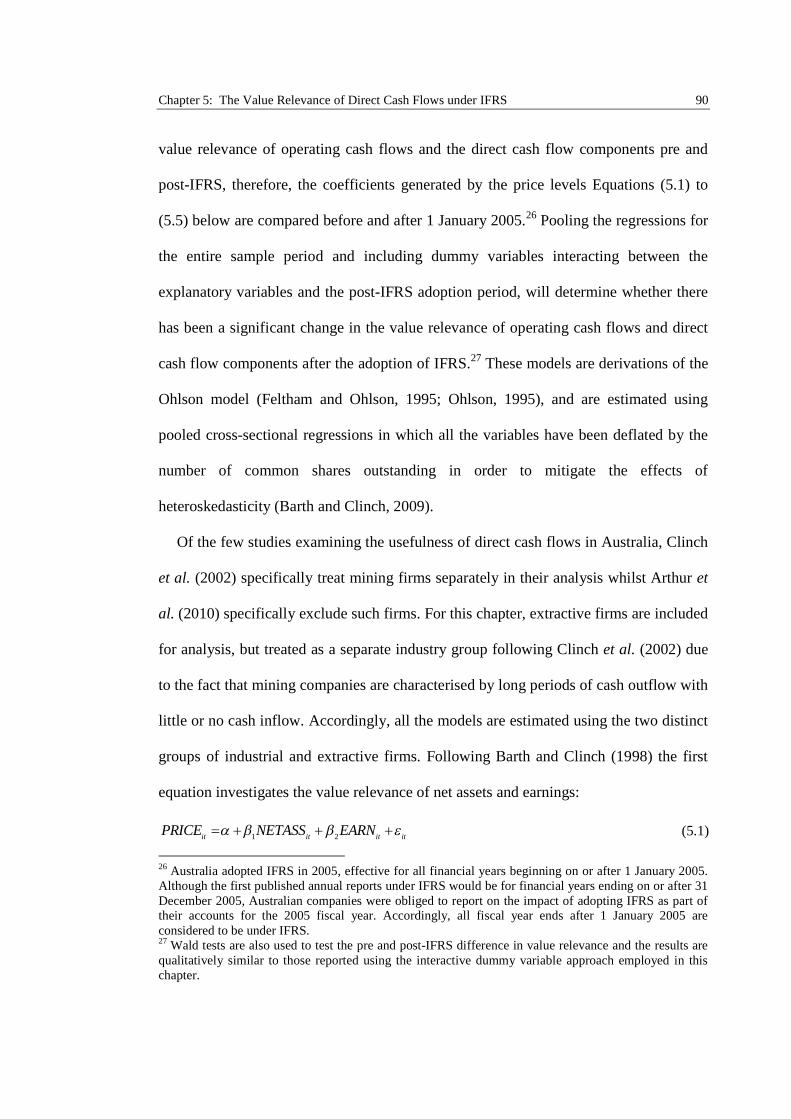
Chapter 5: The Value Relevance of Direct Cash Flows under IFRS 90
value relevance of operating cash flows and the direct cash flow components pre and
post-IFRS, therefore, the coefficients generated by the price levels Equations (5.1) to
(5.5) below are compared before and after 1 January 2005.26 Pooling the regressions for
the entire sample period and including dummy variables interacting between the
explanatory variables and the post-IFRS adoption period, will determine whether there
has been a significant change in the value relevance of operating cash flows and direct
cash flow components after the adoption of IFRS.27 These models are derivations of the
Ohlson model (Feltham and Ohlson, 1995; Ohlson, 1995), and are estimated using
pooled cross-sectional regressions in which all the variables have been deflated by the
number of common shares outstanding in order to mitigate the effects of
heteroskedasticity (Barth and Clinch, 2009).
Of the few studies examining the usefulness of direct cash flows in Australia, Clinch
et al. (2002) specifically treat mining firms separately in their analysis whilst Arthur et
al. (2010) specifically exclude such firms. For this chapter, extractive firms are included
for analysis, but treated as a separate industry group following Clinch et al. (2002) due
to the fact that mining companies are characterised by long periods of cash outflow with
little or no cash inflow. Accordingly, all the models are estimated using the two distinct
groups of industrial and extractive firms. Following Barth and Clinch (1998) the first
equation investigates the value relevance of net assets and earnings:
1 2
it it it itPRICE NETASS EARN (5.1)
26 Australia adopted IFRS in 2005, effective for all financial years beginning on or after 1 January 2005.Although the first published annual reports under IFRS would be for financial years ending on or after 31December 2005, Australian companies were obliged to report on the impact of adopting IFRS as part oftheir accounts for the 2005 fiscal year. Accordingly, all fiscal year ends after 1 January 2005 areconsidered to be under IFRS.27 Wald tests are also used to test the pre and post-IFRS difference in value relevance and the results arequalitatively similar to those reported using the interactive dummy variable approach employed in thischapter.
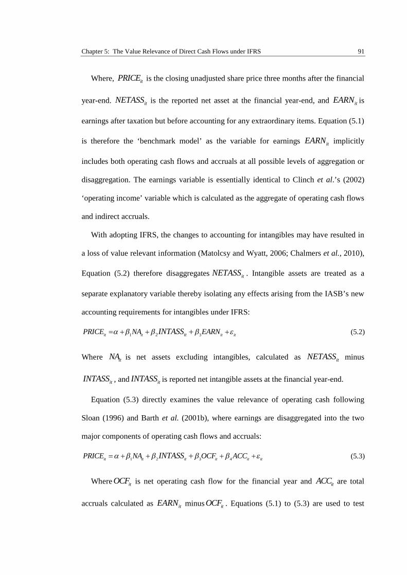
Chapter 5: The Value Relevance of Direct Cash Flows under IFRS 91
Where, itPRICE is the closing unadjusted share price three months after the financial
year-end. itNETASS is the reported net asset at the financial year-end, and itEARN is
earnings after taxation but before accounting for any extraordinary items. Equation (5.1)
is therefore the ‘benchmark model’ as the variable for earnings itEARN implicitly
includes both operating cash flows and accruals at all possible levels of aggregation or
disaggregation. The earnings variable is essentially identical to Clinch et al.’s (2002)
‘operating income’ variable which is calculated as the aggregate of operating cash flows
and indirect accruals.
With adopting IFRS, the changes to accounting for intangibles may have resulted in
a loss of value relevant information (Matolcsy and Wyatt, 2006; Chalmers et al., 2010),
Equation (5.2) therefore disaggregates itNETASS . Intangible assets are treated as a
separate explanatory variable thereby isolating any effects arising from the IASB’s new
accounting requirements for intangibles under IFRS:
1 32 it it it ititPRICE NA EARNINTASS (5.2)
Where itNA is net assets excluding intangibles, calculated as itNETASS minus
itINTASS , and itINTASS is reported net intangible assets at the financial year-end.
Equation (5.3) directly examines the value relevance of operating cash following
Sloan (1996) and Barth et al. (2001b), where earnings are disaggregated into the two
major components of operating cash flows and accruals:
21 3 4
it it it it it itPRICE NA OCF ACCINTASS (5.3)
Where itOCF is net operating cash flow for the financial year and itACC are total
accruals calculated as itEARN minus itOCF . Equations (5.1) to (5.3) are used to test
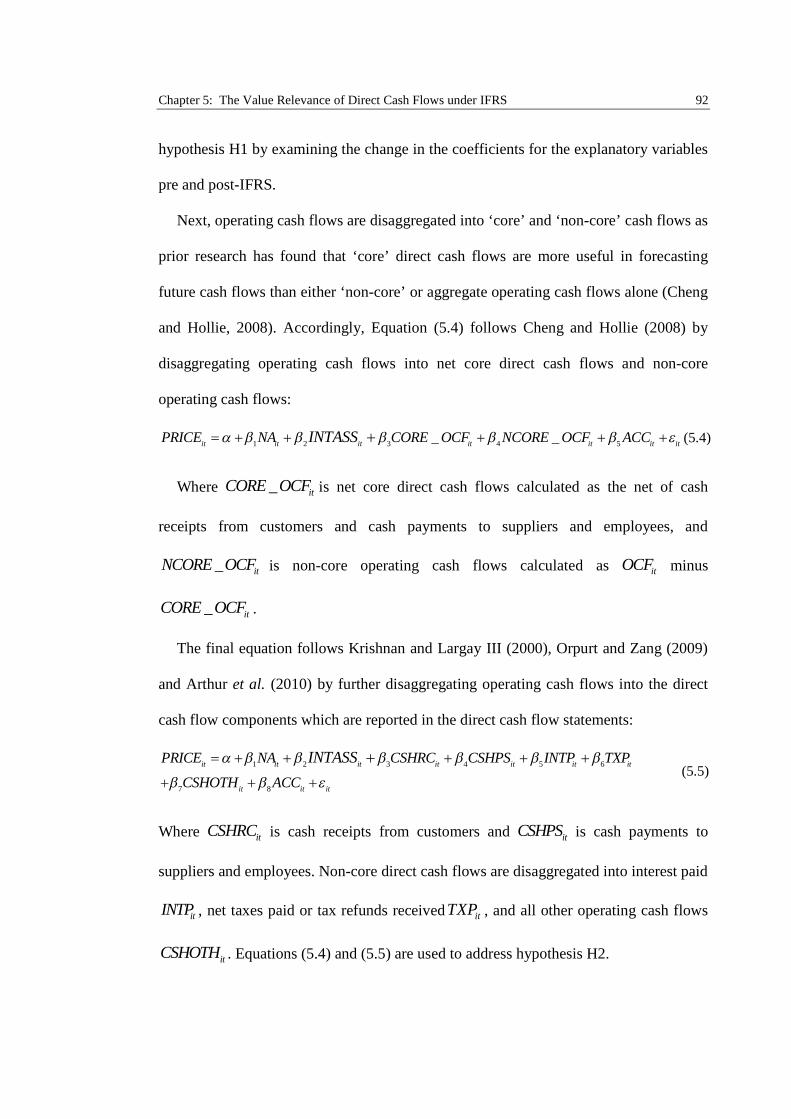
Chapter 5: The Value Relevance of Direct Cash Flows under IFRS 92
hypothesis H1 by examining the change in the coefficients for the explanatory variables
pre and post-IFRS.
Next, operating cash flows are disaggregated into ‘core’ and ‘non-core’ cash flows as
prior research has found that ‘core’ direct cash flows are more useful in forecasting
future cash flows than either ‘non-core’ or aggregate operating cash flows alone (Cheng
and Hollie, 2008). Accordingly, Equation (5.4) follows Cheng and Hollie (2008) by
disaggregating operating cash flows into net core direct cash flows and non-core
operating cash flows:
2 31 4 5 _ _
it it it it it it itPRICE NA CORE OCF NCORE OCF ACCINTASS (5.4)
Where _ itCORE OCF is net core direct cash flows calculated as the net of cash
receipts from customers and cash payments to suppliers and employees, and
_ itNCORE OCF is non-core operating cash flows calculated as itOCF minus
_ itCORE OCF .
The final equation follows Krishnan and Largay III (2000), Orpurt and Zang (2009)
and Arthur et al. (2010) by further disaggregating operating cash flows into the direct
cash flow components which are reported in the direct cash flow statements:
2 3 4 5 6
7
1
8
it it it it it it it
it it it
PRICE NA CSHRC CSHPS INTP TXP
CSHOTH ACC
INTASS
(5.5)
Where itCSHRC is cash receipts from customers and itCSHPS is cash payments to
suppliers and employees. Non-core direct cash flows are disaggregated into interest paid
itINTP , net taxes paid or tax refunds received itTXP , and all other operating cash flows
itCSHOTH . Equations (5.4) and (5.5) are used to address hypothesis H2.
Chapter 5: The Value Relevance of Direct Cash Flows under IFRS 93
5.4.2 Sample Construction and Descriptive Statistics
The initial sample consists of 652 firms representing companies listed on the Australian
Stock Exchange (ASX) 300 index at the end of each of the ten years from 2000-2010.28
From this list, financials and utilities firms are removed, along with firms that are not
primarily listed on the ASX, and firms missing key financial information.29 All firms
that subsequently chose to report their cash flows under the indirect method are also
removed.30 Only eight firms in the sample chose to switch from the direct to the indirect
method. The low uptake of the indirect method by Australian companies is likely a
result of Australian firms having already invested in the information systems needed to
capture the requisite information reported in a direct cash flow statement (Bond et al.,
2012). Accordingly, there is no added cost for Australian firms to continue reporting
direct cash flows since this is effectively a sunk cost. In addition, the removal of this
information may be viewed as a negative signal as the firm would be disclosing less
information than previously, and so firms are not willing to switch. Consequently, if
firms are disclosing direct cash flow components, they are likely to continue doing so,
even when given the option to switch.
The final sample of 459 firms shown in Table 5-1, Panel A, represents, on average,
one third of market capitalisation of all domestic firms listed on the ASX throughout the
sample period. This specifically includes mining and natural resources exploration
companies. However, in line with Clinch et al. (2002), mining and natural resources
28 The ASX300 comprises the 300 largest firms in Australia.29 Financial firms are removed because of their different reporting requirements and utility firms areexcluded given their oligopolistic status. Foreign domiciled firms are also excluded from the sample, asthey do not follow Australian GAAP.30 Australian firms were first permitted a choice between reporting their operating cash flows using thedirect or indirect method when in April 2007 the AASB amended AASB 107 by issuing AASBAmendment Pronouncement (AP) 2007-4 thereby allowing firms with the alternative option. The mainpurpose of issuing AASB 2007-4 was to include all options available under IFRS in the Australianequivalents to IFRS in order to eliminate the remaining differences between the different standards.
Chapter 5: The Value Relevance of Direct Cash Flows under IFRS 94
exploration companies are treated as a unique group of ‘extractive’ firms, whilst all
remaining firms are classified as a further sample of ‘industrial’ firms. All financial data
is obtained from the Aspect Huntley database, which provides a detailed breakdown of
the direct cash flow components that are otherwise unavailable elsewhere.
Table 5-1, Panel B, presents the sample distribution by industry classification and
firm-year. It reveals that the number of extractive firms has grown considerably over the
sample period from 83 in 2000 to 113 in 2010. The distribution across other industry
groups remains relatively stable over the sample period, with the exception of the
Healthcare and Technology industry, which sees a sharp fall in numbers by the end of
2010. Although the group of industrial firms is not dominated by a single sector,
Consumer goods and services and Industrials combined comprise 64% of firms in this
sample.
Summary descriptive statistics reported in Table 5-1, Panel C, presents the market
capitalisation, net assets, total assets, earnings, operating cash flows and revenue of the
pooled sample of industrial firms and extractive firms as well as the pre and post-IFRS
periods. Consistent with Clinch et al. (2002), this table shows that all the variables are
highly positively skewed for both industrial and extractive firms. Further, the means and
medians for the variables in the industrial sample are consistently larger than extractive
firms. Although the means and medians for most of the variables for extractive firms
are roughly half the size of industrial firms, the medians for earnings, operating cash
flows and revenue of extractive firms are all less than 10% of those for industrial
Chapter 5: The Value Relevance of Direct Cash Flows under IFRS 95
firms.31 This is most likely due to the nature of the industry, which requires a lengthy
start-up period of exploration before revenue generation begins. Finally, means and
medians of all variables are shown to increase noticeably after the adoption of IFRS,
with the exception of median earnings, operating cash flow and revenue for extractive
firms.
Table 5-2 provides summary descriptive statistics of all the variables used in the
regression analysis, which are standardised by common shares outstanding at the
financial year-end to mitigate any potential scale effects (Barth and Clinch, 2009).
Consistent with the unscaled variables in Table 5-1, Panel C, the deflated variables in
Table 5-2 Panel A are positively skewed with average share price, net assets, earnings
and operating cash flows per share being larger for industrial than extractive firms.
Further, the mean value per share of each variable increases in the post-IFRS period.
Overall, the summary statistics in Table 5-2, Panel A are in line with those in Clinch et
al. (2002).
31 The comparatively smaller size of the variables for extractive firms is partly due to the exclusion of RioTinto and BHP Billiton, two of the largest extractive firms. These firms are excluded because of thesample selection criteria to exclude all firms reporting indirect cash flow statements during the sampleperiod. Rio Tinto Limited and Rio Tinto Plc. merged in December 1995, subsequent to which the groupreported under U.K. GAAP using the indirect method of cash flow reporting. BHP Billiton elected toreport their cash flow statement using the indirect method from 2008 after the AASB provided firms witha choice between the two methods. As a result, both for these firms were dropped from the analysis.

Chapter
5:T
heV
alueR
elevanceof
Direct
Cash
Flo
ws
und
erIF
RS
96
Table 5-1 Sample selection and distribution
Panel A: Sampling process
Total Firms
Initial sample of firms identified on the respective index for fiscal years from 2000 to 2009 652
Less: Foreign with a primary listing other than the ASX (17)
Less: Financial firms (137)
Less: Utility firms (14)
Less: Firms switching to the indirect method of reporting cash flows ( 8)
Less: Firms with missing data requirements (17)
Final sample 459
Panel B: Sample distribution by industry sector and fiscal year
Industry 2000 2001 2002 2003 2004 2005 2006 2007 2008 2009 2010FirmYears
TotalFirms
Basic materials 9 7 8 9 9 9 10 10 8 7 6 92 11
Consumer goods and services 70 71 71 69 75 73 75 72 65 60 60 761 102
Extractive 83 85 90 92 108 118 136 138 125 123 113 1,211 171
Healthcare 26 31 30 31 31 31 31 28 26 19 15 299 37
Industrials 59 60 57 61 60 60 61 58 57 57 54 644 82
Technology 34 33 31 25 25 23 26 24 19 18 20 278 41
Telecommunications 10 11 10 8 7 7 8 9 9 9 8 96 15
Total 291 298 297 295 315 321 347 339 309 293 276 3,381 459
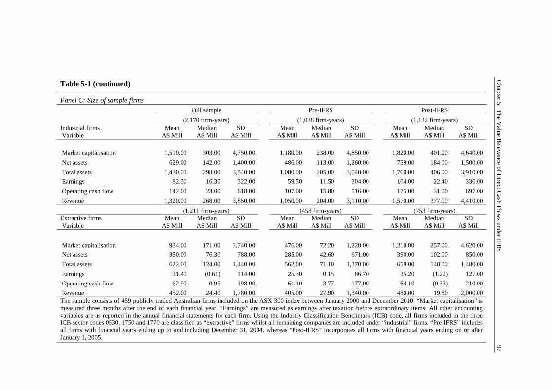
Chapter
5:T
heV
alueR
elevanceof
Direct
Cash
Flo
ws
und
erIF
RS
97
Table 5-1 (continued)
Panel C: Size of sample firms
Full sample Pre-IFRS Post-IFRS
(2,170 firm-years) (1,038 firm-years) (1,132 firm-years)Industrial firms Mean Median SD Mean Median SD Mean Median SDVariable A$ Mill A$ Mill A$ Mill A$ Mill A$ Mill A$ Mill A$ Mill A$ Mill A$ Mill
Market capitalisation 1,510.00 303.00 4,750.00 1,180.00 238.00 4,850.00 1,820.00 401.00 4,640.00
Net assets 629.00 142.00 1,400.00 486.00 113.00 1,260.00 759.00 184.00 1,500.00
Total assets 1,430.00 298.00 3,540.00 1,080.00 205.00 3,040.00 1,760.00 406.00 3,910.00
Earnings 82.50 16.30 322.00 59.50 11.50 304.00 104.00 22.40 336.00
Operating cash flow 142.00 23.00 618.00 107.00 15.80 516.00 175.00 31.00 697.00
Revenue 1,320.00 268.00 3,850.00 1,050.00 204.00 3,110.00 1,570.00 377.00 4,410.00
(1,211 firm-years) (458 firm-years) (753 firm-years)Extractive firms Mean Median SD Mean Median SD Mean Median SDVariable A$ Mill A$ Mill A$ Mill A$ Mill A$ Mill A$ Mill A$ Mill A$ Mill A$ Mill
Market capitalisation 934.00 171.00 3,740.00 476.00 72.20 1,220.00 1,210.00 257.00 4,620.00
Net assets 350.00 76.30 788.00 285.00 42.60 671.00 390.00 102.00 850.00
Total assets 622.00 124.00 1,440.00 562.00 71.10 1,370.00 659.00 148.00 1,480.00
Earnings 31.40 (0.61) 114.00 25.30 0.15 86.70 35.20 (1.22) 127.00
Operating cash flow 62.90 0.95 198.00 61.10 3.77 177.00 64.10 (0.33) 210.00
Revenue 452.00 24.40 1,780.00 405.00 27.90 1,340.00 480.00 19.80 2,000.00The sample consists of 459 publicly traded Australian firms included on the ASX 300 index between January 2000 and December 2010. “Market capitalisation” ismeasured three months after the end of each financial year. “Earnings” are measured as earnings after taxation before extraordinary items. All other accountingvariables are as reported in the annual financial statements for each firm. Using the Industry Classification Benchmark (ICB) code, all firms included in the threeICB sector codes 0530, 1750 and 1770 are classified as “extractive” firms whilst all remaining companies are included under “industrial” firms. “Pre-IFRS” includesall firms with financial years ending up to and including December 31, 2004, whereas “Post-IFRS” incorporates all firms with financial years ending on or afterJanuary 1, 2005.
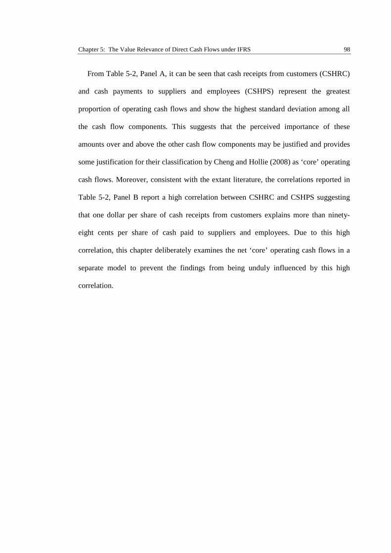
Chapter 5: The Value Relevance of Direct Cash Flows under IFRS 98
From Table 5-2, Panel A, it can be seen that cash receipts from customers (CSHRC)
and cash payments to suppliers and employees (CSHPS) represent the greatest
proportion of operating cash flows and show the highest standard deviation among all
the cash flow components. This suggests that the perceived importance of these
amounts over and above the other cash flow components may be justified and provides
some justification for their classification by Cheng and Hollie (2008) as ‘core’ operating
cash flows. Moreover, consistent with the extant literature, the correlations reported in
Table 5-2, Panel B report a high correlation between CSHRC and CSHPS suggesting
that one dollar per share of cash receipts from customers explains more than ninety-
eight cents per share of cash paid to suppliers and employees. Due to this high
correlation, this chapter deliberately examines the net ‘core’ operating cash flows in a
separate model to prevent the findings from being unduly influenced by this high
correlation.
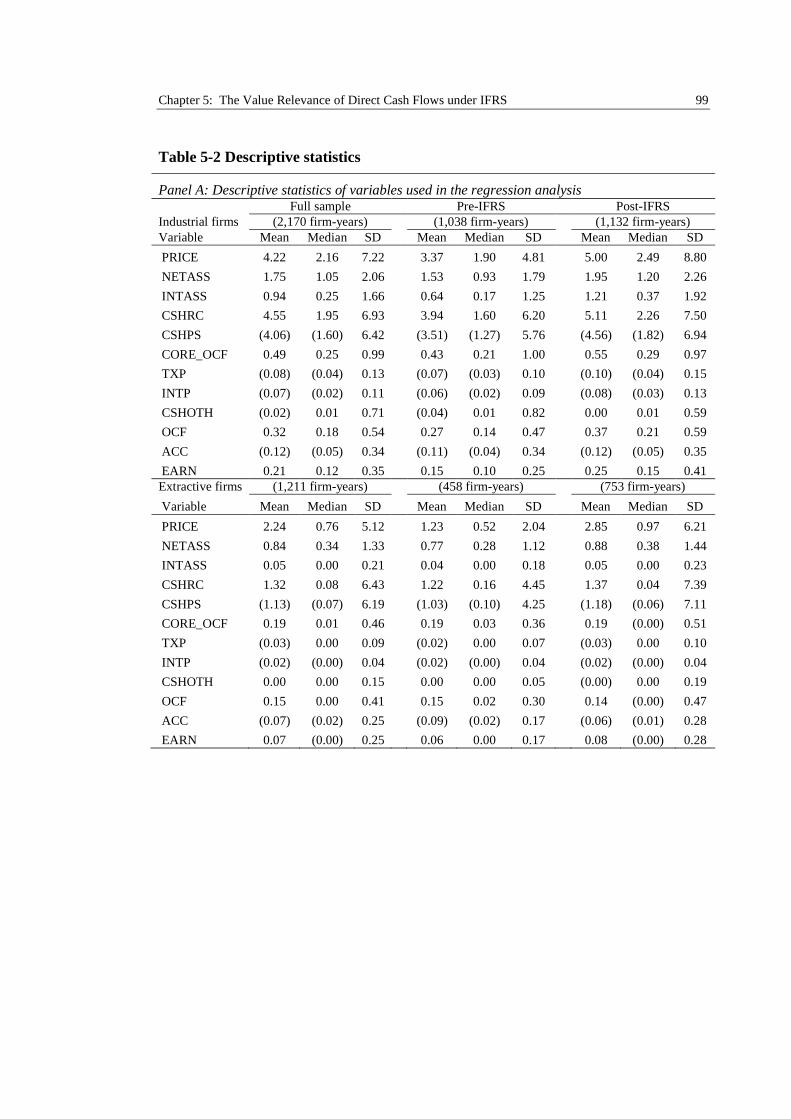
Chapter 5: The Value Relevance of Direct Cash Flows under IFRS 99
Table 5-2 Descriptive statistics
Panel A: Descriptive statistics of variables used in the regression analysisFull sample Pre-IFRS Post-IFRS
Industrial firms (2,170 firm-years) (1,038 firm-years) (1,132 firm-years)Variable Mean Median SD Mean Median SD Mean Median SD
PRICE 4.22 2.16 7.22 3.37 1.90 4.81 5.00 2.49 8.80
NETASS 1.75 1.05 2.06 1.53 0.93 1.79 1.95 1.20 2.26
INTASS 0.94 0.25 1.66 0.64 0.17 1.25 1.21 0.37 1.92
CSHRC 4.55 1.95 6.93 3.94 1.60 6.20 5.11 2.26 7.50
CSHPS (4.06) (1.60) 6.42 (3.51) (1.27) 5.76 (4.56) (1.82) 6.94
CORE_OCF 0.49 0.25 0.99 0.43 0.21 1.00 0.55 0.29 0.97
TXP (0.08) (0.04) 0.13 (0.07) (0.03) 0.10 (0.10) (0.04) 0.15
INTP (0.07) (0.02) 0.11 (0.06) (0.02) 0.09 (0.08) (0.03) 0.13
CSHOTH (0.02) 0.01 0.71 (0.04) 0.01 0.82 0.00 0.01 0.59
OCF 0.32 0.18 0.54 0.27 0.14 0.47 0.37 0.21 0.59
ACC (0.12) (0.05) 0.34 (0.11) (0.04) 0.34 (0.12) (0.05) 0.35
EARN 0.21 0.12 0.35 0.15 0.10 0.25 0.25 0.15 0.41Extractive firms (1,211 firm-years) (458 firm-years) (753 firm-years)
Variable Mean Median SD Mean Median SD Mean Median SD
PRICE 2.24 0.76 5.12 1.23 0.52 2.04 2.85 0.97 6.21
NETASS 0.84 0.34 1.33 0.77 0.28 1.12 0.88 0.38 1.44
INTASS 0.05 0.00 0.21 0.04 0.00 0.18 0.05 0.00 0.23
CSHRC 1.32 0.08 6.43 1.22 0.16 4.45 1.37 0.04 7.39
CSHPS (1.13) (0.07) 6.19 (1.03) (0.10) 4.25 (1.18) (0.06) 7.11
CORE_OCF 0.19 0.01 0.46 0.19 0.03 0.36 0.19 (0.00) 0.51
TXP (0.03) 0.00 0.09 (0.02) 0.00 0.07 (0.03) 0.00 0.10
INTP (0.02) (0.00) 0.04 (0.02) (0.00) 0.04 (0.02) (0.00) 0.04
CSHOTH 0.00 0.00 0.15 0.00 0.00 0.05 (0.00) 0.00 0.19
OCF 0.15 0.00 0.41 0.15 0.02 0.30 0.14 (0.00) 0.47
ACC (0.07) (0.02) 0.25 (0.09) (0.02) 0.17 (0.06) (0.01) 0.28
EARN 0.07 (0.00) 0.25 0.06 0.00 0.17 0.08 (0.00) 0.28
Chapter
5:T
heV
alueR
elevanceof
Direct
Cash
Flo
ws
und
erIF
RS
100
Table 5-2 (continued)
Panel B: Industrial firms (below the diagonal) and Extractive firms (above the diagonal) Pearson correlations of variables used in the regressionanalysis
Variable PRICE NETASS INTASS CSHRC CSHPS CSHRAP TXP INTP CSHOTH OCF ACC EARN
PRICE 0.506 0.087 0.249 -0.225 0.465 -0.355 -0.361 -0.189 0.329 -0.099 0.449
NETASS 0.629 0.282 0.641 -0.606 0.814 -0.640 -0.630 0.042‡ 0.708 -0.462 0.713
INTASS 0.413 0.667 0.193 -0.186 0.187 -0.174 -0.250 0.033‡ 0.154 -0.062 0.194
CSHRC 0.540 0.669 0.375 -0.998 0.569 -0.567 -0.540 0.032‡ 0.459 -0.269 0.493
CSHPS -0.500 -0.646 -0.347 -0.992 -0.518 0.535 0.520 -0.030‡ -0.410 0.234 -0.448
CSHRAP 0.541 0.496 0.370 0.568 -0.459 -0.730 -0.562 0.049‡ 0.904 -0.620 0.881
TXP -0.740 -0.644 -0.440 -0.674 0.635 -0.598 0.375 -0.047‡ -0.561 0.282 -0.651
INTP -0.392 -0.670 -0.489 -0.545 0.526 -0.405 0.455 0.276 -0.333 0.144 -0.410
CSHOTH -0.026‡ 0.024‡ -0.054 -0.074 -0.030‡ -0.710 0.056 -0.037‡ 0.436 -0.610 0.111
OCF 0.699 0.648 0.402 0.671 -0.621 0.674 -0.688 -0.479 0.020‡ -0.832 0.828
ACC -0.260 -0.296 -0.176 -0.402 0.366 -0.440 0.253 0.242 -0.056 -0.773 -0.377
EARN 0.822 0.707 0.446 0.638 -0.596 0.605 -0.812 -0.499 -0.025‡ 0.778 -0.203Variable Definitions:PRICE = closing unadjusted share price three months after the financial year-end; TXP = net taxes paid or tax refunds received;NETASS = reported net assets at the financial year-end; INTP = interest paid;INTASS = reported net intangible assets at the financial year-end; CSHOTH = all other operating cash flowsCSHRC = cash receipts from customers; OCF = net operating cash flow for the year;CSHPS = cash payments to suppliers and employees; ACC = accruals calculated as EARN minus OCF;CORE_OCF = core operating cash flows calculated as net CSHRC and CSHPS; EARN = earnings after taxation before extraordinary items.The sample consists of 459 publicly traded Australian firms, including 2,170 Industrial firm-year observations and 1,211 Extractive firm-year observations, includedon the ASX 300 index between January 2000 and December 2010. “Pre-IFRS” includes all firms with financial years ending up to and including December 31,2004, whereas “Post-IFRS” incorporates all firms with financial years ending on or after January 1, 2005. All variables are deflated by the issued number of ordinaryshares at the financial year-end. In Panel B, insignificant correlations (two tailed p-value < 0.05), are shown by ‡.
Chapter 5: The Value Relevance of Direct Cash Flows under IFRS 101
Table 5-2, Panel A, also shows that mean operating cash flows are consistently larger
than accruals for both industrial and extractive firms consistent with comparable
descriptive statistics reported by Clinch et al. (2002). Further, subsequent to adopting
IFRS there has only been a slight increase in the ratio of operating cash flows to
accruals suggesting that these amounts did not change significantly after adopting IFRS.
In contrast, there has been a significant increase in the ratio of mean/(median) intangible
assets to net assets for industrial firms from 42% (18%) to 62 % (30%). For extractive
firms however, intangible assets consistently comprise around 5% of net assets pre and
post-IFRS. The change in the magnitude of intangible assets between AGAAP and
IFRS shows that the separate treatment of intangible assets within the latter models is
justified, as there has clearly been a large change in the amount of intangible assets in
the balance sheet of the average industrial firms.
5.5 Empirical Results
To ensure the results are not unduly influenced by extreme observations, the same
approach adopted by Francis and Schipper (1999) and Clinch et al. (2002) is followed
by removing all observations with an absolute student residual greater than 3.0.
Moreover, Newey and West (1987) correction procedures are used to adjust the
standard errors and mitigate against potential problems associated with
heteroskedasticity and first-order serial correlation. Finally, Variance Inflation Factors
(VIF), are reported in Table 5-3 to 5-7 to identify potential problems of
multicolinearity.32
32 Multicolinearity is usually regarded as being high when the Variance Inflation Factors are greater than10 (Lennox et al., 2012; Tsalavoutas et al., 2012).
Chapter 5: The Value Relevance of Direct Cash Flows under IFRS 102
Table 5-3 to 5-8 summarise the results for estimating regression Equations (5.1) to (5.5)
before and after the adoption of IFRS for both industrial and extractive firms. The tables
present the mean coefficients, two tailed t-statistics, and adjusted R2 values for the pre-
IFRS period (from January 2000 to December 2004), the post-IFRS period (from
January 2005 to December 2010), and pooled regressions (from January 2000 to
December 2010). Interactive dummy variables are included in the pooled regressions to
test whether there is a significant change in the value relevance of the mean coefficients
post-IFRS.33
5.5.1 Value Relevance of Earnings and Net Assets
Table 5-3, presents the results for the benchmark model (Equation, 5.1) which tests the
value relevance of earnings and net assets pre and post-IFRS. The earnings coefficients
for both samples of industrial and extractive firms are positive and significant under
both AGAAP and IFRS. Further, results from the pooled regression of industrial firms
report a significant and positive mean coefficient of 4.25 for the interactive earnings
dummy variable ‘EARN’. Earnings for industrial firms have therefore significantly
increased in value relevance since the adoption of IFRS. Although there is no change in
the value relevance of earnings for extractive firms, the results for the industrial sample
are similar to those found by Aharony et al. (2010) who note a significant increase in
the value relevance of earnings after the adoption of IFRS in the E.U.
This contrast in results between industrial and extractive firms is further emphasised
by the fact that there has been a significant rise in the value relevance of net assets
under IFRS for extractive firms. As a result, the initial tests suggest that the changes
33 Variance Inflation Factors are not reported for the pooled regressions using interactive dummyvariables, since this is simply an efficient method to test for the significance of the change in coefficientspost-IFRS. Untabulated Wald tests were also conducted and both methods report consistent results.
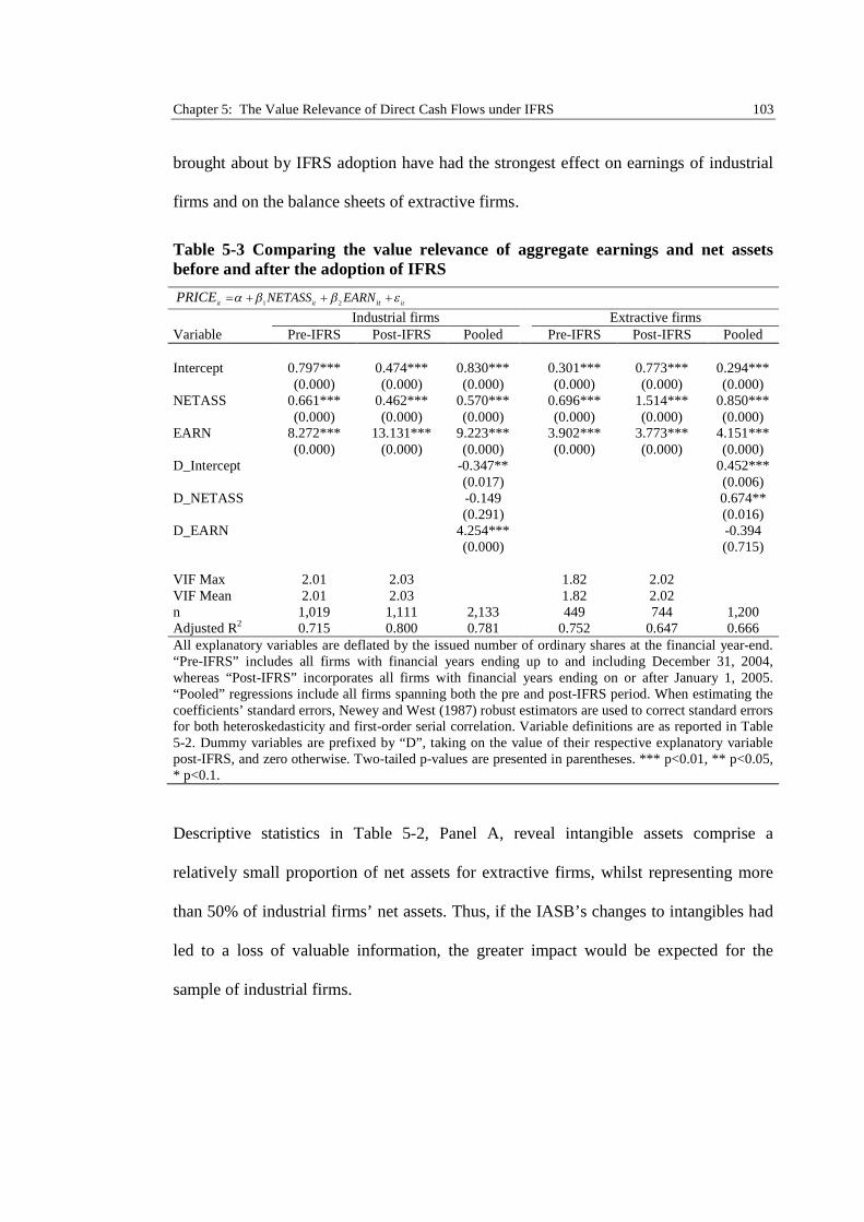
Chapter 5: The Value Relevance of Direct Cash Flows under IFRS 103
brought about by IFRS adoption have had the strongest effect on earnings of industrial
firms and on the balance sheets of extractive firms.
Table 5-3 Comparing the value relevance of aggregate earnings and net assetsbefore and after the adoption of IFRS
1 2
it it ititNETASS EARNPRICE
Industrial firms Extractive firmsVariable Pre-IFRS Post-IFRS Pooled Pre-IFRS Post-IFRS Pooled
Intercept 0.797*** 0.474*** 0.830*** 0.301*** 0.773*** 0.294***(0.000) (0.000) (0.000) (0.000) (0.000) (0.000)
NETASS 0.661*** 0.462*** 0.570*** 0.696*** 1.514*** 0.850***(0.000) (0.000) (0.000) (0.000) (0.000) (0.000)
EARN 8.272*** 13.131*** 9.223*** 3.902*** 3.773*** 4.151***(0.000) (0.000) (0.000) (0.000) (0.000) (0.000)
D_Intercept -0.347** 0.452***(0.017) (0.006)
D_NETASS -0.149 0.674**(0.291) (0.016)
D_EARN 4.254*** -0.394(0.000) (0.715)
VIF Max 2.01 2.03 1.82 2.02VIF Mean 2.01 2.03 1.82 2.02n 1,019 1,111 2,133 449 744 1,200Adjusted R2 0.715 0.800 0.781 0.752 0.647 0.666All explanatory variables are deflated by the issued number of ordinary shares at the financial year-end.“Pre-IFRS” includes all firms with financial years ending up to and including December 31, 2004,whereas “Post-IFRS” incorporates all firms with financial years ending on or after January 1, 2005.“Pooled” regressions include all firms spanning both the pre and post-IFRS period. When estimating thecoefficients’ standard errors, Newey and West (1987) robust estimators are used to correct standard errorsfor both heteroskedasticity and first-order serial correlation. Variable definitions are as reported in Table5-2. Dummy variables are prefixed by “D”, taking on the value of their respective explanatory variablepost-IFRS, and zero otherwise. Two-tailed p-values are presented in parentheses. *** p<0.01, ** p<0.05,* p<0.1.
Descriptive statistics in Table 5-2, Panel A, reveal intangible assets comprise a
relatively small proportion of net assets for extractive firms, whilst representing more
than 50% of industrial firms’ net assets. Thus, if the IASB’s changes to intangibles had
led to a loss of valuable information, the greater impact would be expected for the
sample of industrial firms.
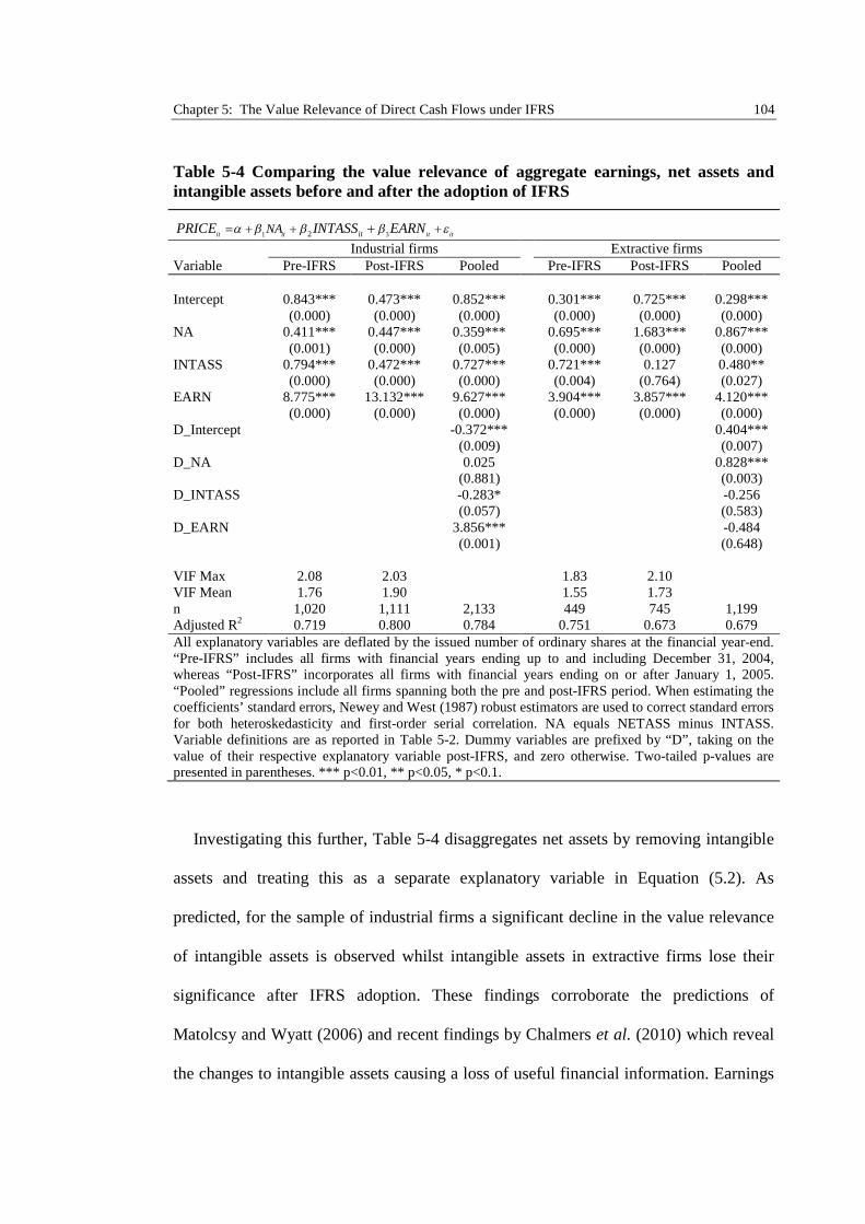
Chapter 5: The Value Relevance of Direct Cash Flows under IFRS 104
Table 5-4 Comparing the value relevance of aggregate earnings, net assets andintangible assets before and after the adoption of IFRS
1 32 it it it ititNAPRICE I EARNNTASS
Industrial firms Extractive firmsVariable Pre-IFRS Post-IFRS Pooled Pre-IFRS Post-IFRS Pooled
Intercept 0.843*** 0.473*** 0.852*** 0.301*** 0.725*** 0.298***(0.000) (0.000) (0.000) (0.000) (0.000) (0.000)
NA 0.411*** 0.447*** 0.359*** 0.695*** 1.683*** 0.867***(0.001) (0.000) (0.005) (0.000) (0.000) (0.000)
INTASS 0.794*** 0.472*** 0.727*** 0.721*** 0.127 0.480**(0.000) (0.000) (0.000) (0.004) (0.764) (0.027)
EARN 8.775*** 13.132*** 9.627*** 3.904*** 3.857*** 4.120***(0.000) (0.000) (0.000) (0.000) (0.000) (0.000)
D_Intercept -0.372*** 0.404***(0.009) (0.007)
D_NA 0.025 0.828***(0.881) (0.003)
D_INTASS -0.283* -0.256(0.057) (0.583)
D_EARN 3.856*** -0.484(0.001) (0.648)
VIF Max 2.08 2.03 1.83 2.10VIF Mean 1.76 1.90 1.55 1.73n 1,020 1,111 2,133 449 745 1,199Adjusted R2 0.719 0.800 0.784 0.751 0.673 0.679All explanatory variables are deflated by the issued number of ordinary shares at the financial year-end.“Pre-IFRS” includes all firms with financial years ending up to and including December 31, 2004,whereas “Post-IFRS” incorporates all firms with financial years ending on or after January 1, 2005.“Pooled” regressions include all firms spanning both the pre and post-IFRS period. When estimating thecoefficients’ standard errors, Newey and West (1987) robust estimators are used to correct standard errorsfor both heteroskedasticity and first-order serial correlation. NA equals NETASS minus INTASS.Variable definitions are as reported in Table 5-2. Dummy variables are prefixed by “D”, taking on thevalue of their respective explanatory variable post-IFRS, and zero otherwise. Two-tailed p-values arepresented in parentheses. *** p<0.01, ** p<0.05, * p<0.1.
Investigating this further, Table 5-4 disaggregates net assets by removing intangible
assets and treating this as a separate explanatory variable in Equation (5.2). As
predicted, for the sample of industrial firms a significant decline in the value relevance
of intangible assets is observed whilst intangible assets in extractive firms lose their
significance after IFRS adoption. These findings corroborate the predictions of
Matolcsy and Wyatt (2006) and recent findings by Chalmers et al. (2010) which reveal
the changes to intangible assets causing a loss of useful financial information. Earnings
Chapter 5: The Value Relevance of Direct Cash Flows under IFRS 105
are still found to increase in value relevance for industrial firms while net assets
increase in value relevance for extractive firms after the introduction of IFRS. IFRS has
therefore caused a significant loss of value relevant information from the balance sheet
for both industrial and extractive firms, due to the changes in accounting for intangible
assets.
5.5.2 Disaggregating Earnings
By disaggregating earnings into its constituent parts, Table 5-5 to 5-8 present results for
testing H1 and H2 by investigating the value relevance of operating cash flows and
direct cash flow components pre and post-IFRS. Table 5-5 presents the results of
Equation (5.3) which disaggregates earnings into operating cash flows and accruals
(Sloan, 1996). In line with the significant increase in value relevance of earnings for
industrial firms, support for H1 is found as a correspondingly significant rise in the
value relevance of operating cash flows is observed. Pre-IFRS, the mean coefficient for
operating cash flows is significant and positive for industrial firms. Moreover, the value
relevance post-IFRS of operating cash flows in the pooled regression reveals a
significant increase in the importance of operating cash flows in explaining firm value.
Likewise, accruals, which are significantly positive under AGAAP and IFRS, also
increased in value relevance for industrial firms under IFRS.
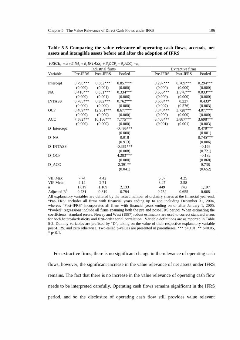
Chapter 5: The Value Relevance of Direct Cash Flows under IFRS 106
Table 5-5 Comparing the value relevance of operating cash flows, accruals, netassets and intangible assets before and after the adoption of IFRS
21 3 4
it it it it it itNA OCF ACCPRICE INTASS
Industrial firms Extractive firmsVariable Pre-IFRS Post-IFRS Pooled Pre-IFRS Post-IFRS Pooled
Intercept 0.798*** 0.362*** 0.857*** 0.297*** 0.789*** 0.294***(0.000) (0.001) (0.000) (0.000) (0.000) (0.000)
NA 0.416*** 0.351*** 0.334*** 0.656*** 1.576*** 0.833***(0.000) (0.001) (0.006) (0.000) (0.000) (0.000)
INTASS 0.785*** 0.382*** 0.762*** 0.668*** 0.227 0.433*(0.000) (0.000) (0.000) (0.007) (0.576) (0.063)
OCF 8.489*** 12.961*** 8.677*** 3.840*** 3.728*** 4.077***(0.000) (0.000) (0.000) (0.000) (0.000) (0.000)
ACC 7.582*** 10.166*** 7.775*** 3.403*** 3.887*** 3.698***(0.000) (0.000) (0.000) (0.001) (0.001) (0.003)
D_Intercept -0.495*** 0.479***(0.000) (0.001)
D_NA 0.018 0.745***(0.913) (0.006)
D_INTASS -0.381*** -0.163(0.008) (0.721)
D_OCF 4.283*** -0.182(0.000) (0.868)
D_ACC 2.391** 0.738(0.041) (0.652)
VIF Max 7.74 4.42 6.07 4.25VIF Mean 4.14 2.71 3.47 2.58n 1,019 1,109 2,133 449 743 1,197Adjusted R2 0.731 0.819 0.794 0.752 0.655 0.668All explanatory variables are deflated by the issued number of ordinary shares at the financial year-end.“Pre-IFRS” includes all firms with financial years ending up to and including December 31, 2004,whereas “Post-IFRS” incorporates all firms with financial years ending on or after January 1, 2005.“Pooled” regressions include all firms spanning both the pre and post-IFRS period. When estimating thecoefficients’ standard errors, Newey and West (1987) robust estimators are used to correct standard errorsfor both heteroskedasticity and first-order serial correlation. Variable definitions are as reported in Table5-2. Dummy variables are prefixed by “D”, taking on the value of their respective explanatory variablepost-IFRS, and zero otherwise. Two-tailed p-values are presented in parentheses. *** p<0.01, ** p<0.05,* p<0.1.
For extractive firms, there is no significant change in the relevance of operating cash
flows, however, the significant increase in the value relevance of net assets under IFRS
remains. The fact that there is no increase in the value relevance of operating cash flow
needs to be interpreted carefully. Operating cash flows remains significant in the IFRS
period, and so the disclosure of operating cash flow still provides value relevant
Chapter 5: The Value Relevance of Direct Cash Flows under IFRS 107
information for extractive firms. This may also be driven by the rise in the number of
extractive firms compared with industrial firms in the post-IFRS sample period. 34
Consequently, and as noted previously, firms within this industry often experience a
lengthy period with no or little operating cash flows whilst they are still in the
exploration phase of their business cycle. Moreover, there is a large rise in the number
of extractive firms reporting negative operating cash flows post-IFRS, up from 40%
under AGAAP to 51% under IFRS. The increased number of new extractive firms’
post-IFRS with very low and negative cash flows may explain, therefore, why there is
no increase in value relevance of operating cash flows. Alternatively, however, net
assets reported under IFRS may capture incremental information, which is reflected in
prices for extractive firms, as the assets of these firms give an indication of future
profitability once they are in the extraction phase.
In sum, these results present evidence that operating cash flows are value relevant
pre and post-IFRS and that there is a significant increase in the value relevance of
operating cash flows for industrial firms. The first hypotheses, H1, can therefore be
accepted for the sample of industrial firms that the value relevance of operating cash
flows increases under IFRS.
5.5.3 Disaggregating Cash Flows
Testing the second hypothesis H2, Equation (5.4) further disaggregates operating cash
flows into ‘core’ and ‘non-core’ direct cash flows. 35 Table 5-6, Panel A presents
34 Table 1, Panel A shows a significant rise in the number of Extractive firms in the post-IFRS periodfrom 2005-2010. Pre-2005 there is an average of 92 Extractive firms each year, whereas post-2004 thisaverage rises by 37% to 126 firms.35 Core operating cash flows are defined as the net of cash receipts from customers and cash payments tosuppliers and employees. Non-core cash flows are defined as interest paid, net taxes paid or refundsreceived, and all other operating cash flows.
Chapter 5: The Value Relevance of Direct Cash Flows under IFRS 108
findings consistent with the more parsimonious model used in Table 5-5, as there is a
significant increase in value relevance of both ‘core’ and ‘non-core’ operating cash
flows and accruals under IFRS for the sample of industrial firms. Further, for extractive
firms, core operating cash flows remain value relevant although there is a significant
decline in the value relevance of non-core operating cash flows under IFRS. Other than
the decline in value relevance of non-core operating cash flows for extractive firms,
these findings are in line with the observations made for net operating cash flows in
Table 5-5. Overall, however, these findings should be treated cautiously given the high
multicolinearity reported for industrial firms, as the VIF is greater than 10.
To address the problem of high multicolinearity reported in Table 5-6, Panel A, a
remedial measure recommended by Gujarati (1999) is followed by re-estimating
Equation (5.4) after dropping non-core operating cash flows, one of the collinear
variables. Non-core cash flows are chosen as the variable to be dropped as the focus of
the research question is on core cash flows, which can only be obtained from a direct
cash flow statement. Table 5-6, Panel B reports the results for the more restricted model
and the VIF are now less than 10, thereby addressing the problem with high
multicolinearity reported in Table 5-6, Panel A. Moreover, while the magnitude of the
coefficients for core direct cash flows and accruals are lower than those reported in
Table 5-6, Panel A, the findings presented in Table 5-6, Panel B, remain consistent with
those reported in Table 5-6, Panel A.
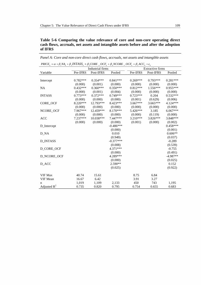
Chapter 5: The Value Relevance of Direct Cash Flows under IFRS 109
Table 5-6 Comparing the value relevance of core and non-core operating directcash flows, accruals, net assets and intangible assets before and after the adoptionof IFRS
Panel A: Core and non-core direct cash flows, accruals, net assets and intangible assets
2 31 4 5 _ _
it it it it it it itPRICE NA CORE OCF NCORE OCF ACCINTASS
Industrial firms Extractive firmsVariable Pre-IFRS Post-IFRS Pooled Pre-IFRS Post-IFRS Pooled
Intercept 0.782*** 0.354*** 0.841*** 0.269*** 0.793*** 0.281***(0.000) (0.001) (0.000) (0.000) (0.000) (0.000)
NA 0.432*** 0.360*** 0.350*** 0.812*** 1.556*** 0.955***(0.000) (0.001) (0.004) (0.000) (0.000) (0.000)
INTASS 0.773*** 0.372*** 0.749*** 0.723*** 0.204 0.532***(0.000) (0.000) (0.000) (0.001) (0.629) (0.006)
CORE_OCF 8.220*** 12.793*** 8.423*** 3.667*** 3.665*** 4.124***(0.000) (0.000) (0.000) (0.000) (0.000) (0.000)
NCORE_OCF 7.967*** 12.459*** 8.170*** 5.426*** 3.185 6.067***(0.000) (0.000) (0.000) (0.000) (0.119) (0.000)
ACC 7.237*** 10.038*** 7.447*** 3.210*** 3.826*** 3.848***(0.000) (0.000) (0.000) (0.001) (0.000) (0.002)
D_Intercept -0.486*** 0.458***(0.000) (0.001)
D_NA 0.010 0.606**(0.949) (0.037)
D_INTASS -0.377*** -0.289(0.008) (0.539)
D_CORE_OCF 4.371*** -0.755(0.000) (0.491)
D_NCORE_OCF 4.289*** -4.987**(0.000) (0.025)
D_ACC 2.590** 0.152(0.025) (0.922)
VIF Max 40.74 15.61 8.75 6.84VIF Mean 16.67 6.42 3.91 3.27n 1,019 1,109 2,133 450 743 1,195Adjusted R2 0.735 0.820 0.795 0.754 0.655 0.683
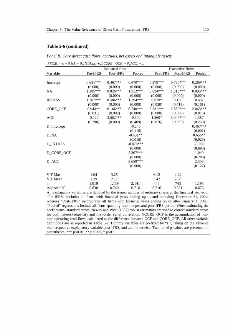
Chapter 5: The Value Relevance of Direct Cash Flows under IFRS 110
Table 5-6 (continued)
Panel B: Core direct cash flows, accruals, net assets and intangible assets
21 3 4 _
it it it it it itPRICE NA CORE OCF ACCINTASS
Industrial firms Extractive firmsVariable Pre-IFRS Post-IFRS Pooled Pre-IFRS Post-IFRS Pooled
Intercept 0.651*** 0.467*** 0.670*** 0.278*** 0.790*** 0.269***(0.000) (0.000) (0.000) (0.000) (0.000) (0.000)
NA 1.285*** 0.826*** 1.312*** 0.634*** 1.518*** 0.895***(0.000) (0.000) (0.000) (0.000) (0.000) (0.000)
INTASS 1.307*** 0.506*** 1.394*** 0.639* 0.156 0.432(0.000) (0.000) (0.000) (0.050) (0.718) (0.161)
CORE_OCF 0.943** 6.166*** 0.740*** 2.231*** 2.880*** 2.063***(0.031) (0.000) (0.000) (0.000) (0.000) (0.010)
ACC -0.120 3.582*** -0.302 1.360* 3.044*** 1.387(0.790) (0.000) (0.409) (0.076) (0.005) (0.250)
D_Intercept -0.245 0.467***(0.118) (0.001)
D_NA -0.431** 0.656**(0.016) (0.028)
D_INTASS -0.878*** -0.205(0.000) (0.698)
D_CORE_OCF 5.367*** 1.040(0.000) (0.280)
D_ACC 3.659*** 2.353(0.000) (0.127)
VIF Max 1.64 3.25 6.12 4.24VIF Mean 1.39 2.17 3.42 2.58n 1,019 1,119 2,141 448 743 1,195Adjusted R2 0.630 0.740 0.716 0.716 0.651 0.676All explanatory variables are deflated by the issued number of ordinary shares at the financial year-end.“Pre-IFRS” includes all firms with financial years ending up to and including December 31, 2004,whereas “Post-IFRS” incorporates all firms with financial years ending on or after January 1, 2005.“Pooled” regressions include all firms spanning both the pre and post-IFRS period. When estimating thecoefficients’ standard errors, Newey and West (1987) robust estimators are used to correct standard errorsfor both heteroskedasticity and first-order serial correlation. NCORE_OCF is the accumulation of non-core operating cash flows calculated as the difference between OCF and CORE_OCF. All other variabledefinitions are as reported in Table 5-2. Dummy variables are prefixed by “D”, taking on the value oftheir respective explanatory variable post-IFRS, and zero otherwise. Two-tailed p-values are presented inparentheses. *** p<0.01, ** p<0.05, * p<0.1.
Chapter 5: The Value Relevance of Direct Cash Flows under IFRS 111
Pooling data from different post-IFRS adoption years in Table 5-3 to 5-6 may mask
what could be a temporary change in value relevance. Accordingly, Equation (4),
restricted to exclude non-core operating cash flows to control for multicolinearity, is re-
estimated on an annual basis for both industrial and extractive firms, and the results
reported in Table 5-7. Consistent with a post-IFRS increase in value relevance for core
direct cash flows, there is a significant and sustained increase in the magnitude of the
coefficients for CORE_OCF for industrial firms for each year post-IFRS. Moreover, the
findings for extractive firms confirm an increase in value relevance of net assets post-
IFRS as evidenced by a significant increase in the interactive dummy variable NA in
four out of the six years between 2005 and 2010. These findings confirm the earlier
results, that the observed post-IFRS change in value relevance is significant and
persistent.
Overall, the findings from Table 5-6 and Table 5-7 provide strong initial support for
the value relevance of direct cash flows statements under IFRS across all industries.
Moreover, post-IFRS adoption, while remaining value relevant across all industries,
core direct cash flows significantly increase in value relevance for industrial firms.
Further, for industrial firms, non-core direct cash flow information, which would be
available in an indirect cash flow statement, is significantly more value relevant under
IFRS than AGAAP. Core direct cash flows evidently capture incremental information
which is reflected in prices for both industrial and extractive firms, but more so under
IFRS for industrial firms.
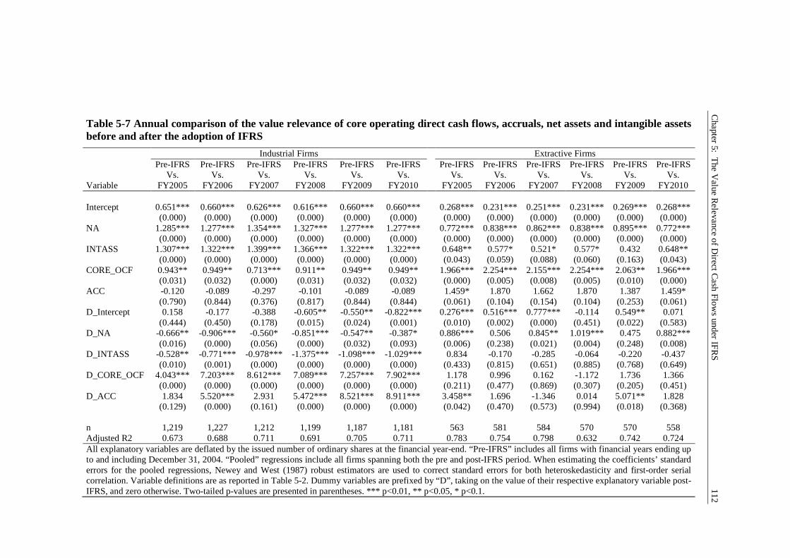
Chapter
5:T
heV
alueR
elevanceof
Direct
Cash
Flo
ws
und
erIF
RS
112
Table 5-7 Annual comparison of the value relevance of core operating direct cash flows, accruals, net assets and intangible assetsbefore and after the adoption of IFRS
Industrial Firms Extractive FirmsPre-IFRS Pre-IFRS Pre-IFRS Pre-IFRS Pre-IFRS Pre-IFRS Pre-IFRS Pre-IFRS Pre-IFRS Pre-IFRS Pre-IFRS Pre-IFRS
Vs. Vs. Vs. Vs. Vs. Vs. Vs. Vs. Vs. Vs. Vs. Vs.Variable FY2005 FY2006 FY2007 FY2008 FY2009 FY2010 FY2005 FY2006 FY2007 FY2008 FY2009 FY2010
Intercept 0.651*** 0.660*** 0.626*** 0.616*** 0.660*** 0.660*** 0.268*** 0.231*** 0.251*** 0.231*** 0.269*** 0.268***(0.000) (0.000) (0.000) (0.000) (0.000) (0.000) (0.000) (0.000) (0.000) (0.000) (0.000) (0.000)
NA 1.285*** 1.277*** 1.354*** 1.327*** 1.277*** 1.277*** 0.772*** 0.838*** 0.862*** 0.838*** 0.895*** 0.772***(0.000) (0.000) (0.000) (0.000) (0.000) (0.000) (0.000) (0.000) (0.000) (0.000) (0.000) (0.000)
INTASS 1.307*** 1.322*** 1.399*** 1.366*** 1.322*** 1.322*** 0.648** 0.577* 0.521* 0.577* 0.432 0.648**(0.000) (0.000) (0.000) (0.000) (0.000) (0.000) (0.043) (0.059) (0.088) (0.060) (0.163) (0.043)
CORE_OCF 0.943** 0.949** 0.713*** 0.911** 0.949** 0.949** 1.966*** 2.254*** 2.155*** 2.254*** 2.063** 1.966***(0.031) (0.032) (0.000) (0.031) (0.032) (0.032) (0.000) (0.005) (0.008) (0.005) (0.010) (0.000)
ACC -0.120 -0.089 -0.297 -0.101 -0.089 -0.089 1.459* 1.870 1.662 1.870 1.387 1.459*(0.790) (0.844) (0.376) (0.817) (0.844) (0.844) (0.061) (0.104) (0.154) (0.104) (0.253) (0.061)
D_Intercept 0.158 -0.177 -0.388 -0.605** -0.550** -0.822*** 0.276*** 0.516*** 0.777*** -0.114 0.549** 0.071(0.444) (0.450) (0.178) (0.015) (0.024) (0.001) (0.010) (0.002) (0.000) (0.451) (0.022) (0.583)
D_NA -0.666** -0.906*** -0.560* -0.851*** -0.547** -0.387* 0.886*** 0.506 0.845** 1.019*** 0.475 0.882***(0.016) (0.000) (0.056) (0.000) (0.032) (0.093) (0.006) (0.238) (0.021) (0.004) (0.248) (0.008)
D_INTASS -0.528** -0.771*** -0.978*** -1.375*** -1.098*** -1.029*** 0.834 -0.170 -0.285 -0.064 -0.220 -0.437(0.010) (0.001) (0.000) (0.000) (0.000) (0.000) (0.433) (0.815) (0.651) (0.885) (0.768) (0.649)
D_CORE_OCF 4.043*** 7.203*** 8.612*** 7.089*** 7.257*** 7.902*** 1.178 0.996 0.162 -1.172 1.736 1.366(0.000) (0.000) (0.000) (0.000) (0.000) (0.000) (0.211) (0.477) (0.869) (0.307) (0.205) (0.451)
D_ACC 1.834 5.520*** 2.931 5.472*** 8.521*** 8.911*** 3.458** 1.696 -1.346 0.014 5.071** 1.828(0.129) (0.000) (0.161) (0.000) (0.000) (0.000) (0.042) (0.470) (0.573) (0.994) (0.018) (0.368)
n 1,219 1,227 1,212 1,199 1,187 1,181 563 581 584 570 570 558Adjusted R2 0.673 0.688 0.711 0.691 0.705 0.711 0.783 0.754 0.798 0.632 0.742 0.724All explanatory variables are deflated by the issued number of ordinary shares at the financial year-end. “Pre-IFRS” includes all firms with financial years ending upto and including December 31, 2004. “Pooled” regressions include all firms spanning both the pre and post-IFRS period. When estimating the coefficients’ standarderrors for the pooled regressions, Newey and West (1987) robust estimators are used to correct standard errors for both heteroskedasticity and first-order serialcorrelation. Variable definitions are as reported in Table 5-2. Dummy variables are prefixed by “D”, taking on the value of their respective explanatory variable post-IFRS, and zero otherwise. Two-tailed p-values are presented in parentheses. *** p<0.01, ** p<0.05, * p<0.1.
Chapter 5: The Value Relevance of Direct Cash Flows under IFRS 113
Table 5-8 presents the results for Equation (5.5), which has the highest level of cash
flow disaggregation. Given Equation (5.5) has by design two highly collinear variables,
CSHRC and CSHPS, this final model naturally suffers from high multicolinearity.
However, for completeness, and in order to be consistent with Clinch et al. (2002), the
results of Equation (5.5) are reported, but these are only presented for consistency with
prior research. The results show that direct cash flow components, with the exception of
tax (TXP), are value relevant both pre and post-IFRS for the sample of industrial firms.
Moreover, the mean coefficients for the interactive dummy variables show a significant
increase in the value relevance of the two ‘core’ direct cash flow measures, namely,
cash receipts from customers (CSHRC) and payments to suppliers and employees
(CSHPS). Interest paid (INTP) and other operating cash flows (CSHOTH) increase in
value relevance under IFRS. Accruals (ACC) are also found to be value relevant for
industrial and extractive firms under both AGAAP and IFRS, but there is no increase in
relevance since the adoption of IFRS.
Much like industrial firms, the direct cash flow components for the sample of
extractive firms all reveal a strong association with the share price under both AGAAP
and IFRS, with the exception of INTP and TXP, which are insignificant at levels less
than 5% post-IFRS. However, in contrast to the findings for industrial firms, based on
the dummy variables from the pooled regressions for extractive firms, adopting IFRS
has only resulted in a significant change in the value relevance of CSHOTH after the
adoption of IFRS. Consistent, with a rise in the number of extractive firms, as shown in
Table 5-2, reporting positive other operating cash flows (CSHOTH) pre-IFRS, but
negative CSHOTH under IFRS, there is a change in signs of the coefficient for net other
operating cash flows.
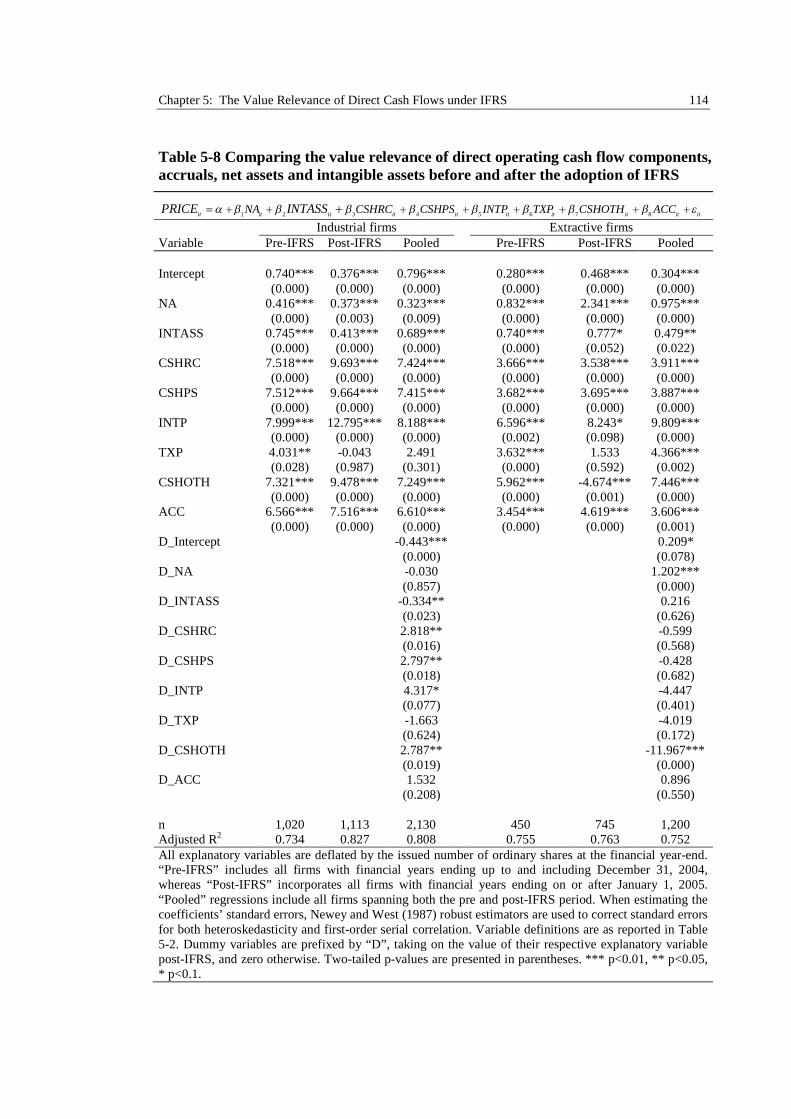
Chapter 5: The Value Relevance of Direct Cash Flows under IFRS 114
Table 5-8 Comparing the value relevance of direct operating cash flow components,accruals, net assets and intangible assets before and after the adoption of IFRS
2 3 4 5 6 71 8
it it it it it it it it it itNA CSHRC CSHPS INTP TXP CSHOTH ACCPRICE INTASS
Industrial firms Extractive firmsVariable Pre-IFRS Post-IFRS Pooled Pre-IFRS Post-IFRS Pooled
Intercept 0.740*** 0.376*** 0.796*** 0.280*** 0.468*** 0.304***(0.000) (0.000) (0.000) (0.000) (0.000) (0.000)
NA 0.416*** 0.373*** 0.323*** 0.832*** 2.341*** 0.975***(0.000) (0.003) (0.009) (0.000) (0.000) (0.000)
INTASS 0.745*** 0.413*** 0.689*** 0.740*** 0.777* 0.479**(0.000) (0.000) (0.000) (0.000) (0.052) (0.022)
CSHRC 7.518*** 9.693*** 7.424*** 3.666*** 3.538*** 3.911***(0.000) (0.000) (0.000) (0.000) (0.000) (0.000)
CSHPS 7.512*** 9.664*** 7.415*** 3.682*** 3.695*** 3.887***(0.000) (0.000) (0.000) (0.000) (0.000) (0.000)
INTP 7.999*** 12.795*** 8.188*** 6.596*** 8.243* 9.809***(0.000) (0.000) (0.000) (0.002) (0.098) (0.000)
TXP 4.031** -0.043 2.491 3.632*** 1.533 4.366***(0.028) (0.987) (0.301) (0.000) (0.592) (0.002)
CSHOTH 7.321*** 9.478*** 7.249*** 5.962*** -4.674*** 7.446***(0.000) (0.000) (0.000) (0.000) (0.001) (0.000)
ACC 6.566*** 7.516*** 6.610*** 3.454*** 4.619*** 3.606***(0.000) (0.000) (0.000) (0.000) (0.000) (0.001)
D_Intercept -0.443*** 0.209*(0.000) (0.078)
D_NA -0.030 1.202***(0.857) (0.000)
D_INTASS -0.334** 0.216(0.023) (0.626)
D_CSHRC 2.818** -0.599(0.016) (0.568)
D_CSHPS 2.797** -0.428(0.018) (0.682)
D_INTP 4.317* -4.447(0.077) (0.401)
D_TXP -1.663 -4.019(0.624) (0.172)
D_CSHOTH 2.787** -11.967***(0.019) (0.000)
D_ACC 1.532 0.896(0.208) (0.550)
n 1,020 1,113 2,130 450 745 1,200Adjusted R2 0.734 0.827 0.808 0.755 0.763 0.752All explanatory variables are deflated by the issued number of ordinary shares at the financial year-end.“Pre-IFRS” includes all firms with financial years ending up to and including December 31, 2004,whereas “Post-IFRS” incorporates all firms with financial years ending on or after January 1, 2005.“Pooled” regressions include all firms spanning both the pre and post-IFRS period. When estimating thecoefficients’ standard errors, Newey and West (1987) robust estimators are used to correct standard errorsfor both heteroskedasticity and first-order serial correlation. Variable definitions are as reported in Table5-2. Dummy variables are prefixed by “D”, taking on the value of their respective explanatory variablepost-IFRS, and zero otherwise. Two-tailed p-values are presented in parentheses. *** p<0.01, ** p<0.05,* p<0.1.
Chapter 5: The Value Relevance of Direct Cash Flows under IFRS 115
Taken as a whole, these findings provide strong evidence of direct cash flows
reported under IFRS capturing incremental information which is reflected in the stock
prices. Specifically, ‘core’ cash flows that are unavailable under indirect cash flow
statements are value relevant and reflected in share price across all industries. Further,
‘core’ direct cash flows at the very least remain value relevant after the move to IFRS,
and for industrial firms they are shown to increase significantly in value relevance
under IFRS. The second hypothesis H2 can therefore be accepted, that there will be a
rise in the value relevance of direct cash flow components under IFRS.
5.5.4 Robustness Tests
Although Australian firms were prohibited from full early voluntary adoption of IFRS,
they were required to report on the impact of adopting IFRS in their 2005 financial
statements. To account for the release of this information to investors in 2005, firm-year
observations were included from this year as part of the post-IFRS sample period.
However, in order to test the robustness of the findings all 2005 firm-year observations
were dropped in following Jones and Finley (2011). The results for all of the models
remained consistent with the above findings. In addition, all the analysis was re-
estimated to include industry level dummies in all the models to control for any
unobserved industry group effects. Once more, the results of the analysis including
industry controls remain qualitatively similar to the above findings. Finally, Wald tests
were used to examine the change in value relevance of direct cash flow disclosures and
the results are consistent with those presented above.
Chapter 5: The Value Relevance of Direct Cash Flows under IFRS 116
5.6 Conclusions
Currently, the IASB and FASB are proposing that direct cash flow statements become
mandatory for all companies under their harmonised cash flow reporting joint project.
While there is strong academic evidence to support the mandating of direct cash flow
statements given their usefulness to users of accounts (e.g., Jones et al., 1995; Clinch et
al., 2002; Goyal, 2004), there are a number of critics of the proposal to mandate the
direct method given the cost of disclosure (Hales and Orpurt, 2012). This chapter
therefore analyses whether direct cash flow disclosures remain value relevant for a
sample of Australian firms, to test whether direct cash flow statements continue to
capture the rich information set reflected in stock prices in an IFRS reporting
environment.
The results provide strong evidence that direct cash flow statements are a value
relevant disclosure under AGAAP and IFRS, and that this result holds for both
industrial and extractive firms. Moreover, for the sample of industrial firms the findings
reveal that there has been an increase in the value relevance of direct cash flows since
the adoption of IFRS. In addition, ‘core’ and ‘non-core’ cash flow disclosures are found
to increase in value relevance for industrial firms under IFRS. Consequently, if the
IASB were to mandate direct cash flow statements it would, in all likelihood, provide
users of accounts with a valuable incremental source of information.
The observed increase in value relevance for industrial firms under IFRS is also
consistent with increased uncertainty around the accounting numbers that are being
disclosed. Based upon the evidence of Bissessur and Hodgson (2011), the move to IFRS
created a degree of uncertainty in the accounting numbers being disclosed. In particular,
and consistent with Chalmers et al. (2010), for industrial firms the findings provides
Chapter 5: The Value Relevance of Direct Cash Flows under IFRS 117
evidence that IFRS has resulted in a loss of value relevant information regarding
intangibles. As a result, an increase in the value relevance of direct cash flow numbers
is unsurprising in times of uncertainty. In addition, the sample period also includes one
of the biggest periods of uncertainty in recent times, namely the financial crisis, and so
a continued reliance on direct cash flow numbers is again unsurprising. Ultimately,
whether the increased value relevance on direct cash flow numbers persists beyond the
current market turmoil would merit future investigation. Regardless of this, the findings
in this chapter present strong evidence that direct cash flow disclosures are value
relevant in an IFRS reporting environment.
While this chapter provides strong evidence that direct cash flow statements provide
investors with useful information under AGAAP and IFRS, survey results by the CFA
Institute also show financial analysts are a significant proponent of direct cash flow
statements. Analysts’ assert that direct cash flow statements provide useful information
when forecasting future cash flows. Moreover, these survey results have provided the
IASB and FASB with strong evidence to support their proposal to mandate direct cash
flow statements. Accordingly, the subsequent empirical chapter examines whether
financial analysts use information from direct cash flow statements when forecasting
cash flows under AGAAP and IFRS. Further, Chapter 6 investigates whether analysts
find information from direct cash flow statements more useful for forecasting cash
flows under IFRS, when compared to AGAAP.
Chapter 6: Direct Cash Flow Statements and Analyst Cash Flow Forecast Accuracy under IFRS 118
6Direct Cash Flow Statements and AnalystCash Flow Forecast Accuracy under IFRS
6.1 Introduction
The recent proposal by the International Accounting Standards Board (IASB) and
Financial Accounting Standards Board (FASB) to mandate direct cash flow statements
received strong support from financial analysts.36 Survey results conducted by the CFA
Institute show most analysts believe direct cash flow statements provide better
information for forecasting future cash flows and measuring earnings quality than
indirect cash flow statements. 37 These results are unsurprising given the strong
empirical evidence which shows direct cash flow statements provide incremental
information when forecasting future cash flows under local Generally Accepted
Accounting Principles (GAAP) (e.g., Krishnan and Largay III, 2000; Orpurt and Zang,
2009; Arthur et al., 2010; Farshadfar and Monem, 2012, 2013). However, although
these studies advocate direct cash flow reporting, the more recent studies do so after
specifically excluding all observations since the adoption of International Financial
Reporting Standards (IFRS), reasoning that financial reports under IFRS were
significantly different to local GAAP (Arthur et al., 2010; Farshadfar and Monem, 2012,
2013). This reasoning was a priori confirmed by the Australian Accounting Standards
Board (AASB) who predicted IFRS would significantly change financial reporting and
benefit users by providing relevant and reliable financial information (Fenton-Jones,
36 See the FASB Proposed Accounting Standards Update published in July 2010 (paragraph 177).37 See the CFA Institute Member Poll: Cash Flow Survey published in 2009.
Chapter 6: Direct Cash Flow Statements and Analyst Cash Flow Forecast Accuracy under IFRS 119
2003). Providing further evidence of these changes, empirical studies found significant
improvements in the quality and comparability of Australian financial reports,
evidenced by a significant rise in the accuracy of analysts’ earnings forecasts under
IFRS (Bissessur and Hodgson, 2011; Cotter et al., 2012), which is consistent with other
international studies (e.g., Byard et al., 2011; Tan et al., 2011; Horton et al., 2012).
Examining the usefulness of direct cash flow statements to forecast cash flows under
IFRS would provide both the IASB and FASB empirical evidence, to assist with the
decision of whether or not direct cash flow reporting should be mandatory. Further,
while prior studies substantiate that direct cash flow components improve the accuracy
or explanatory power of random walk cash flow prediction models, to date, no research
has empirically tested whether financial analysts find this information useful when
predicting cash flows. A significant factor behind the motivation for the joint proposal
by the FASB and IASB to mandate direct cash flow statements is the recent CFA
Institute survey findings showing financial analysts’ strongly support the use of direct
cash flow statements. Whether financial analysts actually use direct cash flow
statements when predicting future cash flows, and whether this information remains
useful under IFRS, are the two questions that this chapter aims to address.
By using a sample of non-financial Australian companies listed on the ASX300 from
2000-2010 this chapter examines whether analysts find direct cash flow statements
useful when predicting annual cash flows, and whether this has changed under IFRS
compared to local GAAP. Moreover, this chapter examines whether the accuracy of
analysts’ cash flow predictions has improved under IFRS, and if the improvement is
associated with an increased use of direct cash flow components. Australia provides an
ideal context in which to test these questions since the use of direct cash flow
Chapter 6: Direct Cash Flow Statements and Analyst Cash Flow Forecast Accuracy under IFRS 120
statements was mandatory until 2007, after which most firms continued to use this
approach for the remainder of the sample period. Further, Australian firms were
prohibited from early adoption of IFRS, and so all firms commenced reporting under
IFRS for fiscal years beginning on or after 1 January 2005. There is, therefore, a distinct
break in time, which permits the examination of analysts’ use of direct cash flow
statements before and after IFRS adoption, and whether analysts’ cash flow forecast
errors change under IFRS.
The main findings show financial analysts do use information from direct cash flow
statements when predicting annual cash flows across the entire sample period and
significantly more so under IFRS. Further, analyst cash flow forecast errors are shown
to significantly decline under IFRS, suggesting that IFRS adoption improved the quality
of analysts’ information environment. Taken together, these findings support the
assertion made by standard setters and analysts that direct cash flow statements provide
useful information for predicting cash flows. This suggests that the proposal of the
IASB and FASB is not without its merits, and if implemented could further improve the
information environment for users of financial accounts.
6.2 Background and Hypothesis Development
6.2.1 Direct Cash Flows and Forecasting
Since cash flow reporting requirements were standardised three decades ago, on-going
debates have focussed on the benefits of reporting operating cash flows using the direct
method. Academics have generally favoured the direct method (e.g., Jones et al., 1995;
McEnroe, 1996; Smith and Freeman, 1996; Jones and Ratnatunga, 1997; Jones and
Widjaja, 1998; Goyal, 2004). Moreover, standard setters have asserted that information
Chapter 6: Direct Cash Flow Statements and Analyst Cash Flow Forecast Accuracy under IFRS 121
from direct cash flow statements is useful when forecasting future cash flows. 38
Nevertheless, Australia, New Zealand and China are historically the only countries that
required the mandatory use of direct cash flow statements (Wallace et al., 1997; Clinch
et al., 2002).39 All other nations, which provided a choice between the two approaches,
found most companies applied the indirect approach.40 The recent IASB/FASB proposal
to mandate the use of direct cash flow statements has therefore provoked a significant
response. 41 Based on the comment letters, it is evident that most preparers remain
unconvinced about the stated benefits of direct cash flow reporting, especially given the
perceived high costs of changing information systems to capture this information.42
However, in contrast to this feedback, a recent survey conducted by the Institute of
Chartered Financial Analysts (CFA Institute) found most respondents were in favour of
mandating the use of direct cash flow statements. 63% ‘strongly agreed’ or ‘agreed’
that information from direct cash flow statements could improve analyst cash flow
forecast accuracy and would also provide useful measures of earnings quality. Further,
94% voted ‘Revenue collections from customers’, which is only reported in direct cash
flow statements, to be the most important information disclosed as part of cash flows
from operating activities.43 This supports the arguments put forward by academics,
which note the theoretical superiority of direct cash flow statements by arguing this
38 See for example, U.S. accounting standard SFAS 95: Statement of Cash Flows, issued in 1987(paragraph 107), or the International Accounting Standards Board (IASB) standard IAS 7: Statement ofCash Flows, issued up to 2009 (paragraph 19), and Australian accounting standard AASB 1026:Statement of Cash Flows, issued in 1997(paragraph 6.2.2).39 In 2007 the AASB amended AASB 107: Statement of Cash Flows by issuing Amendments toAustralian Accounting Standards 2007-4 allowing firms the choice of reporting operating cash flowsindirectly thereby aligning themselves with IFRS.40 Orpurt and Zang (2009) reveal that less than 2% of all firms in America currently use the directmethod.41 See the FASB Proposed Accounting Standards Update published in July 2010 (paragraph 177).42 See the comment letters from the FASB Preliminary Views on Financial Statement PresentationReference Number: 1630-100 published in 2009.43 See the CFA Institute Member Poll: Cash Flow Survey published in 2009.
Chapter 6: Direct Cash Flow Statements and Analyst Cash Flow Forecast Accuracy under IFRS 122
method to be less confusing (Paton, 1963), providing better information (Thomas, 1982),
and having better linkage to the income statement (Ketz and Largay III, 1987),
compared to the indirect method. Moreover, and consistent with the recent CFA
institute findings, direct cash flow statements were also asserted to provide useful
information for credit analysis (Heath, 1978).
Empirically examining the usefulness of direct cash flow information, Livnat and
Zarowin (1990) provide the first evidence for the value relevance of direct cash flows.
By estimating direct cash flow components, they find a significant association between
abnormal stock returns and unexpected changes in direct cash flow components.
Extending this study, Clinch et al. (2002) use a sample of Australian firms providing
further evidence of the value relevance of direct cash flows. By using actual, rather than
estimated, direct cash flow components, they find annual stock returns are better
explained by direct cash flow components, compared to aggregate operating cash flows,
when controlling for their ability to predict future operating cash flows.
These results corroborate earlier findings by Krishnan and Largay III (2000) who
also find strong evidence in support of the widely held belief that direct cash flow
statements provide useful information for predicting next year’s cash flows. By using a
sample of U.S. firms voluntarily reporting direct cash flows, their results show an
increased accuracy for their cash flow prediction models after including direct cash flow
components as explanatory variables. Providing further support for the predictive power
of direct cash flow statements, subsequent U.S. (Cheng and Hollie, 2008; Orpurt and
Zang, 2009), and Australian (Arthur and Chuang, 2008; Arthur et al., 2010) studies also
confirm a significant increase in accuracy and explanatory power after including
estimated or reported direct cash flow components in their models. However, despite
Chapter 6: Direct Cash Flow Statements and Analyst Cash Flow Forecast Accuracy under IFRS 123
these findings affirming the usefulness of direct cash flow statements, there is no known
study that has investigated whether analysts’ use information from direct cash flow
statements to predict future cash flows.
6.2.2 Analysts’ Use of Direct Cash Flow Components
Providing cash flow forecasts alongside earnings forecasts is a relatively new and
growing phenomenon. DeFond and Hung (2007) sample more than 70,000 earnings
forecasts from 36 countries. These results show a rise in the number of earnings
forecasts being accompanied by cash flow forecasts up from only 30% in 1994 to 58%
in 2002. Examining this trend, DeFond and Hung (2003) find that analysts issue cash
flow forecasts as a complement to their earnings forecasts in response to market
demand for price relevant information for firms with volatile earnings, high accruals,
and poor financial health. Further, issuing both earnings and cash flow forecasts is
found to significantly increase the accuracy of analysts’ earnings forecasts (Call et al.,
2009), whilst at the same time providing an external deterrent to managers undertaking
earnings management (Call, 2008; McInnis and Collins, 2011).
There is, however, debate as to whether analysts’ cash flow forecasts are really a
sophisticated projection of future cash flows (DeFond and Hung, 2003; Call et al., 2012)
or rather a simple adjustment of their earnings forecast (Givoly et al., 2009). Although
Givoly et al. (2009) and Call et al. (2012) argue the sophistication of analysts cash flow
forecasts, both agree that analysts cash flow forecasts outperform the more mechanical
Barth et al. (2001b) time series prediction models based on lagged earnings components.
Further evidence for the sophistication of analysts cash flow forecasts is provided by
Call et al. (2012), when analysing random samples of full text analyst reports. Their
analysis showed 80% of analysts considered working capital and other accrual
Chapter 6: Direct Cash Flow Statements and Analyst Cash Flow Forecast Accuracy under IFRS 124
adjustments when predicting cash flows. However, to date, extant research examining
the sophistication of analysts’ cash flow forecasts assumes analysts use information
from indirect cash flow statements as much of this research is based in the U.S. (e.g.,
DeFond and Hung, 2003; Call et al., 2012).
Investigating whether the layout of operating cash flows would influence the
accuracy of cash flow predictions, Hodder et al. (2008) exploit an experimental setting
of 50 business graduates, providing them with either an indirect cash flow statement
which reconciles net income to operating cash flows, or, the same information, but this
time reconciling operating cash flows to net income. Their results show significantly
higher forecast errors and dispersion in the sample of graduates using traditional
indirect cash flow statements, implying that the structure of operating cash flows can
significantly affect users’ abilities to forecast cash flows accurately. This may explain
why feedback from the 2009 CFA Institute survey show financial analysts agree that
information from direct cash flow statements would improve the accuracy of future cash
flow forecasts, and provides motivation for the first hypothesis:
H1: Analysts will find direct cash flow components useful in forecasting future cash
flows.
6.2.3 IFRS Adoption and Analysts’ Use of Direct Cash Flow Components
Both prior to the adoption of IFRS in 2005, and for two years subsequently, Australia
mandated the use of direct cash flow statements until, in 2007, they provided the option
of using an indirect cash flow statement. Before Australia’s adoption of IFRS, there
were already signs from European markets that investors anticipated the mandatory
European Union (E.U.) wide adoption of IFRS would improve the information set
reported by firms under the new standards (Armstrong et al., 2010). This was shown by
Chapter 6: Direct Cash Flow Statements and Analyst Cash Flow Forecast Accuracy under IFRS 125
a series of positive European market reactions following announcements for the
mandatory adoption of IFRS in the E.U. Subsequently, E.U. and Australian studies
corroborated these investor sentiments finding a general reduction in cost of capital and
improved capital market liquidity after the mandatory adoption of IFRS (Daske et al.,
2008). While there was concern that, under IFRS, fair value accounting would increase
earnings volatility (Ball, 2006), overall, annual reports prepared under IFRS appeared to
provide a richer information set than was previously available under local GAAP.
Daske et al. (2008), however, also noted that the increased market liquidity under
IFRS only occurred in countries with strong reporting incentives and legal enforcement
of accounting standards. This is consistent with the views of Ball (2006) and
Soderstrom and Sun (2007), who hypothesised, that, the effectiveness of the
enforcement of IFRS would significantly influence the perceived benefits associated
with adopting the new standards. Further, emphasising the important role of effective
enforcement after Europe’s mandatory adoption of IFRS, Byard et al.’s (2011) results
show analyst earnings forecast errors decline significantly, but only in countries with a
strong legal environment. Australia has a strong legal environment, and recent findings
show a significant increase in analysts’ earnings forecast accuracy under IFRS
(Bissessur and Hodgson, 2011; Cotter et al., 2012). These are consistent with the global
study, including Australia, of Horton et al. (2012), which also found significant
improvements in analysts’ information environment post-IFRS.
After the adoption of IFRS in Australia, Bissessur and Hodgson (2011) and Cotter et
al. (2012) state that the significant decline in analyst earnings forecast errors is a
consequence of IFRS providing Australian analysts with a far richer source of
information than was previously available. This is consistent with the view of analysts
Chapter 6: Direct Cash Flow Statements and Analyst Cash Flow Forecast Accuracy under IFRS 126
acting as information intermediaries who utilise a range of information sources, one of
which is the annual report, to arrive at their earnings and cash flow forecasts (Barth and
Hutton, 2004). However, Bissessur and Hodgson (2011) and Cotter et al. (2012), do not
consider the sources of information in the annual report that are used by analysts to
improve their forecasts.
Sloan (1996) identifies two key sources of information used by analysts in financial
accounts are historical accruals and operating cash flows, with operating cash flows
providing a useful source of information given their persistence. When Australia
adopted IFRS in 2005, there were no major changes to cash flow reporting between
AASB 1026, and the IFRS equivalent to IAS 7, AASB 107 Statement of Cash flows.
Australian cash flow disclosure requirements, therefore, have remained consistent under
both AGAAP and IFRS, while the reporting of net assets and earnings changed.
Given the consistency in reporting direct cash flows pre and post-IFRS, Australia
provides an ideal setting to examine how IFRS adoption may have changed the
usefulness of information from direct cash flow statements. Recent Australian studies,
examining the predictive power of direct cash flows, cited the significant changes to the
measurement of earnings and accruals under IFRS as reasons to exclude all
observations under IFRS (Arthur et al., 2010; Farshadfar and Monem, 2012, 2013).
However, excluding observations under IFRS fails to consider how the usefulness of
this information may have changed. While cash flow reporting requirements have
remained unchanged by the adoption of IFRS in Australia, Bissessur and Hodgson
(2011) and Cotter et al. (2012) find that there has been an overall improvement in
analysts’ ability to more accurately forecast earnings. If IFRS provides a richer
information set than previously available, the overall importance of direct cash flow
Chapter 6: Direct Cash Flow Statements and Analyst Cash Flow Forecast Accuracy under IFRS 127
information should also increase, as it is an established source of information for
financial analysts, which would be complemented by the improved information set
provided by IFRS when forecasting future cash flows. Accordingly, the next hypothesis
states:
H1b: Analysts will find direct cash flow components significantly more useful in
forecasting future cash flows after adopting IFRS.
6.2.4 IFRS Adoption and Analysts’ Information Environment
Investigating the impact of IFRS adoption on financial analysts earnings forecasts,
empirical studies conclude IFRS adoption improves analysts information environment
for predicting earnings, as evidenced by increased forecast accuracy after early
voluntary IFRS adoption (Ashbaugh and Pincus, 2001; Bae et al., 2008; Hodgdon et al.,
2008). Further, analyst earnings forecast errors also dropped significantly after the
mandatory adoption of IFRS, corroborating these findings within a mandatory adoption
framework (Bissessur and Hodgson, 2011; Cotter et al., 2012; Horton et al., 2012).
Moreover, the greatest improvements in the accuracy of analyst earnings forecasts were
found in countries with strong enforcement of accounting standards, and significant
differences between local GAAP and IFRS (Byard et al., 2011). Consistent with an
earlier study by Hope (2003), strong enforcement of the new accounting standards
allowed the IFRS accounts to provide financial analysts with a richer information set.
Chapter 6: Direct Cash Flow Statements and Analyst Cash Flow Forecast Accuracy under IFRS 128
Given Australia’s strong enforcement of accounting standards, and the notable44
differences between local GAAP and IFRS, recent studies have found a strong
improvement in the accuracy of earnings forecasts by Australian analysts (Bissessur and
Hodgson, 2011; Cotter et al., 2012). Prohibiting the voluntary adoption of IFRS, and
actively enforcing accounting standards, makes Australia an ideal country to examine
the impact of IFRS adoption on analysts’ information environment. However, while
studies provide strong evidence that IFRS adoption improved financial analysts’
information environment, they do so using changes in the accuracy of analysts’ earnings
forecasts as a proxy for information changes. To date, no research has considered
changes in the accuracy of analysts’ cash flow forecasts as an alternative proxy for
information changes. According to the IASB financial reporting framework, an
underlying objective of financial statements prepared according to IFRS is providing
users with information that will be useful in assessing an entities prospect of generating
future cash inflows.45 It follows, therefore, that if the adoption of IFRS has improved
analysts’ information environment, financial analysts would be expected to forecast
annual cash flows more accurately. Accordingly, the next hypothesis states:
H2: Analysts’ cash flow forecast errors will significantly reduce after adopting IFRS.
44 Some of the more significant differences between Australian GAAP and IFRS include: IFRSprohibiting the disclosure of extraordinary items; disallowing the use of the full liability method ofaccounting for deferred taxation; prohibiting the recognition of certain non-goodwill related internallygenerated intangible assets; accounting for changes in the fair value of investment properties through theincome statement rather than the statement of changes in equity; providing far more comprehensiverequirements and guidance for the recognition and disclosure of financial instruments; requiring therecognition and disclosure of all share based payments irrespective of whether they were applicable todirectors, executives or all staff. (Deloitte, Differences between current Australian GAAP and Australianequivalents to IFRS, published in August 2004).45 See paragraph OB3 of the September 2010 IFRS Foundation Conceptual Framework
Chapter 6: Direct Cash Flow Statements and Analyst Cash Flow Forecast Accuracy under IFRS 129
Comparing the forecast accuracy of different cash flow prediction models, Krishnan
and Largay III (2000) found the lowest mean absolute percentage error for the model
that included direct cash flow components. They conclude that historical direct cash
flow components provide more useful information than historical indirect cash flows
when predicting future cash flows. The previous hypotheses have considered whether
analysts use direct cash flow components to forecast cash flows, and if there has been a
significant increase in the use of direct cash flow components under IFRS. Further, H2
predicts an improvement in analysts’ information environment post-IFRS as evidenced
by reduced cash flow forecast errors. It follows, therefore, that should financial analysts
find direct cash flows useful, and even more so under IFRS, any improvement in
forecast accuracy under IFRS will be partly due to analysts’ increased use of direct cash
flow components. Accordingly, the final hypothesis states:
H2b: Improvements in analysts’ cash flow forecast accuracy post-IFRS will be
significantly associated with analysts’ increased use of direct cash flow
components post-IFRS.
6.3 Research Design and Sample Selection
6.3.1 Analysts’ Cash Flow Forecasts and Direct Cash Flow Components
Addressing the first hypotheses, the following equations modify the models used by
Krishnan and Largay (2000) and Barth et al. (2001b) by exploiting analysts median
consensus forecast of annual cash flows per share, rather than future reported operating
cash flows, as the dependent variable. This, therefore, allows the examination of
whether or not financial analysts’ forecasts are explained by historical cash flow
information. In order to examine the change in the usefulness of the information from
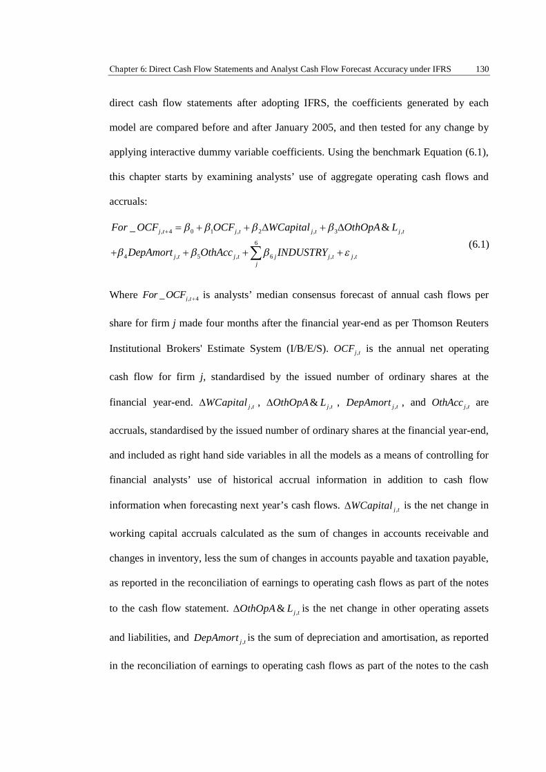
Chapter 6: Direct Cash Flow Statements and Analyst Cash Flow Forecast Accuracy under IFRS 130
direct cash flow statements after adopting IFRS, the coefficients generated by each
model are compared before and after January 2005, and then tested for any change by
applying interactive dummy variable coefficients. Using the benchmark Equation (6.1),
this chapter starts by examining analysts’ use of aggregate operating cash flows and
accruals:
, 4 0 1 , 2 , 3 ,
6
4 , 5 , 6 , ,
_ &
j t j t j t j t
j t j t j j t j tj
For OCF OCF WCapital OthOpA L
DepAmort OthAcc INDUSTRY(6.1)
Where , 4_ j tFor OCF is analysts’ median consensus forecast of annual cash flows per
share for firm j made four months after the financial year-end as per Thomson Reuters
Institutional Brokers' Estimate System (I/B/E/S). ,j tOCF is the annual net operating
cash flow for firm j, standardised by the issued number of ordinary shares at the
financial year-end. ,j tWCapital , ,& j tOthOpA L , ,j tDepAmort , and ,j tOthAcc are
accruals, standardised by the issued number of ordinary shares at the financial year-end,
and included as right hand side variables in all the models as a means of controlling for
financial analysts’ use of historical accrual information in addition to cash flow
information when forecasting next year’s cash flows. ,j tWCapital is the net change in
working capital accruals calculated as the sum of changes in accounts receivable and
changes in inventory, less the sum of changes in accounts payable and taxation payable,
as reported in the reconciliation of earnings to operating cash flows as part of the notes
to the cash flow statement. ,& j tOthOpA L is the net change in other operating assets
and liabilities, and ,j tDepAmort is the sum of depreciation and amortisation, as reported
in the reconciliation of earnings to operating cash flows as part of the notes to the cash
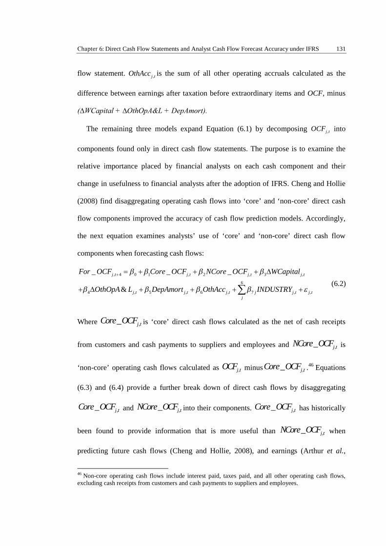
Chapter 6: Direct Cash Flow Statements and Analyst Cash Flow Forecast Accuracy under IFRS 131
flow statement. ,j tOthAcc is the sum of all other operating accruals calculated as the
difference between earnings after taxation before extraordinary items and OCF, minus
(∆WCapital + ∆OthOpA&L + DepAmort).
The remaining three models expand Equation (6.1) by decomposing ,j tOCF into
components found only in direct cash flow statements. The purpose is to examine the
relative importance placed by financial analysts on each cash component and their
change in usefulness to financial analysts after the adoption of IFRS. Cheng and Hollie
(2008) find disaggregating operating cash flows into ‘core’ and ‘non-core’ direct cash
flow components improved the accuracy of cash flow prediction models. Accordingly,
the next equation examines analysts’ use of ‘core’ and ‘non-core’ direct cash flow
components when forecasting cash flows:
, 4 0 1 , 2 , 3 ,
6
4 , 5 , 6 , 7 , ,
_ _ _
&
j t j t j t j t
j t j t j t j j t j tj
For OCF Core OCF NCore OCF WCapital
OthOpA L DepAmort OthAcc INDUSTRY(6.2)
Where ,_ j tCore OCF is ‘core’ direct cash flows calculated as the net of cash receipts
from customers and cash payments to suppliers and employees and ,_ j tNCore OCF is
‘non-core’ operating cash flows calculated as ,j tOCF minus ,_ j tCore OCF .46 Equations
(6.3) and (6.4) provide a further break down of direct cash flows by disaggregating
,_ j tCore OCF and ,_ j tNCore OCF into their components. ,_ j tCore OCF has historically
been found to provide information that is more useful than ,_ j tNCore OCF when
predicting future cash flows (Cheng and Hollie, 2008), and earnings (Arthur et al.,
46 Non-core operating cash flows include interest paid, taxes paid, and all other operating cash flows,excluding cash receipts from customers and cash payments to suppliers and employees.
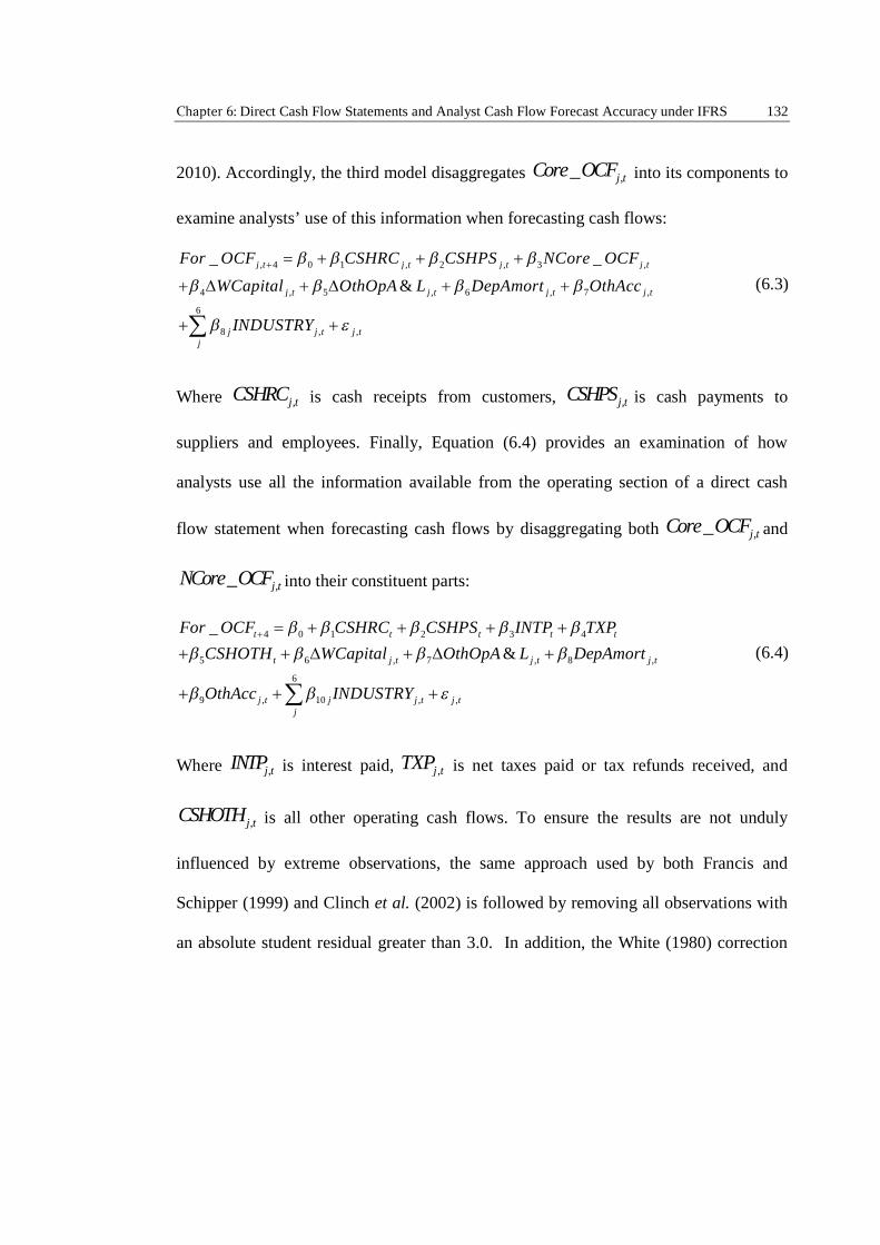
Chapter 6: Direct Cash Flow Statements and Analyst Cash Flow Forecast Accuracy under IFRS 132
2010). Accordingly, the third model disaggregates ,_ j tCore OCF into its components to
examine analysts’ use of this information when forecasting cash flows:
, 4 0 1 , 2 , 3 ,
4 , 5 , 6 , 7 ,
6
8 , ,
_ _
&
j t j t j t j t
j t j t j t j t
j j t j tj
For OCF CSHRC CSHPS NCore OCF
WCapital OthOpA L DepAmort OthAcc
INDUSTRY
(6.3)
Where ,j tCSHRC is cash receipts from customers, ,j tCSHPS is cash payments to
suppliers and employees. Finally, Equation (6.4) provides an examination of how
analysts use all the information available from the operating section of a direct cash
flow statement when forecasting cash flows by disaggregating both ,_ j tCore OCF and
,_ j tNCore OCF into their constituent parts:
4 0 1 2 3 4
5 6 , 7 , 8 ,
6
9 , 10 , ,
_
&
t t t t t
t j t j t j t
j t j j t j tj
For OCF CSHRC CSHPS INTP TXP
CSHOTH WCapital OthOpA L DepAmort
OthAcc INDUSTRY
(6.4)
Where ,j tINTP is interest paid, ,j tTXP is net taxes paid or tax refunds received, and
,j tCSHOTH is all other operating cash flows. To ensure the results are not unduly
influenced by extreme observations, the same approach used by both Francis and
Schipper (1999) and Clinch et al. (2002) is followed by removing all observations with
an absolute student residual greater than 3.0. In addition, the White (1980) correction
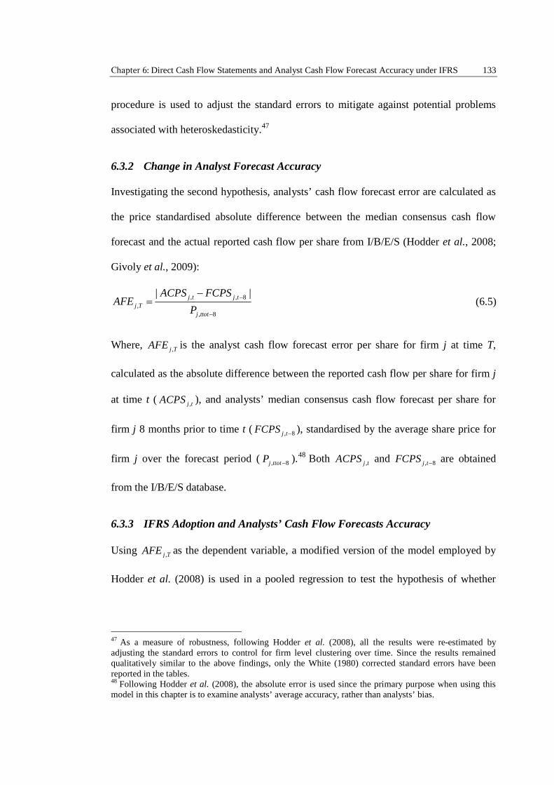
Chapter 6: Direct Cash Flow Statements and Analyst Cash Flow Forecast Accuracy under IFRS 133
procedure is used to adjust the standard errors to mitigate against potential problems
associated with heteroskedasticity.47
6.3.2 Change in Analyst Forecast Accuracy
Investigating the second hypothesis, analysts’ cash flow forecast error are calculated as
the price standardised absolute difference between the median consensus cash flow
forecast and the actual reported cash flow per share from I/B/E/S (Hodder et al., 2008;
Givoly et al., 2009):
, , 8
,
, 8
| |
j t j t
j T
j ttot
ACPS FCPSAFE
P(6.5)
Where, ,j TAFE is the analyst cash flow forecast error per share for firm j at time T,
calculated as the absolute difference between the reported cash flow per share for firm j
at time t ( ,j tACPS ), and analysts’ median consensus cash flow forecast per share for
firm j 8 months prior to time t ( , 8j tFCPS ), standardised by the average share price for
firm j over the forecast period ( , 8j ttotP ).48 Both ,j tACPS and , 8j tFCPS are obtained
from the I/B/E/S database.
6.3.3 IFRS Adoption and Analysts’ Cash Flow Forecasts Accuracy
Using ,j TAFE as the dependent variable, a modified version of the model employed by
Hodder et al. (2008) is used in a pooled regression to test the hypothesis of whether
47 As a measure of robustness, following Hodder et al. (2008), all the results were re-estimated byadjusting the standard errors to control for firm level clustering over time. Since the results remainedqualitatively similar to the above findings, only the White (1980) corrected standard errors have beenreported in the tables.48 Following Hodder et al. (2008), the absolute error is used since the primary purpose when using thismodel in this chapter is to examine analysts’ average accuracy, rather than analysts’ bias.
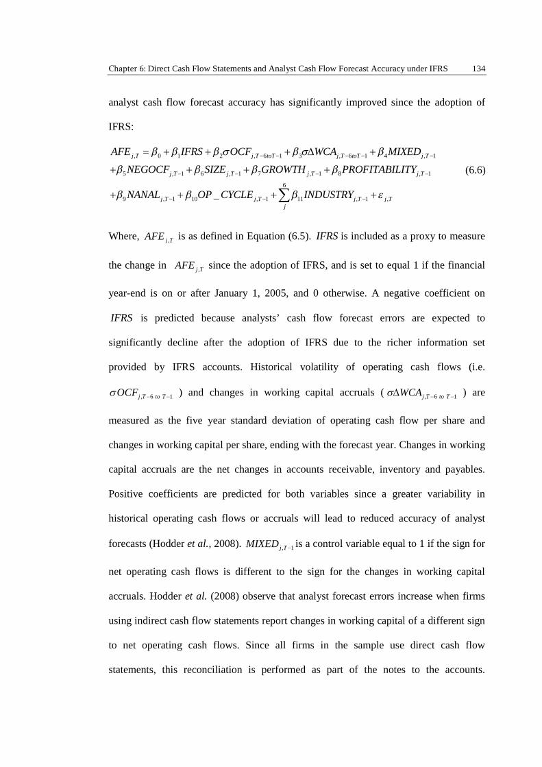
Chapter 6: Direct Cash Flow Statements and Analyst Cash Flow Forecast Accuracy under IFRS 134
analyst cash flow forecast accuracy has significantly improved since the adoption of
IFRS:
, 0 1 2 , 6 1 3 , 6 1 4 , 1
5 , 1 6 , 1 7 , 1 8 , 1
6
9 , 1 10 , 1 11 , 1 ,_
j T j T toT j T toT j T
j T j T j T j T
j T j T j T j Tj
AFE IFRS OCF WCA MIXED
NEGOCF SIZE GROWTH PROFITABILITY
NANAL OP CYCLE INDUSTRY
(6.6)
Where, ,j TAFE is as defined in Equation (6.5). IFRS is included as a proxy to measure
the change in ,j TAFE since the adoption of IFRS, and is set to equal 1 if the financial
year-end is on or after January 1, 2005, and 0 otherwise. A negative coefficient on
IFRS is predicted because analysts’ cash flow forecast errors are expected to
significantly decline after the adoption of IFRS due to the richer information set
provided by IFRS accounts. Historical volatility of operating cash flows (i.e.
, 6 1 j T to TOCF ) and changes in working capital accruals ( , 6 1 j T to TWCA ) are
measured as the five year standard deviation of operating cash flow per share and
changes in working capital per share, ending with the forecast year. Changes in working
capital accruals are the net changes in accounts receivable, inventory and payables.
Positive coefficients are predicted for both variables since a greater variability in
historical operating cash flows or accruals will lead to reduced accuracy of analyst
forecasts (Hodder et al., 2008). , 1j TMIXED is a control variable equal to 1 if the sign for
net operating cash flows is different to the sign for the changes in working capital
accruals. Hodder et al. (2008) observe that analyst forecast errors increase when firms
using indirect cash flow statements report changes in working capital of a different sign
to net operating cash flows. Since all firms in the sample use direct cash flow
statements, this reconciliation is performed as part of the notes to the accounts.
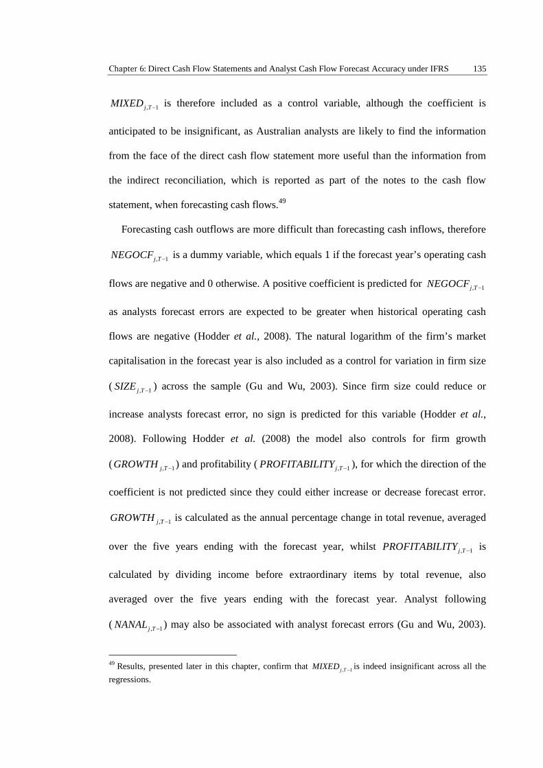
Chapter 6: Direct Cash Flow Statements and Analyst Cash Flow Forecast Accuracy under IFRS 135
, 1j TMIXED is therefore included as a control variable, although the coefficient is
anticipated to be insignificant, as Australian analysts are likely to find the information
from the face of the direct cash flow statement more useful than the information from
the indirect reconciliation, which is reported as part of the notes to the cash flow
statement, when forecasting cash flows.49
Forecasting cash outflows are more difficult than forecasting cash inflows, therefore
, 1j TNEGOCF is a dummy variable, which equals 1 if the forecast year’s operating cash
flows are negative and 0 otherwise. A positive coefficient is predicted for , 1j TNEGOCF
as analysts forecast errors are expected to be greater when historical operating cash
flows are negative (Hodder et al., 2008). The natural logarithm of the firm’s market
capitalisation in the forecast year is also included as a control for variation in firm size
( , 1j TSIZE ) across the sample (Gu and Wu, 2003). Since firm size could reduce or
increase analysts forecast error, no sign is predicted for this variable (Hodder et al.,
2008). Following Hodder et al. (2008) the model also controls for firm growth
( , 1j TGROWTH ) and profitability ( , 1j TPROFITABILITY ), for which the direction of the
coefficient is not predicted since they could either increase or decrease forecast error.
, 1j TGROWTH is calculated as the annual percentage change in total revenue, averaged
over the five years ending with the forecast year, whilst , 1j TPROFITABILITY is
calculated by dividing income before extraordinary items by total revenue, also
averaged over the five years ending with the forecast year. Analyst following
( , 1j TNANAL ) may also be associated with analyst forecast errors (Gu and Wu, 2003).
49 Results, presented later in this chapter, confirm that , 1j TMIXED is indeed insignificant across all the
regressions.
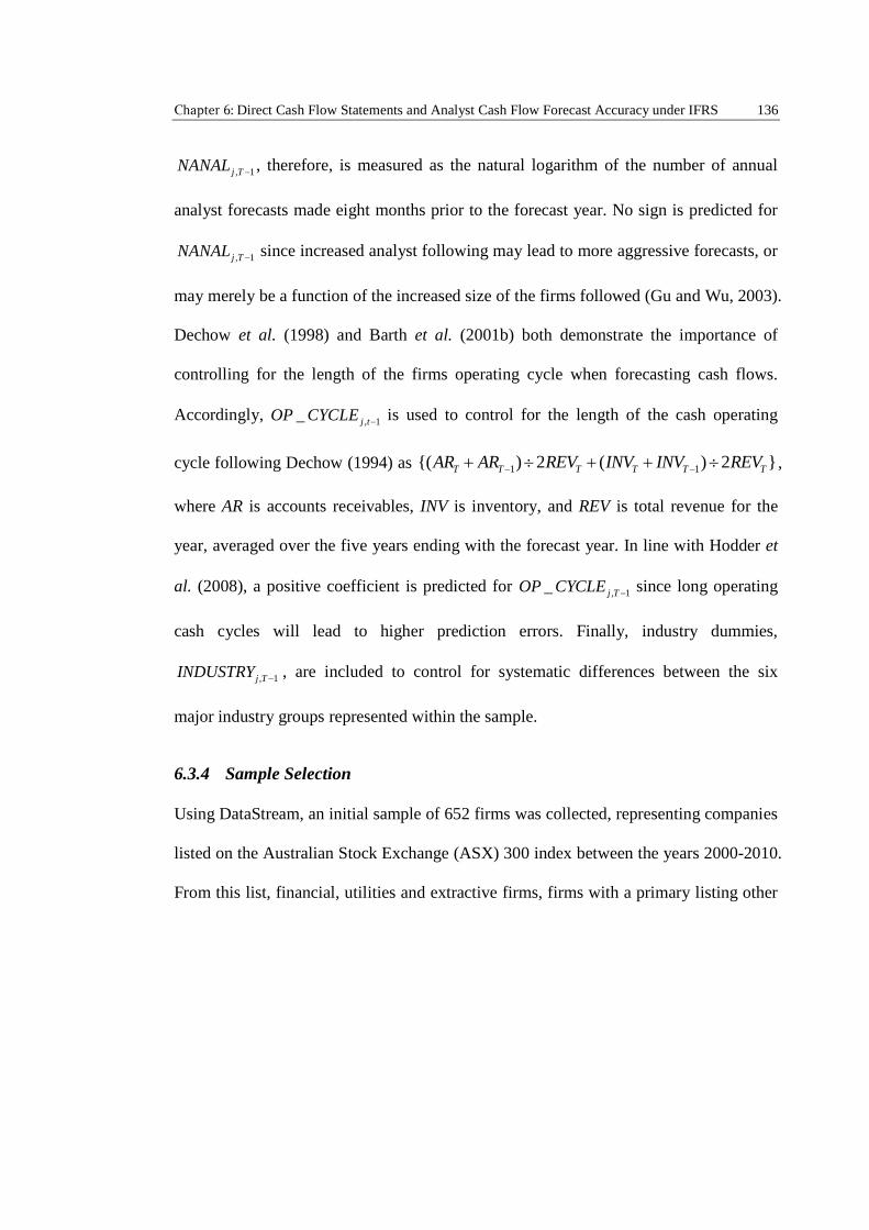
Chapter 6: Direct Cash Flow Statements and Analyst Cash Flow Forecast Accuracy under IFRS 136
, 1j TNANAL , therefore, is measured as the natural logarithm of the number of annual
analyst forecasts made eight months prior to the forecast year. No sign is predicted for
, 1j TNANAL since increased analyst following may lead to more aggressive forecasts, or
may merely be a function of the increased size of the firms followed (Gu and Wu, 2003).
Dechow et al. (1998) and Barth et al. (2001b) both demonstrate the importance of
controlling for the length of the firms operating cycle when forecasting cash flows.
Accordingly, , 1_ j tOP CYCLE is used to control for the length of the cash operating
cycle following Dechow (1994) as 1 1{( ) 2 ( ) 2 } T T T T T TAR AR REV INV INV REV ,
where AR is accounts receivables, INV is inventory, and REV is total revenue for the
year, averaged over the five years ending with the forecast year. In line with Hodder et
al. (2008), a positive coefficient is predicted for , 1_ j TOP CYCLE since long operating
cash cycles will lead to higher prediction errors. Finally, industry dummies,
, 1j TINDUSTRY , are included to control for systematic differences between the six
major industry groups represented within the sample.
6.3.4 Sample Selection
Using DataStream, an initial sample of 652 firms was collected, representing companies
listed on the Australian Stock Exchange (ASX) 300 index between the years 2000-2010.
From this list, financial, utilities and extractive firms, firms with a primary listing other
Chapter 6: Direct Cash Flow Statements and Analyst Cash Flow Forecast Accuracy under IFRS 137
than the ASX, and firms missing key financial information are removed.50 Further, all
firms are removed that subsequently chose to report their cash flows under the indirect
method. 51 From this sample a further 82 firms are removed due to missing or
incomplete analyst data from Thomson Reuters I/B/E/S.52 Next, all firms are removed
that have less than three analysts following them during the sample period. Finally, 93
firms are removed due to missing forecasts in either of the two years before or two
years after IFRS adoption. The final sample of 78 firms is shown in Table 6-1 Panel A.
Financial data used for the final sample of firms was obtained from the Aspect Huntley
database, which provides a detailed breakdown of the direct cash flows that are
otherwise unavailable elsewhere.
Table 6-1, Panel B, presents the distribution of the sample by industry classification
and firm-year across the sample period of eleven years from 2000-2010. It reveals that
firm numbers in all industry groups reach their peak around the transition of IFRS
between 2004 and 2005 due to the restriction placed on the sample that firms should
have forecasts in either of the two years before and two years after IFRS adoption. The
sample is dominated by two industry groups, consumer goods and services and
industrials, which, when combined, comprise 77% of firms.
50 Financial and utility firms are removed because of their different reporting requirements and foreigndomiciled firms are excluded, as they do not follow Australian GAAP. Of the few studies examining theusefulness of direct cash flows in Australia, Clinch et al.(2002) specifically treat mining firms separatelyfor their analysis whilst Arthur et al. (2010) exclude such firms. Extractive firms are excluded foranalysis in this chapter due to their unique line of business, which is often characterised by long periodsof cash outflow with little or no cash inflow. Furthermore, the lack of I/B/E/S data for extractive firms(only 12 extractive firms met the minimum data requirements) did not allow them to be treated separatelyfor analysis within this chapter.51 Australian firms were first permitted a choice between reporting their operating cash flows using thedirect or indirect method in April 2007 when the AASB amended AASB 107 by issuing AASBAmendment Pronouncement (AP) 2007-4.52 Examples include missing cash flow forecasts, missing number of analyst following, and missingactual cash flow per share per I/B/E/S.
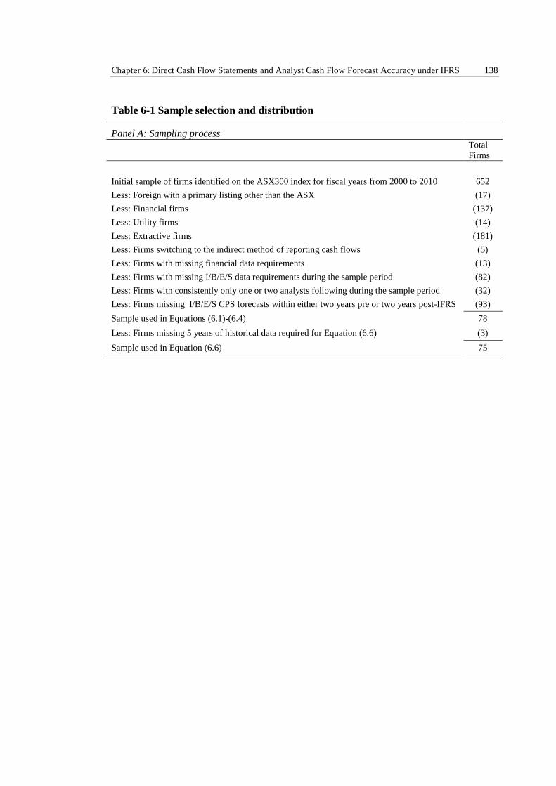
Chapter 6: Direct Cash Flow Statements and Analyst Cash Flow Forecast Accuracy under IFRS 138
Table 6-1 Sample selection and distribution
Panel A: Sampling processTotalFirms
Initial sample of firms identified on the ASX300 index for fiscal years from 2000 to 2010 652
Less: Foreign with a primary listing other than the ASX (17)
Less: Financial firms (137)
Less: Utility firms (14)
Less: Extractive firms (181)
Less: Firms switching to the indirect method of reporting cash flows (5)
Less: Firms with missing financial data requirements (13)
Less: Firms with missing I/B/E/S data requirements during the sample period (82)
Less: Firms with consistently only one or two analysts following during the sample period (32)
Less: Firms missing I/B/E/S CPS forecasts within either two years pre or two years post-IFRS (93)
Sample used in Equations (6.1)-(6.4) 78
Less: Firms missing 5 years of historical data required for Equation (6.6) (3)
Sample used in Equation (6.6) 75
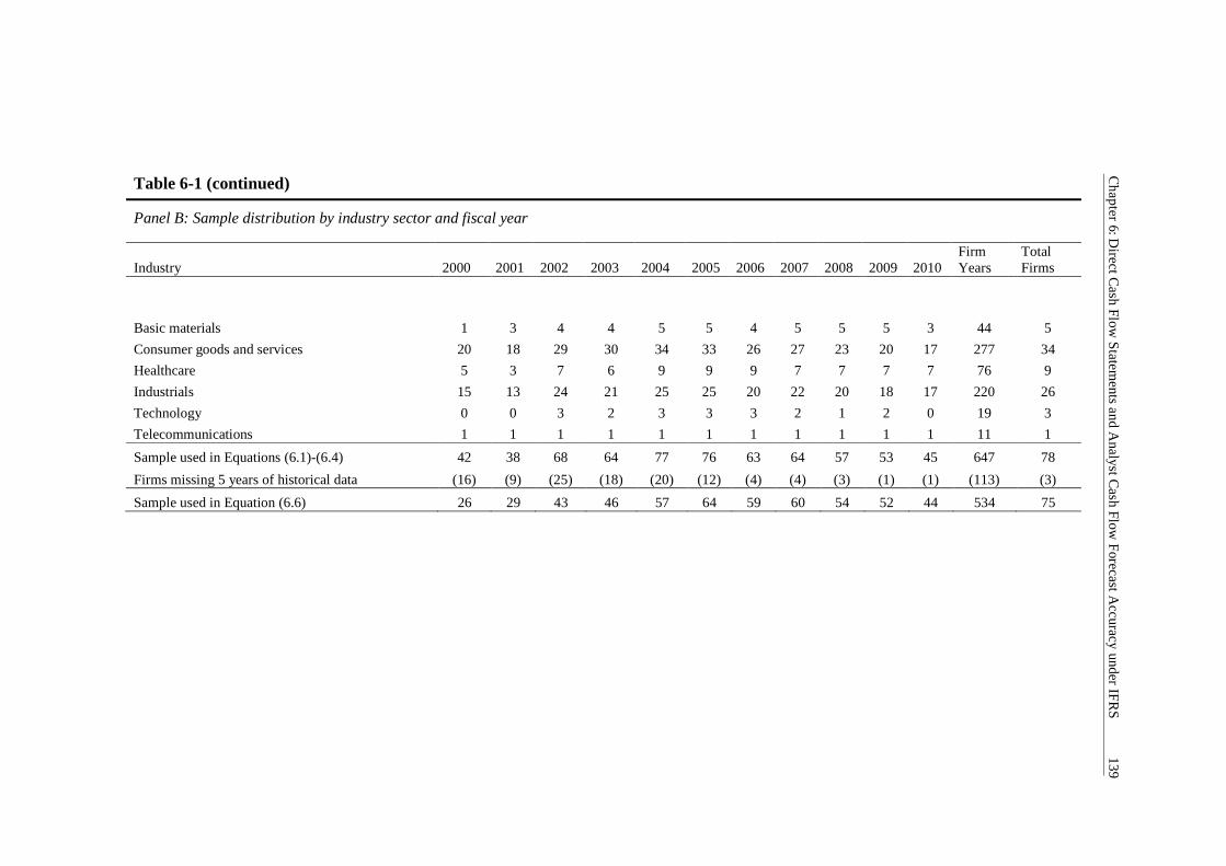
Ch
apter
6:Direct
Cash
Flow
Statem
entsan
dA
nalystC
ashF
lowF
orecastA
ccuracyunder
IFR
S13
9
Table 6-1 (continued)
Panel B: Sample distribution by industry sector and fiscal year
Industry 2000 2001 2002 2003 2004 2005 2006 2007 2008 2009 2010FirmYears
TotalFirms
Basic materials 1 3 4 4 5 5 4 5 5 5 3 44 5
Consumer goods and services 20 18 29 30 34 33 26 27 23 20 17 277 34
Healthcare 5 3 7 6 9 9 9 7 7 7 7 76 9
Industrials 15 13 24 21 25 25 20 22 20 18 17 220 26
Technology 0 0 3 2 3 3 3 2 1 2 0 19 3
Telecommunications 1 1 1 1 1 1 1 1 1 1 1 11 1
Sample used in Equations (6.1)-(6.4) 42 38 68 64 77 76 63 64 57 53 45 647 78
Firms missing 5 years of historical data (16) (9) (25) (18) (20) (12) (4) (4) (3) (1) (1) (113) (3)
Sample used in Equation (6.6) 26 29 43 46 57 64 59 60 54 52 44 534 75
Chapter 6: Direct Cash Flow Statements and Analyst Cash Flow Forecast Accuracy under IFRS 140
6.4 Results
6.4.1 Descriptive Statistics of Variables Used in Equations (6.1) to (6.4)
Table 6-2 provides descriptive statistics and correlation matrix for the key variables
used to investigate analysts’ use of direct cash flow components when preparing their
annual cash flow predictions. Further, this sample is also used to examine the change in
usefulness of direct cash flow components by analysts preparing annual cash flow
predictions since the adoption of IFRS. Table 6-2, Panel A, presents the descriptive
statistics for analysts’ median consensus annual cash flow forecast per share (For_OCF)
issued four months after the financial year-end as per I/B/E/S. Further, it provides
descriptive statistics of the direct cash flow components found in the operating section
of a direct cash flow statement. These include cash receipts from customers (CSHRC),
cash payments to suppliers and employees (CSHPS), interest paid (INTP), net taxes paid
(TXP), and the net of all other operating cash flows (CSHOTH), which, when all
aggregated, sum up to net operating cash flows (OCF). Table 6-2, Panel A, further
provides descriptive statistics for both ‘core’ (Core_OCF) and ‘non-core’ (NCore_OCF)
direct cash flows, defined as the net of CSHRC and CSHPS, and the difference between
OCF and Core_OCF respectively. Finally, statistics for the changes in working capital
accruals (ΔWCapital), changes in other operating assets and liabilities (ΔOthOpA&L),
depreciation and amortisation (DepAmort), and other operating accruals (OthAcc) are
included. All variables are deflated by the issued number of ordinary shares at the
financial year-end.
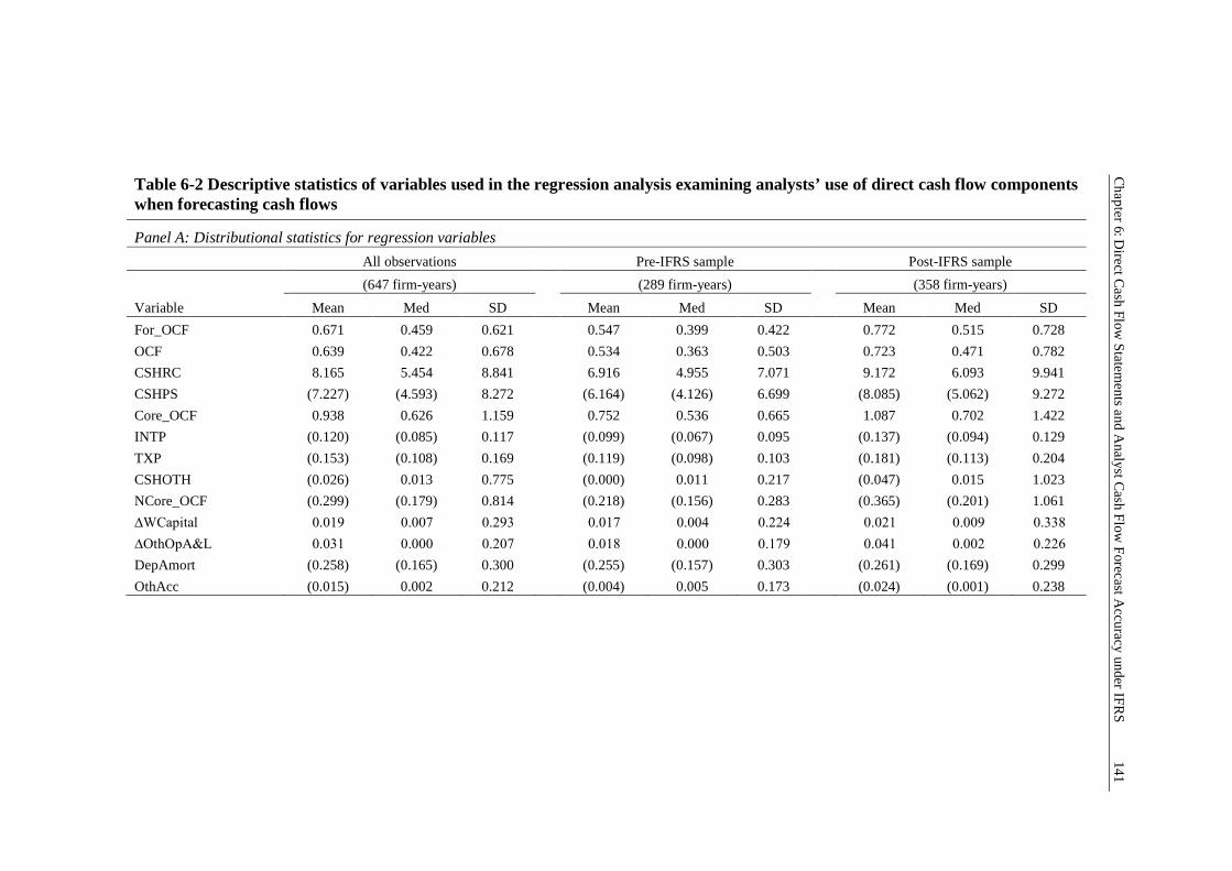
Ch
apter
6:Direct
Cash
Flow
Statem
entsan
dA
nalystC
ashF
lowF
orecastA
ccuracyunder
IFR
S14
1
Table 6-2 Descriptive statistics of variables used in the regression analysis examining analysts’ use of direct cash flow componentswhen forecasting cash flows
Panel A: Distributional statistics for regression variables
All observations Pre-IFRS sample Post-IFRS sample
(647 firm-years) (289 firm-years) (358 firm-years)
Variable Mean Med SD Mean Med SD Mean Med SD
For_OCF 0.671 0.459 0.621 0.547 0.399 0.422 0.772 0.515 0.728
OCF 0.639 0.422 0.678 0.534 0.363 0.503 0.723 0.471 0.782
CSHRC 8.165 5.454 8.841 6.916 4.955 7.071 9.172 6.093 9.941
CSHPS (7.227) (4.593) 8.272 (6.164) (4.126) 6.699 (8.085) (5.062) 9.272
Core_OCF 0.938 0.626 1.159 0.752 0.536 0.665 1.087 0.702 1.422
INTP (0.120) (0.085) 0.117 (0.099) (0.067) 0.095 (0.137) (0.094) 0.129
TXP (0.153) (0.108) 0.169 (0.119) (0.098) 0.103 (0.181) (0.113) 0.204
CSHOTH (0.026) 0.013 0.775 (0.000) 0.011 0.217 (0.047) 0.015 1.023
NCore_OCF (0.299) (0.179) 0.814 (0.218) (0.156) 0.283 (0.365) (0.201) 1.061
∆WCapital 0.019 0.007 0.293 0.017 0.004 0.224 0.021 0.009 0.338
∆OthOpA&L 0.031 0.000 0.207 0.018 0.000 0.179 0.041 0.002 0.226
DepAmort (0.258) (0.165) 0.300 (0.255) (0.157) 0.303 (0.261) (0.169) 0.299
OthAcc (0.015) 0.002 0.212 (0.004) 0.005 0.173 (0.024) (0.001) 0.238
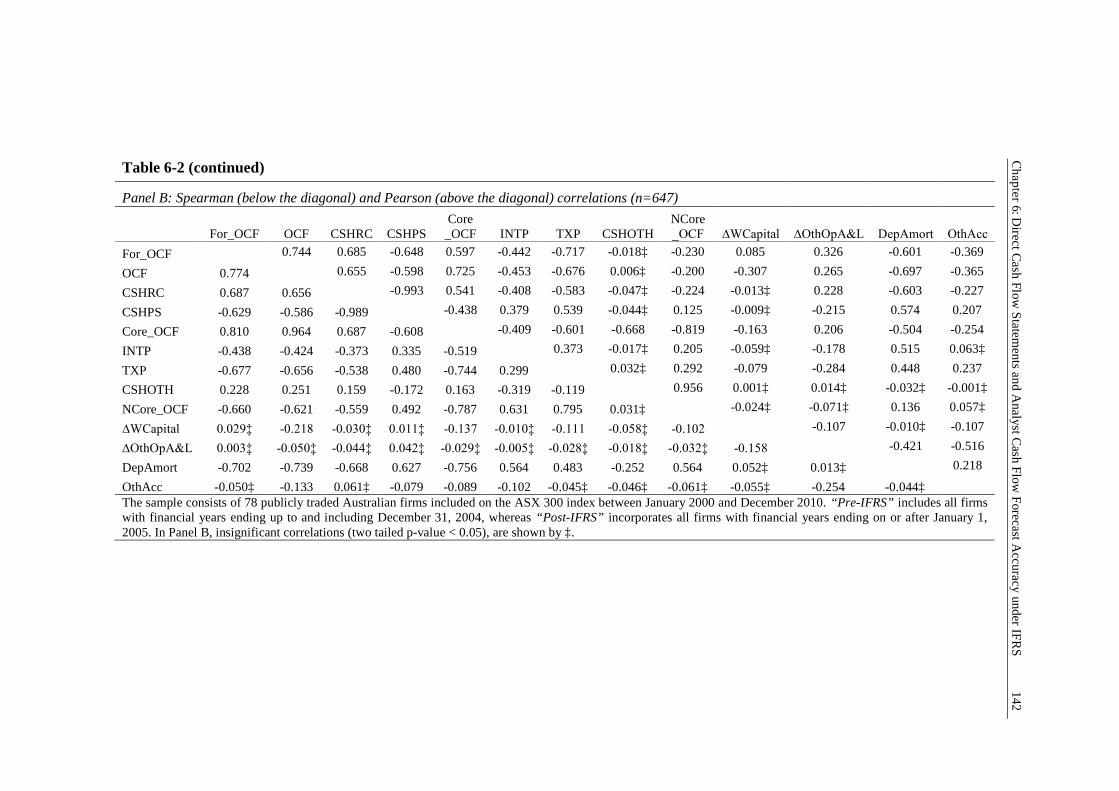
Ch
apter
6:Direct
Cash
Flow
Statem
entsan
dA
nalystC
ashF
lowF
orecastA
ccuracyunder
IFR
S14
2
Table 6-2 (continued)
Panel B: Spearman (below the diagonal) and Pearson (above the diagonal) correlations (n=647)
For_OCF OCF CSHRC CSHPSCore_OCF INTP TXP CSHOTH
NCore_OCF ∆WCapital ∆OthOpA&L DepAmort OthAcc
For_OCF 0.744 0.685 -0.648 0.597 -0.442 -0.717 -0.018‡ -0.230 0.085 0.326 -0.601 -0.369
OCF 0.774 0.655 -0.598 0.725 -0.453 -0.676 0.006‡ -0.200 -0.307 0.265 -0.697 -0.365
CSHRC 0.687 0.656 -0.993 0.541 -0.408 -0.583 -0.047‡ -0.224 -0.013‡ 0.228 -0.603 -0.227
CSHPS -0.629 -0.586 -0.989 -0.438 0.379 0.539 -0.044‡ 0.125 -0.009‡ -0.215 0.574 0.207
Core_OCF 0.810 0.964 0.687 -0.608 -0.409 -0.601 -0.668 -0.819 -0.163 0.206 -0.504 -0.254
INTP -0.438 -0.424 -0.373 0.335 -0.519 0.373 -0.017‡ 0.205 -0.059‡ -0.178 0.515 0.063‡
TXP -0.677 -0.656 -0.538 0.480 -0.744 0.299 0.032‡ 0.292 -0.079 -0.284 0.448 0.237
CSHOTH 0.228 0.251 0.159 -0.172 0.163 -0.319 -0.119 0.956 0.001‡ 0.014‡ -0.032‡ -0.001‡
NCore_OCF -0.660 -0.621 -0.559 0.492 -0.787 0.631 0.795 0.031‡ -0.024‡ -0.071‡ 0.136 0.057‡
∆WCapital 0.029‡ -0.218 -0.030‡ 0.011‡ -0.137 -0.010‡ -0.111 -0.058‡ -0.102 -0.107 -0.010‡ -0.107
∆OthOpA&L 0.003‡ -0.050‡ -0.044‡ 0.042‡ -0.029‡ -0.005‡ -0.028‡ -0.018‡ -0.032‡ -0.158 -0.421 -0.516
DepAmort -0.702 -0.739 -0.668 0.627 -0.756 0.564 0.483 -0.252 0.564 0.052‡ 0.013‡ 0.218
OthAcc -0.050‡ -0.133 0.061‡ -0.079 -0.089 -0.102 -0.045‡ -0.046‡ -0.061‡ -0.055‡ -0.254 -0.044‡The sample consists of 78 publicly traded Australian firms included on the ASX 300 index between January 2000 and December 2010. “Pre-IFRS” includes all firmswith financial years ending up to and including December 31, 2004, whereas “Post-IFRS” incorporates all firms with financial years ending on or after January 1,2005. In Panel B, insignificant correlations (two tailed p-value < 0.05), are shown by ‡.
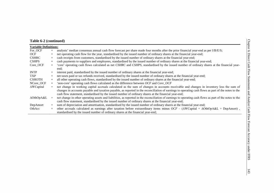
Ch
apter
6:Direct
Cash
Flow
Statem
entsan
dA
nalystC
ashF
lowF
orecastA
ccuracyunder
IFR
S14
3
Table 6-2 (continued)
Variable Definitions:For_OCF = analysts’ median consensus annual cash flow forecast per share made four months after the prior financial year-end as per I/B/E/S;OCF = net operating cash flow for the year, standardised by the issued number of ordinary shares at the financial year-end;CSHRC = cash receipts from customers, standardised by the issued number of ordinary shares at the financial year-end;CSHPS = cash payments to suppliers and employees, standardised by the issued number of ordinary shares at the financial year-end;Core_OCF = ‘core’ operating cash flows calculated as net CSHRC and CSHPS, standardised by the issued number of ordinary shares at the financial year-
end;INTP = interest paid, standardised by the issued number of ordinary shares at the financial year-end;TXP = net taxes paid or tax refunds received, standardised by the issued number of ordinary shares at the financial year-end;CSHOTH = all other operating cash flows, standardised by the issued number of ordinary shares at the financial year-end;NCore_OCF = ‘non-core’ operating cash flows calculated as the difference between OCF and Core_OCF∆WCapital = net change in working capital accruals calculated as the sum of changes in accounts receivable and changes in inventory less the sum of
changes in accounts payable and taxation payable, as reported in the reconciliation of earnings to operating cash flows as part of the notes to thecash flow statement, standardised by the issued number of ordinary shares at the financial year-end;
∆OthOpA&L = net change in other operating assets and liabilities, as reported in the reconciliation of earnings to operating cash flows as part of the notes to the cash flow statement, standardised by the issued number of ordinary shares at the financial year-end;
DepAmort = sum of depreciation and amortisation, standardised by the issued number of ordinary shares at the financial year-end;OthAcc = other accruals calculated as earnings after taxation before extraordinary items minus OCF – (∆WCapital + ∆OthOpA&L + DepAmort) ,
standardised by the issued number of ordinary shares at the financial year-end;
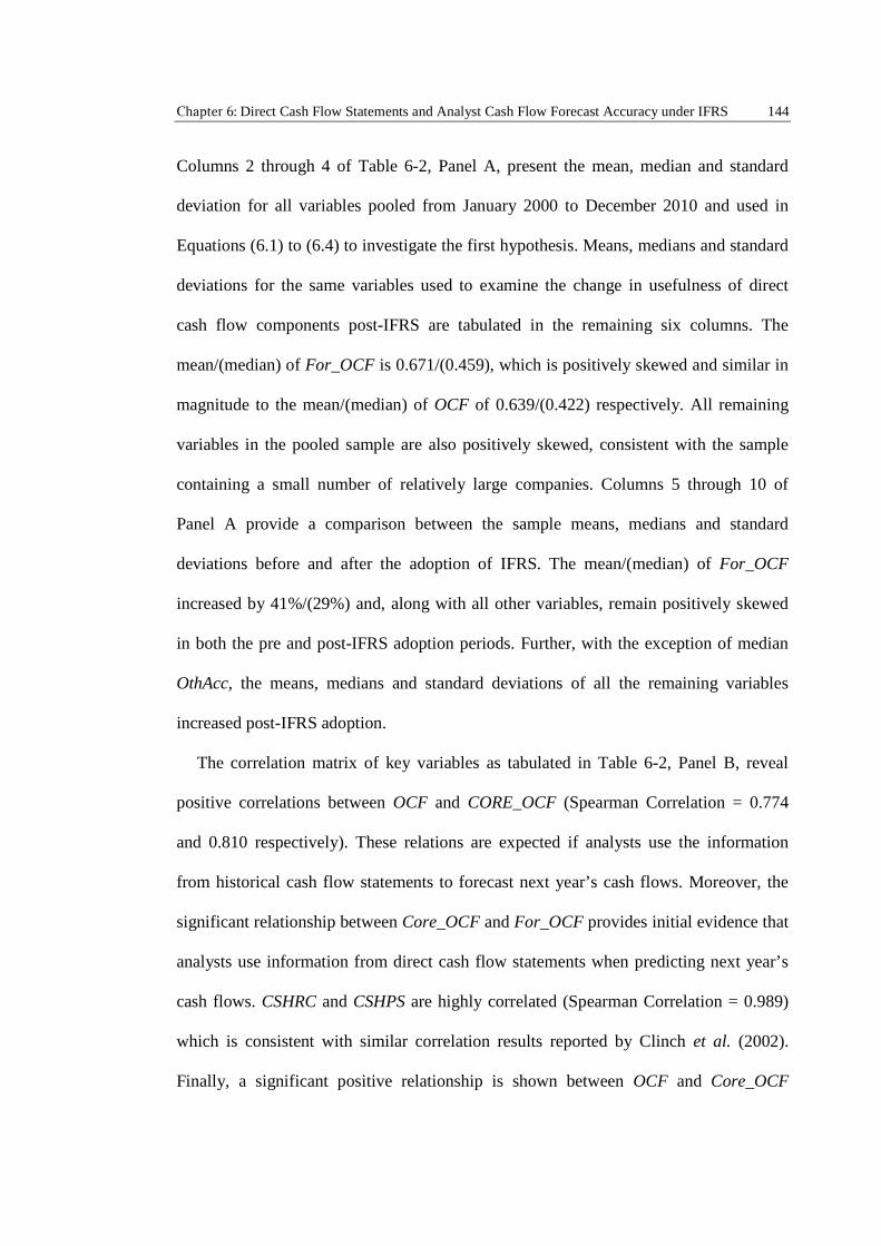
Chapter 6: Direct Cash Flow Statements and Analyst Cash Flow Forecast Accuracy under IFRS 144
Columns 2 through 4 of Table 6-2, Panel A, present the mean, median and standard
deviation for all variables pooled from January 2000 to December 2010 and used in
Equations (6.1) to (6.4) to investigate the first hypothesis. Means, medians and standard
deviations for the same variables used to examine the change in usefulness of direct
cash flow components post-IFRS are tabulated in the remaining six columns. The
mean/(median) of For_OCF is 0.671/(0.459), which is positively skewed and similar in
magnitude to the mean/(median) of OCF of 0.639/(0.422) respectively. All remaining
variables in the pooled sample are also positively skewed, consistent with the sample
containing a small number of relatively large companies. Columns 5 through 10 of
Panel A provide a comparison between the sample means, medians and standard
deviations before and after the adoption of IFRS. The mean/(median) of For_OCF
increased by 41%/(29%) and, along with all other variables, remain positively skewed
in both the pre and post-IFRS adoption periods. Further, with the exception of median
OthAcc, the means, medians and standard deviations of all the remaining variables
increased post-IFRS adoption.
The correlation matrix of key variables as tabulated in Table 6-2, Panel B, reveal
positive correlations between OCF and CORE_OCF (Spearman Correlation = 0.774
and 0.810 respectively). These relations are expected if analysts use the information
from historical cash flow statements to forecast next year’s cash flows. Moreover, the
significant relationship between Core_OCF and For_OCF provides initial evidence that
analysts use information from direct cash flow statements when predicting next year’s
cash flows. CSHRC and CSHPS are highly correlated (Spearman Correlation = 0.989)
which is consistent with similar correlation results reported by Clinch et al. (2002).
Finally, a significant positive relationship is shown between OCF and Core_OCF
Chapter 6: Direct Cash Flow Statements and Analyst Cash Flow Forecast Accuracy under IFRS 145
(Spearman Correlation = 0.964), providing further impetus to treat Core_OCF as a
separate explanatory variable in Equation (6.2).
6.4.2 Descriptive Statistics of Variables Used in Equation (6.6)
Table 6-3 presents the descriptive statistics for the sample used to investigate the
change in analysts’ cash flow forecast errors since the adoption of IFRS. Three firms
and 113 firm-year observations were excluded from the final sample presented in Table
6-1 due to the strict limitation imposed by calculating the five-year historical averages
and standard deviations for some of the key variables used in Equation (6.6). Columns 2
through 6 present the means, standard deviation, medians, and quartiles for the key
variables used in Equation (6.6). Pre and post-IFRS period medians and means for the
same variables are separately presented in columns 7 to 10, along with results from the
univariate tests examining the equality of means between both periods.
The mean absolute value of the analysts’ cash flow forecast error (AFE) standardised
by the average share price is 0.046, more than twice the median of 0.017, revealing a
large proportion of firms with relatively small forecast errors. These statistics are
consistent with those documented by Hodder et al. (2008) which report a mean/(median)
AFE of 0.036/(0.017) respectively for their sample of U.S. firms. With the exception of
the logarithmic number of analysts forecasting future cash flows (NANAL) of 1.781, the
remaining variables are all positively skewed. Historical operating cash flows (OCF)
are comparatively more volatile than changes in historical working capital accruals
(ΔWCA), evidenced by the higher average five-year standard deviation of 0.222 for
OCF compared to 0.181 for ΔWCA.
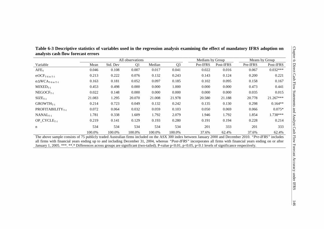
Ch
apter
6:Direct
Cash
Flow
Statem
entsan
dA
nalystC
ashF
lowF
orecastA
ccuracyunder
IFR
S14
6
Table 6-3 Descriptive statistics of variables used in the regression analysis examining the effect of mandatory IFRS adoption onanalysts cash flow forecast errors
All observations Medians by Group Means by Group
Variable Mean Std. Dev Q1 Median Q3 Pre-IFRS Post-IFRS Pre-IFRS Post-IFRS
AFET 0.046 0.108 0.007 0.017 0.041 0.022 0.016 0.067 0.032***
OCFT-6 to T-1 0.213 0.222 0.076 0.132 0.243 0.143 0.124 0.200 0.221
ΔWCAT-6 to T-1 0.163 0.181 0.052 0.097 0.185 0.102 0.095 0.158 0.167
MIXEDT-1 0.453 0.498 0.000 0.000 1.000 0.000 0.000 0.473 0.441
NEGOCFT-1 0.022 0.148 0.000 0.000 0.000 0.000 0.000 0.035 0.015
SIZET-1 21.083 1.295 20.070 21.008 21.978 20.580 21.188 20.778 21.267***
GROWTHT-1 0.214 0.723 0.049 0.132 0.242 0.135 0.130 0.298 0.164**
PROFITABILITYT-1 0.072 0.064 0.032 0.059 0.103 0.050 0.069 0.066 0.075*
NANALT-1 1.781 0.338 1.609 1.792 2.079 1.946 1.792 1.854 1.738***
OP_CYCLET-1 0.219 0.141 0.129 0.193 0.280 0.191 0.194 0.228 0.214
n 534 534 534 534 534 201 333 201 333
100.0% 100.0% 100.0% 100.0% 100.0% 37.6% 62.4% 37.6% 62.4%The above sample consists of 75 publicly traded Australian firms included on the ASX 300 index between January 2000 and December 2010. “Pre-IFRS” includesall firms with financial years ending up to and including December 31, 2004, whereas “Post-IFRS” incorporates all firms with financial years ending on or afterJanuary 1, 2005. ***. **.* Differences across groups are significant (two-tailed). P-value p<0.01, p<0.05, p<0.1 levels of significance respectively.
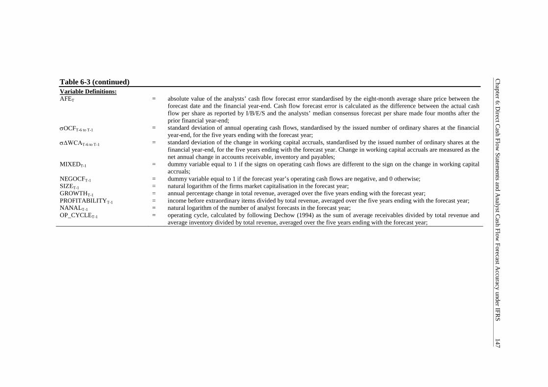
Ch
apter
6:Direct
Cash
Flow
Statem
entsan
dA
nalystC
ashF
lowF
orecastA
ccuracyunder
IFR
S14
7
Table 6-3 (continued)Variable Definitions:AFET = absolute value of the analysts’ cash flow forecast error standardised by the eight-month average share price between the
forecast date and the financial year-end. Cash flow forecast error is calculated as the difference between the actual cashflow per share as reported by I/B/E/S and the analysts’ median consensus forecast per share made four months after theprior financial year-end;
OCFT-6 to T-1 = standard deviation of annual operating cash flows, standardised by the issued number of ordinary shares at the financialyear-end, for the five years ending with the forecast year;
ΔWCAT-6 to T-1 = standard deviation of the change in working capital accruals, standardised by the issued number of ordinary shares at thefinancial year-end, for the five years ending with the forecast year. Change in working capital accruals are measured as thenet annual change in accounts receivable, inventory and payables;
MIXEDT-1 = dummy variable equal to 1 if the signs on operating cash flows are different to the sign on the change in working capitalaccruals;
NEGOCFT-1 = dummy variable equal to 1 if the forecast year’s operating cash flows are negative, and 0 otherwise;SIZET-1 = natural logarithm of the firms market capitalisation in the forecast year;GROWTHT-1 = annual percentage change in total revenue, averaged over the five years ending with the forecast year;PROFITABILITYT-1 = income before extraordinary items divided by total revenue, averaged over the five years ending with the forecast year;NANALT-1 = natural logarithm of the number of analyst forecasts in the forecast year;OP_CYCLET-1 = operating cycle, calculated by following Dechow (1994) as the sum of average receivables divided by total revenue and
average inventory divided by total revenue, averaged over the five years ending with the forecast year;
Chapter 6: Direct Cash Flow Statements and Analyst Cash Flow Forecast Accuracy under IFRS 148
Approximately 45% of firms reveal mixed signs between OCF and ΔWCA, while
only 2% of firms report negative operating cash flows. This is likely because the sample
only includes firms that were historically represented in the 300 largest firms in
Australia where reporting negative operating cash flows would be uncommon. Hence,
the average firm size of 21.083, calculated as the logarithm of market capitalisation, is
relatively larger than the 8.213 value reported from the wider U.S. sample used by
Hodder et al. (2008). Five-year average revenue growth, profitability, and operating
cycle over the eleven-year period were approximately 21%, 7%, and 80 days
respectively.
Univariate tests of comparisons between the pre and post-IFRS periods reveal some
significant changes in the means for a number of the key variables. Specifically, a 52%
decline is observed in the mean absolute value of analysts cash flow forecast error to
0.032 post-IFRS, providing initial evidence that the accuracy of cash flow forecasts
significantly improved subsequent to the adoption of IFRS. The mean logarithm of
market capitalisation increased by more than 2%, which univariate tests indicate is a
significant growth in firm size post-IFRS. However, mean revenue growth nearly
halved from 30% to 16%, a decline of 47%. On average firms were marginally more
profitable post-IFRS, reporting a net profit margin of 7.5%, up 14% from 6.6% in the
pre-IFRS period. There was also a significant fall in the average number of analysts
issuing annual cash flow forecasts post-IFRS. Finally, a comparison between the
medians and means in columns 7 to 10 reveal that all variables, with the exception of
NANAL, remain positively skewed both before and after IFRS.
Chapter 6: Direct Cash Flow Statements and Analyst Cash Flow Forecast Accuracy under IFRS 149
6.4.3 IFRS Adoption and Analysts’ Use of Direct Cash Flow Components
Investigating the first hypotheses, Table 6-4 to 6-7 summarise the results for estimating
Equations (6.1) to (6.4) on a pooled basis, before and after the adoption of IFRS in
Australia. All variables are analysed on a per share basis. The tables report mean
coefficients, two tailed t-statistics, and adjusted R2 values for the pooled sample (from
January 2000 to December 2010), pre-IFRS (from January 2000 to December 2004),
post-IFRS (from January 2005 to December 2010), and pre vs. post-IFRS respectively.
Results from columns 1 to 3 are used to test the first hypothesis of whether analysts find
information from direct cash flow statements useful when predicting future cash flows.
Interactive dummy variables used in column 4 of each table test whether analysts find
information from direct cash flow statements significantly more useful after adopting
IFRS.
6.4.3.1 Usefulness of Aggregate Historical Operating Cash Flows
Table 6-4 presents results from the benchmark Equation (6.1) by testing analysts’ use of
aggregate operating cash flows and accruals components, prior to disaggregating cash
flows into their components in the subsequent tables. The cash flow coefficients are
positive and significant in columns 1 to 3 providing evidence that analysts find
information regarding historical cash flows useful when predicting next year’s cash
flows, and this holds both before and after the adoption of IFRS. Columns 1 to 3 further
reveal ΔWCapital, ΔOthOpA&L, and OthAcc are also significant, while DepAmort is
significant for the pooled and pre-IFRS regressions only. These findings further justify
the inclusion of these accruals components as controls within each model since they
show analysts also find information regarding historical accrual components useful
when forecasting future cash flows.
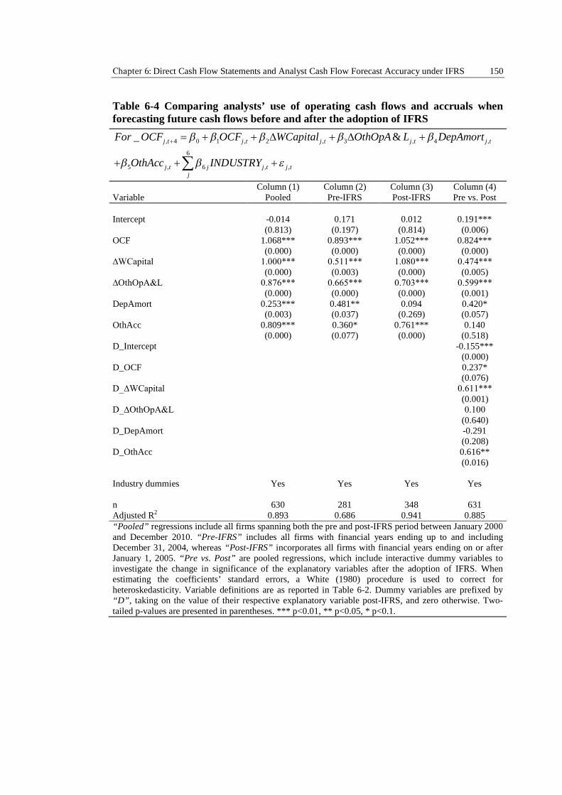
Chapter 6: Direct Cash Flow Statements and Analyst Cash Flow Forecast Accuracy under IFRS 150
Table 6-4 Comparing analysts’ use of operating cash flows and accruals whenforecasting future cash flows before and after the adoption of IFRS
, 4 0 1 , 2 , 3 , 4 ,
6
5 , 6 , ,
_ &
j t j t j t j t j t
j t j j t j tj
For OCF OCF WCapital OthOpA L DepAmort
OthAcc INDUSTRY
Column (1) Column (2) Column (3) Column (4)Variable Pooled Pre-IFRS Post-IFRS Pre vs. Post
Intercept -0.014 0.171 0.012 0.191***(0.813) (0.197) (0.814) (0.006)
OCF 1.068*** 0.893*** 1.052*** 0.824***(0.000) (0.000) (0.000) (0.000)
∆WCapital 1.000*** 0.511*** 1.080*** 0.474*** (0.000) (0.003) (0.000) (0.005)
∆OthOpA&L 0.876*** 0.665*** 0.703*** 0.599*** (0.000) (0.000) (0.000) (0.001)
DepAmort 0.253*** 0.481** 0.094 0.420*(0.003) (0.037) (0.269) (0.057)
OthAcc 0.809*** 0.360* 0.761*** 0.140(0.000) (0.077) (0.000) (0.518)
D_Intercept -0.155***(0.000)
D_OCF 0.237*(0.076)
D_∆WCapital 0.611*** (0.001)
D_∆OthOpA&L 0.100 (0.640)
D_DepAmort -0.291(0.208)
D_OthAcc 0.616**(0.016)
Industry dummies Yes Yes Yes Yes
n 630 281 348 631Adjusted R2 0.893 0.686 0.941 0.885“Pooled” regressions include all firms spanning both the pre and post-IFRS period between January 2000and December 2010. “Pre-IFRS” includes all firms with financial years ending up to and includingDecember 31, 2004, whereas “Post-IFRS” incorporates all firms with financial years ending on or afterJanuary 1, 2005. “Pre vs. Post” are pooled regressions, which include interactive dummy variables toinvestigate the change in significance of the explanatory variables after the adoption of IFRS. Whenestimating the coefficients’ standard errors, a White (1980) procedure is used to correct forheteroskedasticity. Variable definitions are as reported in Table 6-2. Dummy variables are prefixed by“D”, taking on the value of their respective explanatory variable post-IFRS, and zero otherwise. Two-tailed p-values are presented in parentheses. *** p<0.01, ** p<0.05, * p<0.1.
Chapter 6: Direct Cash Flow Statements and Analyst Cash Flow Forecast Accuracy under IFRS 151
The results from column 4 further show a significant positive mean coefficient for
ΔWCapital and OthAcc dummy variables of 0.611 and 0.616 respectively, a result that
remains consistent for Table 6-5 to 6-7. Further, operating cash flows are shown to
increase in usefulness, evidenced by the coefficient of 0.237 for the OCF dummy
variable, revealing financial analysts’ find historical operating cash flows, changes in
working capital accruals and other accruals more useful when forecasting future cash
flows under IFRS. In summary, historical operating cash flows, working capital
accruals and other accruals are not only used by financial analysts, but are significantly
more useful to financial analysts post-IFRS, when predicting next year’s cash flows.
6.4.3.2 Usefulness of ‘Core’ and ‘Non-core’ Direct Cash Flows
Following Cheng and Hollie (2008), OCF is disaggregated into ‘core’ (Core_OCF) and
‘non-core’ (NCore_OCF) direct cash flows in Equation (6.2), with the results reported
in Table 6-5. Consistent with H1, the mean coefficients for both Core_OCF and
NCore_OCF are positive and highly significant under local GAAP and IFRS, and
across the pooled sample period. Further, the mean coefficients for ΔWCapital and
OthAcc remain positive and highly significant under AGAAP and IFRS. Coefficients
for DepAmort are significant for the pooled regression and pre-IFRS, and the
coefficients for ΔOthOpA&L are significant post-IFRS and for the pooled regression.
Net cash receipts from customers and payments to suppliers and employees,
information only available from direct cash flow statements, is clearly useful to
financial analysts when predicting annual cash flows.
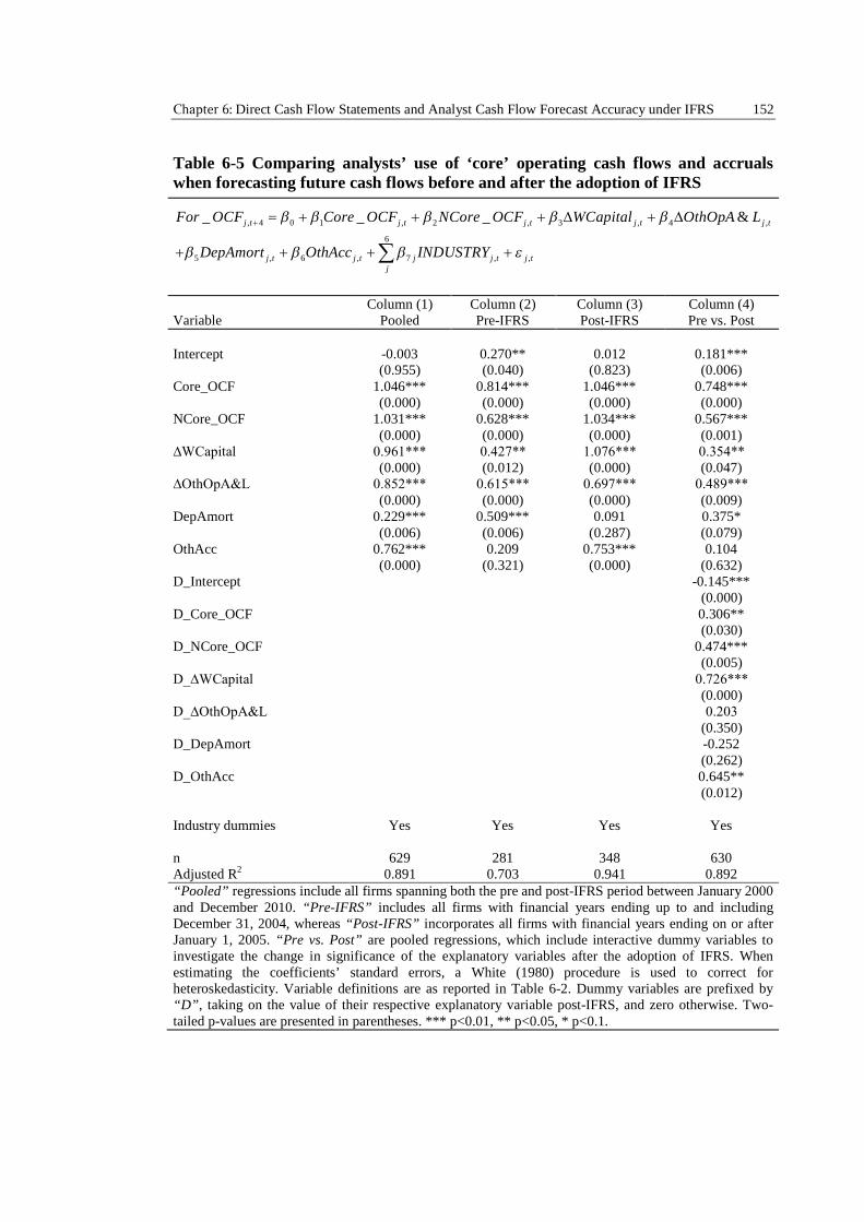
Chapter 6: Direct Cash Flow Statements and Analyst Cash Flow Forecast Accuracy under IFRS 152
Table 6-5 Comparing analysts’ use of ‘core’ operating cash flows and accrualswhen forecasting future cash flows before and after the adoption of IFRS
, 4 0 1 , 2 , 3 , 4 ,
6
5 , 6 , 7 , ,
_ _ _ &
j t j t j t j t j t
j t j t j j t j tj
For OCF Core OCF NCore OCF WCapital OthOpA L
DepAmort OthAcc INDUSTRY
Column (1) Column (2) Column (3) Column (4)Variable Pooled Pre-IFRS Post-IFRS Pre vs. Post
Intercept -0.003 0.270** 0.012 0.181***(0.955) (0.040) (0.823) (0.006)
Core_OCF 1.046*** 0.814*** 1.046*** 0.748***(0.000) (0.000) (0.000) (0.000)
NCore_OCF 1.031*** 0.628*** 1.034*** 0.567***(0.000) (0.000) (0.000) (0.001)
∆WCapital 0.961*** 0.427** 1.076*** 0.354** (0.000) (0.012) (0.000) (0.047)
∆OthOpA&L 0.852*** 0.615*** 0.697*** 0.489*** (0.000) (0.000) (0.000) (0.009)
DepAmort 0.229*** 0.509*** 0.091 0.375*(0.006) (0.006) (0.287) (0.079)
OthAcc 0.762*** 0.209 0.753*** 0.104(0.000) (0.321) (0.000) (0.632)
D_Intercept -0.145***(0.000)
D_Core_OCF 0.306**(0.030)
D_NCore_OCF 0.474***(0.005)
D_∆WCapital 0.726*** (0.000)
D_∆OthOpA&L 0.203 (0.350)
D_DepAmort -0.252(0.262)
D_OthAcc 0.645**(0.012)
Industry dummies Yes Yes Yes Yes
n 629 281 348 630Adjusted R2 0.891 0.703 0.941 0.892“Pooled” regressions include all firms spanning both the pre and post-IFRS period between January 2000and December 2010. “Pre-IFRS” includes all firms with financial years ending up to and includingDecember 31, 2004, whereas “Post-IFRS” incorporates all firms with financial years ending on or afterJanuary 1, 2005. “Pre vs. Post” are pooled regressions, which include interactive dummy variables toinvestigate the change in significance of the explanatory variables after the adoption of IFRS. Whenestimating the coefficients’ standard errors, a White (1980) procedure is used to correct forheteroskedasticity. Variable definitions are as reported in Table 6-2. Dummy variables are prefixed by“D”, taking on the value of their respective explanatory variable post-IFRS, and zero otherwise. Two-tailed p-values are presented in parentheses. *** p<0.01, ** p<0.05, * p<0.1.
Chapter 6: Direct Cash Flow Statements and Analyst Cash Flow Forecast Accuracy under IFRS 153
Moreover, consistent with H1b, the mean coefficients for the dummy variables in
column 4 show significant positive mean coefficients for both direct cash flow variables.
As predicted, financial analysts’ not only find ‘core’ and ‘non-core’ direct cash flow
information useful when forecasting annual cash flows, but they find this information
more useful subsequent to the adoption of IFRS.
6.4.3.3 Usefulness of Direct Cash Flow Components
Disaggregating ‘core’ direct cash flows into their components of cash receipts from
customers (CSHRC) and cash payments to suppliers and employees (CSHPS), Table 6-6
provides consistent results with H1 and H1b. The mean coefficients of CSHRC and
CSHPS are positive and significant under local GAAP and IFRS, and increase
significantly post-IFRS. Analysts’ not only find ‘core’ direct cash flows useful when
forecasting annual cash flows, they also find information regarding CSHRC and CSHPS
useful when determining their predictions. Moreover, analysts find direct cash flow
components significantly more useful post-IFRS.
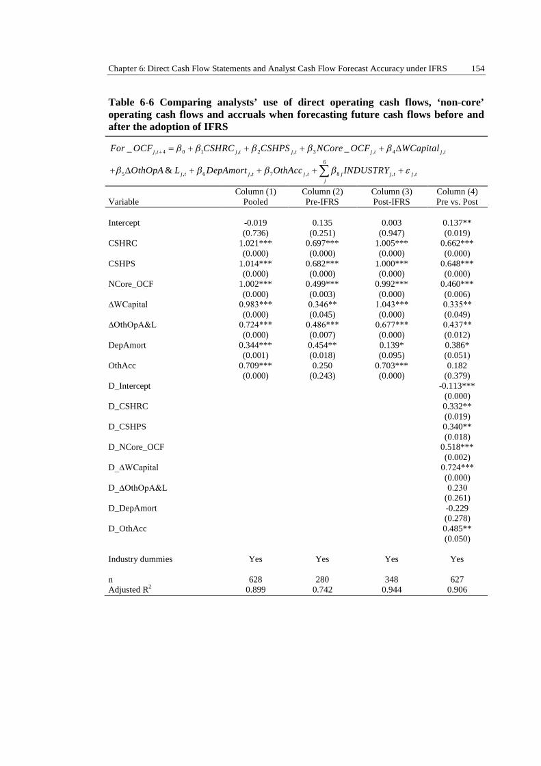
Chapter 6: Direct Cash Flow Statements and Analyst Cash Flow Forecast Accuracy under IFRS 154
Table 6-6 Comparing analysts’ use of direct operating cash flows, ‘non-core’operating cash flows and accruals when forecasting future cash flows before andafter the adoption of IFRS
, 4 0 1 , 2 , 3 , 4 ,
6
5 , 6 , 7 , 8 , ,
_ _
&
j t j t j t j t j t
j t j t j t j j t j tj
For OCF CSHRC CSHPS NCore OCF WCapital
OthOpA L DepAmort OthAcc INDUSTRY
Column (1) Column (2) Column (3) Column (4)Variable Pooled Pre-IFRS Post-IFRS Pre vs. Post
Intercept -0.019 0.135 0.003 0.137**(0.736) (0.251) (0.947) (0.019)
CSHRC 1.021*** 0.697*** 1.005*** 0.662***(0.000) (0.000) (0.000) (0.000)
CSHPS 1.014*** 0.682*** 1.000*** 0.648***(0.000) (0.000) (0.000) (0.000)
NCore_OCF 1.002*** 0.499*** 0.992*** 0.460***(0.000) (0.003) (0.000) (0.006)
∆WCapital 0.983*** 0.346** 1.043*** 0.335** (0.000) (0.045) (0.000) (0.049)
∆OthOpA&L 0.724*** 0.486*** 0.677*** 0.437** (0.000) (0.007) (0.000) (0.012)
DepAmort 0.344*** 0.454** 0.139* 0.386*(0.001) (0.018) (0.095) (0.051)
OthAcc 0.709*** 0.250 0.703*** 0.182(0.000) (0.243) (0.000) (0.379)
D_Intercept -0.113***(0.000)
D_CSHRC 0.332**(0.019)
D_CSHPS 0.340**(0.018)
D_NCore_OCF 0.518***(0.002)
D_∆WCapital 0.724*** (0.000)
D_∆OthOpA&L 0.230 (0.261)
D_DepAmort -0.229(0.278)
D_OthAcc 0.485**(0.050)
Industry dummies Yes Yes Yes Yes
n 628 280 348 627Adjusted R2 0.899 0.742 0.944 0.906
Chapter 6: Direct Cash Flow Statements and Analyst Cash Flow Forecast Accuracy under IFRS 155
Table 6-6 (continued)“Pooled” regressions include all firms spanning both the pre and post-IFRS period between January 2000and December 2010. “Pre-IFRS” includes all firms with financial years ending up to and includingDecember 31, 2004, whereas “Post-IFRS” incorporates all firms with financial years ending on or afterJanuary 1, 2005. “Pre vs. Post” are pooled regressions, which include interactive dummy variables toinvestigate the change in significance of the explanatory variables after the adoption of IFRS. Whenestimating the coefficients’ standard errors, a White (1980) procedure is used to correct forheteroskedasticity. Variable definitions are as reported in Table 6-2. Dummy variables are prefixed by“D”, taking on the value of their respective explanatory variable post-IFRS, and zero otherwise. Two-tailed p-values are presented in parentheses. *** p<0.01, ** p<0.05, * p<0.1.
Presenting results from Equation (6.4), Table 6-7 provides consistent support for the
first hypotheses. The mean coefficients for CSHRC and CSHPS remain significantly
positive pre and post-IFRS and continue to show a significant increase in significance
post-IFRS. Further, Table 6-7 provides evidence that disaggregating NCore_OCF into
the components of interest paid (INTP), net taxes received or paid (TXP) and other
operating cash flows (CSHOTH) provide analysts with useful information post-IFRS.
However, pre-IFRS TXP, ΔWCapital, DepAmort and OthAcc are insignificant. Other
than the change in the mean coefficient for INTP, column 4 provides strong support for
H1b by showing a significant improvement in the usefulness of direct cash flow
components and aggregate accruals since the adoption of IFRS. In summary, these
findings show financial analysts’ do use ‘core’ direct cash flow components when
forecasting cash flows, and that the usefulness of this information significantly
increases post-IFRS.
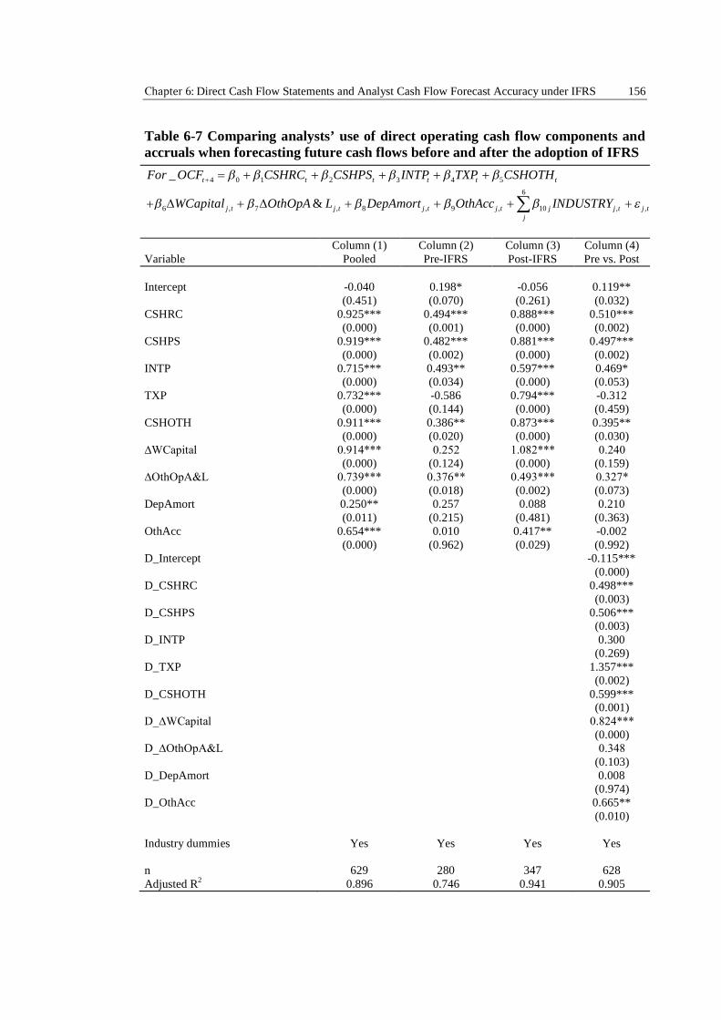
Chapter 6: Direct Cash Flow Statements and Analyst Cash Flow Forecast Accuracy under IFRS 156
Table 6-7 Comparing analysts’ use of direct operating cash flow components andaccruals when forecasting future cash flows before and after the adoption of IFRS
4 0 1 2 3 4 5
6
6 , 7 , 8 , 9 , 10 , ,
_
&
t t t t t t
j t j t j t j t j j t j tj
For OCF CSHRC CSHPS INTP TXP CSHOTH
WCapital OthOpA L DepAmort OthAcc INDUSTRY
Column (1) Column (2) Column (3) Column (4)Variable Pooled Pre-IFRS Post-IFRS Pre vs. Post
Intercept -0.040 0.198* -0.056 0.119**(0.451) (0.070) (0.261) (0.032)
CSHRC 0.925*** 0.494*** 0.888*** 0.510***(0.000) (0.001) (0.000) (0.002)
CSHPS 0.919*** 0.482*** 0.881*** 0.497***(0.000) (0.002) (0.000) (0.002)
INTP 0.715*** 0.493** 0.597*** 0.469*(0.000) (0.034) (0.000) (0.053)
TXP 0.732*** -0.586 0.794*** -0.312(0.000) (0.144) (0.000) (0.459)
CSHOTH 0.911*** 0.386** 0.873*** 0.395**(0.000) (0.020) (0.000) (0.030)
∆WCapital 0.914*** 0.252 1.082*** 0.240 (0.000) (0.124) (0.000) (0.159)
∆OthOpA&L 0.739*** 0.376** 0.493*** 0.327* (0.000) (0.018) (0.002) (0.073)
DepAmort 0.250** 0.257 0.088 0.210(0.011) (0.215) (0.481) (0.363)
OthAcc 0.654*** 0.010 0.417** -0.002(0.000) (0.962) (0.029) (0.992)
D_Intercept -0.115***(0.000)
D_CSHRC 0.498***(0.003)
D_CSHPS 0.506***(0.003)
D_INTP 0.300(0.269)
D_TXP 1.357***(0.002)
D_CSHOTH 0.599***(0.001)
D_∆WCapital 0.824*** (0.000)
D_∆OthOpA&L 0.348 (0.103)
D_DepAmort 0.008(0.974)
D_OthAcc 0.665**(0.010)
Industry dummies Yes Yes Yes Yes
n 629 280 347 628Adjusted R2 0.896 0.746 0.941 0.905
Chapter 6: Direct Cash Flow Statements and Analyst Cash Flow Forecast Accuracy under IFRS 157
Table 6-7 (continued)“Pooled” regressions include all firms spanning both the pre and post-IFRS period between January 2000and December 2010. “Pre-IFRS” includes all firms with financial years ending up to and includingDecember 31, 2004, whereas “Post-IFRS” incorporates all firms with financial years ending on or afterJanuary 1, 2005. “Pre vs. Post” are pooled regressions, which include interactive dummy variables toinvestigate the change in significance of the explanatory variables after the adoption of IFRS. Whenestimating the coefficients’ standard errors, a White (1980) procedure is used to correct forheteroskedasticity. Variable definitions are as reported in Table 6-2. Dummy variables are prefixed by“D”, taking on the value of their respective explanatory variable post-IFRS, and zero otherwise. Two-tailed p-values are presented in parentheses. *** p<0.01, ** p<0.05, * p<0.1.
6.4.4 IFRS Adoption and Accuracy of Analysts’ Cash Flow Forecasts
Having established financial analysts use direct cash flow components when forecasting
cash flows, and significantly more so under IFRS, it now remains to examine whether
their cash flow forecasts are significantly more accurate post-IFRS, and whether
financial analysts, by using direct cash flow components, can significantly improve the
accuracy of their cash flow predictions. Coefficient estimates from the ordinary least-
squares regression of Equation (6.6), investigating the second hypothesis, are presented
in Table 6-8 in columns 1 through 3. Following Hodder et al. (2008), standard errors are
adjusted to control for firm level clustering over time.
Column 1 displays the primary results and estimated coefficients for the entire
sample of firms pooled from January 2000 to December 2010. The intercept is positive
and significant (coefficient of 0.273; two-tailed p-value < 0.01). Further, the mean
coefficient for the main variable of interest (IFRS), which measures the change in
analyst cash flow forecast error since the adoption of IFRS is negative and highly
significant (coefficient of -0.014; two-tailed p-value < 0.01).

Chapter 6: Direct Cash Flow Statements and Analyst Cash Flow Forecast Accuracy under IFRS 158
Table 6-8 Effect of mandatory IFRS adoption on analysts’ cash flow forecasterrors
, 0 1 2 , 6 1 3 , 6 1 4 , 1
5 , 1 6 , 1 7 , 1 8 , 1
6
9 , 1 10 , 1 11 , 1 ,_
j T j T toT j T toT j T
j T j T j T j T
j T j T j T j Tj
AFE IFRS OCF WCA MIXED
NEGOCF SIZE GROWTH PROFITABILITY
NANAL OP CYCLE INDUSTRY
Variable
ExpectedSign
Column (1)Pooled
Column (2)Financial
Crises
Column (3)All controls
Intercept n/a 0.273*** 0.269*** 0.264***(0.000) (0.000) (0.000)
IFRS -ve -0.014*** -0.011** -0.014**(0.008) (0.038) (0.019)
OCFT-6 to T-1 +ve 0.042** 0.043*** 0.042***(0.012) (0.007) (0.007)
DWCAT-6 to T-1 +ve 0.010 0.007 0.007(0.626) (0.717) (0.701)
MIXEDT-1 +ve -0.002 -0.002 -0.002(0.473) (0.636) (0.600)
NEGOCFT-1 +ve 0.027 0.022 0.023(0.297) (0.394) (0.390)
SIZET-1 ? -0.009*** -0.009*** -0.009***(0.000) (0.000) (0.000)
GROWTHT-1 ? 0.020*** 0.020*** 0.020***(0.000) (0.000) (0.000)
PROFITABILITYT-1 ? -0.057 -0.067 -0.066(0.178) (0.148) (0.150)
NANALT-1 ? -0.017*** -0.023*** -0.025***(0.007) (0.001) (0.001)
OP_CYCLET-1 +ve -0.017 -0.017 -0.017(0.349) (0.350) (0.339)
D_CRISIS_02 +ve 0.021** 0.021**(0.012) (0.011)
D_CRISIS_08 +ve 0.015*** 0.017***(0.000) (0.000)
D_2005 +ve 0.007*(0.091)
Industry dummies Yes Yes Yes
n 525 525 525Adjusted R2 0.200 0.225 0.225All regressions are pooled and include all firms spanning both the pre and post-IFRS period betweenJanuary 2000 and December 2010. Clustered standard errors are used to correct for firm level serialdependence over the sample period. Column (1) provides results from the base model using Equation (6)where IFRS is a dummy variable equal to 1 if the financial year-end is after January 1, 2005, and 0otherwise. Column (2) includes two additional dummy variables, D_CRISIS_02 and D_CRISIS_08,controlling for analysts’ forecasts made during times of the respective stock market crises for thefinancial years prior to 2002 and after 2007. Column (3) includes a final additional dummy variable,D_2005, controlling for analyst forecasts made for the financial year 2005, the year of IFRS adoption. Allremaining variable definitions are as reported in Table 6-2. Two-tailed p-values are presented in
Chapter 6: Direct Cash Flow Statements and Analyst Cash Flow Forecast Accuracy under IFRS 159
parentheses. *** p<0.01, ** p<0.05, * p<0.1.
These findings are consistent with the prediction and univariate results that analysts’
cash flow forecast accuracy improves after the adoption of IFRS. Additionally,
, 6 1j T to TOCF and , 1j TGROWTH are significant and positively related to analyst
forecast errors (coefficients of 0.042 and 0.020; two-tailed p-values < 0.05 and <0.01
respectively), while , 1j TSIZE and , 1j TNANAL are significant and negatively related to
analyst forecast errors (coefficients of -0.009 and -0.017; two-tailed p-value < 0.01).
Column 2 re-examines the second hypothesis by controlling for all forecasts made
for financial years prior to 2002 and after 2007 to avoid any confounding effects on the
results from the 2001 and 2008 market crashes, since analysts forecast errors are
expected to increase significantly during times of uncertainty. Consistent with the
predictions and previous findings, IFRS remains negative and significant in column 2
(coefficients of -0.011; two-tailed p-value < 0.05), while the magnitude and significance
of the coefficients for , 6 1j T to TOCF , , 1j TGROWTH , , 1j TSIZE and , 1j TNANAL remain
largely similar to those reported in column 1. As expected the coefficients on the two
control variables for the market crashes, D_CRISIS_02 and D_CRISIS_08, are positive
and significant indicating an increase in analysts cash flow forecast errors during times
of significant market volatility.
Finally, following Horton et al. (2012), column 3 includes control for all analyst
forecasts made for the year of IFRS adoption and presents consistent findings with
columns 1 and 2 where IFRS remains negative and significant (coefficients of -0.014;
two-tailed p-value < 0.05). Results for the remaining control variables are consistent
with those in columns 1 and 2 and the control for the year of IFRS adoption is positive
and marginally significant (coefficient of 0.007; two-tailed p-value < 0.10). Analyst
Chapter 6: Direct Cash Flow Statements and Analyst Cash Flow Forecast Accuracy under IFRS 160
cash flow forecast errors marginally increased during the year of IFRS adoption. In
summary, these findings provide strong support for the second hypothesis that analysts’
cash flow forecast accuracy improves subsequent to the adoption of IFRS. These
findings are in line with prior studies that show analysts’ earnings forecast accuracy
also improves post-IFRS, and supports the view that the adoption of IFRS has
significantly improved the quality of information available to financial analysts.
6.4.5 Ranking the Empirical Models
The results so far reveal analysts use net operating cash flows and direct cash flow
components to predict cash flows for the entire sample period, finding direct cash flow
components more useful under IFRS, and forecasting cash flows more accurately under
IFRS. However, it remains to be seen whether the improvement in forecast accuracy
under IFRS is due to the increased differential usefulness of direct cash flow
components under IFRS. Following Krishnan and Largay III (2000), therefore,
Friedman’s ANOVA rank tests are used to examine H2b, of whether there is a
significant difference between absolute forecast errors calculated for each of Equations
(6.1) to (6.4). Table 6-9 reports the Friedman’s ANOVA statistics, along with the
results of t-tests comparing the average rank and forecast error for each model between
the pre and post-IFRS periods.
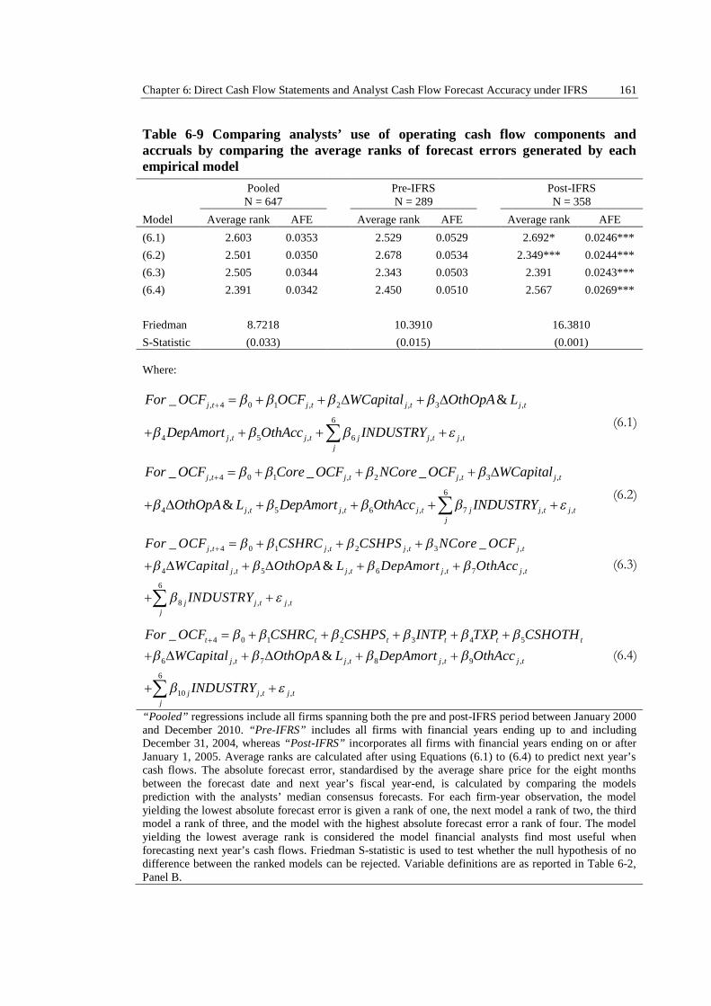
Chapter 6: Direct Cash Flow Statements and Analyst Cash Flow Forecast Accuracy under IFRS 161
Table 6-9 Comparing analysts’ use of operating cash flow components andaccruals by comparing the average ranks of forecast errors generated by eachempirical model
PooledN = 647
Pre-IFRSN = 289
Post-IFRSN = 358
Model Average rank AFE Average rank AFE Average rank AFE
(6.1) 2.603 0.0353 2.529 0.0529 2.692* 0.0246***
(6.2) 2.501 0.0350 2.678 0.0534 2.349*** 0.0244***
(6.3) 2.505 0.0344 2.343 0.0503 2.391 0.0243***
(6.4) 2.391 0.0342 2.450 0.0510 2.567 0.0269***
Friedman 8.7218 10.3910 16.3810
S-Statistic (0.033) (0.015) (0.001)
Where:
, 4 0 1 , 2 , 3 ,
6
4 , 5 , 6 , ,
_ &j t j t j t j t
j t j t j j t j tj
For OCF OCF WCapital OthOpA L
DepAmort OthAcc INDUSTRY
(6.1)
, 4 0 1 , 2 , 3 ,
6
4 , 5 , 6 , 7 , ,
_ _ _
&
j t j t j t j t
j t j t j t j j t j tj
For OCF Core OCF NCore OCF WCapital
OthOpA L DepAmort OthAcc INDUSTRY
(6.2)
, 4 0 1 , 2 , 3 ,
4 , 5 , 6 , 7 ,
6
8 , ,
_ _
&
j t j t j t j t
j t j t j t j t
j j t j tj
For OCF CSHRC CSHPS NCore OCF
WCapital OthOpA L DepAmort OthAcc
INDUSTRY
(6.3)
4 0 1 2 3 4 5
6 , 7 , 8 , 9 ,
6
10 , ,
_
&
t t t t t t
j t j t j t j t
j j t j tj
For OCF CSHRC CSHPS INTP TXP CSHOTH
WCapital OthOpA L DepAmort OthAcc
INDUSTRY
(6.4)
“Pooled” regressions include all firms spanning both the pre and post-IFRS period between January 2000and December 2010. “Pre-IFRS” includes all firms with financial years ending up to and includingDecember 31, 2004, whereas “Post-IFRS” incorporates all firms with financial years ending on or afterJanuary 1, 2005. Average ranks are calculated after using Equations (6.1) to (6.4) to predict next year’scash flows. The absolute forecast error, standardised by the average share price for the eight monthsbetween the forecast date and next year’s fiscal year-end, is calculated by comparing the modelsprediction with the analysts’ median consensus forecasts. For each firm-year observation, the modelyielding the lowest absolute forecast error is given a rank of one, the next model a rank of two, the thirdmodel a rank of three, and the model with the highest absolute forecast error a rank of four. The modelyielding the lowest average rank is considered the model financial analysts find most useful whenforecasting next year’s cash flows. Friedman S-statistic is used to test whether the null hypothesis of nodifference between the ranked models can be rejected. Variable definitions are as reported in Table 6-2,Panel B.
Chapter 6: Direct Cash Flow Statements and Analyst Cash Flow Forecast Accuracy under IFRS 162
Using Equations (6.1) to (6.4), next year’s cash flows are predicted and compared
with the analysts’ median consensus forecasts. Then, the absolute, price standardised,
forecast error is calculated by using Equation (6.5). For each firm-year observation, the
model with the lowest absolute forecast error is ranked as 1, the next model ranked 2,
the third model ranked 3, and the model with the highest absolute forecast error ranked
4. The model yielding the lowest average rank will be the model containing the cash
flow information financial analysts find most useful when forecasting next year’s cash
flows.
Consistent with Krishnan and Largay III (2000), Table 6-9 reports the lowest average
rank for Equations (6.3) and (6.4), when OCF is disaggregated into CSHRC and CSHPS,
on a pooled basis and under local GAAP. However, under IFRS, Equations (6.2) and
(6.3) are found to yield the lowest average rank and absolute forecast errors with the
average rank of Equation (6.2), using ‘core’ direct cash flow information, falling
significantly post-IFRS. Conversely, the average rank for Equation (6.1), using
aggregate operating cash flows, rose marginally in the post-IFRS period. Friedman S-
statistics are significant at the 5% level for both the pooled and pre-IFRS periods and at
the 1% level post-IFRS.
Taken together, these results imply that analysts consider more information than just
aggregate operating cash flows and accruals components when forecasting cash flows.
Analysts’ clearly find information about the cash receipts from customers and cash
payments to suppliers and employees, which can only be found in direct cash flow
statements, more useful than aggregate operating cash flows when predicting next
year’s cash flows. Further, consistent with the earlier findings, analysts cash flow
forecast accuracy significantly improves under IFRS. These findings support the
Chapter 6: Direct Cash Flow Statements and Analyst Cash Flow Forecast Accuracy under IFRS 163
hypothesis that the significant improvement in analysts’ cash flow forecasts post-IFRS
is significantly associated to the significant increase in the usefulness of direct cash
flow components by financial analysts’ post-IFRS.
6.5 Discussion and Conclusion
Current FASB and IASB proposals to mandate direct cash flow statements are
motivated by the assertion that the direct method provides information, unavailable
from the indirect method, which is useful in forecasting cash flows. Prior studies
examining this assertion have used random walk models, and find a significant increase
in forecast accuracy after including historical direct cash flow components within their
models (e.g., Krishnan and Largay III, 2000; Arthur and Chuang, 2008; Cheng and
Hollie, 2008; Orpurt and Zang, 2009; Arthur et al., 2010; Farshadfar and Monem, 2012,
2013). Importantly, however, while these findings complement financial analysts’
opinions that direct cash flows provide useful information to forecast future cash flows,
to date, no research has empirically examined, when available, if financial analysts
actually use this information when forecasting future cash flows. Further, since the
adoption of IFRS, after which the quality and comparability of information available to
financial analysts significantly improved (Bissessur and Hodgson, 2011; Cotter et al.,
2012), no research has examined analysts’ use of direct cash flows when predicting
future cash flows or the change in analysts’ cash flow forecast accuracy.
By mandating the use of direct cash flow statements until 2007, and prohibiting the
early voluntary adoption of IFRS, Australia provides an ideal setting to test financial
analysts’ use of direct cash flow components when forecasting future cash flows under
both local GAAP and IFRS, and to compare the change between the two periods. The
Chapter 6: Direct Cash Flow Statements and Analyst Cash Flow Forecast Accuracy under IFRS 164
results provide strong evidence that financial analysts use information from direct cash
flow statements when estimating future cash flows under both local GAAP and IFRS,
but more so since the adoption of IFRS. Moreover, they show a strong post-IFRS
improvement in the accuracy of analysts’ cash flow predictions, which is likely a result
of financial analysts finding information about direct cash flow components
significantly more useful under IFRS. Taken together, these findings affirm financial
analyst’s opinions that information from direct cash flow statements is useful when
estimating future cash flows, and are consistent with IFRS improving analysts’
information environment. By requiring the use of direct cash flow statements, the FASB
and IASB would be providing financial analysts with useful information, which in turn
would provide investors with more accurate cash flow predictions on which to base
their economic decisions.
The final empirical chapter, therefore, examines whether financial analysts use their
cash flow forecasts and information from direct cash flow statements as inputs in the
process of arriving at their final output, the stock recommendation. Further, chapter 7
examines whether buy-and-hold investors are better able to identify mispriced securities
by following the analysts’ recommendations or by using analysts’ cash flow forecasts in
discounted cash flow valuation models.
Chapter 7: Direct Cash Flows, Analysts’ Cash Flow Forecasts and Stock Recommendations 165
7Are Analysts’ Cash Flow Forecasts andDirect Cash Flow Statements EssentialInputs to Generate StockRecommendations?
7.1 Introduction
Prior studies demonstrate that analysts’ stock recommendations relate positively to
valuation heuristics based on their earnings forecasts, but negatively to future excess
stock returns and residual income valuations scaled by current price (Bradshaw, 2004;
Barniv et al., 2009, 2010). While these studies validate the use of analysts’ earnings
forecasts as valuation inputs to identify mispriced securities, the extant literature has, to
date, not analysed whether analysts’ cash flow forecasts are used in a similar manner.
Increasingly, analysts are forecasting both earnings and cash flows, partly in response to
increased market demand for price relevant information (DeFond and Hung, 2003).
Historical operating cash flows have been found to increase in value relevance for firms
where analysts forecast earnings and cash flows compared to those where only earnings
are forecast (Call, 2008). Moreover, significant positive market reactions are observed
within four days of analysts revising their cash flow forecasts, further demonstrating the
value relevant information provided over and above analysts’ earnings forecasts (Call et
al., 2012). This chapter, therefore, hypothesises that analysts’ cash flow forecasts
provide analysts and investors with valuable information to identify mispriced securities.
Chapter 7: Direct Cash Flows, Analysts’ Cash Flow Forecasts and Stock Recommendations 166
Historical operating cash flows are one of many sources that provide financial
analysts with valuable information when forecasting cash flows. Moreover, assessing an
entities ability to generate future cash flows is one of the main benefits of preparing a
cash flow statement according to International Accounting Standard 7, which states:
“Historical cash flow information is often used as an indicator of the amount,
timing and certainty of future cash flows.”
(IASB, 2010, paragraph 5)
Further, a recent large-scale survey by the Chartered Financial Analysts Institute
revealed that most analysts believe direct, rather than indirect, cash flow statements
provide useful information for forecasting cash flows. Accordingly, this chapter
examines whether historical direct cash flow statements provide financial analysts with
valuable information when issuing their stock recommendations.
By using a sample of non-financial Australian companies listed on the ASX300 from
2000-2010, and following Bradshaw (2004), analysts’ earnings forecasts are used to
construct residual income valuation models and heuristics. Adopting a similar approach
to the development of these models, analysts’ cash flow forecasts are then used to
construct discount cash flow valuation models and heuristics. Analysts’ consensus stock
recommendations, and future excess stock returns, are then compared to the price
standardised values produced by the residual income models, and discounted cash flow
models. Further, analysts’ stock recommendations, and future excess stock returns, are
compared to a number of heuristics based on analysts’ earnings, cash flow, and long-
term growth forecasts, and heuristics based on historical earnings and cash flows.
Chapter 7: Direct Cash Flows, Analysts’ Cash Flow Forecasts and Stock Recommendations 167
Finally, to identify which model best identifies mispriced securities, Vuong (1989) tests
are used to compare the explanatory power between the various earnings and cash flow
based models.
The findings of this chapter demonstrate that financial analysts do use their cash flow
forecasts and historical direct cash flow information when setting stock
recommendations. However, analyst stock recommendations relate negatively to future
excess stock returns and discount cash flow models scaled by current price. Overall, the
results are consistent with the earnings based studies, and demonstrate that buy-and-
hold investors are better off using analysts’ forecasts in multi-period valuation models
to identify mispriced securities compared to following analysts’ recommendations.
Moreover, in comparison to the profitability of using multi-period earnings valuation
techniques, buy-and-hold investors are significantly better off by using analyst cash
flow forecasts in discounted cash flow models to identify mispriced securities.
7.2 Background and Hypothesis Development
7.2.1 Analysts’ Choice of Valuation Model
There is a substantial literature on the valuation models employed by analysts to
identify mispriced stocks when issuing their recommendations and price forecasts.
Surveys and interviews, particularly popular methods of investigating analysts’
valuation model preferences, generally find most prefer price-earnings valuation
heuristics to multi-period valuation techniques. Nearly half the respondents in a 1998
U.S. survey of the Association of Investment Management and Research (AIMR)
members never used present value (PV) techniques when valuing stocks in practice
Chapter 7: Direct Cash Flows, Analysts’ Cash Flow Forecasts and Stock Recommendations 168
(Block, 1999). However, they still considered earnings and cash flow information the
most important inputs in the stock valuation process.
Moreover, in a concurrent U.K. study, analysts and fund managers also indicated
their preference for simple valuation techniques (Barker, 1999). Price-earnings,
dividend-yield, and price-cash flow models were all ranked more highly than
discounted cash flow and dividend discount valuation models. Analysts preferred
valuation heuristics because of the difficultly in reliably estimating multi-period
valuation models, which can be sensitive to various underlying assumptions.
Consequently, when estimating the value of a stock beyond a two-year horizon, analysts
preferred using their subjective judgement. These findings confirm the results of earlier
surveys and interviews, which all reveal a distinct analyst preference for price-earnings
valuation techniques over discounting models (Arnold and Moizer, 1984; Moizer and
Arnold, 1984; Pike et al., 1993).
A popular alternative method of investigating analysts’ valuation model choice is by
analysing their reports. Results from U.S. content analysis studies further corroborate
the interviews and surveys, and reveal analysts predominantly use price-earnings
valuation heuristics over multi-period techniques (Previts et al., 1994; Bradshaw, 2002;
Asquith et al., 2005). Moreover, while U.K. studies reveal an increasing number of
analysts using discounted cash flow methods as a dominant valuation technique, price-
earnings methods continued to be used as a major valuation tool (Demirakos et al., 2004;
Imam et al., 2008). In addition to price-earnings ratios, Bradshaw (2002) observe
analysts regularly use their long-term growth projections to justify issuing favourable
stock recommendations and price forecasts. Moreover, by combining the price-earnings
ratio, calculated using analysts’ forecast earnings, with their long-term growth
Chapter 7: Direct Cash Flows, Analysts’ Cash Flow Forecasts and Stock Recommendations 169
projections, Bradshaw (2002) constructs a price-earnings-growth ratio (PEG) which he
then compares to the analyst recommendations. He observes that, when analysts issue
recommendations and price targets, the PEG ratio is positively and significantly
associated with their recommendation. However, when analysts only issued a
recommendation, and did not issue a price target, the PEG model failed to provide a
meaningful justification for the recommendation. One possible explanation for these
findings could be that analysts, issuing a stock recommendation without a price forecast,
lack confidence in the inputs of, and therefore the results from, their valuation models
(Bradshaw, 2002). Price targets are, after all, far less opaque than stock
recommendations and provide investors with a better benchmark against which to
measure analyst performance. Consequently, it is increasingly important to examine not
only which valuation models are predominantly used by analysts, but also which
valuation inputs are used in these models.
7.2.2 Analysts’ Earnings Forecasts as Valuation Inputs
Surveys, interviews, and content analysis studies consistently show analysis prefer
simple valuation heuristics over multi-period valuation models when determining
whether a stock is mispriced for the purposes of issuing their stock recommendation.
However, while viewed as their final output, issuing a stock recommendation is
essentially the result of a process that generally includes analysts issuing forecasts for
both earnings and cash flows (Schipper, 1991; Brown, 1993). To better understand this
process, Schipper (1991) and Brown (1993) both call for empirical research examining
the link between analysts’ recommendations and their forecasts.
In response to Schipper (1991) and Brown (1993), Bradshaw (2004) provides some
of the first empirical evidence that financial analysts do make use of their earnings
Chapter 7: Direct Cash Flows, Analysts’ Cash Flow Forecasts and Stock Recommendations 170
forecasts when issuing stock recommendations. By using a sample of U.S. firms
between 1994 and 1998, and following Bradshaw (2002) to construct a PEG heuristic
using analysts’ earnings and growth forecasts, Bradshaw (2004) finds a significant
positive relationship between his PEG heuristic and analysts stock recommendations.
Moreover, analysts’ long-term earnings growth forecasts are also significantly and
positively associated with their stock recommendations. In contrast, however, Bradshaw
(2004) observes a counterintuitive negative relationship between the price standardised
residual income valuation, also calculated using analysts’ earnings forecasts, and their
stock recommendation. Analysts appear to issue negative/(positive) recommendations
when the residual income valuation is greater/(lower) than the current share price.
While analysts use their earnings forecasts in simple valuation heuristics, they do not
appear to use them in more complex multi-period valuation models when issuing their
recommendations. However, Bradshaw (2004) does find a significant positive
relationship between one-year-ahead size-adjusted returns and the residual income
valuation. These findings imply that it would be more profitable for buy-and-hold
investors to use analysts’ earnings forecasts in multi-period residual income models,
rather than following the analysts’ recommendations.
Barniv et al. (2009) and Barniv et al. (2010) both extend Bradshaw’s (2004) study,
and provide further evidence of a significant positive relationship between valuation
heuristics based on analysts’ earnings forecasts and their stock recommendations. By
expanding the sample period from 1993 to 2005, Barniv et al. (2009) examines the
impact of regulatory changes in the U.S. financial analyst industry on the process by
which analysts’ arrive at their stock recommendations. Prior to the introduction of
Chapter 7: Direct Cash Flows, Analysts’ Cash Flow Forecasts and Stock Recommendations 171
Regulation Fair Disclosure53 (Reg FD) in 2000, they observe very similar findings to
Bradshaw (2004). However, subsequent to Reg FD they find a significant decline in the
negative relationship between recommendations and residual income valuations. These
results suggest that the regulatory reforms in the U.S. have increased analyst discipline,
and subsequently increased the quality of their recommendations. However, irrespective
of the time period used, their results still reveal analysts continue to use PEG and long-
term earnings growth heuristics when issuing their recommendations. Moreover,
analysts’ stock recommendations continue to relate negatively to future size-adjusted
returns. Consequently, investors are continually better off using analysts’ earnings
forecasts in a multi-period residual income valuation model to identify mispriced stocks
compared to relying on analysts’ recommendations.
More recently, in an international study between 1993 and 2007, Barniv et al. (2010)
investigate whether a country’s level of investor participation influences analysts’ use
of valuation heuristics compared to multi-period valuation methods when
recommending stocks. Their results from high investor participation countries,
including Australia, support Bradshaw’s (2004) findings. Their results from low
investor participation countries, however, reveal a significantly less negative, and in one
case a positive relationship, between analysts’ recommendations and residual income
valuations using analysts’ earnings forecasts. Analysts’ recommendations generally
appear to be less biased in low investor participation countries than high investor
participation countries. In high participation countries, analysts appear to follow the
historical trend observed in U.S. studies of issuing biased optimistic stock
53 Regulation Fair Disclosure was introduced in the U.S. by the Securities Exchange Commission (SEC)on 15 August 2000, to regulate the disclosure of non-public information to select individuals, such asanalysts. Disclosures of non-public information to analysts must now to be disclosed to the public at thesame time.
Chapter 7: Direct Cash Flows, Analysts’ Cash Flow Forecasts and Stock Recommendations 172
recommendations. Barniv et al. (2010) conclude that this bias is likely due to the greater
numbers of smaller, less sophisticated, investors in high investor participation countries
which naïvely follow analysts’ recommendations.
7.2.3 Analysts’ Cash Flow Forecasts as Valuation Inputs
Bradshaw (2004), Barniv et al. (2009), and Barniv et al. (2010) all demonstrate analysts
use their earnings forecasts in valuation heuristics when recommending stocks, however,
to date, no research has examined how analysts make use of their cash flow forecasts
when recommending stocks. Schipper (1991) and Brown (1993) both assert that analyst
forecasts are fundamental inputs in the process of analysts determining their
recommendations. Accordingly, not only analysts’ earnings forecasts, but also their
cash flow forecasts should provide useful information in evaluating whether stocks are
mispriced in the process of arriving at their final recommendation.
While analysts have been issuing earnings forecasts for decades, the frequency of
analysts issuing cash flow forecasts, alongside their earnings forecasts, is increasing.
Evidence from a recent international study by DeFond and Hung (2007) shows a rise in
the numbers of analysts forecasting both cash flows and earnings from 30% in 1994 up
to 58% by 2002. This growing number of analysts forecasting cash flows is partly due
to increased market demand for price relevant information, especially for firms with
volatile earnings, high levels of accruals and poor financial health (DeFond and Hung,
2003). Moreover, analysts who issue both earnings and cash flow forecasts have been
found to issue significantly more accurate earnings forecasts (Call et al., 2009), while at
the same time providing an external deterrent to earnings management (Call, 2008;
McInnis and Collins, 2011).
Chapter 7: Direct Cash Flows, Analysts’ Cash Flow Forecasts and Stock Recommendations 173
Although prior research show analysts predominantly use price-earnings valuation
heuristics, content analysis studies show some analysts also use cash flow valuation
heuristics or discounted cash flow techniques as part of the stock evaluation process.
Asquith et al. (2005) finds evidence that discounted cash flow techniques were utilised
in 13% of their sample, while Demirakos et al. (2004) observe that, for their sample, 38%
of analysts use DCF techniques, with 20% using DCF as the dominant valuation method.
When choosing between multi-period models, analysts appeared to prefer DCF as
Demirakos et al. (2004) find less than 2% of the reports reveal any reference to analysts’
use of residual income valuation techniques. Moreover, single period “price-cash flow”
ratios were used, on several occasions, to check the dominant valuation model’s results.
Further, extending Demirakos et al. (2004), Imam et al. (2008) observed 62% of the 98
U.K. analyst reports referred to cash flow based models as the dominant valuation
technique when recommending stocks.
Evidence that analysts find cash flow information useful to identify mispriced
securities comes as no surprise given the asserted benefits provided by a Statement of
Cash Flows as documented by the Financial Accounting Standards Board (FASB) and
International Accounting Standards Board (IASB). For example, IAS 7 states that:
“Cash flow information is useful in assessing the ability of the entity to generate
cash and cash equivalents and enables users to develop models to assess and
compare the present value of the future cash flows of different entities.”
(IASB, 2010, paragraph 4)

Chapter 7: Direct Cash Flows, Analysts’ Cash Flow Forecasts and Stock Recommendations 174
Discounted projections of future cash flows should provide, therefore, a reasonable
benchmark against which to compare the current market price, and so identify whether
or not the stock is mispriced. Further, confirming the usefulness of cash flow
information to identify mispriced stocks, Sloan (1996) observes how portfolios of firms
with high levels of reported cash flows earned positive abnormal annual stock returns
compared to portfolios with high levels of accruals. Whilst Sloan (1996) highlights
possible shortcomings to developing a trading strategy of taking a long/short position
for stocks with high/low levels of cash flows relative to accruals, cash flow information
is still clearly useful in the process of identifying mispriced securities.
Prior empirical research has demonstrated that analysts do make use of their earnings
forecasts by using heuristic valuations, such as the PEG model, to identify mispriced
stocks (Bradshaw, 2004; Barniv et al., 2009, 2010). However, no empirical research has
considered whether analysts also use their cash flow forecasts in heuristic valuations to
identify mispriced securities in the process of determining their final recommendation.
Cash flow information has been shown to be useful in identifying mispriced stocks
(Sloan, 1996), and growing numbers of analysts have been issuing cash flow forecasts
alongside their earnings forecasts (DeFond and Hung, 2007). Accordingly, if analysts
use valuation heuristics based on their cash flow forecasts to identify mispriced stocks,
then there should be a positive relationship between these heuristics and their stock
recommendations. Hence, the first hypothesis to be presented is:
H1a: Analysts issue more/less favourable recommendations for high/low heuristic
valuations based on analysts’ forecast cash flows or earnings
Chapter 7: Direct Cash Flows, Analysts’ Cash Flow Forecasts and Stock Recommendations 175
7.2.3.1 Usefulness of Direct Cash Flow Information
Financial analysts were strongly in favour of the recent joint proposal from The
International Accounting Standards Board (IASB) and Financial Accounting Standards
Board (FASB) to mandate direct cash flow statements. 54 Analyst support for the
proposal was based largely on their commonly held opinion that direct cash flow
statements provide better information for forecasting future cash flows and measuring
earnings quality than indirect cash flow statements.55 Their viewpoint is strongly backed
by a number of empirical studies which show that direct cash flow statements provide
incremental information when forecasting future cash flows (e.g., Krishnan and Largay
III, 2000; Orpurt and Zang, 2009; Arthur et al., 2010; Farshadfar and Monem, 2012,
2013).
Given analysts strong support of the current proposal to mandate the use of direct
cash flow statements, Hales and Orpurt (2012) questioned whether, when available,
analysts would actually make use of information from direct cash flow statements when
forecasting cash flows, or issuing stock recommendations. If analysts use valuation
heuristics based on direct cash flow information to identify mispriced stocks, then there
should be a positive relationship between these heuristics and their stock
recommendations. Accordingly, H1b is:
H1b: Analysts issue more/less favourable recommendations for high/low heuristic
valuations based on historical core direct cash flows
54 See the FASB Proposed Accounting Standards Update published in July 2010 (paragraph 177).55 See the CFA Institute Member Poll: Cash Flow Survey published in 2009.
Chapter 7: Direct Cash Flows, Analysts’ Cash Flow Forecasts and Stock Recommendations 176
7.2.3.2 Multi-period Valuation Models
Interviews and surveys (Barker, 1999; Block, 1999), and content analysis studies
(Previts et al., 1994; Bradshaw, 2002; Demirakos et al., 2004; Asquith et al., 2005)
show analysts predominantly use valuation heuristics over multi-period valuation
models. Moreover, recent empirical studies consistently find either no relationship, or a
significantly negative relationship between residual income valuations based on
analysts forecast earnings and their stock recommendations (Bradshaw, 2004; Barniv et
al., 2009, 2010). Analysts appear to disregard the results of residual income valuation
models based on their forecast earnings when issuing their stock recommendations,
relying instead on earnings based valuation heuristics. Research has yet to establish,
however, whether this trend persists if analysts’ cash flow forecasts are used to calculate
a discounted cash flow valuation against which to benchmark the current stock price. If
analysts predominantly rely on the results of valuation heuristics, and disregard the use
of discounted cash flow models, then there should be no meaningful relationship
between analysts’ recommendations and DCF valuations based on their forecast cash
flows. Therefore, the second hypothesis is:
H2: When issuing their stock recommendations, analysts disregard the results of
discounted cash flow or residual income valuation models using their cash flow
or earnings forecasts
7.2.4 Analysis of Future Excess Returns and Valuation models
While analysts are shown to use their earnings forecasts in heuristic models when
issuing their stock recommendations, prior studies show buy-and-hold investors are
unlikely to earn excess annual returns by following these recommendations (Bradshaw,
2004; Barniv et al., 2009, 2010). In fact, in contrast to analysts’ choice of valuation
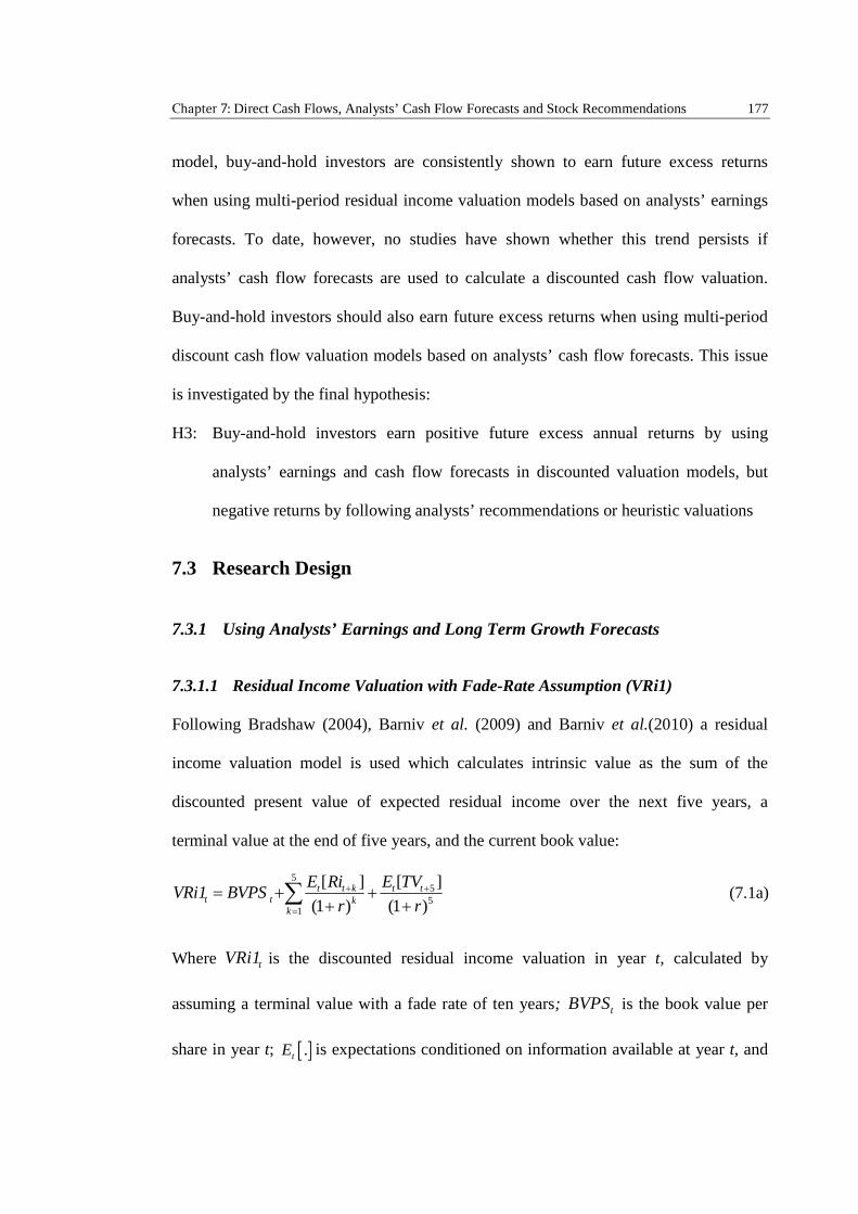
Chapter 7: Direct Cash Flows, Analysts’ Cash Flow Forecasts and Stock Recommendations 177
model, buy-and-hold investors are consistently shown to earn future excess returns
when using multi-period residual income valuation models based on analysts’ earnings
forecasts. To date, however, no studies have shown whether this trend persists if
analysts’ cash flow forecasts are used to calculate a discounted cash flow valuation.
Buy-and-hold investors should also earn future excess returns when using multi-period
discount cash flow valuation models based on analysts’ cash flow forecasts. This issue
is investigated by the final hypothesis:
H3: Buy-and-hold investors earn positive future excess annual returns by using
analysts’ earnings and cash flow forecasts in discounted valuation models, but
negative returns by following analysts’ recommendations or heuristic valuations
7.3 Research Design
7.3.1 Using Analysts’ Earnings and Long Term Growth Forecasts
7.3.1.1 Residual Income Valuation with Fade-Rate Assumption (VRi1)
Following Bradshaw (2004), Barniv et al. (2009) and Barniv et al.(2010) a residual
income valuation model is used which calculates intrinsic value as the sum of the
discounted present value of expected residual income over the next five years, a
terminal value at the end of five years, and the current book value:
555
1
[ ] [ ]
(1 ) (1 )t t k t t
t t kk
E Ri E TVVRi1 BVPS
r r
(7.1a)
Where tVRi1 is the discounted residual income valuation in year t, calculated by
assuming a terminal value with a fade rate of ten years; tBVPS is the book value per
share in year t; .tE is expectations conditioned on information available at year t, and
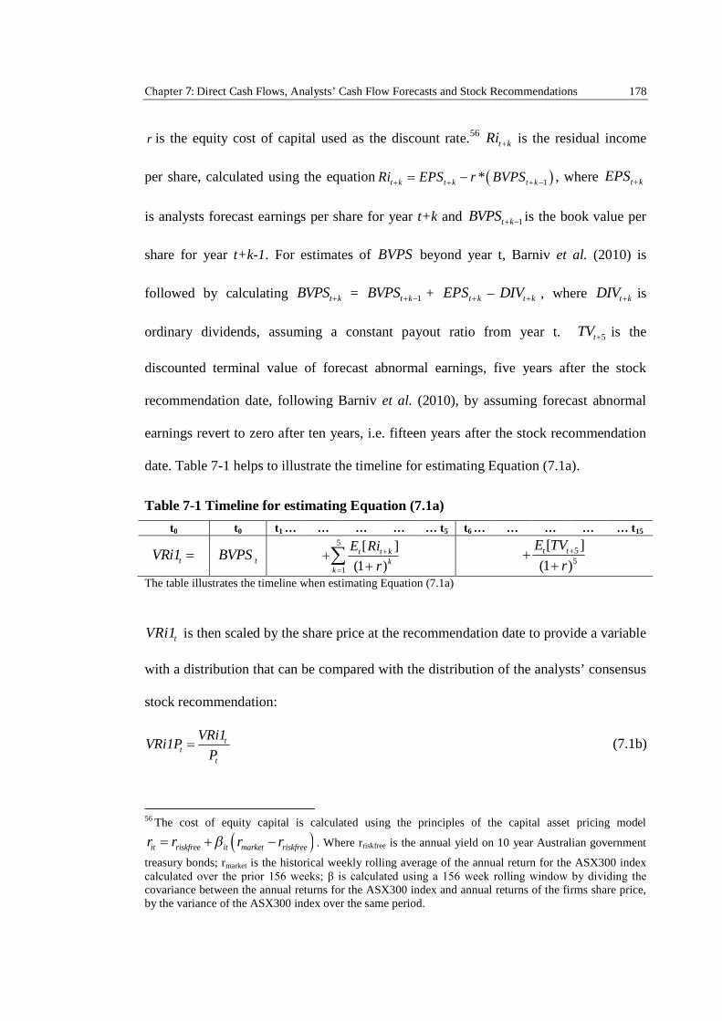
Chapter 7: Direct Cash Flows, Analysts’ Cash Flow Forecasts and Stock Recommendations 178
r is the equity cost of capital used as the discount rate.56t kRi is the residual income
per share, calculated using the equation 1*t k t k t kRi EPS r BVPS , where t kEPS
is analysts forecast earnings per share for year t+k and 1t kBVPS is the book value per
share for year t+k-1. For estimates of BVPS beyond year t, Barniv et al. (2010) is
followed by calculating t kBVPS = 1t kBVPS + t kEPS – t kDIV , where t kDIV is
ordinary dividends, assuming a constant payout ratio from year t. 5tTV is the
discounted terminal value of forecast abnormal earnings, five years after the stock
recommendation date, following Barniv et al. (2010), by assuming forecast abnormal
earnings revert to zero after ten years, i.e. fifteen years after the stock recommendation
date. Table 7-1 helps to illustrate the timeline for estimating Equation (7.1a).
Table 7-1 Timeline for estimating Equation (7.1a)
t0 t0 t1 … … … … … t5 t6 … … … … … t15
tVRi1 tBVPS5
1
[ ]
(1 )t t k
kk
E Ri
r
55
[ ]
(1 )t tE TV
r
The table illustrates the timeline when estimating Equation (7.1a)
tVRi1 is then scaled by the share price at the recommendation date to provide a variable
with a distribution that can be compared with the distribution of the analysts’ consensus
stock recommendation:
tt
t
VRi1VRi1P
P (7.1b)
56 The cost of equity capital is calculated using the principles of the capital asset pricing model
it riskfree it market riskfreer r r r . Where rriskfree is the annual yield on 10 year Australian government
treasury bonds; rmarket is the historical weekly rolling average of the annual return for the ASX300 indexcalculated over the prior 156 weeks; β is calculated using a 156 week rolling window by dividing the covariance between the annual returns for the ASX300 index and annual returns of the firms share price,by the variance of the ASX300 index over the same period.
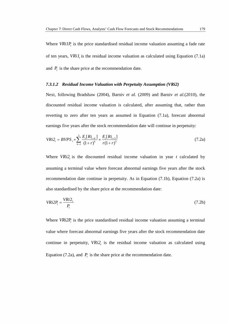
Chapter 7: Direct Cash Flows, Analysts’ Cash Flow Forecasts and Stock Recommendations 179
Where tVRi1P is the price standardised residual income valuation assuming a fade rate
of ten years, tVRi1 is the residual income valuation as calculated using Equation (7.1a)
and tP is the share price at the recommendation date.
7.3.1.2 Residual Income Valuation with Perpetuity Assumption (VRi2)
Next, following Bradshaw (2004), Barniv et al. (2009) and Barniv et al.(2010), the
discounted residual income valuation is calculated, after assuming that, rather than
reverting to zero after ten years as assumed in Equation (7.1a), forecast abnormal
earnings five years after the stock recommendation date will continue in perpetuity:
555
1
[ ] [ ]
(1 ) (1 )t t k t t
t t kk
E Ri E RiVRi2 BVPS
r r r
(7.2a)
Where tVRi2 is the discounted residual income valuation in year t calculated by
assuming a terminal value where forecast abnormal earnings five years after the stock
recommendation date continue in perpetuity. As in Equation (7.1b), Equation (7.2a) is
also standardised by the share price at the recommendation date:
2tt
t
VRiVRi2P
P (7.2b)
Where tVRi2P is the price standardised residual income valuation assuming a terminal
value where forecast abnormal earnings five years after the stock recommendation date
continue in perpetuity, tVRi2 is the residual income valuation as calculated using
Equation (7.2a), and tP is the share price at the recommendation date.
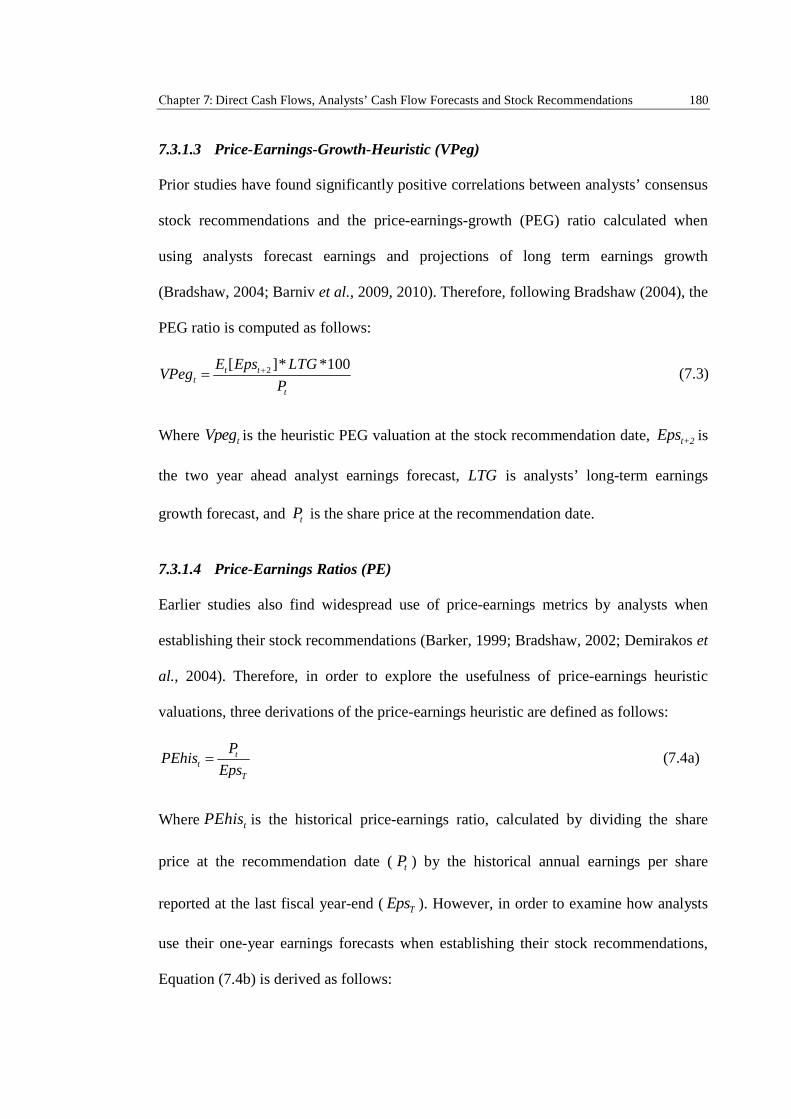
Chapter 7: Direct Cash Flows, Analysts’ Cash Flow Forecasts and Stock Recommendations 180
7.3.1.3 Price-Earnings-Growth-Heuristic (VPeg)
Prior studies have found significantly positive correlations between analysts’ consensus
stock recommendations and the price-earnings-growth (PEG) ratio calculated when
using analysts forecast earnings and projections of long term earnings growth
(Bradshaw, 2004; Barniv et al., 2009, 2010). Therefore, following Bradshaw (2004), the
PEG ratio is computed as follows:
2[ ]* *100t tt
t
E Eps LTGVPeg
P (7.3)
Where tVpeg is the heuristic PEG valuation at the stock recommendation date, t+2Eps is
the two year ahead analyst earnings forecast, LTG is analysts’ long-term earnings
growth forecast, and tP is the share price at the recommendation date.
7.3.1.4 Price-Earnings Ratios (PE)
Earlier studies also find widespread use of price-earnings metrics by analysts when
establishing their stock recommendations (Barker, 1999; Bradshaw, 2002; Demirakos et
al., 2004). Therefore, in order to explore the usefulness of price-earnings heuristic
valuations, three derivations of the price-earnings heuristic are defined as follows:
tt
T
PPEhis
Eps (7.4a)
Where tPEhis is the historical price-earnings ratio, calculated by dividing the share
price at the recommendation date ( tP ) by the historical annual earnings per share
reported at the last fiscal year-end ( TEps ). However, in order to examine how analysts
use their one-year earnings forecasts when establishing their stock recommendations,
Equation (7.4b) is derived as follows:
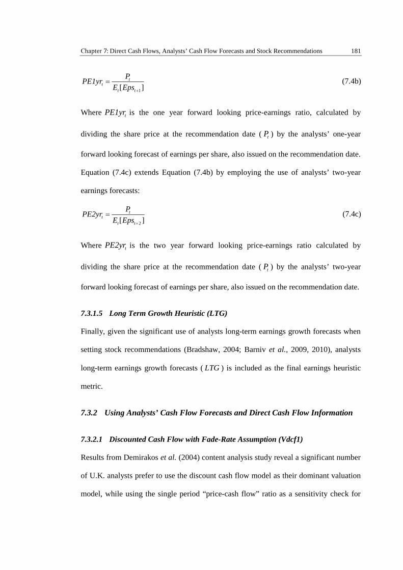
Chapter 7: Direct Cash Flows, Analysts’ Cash Flow Forecasts and Stock Recommendations 181
1[ ]t
t
t t
PPE1yr
E Eps
(7.4b)
Where tPE1yr is the one year forward looking price-earnings ratio, calculated by
dividing the share price at the recommendation date ( tP ) by the analysts’ one-year
forward looking forecast of earnings per share, also issued on the recommendation date.
Equation (7.4c) extends Equation (7.4b) by employing the use of analysts’ two-year
earnings forecasts:
2[ ]t
t
t t
PPE2yr
E Eps
(7.4c)
Where tPE2yr is the two year forward looking price-earnings ratio calculated by
dividing the share price at the recommendation date ( tP ) by the analysts’ two-year
forward looking forecast of earnings per share, also issued on the recommendation date.
7.3.1.5 Long Term Growth Heuristic (LTG)
Finally, given the significant use of analysts long-term earnings growth forecasts when
setting stock recommendations (Bradshaw, 2004; Barniv et al., 2009, 2010), analysts
long-term earnings growth forecasts ( LTG ) is included as the final earnings heuristic
metric.
7.3.2 Using Analysts’ Cash Flow Forecasts and Direct Cash Flow Information
7.3.2.1 Discounted Cash Flow with Fade-Rate Assumption (Vdcf1)
Results from Demirakos et al. (2004) content analysis study reveal a significant number
of U.K. analysts prefer to use the discount cash flow model as their dominant valuation
model, while using the single period “price-cash flow” ratio as a sensitivity check for
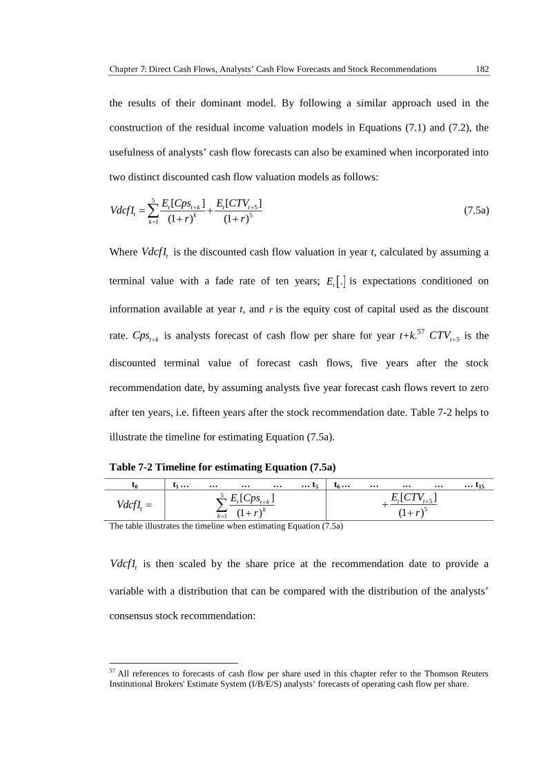
Chapter 7: Direct Cash Flows, Analysts’ Cash Flow Forecasts and Stock Recommendations 182
the results of their dominant model. By following a similar approach used in the
construction of the residual income valuation models in Equations (7.1) and (7.2), the
usefulness of analysts’ cash flow forecasts can also be examined when incorporated into
two distinct discounted cash flow valuation models as follows:
55
51
[ ] [ ]
(1 ) (1 )t t k t t
t kk
E Cps E CTVVdcf1
r r
(7.5a)
Where tVdcf1 is the discounted cash flow valuation in year t, calculated by assuming a
terminal value with a fade rate of ten years; .tE is expectations conditioned on
information available at year t, and r is the equity cost of capital used as the discount
rate. t kCps is analysts forecast of cash flow per share for year t+k.575tCTV is the
discounted terminal value of forecast cash flows, five years after the stock
recommendation date, by assuming analysts five year forecast cash flows revert to zero
after ten years, i.e. fifteen years after the stock recommendation date. Table 7-2 helps to
illustrate the timeline for estimating Equation (7.5a).
Table 7-2 Timeline for estimating Equation (7.5a)
t0 t1 … … … … … t5 t6 … … … … … t15
tVdcf1 5
1
[ ]
(1 )t t k
kk
E Cps
r
5
5
[ ]
(1 )t tE CTV
r
The table illustrates the timeline when estimating Equation (7.5a)
tVdcf1 is then scaled by the share price at the recommendation date to provide a
variable with a distribution that can be compared with the distribution of the analysts’
consensus stock recommendation:
57 All references to forecasts of cash flow per share used in this chapter refer to the Thomson ReutersInstitutional Brokers' Estimate System (I/B/E/S) analysts’ forecasts of operating cash flow per share.
Chapter 7: Direct Cash Flows, Analysts’ Cash Flow Forecasts and Stock Recommendations 183
tt
t
Vdcf1Vdcf1P
P (7.5b)
Where tVdcf1P is the price standardised discounted cash flow valuation assuming a fade
rate of ten years, tVdcf1 is the discounted cash flow valuation as calculated using
Equation (7.5a) and tP is the share price at the recommendation date.
7.3.2.2 Discounted Cash Flow with Perpetuity Assumption (Vdcf2)
Following the approach used for the discounted residual income model in Equation
(7.2a), the discounted cash flow valuation is calculated, after assuming forecast cash
flows, five years after the stock recommendation date, will continue in perpetuity:
k 5
[ ] [ ]
(1+r) r(1+r)
5t t+k t t+5
tk=1
E Cps E CpsVdcf2 = + (7.6a)
Where tVdcf2 is the discounted cash flow valuation in year t calculated by assuming a
terminal value where forecast cash flows five years after the stock recommendation date
continue in perpetuity. As in Equation (7.5b), Equation (7.6a) is also standardised by
the share price at the recommendation date:
tt
t
Vdcf2Vdcf2P =
P(7.6b)
Where tVdcf2P is the price standardised discount cash flow valuation assuming a
terminal value where forecast cash flows five years after the stock recommendation date
continue in perpetuity, tVdcf2 is the discount cash flow valuation as calculated using
Equation (7.6a), and tP is the share price at the recommendation date.
Chapter 7: Direct Cash Flows, Analysts’ Cash Flow Forecasts and Stock Recommendations 184
7.3.2.3 Price-Cash-Flow-Growth Heuristic (VPcshg)
Barniv et al. (2009), Barniv et al. (2010), and Bradshaw (2004) clearly demonstrate the
strong correlation between both the PEG ratio and LTG forecasts and analysts stock
recommendations. It follows, therefore, that by constructing a “price-cash-flow-growth”
metric, the use of analysts’ cash flow forecasts in valuation heuristics to establish their
stock recommendations can be examined:
2[ ]* *100t tt
t
E Cps LTGVPcshg
P (7.7)
Where tVPcshg is the heuristic price-cash-flow-growth valuation at the stock
recommendation date, t+2Cps is the two year ahead analyst cash flow forecast, LTG is
analysts’ long-term earnings growth forecast, and tP is the share price at the
recommendation date.
7.3.2.4 Price-Cash-Flow Ratios (Pcf)
Analysts have also been shown to make use of single period price-cash-flow (PCF)
ratios as a sensitivity check for the results of their dominant valuation model
(Demirakos et al., 2004). Accordingly, three distinct heuristic measures of the PCF are
constructed, considering both historical and forward-looking projections of operating
cash flows:
tt
T
PPcfhis
Cps (7.8a)
Where tPcfhis is the historical price-cash-flow heuristic at the stock recommendation
date, calculated by dividing the share price at the recommendation date ( tP ) by the
historical annual operating cash flow per share reported at the last fiscal year-end
Chapter 7: Direct Cash Flows, Analysts’ Cash Flow Forecasts and Stock Recommendations 185
( TCps ). Equation (7.8b) is then derived to examine how analysts use their one-year cash
flow forecasts when establishing their stock recommendations:
1[ ]t
t
t t
PPcf1yr
E Cps
(7.8b)
Where tPcf1yr is the one year forward looking price-cash-flow ratio, calculated by
dividing the share price at the recommendation date ( tP ) by the analysts’ one-year
forward looking forecast of cash flow per share, also issued on the recommendation
date. Finally, Equation (7.8c) extends Equation (7.8b) by employing the use of analysts’
two-year cash flow forecasts:
2[ ]t
t
t t
PPcf2yr
E Cps
(7.8c)
Where tPcf2yr is the two year forward looking price-cash-flow ratio calculated by
dividing the share price at the recommendation date ( tP ) by the analysts’ two-year
forward looking forecast of cash flow per share, also issued on the recommendation
date.
7.3.2.5 Direct Cash Flow ratio (PDcf)
Cash receipts from customers and payments to suppliers and employees are considered
by analysts to be the most useful information from a direct cash flow statement when
forecasting future cash flows (CFA Institute, 2009). Accordingly, a heuristic measure is
developed to capture whether analyst’s use information from direct cash flow
statements when setting their stock recommendations. This measure is derived by
manipulating the historical price-cash-flow ratio, replacing the denominator with the net
Chapter 7: Direct Cash Flows, Analysts’ Cash Flow Forecasts and Stock Recommendations 186
of the cash receipts from customers per share and payments to suppliers and employees
per share:
( _ )t
t
T
PPDcf
Core OCFps (7.9)
Where tPDcf is the ratio of the share price at the stock recommendation date ( tP ),
divided by core direct cash flows per share _ TCore OCFps as reported at the last
financial year-end. _ TCore OCFps is calculated as the net of cash receipts from
customers and payments to suppliers and employees, standardised by the number of
shares in issue at the last financial year-end.
7.4 Data, Sample and Descriptive Statistics
Using DataStream, 652 firms are initially selected representing companies listed on the
Australian Stock Exchange (ASX) 300 index between the years 2000-2010.58 Monthly
analysts’ stock recommendations and forecasts are then obtained from Thomson
Reuters Institutional Brokers' Estimate System (I/B/E/S) for the entire sample period.
Financial data was obtained from the Aspect Huntley database, which provides a
detailed breakdown of direct operating cash flows that are otherwise unavailable
elsewhere.
Financial and utilities firms, firms with a primary listing other than the ASX, and
firms missing key financial information are then removed from the initial sample.59 A
further 68 firms are removed which have either no analysts’ recommendations or no
58 Australia is historically one of a few countries to mandate the use of direct cash flow statements.Therefore, Australian firms are specifically chosen to examine whether analysts use direct cash flowinformation when issuing their stock recommendations.59 Financial and utility firms are removed because of their different reporting requirements and foreigndomiciled firms are excluded, as they do not follow Australian GAAP.
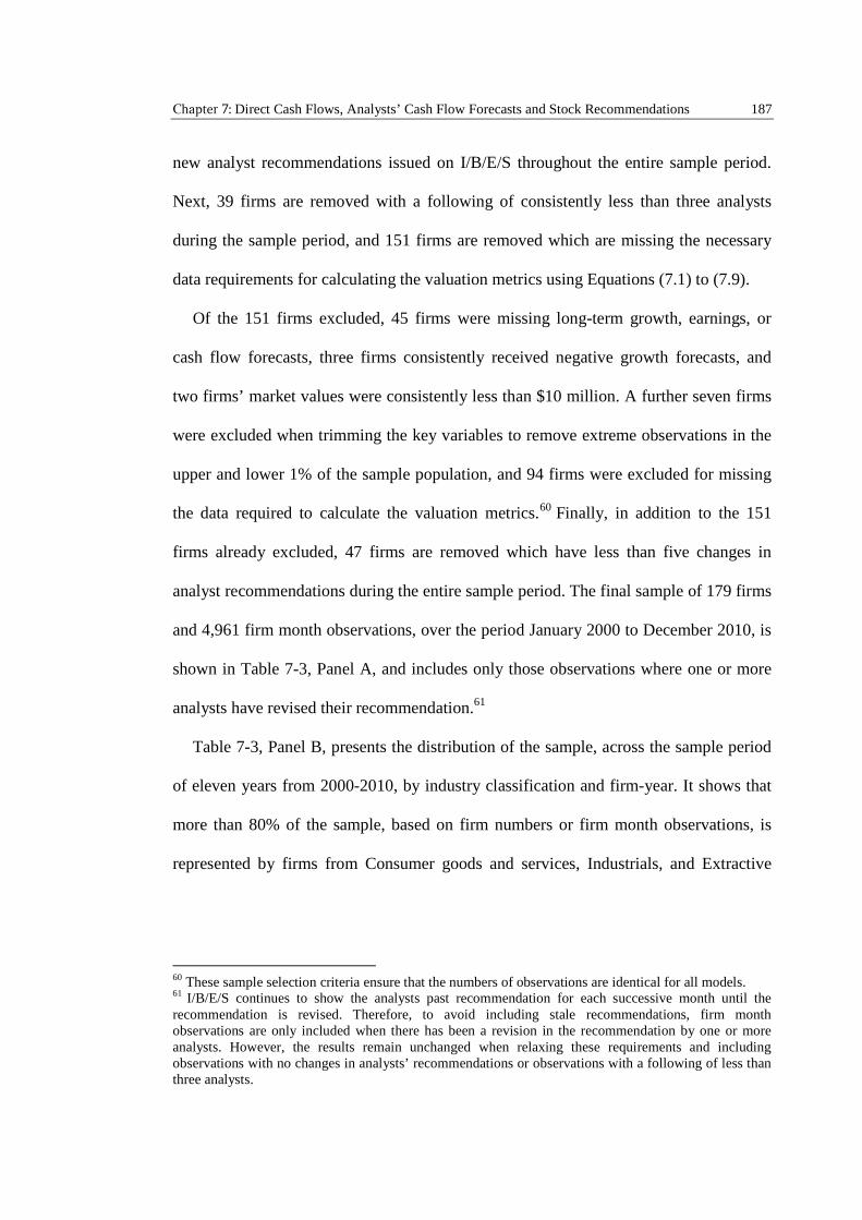
Chapter 7: Direct Cash Flows, Analysts’ Cash Flow Forecasts and Stock Recommendations 187
new analyst recommendations issued on I/B/E/S throughout the entire sample period.
Next, 39 firms are removed with a following of consistently less than three analysts
during the sample period, and 151 firms are removed which are missing the necessary
data requirements for calculating the valuation metrics using Equations (7.1) to (7.9).
Of the 151 firms excluded, 45 firms were missing long-term growth, earnings, or
cash flow forecasts, three firms consistently received negative growth forecasts, and
two firms’ market values were consistently less than $10 million. A further seven firms
were excluded when trimming the key variables to remove extreme observations in the
upper and lower 1% of the sample population, and 94 firms were excluded for missing
the data required to calculate the valuation metrics.60 Finally, in addition to the 151
firms already excluded, 47 firms are removed which have less than five changes in
analyst recommendations during the entire sample period. The final sample of 179 firms
and 4,961 firm month observations, over the period January 2000 to December 2010, is
shown in Table 7-3, Panel A, and includes only those observations where one or more
analysts have revised their recommendation.61
Table 7-3, Panel B, presents the distribution of the sample, across the sample period
of eleven years from 2000-2010, by industry classification and firm-year. It shows that
more than 80% of the sample, based on firm numbers or firm month observations, is
represented by firms from Consumer goods and services, Industrials, and Extractive
60 These sample selection criteria ensure that the numbers of observations are identical for all models.61 I/B/E/S continues to show the analysts past recommendation for each successive month until therecommendation is revised. Therefore, to avoid including stale recommendations, firm monthobservations are only included when there has been a revision in the recommendation by one or moreanalysts. However, the results remain unchanged when relaxing these requirements and includingobservations with no changes in analysts’ recommendations or observations with a following of less thanthree analysts.
Chapter 7: Direct Cash Flows, Analysts’ Cash Flow Forecasts and Stock Recommendations 188
industries.62 Consumer goods and services represent the largest proportion of the sample
population with 2,030 firm month observations. By requiring cost of capital to be
positive, following Hail and Leuz (2003), a drop in the number of observations meeting
the necessary data requirements is further observed during the years 2003, 2009 and
2010 respectively.
Distribution of the sample by the number of recommendations issued at the end of
each of the twelve successive months subsequent to the preceding financial year-end is
shown in Table 7-3, Panel C, with a range from 343 to 465 observations. The highest
numbers of analyst stock recommendations are issued three to four, and eight to nine
months after the financial year-end. This is likely due to the ASX requirements for
companies to publish annual reports within four months, and half-yearly reports within
two months of the reporting date.
62 Prior Australian studies either specifically include or exclude extractive firms from their samples (e.g.,Clinch et al., 2002; Arthur et al., 2010). For the purposes of this study, extractive firms are specificallyincluded. Untabulated findings found that excluding these firms did not significantly change the results.Accordingly, the results presented and discussed in this chapter are based on the sample includingextractive firms.
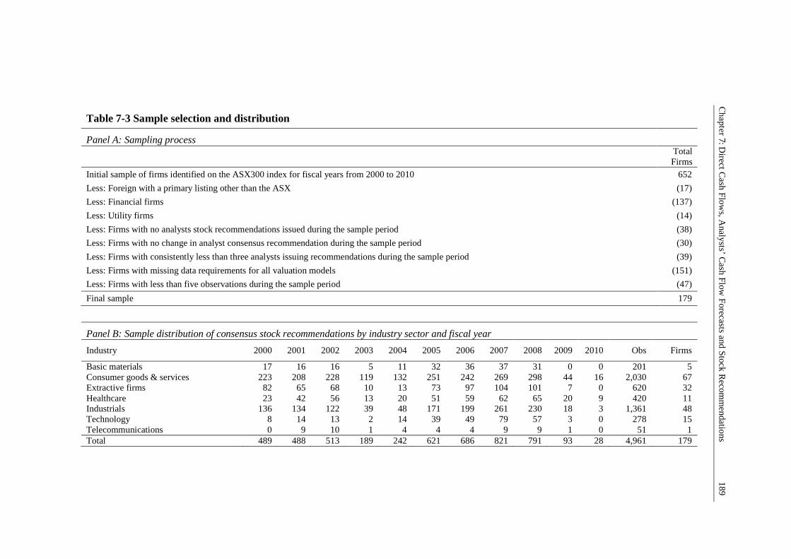
Ch
apter7:D
irectC
ashF
low
s,A
nalysts’C
ashF
lowF
orecastsand
Stock
Recom
mendatio
ns18
9
Table 7-3 Sample selection and distribution
Panel A: Sampling processTotalFirms
Initial sample of firms identified on the ASX300 index for fiscal years from 2000 to 2010 652
Less: Foreign with a primary listing other than the ASX (17)
Less: Financial firms (137)
Less: Utility firms (14)
Less: Firms with no analysts stock recommendations issued during the sample period (38)
Less: Firms with no change in analyst consensus recommendation during the sample period (30)
Less: Firms with consistently less than three analysts issuing recommendations during the sample period (39)
Less: Firms with missing data requirements for all valuation models (151)
Less: Firms with less than five observations during the sample period (47)
Final sample 179
Panel B: Sample distribution of consensus stock recommendations by industry sector and fiscal year
Industry 2000 2001 2002 2003 2004 2005 2006 2007 2008 2009 2010 Obs Firms
Basic materials 17 16 16 5 11 32 36 37 31 0 0 201 5Consumer goods & services 223 208 228 119 132 251 242 269 298 44 16 2,030 67Extractive firms 82 65 68 10 13 73 97 104 101 7 0 620 32Healthcare 23 42 56 13 20 51 59 62 65 20 9 420 11Industrials 136 134 122 39 48 171 199 261 230 18 3 1,361 48Technology 8 14 13 2 14 39 49 79 57 3 0 278 15Telecommunications 0 9 10 1 4 4 4 9 9 1 0 51 1Total 489 488 513 189 242 621 686 821 791 93 28 4,961 179
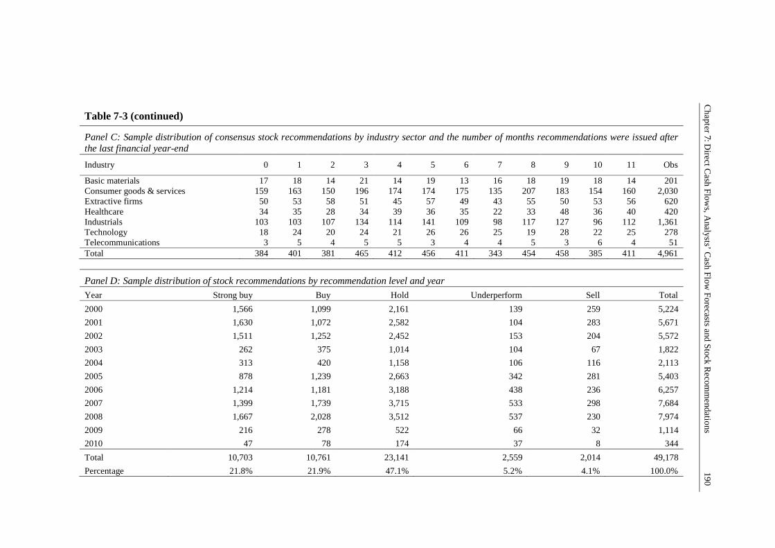
Ch
apter7:D
irectC
ashF
low
s,A
nalysts’C
ashF
lowF
orecastsand
Stock
Recom
mendatio
ns19
0
Table 7-3 (continued)
Panel C: Sample distribution of consensus stock recommendations by industry sector and the number of months recommendations were issued afterthe last financial year-end
Industry 0 1 2 3 4 5 6 7 8 9 10 11 Obs
Basic materials 17 18 14 21 14 19 13 16 18 19 18 14 201Consumer goods & services 159 163 150 196 174 174 175 135 207 183 154 160 2,030Extractive firms 50 53 58 51 45 57 49 43 55 50 53 56 620Healthcare 34 35 28 34 39 36 35 22 33 48 36 40 420Industrials 103 103 107 134 114 141 109 98 117 127 96 112 1,361Technology 18 24 20 24 21 26 26 25 19 28 22 25 278Telecommunications 3 5 4 5 5 3 4 4 5 3 6 4 51Total 384 401 381 465 412 456 411 343 454 458 385 411 4,961
Panel D: Sample distribution of stock recommendations by recommendation level and year
Year Strong buy Buy Hold Underperform Sell Total
2000 1,566 1,099 2,161 139 259 5,224
2001 1,630 1,072 2,582 104 283 5,671
2002 1,511 1,252 2,452 153 204 5,572
2003 262 375 1,014 104 67 1,822
2004 313 420 1,158 106 116 2,113
2005 878 1,239 2,663 342 281 5,403
2006 1,214 1,181 3,188 438 236 6,257
2007 1,399 1,739 3,715 533 298 7,684
2008 1,667 2,028 3,512 537 230 7,974
2009 216 278 522 66 32 1,114
2010 47 78 174 37 8 344
Total 10,703 10,761 23,141 2,559 2,014 49,178
Percentage 21.8% 21.9% 47.1% 5.2% 4.1% 100.0%
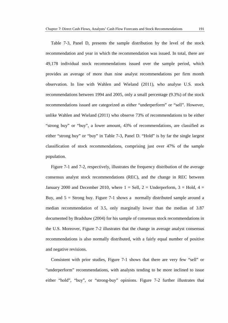
Chapter 7: Direct Cash Flows, Analysts’ Cash Flow Forecasts and Stock Recommendations 191
Table 7-3, Panel D, presents the sample distribution by the level of the stock
recommendation and year in which the recommendation was issued. In total, there are
49,178 individual stock recommendations issued over the sample period, which
provides an average of more than nine analyst recommendations per firm month
observation. In line with Wahlen and Wieland (2011), who analyse U.S. stock
recommendations between 1994 and 2005, only a small percentage (9.3%) of the stock
recommendations issued are categorized as either “underperform” or “sell”. However,
unlike Wahlen and Wieland (2011) who observe 73% of recommendations to be either
“strong buy” or “buy”, a lower amount, 43% of recommendations, are classified as
either “strong buy” or “buy” in Table 7-3, Panel D. “Hold” is by far the single largest
classification of stock recommendations, comprising just over 47% of the sample
population.
Figure 7-1 and 7-2, respectively, illustrates the frequency distribution of the average
consensus analyst stock recommendations (REC), and the change in REC between
January 2000 and December 2010, where 1 = Sell, 2 = Underperform, 3 = Hold, 4 =
Buy, and 5 = Strong buy. Figure 7-1 shows a normally distributed sample around a
median recommendation of 3.5, only marginally lower than the median of 3.87
documented by Bradshaw (2004) for his sample of consensus stock recommendations in
the U.S. Moreover, Figure 7-2 illustrates that the change in average analyst consensus
recommendations is also normally distributed, with a fairly equal number of positive
and negative revisions.
Consistent with prior studies, Figure 7-1 shows that there are very few “sell” or
“underperform” recommendations, with analysts tending to be more inclined to issue
either “hold”, “buy”, or “strong-buy” opinions. Figure 7-2 further illustrates that
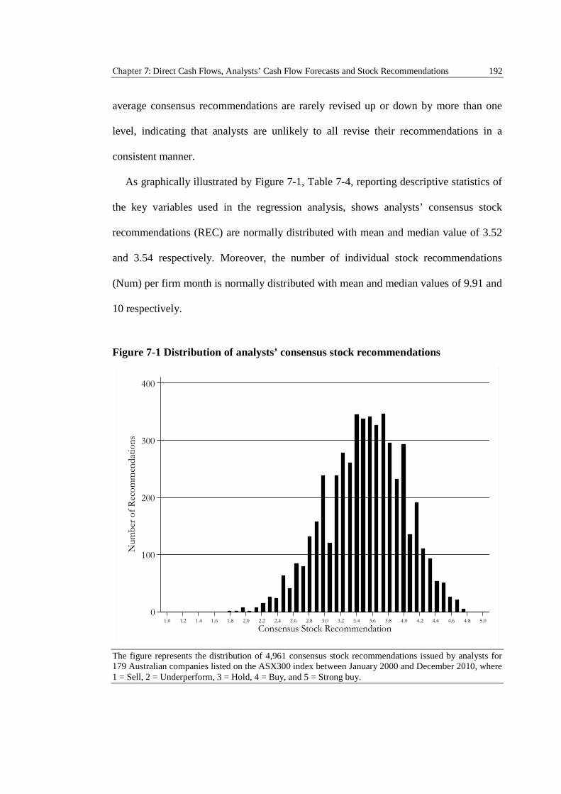
Chapter 7: Direct Cash Flows, Analysts’ Cash Flow Forecasts and Stock Recommendations 192
average consensus recommendations are rarely revised up or down by more than one
level, indicating that analysts are unlikely to all revise their recommendations in a
consistent manner.
As graphically illustrated by Figure 7-1, Table 7-4, reporting descriptive statistics of
the key variables used in the regression analysis, shows analysts’ consensus stock
recommendations (REC) are normally distributed with mean and median value of 3.52
and 3.54 respectively. Moreover, the number of individual stock recommendations
(Num) per firm month is normally distributed with mean and median values of 9.91 and
10 respectively.
Figure 7-1 Distribution of analysts’ consensus stock recommendations
The figure represents the distribution of 4,961 consensus stock recommendations issued by analysts for179 Australian companies listed on the ASX300 index between January 2000 and December 2010, where1 = Sell, 2 = Underperform, 3 = Hold, 4 = Buy, and 5 = Strong buy.
0
100
200
300
400
Num
ber
of
Rec
om
men
dati
ons
1.2 1.4 1.6 1.8 2.2 2.4 2.6 2.8 3.2 3.4 3.6 3.8 4.2 4.4 4.6 4.81.0 2.0 3.0 4.0 5.0
Consensus Stock Recommendation
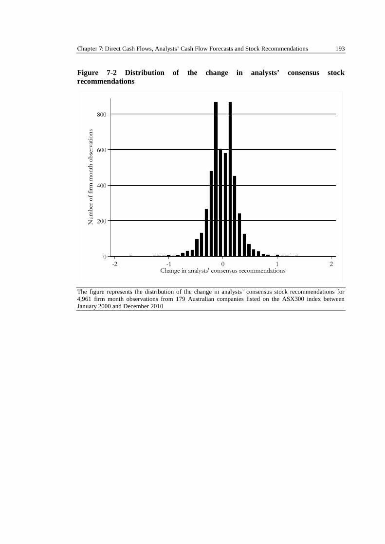
Chapter 7: Direct Cash Flows, Analysts’ Cash Flow Forecasts and Stock Recommendations 193
Figure 7-2 Distribution of the change in analysts’ consensus stockrecommendations
The figure represents the distribution of the change in analysts’ consensus stock recommendations for4,961 firm month observations from 179 Australian companies listed on the ASX300 index betweenJanuary 2000 and December 2010
0
200
400
600
800
Num
ber
of
firm
mo
nth
ob
serv
atio
ns
-2 -1 0 1 2Change in analysts' consensus recommendations
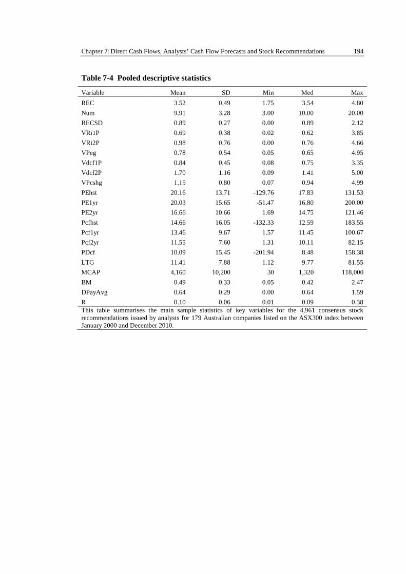
Chapter 7: Direct Cash Flows, Analysts’ Cash Flow Forecasts and Stock Recommendations 194
Table 7-4 Pooled descriptive statistics
Variable Mean SD Min Med Max
REC 3.52 0.49 1.75 3.54 4.80
Num 9.91 3.28 3.00 10.00 20.00
RECSD 0.89 0.27 0.00 0.89 2.12
VRi1P 0.69 0.38 0.02 0.62 3.85
VRi2P 0.98 0.76 0.00 0.76 4.66
VPeg 0.78 0.54 0.05 0.65 4.95
Vdcf1P 0.84 0.45 0.08 0.75 3.35
Vdcf2P 1.70 1.16 0.09 1.41 5.00
VPcshg 1.15 0.80 0.07 0.94 4.99
PEhst 20.16 13.71 -129.76 17.83 131.53
PE1yr 20.03 15.65 -51.47 16.80 200.00
PE2yr 16.66 10.66 1.69 14.75 121.46
Pcfhst 14.66 16.05 -132.33 12.59 183.55
Pcf1yr 13.46 9.67 1.57 11.45 100.67
Pcf2yr 11.55 7.60 1.31 10.11 82.15
PDcf 10.09 15.45 -201.94 8.48 158.38
LTG 11.41 7.88 1.12 9.77 81.55
MCAP 4,160 10,200 30 1,320 118,000
BM 0.49 0.33 0.05 0.42 2.47
DPayAvg 0.64 0.29 0.00 0.64 1.59
R 0.10 0.06 0.01 0.09 0.38This table summarises the main sample statistics of key variables for the 4,961 consensus stockrecommendations issued by analysts for 179 Australian companies listed on the ASX300 index betweenJanuary 2000 and December 2010.
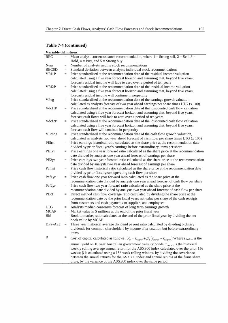
Chapter 7: Direct Cash Flows, Analysts’ Cash Flow Forecasts and Stock Recommendations 195
Table 7-4 (continued)
Variable definitions:REC = Mean analyst consensus stock recommendation, where 1 = Strong sell, 2 = Sell, 3 =
Hold, 4 = Buy, and 5 = Strong buyNum = Number of analysts issuing stock recommendationsRECSD = Standard deviation between analysts individual stock recommendationsVRi1P = Price standardised at the recommendation date of the residual income valuation
calculated using a five year forecast horizon and assuming that, beyond five years,forecast residual income will fade to zero over a period of ten years
VRi2P = Price standardised at the recommendation date of the residual income valuationcalculated using a five year forecast horizon and assuming that, beyond five years,forecast residual income will continue in perpetuity
VPeg = Price standardised at the recommendation date of the earnings growth valuation,calculated as analysts forecast of two year ahead earnings per share times LTG (x 100)
Vdcf1P = Price standardised at the recommendation date of the discounted cash flow valuationcalculated using a five year forecast horizon and assuming that, beyond five years,forecast cash flows will fade to zero over a period of ten years
Vdcf2P = Price standardised at the recommendation date of the discounted cash flow valuationcalculated using a five year forecast horizon and assuming that, beyond five years,forecast cash flow will continue in perpetuity
VPcshg = Price standardised at the recommendation date of the cash flow growth valuation,calculated as analysts two year ahead forecast of cash flow per share times LTG (x 100)
PEhst = Price earnings historical ratio calculated as the share price at the recommendation datedivided by prior fiscal year’s earnings before extraordinary items per share
PE1yr = Price earnings one year forward ratio calculated as the share price at the recommendationdate divided by analysts one year ahead forecast of earnings per share
PE2yr = Price earnings two year forward ratio calculated as the share price at the recommendationdate divided by analysts two year ahead forecast of earnings per share
Pcfhst = Price cash flow historical ratio calculated as the share price at the recommendation datedivided by prior fiscal years operating cash flow per share
Pcf1yr = Price cash flow one year forward ratio calculated as the share price at therecommendation date divided by analysts one year ahead forecast of cash flow per share
Pcf2yr = Price cash flow two year forward ratio calculated as the share price at therecommendation date divided by analysts two year ahead forecast of cash flow per share
PDcf = Direct method cash flow coverage ratio calculated by dividing the share price at therecommendation date by the prior fiscal years net value per share of the cash receiptsfrom customers and cash payments to suppliers and employees
LTG = Analysts median consensus forecast of long term earnings growthMCAP = Market value in $ millions at the end of the prior fiscal yearBM = Book to market ratio calculated at the end of the prior fiscal year by dividing the net
book value by MCAPDPayAvg = Three year historical average dividend payout ratio calculated by dividing ordinary
dividends for common shareholders by income after taxation but before extraordinaryitems
R = Cost of capital calculated as follows: it riskfree it market riskfreeR r r r Where rriskfree is the
annual yield on 10 year Australian government treasury bonds; rmarket is the historicalweekly rolling average annual return for the ASX300 index calculated over the prior 156weeks; β is calculated using a 156 week rolling window by dividing the covariance between the annual returns for the ASX300 index and annual returns of the firms shareprice, by the variance of the ASX300 index over the same period.
Chapter 7: Direct Cash Flows, Analysts’ Cash Flow Forecasts and Stock Recommendations 196
The minimum number of analysts issuing a stock recommendation for a given firm
month is three analysts, due to the sample restriction limiting observations to include
only those firm months with a minimum of three analysts63. Num further shows there
are no more than 20 analysts issuing stock recommendations for any given firm month.
The low average and median standard deviation between analysts’ individual stock
recommendations (RECSD) of 0.89 implies a high level of consensus between analyst
recommendations.
For all the price standardised valuation metrics, a value of “1” would imply that the
current share price is equal to the estimated valuation measure and would therefore
expect a “hold” recommendation. Likewise, if the valuation metric were below/above 1,
a “sell”/“buy” recommendation would be expected. The price standardised residual
income models (VRi1P) and (VRi2P) have mean values of 0.69 and 0.98 respectively,
compared with those reported by Barniv et al. (2010) of 0.69 and 0.82 for their sample
of high investor participation countries from 1993-2007.64 Respective mean values of
the discounted cash flow models Vdcf1P and Vdcf2P of 0.84 and 1.70, and the price-
cash-flow growth model (VPcshg) of 1.15, are all larger than the price standardised
earnings metrics. Figure 7-3 to Figure 7-6 graphically displays the distribution of VRi1P,
VRi2P, Vdcf1P, and Vdcf2P respectively, and illustrates the difference between using a
terminal valuation in Figure 7-4 and Figure 7-6, and a fade rate assumption in Figure
7-3 and Figure 7-5. They also illustrate that the discounted cash flow valuation methods
63 While all the models are estimated using observations with three or more analysts issuing stockrecommendations, the results are materially consistent when relaxing this requirement and including allobservations with less than three analysts issuing stock recommendations.64 Following Bradshaw (2004), observations with values below 0 or above 5 are excluded for the residualincome valuation metrics (VRi1P) and (VRi2P), and price-earnings-growth valuation metric (VPeg).Moreover, observations with values below 0 or above 5 are also excluded for the discounted cash flowvaluation metrics (Vdcf1P) and (Vdcf2P), and the price-cash-flow-growth valuation metric (VPcshg).
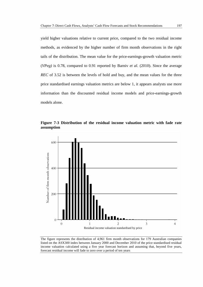
Chapter 7: Direct Cash Flows, Analysts’ Cash Flow Forecasts and Stock Recommendations 197
yield higher valuations relative to current price, compared to the two residual income
methods, as evidenced by the higher number of firm month observations in the right
tails of the distribution. The mean value for the price-earnings-growth valuation metric
(VPeg) is 0.78, compared to 0.91 reported by Barniv et al. (2010). Since the average
REC of 3.52 is between the levels of hold and buy, and the mean values for the three
price standardised earnings valuation metrics are below 1, it appears analysts use more
information than the discounted residual income models and price-earnings-growth
models alone.
Figure 7-3 Distribution of the residual income valuation metric with fade rateassumption
The figure represents the distribution of 4,961 firm month observations for 179 Australian companieslisted on the ASX300 index between January 2000 and December 2010 of the price standardised residualincome valuation calculated using a five year forecast horizon and assuming that, beyond five years,forecast residual income will fade to zero over a period of ten years
0
200
400
600
Num
ber
of
firm
mon
thob
serv
atio
ns
0 1 2 3 4Residual income valuation standardized by priceResidual income valuation standardised by price
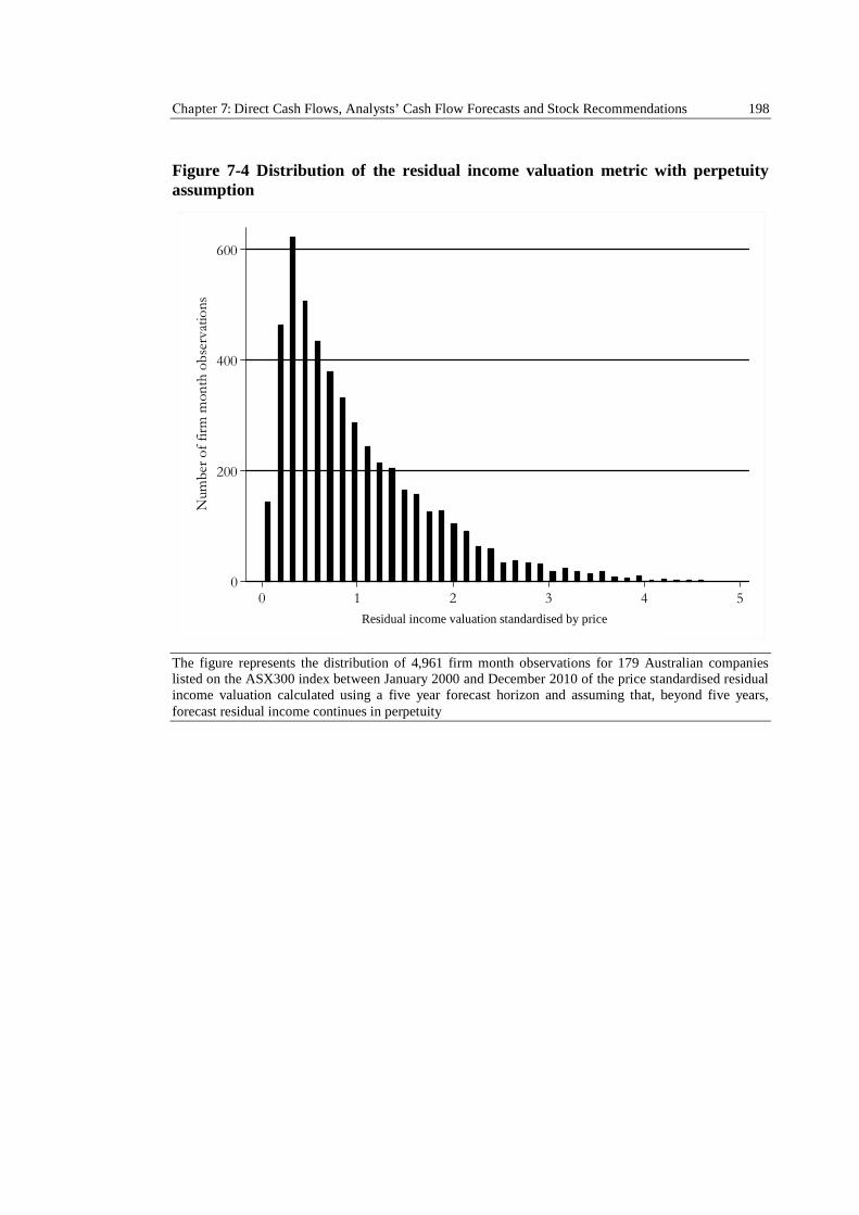
Chapter 7: Direct Cash Flows, Analysts’ Cash Flow Forecasts and Stock Recommendations 198
Figure 7-4 Distribution of the residual income valuation metric with perpetuityassumption
The figure represents the distribution of 4,961 firm month observations for 179 Australian companieslisted on the ASX300 index between January 2000 and December 2010 of the price standardised residualincome valuation calculated using a five year forecast horizon and assuming that, beyond five years,forecast residual income continues in perpetuity
0
200
400
600
Num
ber
of
firm
mo
nth
obse
rvat
ion
s
0 1 2 3 4 5Residual income valuation standardized by priceResidual income valuation standardised by price
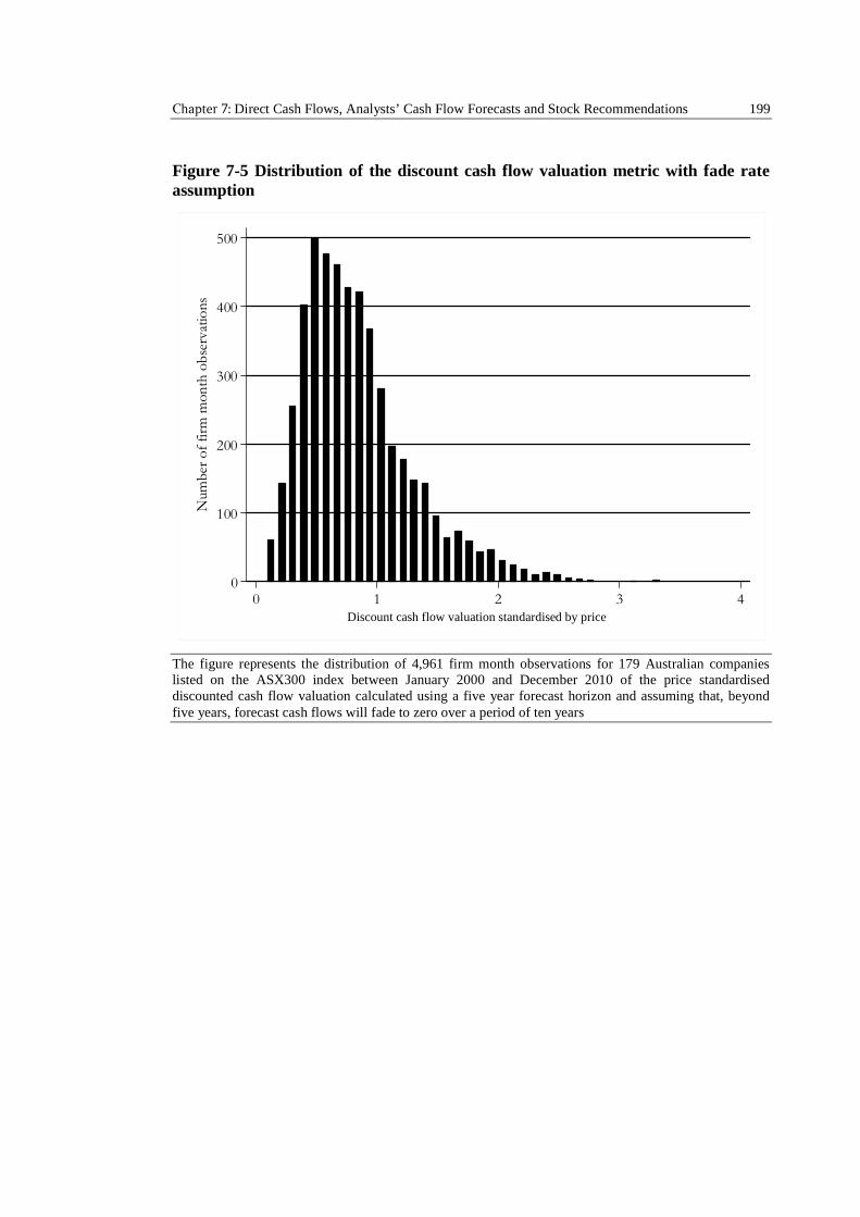
Chapter 7: Direct Cash Flows, Analysts’ Cash Flow Forecasts and Stock Recommendations 199
Figure 7-5 Distribution of the discount cash flow valuation metric with fade rateassumption
The figure represents the distribution of 4,961 firm month observations for 179 Australian companieslisted on the ASX300 index between January 2000 and December 2010 of the price standardiseddiscounted cash flow valuation calculated using a five year forecast horizon and assuming that, beyondfive years, forecast cash flows will fade to zero over a period of ten years
0
100
200
300
400
500
Num
ber
of
firm
mo
nth
obse
rvat
ion
s
0 1 2 3 4Discount cash flow valuation standardized by priceDiscount cash flow valuation standardised by price
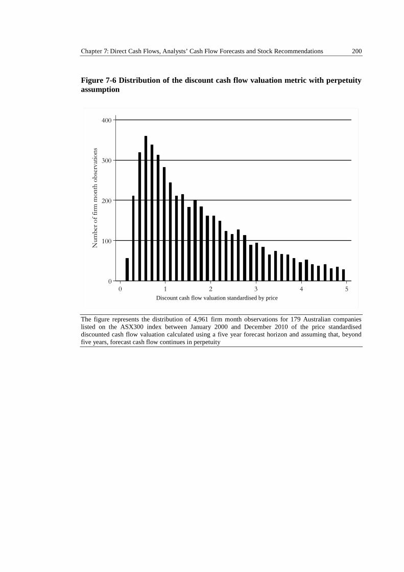
Chapter 7: Direct Cash Flows, Analysts’ Cash Flow Forecasts and Stock Recommendations 200
Figure 7-6 Distribution of the discount cash flow valuation metric with perpetuityassumption
The figure represents the distribution of 4,961 firm month observations for 179 Australian companieslisted on the ASX300 index between January 2000 and December 2010 of the price standardiseddiscounted cash flow valuation calculated using a five year forecast horizon and assuming that, beyondfive years, forecast cash flow continues in perpetuity
0
100
200
300
400
Num
ber
of
firm
mo
nth
obse
rvat
ion
s
0 1 2 3 4 5Discount cash flow valuation standardized by priceDiscount cash flow valuation standardised by price
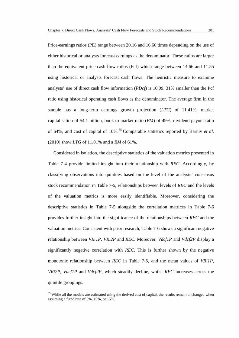
Chapter 7: Direct Cash Flows, Analysts’ Cash Flow Forecasts and Stock Recommendations 201
Price-earnings ratios (PE) range between 20.16 and 16.66 times depending on the use of
either historical or analysts forecast earnings as the denominator. These ratios are larger
than the equivalent price-cash-flow ratios (Pcf) which range between 14.66 and 11.55
using historical or analysts forecast cash flows. The heuristic measure to examine
analysts’ use of direct cash flow information (PDcf) is 10.09, 31% smaller than the Pcf
ratio using historical operating cash flows as the denominator. The average firm in the
sample has a long-term earnings growth projection (LTG) of 11.41%, market
capitalisation of $4.1 billion, book to market ratio (BM) of 49%, dividend payout ratio
of 64%, and cost of capital of 10%.65 Comparable statistics reported by Barniv et al.
(2010) show LTG of 11.01% and a BM of 61%.
Considered in isolation, the descriptive statistics of the valuation metrics presented in
Table 7-4 provide limited insight into their relationship with REC. Accordingly, by
classifying observations into quintiles based on the level of the analysts’ consensus
stock recommendation in Table 7-5, relationships between levels of REC and the levels
of the valuation metrics is more easily identifiable. Moreover, considering the
descriptive statistics in Table 7-5 alongside the correlation matrices in Table 7-6
provides further insight into the significance of the relationships between REC and the
valuation metrics. Consistent with prior research, Table 7-6 shows a significant negative
relationship between VRi1P, VRi2P and REC. Moreover, Vdcf1P and Vdcf2P display a
significantly negative correlation with REC. This is further shown by the negative
monotonic relationship between REC in Table 7-5, and the mean values of VRi1P,
VRi2P, Vdcf1P and Vdcf2P, which steadily decline, whilst REC increases across the
quintile groupings.
65 While all the models are estimated using the derived cost of capital, the results remain unchanged whenassuming a fixed rate of 5%, 10%, or 15%.
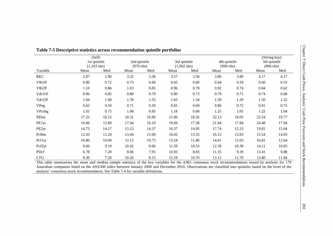
Ch
apter7:D
irectC
ashF
low
s,A
nalysts’C
ashF
lowF
orecastsand
Stock
Recom
mendatio
ns20
2
Table 7-5 Descriptive statistics across recommendation quintile portfolios
(Sell)1st quintile(1,103 obs)
2nd quintile(970 obs)
3rd quintile(1,002 obs)
4th quintile(990 obs)
(Strong buy)5th quintile(896 obs)
Variable Mean Med Mean Med Mean Med Mean Med Mean Med
REC 2.87 2.90 3.32 3.30 3.57 3.56 3.80 3.80 4.17 4.17
VRi1P 0.80 0.72 0.73 0.66 0.65 0.60 0.64 0.59 0.60 0.53
VRi2P 1.10 0.86 1.03 0.83 0.96 0.78 0.92 0.74 0.84 0.62
Vdcf1P 0.96 0.85 0.88 0.79 0.80 0.73 0.79 0.71 0.74 0.68
Vdcf2P 1.94 1.68 1.78 1.55 1.65 1.34 1.59 1.29 1.50 1.22
VPeg 0.62 0.50 0.71 0.59 0.81 0.69 0.86 0.72 0.91 0.75
VPcshg 1.01 0.75 1.08 0.85 1.18 0.98 1.25 1.05 1.25 1.04
PEhst 17.25 16.12 18.31 16.96 21.06 18.56 22.13 19.05 22.54 19.77
PE1yr 16.86 15.89 17.94 16.10 19.69 17.38 21.94 17.84 24.48 17.94
PE2yr 14.73 14.17 15.13 14.37 16.37 14.95 17.74 15.33 19.82 15.04
Pcfhst 12.43 11.24 13.44 11.69 16.02 13.33 16.15 13.83 15.54 14.03
Pcf1yr 10.80 10.09 12.15 10.75 13.54 11.80 14.61 12.03 16.81 12.64
Pcf2yr 9.66 9.19 10.42 9.60 11.59 10.53 12.39 10.38 14.11 10.83
PDcf 6.78 7.20 8.66 7.95 10.93 8.83 11.35 9.39 13.41 9.88
LTG 8.30 7.20 10.20 8.15 12.19 10.70 13.12 11.70 13.80 11.84This table summarises the mean and median sample statistics of the key variables for the 4,961 consensus stock recommendations issued by analysts for 179Australian companies listed on the ASX300 index between January 2000 and December 2010. Observations are classified into quintiles based on the level of theanalysts’ consensus stock recommendation. See Table 7-4 for variable definitions.
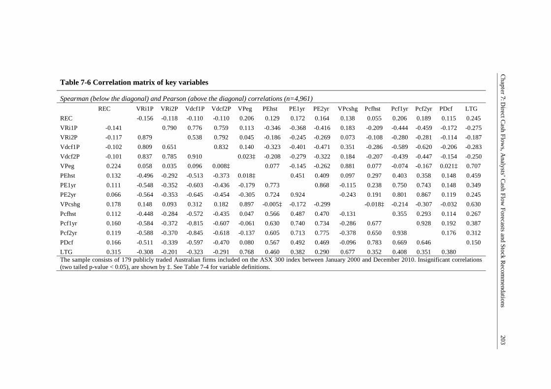
Ch
apter7:D
irectC
ashF
low
s,A
nalysts’C
ashF
lowF
orecastsand
Stock
Recom
mendatio
ns20
3
Table 7-6 Correlation matrix of key variables
Spearman (below the diagonal) and Pearson (above the diagonal) correlations (n=4,961)
REC VRi1P VRi2P Vdcf1P Vdcf2P VPeg PEhst PE1yr PE2yr VPcshg Pcfhst Pcf1yr Pcf2yr PDcf LTG
REC -0.156 -0.118 -0.110 -0.110 0.206 0.129 0.172 0.164 0.138 0.055 0.206 0.189 0.115 0.245
VRi1P -0.141 0.790 0.776 0.759 0.113 -0.346 -0.368 -0.416 0.183 -0.209 -0.444 -0.459 -0.172 -0.275
VRi2P -0.117 0.879 0.538 0.792 0.045 -0.186 -0.245 -0.269 0.073 -0.108 -0.280 -0.281 -0.114 -0.187
Vdcf1P -0.102 0.809 0.651 0.832 0.140 -0.323 -0.401 -0.471 0.351 -0.286 -0.589 -0.620 -0.206 -0.283
Vdcf2P -0.101 0.837 0.785 0.910 0.023‡ -0.208 -0.279 -0.322 0.184 -0.207 -0.439 -0.447 -0.154 -0.250
VPeg 0.224 0.058 0.035 0.096 0.008‡ 0.077 -0.145 -0.262 0.881 0.077 -0.074 -0.167 0.021‡ 0.707
PEhst 0.132 -0.496 -0.292 -0.513 -0.373 0.018‡ 0.451 0.409 0.097 0.297 0.403 0.358 0.148 0.459
PE1yr 0.111 -0.548 -0.352 -0.603 -0.436 -0.179 0.773 0.868 -0.115 0.238 0.750 0.743 0.148 0.349
PE2yr 0.066 -0.564 -0.353 -0.645 -0.454 -0.305 0.724 0.924 -0.243 0.191 0.801 0.867 0.119 0.245
VPcshg 0.178 0.148 0.093 0.312 0.182 0.897 -0.005‡ -0.172 -0.299 -0.018‡ -0.214 -0.307 -0.032 0.630
Pcfhst 0.112 -0.448 -0.284 -0.572 -0.435 0.047 0.566 0.487 0.470 -0.131 0.355 0.293 0.114 0.267
Pcf1yr 0.160 -0.584 -0.372 -0.815 -0.607 -0.061 0.630 0.740 0.734 -0.286 0.677 0.928 0.192 0.387
Pcf2yr 0.119 -0.588 -0.370 -0.845 -0.618 -0.137 0.605 0.713 0.775 -0.378 0.650 0.938 0.176 0.312
PDcf 0.166 -0.511 -0.339 -0.597 -0.470 0.080 0.567 0.492 0.469 -0.096 0.783 0.669 0.646 0.150
LTG 0.315 -0.308 -0.201 -0.323 -0.291 0.768 0.460 0.382 0.290 0.677 0.352 0.408 0.351 0.380The sample consists of 179 publicly traded Australian firms included on the ASX 300 index between January 2000 and December 2010. Insignificant correlations(two tailed p-value < 0.05), are shown by ‡. See Table 7-4 for variable definitions.
Chapter 7: Direct Cash Flows, Analysts’ Cash Flow Forecasts and Stock Recommendations 204
Analysts appear to disregard the results of multi-period valuations, by issuing
counterintuitive more/less favourable recommendations for stocks with low/high
valuations compared to the current share price, providing initial confirmation of H2.
In contrast, however, the heuristic measures display a significantly positive
correlation with REC in Table 7-6, along with monotonically positive relationships in
Table 7-5, except Pcfhst, which, after increasing monotonically through the first four
quintiles, falls in the fifth. These descriptive statistics provide initial evidence in support
of H1 that analysts predominantly employ valuation heuristics when recommending
stocks. Analysts forecast of long-term earnings growth (LTG) displays the highest
positive correlation with REC of 31.5%, consistent with prior studies, and further
emphasising the importance placed on LTG by analysts when issuing their
recommendations. Moreover, Table 7-5 displays LTG growing monotonically from
8.3% at the lowest recommendation levels, up to 13.8% at the highest recommendation
levels. VPeg and VPcshg display the second and third highest positive correlations with
REC of 22.4% and 17.8%, likely driven by the incorporation of LTG within the models.
PDcf and Pcf1yr are the last two heuristic measures that are correlated with REC at a
level greater than 15%, providing initial evidence of the importance given by analysts to
historical direct cash flows and their cash flow forecasts when recommending stocks.
Between the three PE ratios, the historical PE ratio is most highly correlated with REC
at 13.2%. By comparison, however, between the three Pcf ratios, the ratio utilising
analysts one year cash flow forecast yields the highest correlation with REC of 16%.
When recommending stocks, analysts appear to place more reliance on historical
earnings and estimates of future cash flows, rather than historical cash flows and
estimates of future earnings.
Chapter 7: Direct Cash Flows, Analysts’ Cash Flow Forecasts and Stock Recommendations 205
7.5 Regression Results
Firm level fixed effects regressions are used to test the relationship between analysts’
consensus stock recommendations and the valuation and heuristic measures calculated
from Equations (7.1) to (7.9).66 Moreover, while suppressed from the tabulated results,
all the models include controls for the industry classification, year, and the number of
months prior to the next financial year, in which the stock recommendation was issued.
Standard errors are adjusted for firm level clustering, and are robust to
heteroskedasticity and autocorrelation. Following Bradshaw (2004), Barniv et al.
(2009), and Barniv et al. (2010), all the regressions are estimated by using the quintile
rankings of valuation estimates as explanatory variables, which are scaled to range
between 0 and 1 (e.g. (Quintile-1)/4). 67 Vuong tests are then used to compare the
relative explanatory power between the different models (Bradshaw, 2004).
7.5.1 Analysis of Analysts’ Recommendations on Valuation Metrics
The initial analysis, reported in Table 7-7 to Table 7-8, follow Bradshaw (2004), by
regressing analysts’ consensus stock recommendations on the quintile rankings of each
multi-period valuation and heuristic model (VM), calculated using Equations (7.1) to
(7.9), as follows:
0 1 2REC VM Controls FE (7.10)
66 Untabulated results, of Hausman’s (1978) specification test, rejected the null hypothesis of there beingno systematic difference between the coefficients of the firm level random effects, and firm level fixedeffects models. Accordingly, the firm fixed effects model is chosen as the more efficient estimator of thebeta coefficients.67 While all the models are estimated using quintile rankings of the independent variables, there is nomaterial effect on any inferences by using the actual, rather than ranked, values for the independentvariables.
Chapter 7: Direct Cash Flows, Analysts’ Cash Flow Forecasts and Stock Recommendations 206
Where REC is the analyst average consensus recommendation, VM is the valuation or
heuristic model calculated using Equations (7.1) to (7.9), FE are firm level fixed
effects, and Controls include controls for the industry classification, year, and the
number of months prior to the next financial year, in which the stock recommendation
was issued.
Regression results of Equation (7.10) are presented in two tables, testing hypotheses
H1 and H2. Table 7-7 display the results of multi-period valuation and heuristic models
using analysts forecast earnings, historical earnings, and long-term earnings growth
forecasts. Meanwhile, Table 7-8 presents the findings from multi-period valuation and
heuristic models using analysts forecast cash flows, historical net cash flows, and
historical core direct cash flows. Results in Table 7-7 show a significant negative
coefficient for VRi1P, and no significant relationship between REC and VRi2P,
providing supporting evidence for H2. In contrast, with the exception of the coefficient
for PE2yr, which is insignificant, all the earnings based heuristic models are related
positively, and significantly, to analysts’ average consensus recommendation. Moreover,
between all the earnings based valuation models, LTG has the highest coefficient of
0.271 and R2 of 18.5%.
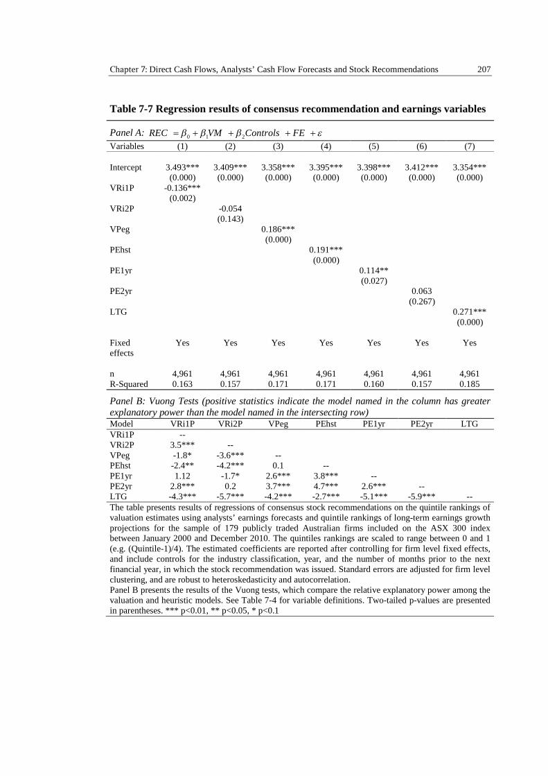
Chapter 7: Direct Cash Flows, Analysts’ Cash Flow Forecasts and Stock Recommendations 207
Table 7-7 Regression results of consensus recommendation and earnings variables
Panel A: 0 1 2REC VM Controls FE
Variables (1) (2) (3) (4) (5) (6) (7)
Intercept 3.493*** 3.409*** 3.358*** 3.395*** 3.398*** 3.412*** 3.354***(0.000) (0.000) (0.000) (0.000) (0.000) (0.000) (0.000)
VRi1P -0.136***(0.002)
VRi2P -0.054(0.143)
VPeg 0.186***(0.000)
PEhst 0.191***(0.000)
PE1yr 0.114**(0.027)
PE2yr 0.063(0.267)
LTG 0.271***(0.000)
Fixedeffects
Yes Yes Yes Yes Yes Yes Yes
n 4,961 4,961 4,961 4,961 4,961 4,961 4,961R-Squared 0.163 0.157 0.171 0.171 0.160 0.157 0.185
Panel B: Vuong Tests (positive statistics indicate the model named in the column has greaterexplanatory power than the model named in the intersecting row)Model VRi1P VRi2P VPeg PEhst PE1yr PE2yr LTGVRi1P --VRi2P 3.5*** --VPeg -1.8* -3.6*** --PEhst -2.4** -4.2*** 0.1 --PE1yr 1.12 -1.7* 2.6*** 3.8*** --PE2yr 2.8*** 0.2 3.7*** 4.7*** 2.6*** --LTG -4.3*** -5.7*** -4.2*** -2.7*** -5.1*** -5.9*** --The table presents results of regressions of consensus stock recommendations on the quintile rankings ofvaluation estimates using analysts’ earnings forecasts and quintile rankings of long-term earnings growthprojections for the sample of 179 publicly traded Australian firms included on the ASX 300 indexbetween January 2000 and December 2010. The quintiles rankings are scaled to range between 0 and 1(e.g. (Quintile-1)/4). The estimated coefficients are reported after controlling for firm level fixed effects,and include controls for the industry classification, year, and the number of months prior to the nextfinancial year, in which the stock recommendation was issued. Standard errors are adjusted for firm levelclustering, and are robust to heteroskedasticity and autocorrelation.Panel B presents the results of the Vuong tests, which compare the relative explanatory power among thevaluation and heuristic models. See Table 7-4 for variable definitions. Two-tailed p-values are presentedin parentheses. *** p<0.01, ** p<0.05, * p<0.1
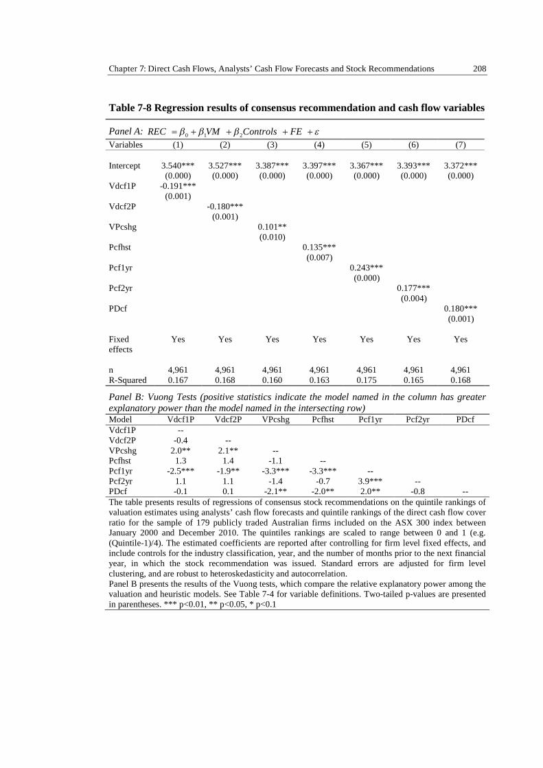
Chapter 7: Direct Cash Flows, Analysts’ Cash Flow Forecasts and Stock Recommendations 208
Table 7-8 Regression results of consensus recommendation and cash flow variables
Panel A: 0 1 2REC VM Controls FE
Variables (1) (2) (3) (4) (5) (6) (7)
Intercept 3.540*** 3.527*** 3.387*** 3.397*** 3.367*** 3.393*** 3.372***(0.000) (0.000) (0.000) (0.000) (0.000) (0.000) (0.000)
Vdcf1P -0.191***(0.001)
Vdcf2P -0.180***(0.001)
VPcshg 0.101**(0.010)
Pcfhst 0.135***(0.007)
Pcf1yr 0.243***(0.000)
Pcf2yr 0.177***(0.004)
PDcf 0.180***(0.001)
Fixedeffects
Yes Yes Yes Yes Yes Yes Yes
n 4,961 4,961 4,961 4,961 4,961 4,961 4,961R-Squared 0.167 0.168 0.160 0.163 0.175 0.165 0.168
Panel B: Vuong Tests (positive statistics indicate the model named in the column has greaterexplanatory power than the model named in the intersecting row)Model Vdcf1P Vdcf2P VPcshg Pcfhst Pcf1yr Pcf2yr PDcfVdcf1P --Vdcf2P -0.4 --VPcshg 2.0** 2.1** --Pcfhst 1.3 1.4 -1.1 --Pcf1yr -2.5*** -1.9** -3.3*** -3.3*** --Pcf2yr 1.1 1.1 -1.4 -0.7 3.9*** --PDcf -0.1 0.1 -2.1** -2.0** 2.0** -0.8 --The table presents results of regressions of consensus stock recommendations on the quintile rankings ofvaluation estimates using analysts’ cash flow forecasts and quintile rankings of the direct cash flow coverratio for the sample of 179 publicly traded Australian firms included on the ASX 300 index betweenJanuary 2000 and December 2010. The quintiles rankings are scaled to range between 0 and 1 (e.g.(Quintile-1)/4). The estimated coefficients are reported after controlling for firm level fixed effects, andinclude controls for the industry classification, year, and the number of months prior to the next financialyear, in which the stock recommendation was issued. Standard errors are adjusted for firm levelclustering, and are robust to heteroskedasticity and autocorrelation.Panel B presents the results of the Vuong tests, which compare the relative explanatory power among thevaluation and heuristic models. See Table 7-4 for variable definitions. Two-tailed p-values are presentedin parentheses. *** p<0.01, ** p<0.05, * p<0.1
Chapter 7: Direct Cash Flows, Analysts’ Cash Flow Forecasts and Stock Recommendations 209
Consistent with Bradshaw (2004), Vuong tests reveal the LTG model has the highest
explanatory power demonstrating that, out of the earnings based models, analysts
predominantly use their long-term earnings growth forecasts when determining their
recommendations. Further, while VPeg and PEhst are ranked as the next two most
useful models, they are not statistically different from one another. Although analysts’
earnings forecasts are most useful as inputs in the price-earnings growth heuristic,
historical earnings, when used in a price-earnings ratio, provide analysts with equally
useful information to recommend stocks. Results from Table 7-7 confirm both H1(a)
and H2, and are consistent with the findings in prior studies that analysts use their
earnings forecasts in heuristic valuations, but not in multi-period residual income
models when issuing their stock recommendations.
Regression results in Table 7-8 reveal a significant negative coefficient for both
Vdcf1P and Vdcf2P, providing supporting evidence for H2, that financial analysts do
not use their cash flow forecasts as inputs in multi-period valuation models when
issuing stock recommendations. All the coefficients from the cash flow based heuristic
models are positive and significant at confidence levels above 95%. These findings
reveal that analysts do use cash flow information, including their cash flow forecasts,
historical cash flows, and direct cash flow components, when issuing their
recommendations. Based on the magnitude of the coefficients and the results of the
Vuong tests, Pcf1yr is by far the dominant cash flow heuristic valuation model, showing
a 0.243 increase in analysts’ consensus recommendations when moving from the lowest
to the highest quintile ranking. Analysts also find direct cash flow information useful
when recommending stocks, and significantly more useful than historical net cash flows
as evidenced by the significant and positive Vuong statistic of 2.0 when comparing
Chapter 7: Direct Cash Flows, Analysts’ Cash Flow Forecasts and Stock Recommendations 210
Pcfhst and PDcf. Moreover, the PDcf coefficient shows a 0.18 increase in analysts’
consensus recommendation, higher than the 0.135 increase from the Pcfhst coefficient,
when moving from the lowest to the highest quintile ranking. In fact, PDcf is only
second in ranking to Pcf1yr when using Vuong tests to compare the explanatory power
of the different cash flow based valuation heuristics. These findings provide strong
support for both H1a and H2b, revealing that analysts do issue more/less favourable
recommendations for high/low heuristic valuations based on their forecast cash flows or
historical core direct cash flow information. Moreover, core direct cash flows provide
analysts with incremental information to that contained within net operating cash flows
alone, supporting analysts strong preference for direct cash flow statements.
7.5.2 Analysis of Analysts’ Recommendations on Valuation Metrics with
Further Controls
By using a similar set of control variables to Barniv et al. (2010), multivariate
regression analysis is performed in addition to the above tests. Consensus stock
recommendations are regressed on the quintile rankings of the valuation and heuristic
measures calculated using Equations (7.1) to (7.9), along with the quintile rankings of
four control variables as follows:
0 1 2 3 4 5 6REC VM Num RECSD Size BM Controls FE (7.11)
Where REC is the analyst average consensus recommendation, VM is the multi-period
valuation or heuristic measure calculated using Equations (7.1) to (7.9), FE are firm
level fixed effects, and Controls include controls for the industry classification, year,
and the number of months prior to the next financial year, in which the stock
recommendation was issued. Following Barniv et al. (2010), further control is now
Chapter 7: Direct Cash Flows, Analysts’ Cash Flow Forecasts and Stock Recommendations 211
made for analyst following (Num), the distribution of analysts’ recommendations
(RECSD), the logarithm of the firms market capitalisation (Size), and the book to
market ratio (BM).
Regression results of Equation (7.11) are presented in two tables, testing hypotheses
H1 and H2. Table 7-9 display the results of multi-period valuation and heuristic models
using analysts forecast earnings, historical earnings, and long-term earnings growth
forecasts. Meanwhile, Table 7-10 presents the findings from multi-period valuation and
heuristic models using analysts forecast cash flows, historical net cash flows, and
historical core direct cash flows. With the exception of Num, which is not significant,
the direction of the coefficients on the remaining controls in Table 7-9 and Table 7-10
are consistent with those reported by Barniv et al. (2010). Analysts issue more/less
favourable recommendations for larger/smaller firms, firms with low/high book to
market ratios, and firms with a low/high standard deviation between analysts’
recommendations.
Results in Table 7-9, with more controls, are generally consistent with the findings
presented in Table 7-7. The coefficients on both residual income valuation models are
insignificant, while the coefficients on the heuristic VPeg, PEhst, and LTG models are
all positive and significant. In contrast to the results in Table 7-7, where PE1yr is
significant at confidence levels above 95%, both of the price-earnings heuristic models,
based on analysts one and two year earnings forecasts, are insignificant, after including
additional controls. Analysts clearly make use of their earnings forecasts in a price-
earnings growth heuristic, but not in price-earnings ratios, when recommending stocks.
Vuong tests show that LTG heuristics continue to be ranked of highest importance,
followed by VPeg, and PEhst, when recommending stocks.
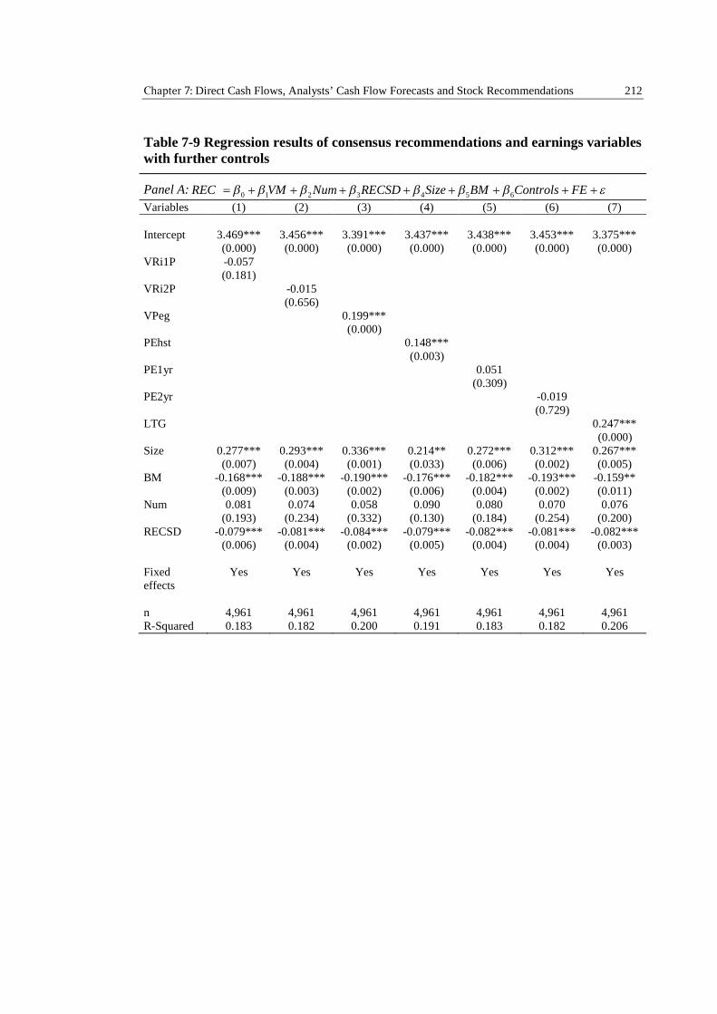
Chapter 7: Direct Cash Flows, Analysts’ Cash Flow Forecasts and Stock Recommendations 212
Table 7-9 Regression results of consensus recommendations and earnings variableswith further controls
Panel A: 0 1 2 3 4 5 6REC VM Num RECSD Size BM Controls FE
Variables (1) (2) (3) (4) (5) (6) (7)
Intercept 3.469*** 3.456*** 3.391*** 3.437*** 3.438*** 3.453*** 3.375***(0.000) (0.000) (0.000) (0.000) (0.000) (0.000) (0.000)
VRi1P -0.057(0.181)
VRi2P -0.015(0.656)
VPeg 0.199***(0.000)
PEhst 0.148***(0.003)
PE1yr 0.051(0.309)
PE2yr -0.019(0.729)
LTG 0.247***(0.000)
Size 0.277*** 0.293*** 0.336*** 0.214** 0.272*** 0.312*** 0.267***(0.007) (0.004) (0.001) (0.033) (0.006) (0.002) (0.005)
BM -0.168*** -0.188*** -0.190*** -0.176*** -0.182*** -0.193*** -0.159**(0.009) (0.003) (0.002) (0.006) (0.004) (0.002) (0.011)
Num 0.081 0.074 0.058 0.090 0.080 0.070 0.076(0.193) (0.234) (0.332) (0.130) (0.184) (0.254) (0.200)
RECSD -0.079*** -0.081*** -0.084*** -0.079*** -0.082*** -0.081*** -0.082***(0.006) (0.004) (0.002) (0.005) (0.004) (0.004) (0.003)
Fixedeffects
Yes Yes Yes Yes Yes Yes Yes
n 4,961 4,961 4,961 4,961 4,961 4,961 4,961R-Squared 0.183 0.182 0.200 0.191 0.183 0.182 0.206
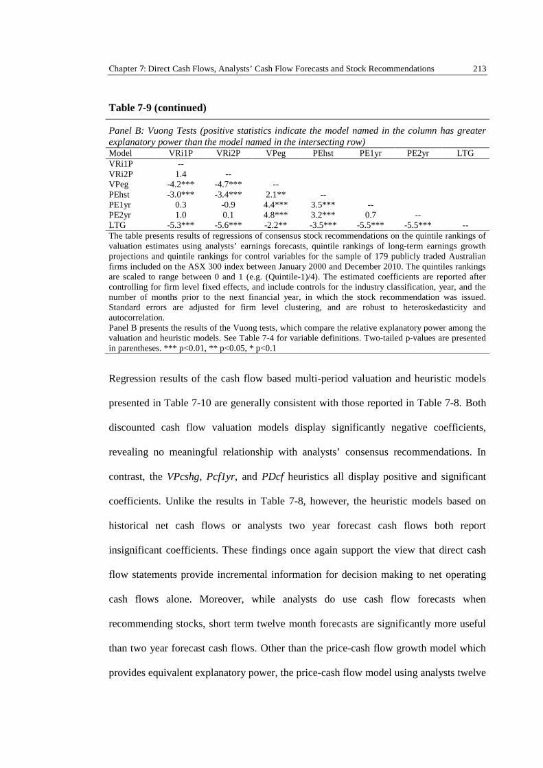
Chapter 7: Direct Cash Flows, Analysts’ Cash Flow Forecasts and Stock Recommendations 213
Table 7-9 (continued)
Panel B: Vuong Tests (positive statistics indicate the model named in the column has greaterexplanatory power than the model named in the intersecting row)Model VRi1P VRi2P VPeg PEhst PE1yr PE2yr LTGVRi1P --VRi2P 1.4 --VPeg -4.2*** -4.7*** --PEhst -3.0*** -3.4*** 2.1** --PE1yr 0.3 -0.9 4.4*** 3.5*** --PE2yr 1.0 0.1 4.8*** 3.2*** 0.7 --LTG -5.3*** -5.6*** -2.2** -3.5*** -5.5*** -5.5*** --The table presents results of regressions of consensus stock recommendations on the quintile rankings ofvaluation estimates using analysts’ earnings forecasts, quintile rankings of long-term earnings growthprojections and quintile rankings for control variables for the sample of 179 publicly traded Australianfirms included on the ASX 300 index between January 2000 and December 2010. The quintiles rankingsare scaled to range between 0 and 1 (e.g. (Quintile-1)/4). The estimated coefficients are reported aftercontrolling for firm level fixed effects, and include controls for the industry classification, year, and thenumber of months prior to the next financial year, in which the stock recommendation was issued.Standard errors are adjusted for firm level clustering, and are robust to heteroskedasticity andautocorrelation.Panel B presents the results of the Vuong tests, which compare the relative explanatory power among thevaluation and heuristic models. See Table 7-4 for variable definitions. Two-tailed p-values are presentedin parentheses. *** p<0.01, ** p<0.05, * p<0.1
Regression results of the cash flow based multi-period valuation and heuristic models
presented in Table 7-10 are generally consistent with those reported in Table 7-8. Both
discounted cash flow valuation models display significantly negative coefficients,
revealing no meaningful relationship with analysts’ consensus recommendations. In
contrast, the VPcshg, Pcf1yr, and PDcf heuristics all display positive and significant
coefficients. Unlike the results in Table 7-8, however, the heuristic models based on
historical net cash flows or analysts two year forecast cash flows both report
insignificant coefficients. These findings once again support the view that direct cash
flow statements provide incremental information for decision making to net operating
cash flows alone. Moreover, while analysts do use cash flow forecasts when
recommending stocks, short term twelve month forecasts are significantly more useful
than two year forecast cash flows. Other than the price-cash flow growth model which
provides equivalent explanatory power, the price-cash flow model using analysts twelve
Chapter 7: Direct Cash Flows, Analysts’ Cash Flow Forecasts and Stock Recommendations 214
month forecast is by far the superior cash flow based heuristic used by analysts when
recommending stocks. This contrasts with the use of earnings based heuristics in Table
7-9, which reveal historical price-earnings models provide analysts with more useful
information than price-earnings models based on analysts forecast earnings. Taken
altogether the findings in both Table 7-9 and Table 7-10, with additional controls,
provide consistent evidence with the findings from the less restrictive models, and
provide strong support for H1a, H1b, and H2.
7.5.3 Analysis of Changes in Recommendations on Changes in Valuation
Metrics
In addition to the models use above, following Bradshaw (2004), H1 and H2 are further
examined by regressing the changes in analysts’ consensus stock recommendations on
the quintile rankings of the changes in the valuation and heuristic measures calculated
using Equations (7.1) to (7.9):
0 1 2REC VM Controls FE (7.12)
Where REC is the change in analysts’ average consensus recommendation, VM is
the change in the multi-period valuation or heuristic measure, FE are firm level fixed
effects, and Controls include controls for the industry classification, year, and the
number of months prior to the next financial year, in which the stock recommendation
was issued. Due to missing lagged measures for REC and VM, which are required to
calculate the dependent and independent variables used in Equation (7.12), 2,072 firm
month observations are removed from the sample, leaving 2,889 firm month
observations without missing data requirements.
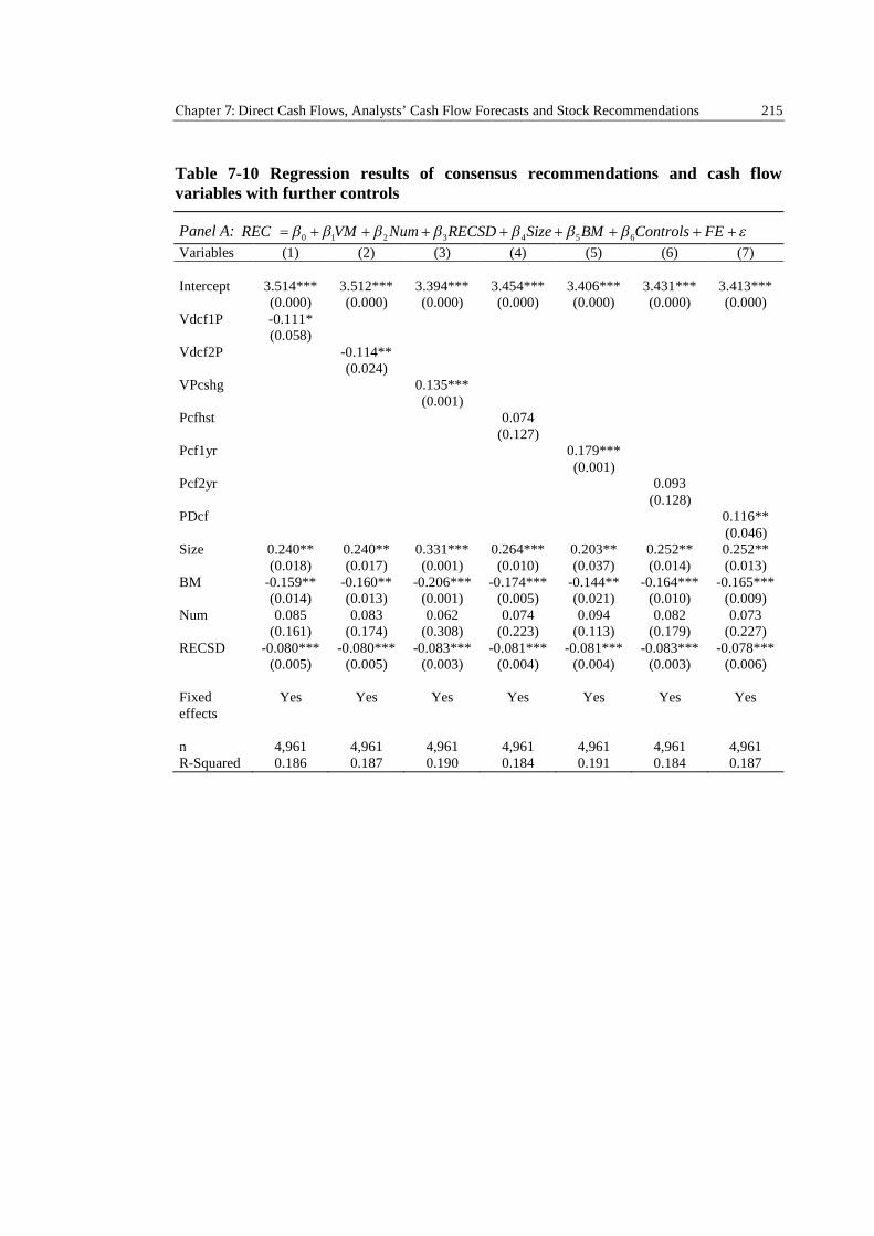
Chapter 7: Direct Cash Flows, Analysts’ Cash Flow Forecasts and Stock Recommendations 215
Table 7-10 Regression results of consensus recommendations and cash flowvariables with further controls
Panel A: 0 1 2 3 4 5 6REC VM Num RECSD Size BM Controls FE
Variables (1) (2) (3) (4) (5) (6) (7)
Intercept 3.514*** 3.512*** 3.394*** 3.454*** 3.406*** 3.431*** 3.413***(0.000) (0.000) (0.000) (0.000) (0.000) (0.000) (0.000)
Vdcf1P -0.111*(0.058)
Vdcf2P -0.114**(0.024)
VPcshg 0.135***(0.001)
Pcfhst 0.074(0.127)
Pcf1yr 0.179***(0.001)
Pcf2yr 0.093(0.128)
PDcf 0.116**(0.046)
Size 0.240** 0.240** 0.331*** 0.264*** 0.203** 0.252** 0.252**(0.018) (0.017) (0.001) (0.010) (0.037) (0.014) (0.013)
BM -0.159** -0.160** -0.206*** -0.174*** -0.144** -0.164*** -0.165***(0.014) (0.013) (0.001) (0.005) (0.021) (0.010) (0.009)
Num 0.085 0.083 0.062 0.074 0.094 0.082 0.073(0.161) (0.174) (0.308) (0.223) (0.113) (0.179) (0.227)
RECSD -0.080*** -0.080*** -0.083*** -0.081*** -0.081*** -0.083*** -0.078***(0.005) (0.005) (0.003) (0.004) (0.004) (0.003) (0.006)
Fixedeffects
Yes Yes Yes Yes Yes Yes Yes
n 4,961 4,961 4,961 4,961 4,961 4,961 4,961R-Squared 0.186 0.187 0.190 0.184 0.191 0.184 0.187
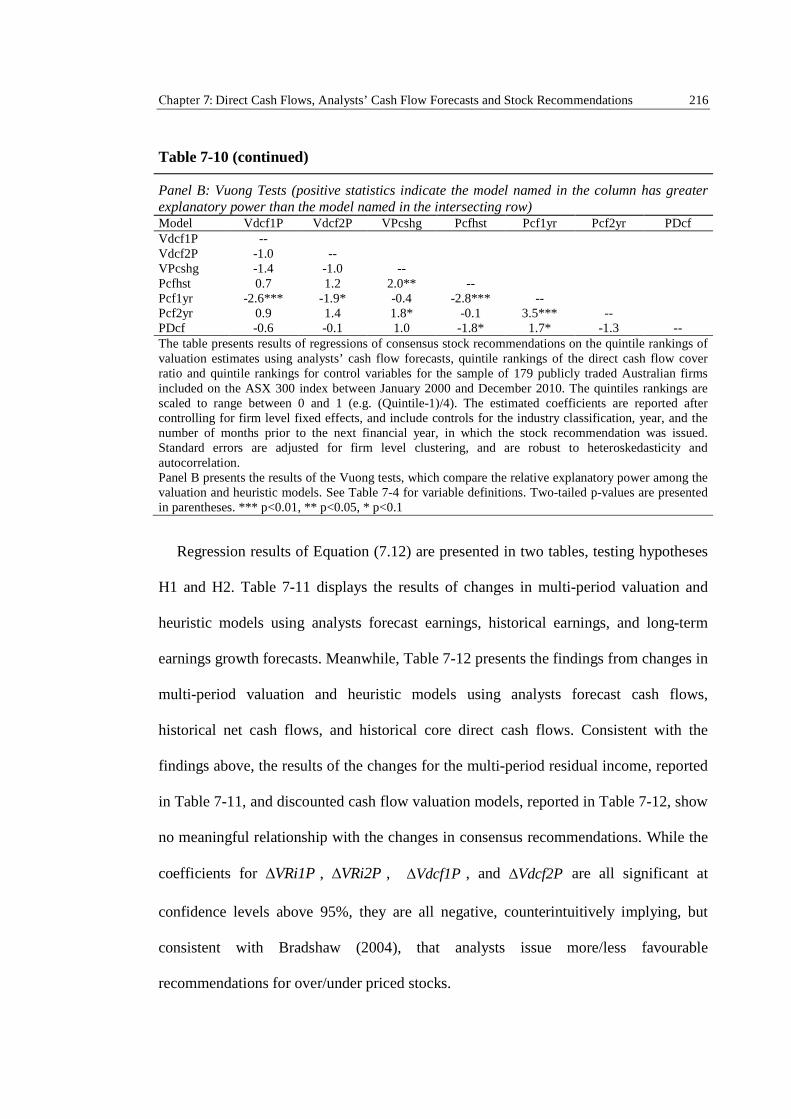
Chapter 7: Direct Cash Flows, Analysts’ Cash Flow Forecasts and Stock Recommendations 216
Table 7-10 (continued)
Panel B: Vuong Tests (positive statistics indicate the model named in the column has greaterexplanatory power than the model named in the intersecting row)Model Vdcf1P Vdcf2P VPcshg Pcfhst Pcf1yr Pcf2yr PDcfVdcf1P --Vdcf2P -1.0 --VPcshg -1.4 -1.0 --Pcfhst 0.7 1.2 2.0** --Pcf1yr -2.6*** -1.9* -0.4 -2.8*** --Pcf2yr 0.9 1.4 1.8* -0.1 3.5*** --PDcf -0.6 -0.1 1.0 -1.8* 1.7* -1.3 --The table presents results of regressions of consensus stock recommendations on the quintile rankings ofvaluation estimates using analysts’ cash flow forecasts, quintile rankings of the direct cash flow coverratio and quintile rankings for control variables for the sample of 179 publicly traded Australian firmsincluded on the ASX 300 index between January 2000 and December 2010. The quintiles rankings arescaled to range between 0 and 1 (e.g. (Quintile-1)/4). The estimated coefficients are reported aftercontrolling for firm level fixed effects, and include controls for the industry classification, year, and thenumber of months prior to the next financial year, in which the stock recommendation was issued.Standard errors are adjusted for firm level clustering, and are robust to heteroskedasticity andautocorrelation.Panel B presents the results of the Vuong tests, which compare the relative explanatory power among thevaluation and heuristic models. See Table 7-4 for variable definitions. Two-tailed p-values are presentedin parentheses. *** p<0.01, ** p<0.05, * p<0.1
Regression results of Equation (7.12) are presented in two tables, testing hypotheses
H1 and H2. Table 7-11 displays the results of changes in multi-period valuation and
heuristic models using analysts forecast earnings, historical earnings, and long-term
earnings growth forecasts. Meanwhile, Table 7-12 presents the findings from changes in
multi-period valuation and heuristic models using analysts forecast cash flows,
historical net cash flows, and historical core direct cash flows. Consistent with the
findings above, the results of the changes for the multi-period residual income, reported
in Table 7-11, and discounted cash flow valuation models, reported in Table 7-12, show
no meaningful relationship with the changes in consensus recommendations. While the
coefficients for VRi1P , VRi2P , Vdcf1P , and Vdcf2P are all significant at
confidence levels above 95%, they are all negative, counterintuitively implying, but
consistent with Bradshaw (2004), that analysts issue more/less favourable
recommendations for over/under priced stocks.
Chapter 7: Direct Cash Flows, Analysts’ Cash Flow Forecasts and Stock Recommendations 217
In line with H1a, the coefficients of the changes in earnings based heuristic models
reported in Table 7-11 are all positive. However, while PE2yr is the only
insignificant model, PEhst and LTG are the only models which are significant at
confidence levels above 95%. Increasing PEhst from the lowest to the highest quintile
ranking, results in an overall 0.062 change in analysts’ consensus recommendation,
higher than the 0.04 change from the LTG coefficient. Analysts clearly increase their
recommendation levels in response to positive changes in historical earnings and long-
term earnings growth forecasts. Vuong tests show that, PEhst dominates all other
models, with the exception of LTG where there is no significant difference, further
emphasising the importance analysts place on these valuation heuristics when
recommending stocks.
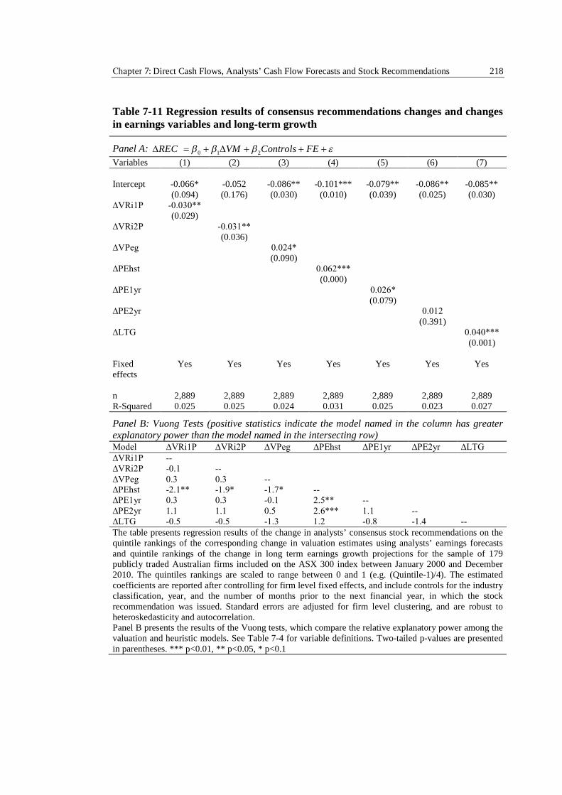
Chapter 7: Direct Cash Flows, Analysts’ Cash Flow Forecasts and Stock Recommendations 218
Table 7-11 Regression results of consensus recommendations changes and changesin earnings variables and long-term growth
Panel A: 0 1 2REC VM Controls FE
Variables (1) (2) (3) (4) (5) (6) (7)
Intercept -0.066* -0.052 -0.086** -0.101*** -0.079** -0.086** -0.085**(0.094) (0.176) (0.030) (0.010) (0.039) (0.025) (0.030)
∆VRi1P -0.030** (0.029)
∆VRi2P -0.031** (0.036)
∆VPeg 0.024* (0.090)
∆PEhst 0.062*** (0.000)
∆PE1yr 0.026* (0.079)
∆PE2yr 0.012 (0.391)
∆LTG 0.040*** (0.001)
Fixedeffects
Yes Yes Yes Yes Yes Yes Yes
n 2,889 2,889 2,889 2,889 2,889 2,889 2,889R-Squared 0.025 0.025 0.024 0.031 0.025 0.023 0.027
Panel B: Vuong Tests (positive statistics indicate the model named in the column has greaterexplanatory power than the model named in the intersecting row)Model ∆VRi1P ∆VRi2P ∆VPeg ∆PEhst ∆PE1yr ∆PE2yr ∆LTG ∆VRi1P -- ∆VRi2P -0.1 -- ∆VPeg 0.3 0.3 -- ∆PEhst -2.1** -1.9* -1.7* -- ∆PE1yr 0.3 0.3 -0.1 2.5** -- ∆PE2yr 1.1 1.1 0.5 2.6*** 1.1 -- ∆LTG -0.5 -0.5 -1.3 1.2 -0.8 -1.4 -- The table presents regression results of the change in analysts’ consensus stock recommendations on thequintile rankings of the corresponding change in valuation estimates using analysts’ earnings forecastsand quintile rankings of the change in long term earnings growth projections for the sample of 179publicly traded Australian firms included on the ASX 300 index between January 2000 and December2010. The quintiles rankings are scaled to range between 0 and 1 (e.g. (Quintile-1)/4). The estimatedcoefficients are reported after controlling for firm level fixed effects, and include controls for the industryclassification, year, and the number of months prior to the next financial year, in which the stockrecommendation was issued. Standard errors are adjusted for firm level clustering, and are robust toheteroskedasticity and autocorrelation.Panel B presents the results of the Vuong tests, which compare the relative explanatory power among thevaluation and heuristic models. See Table 7-4 for variable definitions. Two-tailed p-values are presentedin parentheses. *** p<0.01, ** p<0.05, * p<0.1
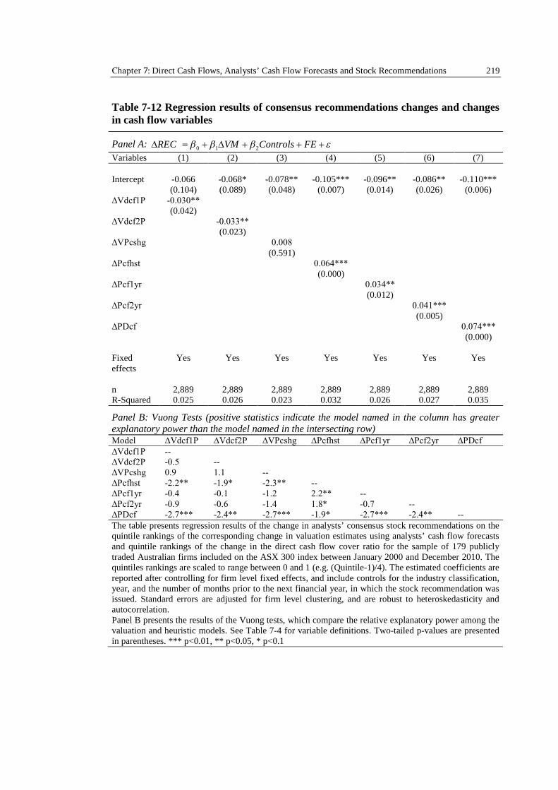
Chapter 7: Direct Cash Flows, Analysts’ Cash Flow Forecasts and Stock Recommendations 219
Table 7-12 Regression results of consensus recommendations changes and changesin cash flow variables
Panel A: 0 1 2REC VM Controls FE
Variables (1) (2) (3) (4) (5) (6) (7)
Intercept -0.066 -0.068* -0.078** -0.105*** -0.096** -0.086** -0.110***(0.104) (0.089) (0.048) (0.007) (0.014) (0.026) (0.006)
∆Vdcf1P -0.030** (0.042)
∆Vdcf2P -0.033** (0.023)
∆VPcshg 0.008 (0.591)
∆Pcfhst 0.064*** (0.000)
∆Pcf1yr 0.034** (0.012)
∆Pcf2yr 0.041*** (0.005)
∆PDcf 0.074*** (0.000)
Fixedeffects
Yes Yes Yes Yes Yes Yes Yes
n 2,889 2,889 2,889 2,889 2,889 2,889 2,889R-Squared 0.025 0.026 0.023 0.032 0.026 0.027 0.035
Panel B: Vuong Tests (positive statistics indicate the model named in the column has greaterexplanatory power than the model named in the intersecting row)Model ∆Vdcf1P ∆Vdcf2P ∆VPcshg ∆Pcfhst ∆Pcf1yr ∆Pcf2yr ∆PDcf ∆Vdcf1P -- ∆Vdcf2P -0.5 -- ∆VPcshg 0.9 1.1 -- ∆Pcfhst -2.2** -1.9* -2.3** -- ∆Pcf1yr -0.4 -0.1 -1.2 2.2** -- ∆Pcf2yr -0.9 -0.6 -1.4 1.8* -0.7 -- ∆PDcf -2.7*** -2.4** -2.7*** -1.9* -2.7*** -2.4** -- The table presents regression results of the change in analysts’ consensus stock recommendations on thequintile rankings of the corresponding change in valuation estimates using analysts’ cash flow forecastsand quintile rankings of the change in the direct cash flow cover ratio for the sample of 179 publiclytraded Australian firms included on the ASX 300 index between January 2000 and December 2010. Thequintiles rankings are scaled to range between 0 and 1 (e.g. (Quintile-1)/4). The estimated coefficients arereported after controlling for firm level fixed effects, and include controls for the industry classification,year, and the number of months prior to the next financial year, in which the stock recommendation wasissued. Standard errors are adjusted for firm level clustering, and are robust to heteroskedasticity andautocorrelation.Panel B presents the results of the Vuong tests, which compare the relative explanatory power among thevaluation and heuristic models. See Table 7-4 for variable definitions. Two-tailed p-values are presentedin parentheses. *** p<0.01, ** p<0.05, * p<0.1
Chapter 7: Direct Cash Flows, Analysts’ Cash Flow Forecasts and Stock Recommendations 220
Results from the changes in cash flow based multi-period valuation and heuristic
models reported by Table 7-12 provide further support for the findings already
documented in the previous tests. With the exception of VPcshg , all the cash flow
based heuristics coefficients are positive and significant at confidence levels above
95%. Moreover, while changes in heuristics based on analysts’ cash flow forecasts,
Pcf1yr and Pcf2yr , are positively related to changes in recommendations,
supporting H1a, heuristics based on the changes in historical cash flows explain more of
the changes in analysts’ recommendations. However, in contrast to the results using
recommendation and valuation metric levels, but consistent with H1b, Vuong tests
show that changes in analysts’ consensus recommendations are best explained by
changes in the direct cash flow heuristic, PDcf . Changes in historical net operating
cash flows, Pcfhst , are the second best cash flow heuristic. These findings provide
further strong evidence for the usefulness of direct cash flow information over and
above net operating cash flows alone.
7.5.4 Analysis of Future Excess Returns and Valuation Models
The final analyses, addressing H3, investigates the profitability of identifying mispriced
stocks by following analysts’ recommendations or heuristic valuations compared to
buy-and-hold investors exploiting analysts’ earnings and cash flow forecasts in multi-
period valuation models. Market and size adjusted future returns are used as the
dependent variables to capture future buy-and-hold excess returns. Although prior
studies generally use size-adjusted returns, market adjusted returns are also used in this
chapter since the sample is comprised of only those firms listed on the ASX300 index.
Future buy-and-hold one-year market-adjusted returns (CAR) are calculated as follows:
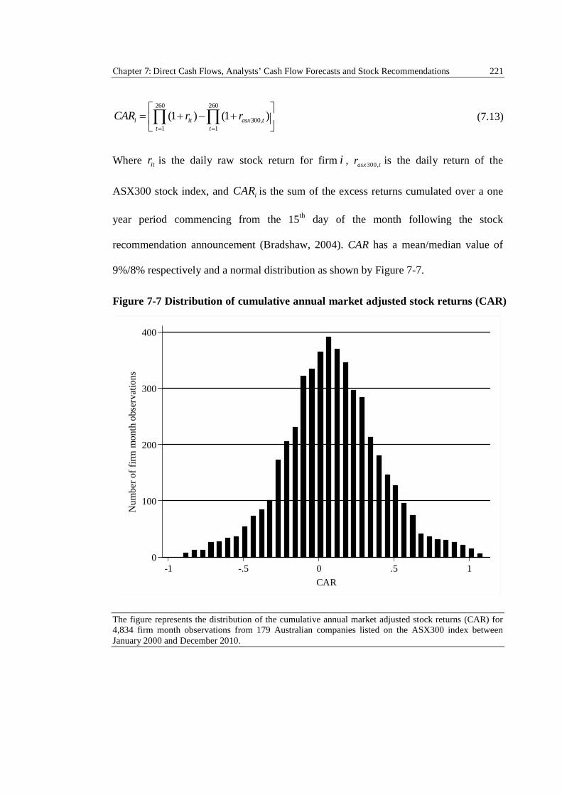
Chapter 7: Direct Cash Flows, Analysts’ Cash Flow Forecasts and Stock Recommendations 221
260 260
300,1 1
(1 ) (1 )i it asx tt t
CAR r r
(7.13)
Where itr is the daily raw stock return for firm i , 300,asx tr is the daily return of the
ASX300 stock index, and iCAR is the sum of the excess returns cumulated over a one
year period commencing from the 15th day of the month following the stock
recommendation announcement (Bradshaw, 2004). CAR has a mean/median value of
9%/8% respectively and a normal distribution as shown by Figure 7-7.
Figure 7-7 Distribution of cumulative annual market adjusted stock returns (CAR)
The figure represents the distribution of the cumulative annual market adjusted stock returns (CAR) for4,834 firm month observations from 179 Australian companies listed on the ASX300 index betweenJanuary 2000 and December 2010.
0
100
200
300
400
Num
ber
offi
rmm
onth
obs
erva
tion
s
-1 -.5 0 .5 1
CAR
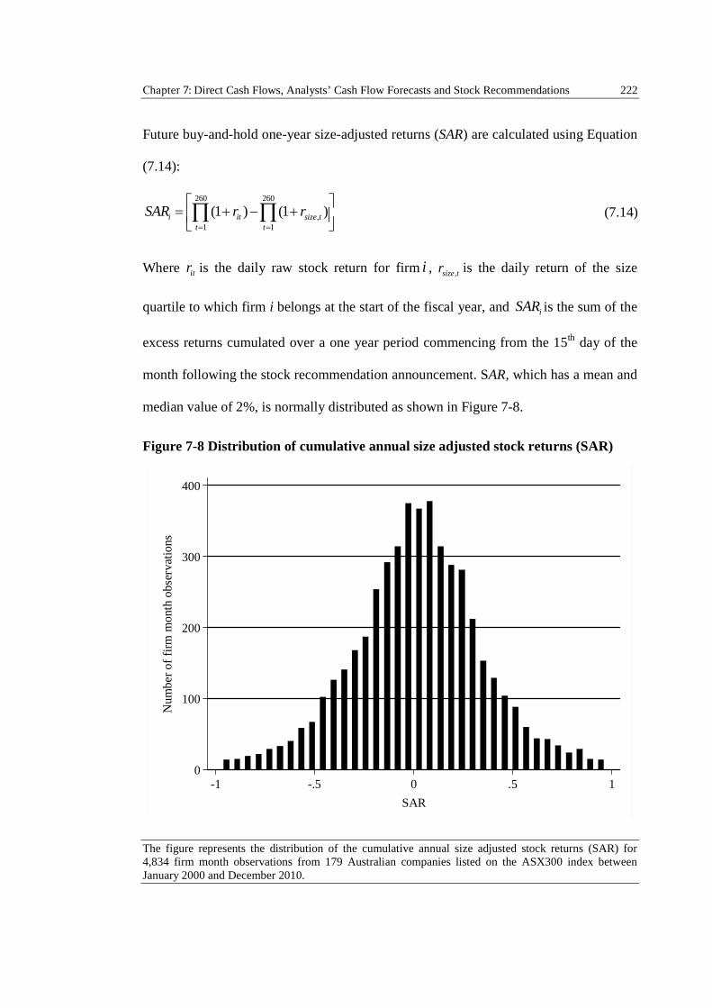
Chapter 7: Direct Cash Flows, Analysts’ Cash Flow Forecasts and Stock Recommendations 222
Future buy-and-hold one-year size-adjusted returns (SAR) are calculated using Equation
(7.14):
260 260
,1 1
(1 ) (1 )i it size tt t
SAR r r
(7.14)
Where itr is the daily raw stock return for firm i , ,size tr is the daily return of the size
quartile to which firm i belongs at the start of the fiscal year, and iSAR is the sum of the
excess returns cumulated over a one year period commencing from the 15th day of the
month following the stock recommendation announcement. SAR, which has a mean and
median value of 2%, is normally distributed as shown in Figure 7-8.
Figure 7-8 Distribution of cumulative annual size adjusted stock returns (SAR)
The figure represents the distribution of the cumulative annual size adjusted stock returns (SAR) for4,834 firm month observations from 179 Australian companies listed on the ASX300 index betweenJanuary 2000 and December 2010.
0
100
200
300
400
Nu
mb
ero
ffi
rmm
ont
ho
bse
rvat
ion
s
-1 -.5 0 .5 1
SAR
Chapter 7: Direct Cash Flows, Analysts’ Cash Flow Forecasts and Stock Recommendations 223
Employing a similar model to Bradshaw (2004), the excess returns calculated in
Equations (7.13) and (7.14) are now each used as the dependent variable in the
following regression:
0 1 2Ret VM Controls FE (7.15)
Where Ret is the buy-and-hold one-year market-adjusted ( iCAR ) or size-adjusted
( iSAR ) excess returns calculated using either Equation (7.13) or Equation (7.14). VM is
the multi-period valuation or heuristic model calculated using Equations (7.1) to (7.9),
FE are firm level fixed effects, and Controls include controls for the industry
classification, year, and the number of months prior to the next financial year, in which
the stock recommendation was issued. Regression results of Equation (7.15) are
presented in four tables. Results of the future excess market-adjusted returns are shown
in Table 7-13 and Table 7-15, while the results of future excess size-adjusted returns are
reported in Table 7-14 and Table 7-16. Results of the earnings based multi-period
valuation and heuristic models, and the long-term earnings growth forecasts are
presented in Table 7-13 and Table 7-14, while Table 7-15 and Table 7-16 present the
findings from the cash flow valuation and heuristic models. Vuong tests are used to
compare the explanatory power between the different models and are reported in Panel
B of each table. Finally, Vuong tests are used to compare the explanatory power
between the earnings and cash flow valuation and heuristic models, and are presented in
Table 7-17.

Chapter 7: Direct Cash Flows, Analysts’ Cash Flow Forecasts and Stock Recommendations 224
Table 7-13 Regression results of one-year-ahead market adjusted returns onconsensus recommendations, earnings variables, and long term growth
Panel A: 0 1 2CAR VM Controls FE
Variables (1) (2) (3) (4) (5) (6) (7) (8)
Intercept 0.049 -0.032 0.002 0.058 0.100*** 0.107*** 0.112*** 0.091**(0.197) (0.390) (0.947) (0.118) (0.006) (0.004) (0.003) (0.012)
REC -0.036(0.227)
VRi1P 0.137***(0.000)
VRi2P 0.067**(0.013)
VPeg -0.060*(0.054)
PEhst -0.197***(0.000)
PE1yr -0.185***(0.000)
PE2yr -0.194***(0.000)
LTG -0.154***(0.000)
Fixedeffects
Yes Yes Yes Yes Yes Yes Yes Yes
n 4,834 4,834 4,834 4,834 4,834 4,834 4,834 4,834R-Squared 0.117 0.129 0.120 0.118 0.144 0.137 0.137 0.132
Panel B: Vuong Tests (positive statistics indicate the model named in the column has greaterexplanatory power than the model named in the intersecting row)Model REC VRi1P VRi2P VPeg PEhst PE1yr PE2yr LTGREC --VRi1P -3.6*** --VRi2P -1.5 4.0*** --VPeg -1.1 2.6*** 0.5 --PEhst -5.6*** -3.2*** -5.0*** -4.9*** --PE1yr -5.0*** -2.2** -4.6*** -4.2*** 1.6 --PE2yr -5.1*** -2.3** -4.7*** -4.1*** 1.5 -0.1 --LTG -4.3*** -0.8 -3.2*** -4.8*** 2.3** 1.1 1.1 --The table presents regression results of the one-year-ahead market adjusted returns on the quintilerankings of analysts’ consensus stock recommendations and valuation estimates using analysts’ earningsforecasts, and quintile rankings of long term earnings growth projections for the sample of 179 publiclytraded Australian firms included on the ASX 300 index between January 2000 and December 2010. Thequintiles rankings are scaled to range between 0 and 1 (e.g. (Quintile-1)/4). The estimated coefficients arereported after controlling for firm level fixed effects, and include controls for the industry classification,year, and the number of months prior to the next financial year, in which the stock recommendation wasissued. Standard errors are adjusted for firm level clustering, and are robust to heteroskedasticity andautocorrelation.Panel B presents the results of the Vuong tests, which compare the relative explanatory power among thevaluation and heuristic models. See Table 7-4 for variable definitions. Two-tailed p-values are presentedin parentheses. *** p<0.01, ** p<0.05, * p<0.1
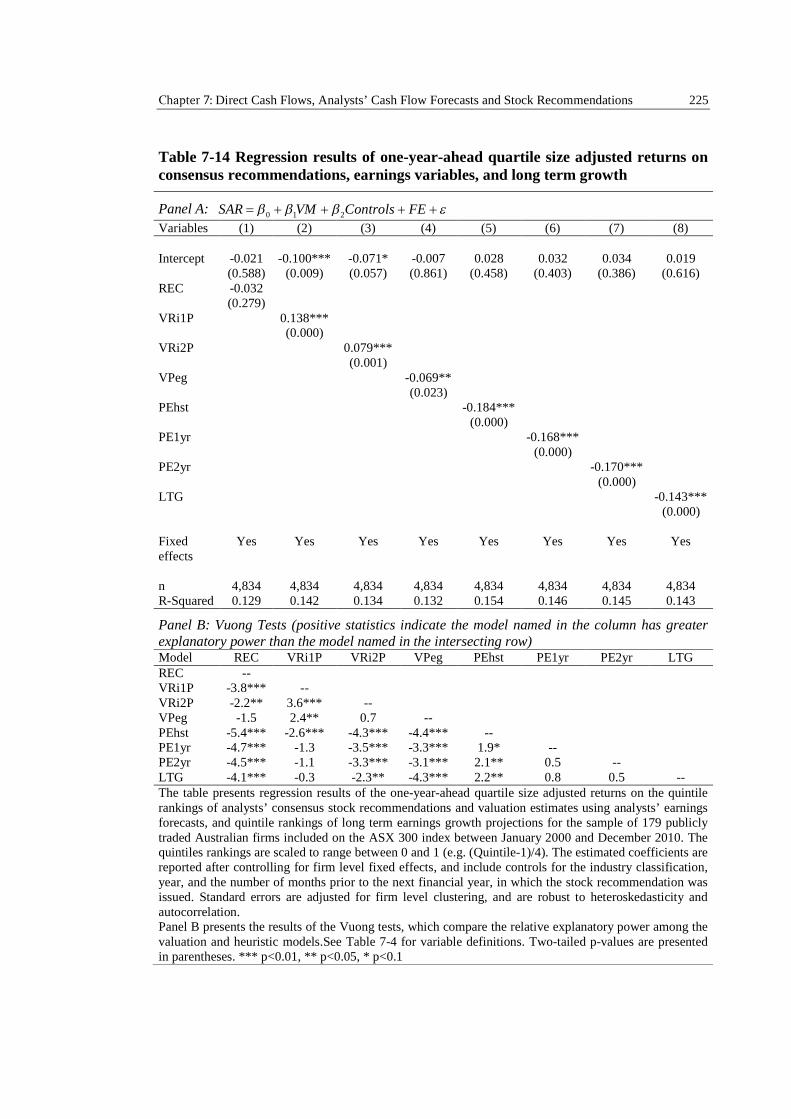
Chapter 7: Direct Cash Flows, Analysts’ Cash Flow Forecasts and Stock Recommendations 225
Table 7-14 Regression results of one-year-ahead quartile size adjusted returns onconsensus recommendations, earnings variables, and long term growth
Panel A: 0 1 2SAR VM Controls FE
Variables (1) (2) (3) (4) (5) (6) (7) (8)
Intercept -0.021 -0.100*** -0.071* -0.007 0.028 0.032 0.034 0.019(0.588) (0.009) (0.057) (0.861) (0.458) (0.403) (0.386) (0.616)
REC -0.032(0.279)
VRi1P 0.138***(0.000)
VRi2P 0.079***(0.001)
VPeg -0.069**(0.023)
PEhst -0.184***(0.000)
PE1yr -0.168***(0.000)
PE2yr -0.170***(0.000)
LTG -0.143***(0.000)
Fixedeffects
Yes Yes Yes Yes Yes Yes Yes Yes
n 4,834 4,834 4,834 4,834 4,834 4,834 4,834 4,834R-Squared 0.129 0.142 0.134 0.132 0.154 0.146 0.145 0.143
Panel B: Vuong Tests (positive statistics indicate the model named in the column has greaterexplanatory power than the model named in the intersecting row)Model REC VRi1P VRi2P VPeg PEhst PE1yr PE2yr LTGREC --VRi1P -3.8*** --VRi2P -2.2** 3.6*** --VPeg -1.5 2.4** 0.7 --PEhst -5.4*** -2.6*** -4.3*** -4.4*** --PE1yr -4.7*** -1.3 -3.5*** -3.3*** 1.9* --PE2yr -4.5*** -1.1 -3.3*** -3.1*** 2.1** 0.5 --LTG -4.1*** -0.3 -2.3** -4.3*** 2.2** 0.8 0.5 --The table presents regression results of the one-year-ahead quartile size adjusted returns on the quintilerankings of analysts’ consensus stock recommendations and valuation estimates using analysts’ earningsforecasts, and quintile rankings of long term earnings growth projections for the sample of 179 publiclytraded Australian firms included on the ASX 300 index between January 2000 and December 2010. Thequintiles rankings are scaled to range between 0 and 1 (e.g. (Quintile-1)/4). The estimated coefficients arereported after controlling for firm level fixed effects, and include controls for the industry classification,year, and the number of months prior to the next financial year, in which the stock recommendation wasissued. Standard errors are adjusted for firm level clustering, and are robust to heteroskedasticity andautocorrelation.Panel B presents the results of the Vuong tests, which compare the relative explanatory power among thevaluation and heuristic models.See Table 7-4 for variable definitions. Two-tailed p-values are presentedin parentheses. *** p<0.01, ** p<0.05, * p<0.1
Chapter 7: Direct Cash Flows, Analysts’ Cash Flow Forecasts and Stock Recommendations 226
Results from Table 7-13 and Table 7-14 show insignificant coefficients for REC,
corroborating findings of earlier studies that show buy-and-hold investors fail to earn
positive excess annual stock returns by following analysts’ consensus stock
recommendations. However, coefficients on VPeg, PEhst, PE1yr, PE2yr, and LTG are
all negative and, with the exception of VPeg in Table 7-13, significant at confidence
levels above 95%. While analysts find earnings based valuation heuristics useful when
issuing their stock recommendations, buy-and-hold investors fail to earn significant
positive excess annual returns by using earnings based valuation heuristics and long-
term earnings growth predictions to identify mispriced stocks. Conversely, coefficients
for VRi1P and VRri2P are both positive and significant at confidence levels above 95%.
Consistent with prior studies (e.g., Bradshaw, 2004; Barniv et al., 2009; Barniv et al.,
2010), buy-and-hold investors do earn significant positive excess annual returns by
identifying mispriced securities using analysts’ earnings forecasts in residual income
models.
Interpreting the Vuong tests reported in Panel B of Table 7-13 and Table 7-14 should
be done with caution. For example, while the test statistics imply that PEhst model has
the greatest explanatory power for future excess returns, the coefficients for PEhst are
significantly negative at confidence levels above 95%. Effectively this shows that buy-
and-hold investors using PEhst to identify mispriced securities earn annual returns that
are significantly below the average returns of the market and size portfolio.
Accordingly, while Vuong test statistics are shown for all models, the interpretation of
these statistics is limited to those models with positive coefficients, showing that VRi1P
is significantly more profitable for buy-and-hold investors than VRri2P.
Chapter 7: Direct Cash Flows, Analysts’ Cash Flow Forecasts and Stock Recommendations 227
Findings from the cash flow valuation and heuristic models are reported in Table
7-15 and Table 7-16 and show significantly positive coefficients for Vdcf1P and Vdcf2P
at confidence levels above 95%. Conversely, with the exception of VPcshg, coefficients
for all the cash flow based heuristic measures are negative and highly significant. These
findings affirm H3 and are consistent with the earnings models reported in Table 7-13
and Table 7-14. Buy-and-hold investors can earn future excess annual returns by
identifying mispriced securities using analysts’ earnings or cash flow forecasts in multi-
period models. However, relying on simple heuristics to identify mispriced stocks can
lead buy-and-hold investors to earn returns that are significantly below the average
market and size portfolio returns. Once again restricting the analysis of the Vuong tests
reported in Panel B of Table 7-15 and Table 7-16 to those models with positive
coefficients, the results show that identifying mispriced securities using Vdcf1P is
significantly more profitable for buy-and-hold investors than Vdcf2P.

Chapter 7: Direct Cash Flows, Analysts’ Cash Flow Forecasts and Stock Recommendations 228
Table 7-15 Regression results of one-year-ahead market adjusted returns on cashflow variables
Panel A: 0 1 2CAR VM Controls FE
Variables (1) (2) (3) (4) (5) (6) (7)
Intercept -0.091** -0.059 0.054 0.096** 0.120*** 0.103*** 0.119***(0.032) (0.138) (0.152) (0.013) (0.003) (0.005) (0.002)
Vdcf1P 0.215***(0.000)
Vdcf2P 0.164***(0.000)
VPcshg -0.047(0.161)
Pcfhst -0.192***(0.000)
Pcf1yr -0.234***(0.000)
Pcf2yr -0.228***(0.000)
PDcf -0.243***(0.000)
Fixedeffects
Yes Yes Yes Yes Yes Yes Yes
n 4,834 4,834 4,834 4,834 4,834 4,834 4,834R-Squared 0.142 0.134 0.117 0.143 0.147 0.144 0.154
Panel B: Vuong Tests (positive statistics indicate the model named in the column has greaterexplanatory power than the model named in the intersecting row)Model Vdcf1P Vdcf2P VPcshg Pcfhst Pcf1yr Pcf2yr PDcfVdcf1P --Vdcf2P 3.3*** --VPcshg 4.6*** 3.8*** --Pcfhst -0.2 -1.8* -5.0*** --Pcf1yr -1.3 -3.0*** -5.5*** -0.9 --Pcf2yr -0.5 -2.4** -5.0*** -0.1 1.2 --PDcf -2.1** -3.6*** -6.1*** -2.6** -1.2 -1.9* --The table presents regression results of the one-year-ahead market adjusted returns on the quintilerankings of valuation estimates using analysts’ cash flow forecasts and quintile rankings of the direct cashflow cover ratio for the sample of 179 publicly traded Australian firms included on the ASX 300 indexbetween January 2000 and December 2010. The quintiles rankings are scaled to range between 0 and 1(e.g. (Quintile-1)/4). The estimated coefficients are reported after controlling for firm level fixed effects,and include controls for the industry classification, year, and the number of months prior to the nextfinancial year, in which the stock recommendation was issued. Standard errors are adjusted for firm levelclustering, and are robust to heteroskedasticity and autocorrelation.Panel B presents the results of the Vuong tests, which compare the relative explanatory power among thevaluation and heuristic models.See Table 7-4 for variable definitions. Two-tailed p-values are presented in parentheses. *** p<0.01, **p<0.05, * p<0.1
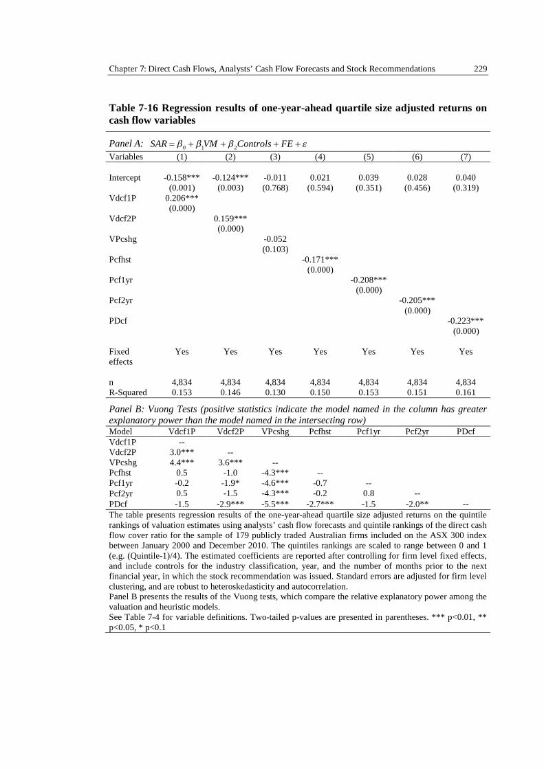
Chapter 7: Direct Cash Flows, Analysts’ Cash Flow Forecasts and Stock Recommendations 229
Table 7-16 Regression results of one-year-ahead quartile size adjusted returns oncash flow variables
Panel A: 0 1 2SAR VM Controls FE
Variables (1) (2) (3) (4) (5) (6) (7)
Intercept -0.158*** -0.124*** -0.011 0.021 0.039 0.028 0.040(0.001) (0.003) (0.768) (0.594) (0.351) (0.456) (0.319)
Vdcf1P 0.206***(0.000)
Vdcf2P 0.159***(0.000)
VPcshg -0.052(0.103)
Pcfhst -0.171***(0.000)
Pcf1yr -0.208***(0.000)
Pcf2yr -0.205***(0.000)
PDcf -0.223***(0.000)
Fixedeffects
Yes Yes Yes Yes Yes Yes Yes
n 4,834 4,834 4,834 4,834 4,834 4,834 4,834R-Squared 0.153 0.146 0.130 0.150 0.153 0.151 0.161
Panel B: Vuong Tests (positive statistics indicate the model named in the column has greaterexplanatory power than the model named in the intersecting row)Model Vdcf1P Vdcf2P VPcshg Pcfhst Pcf1yr Pcf2yr PDcfVdcf1P --Vdcf2P 3.0*** --VPcshg 4.4*** 3.6*** --Pcfhst 0.5 -1.0 -4.3*** --Pcf1yr -0.2 -1.9* -4.6*** -0.7 --Pcf2yr 0.5 -1.5 -4.3*** -0.2 0.8 --PDcf -1.5 -2.9*** -5.5*** -2.7*** -1.5 -2.0** --The table presents regression results of the one-year-ahead quartile size adjusted returns on the quintilerankings of valuation estimates using analysts’ cash flow forecasts and quintile rankings of the direct cashflow cover ratio for the sample of 179 publicly traded Australian firms included on the ASX 300 indexbetween January 2000 and December 2010. The quintiles rankings are scaled to range between 0 and 1(e.g. (Quintile-1)/4). The estimated coefficients are reported after controlling for firm level fixed effects,and include controls for the industry classification, year, and the number of months prior to the nextfinancial year, in which the stock recommendation was issued. Standard errors are adjusted for firm levelclustering, and are robust to heteroskedasticity and autocorrelation.Panel B presents the results of the Vuong tests, which compare the relative explanatory power among thevaluation and heuristic models.See Table 7-4 for variable definitions. Two-tailed p-values are presented in parentheses. *** p<0.01, **p<0.05, * p<0.1
Chapter 7: Direct Cash Flows, Analysts’ Cash Flow Forecasts and Stock Recommendations 230
Finally, the profitability of using residual income models compared to discounted
cash flow valuation models are presented in Table 7-17. Results of the Vuong tests
show that buy-and-hold investors earn significantly higher excess returns by identifying
mispriced securities using discounted cash flow valuation models, Vdcf1P and Vdcf2P,
as compared to using residual income valuation models, VRi1P or VRri2P. Using
analysts forecast cash flows in a discounted cash flow valuation with a five-year
horizon, assuming a terminal value with a fade rate, is the most profitable of all the
multi-period models. Increasing Vdcf1P from the lowest to the highest quintile ranking
reported in Table 7-15 and Table 7-16 results in an overall increase in excess annual
returns of between 20.6% and 21.5%. Conversely, increasing VRi1P from the lowest to
the highest quintile ranking reported in Table 7-13 and Table 7-14 results in an overall
increase in excess annual returns of around 13.7%. Moreover, untabulated t-tests show
discounted cash flow coefficients are significantly greater than the residual income
coefficients at confidence levels above 99%.
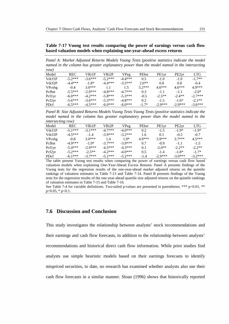
Chapter 7: Direct Cash Flows, Analysts’ Cash Flow Forecasts and Stock Recommendations 231
Table 7-17 Vuong test results comparing the power of earnings versus cash flowbased valuation models when explaining one-year-ahead excess returns
Panel A: Market Adjusted Returns Models Vuong Tests (positive statistics indicate the modelnamed in the column has greater explanatory power than the model named in the intersectingrow)Model REC VRi1P VRi2P VPeg PEhst PE1yr PE2yr LTGVdcf1P -5.2*** -3.6*** -5.2*** -4.4*** 0.5 -1.0 -1.0 -1.7**Vdcf2P -4.4*** -1.8* -4.4*** -3.5*** 2.0** 0.8 0.8 -0.4VPcshg -0.4 3.0*** 1.1 1.5 5.2*** 4.6*** 4.6*** 4.9***Pcfhst -5.5*** -2.9*** -4.8*** -4.7*** 0.3 -1.1 -1.1 -2.0*Pcf1yr -6.0*** -4.2*** -5.8*** -5.3*** -0.5 -2.5** -2.4** -2.7***Pcf2yr -5.6*** -3.6*** -5.3*** -4.8*** 0.2 -1.5 -1.6* -2.1**PDcf -6.5*** -4.5*** -6.0*** -6.0*** -1.7* -2.9*** -2.9*** -3.6***
Panel B: Size Adjusted Returns Models Vuong Tests Vuong Tests (positive statistics indicate themodel named in the column has greater explanatory power than the model named in theintersecting row)Model REC VRi1P VRi2P VPeg PEhst PE1yr PE2yr LTGVdcf1P -5.1*** -3.1*** -4.7*** -4.0*** 0.2 -1.5 -1.9* -1.9*Vdcf2P -4.5*** -1.4 -3.9*** -3.2*** 1.6 0.1 -0.2 -0.7VPcshg -0.8 3.0*** 1.4 1.9* 4.9*** 3.9*** 3.7*** 4.5***Pcfhst -4.9*** -1.9* -3.7*** -3.9*** 0.7 -0.9 -1.1 -1.5Pcf1yr -5.4*** -2.9*** -4.5*** -4.3*** 0.1 -2.0** -2.2** -2.2**Pcf2yr -5.2*** -2.5** -4.2*** -4.0*** 0.5 -1.4 -1.8* -1.7*PDcf -6.1*** -3.7*** -5.1*** -5.2*** -1.4 -2.9*** -3.0*** -3.2***The table present Vuong test results when comparing the power of earnings versus cash flow basedvaluation models when explaining One-Year-Ahead Excess Returns. Panel A presents findings of theVuong tests for the regression results of the one-year-ahead market adjusted returns on the quintilerankings of valuation estimates in Table 7-13 and Table 7-14. Panel B presents findings of the Vuongtests for the regression results of the one-year-ahead quartile size adjusted returns on the quintile rankingsof valuation estimates in Table 7-15 and Table 7-16.See Table 7-4 for variable definitions. Two-tailed p-values are presented in parentheses. *** p<0.01, **p<0.05, * p<0.1.
7.6 Discussion and Conclusion
This study investigates the relationship between analysts’ stock recommendations and
their earnings and cash flow forecasts, in addition to the relationship between analysts’
recommendations and historical direct cash flow information. While prior studies find
analysts use simple heuristic models based on their earnings forecasts to identify
mispriced securities, to date, no research has examined whether analysts also use their
cash flow forecasts in a similar manner. Sloan (1996) shows that historically reported
Chapter 7: Direct Cash Flows, Analysts’ Cash Flow Forecasts and Stock Recommendations 232
cash flows provide investors with valuable information to identify mispriced stocks.
Moreover, while forecasting both earnings and cash flows is a relatively new and
growing trend among analysts, DeFond and Hung (2003) find that analysts cash flow
forecasts provide value relevant information to investors. Accordingly, this study
predicts that analysts’ cash flow forecasts should provide analysts and investors with
useful information to identify mispriced securities.
Currently, the IASB and FASB have both proposed to mandate the use of direct cash
flow statements as part of their convergence project. This proposal has generated much
debate around the associated costs and benefits of reporting direct cash flow statements,
with financial analysts being one of the main proponents of this approach. 63% of
surveyed analysts agreed or strongly agreed that direct cash flow statements provided
them with more useful information for forecasting future cash flows than an indirect
cash flow statement (CFA Institute, 2009). Further, prior studies show information from
direct cash flow statements is value relevant (Clinch et al., 2002), and helps improve the
accuracy of cash flow and earnings predictions (Krishnan and Largay III, 2000; Arthur
et al., 2010). Accordingly, this study also predicts that historical direct cash flow
information will provide analysts with useful information when issuing their stock
recommendations.
Confirming the findings of prior studies, the results show a positive (negative)
relationship between analysts’ stock recommendations and heuristics (residual income
valuation) models based on their earnings forecasts. In contrast, but also consistent with
prior research, the results show a positive (negative) relationship between excess annual
stock returns and residual income valuation (heuristics) models based on analysts’
earnings forecasts. Taken together, these results show that analysts’ earnings forecasts
Chapter 7: Direct Cash Flows, Analysts’ Cash Flow Forecasts and Stock Recommendations 233
provide useful information to help identify mispriced securities, but only when used in
multi-period valuation models. Although analysts appear to use their earnings forecasts
in simple heuristics when issuing their stock recommendations, buy-and-hold investors
fail to earn excess annual stock returns when following these recommendations or
heuristic models.
Investigating the usefulness of analysts’ cash flow forecasts and direct cash flow
information, the chapter demonstrates a positive (negative) relationship between
analysts’ stock recommendations and heuristics (discounted cash flow valuation)
models based on their cash flow forecasts. Moreover, this chapter demonstrates a
positive relationship between analysts’ stock recommendations and the heuristic based
on historical direct cash flows. Analysts not only disregard the results of multi-period
residual income valuation models, they also disregard the results of discounted cash
flow models, when setting their recommendations. Consequently, buy-and-hold
investors are better off using analysts’ cash flow forecasts in multi-period discounted
cash flow models to identify mispriced securities compared to relying on their stock
recommendations. Moreover, compared to the profitability of using residual income
valuation models, the results demonstrate that buy-and-hold investors can earn
significantly higher excess annual returns by identifying mispriced stocks using
discounted cash flow techniques based on analysts’ cash flow forecasts.
Overall, the results not only support the usefulness of analysts’ earnings forecasts,
but they also provide the first empirical evidence of the usefulness of analysts’ cash
flow forecasts when identifying mispriced securities. Moreover, they provide the first
evidence that analysts find direct cash flow information useful when issuing their stock
recommendations, which may be added to the findings from the growing number of

Chapter 7: Direct Cash Flows, Analysts’ Cash Flow Forecasts and Stock Recommendations 234
papers investigating the usefulness of direct cash flow statements. However, consistent
with prior studies, analysts apparently fail to use their forecasts in multi-period
valuation models, rather relying on simple valuation heuristics when identifying
mispriced securities. Consequently, based on buy-and-hold investors’ potential to earn
excess annual returns, analysts fail to identify correctly mispriced securities. To earn the
greatest excess annual returns, buy-and-hold investors should make use of analysts’
forecasts in multi-period valuation models to identify mispriced securities, particularly
analysts’ cash flow forecasts.
Chapter 8: Conclusion 235
8Conclusion
8.1 Background to the Thesis
The International Accounting Standards Board (IASB) and the Financial Accounting
Standards Board (FASB) are currently proposing that direct cash flow statements
should become mandatory for all firms under their harmonised cash flow reporting
requirements. While the IASB and FASB are yet to make a decision on the mandatory
use of direct cash flow statements, if it is decided that only direct cash flow statements
are to be allowed, such a decision would affect cash flow reporting across most of the
world. To date, however, whilst prior empirical studies show strong evidence for the
usefulness of direct cash flow statements, no research has examined whether this still
holds under IFRS. Given the significant changes made to financial reporting with the
introduction of IFRS, before a decision is made to mandate direct cash flow statements,
the IASB and FASB should understand whether direct cash flow statements are useful
in an IFRS reporting framework.
The purpose of this thesis was, therefore, to understand whether or not direct cash
flow statements are useful sources of information in an IFRS reporting environment. To
undertake this analysis, this thesis examined direct cash flow statements in Australia
before and after IFRS adoption. Australia was chosen specifically as one of the few
countries where the reporting of direct cash flow statements was mandatory, and the
early adoption of IFRS was prohibited.
Chapter 8: Conclusion 236
To examine the usefulness of direct cash flow statements in an IFRS environment,
this thesis examined three research questions. In doing so, this thesis provides the first
evidence as to whether the proposed mandating of direct cash flow statements may
improve the informational environment under IFRS. The three research questions are: (i)
Are direct cash flow statements value relevant under IFRS? (ii) Do financial analysts
use information from direct cash flow statements when forecasting cash flows and is
this information more useful under IFRS? (iii) Do financial analysts use information
from direct cash flow statements when issuing their stock recommendations?
8.2 Summary of Findings
8.2.1 Direct Cash Flow Statements Increase in Value Relevance under IFRS
Chapter 5 provides strong evidence that direct cash flow statements are a value relevant
disclosure under both Australian GAAP (AGAAP) and IFRS for both industrial and
extractive firms. Moreover, and fundamentally for answering the overarching research
question of this thesis, for industrial firms the findings reveal that there has been an
increase in the value relevance of direct cash flows since the adoption of IFRS. In
addition, ‘core’ and ‘non-core’ cash flow disclosures are found to increase in value
relevance for industrial firms under IFRS. Consequently, if the IASB were to mandate
direct cash flow statements it would, in all likelihood, provide users of accounts with a
valuable incremental source of information.
The observed increase in value relevance for industrial firms under IFRS is also
consistent with increased uncertainty around the accounting numbers that are being
disclosed. Based upon the evidence of Bissessur and Hodgson (2011), the move to IFRS
created a degree of uncertainty in the accounting numbers being disclosed. In particular,
Chapter 8: Conclusion 237
and consistent with Chalmers et al. (2010), for industrial firms, the findings provides
evidence that IFRS has resulted in a loss of value relevant information regarding
intangibles. As a result, an increase in the value relevance of direct cash flow numbers
is unsurprising in times of uncertainty.
8.2.2 Direct Cash Flow Statements Provide Financial Analysts Useful
Information for Forecasting Cash Flows
Chapter 6 provides strong evidence that financial analysts use information from direct
cash flow statements when estimating future cash flows under both AGAAP and IFRS,
but more so since the adoption of IFRS. Moreover, there is a significant improvement in
the accuracy of analysts’ cash flow predictions post-IFRS, which is likely a result of
financial analysts finding information about direct cash flow components significantly
more useful under IFRS.
Taken together, these findings support opinions of analysts that the information in a
direct cash flow statement is useful when estimating future cash flows, and are
consistent with IFRS improving analysts’ information environment. By requiring the
use of direct cash flow statements, FASB and the IASB would be providing financial
analysts with useful information, which in turn would provide investors with more
accurate cash flow predictions on which to base their investment decisions.
8.2.3 Direct Cash Flow Statements Provide Financial Analysts and Buy-and-
Hold Investors Useful Information to Identify Mispriced Securities
The final empirical chapter starts by showing that, consistent with prior studies, analyst
earnings forecasts provide useful information to help identify mispriced securities when
used in multi-period valuation models. By adapting these models, Chapter 7 further
Chapter 8: Conclusion 238
shows that, when used in discounted cash flow valuation models, analyst cash flow
forecasts provide useful information to help identify mispriced stocks. However,
consistent with prior studies, analysts seemingly fail to use these multi-period valuation
models, relying rather on simple valuation heuristics to identify mispriced securities.
While financial analysts do use their earnings forecasts, cash flow forecasts, and direct
cash flow information, when setting their stock recommendations, buy-and-hold
investors are better off identifying mispriced securities by using multi-period valuation
models. Moreover, compared to the profitability of using residual income valuation
models, the results demonstrate that buy-and-hold investors can earn significantly
higher excess annual returns by identifying mispriced stocks using discounted cash flow
techniques based on analysts’ cash flow forecasts.
Overall, the results provide the first empirical evidence of how analysts’ cash flow
forecasts can provide useful information to identify mispriced securities when used in
discounted cash flow valuation models. Moreover, they provide the first evidence that
financial analysts do use direct cash flow information when issuing their stock
recommendations.
8.3 Policy Implications and Direction for Further Research
In sum, these results provide strong support for the current IASB/FASB proposal to
mandate the use of direct cash flow statements and are consistent with IFRS improving
the quality of the accounting information environment. Given that, to date, the IASB
and FASB have no empirical evidence of the usefulness of direct cash flow statements
under IFRS, this thesis presents a valuable contribution towards the on-going debate of
whether direct cash flow statements should be a mandatory reporting requirement.
Chapter 8: Conclusion 239
While this thesis shows that analysts use information from direct cash flow
statements when forecasting future cash flows, both under AGAAP and under IFRS,
there is further scope to examine the predictive power of direct cash flow components
by using random walk models. Prior studies have found direct cash flow components
increase the accuracy and predictive power of random walk models, but to date these
studies have been conducted on samples where disclosure is solely under local GAAP.
Given the significant changes brought about since the adoption of IFRS, a direction for
further research would be to examine the accuracy and predictive power of direct cash
flow components using random walk models under IFRS. Moreover, while this thesis
used a variety of metrics to evaluate the usefulness of direct cash flow statements, there
is scope for additional research to consider further metrics, such as stock returns and
analysts’ target prices, when evaluating the usefulness of direct cash flow information
under IFRS.
One further factor that must be acknowledged is the sample period of the study, as it
includes one of the biggest periods of uncertainty in recent times, namely the financial
crisis. As a result, a continued reliance on direct cash flow numbers is unsurprising in
such volatile times as it would be logical to assume that users of financial information
focus on the ‘hard’ numbers in the annual report more when making investment
decisions. Whether the usefulness of direct cash flow numbers persists beyond the
current market turmoil would merit investigation in the future. Despite this, the findings
in this thesis present strong evidence that direct cash flow disclosures are useful in an
IFRS reporting environment and provide users of financial accounts with a valuable
source of incremental information.
Bibliography 240
Bibliography
AASB 107. 2009. Australian Accounting Standards. In: Australian Accounting
Standards Board (ed.) Accounting Standard AASB 107: Statement of Cash Flows.
Melbourne: Australian Accounting Standards Board.
AASB 1026. 1991. Australian Accounting Standards. In: Australian Accounting
Standards Board (ed.) Accounting Standard AASB 1026: Statement of Cash
Flows. Melbourne: Australian Accounting Standards Board.
Aharony, J., Barniv, R. & Falk, H. 2010. The Impact of Mandatory IFRS Adoption on
Equity Valuation of Accounting Numbers for Security Investors in the EU.
European Accounting Review, 19, 535-578.
Armstrong, C. S., Barth, M. E., Jagolinzer, A. D. & Riedl, E. J. 2010. Market Reaction
to the Adoption of IFRS in Europe. The Accounting Review, 85, 31-61.
Arnold, J. & Moizer, P. 1984. A Survey of the Methods Used by UK Investment
Analysts to Appraise Investments in Ordinary Shares. Accounting and Business
Research, 14, 195-207.
Arthur, N., Cheng, M. & Czernkowski, R. 2010. Cash Flow Disaggregation and the
Prediction of Future Earnings. Accounting & Finance, 50, 1-30.
Arthur, N. & Chuang, G. C.-H. 2008. IAS 7 Alternative Methods of Disclosing Cash
Flow from Operations: Evidence on the Usefulness of Direct Method Cash Flow
Disclosures. The University of Sydney, Working Paper.
Bibliography 241
Ashbaugh, H. & Pincus, M. 2001. Domestic Accounting Standards, International
Accounting Standards, and the Predictability of Earnings. Journal of Accounting
Research, 39, 417-434.
Asquith, P., Mikhail, M. B. & Au, A. S. 2005. Information Content of Equity Analyst
Reports. Journal of Financial Economics, 75, 245-282.
Austin, L. M. & Bradbury, M. E. 1995. The Accuracy of Cash Flow Estimation
Procedures. Accounting & Finance, 35, 73-86.
Bae, K.-H., Tan, H. & Welker, M. 2008. International GAAP Differences: The Impact
on Foreign Analysts. The Accounting Review, 83, 593-628.
Bahnson, P. R., Miller, P. B. W. & Budge, B. P. 1996. Nonarticulation in Cash Flow
Statements and Implications for Education, Research and Practice. Accounting
Horizons, 10, 1-15.
Ball, R. 2006. International Financial Reporting Standards (IFRS): Pros and Cons for
Investors. Accounting & Business Research, 36, 5-27.
Ball, R. & Brown, P. 1968. An Empirical Evaluation of Accounting Income Numbers.
Journal of Accounting Research, 6, 159-178.
Barker, R. G. 1999. The Role of Dividends in Valuation Models used by Analysts and
Fund Managers. European Accounting Review, 8, 195-218.
Barniv, R., Hope, O.-K., Myring, M. & Thomas, W. 2009. Do Analysts Practice What
They Preach and Should Investors Listen? Effects of Recent Regulations. The
Accounting Review, 84, 1015-1039.
Bibliography 242
Barniv, R., Hope, O.-K., Myring, M. & Thomas, W. 2010. International Evidence on
Analyst Stock Recommendations, Valuations, and Returns. Contemporary
Accounting Research, 27, 1131-1167.
Barth, M. E., Beaver, W. H. & Landsman, W. R. 2001a. The Relevance of the Value
Relevance Literature for Financial Accounting Standard Setting: Another View.
Journal of Accounting and Economics, 31, 77-104.
Barth, M. E. & Clinch, G. 1998. Revalued Financial, Tangible, and Intangible Assets:
Associations with Share Prices and Non-Market-Based Value Estimates.
Journal of Accounting Research, 36, 199-233.
Barth, M. E. & Clinch, G. 2009. Scale Effects in Capital Markets-Based Accounting
Research. Journal of Business Finance & Accounting, 36, 253-288.
Barth, M. E., Cram, D. P. & Nelson, K. K. 2001b. Accruals and the Prediction of Future
Cash Flows. The Accounting Review, 76, 27-58.
Barth, M. E. & Hutton, A. P. 2004. Analyst Earnings Forecast Revisions and the Pricing
of Accruals. Review of Accounting Studies, 9, 59-96.
Barth, M. E., Landsman, W. R. & Lang, M. H. 2008. International Accounting
Standards and Accounting Quality. Journal of Accounting Research, 46, 467-
498.
Beaver, W. H. & Dukes, R. E. 1972. Interperiod Tax Allocation, Earnings Expectations,
and the Behavior of Security Prices. The Accounting Review, 47, 320-332.
Beaver, W. H., Griffin, P. A. & Landsman, W. R. 1982. The Incremental Information
Content of Replacement Cost Earnings. Journal of Accounting and Economics,
4, 15-39.
Bibliography 243
Belkaoui, A. R. & Jones, S. 1996. Accounting Theory, Marrickville, NSW, Harcourt
Brace & Company.
Bernard, V. L. & Stober, T. L. 1989. The Nature and Amount of Information in Cash
Flows and Accruals. The Accounting Review, 64, 624-652.
Beuselinck, C., Joos, P., Khurana, I. & Van der Meulen, S. 2009. Mandatory Adoption
of IFRS and Stock Price Informativeness. SSRN eLibrary. Available at:
http://ssrn.com/abstract=1381242.
Bissessur, S. & Hodgson, A. 2011. Stock Market Synchronicity – An Alternative
Approach to Assessing the Information Impact of Australian IFRS. Accounting
& Finance, 52, 187-212.
Block, S. B. 1999. A Study of Financial Analysts: Practice and Theory. Financial
Analysts Journal, 55, 86-95.
Bond, D., Bugeja, M. & Czernkowski, R. 2012. Did Australian Firms Choose to Switch
to Reporting Operating Cash Flows Using the Indirect Method? Australian
Accounting Review, 22, 18-24.
Bowen, R. M., Burgstahler, D. & Daley, L. A. 1986. Evidence on the Relationships
Between Earnings and Various Measures of Cash Flow. The Accounting Review,
61, 713-725.
Bowen, R. M., Burgstahler, D. & Daley, L. A. 1987. The Incremental Information
Content of Accrual Versus Cash Flows. The Accounting Review, 62, 723-747.
Bradbury, M. 2011. Direct or Indirect Cash Flow Statements? Australian Accounting
Review, 21, 124-130.
Bibliography 244
Bradshaw, M. T. 2002. The Use of Target Prices to Justify Sell-Side Analysts' Stock
Recommendations. Accounting Horizons, 16, 27-41.
Bradshaw, M. T. 2004. How Do Analysts Use Their Earnings Forecasts in Generating
Stock Recommendations? The Accounting Review, 79, 25-50.
Brown, C. D. 1971. The Internal Shift from Balance Sheet to Income Statement,
Michigan, Michigan State University.
Brown, L. D. 1993. Earnings Forecasting Research: Its Implications for Capital Markets
Research. International Journal of Forecasting, 9, 295-320.
Bryant, J. V. 1984. Proposed: A New Statement of Changes. Management Accounting,
49-52.
Byard, D., Li, Y. & Yu, Y. 2011. The Effect of Mandatory IFRS Adoption on Financial
Analysts’ Information Environment. Journal of Accounting Research, 49, 69-96.
Byrd, D. B. & Byrd, S. D. 1986. Using the SCFP. Journal of Small Business
Management, 24, 31-38.
Call, A. 2008. Analysts' Cash Flow Forecasts and the Predictive Ability and Pricing of
Operating Cash Flows. SSRN eLibrary. Available at:
http://ssrn.com/paper=1362177.
Call, A., Chen, S. & Tong, Y. 2009. Are Analysts' Earnings Forecasts More Accurate
When Accompanied by Cash Flow Forecasts? Review of Accounting Studies, 14,
358-391.
Bibliography 245
Call, A., Chen, S. & Tong, Y. 2012. Are Analysts’ Cash Flow Forecasts Naïve
Extensions of Their Own Earnings Forecasts? Contemporary Accounting
Research, Forthcoming.
Camfferman, K. & Zeff, S. 2007. 'Compromise to Harmonise': Setting the IASC's Early
Standards. Financial Reporting and Global Capital Markets - A History of the
International Accounting Standards Committee, 1973-2000. New York: Oxford
University Press.
CFA Institute 1964. The Statement of Source and Application of Funds. Financial
Analysts Journal, 20, 13-16.
CFA Institute. 2009. CFA Institute Member Poll: Cash Flow Survey. Charlottesville:
CFA Institute: Centre for Financial Market Integrity.
Chalmers, K., Clinch, G., Godfrey, J. M. & Wei, Z. 2010. Intangible Assets, IFRS, and
Analysts Earnings Forecasts. SSRN eLibrary. Available at:
http://ssrn.com/paper=1722937.
Cheng, C. S. A. & Hollie, D. 2008. Do Core and Non-Core Cash Flows from
Operations Persist Differentially in Predicting Future Cash Flows? Review of
Quantitative Finance and Accounting, 31, 29-53.
Christie, A. A., Kennelley, M. D., William King, J. & Schaefer, T. F. 1984. Testing for
Incremental Information Content in the Presence of Collinearity. Journal of
Accounting and Economics, 6, 205-217.
Clark, R. S. 1983. Statement of Changes in Need of a Change. CA Magazine, 26-30.
Clinch, G., Sidhu, B. & Sin, S. 2002. The Usefulness of Direct and Indirect Cash Flow
Disclosures. Review of Accounting Studies, 7, 383-404.
Bibliography 246
Coker, J. L. 1986. What Balance Sheets Actually Tell You. Credit and Financial
Management, 88, 22-24.
Companies Act. 1967. Companies Act 1967. In: British Parliament (ed.) Chapter 81.
London: Sir Percy Faulkner, K.B.E., C.B.
Cotter, J., Tarca, A. & Wee, M. 2012. IFRS Adoption and Analysts’ Earnings Forecasts:
Australian Evidence. Accounting & Finance, 52, 395–419.
Cox, P. & Pendersen, T. 2002. Regulation (EC) No 1606/2002 of The European
Parliament and of The Council of 19 July 2002 on the Application of
International Accounting Standards. In: The European Parliament and The
Council Of The European Union (ed.) Regulation (EC) No 1606/2002. Brussels.
Daske, H. & Gebhardt, G. 2006. International Financial Reporting Standards and
Experts' Perceptions of Disclosure Quality. Abacus, 42, 461-498.
Daske, H., Hail, L., Leuz, C. & Verdi, R. 2008. Mandatory IFRS Reporting Around the
World: Early Evidence on the Economic Consequences. Journal of Accounting
Research, 46, 1085-1142.
Davies, M., Paterson, R. & Wilson, A. 1994. Cash Flow Statements. UK GAAP:
Generally Accepted Accounting Practice In The United Kingdom. 4th ed.
Basingstoke: Macmillan Press Ltd.
Dechow, P. M. 1994. Accounting Earnings and Cash Flows as Measures of Firm
Performance : The Role of Accounting Accruals. Journal of Accounting and
Economics, 18, 3-42.
Dechow, P. M., Kothari, S. P. & L. Watts, R. 1998. The Relation Between Earnings and
Cash Flows. Journal of Accounting and Economics, 25, 133-168.
Bibliography 247
DeFond, M. & Hung, M. 2003. An Empirical Analysis of Analysts’ Cash Flow
Forecasts. Journal of Accounting and Economics, 35, 73-100.
DeFond, M. & Hung, M. 2007. Investor Protection and Analysts’ Cash Flow Forecasts
Around the World. Review of Accounting Studies, 12, 377-419.
Deloitte. 2005. A-IFRS vs IFRS: Differences Between Australian Equivalents to
International Financial Reporting Standards (A-IFRS) and International
Financial Reporting Standards (IFRS). Sydney: Deloitte Touche Tohmatsu.
Deloitte. 2009. International Financial Reporting Standards: Model Financial
Statements 2009. London: The Creative Studio at Deloitte.
Deloitte. 2010. Summaries of International Financial Reporting Standards. IAS 7
Statement of Cash Flows: History of IAS 7. 2010. Available at:
http://www.iasplus.com/standard/ias07.htm.
Demirakos, E. G., Strong, N. C. & Walker, M. 2004. What Valuation Models Do
Analysts Use? Accounting Horizons, 18, 221-240.
Donleavy, G. 1992. The Funds Statement: An Inquest. Managerial Finance, 18, 27-44.
Donleavy, G. D. 1994. Cash Flow Accounting: International Uses and Abuses, London
and New York, Routledge.
Drtina, R. & Largay III, J. 1985. Pitfalls in Calculating Cash Flow From Operations.
The Accounting Review, 60, 314-326.

Bibliography 248
Durnev, A., Morck, R., Yeung, B. & Zarowin, P. 2003. Does Greater Firm-Specific
Return Variation Mean More or Less Informed Stock Pricing? Journal of
Accounting Research, 41, 797-836.
Edwards, J. R. 1996. Financial Accounting Practice 1600-1970: Continuity and Change.
In: Lee, T. A., Bishop, A. & Parker, R. H. (eds.) Acccounting History from the
Renaissance to the Present. New York and London: Garland Publishing, Inc.
Ernst & Young. 2005. The Impacts of AIFRS on Australian Companies: A Study of the
Financial Statement Disclosures by Australia’s Top 100 Listed Companies.
Ernst & Young Australia.
Farshadfar, S. 2008. An Investigation of the Relative and Incremental Predictive Ability
of Accrual- and Cash-Based Accounting Measures for Future Cash Flows:
Australian Evidence. Doctor of Philosophy Doctoral Thesis, Griffith University
Business School.
Farshadfar, S. & Monem, R. 2012. The Usefulness of Operating Cash Flow and Accrual
Components in Improving the Predictive Ability of Earnings: A Re-Examination
and Extension. Accounting & Finance, Forthcoming.
Farshadfar, S. & Monem, R. 2013. Further Evidence on the Usefulness of Direct
Method Cash Flow Components for Forecasting Future Cash Flows. The
International Journal of Accounting, 48, 111-133.
FASB. 1978. Statement of Financial Accounting Concepts,. In: Financial Accounting
Standards Board (ed.) No. 1 Objectives of Financial Reporting by Business
Enterprises. Stamford: Financial Accounting Standards Board.
Bibliography 249
FASB. 1987. Financial Accounting Standards. In: Financial Accounting Standards
Board (ed.) Statement of Financial Accounting Standards No. 95 Statement of
Cash Flows. Norwalk: Financial Accounting Standards Board.
FASB. 2009. Project: Financial Statement Presentation: Reference Number: 1630-100.
In: Financial Accounting Standards Board (ed.) Preliminary Views on Financial
Statement Presentation: Comment Letters. Norwalk: Financial Accounting
Standards Board.
FASB. 2010. Financial Accounting Series Exposure Draft: Proposed Accounting
Standards Update. In: Financial Accounting Standards Board (ed.) Staff Draft of
an Exposure Draft on Financial Statement Presentation. Newark: Financial
Accounting Standards Board.
Feltham, G. A. & Ohlson, J. A. 1995. Valuation and Clean Surplus Accounting for
Operating and Financial Activities. Contemporary Accounting Research, 11,
689-731.
Fenton-Jones, M. 2003. Tight Schedule on Revised Standards. Australian Financial
Review. Fairfax Media Publications Pty. Limited.
Finger, C. A. 1994. The Ability of Earnings to Predict Future Earnings and Cash Flow.
Journal of Accounting Research, 32, 210-223.
Francis, J. & Schipper, K. 1999. Have Financial Statements Lost their Relevance?
Journal of Accounting Research, 37, 319-352.
FRS 1. 1991. Financial Reporting Standards. In: The Accounting Standards Board (ed.)
Financial Reporting Standard 1: Cash Flow Statements London: The Financial
Reporting Council.
Bibliography 250
FRS 1. 1996. Financial Reporting Standards. In: The Accounting Standards Board (ed.)
Financial Reporting Standard 1 Cash Flow Statements (Revised 1996). London:
The Financial Reporting Council.
Gentry, J. A., Newbold, P. & Whitford, D. T. 1987. Funds Flow Components, Financial
Ratios and Bankruptcy. Journal of Business Finance & Accounting, 14, 595-606.
Givoly, D., Hayn, C. & Lehavy, R. 2009. The Quality of Analysts' Cash Flow Forecasts.
The Accounting Review, 84, 1877–1911.
Goyal, M. K. 2004. A Survey on Popularity of the Direct Method of Cashflow
Reporting. The Journal of Applied Management Accounting Research, 2, 41-52.
Greenberg, R. R., Johnson, G. L. & Ramesh, K. 1986. Earnings versus Cash Flow as a
Predictor of Future Cash Flow Measures. Journal of Accounting, Auditing &
Finance, 1, 266-277.
Gu, Z. & Wu, J. S. 2003. Earnings Skewness and Analyst Forecast Bias. Journal of
Accounting and Economics, 35, 5-29.
Gujarati, D. 1999. Essentials of Econometrics, Singapore, Irwin McGraw-Hill.
Hail, L. & Leuz, C. 2003. International Differences in the Cost of Equity Capital: Do
Legal Institutions and Securities Regulation Matter? The Wharton Financial
Institutions Center.
Hales, J. & Orpurt, S. F. 2012. A Review of Academic Research on the Reporting of
Cash Flows from Operations. SSRN eLibrary. Available at:
http://ssrn.com/paper=2014857.
Bibliography 251
Han, K. H. 1981. The Funds Statement and Cash Flows. SES Journal, 16-21.
Hausman, J. A. 1978. Specification Tests in Econometrics. Econometrica, 46, 1251-
1271.
Heath, L. C. 1978. Let's Scrap the "Funds" Statement. Journal of Accountancy, 146, 94-
103.
Henderson, S., Peirson, G. & Harris, K. 2004. Financial Accounting Theory, Frenchs
Forest, NSW, Pearson Education Australia.
Hodder, L., Hopkins, P. E. & Wood, D. A. 2008. The Effects of Financial Statement
and Informational Complexity on Analysts' Cash Flow Forecasts. The
Accounting Review, 83, 915-956.
Hodgdon, C., Tondkar, R. H., Harless, D. W. & Adhikari, A. 2008. Compliance with
IFRS Disclosure Requirements and Individual Analysts’ Forecast Errors.
Journal of International Accounting, Auditing and Taxation, 17, 1-13.
Holmes, G. 1976. Standardise Funds Statements. Accountancy, 87, 88-94.
Hope, O.-K. 2003. Disclosure Practices, Enforcement of Accounting Standards, and
Analysts' Forecast Accuracy: An International Study. Journal of Accounting
Research, 41, 235-272.
Horton, J., Serafeim, G. & Serafeim, I. 2012. Does Mandatory IFRS Adoption Improve
the Information Environment? Contemporary Accounting Research,
Forthcoming.
Bibliography 252
Hribar, P. & Collins, D. 2002. Errors in Estimating Accruals: Implications for Empirical
Research. Journal of Accounting Research, 40, 105-134.
IASB. 1989. Framework for the Preparation and Presentation of Financial Statements.
In: International Accounting Standards Board (ed.). London: International
Accounting Standards Board.
IASB. 2008. Discussion Paper: Preliminary Views on Financial Statement Presentation.
In: International Accounting Standards Board (ed.). London: International
Accounting Standards Board.
IASB. 2010. International Accounting Standard 7: Statement of Cash Flows. In:
International Accounting Standards Board (ed.). London: International
Accounting Standards Board.
IASC. 1992. International Accounting Standards. In: International Accounting
Standards Committee (ed.) International Accounting Standard 7: Cash Flow
Statements. London: International Accounting Standards Committee.
IASC Foundation. 2009. International Accounting Standards Committee Foundation -
Revised Constitution 1 February 2009. In: International Accounting Standards
Committee Foundation (ed.).
ICAEW 1985. 10 Statements of Source and Application of Funds. Accounting
Standards 1985/86: The Full Texts of All Exposure Drafts and Accounting
Standards Extant at August 1985. London: Institute of Chartered Accountants in
England and Wales.
Imam, S., Barker, R. & Clubb, C. 2008. The Use of Valuation Models by UK
Investment Analysts. European Accounting Review, 17, 503-535.
Bibliography 253
Jones, S. & Finley, A. 2011. Have IFRS Made a Difference to Intra-Country Financial
Reporting Diversity? The British Accounting Review, 43, 22-38.
Jones, S. & Ratnatunga, J. 1997. The Decision Usefulness of Cash-Flow Statements by
Australian Reporting Entities: Some Further Evidence. The British Accounting
Review, 29, 67-85.
Jones, S., Romano, C. A. & Smyrnios, K. X. 1995. An Evaluation of the Decision
Usefulness of Cash Flow Statements by Australian Reporting Entities.
Accounting & Business Research, 25, 115-129.
Jones, S. & Widjaja, L. 1998. The Decision Relevance of Cash-Flow Information: A
Note. Abacus, 34, 204-219.
Ketz, J. E. & Kochanek, R. F. 1982. Funds Flow Statements. Financial Executives, 34-
41.
Ketz, J. E. & Largay III, J. A. 1987. Reporting Income and Cash Flows from Operations.
Accounting Horizons, 1, 9-17.
Klammer, T. P. & Reed, S. A. 1990. Operating Cash Flow Formats: Does Format
Influence Decisions? Journal of Accounting and Public Policy, 9, 217-235.
Krishnan, G. V. & Largay III, J. A. 2000. The Predictive Ability of Direct Method Cash
Flow Information. Journal of Business Finance & Accounting, 27, 215-245.
Kwok, H. 2002. The Effect of Cash Flow Statement Format on Lenders' Decisions. The
International Journal of Accounting, 37, 347-362.
Bibliography 254
Lee, T. A. 1981. A Survey of Accountants' Opinions on Cash Flow Reporting. Abacus,
17, 130-144.
Lennox, C. S., Francis, J. R. & Wang, Z. 2012. Selection Models in Accounting
Research. The Accounting Review, 87, 589-616.
Li, S. 2010. Does Mandatory Adoption of International Financial Reporting Standards
in the European Union Reduce the Cost of Equity Capital? The Accounting
Review, 85, 607-636.
Livnat, J. & Zarowin, P. 1990. The Incremental Information Content of Cash-Flow
Components. Journal of Accounting and Economics, 13, 25-46.
Lorek, K. & Willinger, G. 2009. The Predictive Ability of Statistically-Based Cash-
Flow Models. Northern Arizona University, Working Paper.
Lorek, K. S., Schaefer, T. F. & Willinger, G. L. 1993. Time-Series Properties and
Predictive Ability of Funds Flow Variables. The Accounting Review, 68, 151-
163.
Lorek, K. S. & Willinger, G. L. 1996. A Multivariate Time-Series Prediction Model For
Cash-Flow Data. The Accounting Review, 71, 81-102.
Matolcsy, Z. & Wyatt, A. 2006. Capitalized Intangibles and Financial Analysts.
Accounting & Finance, 46, 457-479.
McEnroe, J. E. 1989. Cash Flow Accounting Revisited: A Note on a Partial Replication
of the Lee Study. Abacus, 25, 55-60.
Bibliography 255
McEnroe, J. E. 1996. An Examination of Attitudes Involving Cash Flow Accounting:
Implications for the Content of Cash Flow Statements. The International
Journal of Accounting, 31, 161-174.
McInnis, J. & Collins, D. W. 2011. The Effect of Cash Flow Forecasts on Accrual
Quality and Benchmark Beating. Journal of Accounting and Economics, 51,
219-239.
Mitchell, J. D., Goh, S. W. & Forman, S. C. 1995. A Note on the Relationship Between
Reported Cash Flow Measures, Ratios and Their Accrual Counterparts.
Accounting & Finance, 35, 47-62.
Moizer, P. & Arnold, J. 1984. Share Appraisal by Investment Analysts—Portfolio vs.
Non-Portfolio Managers. Accounting and Business Research, 14, 341-348.
Neill, J., Schaefer, T., Bahnson, P. & Bradbury, M. 1991. The Usefulness of Cash Flow
Data: A Review and Synthesis. Journal of Accounting Literature, 10, 117-150.
Newey, W. K. & West, K. D. 1987. A Simple, Positive Semi-Definite,
Heteroskedasticity and Autocorrelation Consistent Covariance Matrix.
Econometrica, 55, 703-708.
Ohlson, J. A. 1995. Earnings, Book Values, and Dividends in Equity Valuation.
Contemporary Accounting Research, 11, 661-687.
Orpurt, S. F. & Zang, Y. 2009. Do Direct Cash Flow Disclosures Help Predict Future
Operating Cash Flows and Earnings? The Accounting Review, 84, 893-935.
Patell, J. & Kaplan, R. 1977. The Information Content of Cash Flow Data Relative to
Annual Earnings. Stanford University, Working Paper.
Bibliography 256
Paton, W. A. 1963. The 'Cash-Flow' Illusion. The Accounting Review, 38, 243-251.
Pike, R., Meerjanssen, J. & Chadwick, L. 1993. The Appraisal of Ordinary Shares by
Investment Analysts in the UK and Germany. Accounting & Business Research,
23, 489-499.
Piotroski, J. & Roulstone, B. 2004. The Influence of Analysts, Institutional Investors,
and Insiders on the Incorporation of Market, Industry, and Firm-Specific
Information into Stock Prices. The Accounting Review, 79, 1119-1151.
Pope, P. F. & McLeay, S. J. 2011. The European IFRS Experiment: Objectives,
Research Challenges and Some Early Evidence. Accounting and Business
Research, 41, 233-266.
Previts, G. J., Bricker, R. J., Robinson, T. R. & Young, S. J. 1994. A Content Analysis
of Sell-Side Financial Analyst Company Reports. Accounting Horizons, 8, 55-70.
PriceWaterhouseCoopers. 2005. PwC inform – IFRS/UK Main Differences Indicator. In:
McCann, H. (ed.) IFRS in the UK. PricewaterhouseCoopers LLP.
Rayburn, J. 1986. The Association of Operating Cash Flow and Accruals with Security
Returns. Journal of Accounting Research, 24, 112-133.
Rosen, L. S. & Don, T. D. 1969. "Funds" Statements: A Historical Perspective. The
Accounting Review, 44, 124-136.
Rutherford, B. A. 2007. Financial Reporting in the UK: A History of the Accounting
Standards Committee, 1969-1990, London and New York, Routledge.
Bibliography 257
Savoie, L. M. 1965. The Accounting Principles Board: What It Is, How It Works and
What Its Role in Business Is. Financial Analysts Journal, 21, 53-57.
Schipper, K. 1991. Analysts' Forecasts. Accounting Horizons, 5, 105-121.
Siegel, J. & Simon, A. 1981. The Statement of Changes in Financial Position: A Vital
Clue to a Company's Financial Health. National Public Accountant, 26, 22-26.
Sloan, R. G. 1996. Do Stock Prices Fully Reflect Information in Accruals and Cash
Flows about Future Earnings? The Accounting Review, 71, 289-315.
Smith, A. F. 1985. Funds Flow Statement Revamped. Management Accounting (UK),
63, 25-29.
Smith, R. G. & Freeman, R. J. 1996. Statement of Cash Flows: The Direct Vs. Indirect
Method Debate Continues. Government Finance Review, 12, 17-21.
Soderstrom, N. S. & Sun, K. J. 2007. IFRS Adoption and Accounting Quality: A
Review. European Accounting Review, 16, 675-702.
Spiller, E. & Virgil, R. 1974. Effectiveness of APB Opinion No. 19 in Improving Funds
Reporting. Journal of Accounting Research, 12, 112-142.
Street, D. L. & Shaughnessy, K. A. 1998. The Quest for International Accounting
Harmonization: A review of the Standard Setting Agendas of the IASC, US, UK,
Canada, and Australia, 1973-1997. The International Journal of Accounting, 33,
179-209.
Swanson, E. P. & Vangermeersch, R. 1981. The Statement of Financing and Investing
Activities. CPA Journal, 32-39.
Bibliography 258
Tan, H., Wang, S. & Welker, M. 2011. Analyst Following and Forecast Accuracy After
Mandated IFRS Adoptions. Journal of Accounting Research, 49, 1307-1357.
Tarca, A. 2004. International Convergence of Accounting Practices: Choosing Between
IAS and US GAAP. Journal of International Financial Management &
Accounting, 15, 60-91.
Taylor, P. 1979. Published Funds Statements and SSAP 10. Accountancy, 90, 95-98.
Taylor, S. L. 1987. International Accounting Standards: An Alternative Rationale.
Abacus, 23, 157-170.
Thomas, B. S. 1982. Reporting Cash Flow Information. Journal of Accountancy, 154,
98-108.
Trout, R. K., Tanner, M. M. & Nicholas, L. 1993. On Track with Direct Cash Flow.
Management Accounting, 75, 23-27.
Tsalavoutas, I., André, P. & Evans, L. 2012. The Transition to IFRS and the Value
Relevance of Financial Statements in Greece. The British Accounting Review, 44,
262-277.
Vuong, Q. H. 1989. Likelihood Ratio Tests for Model Selection and Non-Nested
Hypotheses. Econometrica, 57, 307-333.
Wahlen, J. & Wieland, M. 2011. Can Financial Statement Analysis Beat Consensus
Analysts’ Recommendations? Review of Accounting Studies, 16, 89-115.
Bibliography 259
Walker, R. G. & Robinson, S. P. 1994. Competing Regulatory Agencies With
Conflicting Agendas: Setting Standards For Cash Flow Reporting In Australia.
Abacus, 30, 119-139.
Wallace, R. S. O., Choudhury, M. S. I. & Pendlebury, M. 1997. Cash Flow Statements:
An International Comparison of Regulatory Positions. The International Journal
of Accounting, 32, 1-22.
White, H. 1980. A Heteroskedasticity-Consistent Covariance Matrix Estimator and a
Direct Test for Heteroskedasticity. Econometrica, 48, 817-838.
Wilson, G. P. 1986. The Relative Information Content of Accruals and Cash Flows:
Combined Evidence at the Earnings Announcement and Annual Report Release
Date. Journal of Accounting Research, 24, 165-200.
Wilson, G. P. 1987. The Incremental Information Content of the Accrual and Funds
Components of Earnings After Controlling for Earnings. The Accounting Review,
62, 293-322.
Yang, Y. 2010. Mandatory IFRS Reporting and Analysts’ Information. Queen’s
University Belfast, Working Paper.
Yap, C. 1994. Cash Flow Statements: The Australian Experience. Advances in
International Accounting, 6, 165-183.