Embed Size (px)
Citation preview

O'*ernment AccelltOn No.
89-1203-lF
itle
ing Orgoni zotion Hom• ond Addr•u
The University of Texas at Arlington Arlington, TX 76019
Sponaor~nt Ag•ncy Home ond Adclrns
Texas State Department of Highways & Public Transportation, D-10 Research P. o. Box 5051, Austin, TX 78763
S~o~pplem•ntory Note 1
Performing Orgo11iaotion epott No.
1203-lF
Final
Study done in cooperation with u.s. Dept. of Transportation, Federal Highway Administration
This project was initiated to investigate the profile measuring capabilof the Siometer or (Walker self-calibrating process) so that it might be for various profile measuring applications. Since the Siometer is capa
of providing pavement profile estimates, it was desired to determine how losely these estimates were to actual profile, or to profile measurements
by the Surface Dynamics Profilometer (SOP) owned by the State. For the study, profile data from the Siometer was compared to that from
SDP for the same sections. From the results of the study the self-caliting process does a good job of measuring the longer profile wavelengths
t eight feet and greater). The shorter wavelengths are somewhat attenuat-
implement the acceleration only, and South a processes for measuring profiles and rutting. The acoustic sensor
s better estimates of the shorter wavelengths which could also make the more suitable for profile measurements.
Dynamics Profilometer (SDP) Lasers, Probes, Pavement
iceability Index (PSI), Siometer
18. Distribution
No restrictions. This document is available to the public through the National Technical Information Service, Springfield, VA. 22161
rily Cloud, (of this Security Clouif. (of this ogn 22. Pric•
Unclassified 53
F 1700.7 I8•UI


USE OF THE SIOMETER FOR PROFILE MEASUREMENTS
by
Roqer s. Walker
The university of Texas at Arlinqton
Research Report 1203-1F
Research Project 8-18-89-1203
conducted for
Texas State Department of Hiqhways and Public Transportation
in cooperation with the u.s. Department of Transportation
Federal Hiqhway Administration
March 1991


.... .... ....
s.,. ....
.. ft
•• .,;
.,.a ttl ,,z .,;Z
01'
lb
Itt> Tbop 1101'
" pC
qt pi Ill ydl
..
Appreaimate Comrartions to Metric: Measarts
.... , .. ~~._
"'""'"' ·ylfds .......
__ .......,. ~~~-·-ylfds _ ... n •• -· ......., .. pounde 1lhOft lOllS
12000 lilt
.. _ bb..._. lltoid CIIIIOe .. .. _ pi•• qv..ts
"""..,• cubic'"' cubic ylfds
Mohitly •r lENGTH
*2.5 30 0.1 1.1
AREA
1.& 0.05 0.1 2.1 o.•
MASS (-ilhlt
21 0.41 o.s
VOLUME
II 111 30 0.24 0.47 0.11 J.l O.OJ 0.11
TEMPERATURE fam1J
, ............ . ....._ ..... . 11/!llaiW . -.... ... " 321
To Fin
anti...._• c ......... -· .............
--..-·-· ............. ~~~---· -··· .. ·-..........
-lli._ -· mill lilt•• milliliters milliliter• ...... ..... .... ,. liters cubic,..••• cubic ........
c ....... ._. ......
s.,.. ••
""' Clll
"' .....
_, ..,z ,jl ..,._2 ...
I
•• '
"'' "'' ....
I
"" .,,
•t:
•t '" • l.5f le•acttyt. fur olh4tr ••-=t conwM•tOt'S .,_.,..,... •'••led t.:tbtes .... NIS MtiiC,. Pubf.liS. Uornu of .. •Qhtl •rd ....._..... ,_..c. IZ.25. SO CataloG No.. Cll .. tO:ll!ll,
METRIC CONVERSION FACTORS
..
. -
.. -
..
..
..
...
..
I
=
= = E =-= ;; = =-E
==
.. .. .. .. ;;
a
l!:
= ~
= = ~
!!
!!
--.. .. ... • .. .. ...
==----= .. .. ..
a • = 6
s, .... ,
""" ""' m m ....
""' ,.a .,.z
""'
I .. ....
I
"" "'l
•t:
Approxl••te Conursioos from Metric: Measuyu ..... , .. ~~. ... lllllli-· _,.,._. ---Ill !aNt••
_a...,lilllelors ---· -•i-s hectaNaC10.000m'l
••lliply .,
lENGTH
0.04 0.4 l.J 1.1 0.1
AREA
e.111 u ••• 2.1i
MASS l-ight)
1•llilogr-
-··1000 lltl
llllllillt••
"-litera litwa cubic-• CW!c-•
0.035 2.2 1.1
VOLUME
O.OJ 2.1 1.011 0.21
35 1.3
TEMPERATURE (erttl)
C.l•iu• -- IISII!IM -121
h fi••
tndte~
'n(;ho:l
feet yams miles
-.q...,... tnchel SqU.ara yards square mite~ ......
ounces
-d• !Jh()ll1 .,.$
tiUoid ounces pinll quarts
pitons
cub•c. '"' cubic. yafds
fahrenM•t HmpltrratUt'•
•F ., 32 .. :!12
_ .. i . . . ~ . I r? , I I ·~ I ~ I ~~·. , • ·~·. • • ~ ~ f I I I I I J t i J -40 -10 20 40 eo eo too ~ u ~
s, ......
1ft
fl
'"" ....
,z .r ,.,z
o• lb
"01'
Ill ql
1)01 ftJ
ydl
..

The contents of this report reflect the views of the author, who is responsible for the facts and accuracy of the data presented herein. The contents do not necessarily reflect the official views or policies of the Federal Highway Administration. This report does not constitute a standard, specification, or regulation.
There was no invention or discovery conceived or first actually reduced in the course of or under this contract, including any art, method, process, machine, manufacture, design or composition of matter, or any new and useful improvement thereof, or any variety of plant which is or may be patentable under the patent laws of the United States of America or any foreign country.
iv

PREFACE
This project report presents final results from Project B-18-89-1203. The Project was initiated to determine the feasibility of using profile from the Siometer (Walker Roughness Device or WRD). This report discusses the results of profile comparisons of the Biometer with those obtained by the Surface Dynamics Profilometer (SDP).
Special recognition is due David Fink and Jim Wyatt, of D-18, for their support and contributions in the project. Recognition is also due Robert Light of D-18, for his help in collecting Siometer and SOP data. Recognition should also be given to Dr's Emanuel Fernando and Robert L. Lytton of the Texas Transportation Institute for aiding in evaluating the profile data from both the Siometer and SOP. Among other things, they were interested in the use of the profile estimates for computing the dynamic response of trucks to road profile. Finally, recognition is due Weishein Fu, a graduate student at The University of Texas at Arlington. He wrote the profile analysis program described in the Appendix and used for the profile comparisons.
Roger s. Walker
February 1990
v

ABSTRACT
This report provides the final details on Research study 8-18-89-1203. The research was initiated to investigate the profile measuring capability of the Siometer or Walker self-calibrating roughness process. Since the State currently owns twelve of these units and which have primarily been used for obtaining Pavement Serviceability Index measurements for the state's Pavement Management System, it was desired to determine how well the predicted profile estimates followed that of the Surface Dynamics Profilometer (SOP). The results of this study are included in this report.
KEY WORDS: Surface Dynamics Profilometer (SOP), Selcom Lasers Probes, Pavement Serviceability Index (PSI), Siometer.
vi

SUMMARY
This project was initiated to investigate the profile measuring capability of the Siometer or (Walker self-calibrating process) so that it might be used for various profile measuring applications. Since the Siometer is capable of providing pavement profile estimates, it was desired to determine how closely these estimates were to actual profile, or to profile measurements made by the surface Dynamics Profilometer (SDP) owned by the State. currently in the State, pavement roughness is measured in terms of Pavement Serviceability Index or PSI (computed from road profile data obtained by the SOP). PSI provides an indication of the ridability of the pavement to the traveling public. The Siometer has primarily been used to date for estimates of such measurements or SI (a prediction of PSI) for the state's Pavement Management system.
For the study, profile data from the Siometer was compared to that from the SOP for the same sections. From the results of the study the self-calibrating process does a good job of measuring the longer profile wavelengths (about eight feet and greater). The shorter wavelengths are somewhat attenuated. When the Siometer is located in a standard vehicle and measurements made at highway speeds with a single accelerometer, the method does not give the same PSI results as the SOP owned by the State. The Siometer profile measurements will typically yield smaller or smoother PSI measurements when these profiles are run through the PSI program used by the State (Vertac), because of its inability to measure the smaller wavelengths as accurately.
From the results of the study it is concluded that the profile estimates from the Siometer at highway speeds should probably only be used for SI (or IRI) measurements for which the current system is designed. However, from the close results noted when installing the Siometer on the SDP, it might be possible to use the self-calibrating process of the Siometer on a small light weight vehicle or trailer towed by such a vehicle at a much slower speed to more accurately obtain the short wavelength information. The Siometer has been modified to implement the acceleration only, and South Dakota processes for measuring profiles and rutting. The acoustic readings for this process provide better estimates of the shorter wavelengths.
vii

IMPLEMENTATION STATEMENT
The State currently owns a number of the R680 roughness measuring instruments or Siometers. These units are used primarily for providing Pavement Serviceability measurements which are used for the State's Pavement Evaluation system. Since the unit can also provide an estimate of the profile, and recently the implementation of the South Dakota road profile measuring concept, their availability for other purposes would provide the State with a more versatile instrument.
viii

TABLE OF CONTENTS
PREFACE . . . . . . . . v
ABSTRACT . vi
SUMMARY . . . . . . . . . . . . . . . . . . . . . . . . vii
IMPLEMENTATION STATEMENT • . . viii
LIST OF FIGURES X
CHAPTER
I. INTRODUCTION 1
1.1 Background 1
1.2 The Siometer • . • • 2
1.3 The surface Dynamics Profilometer • 3
II. Profile Analysis • 4
2.1 Evaluation of Self-Calibrating Process On the SDP • . • • • • . • • • • • 4
III. CONCLUSIONS AND FURTHER RESEARCH • . • • • . . . 30
REFERENCES • . 33
APPENDIX • • 34
ix

I
I I I' I'
2.1
2.2
2.3
2.4
2.5
2.6
2.7
2.8
2.9
2.10
2.11
LIST OF FIGURES
Siometer vs. SOP . . . . . . . . . . Power Spectrum - Siometer vs SOP . . . . . . . . Siometer vs SOP - Section 12 (Right Wheel Path)
Siometer vs SOP - Section 1 (Right Wheel Path)
Siometer vs SOP- Section 12 (Average) •.•.
Siometer vs SOP - Short wave Lengths - Sec 12
Siometer vs SOP - Short Wave Lengths - Sec 1
Comparison of Wheel Path Profile - SOP Repeat Runs o • • o • • • • o o o • • •
Comparison of Profile Elevations - Sec 1
Comparison of Profile Elevations - Sec 7
Comparison of Profile Elevations - Sec 40
2o12 Comparison of Profile Elevations - Average
2o13
2.14
Power Spectra Comparison - Sec 1
Power Spectra comparison - Sec 7
2.15 Comparison of Power Spectra Densities
2.16 Correlation Coefficients - Power Spectra
2.17 RMS Deviations - Power Spectra
3.1 SOP Profiles Before And After overlay o
X
5
6
9
10
11
12
13
14
19
20
21
22
24
25
26
28
29
31

CHAPTER 1
INTRODUCTION
1.2 BACKGROUND
This project was initiated to investigate the profile measuring capability of the Siometer or (Walker self-calibrating process) so that it might be used for various profile measuring applications. Since the Siometer is capable of providing pavement profile estimates, it was desired to determine how closely these estimates were to actual profile, or to profile measurements made by the Surface Dynamics Profilometer (SOP) owned by the State. currently in the State, pavement roughness is measured in terms of Pavement Serviceability Index or PSI (computed from road profile data obtained by the SDP). PSI provides an indication of the ridability of the pavement to the traveling public. The siometer has primarily been used to date for estimates of such measurements or SI (a prediction of PSI). for the State's Pavement Evaluation System.
For the study, profile data from the Siometer was compared to that from the SOP for the same sections. At first various signal processing programs were used. However, it soon became apparent, that in order to perform the type of large scale comparisons needed, more easily used analysis software would have to be developed, specifically for road profile data. During this project such profile analysis software has been developed.
This Report provides the comparisons made between the estimated profile obtained by the Siometer with that obtained with the SOP. The Appendix provides a description of the Profile Analysis software developed so that the profile comparisons could easily be accomplished.
1.2 THE SIOMETER
The development of the Siometer was initiated by Or. Roger Walker during the early 1970's. With the high cost of the SOP and the calibration problems of the Mays Ride Meter (MRM), this device was developed as a low cost method for obtaining roughness measurements. A unique feature of this device is the statistical modeling procedure, for characterizing the vehicle in which it is installed. Through this procedure, the influence of the vehicle on the measurement process is identified and removed (1,2). The statistical model is parametrized with the Siometer's on-board microcomputer using vertical accelerations of the vehicle measured at fixed distances as the vehicle is driven down the road. Vertical accelerations are obtained from an accelerometer typi-
1

cally located in the trunk of the vehicle over the rear axle. Once the parameters of the vehicle are determined, the Siometer is said to be "calibrated" and ready for profile measurements. The vehicle is then driven over the roadway sections for which profiles are to be determined and the resulting accelerations are measured. The difference between the actual measurements and those predicted from the statistical model are used to estimate the road profile by integrating the acceleration differences with the equally spaced successive samples.
The primary application of the Siometer within the State is for the evaluation of riding quality. Thus, the device became known as the Siometer since its primary output is the Serviceability Index (SI) even though the SI is calculated using statistics derived from the predicted road profile. The device is portable and can be easily transferred from one vehicle to another.
The current version of the Siometer used by the Texas state Department of Highways and Public Transportation (SDHPT) is the R680 system manufactured by Micro-Sher Incorporated. The system computes and displays serviceability index and predicts the pavement profile.
An enhanced version has recently been implemented with the south Dakota method (Ref 4) of measuring longitudinal profiles. The South Dakota profiler, currently considered by many to be a Class 2 instrument (Ref 5), is becoming a popular device for measuring pavement profiles. This device measures pavement profile elevations by the use of an accelerometer and a acoustic sensor. The acoustic sensor performs the same function as the laser probe in the SDP. The South Dakota profiler differs from the Profilometer in this respect and also in the procedure used for sampling and integrating the accelerometer signal.
Essentially, the method samples and integrates the accelerometer at fixed time increments, rather than at fixed distance intervals before summing with the appropriate vehicle body-road displacements. By using the acoustic sensor for the vehicle-body road displacements in place of the much more expensive laser, an inexpensive profile measuring process can be implemented. Of course the lasers and in particular the method used for computing the profile of the SDP would be more precise. The current version of the South Dakota Profiler measures longitudinal profile elevations at the inner wheel path. It also provides estimates of pavement rutting by two additional sensors. All three sensors and accelerometer are located in the modified front bumper of the vehicle.
Because the Siometer is essentially a portable roughness computer which implements the self-calibrating process, it can easily implement the south Dakota Profiler concept by the simple
2

installation of acoustic sensors and software. As noted, it has recently been upgraded for this purpose. The R680 system will allow up to five acoustic sensors for the rut depth measurements.
1.3 THE SURFACE DYNAMICS PROFILOMETER
The Surface Dynamics Profilometer (Ref 6) or SOP was purchased from K.J. Law (Model 6900) by the State. (The System is similar in design to that originally built by K.J. Law except that the potentiometer/road-following wheel combination has been replaced with two non-contact Selcom laser probes (Ref 7). In addition, the data acquisition and processing capability was upgraded to take advantage of improvements in hardware technology and thus allow data reduction to be conducted in the field. consequently, roughness statistics and profile data can now be obtained as soon as a run is completed on a particular highway segment and the results provided on standard personal computer disk format.
3

I . CHAPTER 2
PROFILE ANALYSIS
2.1 Evaluation of the Self-Calibrating Process
In order to determine the profile measuring capability of the Siometer or self-calibrating process, it was decided to make multiple runs on pavements of different roughness ranges. The pavement roughness ranges would be determined from the PSI values computed from SOP profile. Initially, several runs were made between the SOP and the Siometer. The Siometer was located in different vehicles for the runs. The profile from the Siometer was then used by the PSI program and the PSI compared with that when using profile from the SOP. For most runs, the computed PSI from SOP profile was about 0.4 greater than that of the Siometer profile. That is the Siometer typically would indicate a smoother value. When using the Siometers in the SI mode for PES measurements (Ref 3), the unsealed slope variance of the road is correlated to the corresponding PSI, thus such consistent readings are explained by the regression or correlation procedure. Although the Siometer was typically located in different vehicles, this case seemed to always occur. Thus it was decided to make comparisons other than PSI or IRI so that differences between profiles could be better investigated.
Figure 2.1 illustrates the differences between repeat runs of the Siometer and SOP. The Siometer was installed in one of the State's cars designated for SI measurements. This comparison was typical of what was noted between profiles from the Siometer and SOP. Figure 2.2 illustrates the power spectral density for the two runs. The SOP profile shown in this figure is the average profile between the right and left wheel paths. Recall the Siometer uses a single accelerometer, which is typically located in the center of the vehicle trunk over the axle.
The differences in wheel paths and the location of the accelerometer made it difficult to make close comparisons between profile from the Siometer and that from the SOP. In order to obtain the best comparisons between profile measurements from the two devices, it was decided to sample the same accelerometer data used by the SOP and then to compare the two measurements. Additionally, since the SOP uses two accelerometers, one for the right side and one for the left side, the self-calibrating process was used on both vehicle sides, thus yielding right and left profile estimates.
4

Figure 2.1
PROFILE SEC 40 SIOMETER(P4:0.3) .vs. SDP(N40.1)
1.4
1.2
1
0.8
0.6
- 0.4: II t'J 0.2
fll ~ ~ Ill ..,. II 0 ::! ~
0 ~ -0.2
I.{)
Eot - -0.4
-0.6
-0.8
-1
-1.2
-1.4
0 200 4:00 600 800 1000 1200 1400 1600 1800 2000 2200
DISTANCE - FEET

Figure 2.2
SEC 40
150
140
130
1~0
110
Ill o· 100
It p:j 90
\0
~ 0 11. 90
'10
60
60
40
~ \,
,.., " SOP"- ~ ~-., ""-'-",t ·~------, - - "--~ -., r -""'-" -. ~-:::::::;::__--:---.:::~-:::::-:·'---::::::;:--- ---../ \ ____ __,---~, - ~ 1'"
Siometer
30 . 0 OT1~5 OT~5 OT3'l6 OT5 oT~•rzo O/l5 OYS~ifj 1
PRBQUBNCY CYDLBS PBR POOT

For the evaluation, nine bituminous test sections were selected. They were selected so that there were three pavements each of the rough, medium rough, and smooth categories, as indicated by their respectively PSI. All sections were twotenths miles in length. The serviceability indices calculated from the SOP profiles on the nine selected sections are shown in Table 2.1. All sections, with the exception of TC7 in Tarrant county, are located within the general vicinity of Austin, Texas.
The pavement profiles of the nine sections were measured using each profile measuring method. For each test section, two profile measurements were obtained. Profile elevations were taken at 0.50 ft. intervals along each 0.2 mile section. The same raw acceleration data was used for both the SOP and the Siometer self-calibrating process. This allowed profile measurements to be made simultaneously for each system for any given run. This technique eliminated errors associated with run-to-run variations. Some differences include separate wheel paths and starting times between profile measurements. All measurements were taken at 20 milesjhour in an attempt to traverse the same wheel paths each time a run was made on a particular section. On two of the rough sections (Section 1 and 4), yellow dots painted at regular intervals on the wheel paths were used to guide the path of travel between runs.
In order to establish a benchmark for evaluating Siometer profiles, a comparison of the profiles from repeat runs of the Profilometer was initially made. Figures 2.3 and 2.4 illustrates an overall comparison for the right wheel path (typically the rougher) for a rough and smooth section and was typical for all runs. Figure 2.5 illustrates the differences between the average right and left profiles for the two methods. The figures indicate an excellent agreement between the two methods for the longer wavelengths. Figures 2.6 and 2.7 provide a closeup of what typically was found on the shorter wavelengths. The Siometer process tracks the longer wavelengths however it doesn't have the short wavelength resolution provided by the lasers of the SOP.
The differences between the two profile methods are further examined in Figure 2.8. This figure compares the measured left wheel path profile elevations from repeat runs of the SOP on Section 1 (one of the rougher sections). The correlation coefficient 'r' between the measured profile elevations was determined to be 0.985 as shown in the figure. Similarly, correlation coefficients between measured profile elevations from repeat runs of the SOP on the other test sections were calculated. The results are summarized in Table 2.2.
7

Section
1
4
7
12
21
31
40
42
TC7
Table 2.1. Test Sections
Location Present Serviceability Index (Average two runs)
Decker Lake Road West, 1.87 approximately 0.2 miles west of FM 973
Decker Lake Road East, 1.30 approximately 0.3 miles west of FM 973
u.s. 183 South, 1.5 4.24 miles north of Burleson Road
u.s. 183 North, 1.1 4.57 miles north of Burleson Road at one-way sign at cross-over north of creek
Pearce Lane West, 1.69 approximately 0.9 miles east of FM 973
FM 685 North, approximately 0.2 miles north of Phillips 66 gas station
FM 973 South, 0.56 miles south of Schmidt Lane
FM 3177 South, at Texas Heritage Center sign
u.s. 183 frontage road, west bound, near intersection with U.S. 157, in Tarrant county, north of Arlington
8
2.55
3.06
4.01
3.36

Fi gu r e 2 . 3
Siometer vs SOP Sec 12 Right Wheel Path
----------~~~----~------~ 0.4
0.3
0.2
"' 0.1
UJ QJ ..c u c 0
......_,.
QJ ur ~ Jlll ll~ 'U"', ..R \I ru I ~ I#Ut ll. 1\ r• · ~ l!l\ I "II I (J)
-o :J -0.1 ~ Q.
E <{
-0.2
-0.3
-0.4
- 0.5 ~-~-~-~-_,..-...,...-....... - ....... - ....... --,...-~-_j 0 100 300 400 500 700 800 200 600 900 1000
~ r
Distance (Feet) Siometer -- SOP

!"'. (I] Q) L u c -'-.../ Q)
'"0 :J
;t::
Q
E <(
Figure 2.4
Siometer vs SOP Sec 1 Right Wheel Path
1.6 ~------------------------------------------------------------------~
1.4
1.2
0.8
0.6
0.4
0.2
0
-0.2
-0.4
-0.6
-0.8
- 1
0 100 200 300 400 500 600 700 800 900 1000
Distance (Feet) - Siam.., · "'t -- SDP
0 rl

0.4
0.3
0.2
0.1 ,.,....._
en ClJ
0 ..c u c
..__....
ClJ -0.1 "0 :J
+..1
0.
E -0.2
<(
-0.3
-0.4
-0.5
-0.6 '
0 100
F i g ur e 2 . 5
S io m e t e r vs SO P - Sec 1 2 AVERAGE RIGHT AND LEFT
200 300 400 500 600 700 800
Distance (Feet) Siometer -- SOP
900 1000
.--<
.--<

" 13 J: 0 z v •
Figure 2.6
Siometer vs SOP - SEC 1 2 RIGHT
0.1 ---------------~----------~----------~-------------~-----------
0.08
0.06
0.04
0.02
0~------~--~-------------+-----+-----r---------~~------~~
"g -0.02 .... -Q. ~ -o.04
-0.06
-0.08
-0.1
-0.12 -+----.--------""'f--.--.r---r---+-------T----t-------,r-----t--------r-----1
32 33 34 35 36 37
Distance (Feet) SCP · Siometer
N .-1

,.... 13 ::r: 0 z v
• '0 :::t ..., -"ii ~
-0.1
-0.2
-O.J
-0.41 I \
-0.5
-0.6
Siometer vs SOP - SEC 1 RIGHT
I I ~ I I I I I I
-o. 7 1 1 1 1 1 I• 1 • 1 • 1 1 1 1 1 • 1 • 1 • 1 14.5 15.5 16.5 17.5 18.5 19.5 20.5 21.5 22.5 23.5 24.5
Distance (Feet) SCP Siometer
f") .....

2
t'""t (" 1 c c . '' ., s:. 0 c -v c 0 0 ~
g --" • w
• ..... .._ f -1
D.
-2
' I
I
-2
Figure 2.8
N = 2198 obs r = 0.985
-1 0 1
Profll e Elevatfon (Inc he~. run 1)
Comparison of left wheelpath profile elevations from repeat runs of the PrQf\lometer on Section 1.
I <;I' ...-!
2

...-----1' '
!i!
11:1
I!''' I
il'i .: iii
Section 1
1
4
4
7
7
12
12
21
21
31
31
40
40
42
42
TC7
TC7
Table 2.2 Correlation coefficients between repeat SOP runs
Wheel path Corr. Coef. left 0.985
right 0.967
left 0.983
right 0.976
left 0.936
right 0.936
left 0.890
right 0.866
left 0.987
right 0.952
left 0.973
right 0.980
left 0.961
right 0.969
left 0.956
right 0.935
left 0.833
right 0.869
15
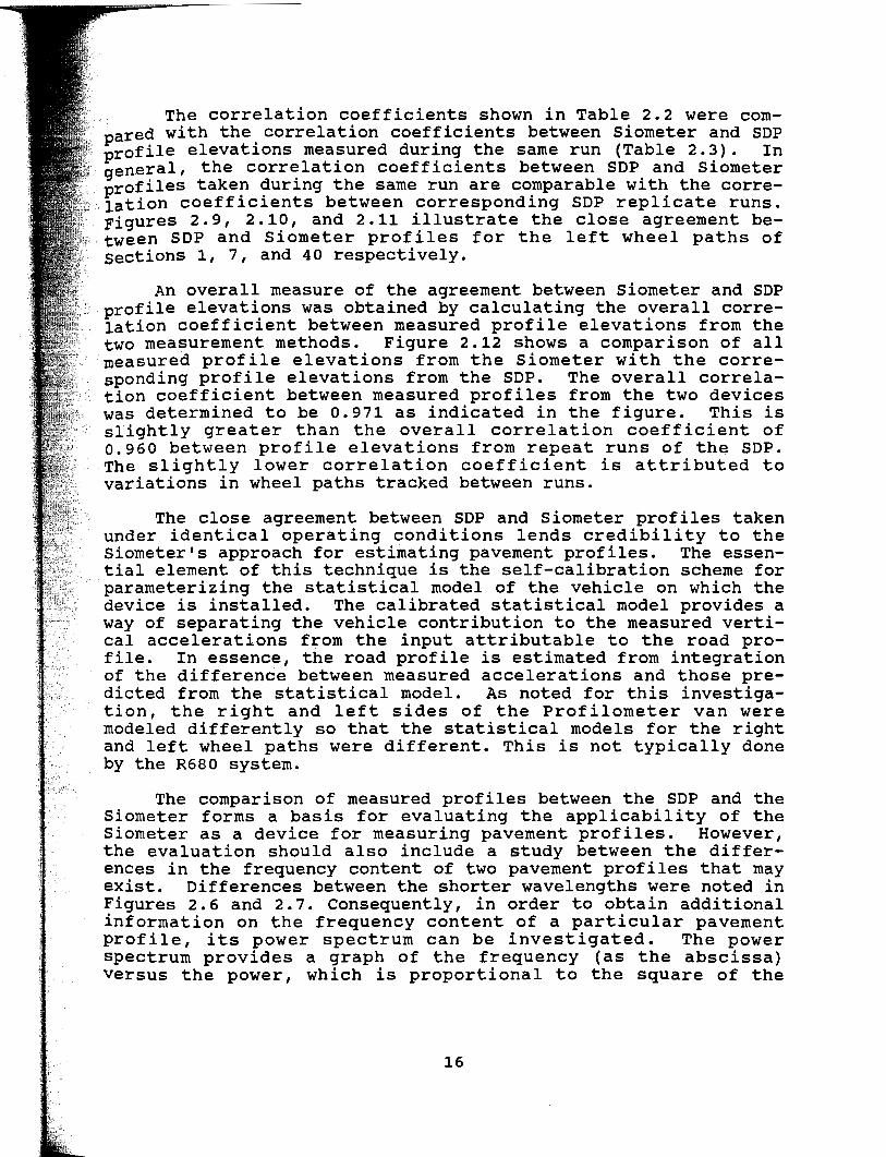
The correlation coefficients shown in Table 2.2 were compared with the correlation coefficients between Siometer and SDP profile elevations measured during the same run (Table 2.3). In general, the correlation coefficients between SDP and Siometer profiles taken during the same run are comparable with the correlation coefficients between corresponding SDP replicate runs. Figures 2.9, 2.10, and 2.11 illustrate the close agreement between SDP and Siometer profiles for the left wheel paths of sections 1, 7, and 40 respectively.
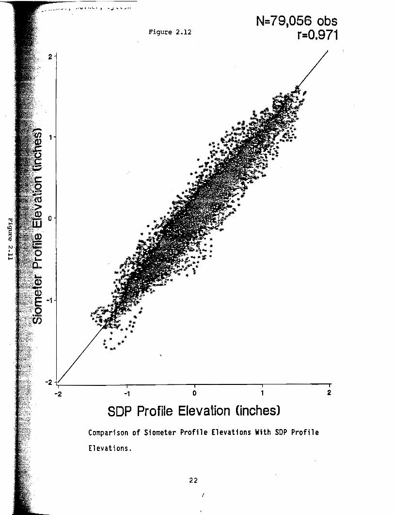
An overall measure of the agreement between Siometer and SDP profile elevations was obtained by calculating the overall correlation coefficient between measured profile elevations from the two measurement methods. Figure 2.12 shows a comparison of all measured profile elevations from the Siometer with the corresponding profile elevations from the SDP. The overall correlation coefficient between measured profiles from the two devices was determined to be 0.971 as indicated in the figure. This is slightly greater than the overall correlation coefficient of 0.960 between profile elevations from repeat runs of the SDP. The slightly lower correlation coefficient is attributed to variations in wheel paths tracked between runs.
The close agreement between SDP and Siometer profiles taken under identical operating conditions lends credibility to the Siometer's approach for estimating pavement profiles. The essential element of this technique is the self-calibration scheme for parameterizing the statistical model of the vehicle on which the device is installed. The calibrated statistical model provides a way of separating the vehicle contribution to the measured vertical accelerations from the input attributable to the road profile. In essence, the road profile is estimated from integration of the difference between measured accelerations and those predicted from the statistical model. As noted for this investigation, the right and left sides of the Profilometer van were modeled differently so that the statistical models for the right and left wheel paths were different. This is not typically done by the R680 system.
The comparison of measured profiles between the SDP and the Siometer forms a basis for evaluating the applicability of the Siometer as a device for measuring pavement profiles. However, the evaluation should also include a study between the differences in the frequency content of two pavement profiles that may exist. Differences between the shorter wavelengths were noted in Figures 2.6 and 2.7. Consequently, in order to obtain additional information on the frequency content of a particular pavement profile, its power spectrum can be investigated. The power spectrum provides a graph of the frequency (as the abscissa) versus the power, which is proportional to the square of the
16

Table 2.3. Correlation coefficients between SOP and Siometer (same run)
Run Section Number Wheel path
1 1 left
1 1 right 0.974
1 2 left 0.987
1 2 right 0.975
4 1 left 0.967
4 1 right 0.972
4 2 left 0.968
4 2 right 0.963
7 1 left 0.977
7 1 right 0.974
7 2 left 0.980
7 2 right 0.971
12 1 left 0.989
12 1 right 0.966
12 2 left 0.985
12 2 right 0.974
21 1 left 0.970
21 1 right 0.944
21 2 left 0.964
21 2 right 0.927
17

Table 2.3. Correlation coefficients between SDP and Siometer (continued)
Run Correlation 74 section Number Wheel path Coef-
ficient
n
75 31 1 left 0.951
31 1 right 0.942 57
31 2 left 0.946 72
31 2 right 0.937 58
53 40 1 left 0.990
40 1 right 0.987 77
40 2 left 0.987 74
40 2 right 0.986 ~0
71 42 1 left 0.978
42 1 right 0.973 ~9
42 2 left 0.980 56
42 2 right 0.965 ~5
74 TC7 1 left 0.979
TC7 1 right 0.979 70
TC7 2 left 0.986 l4
TC7 2 right 0.986 54
~7
18

.-. &, • s:. u c .._
....... c ~ ...... D > • w
• .._ -~ f' 0.. L.
1 • E ~ en
i
l
2
I N = 2197 obs r = 0.986
I 1
0 I I
-1
-2 ~------~--------~------~-------T------~~------~--------------~
-2 -1 0 1
SOP Profile Elsvatlon (rnchss)
Comparison of profile elevations measured with the SDP and the Siometer for the left wheelpath of Section 1 (run 1).
'
2
0\ r-1

Figure 2.10
0.6
I N = 2196 obs r = 0.977
0.41 • ~ 61 • .J:. u !?:. y 0.2 c !!. .... 0 > • w 0
• I I 0 N ----f-
G. L
I. -0.2
• E 0 --(/)
-0.4
-0.6
-0.6 -0.4 -0.2 0 0.2 0.4 0.6
SOP Profile Elevatfon (Jnches)
profile elevations measured with the SDP and the Siometer for the

1.6
1.2 -1
...J .-. &1 • 0.8 s::. u £ ...... c 0.4 ~ .... 0
~ w 0
• I ..... .... f· 0.. -0.4 L
I. • E -0.8 ~ (/)
-1.2
-1.6
-1.6
' I
~ Figure 2.11
N = 2197 obs r = 0.990
c.P:--·d·~
-1.2 -0.8 -0.4 0 0.4 0.8 1.2
SDP ProfUe Elevatron (rnches)
Comparison of profile elevations measured with the SOP and the Siometer for the · left wheelpath of Section 40 (run 1).
I .-1 N
1.6
-I , 0 "'"I 1 .J- ) •1 \oi f t"'\... ~ ' lo..J ... t,. .J f t
Figure 2.12 N= 79,056 obs
r=0.971
-2 ~----------~----------.-----------~----------~ -2 -1 0 1
SOP Profile Elevation Cinches)
Comparison of Siometer Profile Elevations With SOP Profile
Elevations.
22
I
2

amplitude of each frequency. In this way, the dominant frequencies or wavelengths within the profile can be identified. In addition, by comparing the characteristics of two profiles in the frequency domain, the similarity in the waveform composition Of the two profiles can be evaluated.
A spectral analysis was conducted to determine the frequency of power spectra of the measured SDP and Siometer profile elevations. Figures 2.13 and 2.14 illustrate the power spectra determined for the left wheel path profiles of Sections 1 and 7 respectively. The higher the power at a given frequency, the more dominant are the waveforms of that particular frequency within a given pavement profile.
The results shown in the figures are typical of those that were obtained for all of the other profiles and illustrate the reasonable agreement between the power spectral densities of corresponding SDP and Siometer profile elevations. In these figures, the power spectral density (PSD) is expressed in db units, defined herein as 10*log10 (amplitude squared per cycle per foot) . In order to evaluate the agreement between SDP and Siometer power spectral densities, the overall correlation coefficient between the PSD's was determined. Figure 2.15 compares the PSD's of Siometer profile elevations with the corresponding PSD's of SDP profile elevations. Power spectral densities determined from SDP and Siometer profiles taken during the same run were compared.
The overall correlation coefficient between SDP and Siometer power spectral densities was determined to be 0.990. This value compares favorably with the overall correlation coefficient of 0.993 between the PSD's of profile elevations from repeat Profilometer runs.
In addition, a root-mean-square statistic that provides an overall measure of the match between the amplitudes of SDP and Siometer power spectra was calculated from the following expression:
RMSD =Square root ( sum of (Yi- Y'i) 2 /n)
where,
i = 1 to n
RMSD = root-mean-square deviation, mils
Yi = SDP amplitude, mils
Y'i = Siometer amplitude, mils
n = number of observations
23

70
,.... Jl "0 .......
1.-50
-,, c • CJ
e ...... u • -0.
(I)
L • 30 ~ 0 [L
10
• ,.. ,j!t\ ft I
Figure 2.13
I~ \
\ \ ~
?
Ti
'~ 1..-. r::l,
'I.!J'.If...'?El 'Ll.
* I ..... 'Y [ ~.,.1.,.. . .1 4,...,, ..... I
--
0 0.2 0.4 0.6
Frequl!lncy (cycle~/foot) 0 SOP + Sloml!lter
the ~DP
......... I I I II\ lf'f. .U til 11..1 til 0 til 'T'I I Ill rn I ~ L.aOlll..-'1 ~'l11
.t::l _..
t L -u • .... ru
0.8
I
CJ.
·~·
1
"" N

70
I
If'""\ .a \ 1J ....... :c 50
1; c ., c
I! .... u
\~ .. 1% ~ .,
fl. -... (/)
L ., 30 ~ 0 fl.
10
0
.·
~ 1\ ......
~ -~_ful361 ~· ~ 1""'--t T11f\. -'
"T I~ 15c n -.,., ~ .r.:t . .flfil ..... ""r.::t .1_ ..1:"1,...., I~ I~ "t"' T .I . I .. .,. r-t'"" ~l!fT ~·T~
0.2 0.4 0.6 0.8
Frequency (cycles/foot) 0 SOP · + Srometer
Power spectra of pavement profiles measured with the SOP and the Siometer for the left wheelpath of Section 7 (run 1).
1
1.0 C\1

t"""t .Q , .._. c (f) D.
c 0 ..... .... 0
~ w C) --...... f D. L
1 C)
E 0 ....
(f)
--
Figure 2.15
80
I N = 2340 obs r = 0.990
I 60
40 l ~ I
20
0 ~--------------~----------------~------~------~--------------~
0 20 40 60 80
SOP Profile Elevotfon PSD (db)
Comparison of power spectral densities of Siometer profile elevations with the power spectral densities of SUP profile elevations.
1.0 N
. ..........

Using the above expression, the RMSO associated with the Siometer power spectra was determined to be 2.46 mils with 2340 observations. A similar statistic calculated from the power spectra between repeat SOP runs was found to equal 3.87 mils with 1170 observations. On the average therefore, the amplitudes Of the waveforms associated with Siometer profile elevations deviated from the amplitudes of the corresponding SOP waveforms by approximately 2.5 mils. Similarly, the amplitudes of the waveforms from repeat runs of the SOP differed, on the average, by about 4 mils. The higher RMSO obtained between amplitudes of. power spectra from repeat SOP runs is again indicative of the , effects of variation in wheel paths tracked between runs of the · instrument.
These statistics only provide an overall measure of the agreement between SOP and Siometer profiles. It is also important to evaluate the agreement between profiles frequency-byfrequency. Consequently, the correlation coefficients and RMSO's were also compared frequency-by-frequency.
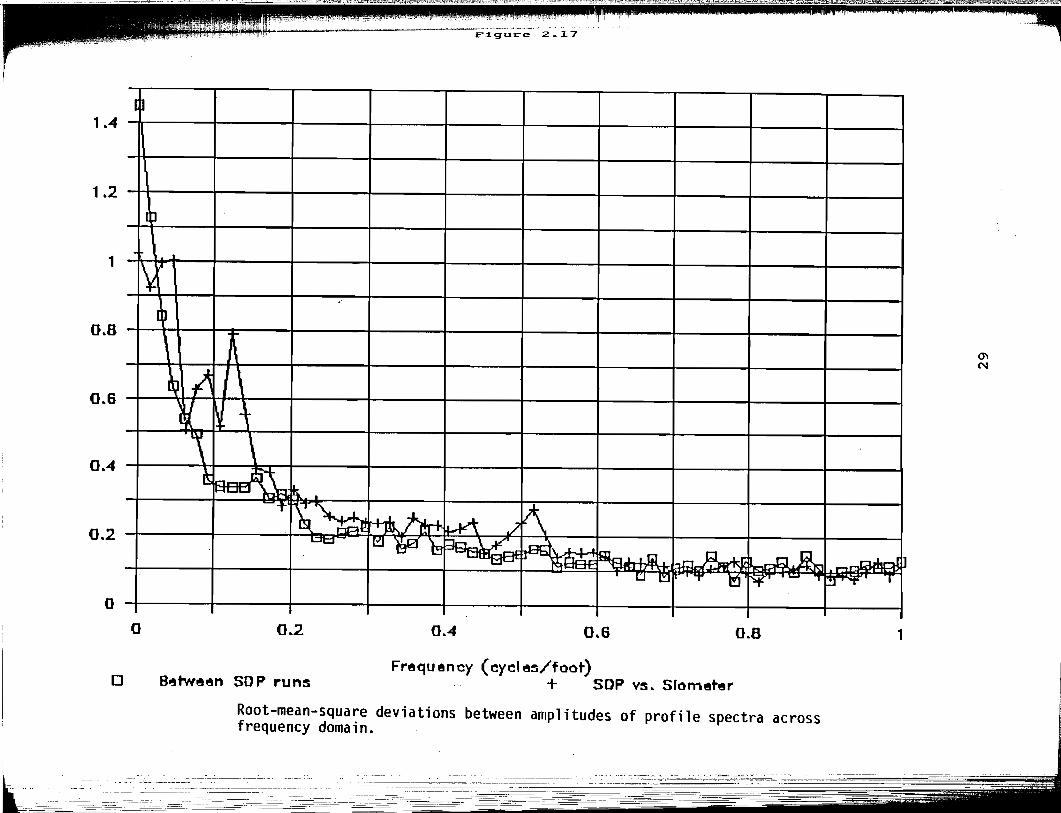
Figure 2.16 shows the correlation coefficients across the frequency domain, between PSO's from repeat SOP runs, and between PSO's from corresponding Siometer and SOP runs. Figure 2.17 shows the RMSO's. It is generally observed that the Siometer power spectra compared favorably with the SOP power spectra. However, at a frequency of 0.125 cycles/foot (about 3.7 hertz at 20 milesfhour), the agreement is not as good as compared with the other frequencies. At 0.125 cycles/foot, the correlation coefficient between Siometer and Profilometer PSO's drops to about 0.65 as observed from Figure 2.17. This result suggests that a fundamental response frequency of the vehicle has not been completely removed and that a need exists for fine-tuning the procedure to parameterize the statistical model of the vehicle so that better agreement between the power spectra of Siometer and SOP profile elevations may be achieved within the entire frequency range.
Thus there is a good agreement between the two profile measuring techniques for the longer wavelengths, but the higher frequencies, beginning with about eight feet wavelength and shorter (about 3.7 hertz at 20 milesfhour), the Siometer process does not have the resolution typical of the laser based SOP. This differences can be contributed to either the modeling procedure, or the inability of using only an accelerometer to obtain such wavelengths. Much of the resolution is lost because of the tire footprint and the attempt to model the overall right and left vehicle characteristics by a linear difference model.
27

""'" c • ~ --• 0 0
c ~ ""'" 0-.,.
f L 0 0
1
0.8
0.6
0.4
0.2
0
0
Figure 2.16
0 0.2 0.4 0.6
Frequency (cycles/foot) B~tw~en SOP runs + SOP vs. srometer
0.8 1
Q) N
Correlation coefficients between roughness power spectral densities across ~
15 frequency d~ain. ..
I 1.4
1.2 ]
1
0.8
0.6
0.4
0.2
0
0
0
--,-
I
\ ~ \
~li \ ~ I~ 1 \ ' \
k ~~~ rt.. '"t'
~~~ ~h-+ l.¥'\ t\ ./ ~ [::j~~ t::h _\ ~
~ -u::J. Q .. LI': .t:l~ ~ !tiki.L..Ltil, t.;.l-
u ~ T 1!1 ¥' ....
0.2 0.4 0.6 0.8
Frequency (eyele!'>/foot) Bl!ltwl!len SOP run!'> + SOP V!'>. Srometer
Root-mean-square deviations between amplitudes of profile spectra across frequency domain.
r:J.I.....J 1
1!1~ I
1
0'1 N

CHAPTER 3
SUMMARY AND CONCLUSIONS
From the results of the preceding chapter it appears that the self-calibrating process does a good job of measuring the longer profile wavelengths (about eight feet and greater). The shorter wavelengths are somewhat attenuated. When the Siometer is located in a standard vehicle and measurements taken at highway speeds with a single accelerometer, the method will typically yield smoother PSI measurements when these profiles are run through the PSI program used by the State (Vertac),because of its inability to measure the smaller wavelengths as accurately. This difference is one of the primary factors adjusted when correlating PSI and WSV values (Ref. 3).
Although not discussed in the previous chapter, profile measurements were also made before and after an overlay project. The results of the SOP runs are depicted in Figure 3.1. Upon examining the two profiles, it is difficult to discern much information from the two profiles, except that the 'after' run does not have some of the peaks as that of the 'before'. The SI computations were more revealing, showing an improvement from 3.1 to 4.2 for the section shown. The point is, however, it is unlikely that the Siometer could be used for any type of improvement measurements, particularly at highway speeds, in its current configuration, except to note such statistics as a change in SI. That is, using profile for determining the necessary amount of fill, etc., is questionable. Even for the SOP to be used for such detail profile measurements, a number of runs for adjacent wheel paths would probably be necessary.
From the above discussion it is concluded that the profile estimates from the Siometer for the near future should be used for PSI (or IRI) measurements for which the current system is designed or for measuring longer wavelengths which are closely correlated to the SOP. However, from the close results noted when installing the Siometer on the SOP as discussed in the preceding chapter, it might be possible to use the self-calibrating process of the Siometer on a small light weight vehicle or trailer towed by such a vehicle at a much slower speed to more accurately obtain the short wavelength information. Additionally, since the R680 system has recently been upgraded to measure profile using the South Dakota profile measuring process, it could also be investigated as an inexpensive method for obtaining more accurate profile measurements. Either the SOP or the Siometer in one of the two modes, might provide profile suitable for
30

!j
' i I , '
t,;;l ,... Ill t!'t'
~ ~ (';!
"'to~!! ,!:!:" .~ ~
t:jlll ""~) l'll:t
(',, ~r;·
,.... :$
CD • Ul ..,
I ,.... . (.1'1 = 5:1 •
I ,....
~
I Cl • (.1'1 Cl
lll ........ :z 111!:1-::t~lll=~:r~
Cl Cl . • . ~
(.1'1
Cl i =~-------;r-----~~~~---+--------+--------T------~
=
C!
.:~~-
~
I
I
~l en en 0 ..... "0 0 a
ttl C1' ttl ..,
... 1 c.~ t!:l --
)~ .....r.::. """~........:-·
.. -- ........... ~.s;· .... - -~
£' -----N
~ -. --
N . U'1 _L. __ , __ _L~---_J_-----l-------~-------'--··----
;-,
31
"'d t"' 0 iool
0 ~
t-Il ::!:: ~
~i!:i• =:JI 0 l'!'j ~
r"l tfj

construction control if a number of profile runs could be made at (for the Siometer) a low measurement speed, eg., 5 MPH. The use of the Self calibrating process with the accelerometer located on the axle of a trailer with small diameter wheels could possibly detect wavelengths in the one foot or less range. Slow speeds tor the South Dakota process would allow more than one distance measurement per foot, which is typical of the South Dakota process for higher speed measurements.
Thus in summary, it is recommended that the current use of the Siometer for SI be continued, and its use for profile estimates in various vehicles be limited in its current configuration. Since the Siometer can be slightly modified to also measure profile using an acoustic sensor and accelerometer in the south Dakota mode, it is recommended that this mode be used and evaluated. It is further recommended that the use of the Siometer on a trailer or small light weight vehicle be investigated for comparing the self-calibrating method and South Dakota method with the SOP and/or rod and level measurements for possible construction control uses.
32

REFERENCES
1. Walker, R. s., "A Self-Calibrating Roughness Measuring Process," Research Report 279-1, Texas Department of Highways and Public Transportation, Austin, Texas August 1982.
2. Hankins, Kenneth D. "The Siometer," Texas Department of Highways and Public Transportation, Research Report 187-ll, January 1985.
3. Walker, R. s., and Luat, Tan Phung, "The Walker Roughness Device for Roughness Measurements," Research Report 479-1F, The University of Texas at Arlington
4. Huft, David L., "Description and Evaluation of the South Dakota Road Profiler", U. s. Department of Transportation Federal Highway Administration, FHWA-DP-89-072-002, November 1989.
5. Sayers, M. w., Gillespie, T. D., and Queiroz, c. A. v., "The International Road Roughness Experiment - Establishing Correlation and a Calibration Standard for Measurements, " World Bank Technical Paper Number 45, World Bank, Washington, D. c., 1986.
6. Spangler, E. B., and Kelly, W. J., "GMR Road Profilometer- A Method for Measuring Road Profiles," Research Publication GMR-452, Engineering Mechanics Department, General Motors Corporation, December 1964.
7. Walker, Rogers., and Schuchman, John Stephen. "Upgrade of 690D Surface Dynamics Profilometer for Non-Contact Measurements," Texas Department of Highways and Public Transportation, Research Report 494-1F, January 1987.
8. Fernando, G. Emmanuel, Roger S. Walker, and Robert L. Lytton, "Evaluation Of The Siometer As A Device For Measurement Of Pavement Profiles., Presented at the 69th Annual Meeting Transportation Research Board, Washington, D.C., January 1990.
9. "Programs for Digital Signal Processing" IEEE Press, 1979, Periodogram Method for Power Spectrum Estimates, L. R. Rabiner, R.W. Schafer, and D. Dlugos,; A Coherence and Cross Spectral Estimation Program, G. Clifford Carter and James F. Ferrie.
33

r • I
)0-
L. mt .ng
s, R. ISS
F.
APPENDIX
PROFILE ANALYZER PROGRAM DESCRIPTION
34

OUTLINE OF THE PROFILE ANALYZER
Part I Introduction and Overview
Part II Structrure Design of Profile Analyzer
Part III : Implementation of Profile Analyzer
1) Flow Chart of Main Program
2) Flow Chart of Lineup and Coherence Procedure
3) Flow Chart of Power Spectrum Procedure
Part IV Simple User Menu
35

Ill" I
------------·············-- ---
Part 1 : Introduction and Overview
In order to compare profile between different measuring
instruments, a set of spectral analysis routines are
developed.
The routines were written to provide the user with both
the analysis results as well as a graphical display.
The Microsoft Quick C language was used for implementing
the various analytical methods.
36

Part II : Theoretical Basis of Profile Analysis
Since profile measurements from differnt instruments
often start at different points a line up method is needed,
Once lined up, more accurate Power spectrum and MSC can be
computed. These basic analysis routines are offered:
1) Cross Correlation (used for Line Up) Estimation
2) Power Spectrum Analysis
3) Magnitude Squared Coherence (MSC) Estimation
37

I i
Part II
File Selection
Structure Design of Profile Analyzer
Profile Analyzer
I I I I I I
Profile Plotting
L ne Up
I I I I I I
Plot Window
Lag Window
38
I I I I I I
Plot
I I I I I I
Power Spectrum
I I I I I I
Data Output
I I I I I I
Coherence Estimation
I I I I I I
I I
Coh-data
I I I I I I
Exit
Windov.· Window Coh-plot Windov.'
Power Spectrum Window

Part III Implementation of Profile Analyzer
1. Main program
Select right ot left
Plotting
Lineup Two signals
Compute Power spectrum
Compute Coherence
Start
Display main menu
Use letter, up or down array to make selection
Select file ?
Plot profile ?
Line up ?
Power spectrum ?
coherence estimate ?
39

2. Lineup and Coherence procedure
Start
Input Parameters
Read a segment
NNN Number of data pts per segment
NDSJP Number of Disj (Nonoverlapping) segments
ISR Sampling Rate SFX,SFY Data scale
factor
of 2-column data from two signals file
Multiply data segment by cosine window
Compute NNN point FFT
Estimate spectral density matrix
Update running sum of estimate
More data
40

Compute
Cross correlation or
Magnitude squared coherence
cross correlation
Graph plotting
Stop
41
Compute MSC

3. Power Spectrum Procedure
Start
Input Parameters
Estimate mean ane variance
Generate and Store window
M L !WIN FS
Obtain 2 segments of data
Remove mean and Apply window
Compute periodograms of 2 segments and accumulate
All data done?
42
FFT length Window length Type of windov,· Sampling rate

Normalize
Compute log power spectrum
Two files done ?
Graph plotting
stop
43

Part IV : Simple User menu
Several points need to be known before this program
starts running.
1) When typing in the file name in the parameter windows,
make sure the string of file name doesn't exceed the
window bounds. Otherwise the program will probably
not run correctly.
2) Make sure that all the input files contain two columns
of data, that is, right and left wheel data. When the
files are opened and the data is input from the files
from option 2 to 5 of main menu, the average of left
and right wheel data is always calculated. For option
1, File Selection, we simply ignore the case of
average wheel data selection.
3) This program is designed to always work with two
files, typically for comparison. If analysis is to be
with only one, the same file can be selected twice. A
maximum of only 3000 sets (right and left) of data can
processed for each file. If the input file contains
more than 3000 sets of data, those data after 3000
sets are ignored.
44

4) The graphic plot of this program has been successfully
displayed on the monitors with the following graphic
cards:
VGA Graphic Card, 640 * 480, BW
VGA Graphic Card, 640 * 480, 16 color
EGA Graphic Card, 640 * 350, BW
EGA Graphic Card, 640 * 350, 4 or 16 color
CGA Graphic Card, 640 * 200, BW
CGA Graphic Card, 640 * 200, 16 color
Plasma Display, 640 * 200, BW
And the graphic plots by pressing PRINTSCREEN has also
been successfully sent to the:
Epson LQ series
Epson FX series
Texas Instruments MODEL850 printer
45

When this program starts running, the screen will look
like Fig 1. There are six options in the main menu.
1. File Selection ---- Select right or left wheel data
There are two columns of data in input file. Left
column means right wheel data, and right column means
left wheel data.
File parameters window would be shown on the right
side of main menu screen.
File parameters
File 1 : (1)RT (2)LT Select one (1-2) File saved as :
File 2 (1)RT (2)LT Select one (1-2) File saved as :
46

2. Profile Plotting ---- Plot profile.
Profile parameters window would be shown on the
right side of main menu screen.
I I I I
Profile parameters
: File 1 I I I I I I I I I I I I I I
' I I I I
' I I
File 2 ' I I I I I I I I I
' I I I I I I I I I I I I I I I I
Four choices on this profile graph :
p PRIKTSCREEN, Print the graphchart on screen.
Retype any key would abort the print
s SELECTRAKGE, Select range of this graph and
plot it. Select range ~indow would be
shown on the top left part of profile
plot screen.
No. of points altogether *** No. of points selected Start pt of signal 1 Start pt of signal 2 :
47
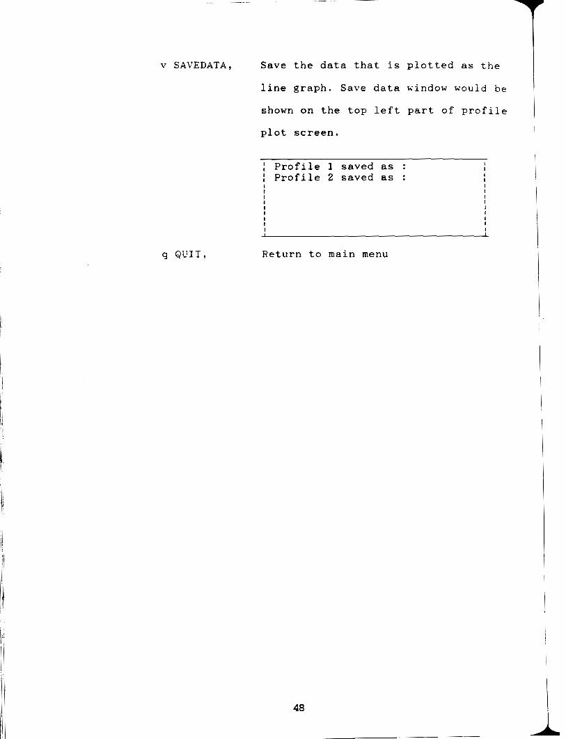
v SAVEDATA, Save the data that is plotted as the
line graph. Save data ~indow would be
shown on the top left part of profile
plot screen.
Profile 1 saved as Profile 2 saved as
g QUIT, Return to main menu
48 l

3. Line Up---- Lineup two signals.
Lineup parameters window would be shown on the
right side of main menu screen.
I I I
Lineup parameters I I I I I I
1
: File 1 I I I I I I I I I I I I I I I I I
File 2
~ I I I I I I I I I I I I I I I I
The lag number in which maximum cross correlation
corresponds is shown on the left bottom corner in
There are three choices on this graph :
p PRINTSCREEN, Print the graph on screen.
Retype any key would abort this
f PROFILE, See the profile of two signals after
being lined up.
q QUIT, Return to main menu
There are four choices:
p PRINTSCREEN, Print the graph on screen
s SAVEDATA, Save the data that is plotted
as the line graph. Save data window
is the same as the one in option 2
c CROSSCORRELATION, See plot of cross correlation
q QUIT, Back to main menu
49

4. Power Spectrum---- Compute the power spectrum of
two signals.
Power spectrum parameters window would be shown on
the right side of main menu screen.
:Power I
spectrum parameters I I I I I I I I I I I I I I I l l I I I I I I I I I I I I I I I
File 1 : File 2 FFT length Window length \>.' indow Type :
(1=RECT 2=HAMMING) Sampling Rate :
(Cycle per Foot)
I I I I I I I I I I I I I I I I I I I I I I I I I I I I I I I I I I I
FFT length must be a power of 2
2 <= FFT length <= 1024
Window length <= FFT length
Fig 5 show all the important statistical values
like mean value, variance value, max DB, min DB and
DB variation.
There are three choices:
p PRINTSCREEN, Print the graph on screen.
Retype any key would abort this
d PRINTDATA, Print power spectrum data of two
signals
Return to main menu
50
I I
l

5. Coherence Estimation---- Estimate coherence of
two signals
Coherence parameters window would be shown on the
right side of main menu screen.
Coherence parameters
File 1 : File 2 : FFT length Disj Segs Number Sampling Rate : Scale Factor 1 Scale Factor 2 :
~ote: Sampling points = FFT length * Disj Segs Number
The total sampling points are not allo~ed to be
over the points inputed , or error messages would
be given. Then type in all the parameters again.
There are fo.ur choices on data window :
PgUp, See the data of last screen
PgDn, See the data of next screen
p PLOTTING, See the plot of MSC data
q QUIT, Return to main menu
51
~ i

There are four choices on Fig 8 :
p PRINTSCREEN, Print the graph on screen.
Retype any key would abort this
d PRINTDATA, Print the data as plotted on this
graph
w DATAWINDOW, See the data window
q QUIT, Return to main menu
6. Exit ---- Exit this program.
52
---------------

I I I I I I I I I I I I I I I I I I I I I I I I I I I I I I I I I I I
PROFILE ANALYZER
File Selection Profile Plotting Line Up Power Spectrum Coherence Estimation Exit
Use letter, up or down arrow to make your selection
* Select right or left wheel data *
Fig 1
53
I I I I I I I I I I I I I I I I I I I I I I I I I I I I I I I I I I I