Use of PITA for Estimating Key Reservoir … PAPER 2006-172 Use of PITA for Estimating Key Reservoir Parameters N.M.A. RAHMAN, M. POOLADI-DARVISH, M.S. SANTO, L. MATTAR Fekete Associates

1

PAPER 2006-172

Use of PITA for Estimating Key Reservoir Parameters

N.M.A. RAHMAN, M. POOLADI-DARVISH, M.S. SANTO, L. MATTAR Fekete Associates Inc.

This paper is to be presented at the Petroleum Society�s 7th Canadian International Petroleum Conference (57th Annual Technical Meeting), Calgary, Alberta, Canada, June 13 � 15, 2006. Discussion of this paper is invited and may be presented at the meeting if filed in writing with the technical program chairman prior to the conclusion of the meeting. This paper and any discussion filed will be considered for publication in Petroleum Society journals. Publication rights are reserved. This is a pre-print and subject to correction.

Abstract Well testing is sometimes reduced to perforating the well,

capturing the pressure data and analyzing the data. The primary objective of a Perforation Inflow Test Analysis (PITA) is to estimate the initial reservoir pressure, permeability and skin, for evaluating future development strategy. However, special analytical procedures are required for analyzing the data, because these perforation inflow tests are considerably shorter than conventional well tests, and there is no recorded production.

In this study, a systematic analytical procedure for estimating meaningful reservoir parameters from perforation inflow tests will be presented. Two major aspects of data interpretation will be discussed � Diagnostic Analysis and Modeling. A straight-line approach is taken to analyze the early-time and late-time data. A special diagnostic technique is required for detecting and estimating positive or negative skins. A distinctive feature of PITA, is that it does not require calculation of the inflow rates. Note that the same approach can be applied in over-balanced situations, when there is fluid efflux, rather than fluid influx.

When employing straight-line analysis techniques, acceptable estimates of initial reservoir pressure, permeability and skin are only obtained if the test duration is sufficient to

achieve radial flow. This is usually not a problem in high permeability reservoirs. However, in low permeability reservoirs, the test duration required to reach radial flow can be prohibitively long. In these cases, the test is often terminated during the transition from wellbore storage to radial flow. Consequently, acceptable estimates of initial reservoir pressure, permeability and skin can only be obtained by extending the analysis into modeling. Field examples will be presented to highlight the methodology. A rigorous technique for estimating the radius of investigation during the test will be discussed. It will be shown that in the presence of measurement errors, radius of investigation will grow to a maximum value. Running the tests for anytime longer will be dominated by the noise.

Introduction Well tests have been the primary and most reliable means of

characterizing reservoirs for decades. However, there has been a growing trend over the last several years to search for alternatives that could yield the desired information in less time, in a more environmentally-friendly manner, and at a cheaper cost than conventional well tests. The desired change has inevitably been towards tests of shorter duration.1-4 Although it is accepted that results from short tests with small radii of

PETROLEUM SOCIETY CANADIAN INSTITUTE OF MINING, METALLURGY & PETROLEUM

2

LT

wi

m

ppCkh

2

)( )10842.1)(24( 03

investigation may not be as reliable as those from conventional well tests, it is reasonable to accept that they could be of value in assisting with strategic decisions about field development, when an increased margin of error can be tolerated.

In offshore wells, in addition to the potentially exorbitant cost of testing (several millions of dollars), the drive towards green (shorter) tests is fuelled by environmental considerations, such as requirements for restricted flaring of hydrocarbons. In Alberta and elsewhere in North America, the driving force towards inexpensive tests is the marginal economics of low deliverability wells. Either way, there is an increasing trend towards these green tests to replace conventional well tests. One such green test consists of simply allowing the well to flow into the closed wellbore after perforating, when there is an under-balanced wellbore condition. As the fluid from the reservoir enters the wellbore (with a fixed volume), the wellbore pressure builds up. The pressure data is collected either downhole or at the wellhead for a period of hours or days, depending on the reservoir�s flow potential. These tests have been variously called: Slug test, Surge Test, Perforation Inflow Diagnostic (PID), or Closed Chamber Test.

The basis of Perforation Inflow Test Analysis (PITA) is the slug-test model originally proposed by Ramey and co-workers5,

6 in the seventies. In related works of Soliman1 and Ayoub et al.2, it is shown that the late-time shut-in data is not a function of the flow rate and its variation with time, but a function of total volume of fluid influx. While most of the previous solutions presented for tests with a short inflow period concentrate on the late-time analysis for determination of permeability and initial reservoir pressure, PITA is extended to include early-time analysis and used for determination of skin. This additional information is very useful for making decisions on the need for stimulation in cases where inflow rate is poor because of large skin, rather than low permeability.

Two previous publications7, 8 have provided a systematic procedure for analysis of data from perforation inflow tests. However, these presentations have not been able to calculate the zero or negative skins from PITA. Since then, we have considered the possibility of the test well having no skin or an improved zone (negative skin) around the wellbore. Therefore, in this study, we are going to present diagnosis and quantification of positive, zero and negative skins, using PITA. We are also presenting how the estimates of initial reservoir pressure, permeability and skin can be improved through analytical modeling of the entire test data from perforation tests. We also present new field examples to illustrate advantages of PITA. An investigative discussion on the radii of investigation during perforation tests is also included. On a related note, the methodology of PITA can be extended to over-balanced situations, when there is fluid efflux, rather than fluid influx. However, this extension needs an appropriate modification of the wellbore storage calculations.

Working Equations and Analysis Procedure

Details of the mathematical development of PITA have been presented in Reference 8. The early-time data is used to estimate skin, and the late-time data to estimate initial pressure and permeability. In gas wells, the pressure data is usually measured at the wellhead, and is converted to the bottom-hole condition. This conversion is primarily due to hydrostatic head, because the influx rate into the wellbore diminishes very rapidly, and frictional losses are not significant. Moreover, the

analysis of gas well data requires the conversion of data � pressure to pseudo-pressure, and time to pseudo-time (viscosity and total compressibility are evaluated at well pressure). The fluid influx rate into the well is not measured, nor is it necessary for the analysis.

The working equations in practical metric units for liquid (single-phase oil or water) and gas cases, including the possibilities of the positive, zero and negative skin factor, are presented below:

Case I: Liquid Influx Here we are considering a single-phase liquid (oil or water) flow situation in the presence of a compressible formation.

a. Analysis of Late-Time Data

Analysis Equation:

tkh

ppCpp wi

iw

2

)( )10842.1)(24( 03

��....�..(1)

Plotting Functions: pw vs. 1/t. Analysis Line: Draw a straight line through the late-data points.

Calculation Procedure: i. Determine the intercept at 1/t = 0, which is indeed pi. ii. Estimate the slope of the late-time analysis line, mLT

(absolute value), and calculate kh as:

��......�...(2)

b. Analysis of Early-Time Data

1. For skin factor, s > 0: Analysis Equation:

sC

tppkhpp wi

ww )10842.1)(24(

)( 3

00

��.....��..(3)

Plotting Functions: pw vs. t. Analysis Line: Draw a straight line through the early-data points, anchoring on pw0 (if it is reliable).

Calculation Procedure: Estimate the slope of the early-time analysis line, mET, and use the pi and kh values from the late-time analysis (done earlier) to compute s as:

ET

wi

mC

ppkhs

)10842.1)(24(

)( 3

0

��.....��..(4)

2. For skin factor, s ≤ 0: Analysis Equation:

3

2a23

2

)10)(1.842(0.159)(24

w

t rC

tchk

wat r

k

tc

C

hk

106.3

)101.842( )24(

263

0 )10842.1( )24( )2(

3

0

0

C

thk

pp

pp

wi

ww

�....(5)

As illustrated above, for estimating s ≤ 0, our target is to estimate the effective wellbore radius, rwa, from Equation 5. The details of the derivation of Equation 5 are presented in the Appendix. Plotting Functions: pw vs. t. Analysis Line: Draw a straight line through the early-data points, anchoring on pw0 (if it is reliable). Calculation Procedure: i. Select a data point (t, pw) on the early-time analysis

line, and set up the quadratic equation in rwa (Equation 5), using the pi and kh values from the late-time analysis (done earlier) and the other input parameters.

ii. Solve the quadratic equation (Equation 5) for two values of rwa. Normally, it is trivial to figure out which of these two values represents the system in question, as the rejected value of rwa is an unrealistically huge number.

iii. Use the selected value of rwa to calculate s as:

w

wa

r

rs ln ��...(6)

Note that for rwa = rw, s = 0, and for rwa > rw, s < 0.

Remarks: The wellbore storage constant C in Equations 1

through 5 for liquid influx can be estimated from one of the following equations:

1. For Changing Liquid Level:

g

VC u

)000,1(

��.�..��(7)

2. For a Closed Chamber Filled with Compressible Liquid:

ww cVC ��..��(8)

Note that the cushion pressure, pw0, must be known or estimated prior to performing any of the late-time or early-time data analyses.

Case II: Gas Influx We are considering a single-phase gas flow situation in the presence of residual fluid saturation and a compressible formation. Here gas is the only mobile phase, and the water phase is immobile. To correct for the variations of the viscosity and compressibility of gas with pressure, we need to use

pseudo-pressure and pseudo-time, replacing pressure and time, respectively. These pseudo-variables can be defined as9 -

Pseudo-pressure:

p

Z

pdpp

0 2)(

��..�� (9)

Pseudo-time:

t

wtwa

pcp

tdtt

0 )( )()(

��..��.��.............(10)

a. Analysis of Late-Time Data

Analysis Equation:

a

wiwiw tkh

V

2

)( )10842.1)(24( 03

��..�..(11)

Plotting Functions: w vs. 1/ta. Analysis Line: Draw a straight line through the late-data points.

Calculation Procedure: i. Determine the intercept at 1/ta = 0, which is i. Then,

convert i to pi. ii. Estimate the slope of the late-time analysis line, mLT

(absolute value), and calculate kh as:

.��.......�...(12)

b. Analysis of Early-Time Data

1. For skin factor, s > 0: Analysis of Equation:

sV

tkh

w

awiww

)10842.1)(24(

)( 3

00

��...��(13)

Plotting Functions: w vs. ta. Analysis Line: Draw a straight line through the early-data points, anchoring on w0 (if it is reliable).

Calculation Procedure: Estimate the slope of the early-time analysis line, mET, and use the i and kh values from the late-time analysis (done earlier) to compute s as:

ETw

wi

mV

khs

)10842.1)(24(

)( 3

0

��.....��..(14)

2. For skin factor, s ≤ 0:

LT

wiw

m

Vkh

2

)( )10842.1)(24( 03

4

Analysis Equation:

2a2

w3

2

)101.842 ( (24) (0.159)

w

a rV

thk

waa

w

rk

t

V

hk

106.3

)101.842( )24(

233

0 )101.842( )24( )2(

3

0

0

w

a

wi

ww

V

thk

.�..(15)

For estimating s ≤ 0, our target is to calculate the effective wellbore radius, rwa, from Equation 15. The details of the derivation of this equation are presented in the Appendix. Plotting Functions: w vs. ta. Analysis Line: Draw a straight line through the early-data points, anchoring on w0 (if it is reliable). Calculation Procedure: i. Select a data point (ta, w) on the early-time analysis

line, and set up the quadratic equation in rwa (Equation 15), using the i and kh values from the late-time analysis (done earlier) and the other input parameters.

ii. Solve the quadratic equation (Equation 15) for two values of rwa. Normally, it is trivial to figure out which of these two values represents the system in question, as the rejected value of rwa is an unrealistically huge number.

iii. Use the selected value of rwa to calculate s as:

w

wa

r

rs ln ��.....(16)

Note that for rwa = rw, s = 0, and for rwa > rw, s < 0.

Remarks: Observe that the cushion pseudo-pressure, w0,

must be known prior to performing any of the late-time or early-time data analyses. This value can be calculated from the known or estimated cushion pressure, pw0.

Influx Rate Calculations One significant advantage of PITA is that the analyst does

not need to calculate the influx rates as part of the analysis of the data. Often, with a set of noisy pressure data, the calculated rates become noisier. However, the influx rates can be calculated for any other diagnostic purposes by using the material balance principles as shown below:

Liquid Rate

1. For Changing Liquid Level:

)()000,1)(24(

td

dp

gB

V q wu

l

��.........��(17)

2. For a Closed Chamber Filled with Compressible Liquid:

)()24(

td

dp

B

c V q www

l ��..��.��(18)

Gas Rate

)()000,1(

)24(

td

dp

B

c V q w

g

gwg ��.��......(19)

Identification of Flow Regimes It is very obvious that the data for PITA is significantly

influenced by wellbore storage. It is also evident that the data is also directly influenced by the flow capacity (kh) and the skin. Therefore, one needs to distinguish the part of the data dominated by wellbore storage (afterflow effects) from the part of data that is dominated by reservoir characteristics (reservoir pressure and permeability). As shown in Equations 3 through 5, and 13 through 15, the early-time data contains information about the skin, because of significant fluid influx rates (which are affected by the skin value). Also, Equations 1, 2, 11 and 12 demonstrate that the late-time data can be exploited to estimate reservoir pressure and flow capacity (or permeability). Thus, proper identification of these flow regimes is important in order to choose appropriate data ranges from a perforation inflow test for appropriate analyses.

From the authors� experience, it has been observed that the measured pressure in a set of data must contain at least some portion of the reservoir-dominated flow in order for the estimated reservoir pressure, permeability and skin to be representative of the reservoir. Alternatively speaking, the test period must be long enough to see the reservoir-dominated flow at late times. A special kind of derivative, PITA derivative (PDER), is used to confirm if the data has seen the reservoir-dominated flow. Cinco-Ley et al.10 originally introduced this derivative, which can be defined as:

Liquid Influx

td

dptPDER w

2)( ��...��.(20)

Gas Influx

a

wa td

dtPDER

2)( ��.��...��.(21)

This approach is similar to the traditional well-test

interpretation, where a derivative plot is used to differentiate the wellbore flow regime from the infinite-acting radial flow regime. However, the PDER behaves in a slightly different way from the traditional well-test derivative. From our experience, we have observed that the slope of the early-time data (wellbore storage), when plotted with time (or pseudo-time) in log-log scales, can be influenced by the skin. If the well has a positive skin, it will manifest as a slope of 2, and if it has a zero or negative skin, the early-time data will yield a slope of about 1.75 (cf. well-test derivative has a slope of 1). With real field data, it is not easy to distinguish between slopes of 1.75 and 2. The late-time data (reservoir-dominated flow) has a slope of 0 (flat line � the same as the well-test derivative).

Thus, once the PDER has been plotted with time (or pseudo-time) in log-log scales, it is easy to recognize whether or

5

not reservoir-dominated flow exists. If it does, reasonable values of initial reservoir pressure, permeability and skin can be determined. At least some of the late-time data should fall on the flat part of the derivative in order to get a reliable analysis. If this data exists, then skin can be calculated from the early-time data. If there is no reservoir-dominated flow in the perforation inflow test data, then a unique interpretation of the given data by using PITA is not possible.

Interpretation of Test Data In traditional well test interpretation, we start analyzing the

data from early time to late time. In PITA, we start with the late-time data first, to obtain reservoir pressure and permeability. After this, we analyze the early-time data to obtain skin. Even though a complete analysis can be obtained from the derivative plot alone, it is useful to generate specialized plots to confirm the analysis. As presented earlier, the working equations for liquid and gas influxes are slightly different. For liquid influx, the data is analyzed in terms of pressure and time. For gas influx, the data is analyzed in terms of pseudo-pressure and pseudo-time. In liquid influx, we need to specify the wellbore storage constant (C) due to a changing (rising) liquid level in the wellbore, which is a function of wellbore capacity (Vu) and liquid density, or due to the wellbore volume (closed chamber volume, Vw), which is completely filled with a compressible liquid. In gas influx, we need to specify the wellbore or chamber volume (Vw). As shown earlier, wellbore volume or wellbore capacity needs to be known a priori for estimating the reservoir parameters. There can be occasions when these values may not be known with reasonable accuracy. In such situations, an over-estimated wellbore volume or wellbore capacity will lead to an over-estimation of permeability by the same proportion (see Equations 1, 11 and 12). Similarly, an under-estimated wellbore volume will lead to an under-estimated permeability. However, the estimates of the initial reservoir pressure appear unaffected, when the wellbore volume or wellbore capacity is in error. Also, the estimates of skin (especially, s > 0) are not affected, as the permeability compensates for any error in estimated wellbore volume or wellbore capacity (see Equations 4 and 14). Note, that for liquid or gas efflux (when there is an over-balanced wellbore condition), a pressure falloff will occur, and can be analyzed in the same manner as for liquid or gas influx, by adjusting the storage (C) calculations appropriately.

An important question one may face, when observing a slow rate of pressure buildup in the wellbore, is whether the poor performance is because of high skin or low permeability. While the latter cause may lead to an abandonment of the well, the former may be resolved by stimulation. The greatest advantage of PITA is to help separate skin from permeability. Once reasonable estimates of initial reservoir pressure, permeability (or flow capacity) and skin are established, the next logical step is to generate synthetic pressures to match the test pressures, using an analytical solution.8 This step helps refine the reservoir parameters already estimated from analysis and will be highlighted while presenting the field examples.

Field Examples In this section, we are presenting three field examples (two

gas wells and one water well), which will illustrate some

practical aspects of analyzing some real data with the proposed methodology.

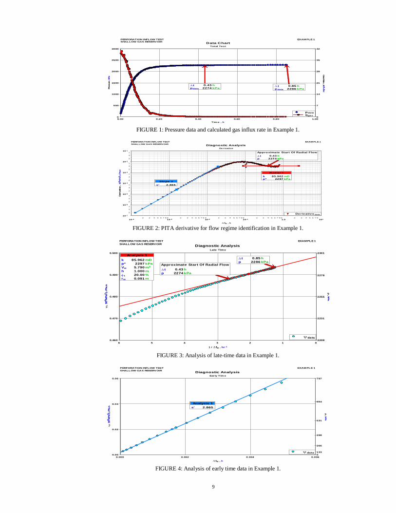
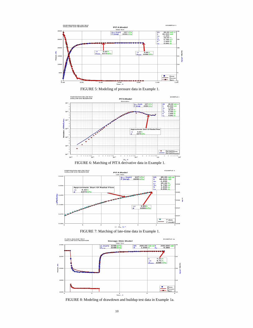
Example 1 represents a perforation inflow test performed on a shallow gas reservoir in the Southern Alberta plains. The well was perforated dry, and pressures were collected at the wellhead. Since the pressure increased very quickly after perforating, the test was terminated after only 0.85 hours. Figure 1 shows the calculated bottom-hole pressures and inflow rates. The PITA derivative (Figure 2) exhibits a slope of �2� in the early time, and a slope of �0� in the late time. The late-time analysis of the PITA derivative and the Cartesian plot of pressure vs. 1/∆ta (Figure 3) yields an estimated permeability of 86 mD and initial reservoir pressure of 2,297 kPaa. The early-time analysis of the PITA derivative and Cartesian plot of pressure vs. ∆ta (Figure 4) yields a skin near zero (+2.9). Extending the analysis into modeling (Figures 5 through 7) confirms the diagnostic analysis, since the reservoir-dominated flow was observed. The radius of investigation of this particular example is discussed in the next section.

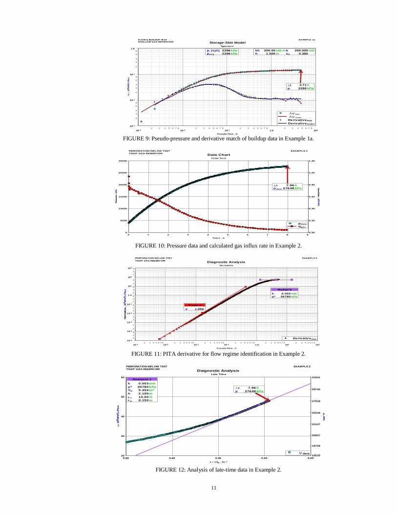
After the perforation inflow test of Example 1, a conventional flow and buildup test was performed on the same well (referred to as Example 1a). The flow period was 2 hours, and the buildup period was 4.7 hours. The pressures were again collected at the wellhead. Figure 8 shows the calculated bottom-hole pressures and measured gas rates. The conventional diagnostic log-log plot (Figure 9) reveals the classic pressure behaviour of wellbore storage and infinite-acting radial flow. The interpretation of this data yields a permeability of 200 mD, skin near zero (+0.4) and pi of 2,296 kPaa. Figures 8 and 9 also present the modeling results. These results show that the earlier perforation test results are consistent with the conventional flow and buildup test results.

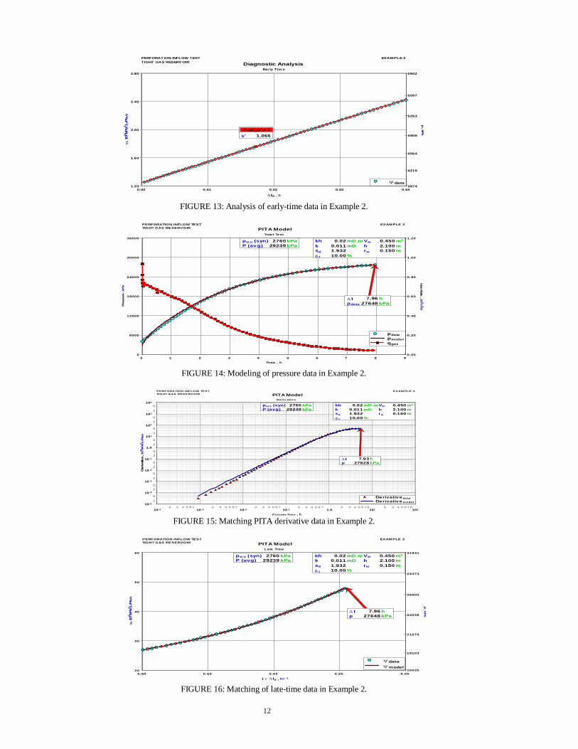
Example 2 corresponds to a perforation inflow test, performed on a tight gas reservoir in the foothills of the Canadian Rockies. Downhole shut-in was utilized to minimize wellbore storage effects, and pressures were therefore measured with a gauge located very close to the perforations. The test was run for 8 hours, while the service rig was shut down for the night. Figure 10 shows the measured bottom-hole pressures and the calculated inflow rates. The PITA derivative (Figure 11) yields a slope of �2� in the early time, and approaches a slope of �0� in the late time. The late-time analysis of the PITA derivative (Figure 11) and the Cartesian plot (Figure 12) estimate pi and k in the order of 31,000 kPaa and 0.003 mD, respectively. The early-time analysis of the PITA derivative (Figure 11) and the Cartesian plot (Figure 13) offer a skin estimate of +1.0. Since reservoir-dominated flow (i.e., slope = �0�) was not developed, the PITA model provides different estimates of initial reservoir pressure, permeability and skin, but they are still of the same magnitude. These results are shown in Figures 14 through 16.

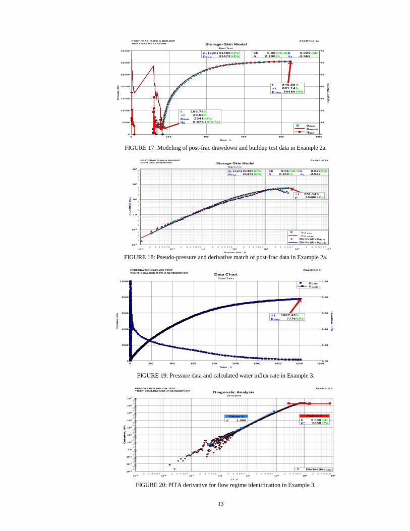
Following the perforation inflow test of Example 2, the same well was hydraulically fractured, and flowed on cleanup for about 30 hours. A memory gauge was then landed near the top of the perforations, and production resumed for another 29 hours. A buildup test was then conducted for a period of one month. The results from this test are presented as Example 2a. The rate history and measured bottom-hole pressures are displayed in Figure 17. The conventional diagnostic log-log plot is displayed in Figure 18. The model results generated from this buildup are shown in Figures 17 and 18. During the flow period, the rate was too low to continuously lift the frac fluid to surface. Consequently, the buildup response was distorted by �phase redistribution� phenomena. Fortunately, the extended buildup duration provided sufficient time for reservoir-

6

dominated flow to develop. The interpretation provided pi and permeability estimates in the order of 31,500 kPaa and 0.03 mD, consistent with the PITA results. The calculated negative skin (-3.6) shows that some improvement was gained from the stimulation.

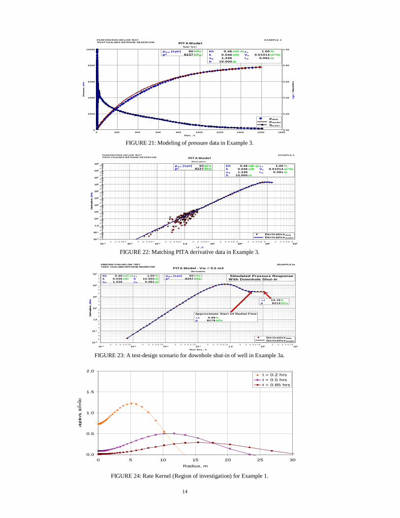
Example 3 depicts a perforation inflow test conducted on a tight (wet) coalbed methane reservoir in Western Canada. The well was perforated dry, and since liquid influx was anticipated, pressures were obtained with a memory gauge set close to the perforations. The pressure buildup was monitored for about 1,600 hours before recovering the memory gauge. Figure 19 shows the measured bottom-hole pressures and calculated water influx rates. The PITA derivative (Figure 20) exhibits a slope of �2� in the early time, and is approaching a slope of �0� in the late time. The late-time analysis of the PITA derivative (Figure 20) estimates permeability and pi in the order of 0.006 mD and 8,900 kPaa, respectively. The early-time analysis of the PITA derivative (Figure 20) yields a skin near zero (+1.1). The PITA model (Figures 21 and 22) yields a skin value consistent with the diagnostic analysis. The estimated pi is within 7% of the diagnostic estimate. However, the model permeability is nine times higher than the diagnostic estimate. This indicates that reservoir-dominated flow was far from being developed within the test period, and that better estimates of pi and permeability are obtained from modeling.

As demonstrated with Example 2, the test duration for tight formations can be reduced significantly when downhole shut-in is utilized. In Example 3 (Figures 19 through 22), downhole shut-in was not utilized, and reservoir-dominated flow was not developed after an extended shut-in period of 1,600 hours. Example 3a (Figure 23) shows the simulated pressure response expected with downhole shut-in (i.e., reduced wellbore volume to 0.5 m3). The PITA derivative indicates that reservoir dominated flow (slope of �0�) would develop within 5 hours of shut-in. Therefore, total test duration of about 12 hours would provide the required results.

Radius of Investigation One drawback of perforation tests is their small radius of

investigation. This is intuitively expected because of the small volume of wellbore into which the reservoir fluids flow. However, a question arises of what the radius of investigation is during a particular test. A related question is whether larger radii of investigation can be achieved by recording the shut-in data for longer times. Previously, Rahman et al.8 argued that in the presence of noise, a perforation inflow analysis can investigate the reservoir only to a particular radius. Shutting the well any longer would detect just the noise. To explain this, the authors used the concept of region of investigation based on the work of Oliver11, and Thompson and Reynolds12. These authors showed that the permeability estimated from a plot of pressure derivative (i.e., derivative of pressure changes with respect to natural log of time) is mostly influenced by a zone in the reservoir, where the rate is changing the fastest with respect to natural log of time. Using this definition, the region of investigation of a conventional drawdown test (at constant rate) is understood in the following way. When a well is produced at a constant rate, there is a region close to the wellbore (Zone I) with a nearly constant reservoir flow rate. Zone I is followed by Zone II, where most of the flow is taken from (by fluid expansion). At the inner radius of this Zone II, flow rate is nearly equal to the flow rate at the wellbore, while at the outer radius of this zone, flow rate is nearly zero. Beyond the outer

radius of Zone II, there is nearly no flow, because the effect of pressure disturbance caused by production at the wellbore has not traveled that far yet. During a drawdown test, the inner and outer radii of Zone II expand with time. References 11 and 12 showed that the pressure derivative reflects the permeability of a zone that closely correlates with Zone II. For liquid flow, this is mathematically shown in Equation 2212.

wrw dr

t

trq

rrkhtd

tpd'

ln

,'

'

1

'

110842.1

ln

3 ��.�(22)

For a homogenous formation, Equation 22 says that the

magnitude of the information arriving from the reservoir (i.e., the pressure derivative function as represented on the left-hand side of Equation 22) is heavily influenced by a function called rate Kernel, ttrq ln/ , (on the right-hand side of Equation 22), which represents that zone of the reservoir where rate is changing the fastest with respect to natural log of time. Graphs of rate Kernel vs. radius demonstrate that region of reservoir which heavily influences the pressure derivative curve (i.e., the region of investigation). Furthermore, the integral under the curve of rate Kernel (when multiplied by 1/r as required by Equation 22) represents the amount of information that is received from the reservoir and is captured in the pressure-derivative function. For a constant rate drawdown, References 11 and 12 showed that during infinite-acting radial flow, the integral remains constant, representing a constant value of the derivative function.

Figure 24 shows a plot of the rate Kernel vs. radius for a perforation inflow test representing Example 1. The following observations can be made:

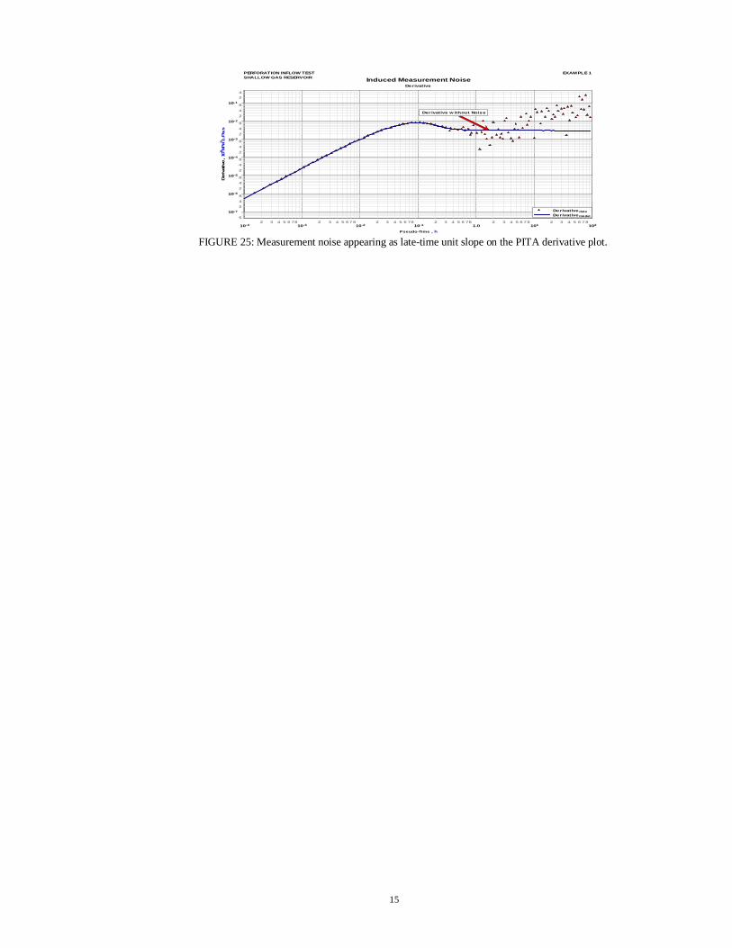
(i) The curves in Figure 24 show the portion of the reservoir that has the largest effect on the pressure derivative, representing the region of investigation. Figure 24 shows that at the end of the test (t = 0.85 hr), the PITA derivative is influenced by a region of about 30 m around the wellbore, with maximum influence coming from the peak of the rate Kernel at about 15 m. We have confirmed that the region of investigation propagates linearly with square-root of time and is a function of square-root of hydraulic diffusivity. This behaviour of radius of investigation of a perforation inflow test is similar to that of a constant-rate production test. (ii) The maximum value of the curves and the integral under the curves of Figure 24 (when multiplied by 1/r as required by Equation 22) are decreasing with time. Therefore, the magnitude of information that is contained in the pressure-derivative values decreases with time. The implication is that, unlike in a constant rate drawdown test, in a perforation inflow test and in the presence of some measurement noise, a time will come when the magnitude of the information being transferred from the reservoir to the wellbore becomes less than that in the noise. Beyond this time, i.e., when the noise-to-signal ratio becomes significant, the pressure derivative plot would be dominated by noise. In Figure 25 (the same as the Example 1 case presented in

Figure 6), the solid line shows the PITA derivative in the absence of any measurement error. The duration of the actual test was just under an hour which allowed detection of the beginning of radial flow as explained previously. The results

7

shown in Figure 25 have been extended to 100 hours to find out whether a larger radius of investigation would have been obtained if the shut-in pressures were measured beyond the actual end of the test. To answer this question, we have generated the PITA derivative of the same example where the pressure data is corrupted by some normal random errors with a mean of zero and a standard deviation of 0.5 kPa. Figure 25 shows that, for some time, the noise does not affect the analysis, such that the PITA derivative displays the wellbore-storage dominated flow, followed by the transition to the reservoir-dominated flow. This latter portion is however short-lived, and is soon masked by the noise.

Figure 25 also shows that, in the presence of noise, the PITA derivative at late times deviates from the flat PITA derivative, and exhibit unit-slope behaviour with significant scatter. The latter is devoid of reservoir information and is a representation of a normal random error with mean of zero, which when logarithmically distributed in time and plotted on a log-log plot of the absolute value of the PITA derivative vs. ∆ta would tend to show as a unit slope. Therefore, in this case, waiting longer than about an hour would not have led to any deeper investigation of the reservoir.

This exercise shows that a small amount of noise after some time could easily mask the reservoir information from a perforation inflow test, whose influx rate is continuously deceasing with time. This time corresponds to the maximum radius of investigation of a perforation inflow test (about 30 m for Example 1 with a random noise of 0.5 kPa). The time interval where useful data could be collected depends on the ratio of the magnitude of information coming from the reservoir and the magnitude of the noise. For a particular reservoir response, the smaller the noise, the longer the duration of useful data. When the main source of noise is from the pressure gauge, use of accurate pressure gauges could allow obtaining larger radii of investigation in perforation inflow tests.

Conclusions 1. Using a systematic and comprehensive method to analyze

data obtained from perforation inflow tests, reasonable estimates of key reservoir properties can be obtained, if the data sees at least some portion of the reservoir-dominated flow. A successful test requires that there is good communication established with the �unaltered reservoir� beyond any damaged zone.

2. Modeling of the entire test data with the analytical

solution helps refine the reservoir parameters already estimated from PITA.

3. Use of downhole shut-in can significantly reduce the test

duration required to observe reservoir-dominated flow in tight formations.

4. A time was identified when the errors in the pressure

measurement (e.g. measurement noise) would mask reservoir information, and would render longer shut-ins unnecessary. This time corresponds to the maximum radius of investigation of a perforation test.

Acknowledgements The authors wish to thank the management of Fekete

Associate Inc. for permission to publish this paper, and Mr. Florin Hategan of Burlington Resources Canada Ltd, for his assistance in collecting field examples.

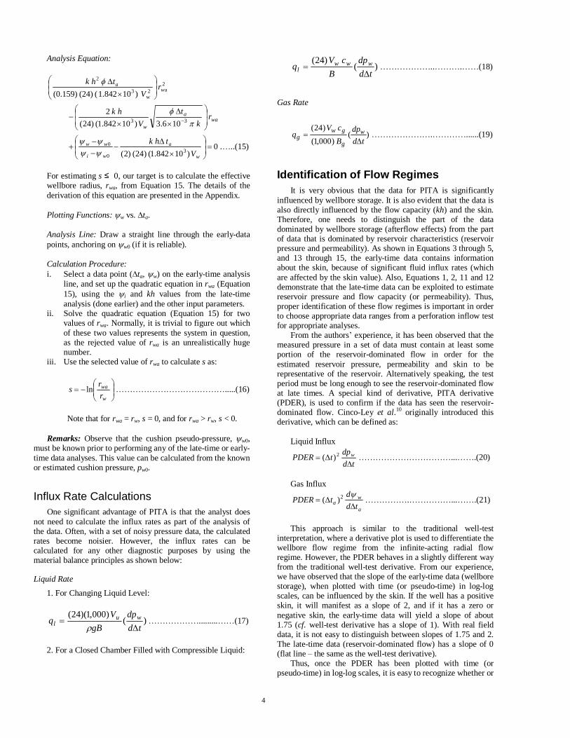
NOMENCLATURE B = Liquid formation volume factor, m3/m3 Bg = Gas formation volume factor, m3/m3 cg = Gas compressibility, kPa-1 ct = Total system compressibility, kPa-1 cw = Liquid compressibility, kPa-1 C = Wellbore storage constant for rising liquid level (oil or water), 1,000Vu / ( g), m3/kPa CD = Dimensionless wellbore storage constant, defined in Equation (A-2) for liquid, and in Equation (A-6) for gas g = Acceleration due to gravity, 9.80665 m/s2 h = Net pay thickness, m k = Permeability, mD mET = Slope of early-time analysis line (s > 0), kPaa/hr mLT = Slope (absolute value) of late-time analysis line, kPaa-hr for liquid, and (kPaa)3-hr/(Pa.s)2 for gas PDER = PITA derivative, defined in Equation 7, kPa-hr (liquid), and in Equation 8, (kPaa)3-hr/(Pa.s)2 (gas) pi = Initial reservoir pressure, kPaa pw = Pressure at wellbore, kPaa pw0 = Initial cushion pressure or wellbore pressure at time t = 0, kPaa qg = Rate of gas influx into wellbore, 103m3/d ql = Rate of liquid influx into wellbore, m3/d rw = Wellbore radius, m rwa = Effective wellbore radius, m s = Skin factor tD = Dimensionless time, defined in Equation (A-3) for liquid, and in Equation (A-7) for gas t = Time since beginning of fluid influx, hr ta = Pseudo-time since beginning of gas influx, hr-kPa/Pa.s Vu = Wellbore volume per unit length (wellbore capacity), m3/m Vw = Wellbore (chamber) volume, m3 Z = Gas compressibility factor w = Pseudo-pressure at wellbore, (kPaa)2/Pa.s w0 = Initial cushion pseudo-pressure or wellbore pseudo-pressure at time ta = 0, (kPaa)2/Pa.s i = Initial reservoir pseudo - pressure, (kPaa)2/Pa.s = Porosity, fraction = Viscosity, mPa.s for liquid, and Pa.s for gas = Liquid density, kg/m3

REFERENCES 1. SOLIMAN, M.Y., Analysis of Buildup Tests with Short

Producing Times; SPE Formation Evaluation, pp. 363-371, August 1986; Trans. AIME, 285.

8

2. AYOUB, J.A., BOURDET, D. and CHAUVEL, Y., Impulse Testing; SPE Formation Evaluation, pp. 534-536, September 1988.

3. WHITTLE, T.M., LEE, J., and GRINGARTEN, A.C., Will Wireline Formation Tests Replace Well Tests?; Paper SPE 84086 presented at ATCE, Denver, CO, October 5-8, 2003.

4. SOLIMAN, M.Y., AZARI, M., ANSAH, J. and KABIR, C.S., Review and Application of Short-Term Pressure Transient Testing of Wells; Paper SPE 93560 presented at Middle East Oil & Gas Show and Conference, Bahrain, March 12-15, 2005.

5. RAMEY, H.J., JR., and AGARWAL, R.G., Annulus Unloading Rates as Influenced by Wellbore Storage and Skin Effect; SPE Journal, pp. 453-462, October 1972.

6. RAMEY, H.J., JR., AGARWAL, R.G., and MARTIN, I., Analysis of �Slug Test� or DST Flow Period Data; Journal of Canadian Petroleum Technology, pp. 37-47, July-September 1975.

7. RAHMAN, N.M.A., POOLADI-DARVISH, M., and MATTAR, L, Perforation Inflow Test Analysis; paper CIM 2005-031 presented at Canadian International Petroleum Conference, Calgary, AB, June 7-9, 2005.

8. RAHMAN, N.M.A., POOLADI-DARVISH, M., and MATTAR, L, Development of Equations and Procedure for Perforation Inflow Test Analysis (PITA); Paper SPE 95510 presented at ATCE, Dallas, TX, October 7-12, 2005.

9. RAHMAN, N.M.A., MATTAR, L., and ZAORAL, K., A New Method for Computing Pseudo-Time for Real Gas Flow Using the Material Balance Equation; Journal of Canadian Petroleum Technology (In Press).

10. CINCO-LEY, H., KUCHUK, F.J., AYOUB, J.A., SAMANIEGO-V., F. and AYESTARAN, L., Analysis of Pressure Tests through the Use of Instantaneous Source Response Concepts; Paper SPE 15476 presented at SPE ATCE, New Orleans, LA, October 5-8, 1986.

11. OLIVER, D.S., The Averaging Process in Permeability Estimation from Well-Test Data; SPE Formation Evaluation, pp. 319-324, September 1990.

12. THOMPSON, L.G. and REYNOLDS, A.C., Well Testing for Radially Heterogeneous Reservoirs under Single and Multiphase Flow Conditions; SPE Formation Evaluation, pp. 57-64, March 1997.

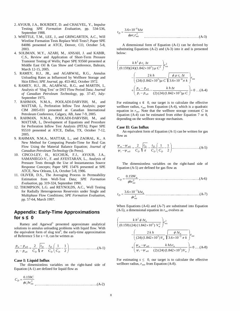
Appendix: Early-Time Approximations for s ≤ 0

Ramey and Agarwal5 presented approximate analytical solutions to annulus unloading problems with liquid flow. With the equivalent form of slug test6, the early-time approximation of Reference 5 for s = 0, can be written as

2

112

0

0

DD

DD

Dwi

ww

CC

tt

Cpp

pp

��...��.(A-1)

Case I: Liquid Influx

The dimensionless variables on the right-hand side of Equation (A-1) are defined for liquid flow as

2

159.0

watD

hrc

CC

,��..��..�.(A-2)

2

6106.3

watD

rc

tkt

.��....��.��(A-3) A dimensional form of Equation (A-1) can be derived by

substituting Equations (A-2) and (A-3) into it and is presented below:

2a23

2

)10)(1.842(0.159)(24

w

t rC

tchk

wat r

k

tc

C

hk

106.3

)101.842( )24(

263

0 )10842.1( )24( )2(

3

0

0

C

thk

pp

pp

wi

ww

�(A-4)

For estimating s ≤ 0, our target is to calculate the effective wellbore radius, rwa, from Equation (A-4), which is a quadratic equation in rwa. Note that the wellbore storage constant C in Equation (A-4) can be estimated from either Equation 7 or 8, depending on the wellbore storage mechanism.

Case II: Gas Influx

An equivalent form of Equation (A-1) can be written for gas flow as

2

112

0

0

DD

DD

Dwi

ww

CC

tt

C

..��.(A-5)

The dimensionless variables on the right-hand side of Equation (A-5) are defined for gas flow as

2

159.0

wa

wD

hr

VC

,��.��..��.��..�.(A-6)

2

3106.3

wa

aD

r

tkt

.��..�....��..��(A-7)

When Equations (A-6) and (A-7) are substituted into Equation (A-5), a dimensional equation in rwa evolves as

2a2

w3

2

)101.842 ( (24) (0.159)

w

a rV

thk

waa

w

rk

t

V

hk

106.3

)101.842( )24(

233

0 )101.842( )24( )2(

3

0

0

w

a

wi

ww

V

thk

.�(A-8)

For estimating s ≤ 0, our target is to calculate the effective wellbore radius, rwa, from Equation (A-8).

9

0.00 0.20 0.40 0.60 0.80 1.00

Time , h

0

500

1000

1500

2000

2500

3000

Pres

sure , kP

a

0

7

14

21

28

35

42

Gas R

ate , 103m

3/d

Total Test

Data ChartPERFORATION INFLOW TEST SHALLOW GAS RESERVOIR

EXAMPLE 1

pdataqgas

t 0.85 hpdata 2286 kPa


FIGURE 1: Pressure data and calculated gas influx rate in Example 1.

10-4 10-3 10-2 10-1 1.0 1012 3 4 5 6 7 89 2 3 4 5 6 7 8 9 2 3 4 5 6 7 89 2 3 4 5 6 7 89 2 3 4 5 6 7 8

ta , h

10-7

10-6

10-5

10-4

10-3

10-2

10-1

2

4

7

2

4

7

2

4

7

2

4

7

2

47

2

4

7

Der

ivative

, 1

06kP

a2/

Pa.s

Der ivative

Diagnostic Analysis

PERFORATION INFLOW TEST SHALLOW GAS RESERVOIR

EXAM PLE 1

Derivative data

Radial 0

k 85.962 mDp* 2297 kPa

Slope 2

s' 2.865

Approximate Start Of Radial Flow

t 0.43 hp 2274 kPa

FIGURE 2: PITA derivative for flow regime identification in Example 1.

0123456

1 / ta , hr-1

0.460

0.470

0.480

0.490

0.500

, 10

6kP

a2/

Pa.

s

2208

2231

2255

2278

2301

p , kP

a

Late Tim e

Diagnostic Analysis


EXAMPLE 1

data

Analysis 1

k 85.962 mDp* 2297 kPaVw 5.790 m3

h 1.000 m t 20.00 %rw 0.091 m

t 0.85 hp 2286 kPa


t 0.43 hp 2274 kPa

FIGURE 3: Analysis of late-time data in Example 1.

0.000 0.002 0.004 0.006

ta , h

0.00

0.02

0.04

0.06

, 10

6 kPa2

/Pa.

s

0133

266

398

531

664

797

p , k

Pa

Ear ly Tim e

Diagnostic Analysis


EXAMPLE 1

data

Analysis 1

s' 2.865

FIGURE 4: Analysis of early time data in Example 1.

10

0.00 0.20 0.40 0.60 0.80 1.00 1.20

Time , h

0

500

1000

1500

2000

2500

3000

Pre

ssur

e ,

kPa

0

7

14

21

28

35

42

Gas

Rate , 1

03m

3/d

Total Test

PITA ModelPERFORATION INFLOW TEST SHALLOW GAS RESERVOIR

EXAMPLE 1

pdatapmodelqgas

pwo (syn) 107 kPaP (avg) 2295 kPa



kh 85.00 mD.mk 85.000 mDsd -1.200t 20.00 %Vw 5.790 m3

h 1.000 mrw 0.091 m

FIGURE 5: Modeling of pressure data in Example 1.

10-4 10-3 10-2 10-1 1.0 1012 3 4 5 6 7 8 9 2 3 4 5 6 7 89 2 3 4 5 6 7 89 2 3 4 5 6 7 89 2 3 4 5 6 7 8

ta , h

10-7

10-6

10-5

10-4

10-3

10-2

10-1

2

4

7

2

4

7

2

4

7

2

4

7

2

4

7

2

4

7

Derivative ,

10

6 kPa

2 /P

a.s

Deriv ativ e


EXAMPLE 1

DerivativedataDerivativemodel

pwo (syn) 107 kPaP (avg) 2295 kPa


t 0.43 hp 2273 kPa

kh 85.00 mD.mk 85.000 mDsd -1.200t 20.00 %Vw 5.790 m3

h 1.000 mrw 0.091 m

FIGURE 6: Matching of PITA derivative data in Example 1.

0123456

1 / ta , hr -1

0.460

0.470

0.480

0.490

0.500

0.510

, 1

06kP

a2/

Pa.s

2208

2227

2247

2266

2285

2305

2324

p , k

Pa

Late Time


EXAMPLE 1

data model

pw o (syn) 107 kPaP (avg) 2295 kPa

kh 85.00 mD.mk 85.000 mDsd -1.200 t 20.00 %Vw 5.790 m3

h 1.000 mrw 0.091 m


t 0.43 hp 2273 kPa

t 0.85 hp 2286 kPa

FIGURE 7: Matching of late-time data in Example 1.

0 2 4 6 8

Time , h

1600

1800

2000

2200

2400

Pre

ssure

, k

Pa

10

14

18

22

26

Gas R

ate

, 103m

3/d

Total Test

Storage-Skin ModelFLOW & BUILDUP TEST SHALLOW GAS RESERVOIR

EXAMPLE 1a

pdatapmodelqgas

pi (syn) 2296 kPapav g 2296 kPa

kh 200.00 mD.mh 1.000 m

k 200.000 mDsd 0.380

t 7.21 h t 4.71 hpdata 2286 kPa

FIGURE 8: Modeling of drawdown and buildup test data in Example 1a.

11

10-3 10-2 10-1 1.0 1012 3 4 5 6 7 8 2 3 4 5 6 7 8 2 3 4 5 6 7 8 2 3 4 5 6 7 8

Pseudo-Time , h

10-3

10-2

10-1

1.0

2

3

4

6

8

2

3

4

6

8

2

3

4

6

8

, 10

6 kPa

2 /Pa.

s

Typecurv e

Storage-Skin ModelFLOW & BUILDUP TEST SHALLOW GAS RESERVOIR

EXAMPLE 1a

data

model

Derivativedata

Derivativemodel

pi (syn) 2296 kPapav g 2296 kPa

kh 200.00 mD.mh 1.000 m

k 200.000 mDsd 0.380

t 4.71 hp 2286 kPa

FIGURE 9: Pseudo-pressure and derivative match of buildup data in Example 1a.

0 1 2 3 4 5 6 7 8 9

Tim e , h

0

5000

10000

15000

20000

25000

30000

Pre

ssure

, kP

a

0.00

0.20

0.40

0.60

0.80

1.00

1.20

Gas R

ate , 103m

3/d

Total Te st

Data Chart

PERFORATION INFLOW TEST TIGHT GAS RESERVOIR

EXAM PLE 2

pdataqgas


FIGURE 10: Pressure data and calculated gas influx rate in Example 2.

10-4 10-3 10-2 10-1 1.0 101 1022 3 4 5 6 78 2 3 4 5 6 78 2 3 4 5 6 78 2 3 4 5 6 7 8 2 3 4 5 6 7 8 2 3 4 5 6 78

Pseudo-Time , h

10-5

10-4

10-3

10-2

10-1

1.0

101

102

103

2

4

8

2

5

2

4

9

2

48

24

8

2

4

8

2

5

2

4

9

Der

ivat

ive

, 10

6kP

a2/

Pa.

s

De rivative

Diagnostic Analysis

PERFORATION INFLOW TEST TIGHT GAS RESERVOIR

EXAMPLE 2

Derivativedata

Radial 0

k 0.003 mDp* 30780 kPa

Slope 2

s' 1.066


0.000.200.400.600.80

1 / ta , hr-1

20

30

40

50

60

, 10

6kP

a2/

Pa.

s

16535

18736

20937

23137

25338

27539

29740

31941

p , kP

a

Late Time

Diagnostic Analysis PERFORATION INFLOW TEST TIGHT GAS RESERVOIR

EXAMPLE 2

data

Analysis 1

k 0.003 mDp* 30780 kPaVw 0.454 m3

h 2.100 m t 10.00 %rw 0.150 m

t 7.96 hp 27648 kPa

FIGURE 12: Analysis of late-time data in Example 2.

12

0.00 0.01 0.02 0.03 0.04

ta , h

1.20

1.60

2.00

2.40

2.80

, 10

6 kPa2

/Pa.

s

3874

4219

4564

4908

5253

5597

5942

p , kP

a

Early Tim e

Diagnostic Analysis PERFORATION INFLOW TEST TIGHT GAS RESERV OIR

EXAMPLE 2

data

Analysis 1

s' 1.066

FIGURE 13: Analysis of early-time data in Example 2.

0 1 2 3 4 5 6 7 8 9

Time , h

0

6000

12000

18000

24000

30000

36000

Pre

ssure

, k

Pa

0.00

0.20

0.40

0.60

0.80

1.00

1.20

Gas R

ate

, 103m

3/d

Tota l Test

PITA ModelPERFORATION INFLOW TEST TIGHT GAS RESERVOIR

EXAMPLE 2

pdatapmodel

qgas


kh 0.02 mD.mk 0.011 mDsd 1.932 t 10.00 %

Vw 0.450 m3

h 2.100 mrw 0.150 m



10-4 10-3 10-2 10-1 1.0 101 1022 3 4 5 6 7 2 3 4 5 6 7 2 3 4 5 6 7 2 3 4 5 6 7 2 3 4 5 6 78 2 3 4 5 6 78

Pseudo-Time , h

10-5

10-4

10-3

10-2

10-1

1.0

101

102

103

104

2

5

2

5

2

5

2

5

2

5

2

5

2

5

2

5

2

5

Der

ivativ

e , 10

6 kPa2

/Pa.s

Deriv ativ e


EXAM PLE 2

Derivativedata

Derivativemodel


kh 0.02 mD.mk 0.011 mDsd 1.932 t 10.00 %

Vw 0.450 m3

h 2.100 mrw 0.150 m

t 7.93 hp 27628 kPa

FIGURE 15: Matching PITA derivative data in Example 2.

0.000.200.400.600.80

1 / ta , hr -1

20

30

40

50

60

, 1

06 k

Pa

2 /Pa.s

16535

19103

21670

24238

26805

29373

31941

p , k

Pa

Late Time


EXAMPLE 2

data model


t 7.96 hp 27648 kPa

kh 0.02 mD.mk 0.011 mDsd 1.932 t 10.00 %

Vw 0.450 m3

h 2.100 mrw 0.150 m

FIGURE 16: Matching of late-time data in Example 2.

13

0 200 400 600 800 1000

Time , h

0

5000

10000

15000

20000

25000

30000

35000

Pre

ssur

e , kP

a

0

10

20

30

40

50

60

70

Gas R

ate

, 103m

3/d

Total Test

Storage-Skin ModelPOST-FRAC FLOW & BUILDUP TIGHT GAS RESERVOIR

EXAMPLE 2a

pdata

pmodel

qgas

p i (syn) 31480 kPapav g 31472 kPa

kh 0.06 mD.mh 2.100 m

k 0.029 mDsd -3.562

t 845.88 h t 681.14 hpdata 30480 kPa

t 164.74 h t 28.59 hpdata 2341 kPaqg 5.876 103m3/d

FIGURE 17: Modeling of post-frac drawdown and buildup test data in Example 2a.

10-2 10-1 1.0 101 102 103 1042 3 4 5 6 78 2 3 4 5 6 78 2 3 4 5 678 2 3 4 5 678 2 3 4 5 6 7 2 3 4 5 6 78

Pseudo-Time , h

10-2

10-1

1.0

101

102

103

2

4

7

2

4

7

2

4

7

2

46

23

5

8

, 10

6 kPa2

/Pa.

s

Typecurv e

Storage-Skin ModelPOST-FRAC FLOW & BUILDUP TIGHT GAS RESERVOIR

EXAMPLE 2a

data

model

Derivativedata

Derivativemodel

pi (syn) 31480 kPapavg 31472 kPa

kh 0.06 mD.mh 2.100 m

k 0.029 mDsd -3.562

t 681.14 hp 30480 kPa

FIGURE 18: Pseudo-pressure and derivative match of post-frac data in Example 2a.

0 200 400 600 800 1000 1200 1400 1600 1800

Time , h

0

2000

4000

6000

8000

10000

Pre

ssu

re ,

kPa

0.00

0.20

0.40

0.60

0.80

1.00

Liq

uid

Rate , m

3/d

Total Tes t

Data ChartPERFORATION INFLOW TEST TIGHT COALBED M ETHANE RESERV OIR

EXAM PLE 3

pdata

qw ater


FIGURE 19: Pressure data and calculated water influx rate in Example 3.

10-3 10-2 10-1 1.0 101 102 103 1042 3 4 5 67 2 3 4 5 67 2 3 4 5 67 2 3 4 5 67 2 3 4 5 67 2 3 4 5 67 2 3 4 5 6 8

t , h

10-3

10-2

10-1

1.0

101

102

103

104

105

106

107

2

5

2

5

2

5

2

5

2

5

2

5

25

2

5

25

2

5

Der

ivat

ive

, kP

a

Derivative

Diagnostic Analysis PERFORATION INFLOW TEST TIGHT COALBED METHANE RESERVOIR

EXAMPLE 3

Derivative data

Radial 0

k 0.006mDp* 8858kPa

Slope 2

s' 1.095


14

0 200 400 600 800 1000 1200 1400 1600 1800

Time , h

0

2000

4000

6000

8000

10000

Pre

ssure

, k

Pa

0.00

0.20

0.40

0.60

0.80

1.00

Liq

uid

Rate , m

3/d

Total Test

PITA ModelPERFORATION INFLOW TEST TIGHT COALBED METHANE RESERVOIR

EXAMPLE 3

pdatapmodelqwater

pw o (syn) 90 kPap* 8237 kPa

kh 0.46 mD.mk 0.046 mDsd 1.336h 10.000 m

t 1.00 %Vu 0.01014 m3/mrw 0.091 m


10-3 10-2 10-1 1.0 101 102 103 1042 3 4 567 2 3 4 5 67 2 3 4 5 67 2 3 4 5 67 2 3 4 5 6 8 2 3 4 5 6 8 2 3 4 5 6 8

t , h

10-2

10-1

1.0

101

102

103

104

105

106

107

108

109

92

6

2

6

2

6

2

6

2

6

2

6

2

6

2

6

2

6

2

6

2

6

Deriva

tive

, kP

a

Deriv ativ e

PITA ModelPERFORATION INFLOW TEST TIGHT COALBED METHANE RESERVOIR

EXAMPLE 3


pwo (syn) 90 kPap* 8237 kPa

kh 0.46 mD.mk 0.046 mDsd 1.336h 10.000 m

t 1.00 %Vu 0.01014 m3/mrw 0.091 m

FIGURE 22: Matching PITA derivative data in Example 3.

10- 4 10-3 10-2 10-1 1.0 101 1022 3 4 5 6 78 2 3 4 5 6 78 2 3 4 5 6 78 2 3 4 5 6 78 2 3 4 5 6 78 2 3 4 5 6 78

Real Time , h

10- 2

10- 1

1.0

101

102

103

104

2

4

7

2

47

2

4

7

2

47

2

47

2

47

Der

ivative , kP

a

Derivative

PITA Model - Vw = 0.5 m3PERFORATION INFLOW TEST TIGHT COALBED METHANE RESERVOIR

EXAMPLE 3a


pw o (syn) 90 kPap* 8237 kPa

kh 0.46 mD.mk 0.046 mDsd 1.336

t 1.00 %h 10.000 mrw 0.091 m


t 4.59 hp 8179 kPa

Simulated Pressure Response With Downhole Shut-in

t 10.79 hp 8213 kPa

FIGURE 23: A test-design scenario for downhole shut-in of well in Example 3a.

0.0

0.5

1.0

1.5

2.0

0 5 10 15 20 25 30

Radius, m

dq/d

lnD t

, 103 m

3/d

t = 0.2 hrst = 0.5 hrst = 0.85 hrs

FIGURE 24: Rate Kernel (Region of investigation) for Example 1.

15

10-4 10-3 10-2 10-1 1.0 101 1022 3 4 5 6 78 2 3 4 5 6 78 2 3 4 5 6 78 2 3 4 5 6 78 2 3 4 5 6 78 2 3 4 5 6 78

Pseudo-Time , h

10-7

10-6

10-5

10-4

10-3

10-2

10-1

5

2

4

8

2

4

8

2

4

8

2

4

8

2

4

8

2

4

8

2

4

Der

ivat

ive

, 10

6kP

a2/

Pa.

s

Derivative

Induced Measurement NoisePERFORATION INFLOW TEST SHALLOW GAS RESERVOIR

EXAMPLE 1

Derivativedata

Derivativemodel

Der ivative w ithout Noise

FIGURE 25: Measurement noise appearing as late-time unit slope on the PITA derivative plot.

Documents

Use of PITA for Estimating Key Reservoir … PAPER 2006-172 Use of PITA for Estimating Key Reservoir Parameters N.M.A. RAHMAN, M. POOLADI-DARVISH, M.S. SANTO, L. MATTAR Fekete Associates