Use of an aptitude test in university entrance: a validity ... of an aptitude test in university entrance: a validity study ... Chris Whetton Researchers: ... Use of an Aptitude Test

Use of an aptitude test in

university entrance: a validity study

Final Report

Catherine Kirkup

Rebecca Wheater

Jo Morrison

Ben Durbin

Marco Pomati

September 2010

Use of an aptitude test in university entrance:

a validity study

Final Report

Catherine Kirkup

Rebecca Wheater

Jo Morrison

Ben Durbin

Marco Pomati

National Foundation for Educational Research

September 2010

Acknowledgements

The project team for this report consisted of:

Project director:

Chris Whetton

Researchers:

Catherine Kirkup and Rebecca Wheater

Project Administration Assistant:

Margaret Parfitt

Statistics Research and Analysis Group:

Jo Morrison, Ben Durbin and Marco Pomati

The NFER also gratefully acknowledges the advice given by members of the project steering

group and the assistance of the College Board and Educational Testing Services for providing

and scoring the SAT Reasoning TestTM

.

This project is co-funded by the Department for Business, Innovation and Skills, the Sutton

Trust, the National Foundation for Educational Research and the College Board.

Any opinions, findings and conclusions or recommendations expressed in this material are

those of the author(s) and do not necessarily reflect the views of the Department for Business,

Innovation and Skills, the Sutton Trust or the College Board.

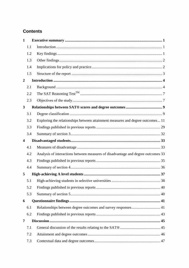
Contents

1 Executive summary ...................................................................................................... 1

1.1 Introduction ............................................................................................................... 1

1.2 Key findings .............................................................................................................. 1

1.3 Other findings ............................................................................................................ 2

1.4 Implications for policy and practice .......................................................................... 2

1.5 Structure of the report ............................................................................................... 3

2 Introduction .................................................................................................................. 4

2.1 Background ............................................................................................................... 4

2.2 The SAT Reasoning TestTM

...................................................................................... 7

2.3 Objectives of the study .............................................................................................. 7

3 Relationships between SAT® scores and degree outcomes ...................................... 9

3.1 Degree classification ................................................................................................. 9

3.2 Exploring the relationships between attainment measures and degree outcomes ... 11

3.3 Findings published in previous reports ................................................................... 29

3.4 Summary of section 3 .............................................................................................. 32

4 Disadvantaged students.............................................................................................. 33

4.1 Measures of disadvantage ....................................................................................... 33

4.2 Analysis of interactions between measures of disadvantage and degree outcomes 33



5 High-achieving A level students ................................................................................ 37

5.1 High-achieving students in selective universities ................................................... 38



6 Questionnaire findings ............................................................................................... 41

6.1 Relationships between degree outcomes and survey responses .............................. 41


7 Discussion .................................................................................................................... 45

7.1 General discussion of the results relating to the SAT® .......................................... 45

7.2 Attainment and degree outcomes ............................................................................ 46

7.3 Contextual data and degree outcomes ..................................................................... 47

7.4 Conclusion ............................................................................................................... 49

8 References ................................................................................................................... 50

Appendix 1: Methodology .................................................................................................. 53

A1.1 Participation ............................................................................................................ 53

A1.2 Data matching ......................................................................................................... 53

A1.3 Surveys .................................................................................................................... 54

Appendix 2: Student samples and background characteristics ...................................... 55

A2.1 Overview of the main sample.................................................................................. 55

A2.2 Background characteristics of each destination sub-sample .................................. 57

A2.3 Attainment scores .................................................................................................... 58

Appendix 3: Statistical outputs from the multilevel ordered categorical models .......... 59

Appendix 4: Measuring the goodness of fit of ordered categorical models ................... 80

List of Tables

Table 3.1 Degree classification outcomes for the 2009 graduate sample ............................ 9

Table 3.2 Multilevel ordered categorical regression of degree classification showing

significant variables ............................................................................................ 15

Table 3.3 Multilevel ordered categorical regression of degree classification comparing

average and total A level points scores............................................................... 17

Table 3.4 Multilevel ordered categorical regression comparing GCSE and SAT® subject

scores as predictors of degree classification ....................................................... 24

Table 5.1 Degree classification outcomes for high-achieving A level students ................ 37

Table 5.2 Multilevel ordered categorical regression of degree classification by type of

university ............................................................................................................ 39

List of Figures

Figure 3.1 Probability of degree outcome based on A level performance .......................... 19

Figure 3.2 Probability of degree outcome based on GCSE performance ........................... 20

Figure 3.3 Probability of degree outcome based on SAT® Maths performance ................ 21

Figure 3.4 Probability of degree outcome based on the UNIdiff value .............................. 25

Figure 3.5 Probability of degree outcome by school type (based on model 2 from Table

3.2)………………………………………………………………………………27

1

1 Executive summary

1.1 Introduction

In 2005, the National Foundation for Educational Research (NFER) was commissioned to

evaluate the potential value of using an aptitude test (the SAT Reasoning TestTM

) as an

additional tool in the selection of candidates for admission to higher education (HE). This

five-year study was co-funded by the Department for Business, Innovation, and Skills (BIS),

the NFER, the Sutton Trust and the College Board. This report presents findings from the

final phase of the project, relating the prior attainment and SAT® scores of participating

students who graduated in 2006 to their degree outcomes. It also summarises findings from

the study as a whole, and cross references where appropriate to the various interim reports.

1.2 Key findings

The primary aim of the study was to examine whether the addition of the SAT® alongside A

levels is better able to predict HE participation and outcomes than A levels alone.

Of the prior attainment measures, average1 A level points score is the best predictor of

HE participation and degree class, followed by average GCSE points score. The

inclusion of GCSE information adds usefully to the predictive power of A levels.

In the absence of other data, the SAT® has some predictive power but it does not add

any additional information, over and above that of GCSEs and A levels (or GCSEs

alone), at a significantly useful level.

Two other issues to be addressed in the study were: whether the SAT® can identify

economically or educationally disadvantaged students with the potential to benefit from HE

whose ability is not adequately reflected in their A level results; whether the SAT® can

distinguish helpfully between the most able applicants who get straight A grades at A level.

There is no evidence that the SAT® provides sufficient information to identify

students with the potential to benefit from higher education whose ability is not

adequately reflected in their prior attainment.

The SAT® does not distinguish helpfully between the most able applicants who get

three or more A grades at A level. The SAT® Reading and Writing components do

add some predictive power for some classes of degree at highly selective universities2,

but add very little beyond the information provided by prior attainment, in particular

prior attainment at GCSE.

1 The average points score for A levels was based on the QCDA system in which an A level grade A is

equivalent to 270 points, B grade is 240 points, etc. For GCSEs, grade G is equivalent to 16 points and an A*

grade is equal to 58 points. 2 For simplicity, in this report we refer only to universities. However, university includes any higher education

institution offering degree level courses.

2

1.3 Other findings

In addition to the key findings relating to the use of the SAT®, other findings about the

relationships between prior attainment and HE participation and outcomes emerged from an

analysis of the data.

The relationship between degree performance, prior attainment and the type of school

attended suggests that on average students from comprehensive schools are likely to

achieve higher degree classifications than students with similar attainment from

grammar and independent schools.

Having controlled for prior attainment, gender was not a significant predictor of

degree outcome, e.g. male students were neither more likely nor less likely to do

better at university than female students with the same prior attainment. In this

sample, ethnicity was also not a significant predictor of degree class, although in a

recent much larger study ethnicity differences were found to be statistically

significant (HEFCE, 2010a).

In an earlier phase of the research it was found that girls are more likely to be in HE

than boys with similar attainment, yet girls tend to enter courses with lower entry

requirements than would be expected from their prior attainment compared with boys.

1.4 Implications for policy and practice

The findings from this research support the following issues in relation to admission to HE:

For applicants who already have A level and GCSE attainment data, the SAT® would

not provide any additional information that would be useful for predicting degree

outcomes.

Tests used in the admission of candidates to HE should be investigated to ensure they

are valid predictors of undergraduate performance.

The use of data about the educational context in which students have obtained their

qualifications, particularly the type of school attended, should be encouraged when

comparing the attainment of HE candidates.

The importance of A level performance in predicting HE outcomes suggests that, due

to some inequalities in the reliability of predicted grades, a post-qualification system

may be more equitable and useful in assisting in the selection of candidates.

In assessing candidates for HE, average performance in both GCSE and A level

examinations is more important than the total points accumulated.

3

Other means of differentiating between high ability HE applicants may need to be

used (use of UMS3 marks) but the validity of this approach should be investigated.

See section 7 for a fuller discussion of these issues.

1.5 Structure of the report

Section 2 provides the background to the research and the aims of the study. The key findings

are described in more detail in sections 3 to 6 and the report concludes with a discussion of

the findings and the implications for policy and practice in section 7. The methodologies

employed, a full description of the representation of the sample and further technical data (the

outputs of the various analyses referred to in the report) are presented in appendices 1 to 4.

3 In the current system, A levels are graded from A* to E. The raw marks in individual papers are converted to

marks on a Uniform Mark Scale (UMS), so that comparisons across different subjects and different awarding

bodies can be made.

4

2 Introduction

In 2005, the NFER was commissioned to evaluate the potential value of using an aptitude test

as an additional tool in the selection of candidates for admission to higher education (HE).

For the purposes of the study, the SAT Reasoning TestTM

(also known as the SAT®) was

chosen because an earlier pilot (McDonald et al., 2001), using an earlier version of this test,

had found it to be an appropriate test to use with UK students and to have some potential for

such a purpose. This five-year study was co-funded by the Department for Education and

Skills (now the Department for Business, Innovation, and Skills), the National Foundation for

Educational Research (NFER), the Sutton Trust and the College Board.

This report presents findings from the final phase of the project, relating prior attainment and

SAT® scores to degree outcomes for a group of participating students who graduated in

2009. It also summarises findings from the study as a whole, with cross references where

appropriate to the various interim reports.

2.1 Background

Most UK applicants to higher education (HE) are selected on the basis of their attainment at

the end of compulsory education and their predicted or actual attainment in post-compulsory

education, For these students, A levels remain the most frequently taken academic

qualifications and are the basis on which the vast majority of candidates apply for university

admission.

This study stemmed largely from issues surrounding admission to higher education (HE) and

some of the limitations of the current system raised in the report by the Admissions to Higher

Education Steering Group, chaired by Professor Steven Schwartz (Admissions to Higher

Education Steering Group, 2004). These issues included the desire to widen participation in

HE, fair access and possible improvements to the admissions system. At the commencement

of this study, although the number of students benefiting from higher education (HE) had

increased substantially over previous years, some groups were still significantly under-

represented. A report into participation in higher education over the period 1994-2000

(HEFCE, 2005) noted that young people living in the most advantaged 20 per cent of areas

were five or six times more likely to go into higher education than those from the least

advantaged 20 per cent. Over the period of the study considerable changes have occurred,

including the establishment of the Office for Fair Access (OFFA), an independent, non

departmental public body, to promote and safeguard fair access to higher education for under-

represented groups. Recently HEFCE (2010b) reported ‘sustained and substantial’ increases

in the proportions of young people from disadvantaged areas entering HE and a narrowing of

the gap between the most advantaged and least advantaged areas. However, the gap in

participation rates between the most and least disadvantaged students remains significant.

There are also some concerns about fair access to the most selective universities (OFFA,

2010).

Offers of HE places are usually made primarily on the basis of prior attainment and predicted

A level examination results. The Schwartz report expressed a concern that although ‘prior

5

educational attainment remains the best single indicator of success at undergraduate level’

(p. 5), the information used to assess university applicants might not be equally reliable. In

other words, it was generally recognised that, for some students, their true potential might not

be reflected in their examination results due to social or educational disadvantages.

A related issue was that of access to highly selective courses and higher education

institutions. As the demand for university places generally exceeds the supply, HE

institutions must make choices between similarly highly qualified individuals. Prior to the

introduction of the new top A level grade, the A*, this was proving to be extremely difficult

for some HE admissions departments, with an increasingly large number of candidates

achieving A grades at A level. In response to this, a number of HE institutions had introduced

supplementary admissions tests or assessments for courses where the competition for places

was particularly fierce.

The Schwartz group recommended that assessment methods used within the admissions

system should be reliable and valid. Among its wider recommendations the Schwartz report

encouraged the commissioning of research to evaluate the ability of aptitude tests to assess

the potential for higher education:

Admissions policies and procedures should be informed and guided by current

research and good practice. Where possible, universities and colleges using

quantifiable measures should use tests and approaches that have already been shown

to predict undergraduate success. Where existing tests are unsuited to a course’s

entry requirements, institutions may develop alternatives, but should be able to

demonstrate that their methods are relevant, reliable and valid. (Admissions to

Higher Education Steering Group, 2004, p. 8)

A levels are central to the higher education admissions process and the ability of A level

grades to predict degree outcomes has been demonstrated using a large data set (Bekhradnia

and Thompson, 2002). Other studies have questioned the strength of the relationship between

A level attainment and degree outcomes and suggested that this can vary according to the

type of HE institution and the area of study (Peers and Johnston, 1994). However, there was

insufficient recent evidence regarding the predictive validity of a general admissions or

aptitude test within the UK context.

In the United States there is no national curriculum and there are no nationally recognised

academic qualifications equivalent to GCSEs or A levels. Admission to colleges is on the

basis of school grades (the high school grade point average) plus one or more college

entrance tests, the most common of which are the SAT® and the ACT® test4. High school

grades are considered a ‘soft’ measure because grading standards can vary widely from

school to school and from state to state, hence the need for a standardised admissions test.

The SAT Reasoning TestTM

(previously known as the Scholastic Assessment Test) is

therefore taken by high school students to provide information for colleges alongside their

4 Originally, ‘ACT’ stood for American College Testing. In 1996 the official name of the organisation was

shortened to simply ‘ACT’.

6

high school grade point average and SAT® results are used by universities to help compare

students from different parts of the US.

In a review of studies examining the ability of the SAT® to predict a number of measures of

success in college (including graduation), the combination of high school records and SAT®

scores were consistently the best pre-admission predictors (Burton and Ramist, 2001). As

might be expected, several studies showed that post-admission data (such as first year grades)

predicted graduation better than pre-admission measures because the predictors are closer in

time to the criterion of interest. However, despite the problems inherent in establishing

predictive validity, in particular range restriction and unreliability of grading standards,

unadjusted studies showed moderate correlations between SAT® scores and graduation

ranging from 0.27 to 0.33 (i.e. higher SAT® scores were generally associated with higher

graduation outcomes).

More recently, the College Board (Mattern et al., 2008) reported on a study conducted

examining the validity of the SAT® using a nationally representative sample of first-year

college students who had been admitted with the revised version of the test (the same one

used in this study). The correlations between high school grade point average (HSGPA) and

first year college grade point average (FYGPA), corrected for restriction of range, were 0.54

for female students and 0.52 for male students. Correlations between the SAT® and FYGPA

ranged from 0.52 to 0.58 for females and 0.44 to 0.50 for males. Combining the three

sections of the SAT® with HSGPA resulted in multiple correlations of 0.65 and 0.59

respectively.

Although high school grades are often seen as the slightly better predictor of college grades,

Kobrin et al (2002) reported that the SAT® adds to their predictive power to a statistically

significant degree, and may be a more accurate predictor for some groups of students with

discrepancies between high school grades and SAT® scores.

In Sweden, both school grades and scores on the Swedish Scholastic Aptitude Test

(SweSAT) are used to select students for admission to higher education. For each course of

study between a third and two-thirds of the places available are assigned on the basis of

grades, and the rest on the basis of SweSAT scores. Taking the SweSAT is entirely voluntary,

and it may be taken any number of times, with the highest achieved score being used.

Gustafsson (2003) reported that grades have better predictive validity than tests but that tests

can contribute to prediction when there are differences in the quality of education or when

grades suffer from lack of comparability.

The principal study underpinning this current research was the pilot comparison of A levels

with SAT® scores conducted by NFER for The Sutton Trust in 2000 (McDonald et al., 2001)

using a previous version of the SAT®. This small study revealed that the SAT® was only

modestly associated with A level grades, suggesting that they were assessing somewhat

distinct constructs. Analysis of item level data showed that the SAT® functioned similarly

for English and American students and found little evidence of bias in the SAT® items. A

further perceived advantage was that, as the results of the SAT® were provided as a scaled

score (at that time with a range of 400-1600), it would allow greater discrimination between

students than A level grades. On the basis of this pilot, it was considered worthwhile to carry

7

out further research to investigate what potentially useful information the SAT® might

provide to HE admission departments.

2.2 The SAT Reasoning TestTM

The content of the SAT® was revised in 2005 and it was this most recent version that was

used in this study. It comprises three main components: Critical Reading, Mathematics and

Writing. In the US the administration of the SAT® is split into ten separately timed sections,

with a total test time, excluding breaks, of three hours and forty-five minutes.

The Critical Reading section of the SAT® contains two types of multiple-choice items:

sentence completion questions and passage-based reading questions. Sentence completion

items are designed to measure students’ knowledge of the meanings of words and their

understanding of how sentences fit together. The reading questions are based on passages that

vary in length, style and subject and assess vocabulary in context, literal comprehension and

extended reasoning. The Mathematics section contains predominantly multiple-choice items

but also a small number of student-produced response questions that offer no answer choices.

Four areas of mathematics content are covered: number and operations; algebra and

functions; geometry and measurement; and data analysis, statistics and probability. The new

Writing section (first administered in the US in 2005) includes multiple-choice items

addressing the mechanical aspects of writing (e.g. recognising errors in sentence structure and

grammar) and a 25 minute essay on an assigned topic.

In the current study, no changes were made to any of the questions but one section was

removed (a section of new trial items which do not contribute to the US students’ scores)

giving a total of nine sections and an overall test time of three hours and twenty minutes.

Both in the McDonald study (McDonald et al., 2001) and in the current study, the results

indicated that the individual SAT® items functioned in an appropriate way for use with

English students.

2.3 Objectives of the study


levels is better able to predict HE participation and outcomes than A levels alone. Two

specific issues were also to be addressed, namely:

Can the SAT® identify students with the potential to benefit from higher education whose

ability is not adequately reflected in their A level results because of their (economically or

educationally) disadvantaged circumstances?

Can the SAT® distinguish helpfully between the most able applicants who get straight A

grades at A level?

Interim reports were published in 2007 and 2009 (Kirkup et al., 2007, 2009). In the 2007

report the analysis of the attainment data focused on the broad relationships between SAT®

scores and total scores at A level and GCSE. It also presented information from two student

surveys. The 2009 report focussed on three issues: further exploration of the relationships

8

between SAT® scores and attainment in particular individual A level subjects; analysis of the

2006 entry data, using UCAS5 data and combined HESA

6 and ILR

7 data; statistical modelling

of the background data of students to create more sensitive measures of economic and

educational disadvantage. A further brief report (Kirkup et al., 2010) updated the findings

from the analysis of the destination data to include students who entered higher education in

2007 and reported on a survey of participating students and young people carried out in

December 2008.

This report focuses on the overall objectives of the study. It is based on an analysis of the

degree outcomes of those participating students who entered HE in 2006 and completed

three-year degrees in 2009.

5 Universities and Colleges Admissions Service

6 Higher Education Statistics Agency

7 Individualised Learner Record

9

3 Relationships between SAT® scores and degree outcomes



Relationships between SAT® scores and participation in HE were described in the 2009 and

2010 reports and are summarised in section 3.3. Relationships between degree class and

measures of prior attainment, including the SAT®, are reported below.

Over 9000 students participated initially in the current study and took the SAT® in autumn

2005. Of this original group, just over 8000 participants were matched to their A level results

in 2006. A total of 2754 participating students entered HE in 2006 on three-year degrees and

graduated in 2009 and a further group of approximately 3800 participants were still studying

within HE. The background characteristics of the various sub-samples are broadly similar.

(See appendices 1 and 2 for a full description of the methodology and the representation of

the various sub-samples.)

3.1 Degree classification

The degree classification outcomes for the 2754 students who graduated in 2009 are shown in

Table 3.1 together with a comparison of classification outcomes nationally.

Table 3.1 Degree classification outcomes for the 2009 graduate sample

Graduate sample National

Class of degree Frequency Per cent Per cent

First class honours 326 11.8 11.1

Upper second class honours (2:1) 1613 58.6 55.1

Lower second class honours (2:2) 714 25.9 29.3

Third class honours 73 2.7 3.3

Other (pass, unclassified honours, ordinary,

degree without honours etc.) 28 1.0 1.2

Total 2754 100.0 100.0

Notes: the national population represents graduates from all UK HEIs who commenced their first degree in

2006-07 aged 18 and completed year 3 of a full-time first degree course in 2008-09 (HESA data from 2008/09).

Compared with a nationally representative population of graduates, matched by age, entry,

length of course and number of years of study, the graduate sample has a slightly higher

proportion of first class and upper-second class degrees. This is not unexpected given that the

10

overall prior attainment of the main study sample was higher than a comparable national

population8.

Having established the degree outcomes for the graduate sample, the main issue to be

examined was whether the SAT® added to the predictive power of A levels and GCSEs.

The first step in the analysis was to carry out some simple descriptive statistics looking at the

relationships between the various prior attainment measures and the class of degree obtained.

For this and subsequent analyses, third class degrees and below (other degrees such as

ordinary degrees, unclassified degrees, etc) were grouped together because of the relatively

small numbers of these in the sample. In order to calculate these simple correlations, the

degree classes were treated as interval data on a simple scale using 1 for a third class degree,

2 for a 2:2 degree, 3 for a 2:1 degree and 4 for first-class honours. (For the more complex

analyses the degree classes were more accurately considered as ordinal data - see section 3.2

below.) All the correlations were positive and statistically significant.

Significant correlations with degree class (in order of size) were:

• average9 A level points score (0.38)

• average KS4 (GCSE) points score (0.36)

• total A level points score (0.34)

• total KS4 points score (0.28)

• mean SAT® score (0.26) – the average of the scaled scores for the three separate

SAT® components

• SAT® Writing score (0.26)

• SAT® Reading score (0.24)

• SAT® Maths score (0.18)

These correlations are relatively modest due, in part, to the restricted range of the degree

classification scale, and the restriction in the prior attainment of the graduate sample. (The

study was restricted to students taking two or more A levels and the prior attainment of the

main study sample was higher than the national sample of such students – see sample

description in appendix 2.) Correlations are also generally weaker when there is a longer time

interval between the predictors and the criterion. The highest correlations were between class

of degree and average point scores for both A levels and GCSEs. The correlation between

8 For the mean prior attainment scores of the graduate sample and a comparison with the main sample and other

sub-sample, see Table A2.3 in appendix 2. 9 The average points score for A levels was based on the Qualifications and Curriculum Development Agency

(QCDA) system in which an A level grade A is equivalent to 270 points, B grade is 240 points, etc. For GCSEs,

grade G is equivalent to 16 points and an A* grade is equal to 58 points.

11

degree and average GCSE performance is somewhat surprising. It might be expected that

degree outcome would correlate much more highly with A level examinations, which were

taken two years closer to the degree outcome and which probably reflect a closer connection

with the subject area of the degree studied. The GCSE correlation suggests a significant

association between degree class and a student’s overall breadth of study and attainment and

therefore an important role for GCSEs in predicting performance in HE (see also section

3.2.2).

3.2 Exploring the relationships between attainment measures and degree outcomes

A number of regression analyses were then carried out in order to look simultaneously at the

relationships between the main attainment and background variables and to identify which of

these can predict degree outcomes. It was decided to use ordered categorical models,

specifically multilevel ordered categorical models, which model the statistical probability of

being in a particular category (e.g. having a first class degree). The reasons for using

multilevel ordered categorical models for this type of analysis and an explanation of how to

interpret the outcomes are given below.

A multilevel model is one which takes into account the hierarchical structure of data;

in this case students are clustered within universities. It might be expected that on

average students will be more similar to other students at the same university than

they are to students at other universities. Multilevel modelling allows this to be taken

into account, and provides more accurate estimates of coefficients and their standard

errors (hence ensuring that we can correctly determine whether an effect is

statistically significant or not).

Ordered refers to the fact that the outcomes of interest (degree results) can be placed

in a definite order or rank. A first is better than a 2:1, which is better than a 2:2, and

so forth. This differentiates it from unordered data, for example favourite colour.

However, whilst degree outcomes are ordered, they are not on an interval scale;

rather, they are categorical. An interval scale is one where the difference between

each successive outcome is equal, for example years: the time between 2009 and 2010

is the same as that between 2008 and 2009. This cannot be said of degree outcomes –

the difference between a first and a 2:1 is not necessarily the same as the difference

between a 2:1 and a 2:2.

Interpreting outputs: When categorical data is used in modelling, this is done by making

comparisons between the different categories, for example comparing boys to girls. This is

simple when there are only two categories, and requires only one equation. However, in our

case there are four categories, with an order, which for each model requires three separate

equations predicting:

1. the probability of achieving a third / other degree rather than a 2:2 or higher (OE1)

2. the probability of achieving a 2:2 or lower rather than a first or a 2:1 (OE2)

12

3. the probability of achieving a 2:1 or lower rather than a first (OE3).

Note that in each case these models consider the probability of achieving a given outcome,

versus that of achieving a better outcome. This means that a positive coefficient relates to

higher chances of the inferior outcome, and a negative coefficient relates to a lower chance of

the inferior outcome. This can be confusing, and so although the findings are the same, the

Original Equations (OE1, OE2 and OE3) have been reversed in the main report for ease of

interpretation.10

The outputs from the models are presented in full in appendix 3.

The reversed equations can be expressed as follows:

1. the probability of achieving a 2:2 or higher rather than a third / other degree (E1)

2. the probability of achieving a first or a 2:1 rather than a 2:2 or lower (E2)

3. the probability of achieving a first rather than a 2:1 or lower (E3).

Common versus separate coefficients: In an ordered categorical model it is possible to

include variables as either ‘common’ or ‘separate’ across the three equations. By including

them as common it is assumed that the impact of that variable on the chances of improved

degree outcomes is the same at all levels (chances of a first, 2:1, 2:2 or third); separate

coefficients enable the impact to vary between equations. Having a common coefficient is

desirable as interpretation is easier. Variables were initially included separately across all

three equations, but where the resulting coefficients were sufficiently similar the model was

updated to include just one common coefficient, for example the grammar and independent

school variables.

Goodness of fit: In a linear regression model, the R2 statistic is calculated as a measure of the

goodness of fit and can be interpreted as the proportion of the variation in outcomes which is

explained by the model. (In other words to what extent degree class is predictable from the

variables included in the model - A level scores, GCSE scores, SAT® scores, etc.) However,

for categorical models it is not possible to calculate an R2 statistic (intuitively, the difficulty

becomes clear when one considers what could be meant by the ‘proportion of variation in

outcomes’ for a categorical outcome). Instead a pseudo-R2 such as McFadden’s R

2 is used

which, whilst being calculated in a very different manner to the normal R2, is analogous to it,

in that it is a measure of the goodness of fit of the model. McFadden’s R2 is expressed as

values between zero and one (higher values indicating a more robust model and a better set of

predictors); however it cannot be interpreted as the proportion of variation explained by the

model. A rule of thumb is that values between 0.2 and 0.4 indicate a very good model fit11

.

Note that because of its reference to a base model12

, values should only be compared across

models that share a common base (i.e. they include the same set of students). For example,

10

The reason that the models were run ‘the wrong way around’ was that there were too few students achieving a

third to use this as the reference category, which meant that the models would not converge. 11

See http://www.soziologie.uni-halle.de/langer/pdf/papers/rc33langer.pdf 12

See appendix 4 for an explanation of how McFadden’s R2 is calculated.

http://www.soziologie.uni-halle.de/langer/pdf/papers/rc33langer.pdf

13

this means that values should not be compared between the Maths and non-Maths subject

models in Table 3.2 (models 6 and 7 respectively).

So, taking as an example the coefficients for SAT® ‘English’ from Model 1 in Table 3.2,

these are positive and significant for all three equations. This means that a higher SAT®

‘English’ score is associated with a higher degree outcome, regardless of what degree you

would otherwise be expected to have achieved. The coefficients for Maths SAT®, on the

other hand, suggest that Maths SAT® has no impact on the chances of achieving a third

versus higher (ns = non significant); however it points to a lower chance of achieving a 2:1 or

higher (versus a 2:2 or lower), and a higher chance of achieving a first (versus a 2.1 or

lower). So, a high Maths SAT® score is associated with a higher chance of achieving a high

or low degree outcome (a first or a 2:2/third) as opposed to a 2:1. The impact of attending a

grammar school or an independent school on degree outcome was similar across all three

equations and therefore these were included as common coefficients. In all of the models,

attending an FE college had no impact on the chances of achieving a 2:1 or higher (versus a

2:2 or lower), or a first (versus a 2.1 or lower) so it was removed from those equations. In

some models attending an FE college had an impact on the chances of achieving a third

versus higher and it was therefore included as a separate variable in the first equation of

each model. (In this model the impact is non-significant.)

The outcomes from the first set of models are summarised in Table 3.2. The outputs from

further models, focussing on disadvantaged students and able students, are described in

sections 4 and 5 respectively. Detailed statistical outputs for the models are given in appendix

3.

In some initial explorations of the data, it became apparent that it was not helpful to combine

the scores from the three components of the SAT®. The relationships between the Reading

14

and Writing components and degree classes were very similar, i.e. they were generally

predicting similar outcomes; but there was a different relationship between SAT® Maths

scores and degree classification. For most analyses, a combined SAT® ‘English’ variable

was created (from the mean of the Reading and Writing scores) with the SAT® Maths score

entered as a separate variable. In other models all three components (Maths, Reading and

Writing) were entered separately.

For GCSE performance, students’ average point scores were used rather than total point

scores. This was because the number of GCSEs taken can vary widely and may sometimes

reflect school policy and practice rather than the ability of the individual students. This effect

is much less pronounced at A level and therefore total A level points scores were initially felt

to be the most appropriate measure of A level performance. Most of the models therefore

included total A level points scores. However, the effect of substituting average A level

points scores for total A level points scores was also explored (models 2 and 3) and a detailed

comparison of these two models, similar in all other respects, is shown in Table 3.3.

Attainment data was taken from a dataset supplied to the NFER by the Department for

Children, Schools and Families (now the Department for Education). In this dataset, AS level

qualifications are included within the A level total points scores, using discounting rules to

avoid double counting qualifications13

. AS levels were not the focus of the study and were

not included separately in the analyses. Due to differences in the timing of some AS module

examinations and opportunities to re-sit AS modules in year 13, no attempt was made to

predict degree outcomes from qualifications achieved at the end of year 12.

13 http://www.education.gov.uk/performancetables/pilot16_05/annex.shtml

15

Table 3. 2 Multilevel ordered categorical regression of degree classification showing significant variables

All graduates Model 6

Maths subjs14

Model 7

Non-maths Model 1 Model 2 Model 3 Model 4 Model 5

Constant – equation 1 3.489 3.928 3.849 3.767 3.767 3.100 4.131

Constant – equation 2 1.043 1.280 1.259 1.240 1.214 0.977 1.337

Constant – equation 3 -2.091 -2.164 -2.090 -2.074 -2.120 -1.572 -2.231

E1 E2 E3 E1 E2 E3 E1 E2 E3 E1 E2 E3 E1 E2 E3 E1 E2 E3 E1 E2 E3

Average A level points (30) + + +

Total A level points (30) + + + + + + + + + + + +

Average KS4 points (6) + + + + + + + + + + + + ns + + + + +

SAT® ‘English’ (mean Reading and

Writing) score (10) + + + ns ns ns ns + ns ns + ns ns + ns ns ns ns ns + ns

SAT® Maths score (10) ns – + ns – + ns – + ns – + ns – + ns ns ns ns – ns

Prior attainment of university cohort

(UNIdiff )

ns + ns – – – – ns – ns ns – – ns – – ns – ns ns –

Grammar school attended ns – – – – – –

Independent school attended ns – – – – ns –

FE college attended ns - – ns – – ns

Sex ns ns ns ns ns ns ns

Asian ns

Black ns

Chinese ns

Sex / ethnicity interactions ns

Number of cases 2754 2754 2754 2754 2754 419 2335

Goodness of fit (McFadden’s R2)

15 0.12 0.74 0.64 0.57 0.53

Notes: + indicates a significant positive predictor; – indicates a significant negative predictor; ns indicates non-significant; shaded cells indicate variables not included in the model.

14

Mathematical and Computer Sciences; Physical Sciences; Engineering; Technologies 15

Values for models 6 and 7 are not given as they cannot be compared with models 1-5 – see appendix 4.

16

The findings from this analysis (models 1 – 7) are summarised below.

Findings relating to the SAT®:

Of the prior attainment measures, effect sizes revealed that average A level

performance had the strongest association with degree outcome, followed by average

GCSE point score. The inclusion of GCSE information adds usefully to the predictive

power of A levels.

In the absence of other data, the SAT® had some predictive power but it did not add

any additional information, over and above that of GCSEs and A levels (or GCSEs

alone), at a significantly useful level. This remained the case when the graduate

sample was divided into students studying ‘maths’16

subjects and students studying

‘non-maths’ subjects (models 6 and 7 in Table 3.2).

Other findings:

Students who had attended grammar schools or independent schools were less likely

to achieve as high a degree classification as might have be expected from their prior

attainment, i.e. they were likely to achieve a lower class of degree than students from

comprehensive schools with similar prior attainment.

Students who had attended FE colleges were more likely to achieve a third class

honours degree than students from comprehensive schools with similar prior

attainment.

Students at highly selective universities are likely to achieve a lower level of degree

than students at less selective universities with similar A level and GCSE attainment.

(‘Selectivity’ was measured by means of the UNIdiff value - the percentage of

students at a university with A level grades ABB or AAC or above – the higher the

value the more ‘selective’ the university.)

Having controlled for prior attainment, gender was not a significant predictor of

degree outcome, e.g. male students were neither more likely nor less likely to do

better at university than female students with the same prior attainment. In this

sample, ethnicity was also not a significant predictor of degree class, although in a

recent much larger study ethnicity differences were found to be statistically

significant (HEFCE, 2010a).

Each of these findings is explored in more detail in the sections that follow.

16

Mathematical and Computer Sciences; Physical Sciences; Engineering; Technologies

17

3.2.1 Predicting degree outcomes from A level performance

Table 3.3 shows the size of the coefficients from models 2 and 3 in Table 3.2, which model

the impact of including average A level points scores and total A level points scores

respectively.

Table 3.3 Multilevel ordered categorical regression of degree classification

comparing average and total A level points scores

Model 2 Model 3

E1 E2 E3 E1 E2 E3

Constant 3.928 1.280 -2.164 3.849 1.259 -2.090

Average A level points (30) 0.747 0.601 0.791

Total A level points (30) 0.089 0.068 0.042

Average KS4 points (6) 0.594 0.754 0.639 0.673 0.832 0.914

SAT® ‘English’ (mean Reading

and Writing) score (10) -0.001 0.014 -0.005 -0.003 0.018 0.004

SAT® Maths score (10) -0.009 -0.025 0.020 -0.018 -0.030 0.015

Prior attainment of university

cohort (UNIdiff ) -1.872 -0.582 -1.718 -1.292 -0.235 -1.156

Grammar school attended -0.415 -0.491

Independent school attended -0.734 -0.514

FE college attended -0.745 -0.798

Number of cases 2754 2754

Goodness of fit (McFadden’s R2) 0.74 0.64

Notes:

Significant coefficients are emboldened

E1 = equation 1 (the probability of achieving 2:2 or higher rather than a third / other degree)

E2 = equation 2 (the probability of achieving a first or a 2:1 rather than a 2:2 or lower)

E3 = equation 3 (the probability of achieving a first rather than a 2:1 or lower)

Scales were created for the A level and GCSE variables so that each increase in the scale was

equivalent to an increase of 1 grade, e.g. 30 pts at A level and 6 points for a change in GCSE

grade. The value of the coefficient therefore models the effect of a change of one grade. As

some of the variables are average point scores, great care must be taken in comparing the

relative size of the coefficients. For example, the coefficients for total A level points scores

18

represent the difference of a change of one grade in a student’s total A level points, (e.g.

achieving the points equivalent of AAB instead of ABB), whereas the coefficients for

average A level points scores represent a change of one grade in a student’s average, (e.g. an

average B points score from ABC or BBB instead of an average C from BCD or CCC). The

coefficient of the UNIdiff variable appears particularly large because it represents the

difference between a university with a UNIdiff value of 0 per cent (no students with A level

grades ABB or AAC or above) and a university with a UNIdiff value of 100 per cent (all

students with A level grades ABB or AAC or above). In reality most students will be at

universities nearer to the average figure for the sample.

The McFadden's R2

is the goodness of fit measure and shows how well the model fits the

data. The values for models 2 and 3 are 0.74 and 0.64 respectively. As all the other variables

in these two models are the same and they are based on the same students, this suggests that

average A level points score is a slightly more useful predictor of degree class than total A

level points score. By comparison with these two models, when SAT® scores are used

instead of A levels and GCSEs to predict degree class (model 1 in Table 3.2) the McFadden's

R2

is only 0.12, indicating a much weaker set of predictors. Models were also run using

GCSE and A levels separately (without SAT® scores) and the McFadden's R2

values were

0.37 (A level average performance + UNIdiff + school type) and 0.49 (GCSE average

performance + UNIdiff + school type). A fuller explanation of McFadden's R2

and the values

for all the models quoted in this report are given in appendix 4.

As mentioned previously, most models included a total A level points score variable because

this was initially felt to be the most appropriate measure of A level performance. When the

goodness of fit of each model was calculated, it was found that average A level point score

was a slightly more useful predictor of degree class than total A level point score. However,

the similarities in the McFadden's R2

values for these two models show that there is not a

great difference between using total or average A level points scores to predict degree class,

and it was therefore not considered necessary to re-run the models that had included the total

A level points score variable.

As shown in Tables 3.2 and 3.3, average A level points score was strongly associated with

degree class. Based on model 2 from Table 3.2, the probabilities of obtaining a particular

degree (e.g. a first rather than a 2:1 or lower; a 2:1 or a first rather than a 2:2 or lower; and a

2:2 or higher rather than a third or lower) based on average A level performance are

illustrated in Figure 3.1.

19

Figure 3.1 Probability of degree outcome based on A level performance

Figure 3.1 demonstrates the significant relationship between average A level performance

and the eventual class of degree obtained. The probability of obtaining an upper second or

first class degree increases from a probability of about 46 per cent for students with an

average E grade to 90 per cent for students with an average of an A grade. The probability of

achieving a first class degree increases from 15 percent for students with an average B grade

to 28 per cent for students with an average of an A grade at A level.

There was no significant difference between male and female students or between students

from different ethnic groups once prior attainment had been taken into account. This is

presumably because any differences (in this sample) are already reflected within their GCSE

and A level results.

0%

10%

20%

30%

40%

50%

60%

70%

80%

90%

100%

150 180 210 240 270

Pro

ba

bil

ity

Average A level

Above a third

2:1 or above

First

E D C B A

20

3.2.2 Predicting degree outcomes from GCSE performance

The relationships between degree outcome and A level performance and between degree

outcome and GCSE performance are very similar as illustrated in Figure 3.2. These

probabilities are based on model 2 from Table 3.2.

Figure 3.2 Probability of degree outcome based on GCSE performance

0%

10%

20%

30%

40%

50%

60%

70%

80%

90%

100%

40 46 52 58

Pro

ba

bil

ity

Average Key Stage 4

Above a third

2:1 or above

First

C B A A*

As can be seen from the figure above, the probability of getting a first class honours degree

rather than a 2:1 or below is around five per cent for student with an average of a grade C at

GCSE. The probability of achieving first class honours increases to eight percent with an

average grade B, 14 per cent with an average grade A and 24 per cent with an average grade

A*. There were 322 students in the graduate sample whose GCSE points average was 55 or

higher and, therefore, half or more of their GCSE grades were A* (including 52 students with

all A* grades - an average 58 points). At the lower end of the model, there were 403 students

with an average of grade C at GCSE, rounded to the nearest grade (i.e. an average GCSE

points score between 37 and 43). The remaining 1973 students were between these two

extremes.

21

3.2.3 Predicting degree outcomes from SAT® performance

The relationship between degree classification and SAT® scores was not straightforward, in

particular the relationship between degree class and the Maths SAT® component scores.

High Maths SAT® scores were associated with a higher chance of getting a first, but also a

higher chance of getting a 2:2 or less (see Figure 3.3). In other words the highest scores were

not always associated with the highest degree classes. When both A level and GCSE

performance were excluded (see model 1 in Table 3.2) ‘English’ SAT® scores (the average

of the SAT® Reading and Writing scores) had some predictive power across all degree

classes. However, when both A level and GCSE performance were included (model 3), high

‘English’ SAT® scores were associated only with a higher chance of getting a 2:1 or higher

rather than a 2:2 or less. In the model using average A level points score (model 2) the

‘English’ SAT® scores were not significant. Excluding A level scores from the model (see

model 4) did not affect the Maths SAT® coefficients. The coefficients for the ‘English’

SAT® became slightly larger (i.e. it became a slightly better predictor), but still only the 2:2

or less coefficient was significant.

Figure 3.3 shows the relationship between degree class and Maths SAT® scores, based on

model 2 from Table 3.2.

Figure 3.3 Probability of degree outcome based on SAT® Maths performance

0%

10%

20%

30%

40%

50%

60%

70%

80%

90%

100%

200 300 400 500 600 700 800

Pro

ba

bil

ity

SAT Maths Score

Above a third

2:1 or above

First

As can be seen in Figure 3.3, the probability of a student getting a first class honours

increases as the Maths SAT® score increases. However, the probability of getting an upper

second or above actually decreases (i.e. there is an increased probability of achieving a 2:2 or

below). So a student with a Maths SAT® score of 500 has a probability of about 78 per cent

22

of getting a 2:1 or above and around an 11 per cent probability of achieving a first. A student

with a much higher Maths SAT® score of 700 has a probability of about 15 per cent of

getting a first but the probability of getting a 2:1 or above drops to around 69 per cent. The

reasons for this are unclear. The Maths SAT® has no impact on the chances of achieving a

third versus higher; the coefficient was not significant.

Although the SAT® did not seem to offer any additional power in predicting undergraduate

success generally, further modelling of the data was used to ascertain whether the SAT®

components were more useful in predicting degree outcomes for particular subjects. In other

words, would SAT® Maths be useful for predicting ‘maths-related’ degree outcomes and

would ‘English’ SAT® be useful for predicting non-maths subjects? (In the USA, colleges

tend to base admission decisions on the most relevant SAT® components score(s) for the

subject of study. It was felt useful therefore to explore the potential utility of the SAT® at a

very broad maths / non-maths subject level, by splitting the sample into these two groups.) It

was not possible to explore the predictive power of the SAT® at a more specific level

because the number of students in some subject groups was too small. However, as can be

seen from models 6 and 7 in Table 3.3, which included students taking ‘maths-related’ and

‘non-maths’ degrees respectively, the majority of the SAT® coefficients were again non-

significant.

3.2.4 Predicting degree outcomes from specific GCSE or SAT® scores

In exploring the utility of the SAT® for predicting degree outcomes, there was some concern

that it was inappropriate to compare SAT® scores reflecting attainment in Reading, Writing

and Maths only with average GCSE performance, which reflects attainment over a much

larger range of subjects. Models predicting degree outcomes from performance in either

GCSE mathematics or GCSE English were therefore compared with models based on

performance in the relevant SAT® components (Reading, Writing or Maths). In all of these

models, average GCSE points score and total / average A level points score were excluded. A

summary of the results is shown in Table 3.4 and the detailed outputs from each model are

presented in appendix 3. By comparing effect sizes, GCSE mathematics scores and GCSE

English scores were found to be better predictors of degree class than SAT® Maths, SAT®

Reading or SAT® Writing scores.

Higher GCSE maths scores were associated with higher degree outcomes, ie the

higher the GCSE grade the higher the class of degree (model 8). Higher Maths SAT®

scores were associated with a higher chance of getting a first class degree only (model

9).

Higher GCSE English scores were associated with higher degree outcomes (model

11). Higher Reading SAT® scores were associated with a higher chance of getting a

2:1 or higher and of getting a first (model 12).

Without GCSE English data, higher Writing SAT® scores were also associated with

higher degree outcomes (model 15). However, when both GCSE English and Writing

SAT® scores were included (model 16), higher Writing SAT® scores were associated

23

only with a higher chance of getting a 2:1 or above and a higher chance of getting a

first. English GCSE remained associated with higher degree outcomes at all levels.

Having controlled for prior GCSE maths attainment, attending a grammar school or an

independent school was not a significant predictor of degree outcome (model 8). In other

words, students from grammar schools and independent schools were neither more likely nor

less likely to do better at university than students from comprehensive schools with the same

prior attainment. However, students from grammar schools and independent schools were

likely to do less well at university than students from comprehensive schools with the same

prior GCSE English attainment (model 11).

The difference in the significance of school type in the models for maths GCSE and English

GCSE could suggest school type has differential impact on the GCSE grades that students

obtain in these subjects. This could possibly be linked to entry policies for examinations (e.g.

tiered papers) and / or examination preparation. Grammar schools and independent schools

were not significant in the models predicting degree class based on SAT® performance

alone, possibly because there was no preparation for the SAT® and therefore no link between

SAT® scores and school type.

The possibility that the type of school attended has more impact on grades achieved in GCSE

English than grades achieved in GCSE mathematics has little significance in relation to

admissions to HE, given that it relates to two GCSE subjects only. It also emerges from a

relatively small study, the primary focus of which was the SAT®. However, it may be

something that could be investigated further as part of a wider exploration of the use of

contextual data.

Table 3.4 also shows that the pseudo-R2 values for these models are noticeably lower than

earlier models. While it is of interest to examine the interplay of the SAT® components and

English and maths GCSE scores, degree outcomes are better explained using overall GCSE

and A level point scores, as these measures contain more information about the ability of

students.

24

Table 3.4 Multilevel ordered categorical regression comparing GCSE and SAT® subject scores as predictors of degree classification

Model 8 Model 9 Model 10 Model 11 Model 12 Model 13 Model 14 Model 15 Model 16

Constant – equation 1 3.513 3.484 3.510 3.678 3.501 3.678 3.678 3.537 3.690

Constant – equation 2 1.052 1.022 1.052 1.144 1.052 1.150 1.144 1.078 1.156

Constant – equation 3 -2.038 -2.065 -2.055 -1.994 -2.037 -2.001 -1.994 -2.016 -1.992

E1 E2 E3 E1 E2 E3 E1 E2 E3 E1 E2 E3 E1 E2 E3 E1 E2 E3 E1 E2 E3 E1 E2 E3 E1 E2 E3

Maths KS4 points (6) + + + ns + +

English KS4 points (6) + + + + + + + + + + + +

SAT® Maths score (10) ns ns + ns ns +

SAT® Reading score (10) ns + + ns + +

SAT® Writing score (10) + + + ns + +

Prior attainment of university cohort (UNIdiff ) ns + + ns + ns ns + ns ns + + ns + + ns + ns ns + + ns + + ns + ns

Grammar school attended ns ns ns – ns – – ns –

Independent school attended ns ns ns – ns – – ns –

FE college attended – – – ns – ns ns – –

Number of cases 2625 2625 2625 2625 2625 2625 2625 2625 2625

Goodness of fit (McFadden’s R2) 0.00 0.01 0.06 0.29 0.02 0.33 0.29 0.06 0.32

Notes: + = significant positive predictor; – = significant negative predictor; ns = non-significant; shaded cells indicate variables not included in the model




25

3.2.5 Selective universities

As shown in Table 3.3, students attending highly selective universities - those with a high

percentage of students with A level grades ABB or AAC or above (a high UNIdiff value) -

were less likely to achieve as high a class of degree as students from less selective

universities with similar attainment.

Figure 3.4 illustrates impact of the UNIdiff measure on the probability of degree outcomes,

based on model 2 from Table 3.2.

Figure 3.4 Probability of degree outcome based on the UNIdiff value

0%

10%

20%

30%

40%

50%

60%

70%

80%

90%

100%

0 10 20 30 40 50 60 70 80 90

Pro

ba

bil

ity

University difficulty (%)

Above a third

2:1 or above

First

Percentage of first degree full-time students with AAC, ABB or above

The average UNIdiff value for the graduate sample was 35 percent (i.e. 35 percent of full-

time first degree students with A levels AAC or ABB or better). A student in the graduate

sample with average attainment17

at a university with an average UNIdiff value (e.g.

Loughborough) has a ten per cent probability of obtaining a first class degree. By comparison

a student with the same prior attainment at a university with a UNIdiff value of above 80 per

cent (e.g. Bristol or Imperial College) has less than a five per cent probability of obtaining a

first.

17

BBCC at A level and mostly Bs and some As at GCSE – see appendix 2.3

26

Using the UNIdiff measure is only one way of defining selective universities and it was

considered prudent to explore this finding in a different way. This was done by running two

regression analyses: comparing students at universities in the Russell Group18

with students

from other universities and comparing students at the Sutton Trust ‘Top 30’19

universities

versus other universities. Both of these analyses gave very similar results; for a student of

average attainment it was slightly easier to achieve a higher degree (e.g. a first versus lower)

in the ‘non-selective’ university group than in the highly selective group. As these were less

sophisticated analyses than the multilevel ordered categorical regression models, they are not

reported further.

Other potential difficulties in the interpretation of this particular finding had to be overcome.

Firstly, there were uneven numbers of students studying within the different broad subject

areas and differences between subject areas in the difficulty of obtaining specific degree

classes (e.g. first class degrees) could not be reflected in the model because of the small

numbers of students in some groups. In order to discover if the UNIdiff finding was common

to all subject areas, separate logistic regression models, predicting the probability of getting a

first versus any other class of degree, were run for students in each broad area of study

(biological sciences, historical and philosophical studies, etc). All of the significant subject

results showed an association in the same direction as the graduate sample as a whole. In

other words, when the broad subject areas of study were taken into account, it was still harder

for students with the same prior attainment to get a first at a university with a high UNIdiff

value.

A second difficulty was that the graduate sample included relatively large numbers of

students from independent and grammar schools who, in comparison with comprehensive

students, had achieved degrees lower than would have been expected from their prior

attainment (see 3.2.6 below). Although school type was taken into account in the modelling

of the data, it was considered important to ensure that the strength of the UNIdiff finding was

not overstated. A further model was therefore run excluding students who had attended either

independent schools or grammar schools. In this model the UNIdiff coefficients are similar,

and remain significant for equations 1 and 3. This indicates that, for a student of average

attainment either from a comprehensive school or an FE college, it is more difficult to obtain

a first class honours degree from a highly selective university (i.e. a university with a high

UNIdiff value) than a less selective one. Also, that a student is more likely to get a third class

degree, rather than a 2:2 or higher, at a highly selective university than a student with similar

attainment at a less selective one.

In almost all subject areas (14 out of 17), the Sutton Trust ‘Top 30’ universities actually gave

out proportionally more first class degrees within our sample than the ‘other’ universities, so

the UNIdiff finding is not simply due to fewer firsts being awarded at these highly selective

18

20 leading UK universities - see http://www.russellgroup.ac.uk/home 19

A list of highly selective universities in Scotland, England and Wales defined by the Sutton Trust

(http://www.suttontrust.com) as those with over 500 undergraduate entrants each year, where it is estimated that

less than 10 per cent of places are attainable to students with 200 UCAS tariff points (equivalent to two D

grades and a C grade at A-level) or less.

27

universities. It suggests that due to the large number of very able students competing for first

class honours, it is more difficult to obtain this classification in highly selective universities

than in less selective institutions. Although this finding goes beyond the objectives of the

study it emerged as a by-product of the main analysis and as such has been reported. To what

extent students are already aware of this when applying to universities is unclear and whether

they are nevertheless prepared to join such highly competitive environments due to the

‘market value’ of the degrees they obtain when they graduate.

3.2.6 Type of school or college attended

Another variable that has a significant impact on students’ degree outcomes is the type of

academic institution attended prior to university. The impact of school type on degree

outcome for a student of average attainment is shown in Figure 3.5. This figure is once again

based on model 2 from Table 3.2.

Figure 3.5 Probability of degree outcome by school type (based on model 2 from

Table 3.2)

Students from grammar schools or independent schools are likely to achieve a class of degree

that is slightly lower than students from comprehensive schools with similar prior attainment.

As can be seen in the figure above, the probability of students from comprehensive schools

(with average attainment for the graduate sample) obtaining a 2:1 or above is 78 per cent. For

28

students from grammar schools with similar attainment the probability is 70 percent and for

students from independent schools 63 per cent. Similarly, the probability of comprehensive

school students obtaining a first class degree is ten per cent. This drops to seven per cent for

similarly attaining students from grammar schools and only five per cent for similar students

from independent schools.

To look at this in another way, independent or grammar school students, who achieve the

same level of degree as students from a comprehensive school (with the same GCSE

attainment and other background characteristics), are likely to have an average A level grade

that is approximately 0.5 to 0.7 of a grade higher. Therefore a comprehensive student with

grades BBB is likely to perform as well at university as an independent or grammar school

student with grades ABB or AAB.

One perceived potential complication with this finding was the extent to which students from

the various types of schools were disproportionately distributed in the highly selective

universities. Students from independent schools and grammar schools tended on average to

attend universities with UNIDiff values that were significantly higher than those attended by

students from comprehensive schools or FE colleges. (The mean UNIdiff values by school

type were 55 per cent, 42 per cent, 25 per cent and 30 per cent respectively.). However the

model includes both the UNIDiff variable and school types meaning that there is still a

significant difference attributable to school type over and above what is accounted for by the

selectiveness of the university (UNIDiff). In other words, although independent and grammar

school students disproportionately go to more selective universities they still perform less

well than their peers. In one of the models reported later (section 5.1 and model 19 in

appendix 3), students from the most highly selective universities (the Sutton Trust Top 30)

were excluded, yet the grammar school and independent school coefficients were still

significant. In other words students from independent and grammar schools are performing

below expectations in other universities, not just the highly selective ones.

While there seems to be a persistent school type effect it is quite likely that it is a proxy for

some other difference between the types of school; one possibility being school achievement.

This issue was explored by removing the institution type variables (comprehensive schools,

grammar schools, etc) from model 2 (the model including average A level performance) and

adding schools’ average total GCSE points scores. School-level GCSE performance was also

found to be significantly associated with degree outcome; for students with the same prior

attainment from different schools, the higher the school’s performance the more likely these

students were to get a lower class of degree. The effect size of school-GCSE performance

was comparable with the effect size for grammar schools and FE colleges but less than the

effect size for independent schools. The McFadden’s R2 for this model was 0.67, which was

less than the original model with school type (R2 = 0.74). Adding institution types back in, as

well as school-level GCSE performance, resulted in the institution types being significant and

GCSE performance becoming non-significant. So school-level GCSE performance explains

less about degree outcomes than institution type.

29

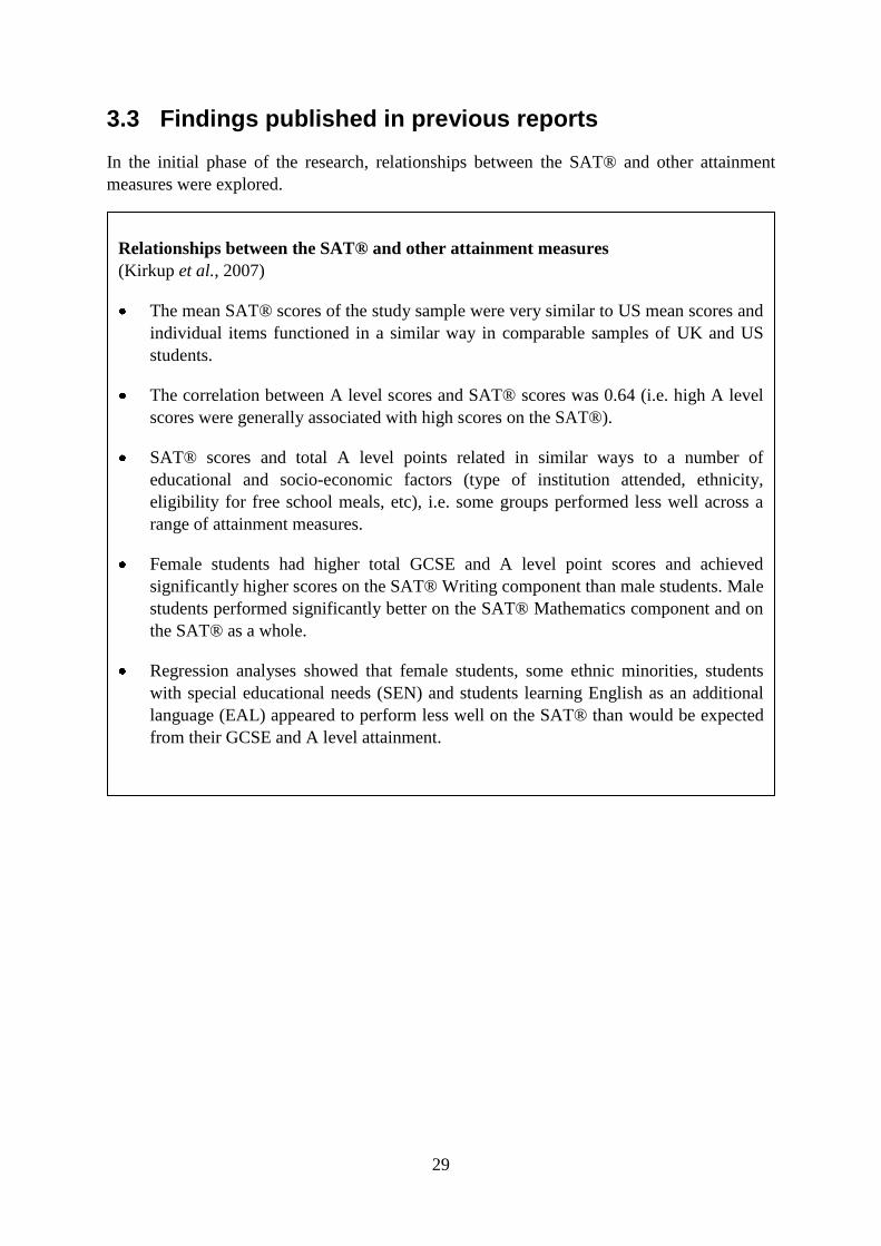
3.3 Findings published in previous reports

In the initial phase of the research, relationships between the SAT® and other attainment

measures were explored.

Relationships between the SAT® and other attainment measures

(Kirkup et al., 2007)

The mean SAT® scores of the study sample were very similar to US mean scores and

individual items functioned in a similar way in comparable samples of UK and US

students.

The correlation between A level scores and SAT® scores was 0.64 (i.e. high A level

scores were generally associated with high scores on the SAT®).

SAT® scores and total A level points related in similar ways to a number of

educational and socio-economic factors (type of institution attended, ethnicity,

eligibility for free school meals, etc), i.e. some groups performed less well across a

range of attainment measures.

Female students had higher total GCSE and A level point scores and achieved

significantly higher scores on the SAT® Writing component than male students. Male

students performed significantly better on the SAT® Mathematics component and on

the SAT® as a whole.

Regression analyses showed that female students, some ethnic minorities, students

with special educational needs (SEN) and students learning English as an additional

language (EAL) appeared to perform less well on the SAT® than would be expected

from their GCSE and A level attainment.

30

More detailed analyses examined the relationships between the components of the SAT® and

specific A level subjects.

Relationships between the SAT® and A level subjects (Kirkup et al., 2009)

The relationships between the SAT® components and A level subjects were not all the

same. SAT® Maths was more strongly related to A level grades in predominately

science based subjects whereas Critical Reading and Writing were more closely related

to subjects such as History and English A levels.

The mean SAT® scores associated with particular grades of A levels were at different

levels for different subjects. (For example, the mean SAT® Maths score of students

obtaining an A or B grade in Physics was over 600, whereas for Geography it was

around 500.) This could be seen as reflecting a difference in the difficulty of different

A level subjects.

Students studying A level mathematics achieved significantly higher SAT® Maths

scores compared with those students not studying A level mathematics. This increase

was similar for male and female students. The increase in SAT® Reading and Writing

scores for students studying English at A level (compared with those not taking

English) was somewhat greater for male students than for female students.

Over a number of different subject areas, male students tended to achieve higher

SAT® scores than female students with the same grade in the same A level subject.

There was some evidence that differences between male and female scores on the

SAT® were related to test-taking strategies, particularly differences in omission rates

on SAT® items.

31

A subsequent analysis phase explored the relationships between the various attainment

measures (including the SAT®) and participation in HE. The minimum entry points

requirement for each HE course was obtained (wherever possible) in order to evaluate

whether students had obtained places on courses commensurate with their prior attainment.

These relationships were first explored using 2006 HE entry data only and were subsequently

updated using combined 2006 and 2007 entry data (to include gap year students, deferred

entrants, etc).

Relationships between attainment and HE participation (Kirkup et al., 2010)

Performance at A level was the strongest predictor of participation in HE and of obtaining a

place on a ‘prestigious’ course with high entry point requirements. Prior attainment at

GCSE and SAT® scores were also significant. For students with similar A level and GCSE

attainment and similar background characteristics, but different SAT® scores, those with

higher SAT® scores were more likely to be in HE. Relationships between HE destinations

and students’ background characteristics were as follows:

Comparing participants in the study with similar prior attainment:

Girls were more likely to be in HE than boys.

Asian and Black participants were more likely to be in HE and Chinese participants less

likely to be in HE compared with White participants.

Participants with English as an additional language (EAL) were more likely to be in HE

than those with English as a first language.

Within HE, girls tended to enter courses with lower entry requirements than would be

expected compared with boys.

Asian students and EAL students tended to enter courses with higher entry requirements

than would be expected compared with white students and non-EAL students

respectively.

Students in grammar schools tended to enter less prestigious courses than would be

predicted from their attainment, while those in independent schools tended to achieve

places on more prestigious courses.

See also section 4.3.

32

3.4 Summary of section 3



As reported previously, higher SAT® scores are associated with participation in HE but less

strongly than either GCSEs or A levels.

‘English’ SAT® (mean Reading and Writing) scores correlate with degree classification

outcomes and in the absence of any other reliable measures could be used to give some

prediction of HE performance. However, the SAT® adds very little predictive power when

combined with GCSE data only and does not provide any additional predictive power when

both average A level and average GCSE performance are taken into account. Although the

currently available data from GCSEs and A levels does not always provide sufficient

information to resolve all HE admissions decisions, this research indicates that adopting the

SAT® would not provide a solution to predicting undergraduate success in the UK.

In addition to the main finding in respect of the SAT®, several other general findings have

emerged from modelling the degree outcome data. Some of these support research carried out

elsewhere.

The relationship between degree performance, prior attainment and the type of school

attended suggests that students from comprehensive schools are likely to do better in

HE than students with similar attainment from grammar and independent schools.

Girls are more likely to be in HE than boys with similar attainment, yet girls tend to

enter courses with lower entry requirements than would be expected from their

attainment compared with boys.

Neither gender nor ethnicity is significantly related to degree outcome, when prior

attainment is taken into account, e.g. male students are neither more likely nor less

likely to do better at university than female students with the same prior attainment.

See section 7 for a discussion of these and other issues arising from this research.

33

4 Disadvantaged students

One specific issue for the study to address was whether the SAT® could identify students

with the potential to benefit from higher education whose ability was not adequately reflected

in their A level results because of their (economically or educationally) disadvantaged

circumstances. In the past, an argument put forward for the SAT® is that it measures aptitude

rather than attainment and is therefore less dependent on a student’s socioeconomic

background and schooling – although the evidence does not unequivocally support this view

(see McDonald et al., 2001). In the McDonald study (using three samples of students from

low-attaining schools, high-attaining schools and independent schools), students were placed

into three bands on the basis of their mean A level scores. Within each band, SAT® test

scores tended to be lowest in the low-attaining schools and highest in the independent

schools. However, the relationship between A levels and the SAT® was not a strong one;

some students who scored highly on one measure did not do so on the other. It was reported

that using SAT® scores in addition to A levels as a basis for selection to HE would increase

the number of students considered for selection in all three samples. However, the percentage

increase in the number of students that would be considered was highest in the low-attaining

schools.

Assuming A levels do not adequately reflect the ability of some disadvantaged students, it

would be likely that such students might exhibit inconsistent performance, i.e. perform better

on the SAT® than in their A levels. Those who continue with further study would then be

expected to do better than would be predicted by their A levels in HE. The thinking here is

that it is only those with inconsistent performance who would be likely to benefit from the

introduction of SAT®; those whose overall performance is well-reflected by A level would

not be affected by the additional measure.

4.1 Measures of disadvantage

The measures available in this study to compare economic or educational disadvantage were

Free School Meal entitlement (FSM), the Income Deprivation Affecting Children Index

(IDACI), school-level GCSE performance and rates of progression into HE20

. If the SAT®

could help identify those with potential to benefit from higher education whose ability is not

adequately reflected in their A level results, we would expect to find that those from more

deprived backgrounds who did well on the SAT® but had less good prior attainment would

do better than expected at university.

4.2 Analysis of interactions between measures of disadvantage and degree outcomes

In order to see if the SAT® could identify those with the potential to benefit from HE,

interaction terms were added to one of the models. Interaction terms look at variables in

combination, in this case in pairs, to see if there is any differential relationship between them

20

the percentage of 18 year old students from a school / college who progress to HE

34

and degree outcome. For example, to examine how various measures of disadvantage, such as

eligibility for free school meals, interact with attainment measures and the resultant impact on

degree outcomes. Interactions between FSM, IDACI, sex, school-level GCSE performance,

school-level HE progression rates, with each of average GCSE scores, English SAT® and

Maths SAT® scores, were considered together with interactions between both English SAT®

scores and Maths SAT® scores with A level point scores. Interactions with prior attainment

(A level and GCSE) were included in the analysis so that we could ascertain whether the

SAT® can indicate potential for certain types of students (e.g. boys, those from deprived

areas, those from lower performing schools, those from schools that have lower HE

continuation rates, those who were eligible for FSM), over and above what is indicated by

their GCSE and A level scores.

Initially a model was constructed that included all the interaction terms, regardless of

statistical significance. As so many of the interaction terms were not significant, the model

was refined by removing those interactions that were furthest from being significant. As

many of the variables and interactions are closely related to each other, when some of these

non-significant interactions were removed from the model, changes to the behaviour of other

interactions occurred, going from being significant to being non-significant or vice versa (a

feature called co-linearity). Part of the process of modelling is to judge which ones to retain

and which to remove. In a final version of the model there was a significant interaction

between students’ average GCSE performance and school-level HE progression rates. This

shows that a student with a high GCSE score who attends a school from which many students

go on to HE is more likely to get a better class of degree than a student with a high GCSE

score from a school with fewer students continuing into HE. Alternatively, comparing

students from schools with similar HE progression rates, those with higher GCSE scores are

more likely to get better degrees.

Some of the interactions between SAT® scores and the various measures of disadvantage

were statistically significant but were not particularly robust due to the issue of co-linearity.

They were not retained in the final model. Students’ average GCSE performance as a stand-

alone variable was not a significant predictor of degree class. This is because, in this

interaction model, students’ GCSE performance is subsumed within the various interactions.

This shows that predicting degree class from prior attainment alone is not straightforward, as

attainment is mediated by many other factors.

The McFadden’s R2 of the final model was 0.66. This is slightly higher than the McFadden’s

R2 for model 3 (0.64) which is identical apart from the interaction terms. This indicates that

while statistically significant, the interaction terms are only adding a small amount of

additional information to the model.

The outputs from the final interaction model discussed above are presented in Table A3.17 in

appendix 3.

35


In earlier phases of the research, relationships between the SAT®, attainment and

background characteristics were explored. In these analyses it was found that performance on

the SAT® was not independent of social background.

Score differences between different groups on the SAT® are well documented but are also

found in most other measures of educational achievement (Camara and Schmidt, 1999). This

was also the case in the current study with differences in all the main attainment measures (A

levels, GCSEs and the SAT®) according to a number of different background variables (FSM

eligibility, ethnicity, EAL, etc).

Some analyses focussed on particular background characteristics associated with

disadvantaged circumstances. The first of these looked at performance on the SAT®.

Relationships between the SAT® and background characteristics (Kirkup et al.,

2009)

Two measures of affluence / deprivation were used: one (IDACI – Income Deprivation

Affecting Children Index) was from the Pupil Level Annual School Census (PLASC), and

the other was based on students’ questionnaire responses.

When prior attainment at GCSE was not taken into account, students from schools

with a higher IDACI index (i.e. from areas of low income households) did less well on

the SAT® than students from less deprived areas with similar A level attainment.

However, if prior attainment was included, students with similar A level and GCSE

points performed similarly on the SAT® irrespective of household income.

Using the affluence measure derived from the survey response, SAT® scores tended

to be higher for more affluent students (compared with less affluent students with

similar A level attainment). Scores were significantly higher on two components

(Reading and Writing) when prior attainment (average GCSE score) was taken into

account.

36

In a later phase of the research, the factors affecting participation in HE were explored, with a

particular focus on students in educationally or economically disadvantaged circumstances.


There is no evidence from the inclusion of interaction terms in the analysis that the SAT®

identifies those students with the potential to benefit from higher education whose ability is

not adequately reflected in their prior attainment. One difficulty with this analysis is that the

students who have completed degrees are those who went into HE immediately after school.

It was not possible to look at those students who did better than would be expected on the

SAT® given their A level results and did not continue into HE.

Relationships between attainment and HE participation (Kirkup et al., 2010)

Performance at A level was the strongest predictor of participation in HE and of obtaining

a place on a course with high entry point requirements. Prior attainment at GCSE and

SAT® scores were also significant. Relationships between HE destinations and

disadvantaged circumstances were as follows:

Comparing students in HE from maintained schools:

Students from more deprived areas were on average just as likely to be studying at

more prestigious institutions (or on courses for which there is fierce competition), as

students from less deprived areas with similar attainment and background

characteristics.

Comparing students in HE from both maintained and non-maintained schools (regression

analysis using an affluence measure based on students’ survey responses):

More affluent students were more likely to be studying on courses with high entry

point requirements than might be expected from their attainment.

Participation in HE was also related to school-level performance:

GCSE performance at school level was positively related to the entry points of

students’ HE courses; i.e. students from high performing schools were more likely to

achieve places on courses with high entry requirements than students from low

performing schools when comparing students with the same level of attainment.

For students with similar attainment from similar schools, those with higher SAT®

scores were more likely to have achieved places on courses with higher entry point

requirements than students with similar attainment but lower SAT® scores. The

difference in course entry points was greater between students from low-performing

schools compared with students from high-performing schools.

37

5 High-achieving A level students

As stated in section 2.3, one of the main aims of the research was to ascertain:


grades at A level?

In an earlier phase of the project it was discovered that there was considerable variation in the

SAT® scores of those students who had gained three or more A grades at A level. This

finding suggested that the SAT® might be useful to HE admissions staff to help them

differentiate between candidates from this high-ability group, should the SAT® prove to be a

valid predictor of degree outcomes.

In the graduate sample, 533 students had a minimum of three A grades at A level. The

degrees obtained by these high-achieving A level students are shown in Table 5.1.

Table 5.1 Degree classification outcomes for high-achieving A level students

Number of A grades at A level First 2:1 2:2 3rd /

other

Total

Three 72 206 25 4 307

Four 48 125 6 0 179

Five 12 25 3 0 40

Six 5 2 0 0 7

Total 137 358 34 4 533

Per cent 25.7 67.2 6.4 0.8 100

Graduate sample (per cent) 11.8 58.6 25.9 3.7 100

Due to rounding, percentages may not sum to 100.

As can be seen from the table above, the proportion of first class honour degrees awarded in

this group of students is much higher than in the graduate sample as a whole.

Having established that the SAT® added very little predictive power to that of A levels and

GCSEs in the general population (see section 3), the further issue to be explored was whether

the SAT® was more useful in predicting the degree outcomes of high ability students. If

higher SAT® scores were associated with higher degree class, then the variation in SAT®

test scores amongst this group might be helpful in the selection of applicants for HE.

Correlations were calculated between degree outcomes and the various measures of prior

attainment (including SAT® scores). Due to the small size of this sub-sample and the

restriction in the range of scores and degree outcomes, it was expected that these correlations

38

would be relatively small compared to the graduate sample as a whole (see section 3.1). The

correlations with degree class (in order of size) were:

• average A level points score (0.16)

• average KS4 (GCSE) points score (0.15)

• SAT® Writing score (0.11)

• SAT® Reading score (0.09)

• SAT® Maths score (0.09)

Unfortunately, due to the small number of students with three or more A grades and

insufficient variation in the degree outcomes it was not possible to use a multilevel ordered

categorical model for this particular group of students only; the model failed to converge21

.

Two alternative means of exploring this issue were devised; firstly using the whole graduate

sample and secondly using an alternative group of high-achieving A level students, as

described in section 5.1 below. A multilevel ordered categorical model was run using the

complete graduate sample, flagging those students who had three or more A grades at A level

and creating an interaction term for their SAT® scores. (The interaction indicates if there is a

differential relationship between the SAT® and degree outcomes for students with fewer than

three A grades compared with students with three or more A grades, i.e. does the SAT® tell

us anything more about one group or the other.) In this model, A level performance was

excluded because there would have been insufficient variation in students’ A level scores. As

might be expected, the higher the GSCE score the higher the class of degree students were

likely to achieve. In terms of the SAT® interaction, this was non-significant, suggesting that

the SAT® doesn’t seem to indicate anything about high-achieving A level students that isn’t

already encapsulated in their GCSE results.

5.1 High-achieving students in selective universities

As it was not possible to use a multilevel ordered categorical model for the 533 students with

three or more A grades only, it was decided to explore the predictive power of the SAT®

with a slightly larger group of ‘high ability’ students. For the purpose of this analysis the

graduate sample was split into two groups: students attending highly selective universities in

the Sutton Trust ‘Top 30’ (see definition in section 3.2.5) and students from all other

universities. The Sutton Trust ‘Top 30’ (ST30) group was chosen as an appropriate

alternative means of exploring the outcomes of high-achieving students due to the high entry

qualifications generally demanded for admission to these universities. The graduates in the

ST30 group were all relatively high ability A level students with 36 per cent of this group

21

Multilevel models, like many other statistical models, use an iterative algorithm to fit a model to the data. The

algorithm uses information about the relationships in the data to repeatedly refine the model. In cases where

there is insufficient information or inconsistency within the data, either due to too few cases or due to weak or

unstable relationships, the model cannot make the necessary refinements and does not converge to a stable

model definition.

39

having obtained three or more A grades and 77 per cent having obtained at least one A grade

(compared to three per cent and 24 per cent respectively in the ‘other universities’ group).

The ST30 group included 496 of the 533 graduates with three or more A grades at A level.

The model including graduates from the ‘other universities’ was run purely for comparison

purposes.

The coefficients of the models from the two groups are given in Table 5.2 and in Tables

A3.18 and A3.19 in appendix 3.

Table 5.2 Multilevel ordered categorical regression of degree classification by type

of university

Sutton Trust ‘Top 30’

Model 18

Other Universities

Model 19

E1 E2 E3 E1 E2 E3

Constant 4.364 1.899 -1.715 3.458 0.695 -2.478

Total A level points (30) 0.110 0.079 0.013 0.094 0.074 0.103

Average KS4 points (6) 1.081 1.156 1.130 0.371 0.570 0.590

SAT® ‘English’ (mean Reading and

Writing) score (10) -0.000 0.024 0.030 -0.008 0.008 -0.035

SAT® Maths score (10) -0.033 -0.051 0.018 -0.008 -0.012 0.021

Prior attainment of University cohort

(UNIdiff ) -3.435 -0.300 -1.961 -0.162 1.283 -0.482

Grammar school attended -0.515 -0.495

Independent school attended -0.532 -0.644

FE college attended -0.330 -1.004

Number of cases 1381 1373

Notes:

Significant coefficients are emboldened




The significant results for SAT® ‘English’ (the mean of the Reading and Writing

components) show that these SAT® components are adding some information to the

probability of achieving some types of degree class, but not consistently across different

40

degree classes for the Sutton Trust ‘Top 30’ (ST30) or the other universities. In comparison,

the coefficients for average KS4 points are much higher in both models and are associated

with degree class in a consistent direction. Comparison of effect sizes indicates that the

SAT® components are less useful indicators when looking at university outcome as whole,

after prior attainment at GCSE has been taken into account.

Average KS4 points scores have higher coefficients in the ST30 universities model compared

with the other universities model, and a comparison of effect sizes indicates that prior

attainment at GCSE has a stronger relationship with degree outcome at the more selective

universities compared with the other universities.


In the initial phase of the research, the extent to which the SAT® might distinguish helpfully

between the most able applicants who got straight As at A level was investigated. In these

analyses, a sub-group of students who achieved at least three A grades at A level was used;

three A grades having been chosen as the benchmark for the level required to gain entry to

some leading UK universities.


From these analyses, evidence indicates that the SAT® would not distinguish helpfully

between the most able applicants who get straight A grades at A level. The SAT®

components do add some information to the model for some classes of degree at highly

selective universities, but add very little beyond the information provided by prior attainment,

in particular prior attainment at GCSE.

Relationships between the SAT® and other attainment measures (Kirkup et al., 2007)

Students who had gained three or more grade As at A level achieved significantly

higher scores than the rest of the sample on all components of the SAT®. There was

considerable variation in the SAT® scores of this group offering the possibility of

differentiation between high ability HE candidates (had the SAT® proven to be a valid

predictor of degree outcomes).

Students who achieved very high SAT® scores were not always the same students

who achieved three or more A grades at A level and vice versa. Students who achieved

very high SAT® scores but did not form part of the ‘three A grades’ group tended to

be male students.

Some students, who might have failed to gain admission to the most prestigious

universities on the basis of their A level grades, nevertheless achieved scores in the top

15 per cent or even top five per cent of SAT® scores.

41

6 Questionnaire findings

The student surveys give some contextual data to the main findings. However, due to the

relatively small number of students in some of the survey sub-samples, in particular the 2008

survey, the findings must be treated with some caution.

Questionnaire data from the first two surveys in 2006 formed the basis of an affluence

measure that was used in much of the early research. This was useful for comparing students

from maintained schools with those from independent and FE colleges who did not appear on

PLASC and for whom we therefore did not have the same level of background information. It

is possible that any findings from this study may complement much larger ongoing research

focussing specifically on attitudes to HE (e.g. Futuretrack - http://www.futuretrack.ac.uk/).

6.1 Relationships between degree outcomes and survey responses

Of the 2754 students in the graduate sample, 2352 had taken part in the first 2006 survey

whilst still at school / college and 1290 had responded to the survey in autumn 2006 at the

start of their first year in HE.

Responses to some survey questions were examined to see if there were any significant

relationships between the types of response and the degree class obtained. These were just

simple cross-tabulations and therefore did not take any other variables, most notably prior

attainment, into account.

In the first survey, school / college students were asked if they had a specific job or career in

mind that they would like to do in the future, with a choice of four responses: absolutely

certain, fairly certain, unsure and no idea at all. It was hypothesised that students with a

clear career direction would be more certain about subject / course choices and more

motivated to do well at university. However, in the graduate sample those students who had

been uncertain or had no career in mind at the start of their course had actually performed

significantly better than those who had been absolutely or fairly certain about a job or career.

Of course, it is highly likely that some students’ career plans will have been formulated and

others abandoned during the intervening years. Having checked the attainment of the various

groups, it was found was that those seeking the academic challenge of HE without clear

career plans were the highest attaining group of students and therefore more likely to do well.

In the same survey, students were asked about the number of books in the home, a

characteristic of the home environment that is often associated with socio-economic status

(Clark and Akerman, 2006). As might be expected, those students with the largest reported

number of books in the home achieved proportionately more first class and upper second

class degrees than other groups of students.

In the second survey, having just started an HE course, students were asked if the place they

had obtained was their first choice, second choice or obtained through ‘clearing’22

. Those

22

UCAS service that helps students without a university place to find suitable vacancies on HE courses

http://www.futuretrack.ac.uk/

42

who had obtained their first choice place had achieved significantly more first class and upper

second class degrees than students who had taken a place that was either their second choice

or obtained through clearing. Those who had failed to get their first choice (or second choice)

had lower average attainment and had presumably not achieved the grades required for their

original choices. However, although the proportions were smaller, some students in each

group, including those who obtained places through clearing, had achieved first class degrees.

This suggests perhaps that some students with slightly lower A level grades may have done

better in HE than would have been expected.

Only 567 students in the graduate sample took part in the 2008 survey. The impact of

differences in students’ ratings of their universities and their enjoyment of HE on degree

outcomes was explored, but due to size of this sub-sample these findings must be treated with

caution.

In one section of the survey, students were asked whether they felt they had chosen the

correct university, the correct course of subject, and whether studying for a degree was a

worthwhile investment (using a three point scale of yes, not sure, no). Of these three,

choosing the correct course or subject was significantly associated with degree outcome;

those responding yes achieving proportionately more first class degrees. Students were also

asked to rate various academic aspects of their university (tuition, pastoral support, study

facilities and feedback on work or progress) using a five point scale from excellent to very

poor. The first three of these were not significantly associated with the class of degree

obtained but those who considered they had received feedback that was good or excellent had

received more first class or upper second degrees than the other groups.

43


As well as providing some background details about their home and family circumstances,

the first questionnaire in spring 2006 asked participating students about their experiences of

school or college in years 12 and 13, their immediate plans after A levels and their views of

higher education.

Findings from the spring 2006 survey – based on a maximum of 6825 students


Ninety-two per cent of the students who completed the survey indicated that they

would definitely or probably go to university in either 2006 or 2007.

About 60 per cent of the students were absolutely certain or fairly certain what job

they would like to do in the future. The most popular careers were medicine (15 per

cent); engineering, science and IT (14 per cent); health and social welfare (12 per

cent); and teaching (11 per cent).

The most popular reasons for applying to university were subjects / courses (86 per

cent), social life (65 per cent), career potential (65 per cent), requirement of chosen

career (63 per cent), earnings potential (58 per cent).

Over 120 institutions were cited as the preferred choice for higher education. The five

institutions most frequently cited were the universities of Manchester, Leeds,

Birmingham, Nottingham and Cambridge.

The most important reasons for selecting a particular university were: academic

reputation (75 per cent), facilities (74 per cent), location (67 per cent), social life (62

per cent), graduate employment prospects (49 per cent), best available course (48 per

cent).

Over 90 per cent of respondents indicated that their education in year 12 and year 13

had equipped them with useful skills and knowledge.

Over 80 per cent had been given helpful information about university but less than 50

per cent felt they had been given good information about jobs and training or

encouraged to look into vocational training.

Although the majority of students thought their school had prepared them for studying

at university, a sizeable proportion thought they were not very well prepared (24 per

cent) or not at all well prepared (4 per cent).

44

The second survey in autumn 2006 asked students about their immediate post school / college

situation and any current or future plans with regard to higher education.

The final survey (December 2008) addressed students’ views on life at university, asked them

to rate various aspects of their university and indicate how much time they had spent carrying

out various study and leisure activities.

Findings from the 2008 survey – based on a maximum of 1315 students in HE (Kirkup

et al., 2010)

There were some very large differences between students both in their reported term-time

activities and also in the ratings of their universities, e.g.:

the number of hours spent attending tutorials, lectures, etc and carrying out private

study (even allowing for some intentional misreporting)

the number of hours in paid employment during term-time

the amount / quality of pastoral care / support

the amount / quality of feedback on work / progress.

Approximately half of respondents reported at least one issue that had had a major impact

on their likely degree classification and 18 per cent had asked for such issues to be taken

into consideration.

Students with higher prior attainment scores appeared to have enjoyed HE the most.

Findings from the autumn 2006 survey – based on a maximum of 3177 students


Over three quarters of the autumn survey sample (approximately 2500 students) had

started a course at an HEI in autumn 2006. Approximately 300 students planned to take

a gap year, with a guaranteed or deferred place for autumn 2007, and approximately 400

had no immediate plans to enter HE.

Eighty-six per cent of students in HE had obtained their first choice of university,

six per cent had gained their second choice and eight per cent had obtained a place

through the clearing system.

Approximately 60 per cent of the students in HE had commenced three-year courses

and a further 30 per cent were on four-year courses.

Over 95 per cent were fairly confident or very confident of their ability to complete the

course.

45

7 Discussion

The objectives of the study were to investigate the following:

Can the addition of the SAT® alongside A levels better predict HE participation and

outcomes than A levels alone?

Can the SAT® identify students with the potential to benefit from higher education whose

ability is not adequately reflected in their A level results because of their (economically or

educationally) disadvantaged circumstances?


grades at A level?

The conclusion from the current research study is the SAT® is unable to meet any of the

above aims in any significantly useful way. Other emerging findings described in the

previous sections may have possible implications for future HE admissions policy and

practice.

7.1 General discussion of the results relating to the SAT®

Establishing the predictive validity of measures used to predict future performance is by no

means straightforward and this was made particularly difficult in this study for a number of

unchangeable considerations. The range of the criterion, the degree classification, was

extremely restricted, with very few students obtaining below an upper-second class degree.

The score ranges of the predictor variables were also severely restricted because the graduate

sample was a relatively high ability group and those who did not go into HE were obviously

excluded from the graduate outcome analysis. Thus some variation in the test scores was lost.

It is also likely that there is lack of comparability in the degree classifications across different

courses and institutions, although this was controlled for to some extent by the multilevel

structure and the inclusion of the UNIdiff measure.

Partly as a result of the restricted ranges of the predictors and the criterion, the correlations

between the various pre-admission measures and degree outcomes were relatively weak. The

SAT® was a weak predictor of degree outcomes. The best predictors of degree class were

average performance in A level and GCSE examinations. Having taken these into account the

SAT® did not add to the predictive power of the model to any significant degree.

One reason for the failure of the SAT® to add any significant predictive power is that it is

possible that the underlying constructs assessed by the SAT® and A levels are now too

similar. In an earlier study reported in 2001 (McDonald et al., 2001) using an earlier version

of the SAT®, it was concluded that it was assessing a somewhat distinct construct from A

levels. Changes to the SAT® in 2005, with the introduction of the essay and some higher

order maths items, may have weakened the underlying difference between the SAT® and A

levels. In 2007, Cambridge Assessment mapped the content of the SAT® against GCSE

papers in English and mathematics (higher tier) and concluded that much of the content of the

SAT® is included in the National Curriculum programmes of study for English and

46

mathematics (Cambridge Assessment, 2007). It may be that despite changes to the content of

the SAT® and some overlap with GCSE and A level content, it is still not as good a predictor

of undergraduate performance as nationally produced curriculum-based qualifications that are

closer in content to UK university courses.

Whatever the reason, it is clear that the SAT® is not predicting graduate outcomes in any

way that suggests it would be helpful in identifying young people who would do well at

university (assuming they already have A level and GCSE data). Despite considerable

variation in SAT® scores between HE applicants with similar A level attainment, this

variation has not proved to be useful in predicting degree outcomes. Other aptitude or

admissions tests may also differentiate between applicants in terms of test scores but such

differentiation may not be helpful in predicting undergraduate success. Aptitude tests or other

admissions tests may well be useful in contexts where other attainment data is lacking.

However, the use of any admission test needs to be validated; supported by evidence that it is

a reliable and valid measure of HE performance.

7.2 Attainment and degree outcomes

One of the initial reasons for undertaking this study was that it was hoped to offer additional

information to assist HE admissions departments in selecting those candidates who would

perform well at university. In particular, it was hoped it would help the admissions

departments of highly selective universities (where the demand for places far exceeds the

supply available) to differentiate between equally highly qualified students. Since the start of

this study there has been a change in the A level qualifications available with the introduction

of the A*. Although this may reduce the ceiling effect to some extent, it may not resolve the

issue for some highly selective courses and universities. Another way to differentiate between

A level students (particularly for students with one or more A* grades) would be to offer

universities UMS marks, indicating the variation in actual marks underlying equivalent

grades. However, the extent to which this information might be useful in predicting degree

outcomes requires further investigation. The variation in A level marks within such a

restricted range of ability may not add sufficient predictive power to be meaningful.

Although the SAT® does not appear to offer any help as an additional indicator of degree

performance, some of the supplementary findings emerging from this study lend support to

some previous research findings and add to a body of evidence that may be useful in guiding

future policy and practice.

Firstly, this study suggests that the strongest predictor of degree performance is average

performance at A level (slightly better predictor than average GCSE which in turn is slightly

higher than total A level point score). Admissions departments will of course be interested in

performance in specific subjects relevant to the degree course applied for. Having taken such

performance into account, this study would suggest that it would be more useful for selectors

to focus on the average A level grade or equivalent obtained rather than the total points

accumulated. A previous study, albeit based on a single cohort of students, concluded that

average A2 level grades gave a better prediction of first year university performance than

points achieved (McKay, 2006). For example, it was reported that a student with grades AB

(220 UCAS points) was likely to outperform a student with BBE or CCC (both 240 points).

47

This also raises the issue as to whether better predictions of undergraduate performance could

be obtained by using actual grades rather than predicted grades. Research commissioned from

UCAS (DfES, 2005) concluded that predicted grades were accurate in only 45 per cent of

cases and that this accuracy diminished with socio-economic status. For example, it was

calculated that only 39 per cent of students in the lowest socio-economic group received

accurately predicted grades compared with 51 per cent in the highest socio-economic group.

It was also found that students from lower socio-economic groups were more likely to receive

underestimated predicted grades than students in the higher socio-economic groups. One

reason for less accurate predictions for students in lower socio-economic groups is that A

grades are generally more accurately predicted and fewer students in such groups achieve A

grades. Whatever the reasons for the imprecision of some predicted grades, it could be argued

that a post-qualification system (based on actual grades) would give selectors a more accurate

prediction of applicants’ university performance. This would assist students from

disadvantaged backgrounds who may suffer disproportionately from the use of predicted

grades for offers of university places.

As part of the comparison with the SAT®, this study has only examined the power of A

levels and GCSEs to predict degree outcomes. With proposed changes to GCSEs and A

levels (although at this point the future of diplomas is uncertain) it would be beneficial to

research whether equivalent qualifications also predict undergraduate success and to compare

the predictive validity of different types of qualifications.

7.3 Contextual data and degree outcomes

One of the key findings from this study is that students who had attended comprehensive

schools were likely to achieve higher degree classifications than students from grammar

schools and independent schools with the same prior attainment. For example, a student from

a comprehensive school with A level grades ABB is likely to perform better at university

than a student from a grammar school or an independent school with the same grades. This

supports previous findings from small studies at individual universities (e.g. Ogg et al., 2009)

and also from research studies based on large datasets that have compared students from state

schools and private schools (Smith and Naylor, 2001; HEFCE, 2003). Collectively, these

studies would suggest that HE admissions departments should take into account the type of

school attended when selecting from amongst equally qualified candidates. Ogg argues that

teaching effects at independent schools inflate the qualifications obtained by their students,

giving an inaccurate indicator of potential for HE compared with students in the maintained

school sector. He therefore suggests that slightly lower admission requirements for state

school students are justified. In the HEFCE research, students from state schools with A level

grades ABB were found to perform as well as students from independent schools with grades

AAA. Our study arrives at a very similar conclusion for comprehensive school students

compared with students from both independent schools and grammar schools (see section

3.2.6).

Comparing students from different school types (or adjusting for school type) is not totally

straightforward. The analyses in this study were based on the schools where the students took

their A levels (and the SAT®). However, adjustment for school type would probably have to

48

take into account a student’s complete secondary school history, given the fact that many

students transfer from one school type to another (e.g. independent school to sixth-form

college) to take their A levels. Also, where there is a ceiling effect (for example candidates

with three A* grades), grade information only does not reveal whether the attainment of the

candidates is exactly the same. A candidate from a grammar school may have higher raw

marks than a student from a comprehensive school or vice versa. This would strengthen the

argument for universities seeing UMS marks for very high ability students.

School type is only one element in the school-level educational context in which students

achieve their academic qualifications. Other school-level factors include IDACI (based on the

postcode of the school), HE progression rates and school-level performance. As well as the

educational context there are also the individual circumstances of each student to consider,

which may include background characteristics such as socio-economic group, IDACI (based

on home postcode), FSM eligibility, Educational Maintenance Allowance (EMA) eligibility,

etc.

As outlined in section 4.2, there appeared to be a significant interaction between students’

GCSE performance and school progression rates into HE. Students with high scores from

schools with low HE progression rates were likely to do less well than students with similar

scores from schools with high rates. Whatever the reasons for this, it could be argued that the

progression rates of schools from which few students continue into HE should be improved

and that in the interim their students may need more support at university in order for them to

fulfil their potential.

The issue of school progression rates, particularly in relation to applications to the most

academically demanding HE courses, has been reported recently by The Sutton Trust (Sutton

Trust and BIS, 2009). It was found that although the single most important factor in obtaining

a place on an academically challenging course was a student’s A level performance,

differences in participation rates on the most selective courses could be explained to a large

extent by differential application patterns by different types of school or college. Pupils from

independent schools were likely to make twice as many applications to ‘Sutton 13’23

universities as students from comprehensive schools with similar overall attainment. Also,

applications from FE colleges were less than half of those from other types of school.

Making use of contextual data (including educational and socio-economic background data)

has always been an option for admission tutors but discussion of its use has come into

prominence recently following the Sutton Trust report and a further report published this year

about the lack of progress in widening participation in the most selective universities (Harris,

2010). Candidates from the most advantaged 20 per cent of young adults are seven times

more likely to obtain a place at a selective university than candidates from the least

advantaged 40 per cent of young people and the relative chances of students from the most

disadvantaged groups attending a selective university have slightly decreased over the past 15

years (Harris, 2010). Supporting Professionalism in Admissions (SPA) has suggested a range

23

The ‘Sutton 13’ universities are: Birmingham, Bristol, Cambridge, Durham, Edinburgh, Imperial College,

London School of Economics, Nottingham, Oxford, St. Andrews, University College London, Warwick and

York.

49

of broad principles to guide the use of contextual data and is supporting universities in

developing good practice (http://www.spa.ac.uk). Several universities are already taking

contextual data into account in their admissions procedures, or are considering how they

might do so, as evidenced at a recent research seminar hosted by Bristol University24

. Similar

approaches are also being adopted by some universities in the US; for example, the

University of California uses a points system that offers ‘bonus’ points to candidates who

have overcome ‘extraordinary life challenges’ (USCCR, 2002).

Recently it has been suggested that there is a need for ‘sophisticated use of ‘baskets’ of data

and information, finely tuning the decision process to the requirements of specific courses’

(Oates, 2010). Alternatively, systems for formalising the process of including contextual data

have been put forward, for example, a system of ranking university applicants that includes

both attainment data and educational context based on a deprivation measure for each school

or year group rather than individual circumstances (Stringer, 2008). Although not the focus of

our study, the findings relating to school type and school progression rates into HE, indicate

that educational context has a significant impact on degree performance and should be further

investigated.

Although some proportion of the variance in degree outcomes is accounted for by prior

attainment, it can be hypothesised that other factors such as individual personality

characteristics and motivation can have a considerable influence. The ‘Fair Enough?’ study

(Universities UK, 2003) has identified those behaviours most commonly associated with

undergraduate success (able to manage self, works well independently, motivated to learn,

demonstrates an interest in subject area). However, the difficulty for admissions departments

is recognising the likelihood of such behaviours from the personal statements and other

evidence presented to them pre-admission. The social and educational context in which the

student has obtained their qualifications may be an important indicator of whether a student is

likely to exhibit those behaviours linked to undergraduate success.

7.4 Conclusion

The conclusion of this study is that the SAT® will not help admissions departments to

differentiate between applicants, because it is only an alternative to other measures of

attainment rather than an additional indicator. It supports indications that some forms of

contextual data may be useful to select from among equally qualified candidates. It also

supports the original recommendation of the Schwartz report that any tests or procedures

used to select HE candidates should demonstrate that they are valid predictors of future

performance.

24

http://www.bristol.ac.uk/academicregistry/raa/wpur-office/seminar/programme/

50

8 References

Admissions to Higher Education Steering Group (2004). Fair Admissions to Higher

Education: Recommendations for Good Practice [Schwartz Review]. London: DfES [online].

Available: http://www.admissions-review.org.uk/downloads/finalreport.pdf [6 July, 2010].

Bekhradnia, B. and Thompson, J. (2002). Who Does Best at University? Bristol: HEFCE

[online]. Available: http://www.hefce.ac.uk/learning/whodoes [28 June, 2010].

Burton, N.W. and Ramist, L. (2001). Predicting Success in College: SAT Studies of Classes

Graduating Since 1980 (College Board Research Report No. 2001-2). New York, NY: The

College Board [online]. Available:

http://professionals.collegeboard.com/profdownload/pdf/rdreport200_3919.pdf [28 June,

2010].

Camara, W.J. and Schmidt, A.E. (1999). Group Differences in Standardized Testing and

Social Stratification (College Board Report No. 99-5). New York, NY: The College Board

[online]. Available:

http://professionals.collegeboard.com/profdownload/pdf/rr9905_3916.pdf [28 June, 2010].

Cambridge Assessment (2007). Is the American Scholastic Aptitude Test (SAT) the Right

Generic Test for HE Admissions in England?(News Room). Cambridge: Cambridge

Assessment [online]. Available:

http://www.cambridgeassessment.org.uk/ca/News_Room/Latest_News/News?id=124442 [29

July, 2010].

Clark, C. and Akerman, R. (2006). Social Inclusion and Reading: an Exploration. London:

National Literacy Trust [online]. Available:

http://www.literacytrust.org.uk/research/nlt_research/272_social_inclusion_and_reading_an_

exploration [28 June, 2010].

Department for Education and Skills (2005). Improving the Higher Education Applications

Process: a Consultation Paper. London: DfES [online]. Available:

http://www.dcsf.gov.uk/consultations/downloadableDocs/Improving%20the%20HE%20Appl

ications%20Process%20-%20consultation%20paper%20(PDF).pdf [28 June, 2010].

Gustafsson, J-E. (2003). ‘The predictive validity of grades and aptitude tests in higher

education.’ Paper presented at The Annual Conference of the Association for Education

Assessment Europe, Lyon, France, 6-7 November.

Harris, M. (2010). What More Can be Done to Widen Access to Highly Selective

Universities? [online]. Available: http://www.offa.org.uk/wp-content/uploads/2010/05/Sir-

Martin-Harris-Fair-Access-report-web-version.pdf [28 June, 2010].

Higher Education Funding Council for England (2003). Schooling Effects on Higher

Education Achievement. Bristol: HEFCE [online]. Available:

http://www.hefce.ac.uk/pubs/hefce/2003/03_32.htm [28 June, 2010].

51

Higher Education Funding Council for England (2005). Young Participation in Higher

Education. Bristol: HEFCE [online]. Available:

http://www.hefce.ac.uk/pubs/hefce/2005/05_03/ [28 June, 2010].

Higher Education Funding Council for England (2010a). Student Ethnicity: Profile and

Progression of Entrants to Full-Time, First Degree Study (Issues Paper May 2010/13).

Bristol: HEFCE [online]. Available: http://www.hefce.ac.uk/pubs/hefce/2010/10_13/ [29

July, 2010].

Higher Education Funding Council for England (2010b). Trends in Young Participation in

Higher Education: Core Results for England (Issues Paper January 2010/03. Bristol: HEFCE

[online]. Available: http://www.hefce.ac.uk/pubs/hefce/2010/10_03/ [29 July, 2010].

Kirkup, C., Schagen, I., Wheater, R., Morrison, J. and Whetton, C. (2007). Use of an Aptitude

Test in University Entrance – a Validity Study: Relationships between SAT® Scores,

Attainment Measures and Background Variables (DfES Research Report 846). London:

DfES [online]. Available: http://www.dcsf.gov.uk/research/data/uploadfiles/RR846.pdf [28

June, 2010].

Kirkup, C., Wheater, R., Morrison, J. and Durbin, B. (2010). Use of an Aptitude Test in

University Entrance - a Validity Study: Updated Analyses of Higher Education Destinations,

Including 2007 Entrants. Slough: NFER [online]. Available:

http://www.nfer.ac.uk/nfer/publications/VAQ01/VAQ01.pdf [28 June, 2010]

Kirkup, C., Wheater, R., Schagen, I., Morrison, J. and Whetton, C. (2009). Use of an Aptitude

Test in University Entrance: a Validity Study. 2008 Update: Further Analyses of SAT®

(DIUS Research Report 09 02). London: DIUS [online]. Available:

http://www.dcsf.gov.uk/research/data/uploadfiles/DIUS-RR-09-02.pdf [29 July, 2010].

Kobrin, J.L., Camara, W.J. and Milewski, G.B. (2002). Students with Discrepant High School

GPA and SAT I Scores (Research Notes 15). New York, NY: The College Board [online].

Available: http://professionals.collegeboard.com/profdownload/pdf/RN-15%20v4.pdf [28

June, 2010].

Mattern, K.D., Patterson, B.F., Shaw, E.J., Kobrin, J.L. and Barbuti, S.M. (2008). Differential

Validity and Prediction of the SAT® (College Board Research Report No. 2008-4). New

York, NY: The College Board [online]. Available:

http://professionals.collegeboard.com/profdownload/Differential_Validity_and_Prediction_of

_the_SAT.pdf [28 June, 2010].

McDonald, A.S., Newton, P.E. and Whetton, C. (2001). A Pilot of Aptitude Testing for

University Entrance. Slough: NFER.

52

McKay, A. (2006). ‘Towards evidence-based recruitment processes in the UK’, Journal of

Further and Higher Education, 30, 3, 303–324.

Oates, T. (2010). ‘Competitive admissions to higher education: how do institutions

differentiate between applicants?’ Seminar at the Cambridge Assessment Network, Hills

Road, Cambridge, 13 May.

Office for Fair Access (2010). The Independent Review of Higher Education Funding and

Student Finance: First Call for Evidence. Submission by the Office for Fair Access (OFFA):

31 January. Bristol: OFFA [online]. Available: http://www.offa.org.uk/wp-

content/uploads/2010/02/OFFA-Fees-Review-submission-first-call-for-evidence-January-

2010-FINAL.pdf [6 July, 2010].

Ogg, T., Zimdars, A. and Heath, A. (2009). ‘Schooling effects on degree performance: a

comparison of the predictive validity of aptitude testing and secondary school grades at

Oxford University’, British Educational Research Journal, 35, 5, 781–807.

Peers, I.S. and Johnston, M. (1994).’Influence of learning context on the relationship between

A-level attainment and final degree performance: a meta-analytic review’, British Journal of

Educational Psychology, 64, 1–18.

Stringer, N. (2008). ‘Aptitude tests versus school exams as selection tools for higher

education and the case for assessing educational achievement in context’, Research Papers in

Education, 23, 1, 53–68.

Smith, J. and Naylor, R. (2001). ‘Determinants of degree performance in UK universities: a

statistical analysis of the 1993 student cohort’, Oxford Bulletin of Economics & Statistics, 63,

29–60.

Sutton Trust and Department for Business Innovation and Skills (2009). Applications, Offers

and Admission to Research Led Universities(BIS Research Paper No. 5). London: BIS

[online]. Available: http://www.suttontrust.com/reports/BIS_ST_report.pdf [1 September,

2010].

Universities UK (2003). Fair Enough? Wider Access to University by Identifying Potential to

Succeed [online]. Available:

http://www.universitiesuk.ac.uk/Publications/Documents/fairenoughreport.pdf [28 June,

2010].

US Commission on Civil Rights (2002). Beyond Percentage Plans: the Challenge of Equal

Opportunity in Higher Education. Draft Staff Report [online]. Available:

http://www.vpcomm.umich.edu/admissions/research/beyondpercentplns.pdf [28 June, 2010].

http://www.suttontrust.com/reports/BIS_ST_report.pdf

53

Appendix 1: Methodology

A1.1 Participation

In September 2005, all maintained and independent schools and colleges in England with

students in Year 13 were invited to participate in the research by administering the SAT® to

any students studying two or more (A2) A levels. At the institution level, a large majority did

not wish to participate; the primary reason given by schools and colleges was the length of

the test (3 hours 20 minutes) - either because of difficulties fitting it into the timetable or due

to concerns about taking students away from A level study time. The other major reason cited

was lack of time either through pressure of work or staff commitments.

In total, SAT® familiarisation packs and test materials were sent to 43,429 students at 660

institutions that had agreed to assist with the study. By the end of the testing period, at the

end of January 2006, 294 institutions had returned completed SAT® tests for a total of 9207

students. Participation by students was voluntary and, on average, 31 students per school /

college participated in the study. The main reasons given for withdrawal or for returning

materials unused were that time commitments prevented them from being able to administer

the tests (115 schools / colleges) or the length of the test itself (79 schools / colleges). A very

small number of schools and colleges had concerns focussed on the content of the test, for

example, that the mathematics component was too demanding for students not studying

mathematics, that some sections were repetitive, or that the test had not been anglicised for

English students. Despite attempts to contact non-responding schools and colleges, 170

schools / colleges failed to return test materials or to provide a reason for their non-return.

The completed answer sheets were shipped to the US and, with the exception of the essay

section, were machine-scored by Educational Testing Services (ETS). Each essay was

scanned and then independently scored by two ‘readers’ or human markers. If the two scores

differed by more than one point, the essay was sent to a third senior marker for resolution.

Scaled scores for each student and other item-level data were returned to NFER in March

2006.

A1.2 Data matching

Following the receipt of A level results from the DfES in December 2006, students in the

SAT® sample were matched to their attainment data. Students were excluded from the

analysis if they had withdrawn from the study or if they did not have, or could not be

matched to, GCSE and A level data. The number of students with the required data was 8041,

which became the main sample.

In early 2008, the Higher Education Funding Council for England (HEFCE) matched

participants in the SAT® study to the HESA and ILR databases of 2006 HE entrants.

According to their records, 5808 of the 8041 participants were enrolled on HE courses in the

academic year 2006/07. In 2009 a further matching exercise took place, using the HESA /ILR

databases for the 2007/08 academic year. In that year 6414 of the 8041 students in the sample

54

were successfully matched to an HE course, largely at higher education institutions but with a

very small number studying within the Further Education (FE) sector.

A1.3 Surveys

Over the course of the five-year project, participants have been asked to complete three

questionnaires. These were in March 2006, September 2006 and December 2008.

The March 2006 questionnaire was administered to participants in their school or college. It

asked for some background details about home and family circumstances and about their

experiences of school or college in Years 12 and 13, their immediate plans after A levels and

their views of higher education. To maximise the response rate, questionnaires were

despatched to the home addresses of the non-responding students, although the vast majority

of the questionnaires were returned via students’ schools and colleges.

The September 2006 questionnaire was sent to 8814 students (excluding withdrawals) who

had supplied a home address for future contact. The autumn survey elicited information on

participants’ post A level destinations. To thank students for their continued participation in

the research, students were offered the opportunity to enter a prize draw. As well as

completing the questionnaire students were asked to provide, or update, their email address

for future email contact. The questionnaire was offered both on paper and online.

In December 2008, study participants for whom we still had contact details (8428) were sent

a third questionnaire about their experiences of work or higher education since leaving school

or college. Participants were offered paper-based and online versions to complete.

The numbers of responses to the three surveys from participants in the main sample (with full

attainment data) were 6189, 3177 and 1427 respectively. Thirty-four per cent of the sample

(2750 students) responded to the first two surveys and thirteen per cent (1065 students)

responded to all three.

Full details of the survey samples, the findings and copies of the questionnaires annotated

with students’ responses are given in the spring 2007 report and the 2010 update report.

55

Appendix 2: Student samples and background characteristics

A2.1 Overview of the main sample

Table A2.1 shows the background characteristics of the national population, the main sample

and the graduate sample. The national population was derived from the National Pupil

Dataset and consists of students who took two or more A levels in the academic year

2005/2006. The main sample contains all participants who took the SAT® and who were

matched to the National Pupil Dataset to provide A level and GCSE attainment. Further

details of these participants’ background characteristics were obtained by combining

information from the PLASC data for students from maintained schools with information

supplied by individual FE colleges and independent schools. The graduate sample consists of

those participants who graduated during the summer 2009. These are participants who went

straight to university after school and completed a three-year undergraduate course.

As discussed previously (Kirkup et al., 2007), the main sample is broadly representative of

the national population. There are some differences in ethnicity, slightly more Asian and

Chinese students in the sample compared with the national population of A level students and

slightly fewer Black students. The figures for students with special educational needs (SEN)

and those eligible for free school meals may be somewhat distorted due to the large numbers

of students in the national sample for whom data was missing. Approximately three per cent

of the sample was known to be eligible for free school meals and between two and three per

cent was known to be on the register of special educational needs. Missing data has been

excluded in order to enable comparisons with the national data. With regard to the different

types of educational institutions, independent schools and grammar schools are over-

represented in the sample whilst FE colleges are substantially under-represented.

The graduate sample has a slightly higher proportion of females compared with the main

sample and national population. There are similar proportions of each ethnic group compared

with the main sample, although due to the total size of the graduate sample, the size of some

of these groups is very small. In terms, of SEN, FSM eligibility and type of school attended,

the graduate sample and main sample are also very similar. This does mean that compared

with the national population independent and grammar schools are over-represented and FE

colleges under-represented.

The Income Deprivation Affecting Children Index (IDACI) was used to compare the level of

deprivation of the graduate sample with the main sample and national population. IDACI is

based on the proportion of children under the age of 16 in an area living in low income

households. The national population and both the main and graduate samples all include

students with an IDACI range between 5.4 and 47.0 and means between 20.2 and 20.4.

56

Table A2.1 Background characteristics of the graduate sample compared with the

main sample and national population

National

population

Main sample Graduate sample

N

Valid

per cent N

Valid

per cent N

Valid

per cent

Sex Male 98625 45.6 3692 45.9 1171 42.5

Female 117718 54.4 4349 54.1 1583 57.5

Ethnicity Asian or Asian

British 7799 6.9 670 9.1 238 9.3

Black or Black

British 2243 2.0 117 1.6 34 1.3

Chinese 996 0.9 116 1.6 36 1.4

Mixed 1392 1.2 145 2.0 47 1.8

White 93732 83.2 6212 84.4 2175 85.2

Other 6499 5.8 104 1.4 24 0.9

SEN No provision 114818 97.9 7437 97.3 2585 97.5

School Action

(A) 1632 1.4 137 1.8 48 1.8

School Action

Plus (P) 474 0.4 35 0.5 8 0.3

Statement of

SEN (S) 384 0.3 32 0.4 9 0.3

FSM

eligibility

Not eligible 114058 97.2 7798 97.0 2692 97.7

Eligible 3250 2.8 243 3.0 62 2.3

Type of

Institution

Comprehensive 99280 45.9 4200 52.2 1443 52.4

Grammar 19790 9.1 1701 21.2 609 22.1

Independent 32544 15.0 1800 22.4 583 21.2

FE college 64729 29.9 340 4.2 119 4.3

Total 216343 100 8041 100 2754 100


School Action: interventions provided by the teacher and / or special needs co-ordinator that are additional to

or different from those provided as part of the school’s usual differentiated curriculum.

School Action Plus: the next stage in the SEN support process when external services are involved.

57

A2.2 Background characteristics of each destination sub-sample

Table A2.2 compares the background characteristics of the destination sub-groups of the

main sample. There are 3874 students that are still in HE. These are students that are on

courses of four years or more, have repeated a year, or who started HE after 2006.

Approximately three per cent of the sample has dropped out of HE.

Table A2.2 Background characteristics by destination sub-groups of the main sample

Didn't go

to HE Dropped out Still in HE

Graduated

2009

Valid

per cent

(N=1180)

Valid

per cent

(N=232)

Valid

per cent

(N=3874)

Valid

per cent

(N=2754)

Sex Male 52.5 46.1 46.3 42.5

Female 47.5 53.9 53.7 57.5

Ethnicity Asian or Asian

British 6.8 10.0 9.6 9.3

Black or Black

British 2.0 6.8 1.3 1.3

Chinese 3.2 0.0 1.3 1.4

Mixed 1.4 0.9 2.3 1.8

White 85.1 79.5 83.8 85.2

Other 1.5 2.7 1.7 0.9

SEN No provision 97.2 96.0 97.3 97.5

School Action 2.1 1.3 1.7 1.8

School Action Plus 0.4 1.3 0.5 0.3

Statement of SEN 0.3 1.3 0.5 0.3

FSM

eligibility

Not eligible 96.3 93.1 96.9 97.7

Eligible 3.7 6.9 3.1 2.3

Type of

Institution

Comprehensive 66.4 53.9 47.7 52.4

Grammar 13.9 24.1 22.5 22.1

Independent 15.2 19.4 25.6 21.2

FE college 4.5 2.6 4.2 4.3

Total 100 100 100 100


School Action: interventions provided by the teacher and / or special needs co-ordinator that are additional to

or different from those provided as part of the school’s usual differentiated curriculum.

School Action Plus: the next stage in the SEN support process when external services are involved.

58

The background characteristics of the ‘Didn’t go to HE’, ‘Still in HE’ and ‘Graduated 2009’

sub-groups are broadly similar. The ‘Dropped out’ sub-group shows some variation, with

more Black students and students that were eligible for FSM at school dropping out.

However, this sub-group is much smaller than the other sub-groups.

A2.3 Attainment scores

Table A2.3 compares attainment at A level and GCSE of the national population with the

main sample and the destination sub-samples. Mean SAT® scores are shown for each

sample.

Table A2.3 Attainment of the main sample and destination sub-samples (means)

National

population

Main

sample

Didn't go

to HE

Dropped

out

Still in

HE

Graduated

2009

Average

A level

points score 209.6 213.2 182.2 198.0 216.9 222.6

Total

A level

points score 808.4 848.6 663.8 761.8 867.9 908.1

Average

GCSE

points score 46.4 47.4 43.6 45.6 48.0 48.4

Average

SAT®

score . 502 449.2 485.2 510.0 513.4

SAT®

Reading . 500 440.3 481.5 508.8 514.2

SAT®

Maths . 500 448.5 487.6 511.2 507.5

SAT®

Writing . 505 458.9 486.4 510.2 518.5

As discussed in the 2007 report (Kirkup et al., 2007), the main sample spans a wide range of

GCSE and A level ability, but both mean A level and GCSE achievement are statistically

significantly higher than the national population. Comparing the destination sub-samples, the

‘Didn’t go to HE’ sub-sample has the lowest attainment scores, followed by the ‘Dropped

out’ and ‘Still in HE’. The graduate sample has the highest attainment scores. This suggests

one reason that participants in the ‘Didn’t go to HE’ group did not go may have been due to

low attainment, and that the ‘Dropped out’ group may have been less prepared or found it

difficult to cope with HE. It is likely that the ‘Still in HE’ group has slightly lower attainment

than the graduate sample as those still in HE are a more diverse group of students – those

who are on longer courses, those who did not go to university in the academic year following

school, and those who have repeated a year or changed courses.

59

Appendix 3: Statistical outputs from the multilevel ordered categorical models

Multilevel ordered categorical models

In order to explain what a multilevel ordered categorical model is, each element is considered

in turn:

A multilevel model is one which takes into account the hierarchical structure of data;

in this case students are clustered within universities. It might be expected that on

average students will be more similar to other students at the same university than

they are to students at other universities. Multilevel modelling allows this to be taken

into account, and provides more accurate estimates of coefficients and their standard

errors (hence ensuring that we can correctly determine whether an effect is

statistically significant or not).

Ordered refers to the fact that the outcomes of interest (degree results) can be placed

in a definite order or rank. A first is better than a 2:1, which is better than a 2:2, and

so forth. This differentiates it from unordered data, for example favourite colour.

However, whilst degree outcomes are ordered, they are not on an interval scale;

rather, they are categorical. An interval scale is one where the difference between

each successive outcome is equal, for example years: the time between 2009 and 2010

is the same as that between 2008 and 2009). This cannot be said of degree outcomes –

the difference between a first and a 2:1 is not necessarily the same as the difference

between a 2:1 and a 2:2.

Interpreting outputs

When categorical data is used in modelling, this is done by making comparisons between the

different categories, for example comparing boys to girls. This is simple when there are only

two categories, and requires only one equation. However, in our case there are four

categories, with an order, which for each model requires three separate equations predicting:

1. the probability of achieving a third / other degree rather than a 2:2 or higher (OE1)

2. the probability of achieving a 2:2 or lower rather than a first or a 2:1 (OE2)

3. the probability of achieving a 2:1 or lower rather than a first (OE3).

Note that in each case these models consider the probability of achieving a given outcome,

versus that of achieving a better outcome. This means that a positive coefficient relates to

higher chances of the inferior outcome, and a negative coefficient relates to a lower chance of

the inferior outcome (or equivalently a higher chance of the superior outcome). This can be

60

confusing, and so although the findings are the same, the Original Equations (OE1, OE2 and

OE3) were reversed in the main report for ease of interpretation (see section 3.2).25

So, taking as an example the coefficients for SAT® ‘English’ from (un-reversed) Model 1,

these are negative and significant for all three equations. This means that a higher SAT®

‘English’ score is associated with a higher degree outcome, regardless of what degree you

would otherwise expected to have achieved. The coefficients for Maths SAT®, on the other

hand, suggest that Maths SAT® has no impact on the chances of achieving a third versus

higher; however it points to a higher chance of achieving a 2:2 or lower (versus a 2:1 or first),

and a lower chance of achieving a 2:1 or lower (versus a first). So, a high Maths SAT® score

is associated with a higher chance of achieving a high or low degree outcome (a first or a

2:2/third) as opposed to a 2:1.

Common versus separate coefficients

In an ordered categorical model it is possible to include variables as either ‘common’ or

‘separate’ across the three equations. By including them as common we are assuming that the

impact on the chances of improved degree outcomes are equal at all levels (chances of a first,

2:1, 2:2 or third); see for example the grammar and independent school variables. On the

other hand, separate coefficients enable these to vary between equations.

In practice, there is a trade-off between keeping the model simple and enabling detailed

differences to be investigated. Typically, variables are initially included separately across all

three equations, but where the resulting coefficients are sufficiently similar the model is

updated to include just one common coefficient.

25

The reason that the models were run ‘the wrong way around’ was that there were too few students achieving a

third to use this as the reference category, which meant that the models would not converge.

61

Table A3.1 Model 1

Variables in

the model Parameter Estimate S. Error(u) Significant

Constant (OE1) cons.(<=Third + others) -3.489 0.123 *

(OE2) cons.(<=2:2) -1.043 0.065 *

(OE3) cons.(<=2:1) 2.091 0.080 *

SAT® Maths (mathscr1-gm)(<=Third + others) 0.002 0.012

(mathscr1-gm)(<=2:2) 0.012 0.005 *

(mathscr1-gm)(<=2:1) -0.030 0.007 *

SAT®

‘English’

(mean Reading

and Writing)

(litscr10-gm)(<=Third + others) -0.040 0.014 *

(litscr10-gm)(<=2:2) -0.056 0.006 *

(litscr10-gm)(<=2:1) -0.039 0.009 *

UNIdiff (UNIdiff-gm)(<=Third + others) -0.449 0.429

(UNIdiff-gm)(<=2:2) -1.372 0.207 *

(UNIdiff-gm)(<=2:1) -0.156 0.264

Type of school

attended

fecoll.(<=Third + others) 0.679 0.355

grammar.(common coefficient) 0.167 0.101

indep. (common coefficient) 0.190 0.108

n = 2754

62

Table A3.2 Model 2

Variables in



(OE2) cons.(<=2:2) -1.280 0.068 *

(OE3) cons.(<=2:1) 2.164 0.089 *


(mathscr10-gm)(<=2:2) 0.025 0.006 *

(mathscr10-gm)(<=2:1) -0.020 0.007 *

SAT®

‘English’

(mean

Reading and

Writing)

(litscr10-gm)(<=Third + others) 0.010 0.016

(litscr10-gm)(<=2:2) -0.014 0.007

(litscr10-gm)(<=2:1) 0.005 0.010

Average KS4

(GCSE) score

(avks4_6-gm)(<=Third + others) -0.594 0.173 *

(avks4_6-gm)(<=2:2) -0.754 0.090 *

(avks4_6-gm)(<=2:1) -0.639 0.142 *

Average KS5

(A level)

score

(avK5-gm) (<=Third + others) -0.025 0.004 *

(avK5-gm) (<=2:2) -0.020 0.002 *

(avK5-gm) (<=2:1) -0.026 0.004 *

UNIdiff (UNIdiff-gm)(<=Third + others) 1.872 0.537 *

(UNIdiff-gm)(<=2:2) 0.582 0.247 *

(UNIdiff-gm)(<=2:1) 1.718 0.311 *

Type of

school

attended

fecoll.(<=Third + others) 0.745 0.359 *

grammar. (common coefficient) 0.415 0.104 *

indep. (common coefficient) 0.734 0.115 *

n = 2754

63

Table A3.3 Model 3

Variables in



(OE2) cons.(<=2:2) -1.259 0.070 *

(OE3) cons.(<=2:1) 2.090 0.086 *


(mathscr10-gm)(<=2:2) 0.030 0.005 *

(mathscr10-gm)(<=2:1) -0.015 0.008 *

SAT®

‘English’

(mean

Reading and

Writing)


(litscr10-gm)(<=2:2) -0.018 0.007 *

(litscr10-gm)(<=2:1) -0.004 0.010

Average KS4

(GCSE)


(avks4_6-gm)(<=2:2) -0.832 0.090 *

(avks4_6-gm)(<=2:1) -0.914 0.138 *

Total A level

points score

(totptse30-gm)(<=Third + others) -0.089 0.022 *

(totptse30-gm)(<=2:2) -0.068 0.010 *

(totptse30-gm)(<=2:1) -0.042 0.013 *


(UNIdiff-gm)(<=2:2) 0.235 0.243

(UNIdiff-gm)(<=2:1) 1.156 0.305 *

Type of

school

attended




n = 2754

64

Table A3.4 Model 4

Variables in



(OE2) cons.(<=2:2) -1.240 0.068 *

(OE3) cons.(<=2:1) 2.074 0.085 *


(mathscr10-gm)(<=2:2) 0.030 0.005 *

(mathscr10-gm)(<=2:1) -0.015 0.008 *

SAT®

‘English’

(mean

Reading and

Writing)

(litscr10-gm)(<=Third + others) -0.006 0.015

(litscr10-gm)(<=2:2) -0.026 0.007 *

(litscr10-gm)(<=2:1) -0.009 0.010

Average KS4

(GCSE)


(avks4_6-gm)(<=2:2) -1.062 0.084 *

(avks4_6-gm)(<=2:1) -1.066 0.130 *

UNIdiff (UNIdiff-gm)(<=Third + others) 0.523 0.474

(UNIdiff-gm)(<=2:2) -0.330 0.226

(UNIdiff-gm)(<=2:1) 0.824 0.289 *

Type of

school

attended




n = 2754

65

Table A3.5 Model 5

Variables in


Constant (OE1) cons.(<=Third + others) -3.814 -3.814 *

(OE2) cons.(<=2:2) -1.220 -1.220 *

(OE3) cons.(<=2:1) 2.134 2.134 *

SAT®

Maths

(mathscr10-gm)(<=Third + others) 0.016 0.016

(mathscr10-gm)(<=2:2) 0.027 0.027 *

(mathscr10-gm)(<=2:1) -0.017 -0.017 *

SAT®

‘English’

(mean

Reading and

Writing)


(litscr10-gm)(<=2:2) -0.016 -0.016 *

(litscr10-gm)(<=2:1) -0.002 -0.002

Average

KS4 (GCSE)

(avks4_6-gm)(<=Third + others) -0.646 -0.646 *

(avks4_6-gm)(<=2:2) -0.806 -0.806 *

(avks4_6-gm)(<=2:1) -0.887 -0.887 *

Total A level

points score

(totptse30-gm)(<=Third + others) -0.092 -0.092 *

(totptse30-gm)(<=2:2) -0.071 -0.071 *

(totptse30-gm)(<=2:1) -0.045 -0.045 *


(UNIdiff-gm)(<=2:2) 0.228 0.228

(UNIdiff-gm)(<=2:1) 1.149 1.149 *

Type of

school

attended




Sex Female. (common coefficient) -0.082 0.091

Ethnicity asian. (common coefficient) 0.380 0.496

black. (common coefficient) -1.214 1.272

chinese. (common coefficient) -0.398 1.165

Interactions:

sex/ethnicity

female-asian (common coefficient) -0.263 0.288

female-black (common coefficient) 0.900 0.732

female-chinese (common coefficient) 0.614 0.694

n = 2754

66

Table A3.6 Model 6

Variables in



(OE2) cons.(<=2:2) -0.859 0.178 *

(OE3) cons.(<=2:1) 1.604 0.211 *

SAT® Maths (mathscr10-gm)(<=Third + others) -0.002 0.024

(mathscr10-gm)(<=2:2) 0.018 0.014

(mathscr10-gm)(<=2:1) -0.031 0.018

SAT®

‘English’

(mean

Reading and

Writing)


(litscr10-gm)(<=2:2) 0.004 0.017

(litscr10-gm)(<=2:1) 0.017 0.021

Average KS4

(GCSE)

(avks4_6-gm)(<=Third + others) -0.381 0.391

(avks4_6-gm)(<=2:2) -0.683 0.229 *

(avks4_6-gm)(<=2:1) -0.807 0.295 *

Total A level

points score


(totptse30-gm)(<=2:2) -0.058 0.024 *

(totptse30-gm)(<=2:1) -0.065 0.028 *


(UNIdiff-gm)(<=2:2) 0.714 0.565

(UNIdiff-gm)(<=2:1) 2.121 0.651 *

Type of

school

attended




Sex Female (<=Third + others) 0.017 0.430

Female (<=2:2) -0.320 0.246

Female (<=2:1) -0.089 0.287

n = 419 (students taking ‘maths-related’ degrees)

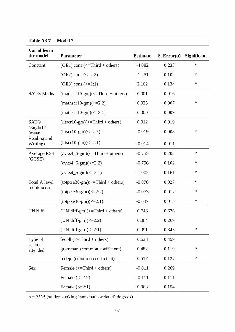
67

Table A3.7 Model 7

Variables in



(OE2) cons.(<=2:2) -1.251 0.102 *

(OE3) cons.(<=2:1) 2.162 0.134 *


(mathscr10-gm)(<=2:2) 0.025 0.007 *

(mathscr10-gm)(<=2:1) 0.000 0.009

SAT®

‘English’

(mean

Reading and

Writing)


(litscr10-gm)(<=2:2) -0.019 0.008 *

(litscr10-gm)(<=2:1) -0.014 0.011

Average KS4

(GCSE)


(avks4_6-gm)(<=2:2) -0.796 0.102 *

(avks4_6-gm)(<=2:1) -1.002 0.161 *

Total A level

points score


(totptse30-gm)(<=2:2) -0.073 0.012 *

(totptse30-gm)(<=2:1) -0.037 0.015 *


(UNIdiff-gm)(<=2:2) 0.084 0.269

(UNIdiff-gm)(<=2:1) 0.991 0.345 *

Type of

school

attended




Sex Female (<=Third + others) -0.011 0.269

Female (<=2:2) -0.111 0.111

Female (<=2:1) 0.068 0.154

n = 2335 (students taking ‘non-maths-related’ degrees)

68

Table A3.8 Model 8

Variables in



(OE2) cons.(<=2:2) -1.052 0.068 *

(OE3) cons.(<=2:1) 2.038 0.081 *

Maths KS4 /

GCSE score

(ks4maths)(<=Third + others) -0.174 0.084 *

(ks4maths)(<=2:2) -0.228 0.040 *

(ks4maths)(<=2:1) -0.344 0.071 *

UNIdiff

(UNIdiff-gm)(<=Third + others) -0.564 0.419

(UNIdiff-gm)(<=2:2) -1.549 0.210 *

(UNIdiff-gm)(<=2:1) -0.562 0.267 *

Type of school

attended


grammar. (common coefficient) 0.160 0.102


n = 2625

69

Table A3.9 Model 9

Variables in



(OE2) cons.(<=2:2) -1.022 0.068 *

(OE3) cons.(<=2:1) 2.065 0.082 *

SAT® Maths

(mathscr10-gm)(<=Third + others) -0.013 0.011

(mathscr10-gm)(<=2:2) -0.007 0.005

(mathscr10-gm)(<=2:1) -0.040 0.007 *

UNIdiff


(UNIdiff-gm)(<=2:2) -1.824 0.216 *

(UNIdiff-gm)(<=2:1) -0.461 0.264

Type of

school

attended




n = 2625

70

Table A3.10 Model 10

Variables in



(OE2) cons.(<=2:2) -1.052 0.068 *

(OE3) cons.(<=2:1) 2.055 0.082 *

SAT® Maths

(mathscr10-gm)(<=Third + others) -0.006 0.012

(mathscr10-gm)(<=2:2) 0.009 0.005

(mathscr10-gm)(<=2:1) -0.032 0.008 *

Maths KS4 /

GCSE score

(ks4maths)(<=Third + others) -0.137 0.098

(ks4maths)(<=2:2) -0.266 0.045 *

(ks4maths)(<=2:1) -0.173 0.075 *

UNIdiff


(UNIdiff-gm)(<=2:2) -1.620 0.217 *

(UNIdiff-gm)(<=2:1) -0.326 0.267

Type of

school

attended




n = 2625

71


Variables in



(OE2) cons.(<=2:2) -1.144 0.070 *

(OE3) cons.(<=2:1) 1.994 0.081 *

English KS4 /

GCSE score

(ks4eng)(<=Third + others) -0.636 0.106 *

(ks4eng)(<=2:2) -0.643 0.054 *

(ks4eng)(<=2:1) -0.434 0.077 *

UNIdiff

(UNIdiff-gm)(<=Third + others) 0.057 0.420

(UNIdiff-gm)(<=2:2) -1.048 0.212 *

(UNIdiff-gm)(<=2:1) -0.550 0.261 *

Type of school

attended




n = 2625

72


Variables in



(OE2) cons.(<=2:2) -1.052 0.067 *

(OE3) cons.(<=2:1) 2.037 0.080 *

SAT® Reading

(readscr10)(<=Third + others) -0.019 0.011

(readscr10)(<=2:2) -0.031 0.005 *

(readscr10)(<=2:1) -0.036 0.007 *

UNIdiff


(UNIdiff-gm)(<=2:2) -1.484 0.208 *

(UNIdiff-gm)(<=2:1) -0.576 0.256 *

Type of school

attended




n = 2625

73


Variables in



(OE2) cons.(<=2:2) -1.150 0.069 *

(OE3) cons.(<=2:1) 2.001 0.080 *

SAT® Reading

(readscr10)(<=Third + others) 0.005 0.012

(readscr10)(<=2:2) -0.011 0.005 *

(readscr10)(<=2:1) -0.026 0.007 *

English KS4 /

GCSE score


(ks4eng)(<=2:2) -0.596 0.059 *

(ks4eng)(<=2:1) -0.314 0.083 *

UNIdiff


(UNIdiff-gm)(<=2:2) -0.944 0.211 *

(UNIdiff-gm)(<=2:1) -0.312 0.264

Type of school

attended


grammar (common coefficient) 0.272 0.103 *


n = 2625

74


Variables in



(OE2) cons.(<=2:2) -1.144 0.070 *

(OE3) cons.(<=2:1) 1.994 0.081 *

English KS4 /

GCSE score (ks4eng)(<=Third + others) -0.636 0.106 *

(ks4eng)(<=2:2) -0.643 0.054 *

(ks4eng)(<=2:1) -0.434 0.077 *

UNIdiff


(UNIdiff-gm)(<=2:2) -1.048 0.212 *

(UNIdiff-gm)(<=2:1) -0.550 0.261 *

Type of school

attended fecoll.(<=Third + others) 0.731 0.389



n = 2625

75


Variables in



(OE2) cons.(<=2:2) -1.078 0.070 *

(OE3) cons.(<=2:1) 2.016 0.081 *

SAT® Writing

(writescr10)(<=Third + others) -0.035 0.015 *

(writescr10)(<=2:2) -0.050 0.007 *

(writescr10)(<=2:1) -0.045 0.009 *

UNIdiff


(UNIdiff-gm)(<=2:2) -1.388 0.214 *

(UNIdiff-gm)(<=2:1) -0.614 0.264 *

Type of school

attended




n = 2625

76


Variables in



(OE2) cons.(<=2:2) -1.156 0.070 *

(OE3) cons.(<=2:1) 1.992 0.081 *

SAT® Writing

(writescr10)(<=Third + others) 0.007 0.017

(writescr10)(<=2:2) -0.018 0.007 *

(writescr10)(<=2:1) -0.028 0.010 *

English KS4 /

GCSE score


(ks4eng)(<=2:2) -0.579 0.061 *

(ks4eng)(<=2:1) -0.329 0.086 *

UNIdiff


(UNIdiff-gm)(<=2:2) -0.937 0.214 *

(UNIdiff-gm)(<=2:1) -0.358 0.269

Type of school

attended




n = 2625

77


Variables in the

model Parameter Estimate S. Error(u) Significant


(OE2) cons.(<=2:2) -1.216 0.070 *

(OE3) cons.(<=2:1) 2.133 0.086 *


(mathscr10-gm)(<=2:2) 0.030 0.005 *

(mathscr10-gm)(<=2:1) -0.014 0.008

SAT® ‘English’

(mean Reading

and Writing)


(litscr10-gm)(<=2:2) -0.018 0.007 *

(litscr10-gm)(<=2:1) -0.003 0.010

Average KS4

(GCSE)

(avks4_6-gm)(<=Third + others) 0.093 0.290

(avks4_6-gm)(<=2:2) -0.072 0.249

(avks4_6-gm)(<=2:1) -0.128 0.279

Total A level

points score


(totptse30-gm)(<=2:2) -0.070 0.010 *

(totptse30-gm)(<=2:1) -0.044 0.013 *


(UNIdiff-gm)(<=2:2) 0.297 0.242

(UNIdiff-gm)(<=2:1) 1.241 0.307 *

Type of school

attended




GCSE (pupil) /

HE progression

rate

K4prog.(common coefficient) -0.010 0.003 *

n = 2754

78


Variables in



(OE2) cons.(<=2:2) -1.899 0.118 *

(OE3) cons.(<=2:1) 1.715 0.119 *


(mathscr1-gm)(<=2:2) 0.051 0.008 *

(mathscr1-gm)(<=2:1) -0.018 0.010

SAT®

‘English’

(mean Reading

and Writing)


(litscr10-gm)(<=2:2) -0.024 0.011 *

(litscr10-gm)(<=2:1) -0.030 0.013 *

Average KS4

(GCSE)


(avks4_6-gm)(<=2:2) -1.156 0.146 *

(avks4_6-gm)(<=2:1) -1.130 0.198 *

Total A level

points score


(totptse30-gm)(<=2:2) -0.079 0.016 *

(totptse30-gm)(<=2:1) -0.013 0.016


(UNIdiff-gm)(<=2:2) 0.300 0.541

(UNIdiff-gm)(<=2:1) 1.961 0.598 *

Type of school

attended




n = 1381 (graduates of Sutton Trust ‘Top 30’ universities)

79


Variables in



(OE2) cons.(<=2:2) -0.695 0.079 *

(OE3) cons.(<=2:1) 2.478 0.126 *


(mathscr1-gm)(<=2:2) 0.012 0.007

(mathscr1-gm)(<=2:1) -0.021 0.012

SAT®

‘English’

(mean Reading

and Writing)


(litscr10-gm)(<=2:2) -0.008 0.009

(litscr10-gm)(<=2:1) 0.035 0.016 *

Average KS4

(GCSE)

(avks4_6-gm)(<=Third + others) -0.371 0.228

(avks4_6-gm)(<=2:2) -0.570 0.116 *

(avks4_6-gm)(<=2:1) -0.590 0.203 *

Total A level

points score


(totptse30-gm)(<=2:2) -0.074 0.014 *

(totptse30-gm)(<=2:1) -0.103 0.022 *


(UNIdiff-gm)(<=2:2) -1.283 0.798

(UNIdiff-gm)(<=2:1) 0.482 1.014

Type of school

attended




n = 1373 (graduates of other universities excluding Sutton Trust ‘Top 30’)

80

Appendix 4: Measuring the goodness of fit of ordered categorical models

In a linear regression model, we can calculate the R2 statistic as a measure of the goodness of

fit of the model. The value is always between zero and one, and can be interpreted as the

proportion of the variation in outcomes which is explained by the model. However, for

categorical models it is not possible to calculate an R2 statistic (intuitively, the difficulty

becomes clear when one considers what could be meant by the ‘proportion of variation in

outcomes’ for a categorical outcome).

Instead a pseudo-R2 such as McFadden’s R

2 is used, which, whilst being calculated in a very

different manner to the normal R2, is analogous to it. McFadden’s R

2 is a measure of the

goodness of fit of the model and takes values between zero and one; however it cannot be

interpreted as the proportion of variation explained by the model. A rule of thumb is that

values between 0.2 and 0.4 indicate a very good model fit.26

McFadden’s R2 is calculated by comparing the log-likelihood

27 of the model in question with

that of a ‘base’ model containing no explanatory variables. The greater the improvement in

log-likelihood achieved through inclusion of explanatory variables, the higher the value of

McFadden’s R2. Note that because of its reference to a base model, values should only be

compared across models where they share a common base (i.e. they make use of the same

outcome variables and include the same set of students). For example, this means that values

should not be compared between the maths subject and non-maths subject models (models 6

and 7).

26

See http://www.soziologie.uni-halle.de/langer/pdf/papers/rc33langer.pdf 27

The likelihood function captures the probability that a given set of outcomes are observed for a particular

model of interest. The log-likelihood is calculated simply by taking the logarithm of this.

http://www.soziologie.uni-halle.de/langer/pdf/papers/rc33langer.pdf

81

Table A4.1 McFadden's R2 for the ordered categorical models

Model

McFadden's R2

Base model (constants/thresholds & hierarchy only): N =

2754

1

Core model: SAT® English, SAT® Maths, UNIdiff and

school type 0.12

2 Core model + average KS4 points + average A level points 0.74

3 Core model + average KS4 points + total A levels points 0.64

4 Core model + average KS4 points 0.57

5 Core model + average KS4 points + total A levels points+

sex + ethnicity 0.53

6 Model 3 + sex for students studying maths subjects only 0.35

Base case for model 6 (N = 419)

7 Model 3 + sex for students studying non-maths subjects only 0.94

Base case for model 7 (N = 2336)

8 KS4 maths + UNIdiff + school type 0.00

9 SAT® Maths + UNIdiff + school type 0.01

10 KS4 maths + SAT® Maths + UNIdiff + school type 0.06

11 KS4 English + UNIdiff + school type 0.29

12 SAT® Reading + UNIdiff + school type 0.02

13 KS4 English + SAT® Reading + UNIdiff + school type 0.33

14 KS4 English + UNIdiff + school type 0.29

15 SAT® Writing + UNIdiff + school type 0.06

16 KS4 English + SAT® Writing + UNIdiff + school type 0.32

Base case for models 8-16 (N = 2625)

17 Model 3 + interactions 0.66

18 Model 3 for Sutton Trust Top 30 students only 0.94

Base case for above (N = 419)

19 Model 3 for non-Sutton Trust university students only 0.42

Base case for above (N = 419)