CONSTRUCT VALIDITY OF THE GRE APTITUDE TEST

ACROSS POPULATIONS--AN EMPIRICAL

CONFIRMATORY STUDY

D. A. Rock C. Werts J. Grandy

GRE Board Professional Report GREB No. 78-1P ETS Research Report 81-37

June 1982

This report presents the findings of a research project funded by and carried out under the auspices of the Graduate Record Examinations Board.

GRE BOARD KESEARCH REPORTS FOR GENERAL AUDIENCE

Altman, R. A. and Wallmark, M. M. A Summary of Data from the Graduate Programs and Admissions Manual. GREB N;. 74-lR, January 1975.

Baird, L. L. An Inventory of Accomplishments. GREB No. 1979.

Documented 77-3R, June

Baird, L. L. Cooperative Student Survey (The Graduates [$2.50 each], and Careers and Curricula). GREB No. 7@4R, March 1973.

Baird, L. L. The Relationship Between Ratings of Graduate Departments and Faculty Publication Rates. GREB No. 77-2aR, November 1980.

Baird, L. L. and Knapp, J. E. The Inventory of Documented Accomplishments for Graduate Admissions: Results of a Field Trial Study of Its Reliability, Short-Term Correlates, and Evaluation. GREB NO. 78-3~~ August 1981.

Burns, R. L. Graduate Admissions and Fellowship Selection Policies and Procedures (Part I and II). GREB No. 69-5R, July 1970.

Centra, J. A. How Universities Evaluate Faculty Performance: A Survey of Department Heads. GREB No. 75-5bR, July 1977. ($1.50 each)

Centra, J. A. Women, Men and the Doctorate. GREB No. 71-lOR, September 1974. ($3.50 each)

Clark, M. J. The Assessment of Quality in Ph.D. Programs: A Preliminary Report on Judgments by Graduate Deans. GREB No. 72-7aR, October 1974.,

Clark, M. J. Program Review Practices of University Departments. GREB No. 75-5aR, July 1977. ($1.00 each)

DeVore, R. and McPeek, M. A Study of the Content of Three GRE Advanced Tests. GREB No. 78-4R, March 1982.

Donlon, T. F. Annotated Bibliography of Test Speededness. GREB No. 76-9R, June 1979.

Flaugher, R. L. The New Definitions of Test Fairness In Selection: Developments and Implications. GREB No. 72-4R, May 1974.

Fortna, R. 0. Annotated Bibliography of the Graduate Record Examinations. July 1979.

Frederiksen, N. and Ward, W. C. Measures for the Study of Creativity in Scientific Problem-Solving. May 1978.

Hartnett, R. T. Sex Differences in the Environments of Graduate Students and Faculty. GREB No. 77-2bR, March 1981.

Hartnett, R. T. The Information Needs of Prospective Graduate Students. GREB NO. 77-8R, October 1979.

Hartnett, R. T. and Willingham, We W. The Criterion Problem: What Measure of Success in Graduate Education? GREB No. 77-4R, March 1979.

Knapp, J. and Hamilton, I. B. The Effect of Nonstandard Undergraduate Assessment and Reporting Practices on the Graduate School Admissions Process. GREB No. 76-14R, July 1978.

Lannholm, G. V. and Parry, M. E. Programs for Disadvantaged Students in Graduate Schools. GREB No. 69-IR, January 1970.

Miller, R. and Wild, C. L. Restructuring the Graduate Record Examinations Aptitude Test. GRE Board Technical Report, June 1979.

Reilly, R. R. Critical Incidents of Graduate Student Performance. GREB No. 7O-5R, June 1974.

Rock, D., Werts, C. An Analysis of Time Related Score Increments and/or Decre- ments for GRE Repeaters across Ability and Sex Groups. GREB No. 77-9R, April 1979.

Kock, D. A. The Prediction of Doctorate Attainment in Psychology, Mathematics and Chemistry. GREB No. 69-6aR, June 1974.

Schrader, W. B. GRE Scores as Predictors of Career Achievement in History. GREB No. 76-lbR, November 1980.

Schrader, W. B. Admissions Test Scores as Predictors of Career Achievement in Psychology. GREB No. 76-laR, September 1978.

Swinton, S. S. and Powers, D. E. A Study of the Effects of Special Preparation on GRE Analytical Scores and Item Types. GREB No. 78-2R, January 1982.

Wild, C. L. Summary of Research on Restructuring the Graduate Record Examinations Aptitude Test. February 1979.

Wild, C. L. and Durso, R. Effect of Increased Test-Taking Time on Test Scores by Ethnic Group, Age, and Sex. GREB No. 76-6R, June 1979.

Wilson, K. M. The GRE Cooperative Validity Studies Project. GREB No. 75-8R, June 1979.

Wiltsey, R. G. Doctoral Use of Foreign Languages: A Survey. GREB No. 70-14R, 1972. (Highlights $1.00, Part I $2.Oc), Part II $1.50).

Witkin, H. A.; Moore, C. A.; Oltman, P. K.; Goodenough, D. F.; Friedman, F.; and Owen, D. R. A Longitudinal Study of the Role of Cognitive Styles in Academic Evolution During the College Years. GREB No. 76-lOR, February 1977 ($5.OQ each).

CONSTRUCT VALIDITY OF THE GRE APTITUDE TEST ACROSS POPULATIONS--

AN EMPIRICAL CONFIRMATORY STUDY

D. A. Rock

C. Werts

J. Grandy

GRE Board Professional Report GREB No. 78-1P

June 1982

Copyright@1982 by Educational Testing Service. All rights reserved.

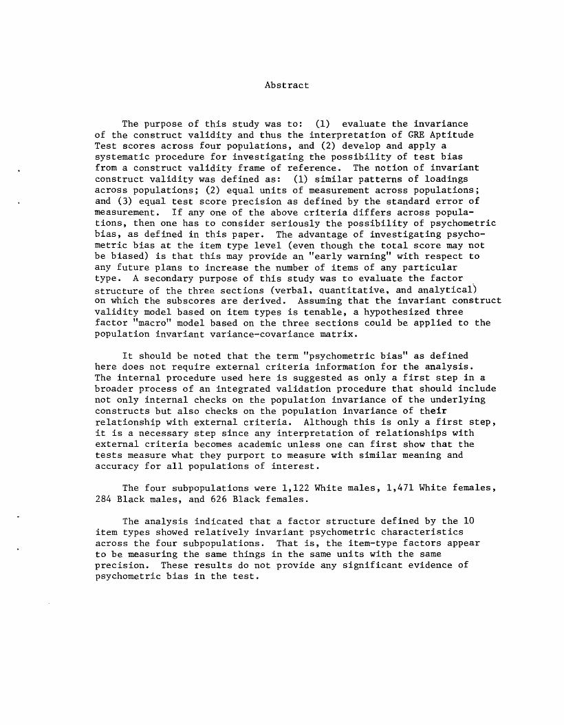
Abstract

The purpose of this study was to: (1) evaluate the invariance of the construct validity and thus the interpretation of GRE Aptitude Test scores across four populations, and (2) develop and apply a systematic procedure for investigating the possibility of test bias from a construct validity frame of reference. The notion of invariant construct validity was defined as: (1) similar patterns of loadings across populations; (2) equal units of measurement across populations; and (3) equal test score precision as defined by the standard error of measurement. Tf any one of the above criteria differs across popula- tions, then one has to consider seriously the possibility of psychometric bias, as defined in this paper. The advantage of investigating psycho- metric bias at the item type level (even though the total score may not be biased) is that this may provide an "early warning" with respect to any future plans to increase the number of items of any particular type* A secondary purpose of this study was to evaluate the factor structure of the three sections (verbal, quantitative, and analytical) on which the subscores are derived. Assuming that the invariant construct validity model based on item types is tenable, a hypothesized three factor "macro" model based on the three sections could be applied to the population invariant variance-covariance matrix.

It should be noted that the term "psychometric bias" as defined here does not require external criteria information for the analysis. The internal procedure used here is suggested as only a first step in a broader process of an integrated validation procedure that should include not only internal checks on the population invariance of the underlying constructs but also checks on the population invariance of their relationship with external criteria. Although this is only a first step, it is a necessary step since any interpretation of relationships with external criteria becomes academic unless one can first show that the tests measure what they purport to measure with similar meaning and accuracy for all populations of interest.

The four subpopulations were 1,122 White males, 1,471 White females, 284 Black males, and 626 Black females.

The analysis indicated that a factor structure defined by the 10 item types showed relatively invariant psychometric characteristics across the four subpopulations. That is, the item-type factors appear to be measuring the same things in the same units with the same precision. These results do not provide any significant evidence of psychometric bias in the test.

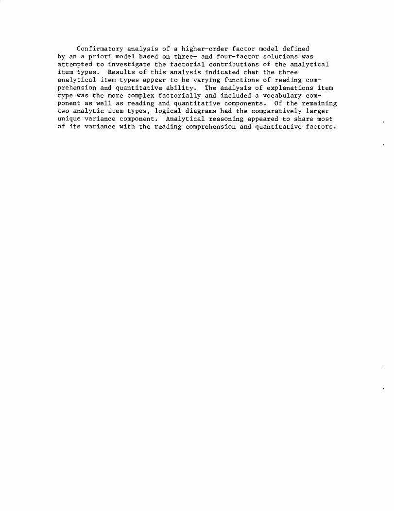
Confirmatory analysis of a higher-order factor model defined by an a priori model based on three- and four-factor solutions was attempted to investigate the factorial contributions of the analytical item types. Results of this analysis indicated that the three analytical item types appear to be varying functions of reading com- prehension and quantitative ability. The analysis of explanations item type was the more complex factorially and included a vocabulary com- ponent as well as reading and quantitative components. Of the remaining two analytic item types, logical diagrams had the comparatively larger unique variance component. Analytical reasoning appeared to share most of its variance with the reading comprehension and quantitative factors.

Construct Validity of the GRE Aptitude Test

Across Populations-- An Empirical Confirmatory Study

D. A. Rock, C. Werts, and J. Grandy

Introduction

Construct validation is the basic prerequisite to proper interpretation

of a test score. Any time an educator asks "But what does the instru-

ment really measure?" information on construct validity is being

requested (e.g., see Cronbach, 1971). Construct validation is the

process of marshalling evidence of relationships with other variables

to support the inference that an observed test score has a particular

meaning; for example, that it is a valid measure of developed verbal or

mathematical ability. Implicit in this definition is the presence of

an a priori theory or model that in turn generates predictions about

expected correlational patterns among measures of the construct of

interest as well as with measures of other relevant constructs.

The presence of empirical findings that are consistent with the

a priori model furnishes support for the construct validity of the

measuring instrument. Empirical findings that are at variance with

the a priori model either cast doubt on interpretation of the test

score or at best limit its interpretation (Campbell 6 Fiske, 1959).

Operationally, this study attempts to accomplish two goals.

First, it investigates the stability of item type factor inter-

relationships as well as thier psychometric characteristics across

-2-

Black male, Black female, White male, and White female populations.

Secondly, it examines the convergent and discriminant validity of

the verbal, quantitative, and analytical ability sections of the GRE

Aptitude Test. The term convergent validity simply means that the

item types that are assumed to be measures of a hypothetical construct

such as analytical ability should demonstrate proportionately higher

interrelationships among themselves than with measures of other

constructs such as verbal or quantitative ability. The term dis-

criminant validity suggests that hypothetical constructs such as

verbal, quantitative, and analytical ability are more usefully

interpreted if they can be shown empirically to be measuring different

things.

Recent procedures in maximum likelihood confirmatory factor

analysis (SBrbom, 1974) allow researchers to: (1) test for "goodness

of fit" an a priori factor pattern model based on item types; (2) es-

timate and test equality of units of measurement for equivalent item-

type sections; (3) estimate and test the reliability or accuracy with

which each of the item-type factors are measured; and (4) test the

invariance of the item-type factors across populations. That is, does

the test measure the same things in the same units with equal precision

for all subpopulations? If the data do not confirm that the test is

measuring the same things in the same units across subpopulations, then

the test score interpretations must be called into question.

The GRE verbal, quantitative, and analytical ability sections can

-3-

be subdivided into 10 subsections based on item-type classifications.

If it can be shown at this relatively micro level (i.e., the item-

type level) that the 10 item-type factors are measuring the same things

with the same accuracy across all populations, then we can use the

maximum likelihood (MLH) estimate of the population invariant variance-

covariance matrix resulting from the best fitting factor model to

investigate the relationships between item types and the developed

abilities they purport to measure. That is, using the MLH estimate of

the population invariant variance-covariance matrix, one can confirm

or disconfirm an a priori model in which the four verbal item types

define a verbal factor, the three quantitative item types define a

quantitative factor, and an analytical factor is defined by its three

respective item types. Such an analysis will confirm the usefulness

of maintaining these separate scores as well as provide information on

the psychometric contribution of the respective item types to their

underlying factor or construct.

Testing the Invariance of Psychometric Characteristics Across Populations

The first step is to examine the comparability of the pattern of

loadings across populations. Assuming that one finds empirical evidence

for the similarity of the pattern of factor loadings on the hypothesized

item factors in each population, then one can ask whether the scale

units for the reading factor, analogy factor, etc. are the same across

populations. Being tested here is whether the corresponding factor

loadings are the same across populations when the factors are given

the observed units of one of thier indicator variables. That is, if we

hypothesize that a given factor, e. g., the reading comprehension

factor, can be defined by two split-halved scores from the reading

comprehension section, and the factor is given the raw score units

of the odd-item half, then if the model is correct, the factor

loadings for the even and odd item subtest scores should be equiva-

lent both within and across populations. The important point here,

however, is not so much whether the two reading comprehension split

halves are tau equivalent within each population (i.e., have equivalent

odd and even factor loadings in raw score units) but whether they

maintain their proportionality ratio across the populations.

If the scale units are found to be different in one or more

populations, one must conclude that the interpretation of the observed

scores may not be equivalent across populations. Such a situation is

the internal or psychometric counterpart of the "test bias" definition

that argues that a test is biased against one group or another if the

slopes of the regressions of an external criterion on the test are not

the same (e.g., see Cleary, 1968). However, in this case we are

comparing the slope of the observed scores on the true scores across

groups or populations. As JEreskog (1971) points out, if the variables

that define each factor can be shown to be at least congeneric (i.e.,

measures of the same thing as indicated by similar patterns of salient

loadings), then the maximum likelihood estimates of the raw score

factor loadings are the regressions of the observed scores on their

"true" scores. If the corresponding raw score factor loadings are

-5-

equal, then we would expect that the true score difference corres-

ponding to a particular observed score difference would be uniform

across populations. The reader should note here that we are

referring to the maximum likelihood "raw score" factor loading esti-

mated from the variance-covariance matrix and not the traditional

standardized loadings derived from least squares solutions applied to

a correlation matrix. Such standardized solutions can neither estimate

nor test the equivalence of measurement units across populations.

In addition to gathering empirical evidence that a test is

measuring the same things in the same units, one should also demonstrate

that the test is measuring with the same precision across all populations.

That is, a third, albeit less serious, indicator of possible psychometric

bias is the finding of the nonequivalence across populations of the

precision with which each factor or construct is measured. Specifically,

are the standard errors of measurement of the factors underlying the

test the same across all populations? Tests of the equivalence of the

standard errors of measurement are only meaningful, however, if we have

first shown that we are measuring the same things in the same scale

units. The standard error of measurement is preferable to the tradi-

tional reliability estimates as an indicator of a test score's precision

since it is more likely to be invariant across populations that differ

with respect to the amount of variability in the trait being measured.

When one is comparing the precision of test scores across populations

characterized by differing variability with respect to the trait of

-6-

interest, the traditional reliability indices confound population

heterogeneity with measurement error (see, for example, Wiley, 1973).

The question arises, Why investigate the invariance of the

psychometric characteristics of the GRE Aptitude Test through the use

of item types rather than through the use of other categories such as

content areas? There are a number of practical and theoretical reasons

for the choice of item types rather than content areas or processes.

First, the test specifications with respect to item types are relatively

stable, both across form and time of administration. Second, the three

subscores presently used are defined by item types. Third, item types

can be thought of as different methods of measuring their respective

constructs, and previous research (Campbell & Fiske, 1959; Rock &

Werts, 1979) suggests that method factors are present and are significant

sources of variance. Fourth, since this is a confirmatory analysis whose

goal is to investigate the invariance of the psychometric properties of

the GRE Aptitude Test, an objective means for conveniently classifying

items to form an a priori factor model is necessary.

-7-

Purpose

The primary purpose of this study is to evaluate the invariance of

the construct validity of the GRE Aptitude Test and thus interpreta-

tion of the test scores across four populations. The subpopulations

we will be concerned with here are White males, White females, Black

males, and Black females. The notion of invariant construct validity

is defined as (1) similar patterns of loadings across populations,

(2) equal units of measurement across populations, and (3) equal test

score precision as defined by the standard error of measurement. If

any one of these criteria differs across populations, then one has to

consider seriously the possibility of psychometric bias, as defined in

this paper. The advantage of investigating psychometric bias at the

item-type level (even though the total score may not be biased) is

that this may provide helpful information with respect to any test

development decisions concerning item-type representation in the total

test specifications. A secondary purpose of this study is to evaluate

the factor structure of the three sections, (verbal, quantitative, and

analytical ability) on which separate scores are derived. Assuming

that the invariant construct validity model based on item types is

tenable, this hypothesized three-factor "macro" model will be carried

out on the maximum likelihood estimate of the population invarient

variance-covariance matrix.

Sample

Scores were gathered for a total of 3,503 social science majors who

were also American citizens and were taking the GRE Aptitude Test for

-8-

the first time. These individuals were part of the September 1978

test administration. The total sample was further divided into four

subpopulations: 1,122 White males, 1,471 White females, 284 Black

males, and 626 Black females. These four subpopulations were used

in the subsequent comparisons of the factor models. The matching

on major field, etc. was carried out in an effort to minimize the

possibility of confounding other background factors with the effects

of racial and sex group memberships.

Method

Sgrbom and Jgreskog's (1976) program for confirmatory factor analysis

across populations, COFAMM, was used to test the various explicit

assumptions about the invariance of the construct validity of the

GRE Aptitude Test across populations.

COFAMivl assumes that a factor analysis model holds in each of the

g populations under study. If x is defined as the vector of the -&

p observed measures in group g, then x can be accounted for by k -g

common factors (f ) and p unique factors (z >. The model in -g -g

each population is:

3 = iig + Yg + = (1) 6 -g

where v is a p x 1 vector of location parameters and A -g

_g a p x k matrix of

factor loadings. It is assumed that z and f -g -g

are uncorrelated, the

expectation of z = 0, and the expectation of f = B -g - -g -g'

where0 isakx -g

1 parameter vector.

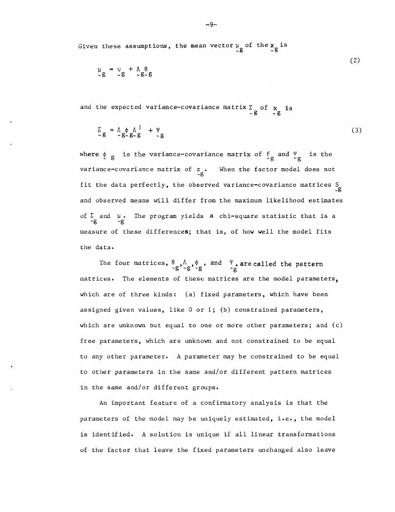
Given these assumptions, the mean vector u of thexgis ug

(2) F-l v +A8 ,g = wg -g-g

and the expected variance-covariance matrix c of x is -g -g

F: -I3

=nc$n’ +Y -g-g-g -g

where 1 g is the variance-covariance matrix of f and v is the -g -g

variance-covariance matrix of 2 . When the factor model does not -g

fit the data perfectly, the observed variance-covariance matrices S -g

and observed means will differ from the maximum likelihood estimates

of C and P . The program yields a chi-square statistic that is a -g -g

measure of these differences; that is, of how well the model fits

the data.

The four matrices, 8 ,A ,$ 9 and y,arecalled the pattern -g -g -g -g

matrices. The elements of these matrices are the model parameters,

which are of three kinds: (a) fixed parameters, which have been

assigned given values, like 0 or 1; (b) constrained parameters,

which are unknown but equal to one or more other parameters; and (c)

free parameters, which are unknown and not constrained to be equal

to any other parameter. A parameter may be constrained to be equal

to other parameters in the same and/or different pattern matrices

in the same and/or different groups.

An important feature of a confirmatory analysis is that the

parameters of the model may be uniquely estimated, i.e., the model

is identified. A solution is unique if all linear transformations

of the factor that leave the fixed parameters unchanged also leave

(3)

-lO-

the free parameters unchanged. It is difficult in general to give

useful conditions that are sufficient for identification. However,

at one point in the program the information matrix for the unknown

parameters is computed. If this matrix is positive definite, it is

almost certain that the model is identified. If this matrix is not

positive definite, the program prints a message to this effect,

specifying which parameter is probably not identified.

In all succeeding tests of these data the models are over-

identified, yielding not only unique solutions but sufficient degrees

of freedom for a statistical test of "goodness of fit." If the model

is identified, as in these examples, standard errors for all the

unknown parameter estimates are also provided by the program.

Results and Discussion

Tests of the 10 Factor Item-Type Model

The factor pattern of the GRE Aptitude Test is a special case of

equation (1) with the number of variables equal to 20 and the number

of hypothesized factors equal to 10. The factor pattern is defined

by 10 item-type factors, each of which is identified by two observed

variables. The two observed indicators of each factor are scores

on odd-even halves f or each item type yielding a total of 20 scar es--

two scores defining each item-type factor. In terms of equation w the 10 item-type factors generate the constrained loading pattern

shown in Figure 1.

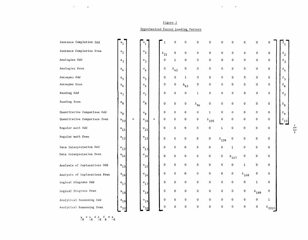
Figure 1

Hypothesized Factor Loading Pattern

Sentence Completion Odd

Sentence Completion Even

Analogies Odd

Analogies Even

Antonyms Odd

Antonyms Even

Reading Odd

Reading Even

Quantitative Comparison Odd

Quantitative Comparison Even

Regular math Odd

Regular math Even

Data Interpretation Odd

Data Interpretation Even

Analysis of Explanations Odd

Analysis of Explanations Even

Logical Diagrams Odd

Logical Diagrams Even

Analytical Reasoning Odd

Analytical Reasoning Even

xg =Vg+A f +z

-g g -g

l n

x1

x5

x6

x8

x9

x1O

x11

x12

x13

x14

x15

x16

v4

v5

v6

v7

v8

v9

v10

vll

v12

v13

v14

v15

vlG

v17

vlS

v19

v2c I l

+

.l

*21

0

0

0

0

0

0

0

0

0

0

0

0

0

0

0

0

0

0 L1

0

0

1

'42

0

0

0

0

0

0

0

0

0

0

0

0

0

0

0

0

0

0

0

0

1

A63

0

0

0

0

0

0

0

0

0

0

0

0

0

0

0

0

0

0

0

0

1

'84

0

0

0

0

0

0

0

0

0

0

0

0

0

0

0

0

0

0

0

0

1

*lo5

0

0

0

0

0

0

0

0

0

0

0

0

0

0

0

0

0

0

0

0

1

'126

0

0

0

0

0

0

0

0

0

0

0

0

0

1

%47

0

0

0

0

0

0

0

0

0

0

0

0

0

0

0

0

0

0

0

0

1

0

0

0

0

0

0

0

0

0

0

0

0

0

0

0

A 168 0

0 1

0 '189

0 0

0 0

0

0

0

0

0

0

0

0

0

0

0

0

0

0

0

0

0

0

1

A2o1o c

II.

fl

f2

f3

f4

f5

f6

f7

f8

f9

f 10

-m

-12-

One factor loading in each column is fixed at unity in order

to scale each factor arbitrarily in terms of the observed units

of its lead indicator. Thus, each factor is assumed to be deter-

mined by its split-halved odd and even item subtest scores. Conse-

quently, we are testing a "pure" simple structure derived from the

original test specifications that dictate 10 "pure" item-type

factors across all populations. We have put all our constraints

in A (i.e., the 180 loadings constrained to be zero plus the 10

loadings constrained to unity) and left the 10 x 10 factor variance-

covariance matrix (+) and the 20 x 20 diagonal matrix of errors

or uniqueness to be estimated.

Since there are 210 unique observed elements in any given

sample variance-covariance matrix, S g

(g = 1, 2, . . . . 4), and we are

only estimating 55 unknown factor variance-covariances in $, 20

unknown uniquenesses in $,and 10 unknown factor loadings in A, we

have 125 degrees of freedom (210-85) for testing "goodness of fit"

within any given population. However, since we are testing the

invariance of this factor pattern across four populations,we have

4 x 125 = 500 total degrees of freedom for our test. We shall add

the additional constraint that the intercepts, v (g = 1, 2, . ...4), g

be equal across populations. This is of course a special case of

equation (1) that will become more meaningful when we constrain the

factor loadings to be equal across populations. At that point,

we shall discuss this constraint in more detail.

-13-

If the GRE 10 factor model is consistent with the data, then

the difference between the observed variance-covariance matrix (Sg)

and the constrained populations variance-covariance matrix (Zg)

is essentially a null matrix for all groups. The interpretation

would be that there are 10 item-type factors present in all popula-

tions and the respective indicators of each factor are at least

congeneric (i.e., odd and even subtest scores are measuring the same

things in all populations). Since we did not constrain corresponding

unknown nonzero factor loadings to be equal across populations, we

cannot yet make the stronger statement that the subtest scores are

not only measuring the same thing but also have the same units of

measurement.

The statistical test of the hypothesis of equivalent constrained

factor patterns and equal intercepts across populations yielded a x 2

of 375 with 530 degrees of freedom (p = .999).

A more appropriate measure of "goodness of fit" in such large

samples is the matrix of differences between corresponding elements

in each population's observed variance-covariance matrix S and the g

reproduced variance-covariance matrix (C ) conditional on the con- g

strained factor model. Unfortunately, it is not easy to interpret

these discrepancies in the case of the variance-covariance matrices.

Therefore, the within-population observed and reproduced variance-

covariance matrices were resealed as correlation matrices. The

root mean square (RMS) of these standardized residuals may be

interpreted as you would interpret the residuals when fitting a

-14-

factor model to the observed correlation matrix.

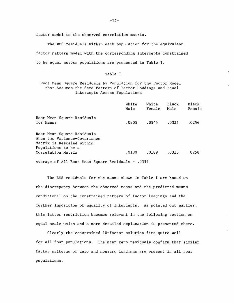
The RMS residuals within each population for the equivalent

factor pattern model with the corresponding intercepts constrained

to be equal across populations are presented in Table I.

Table I

Root Mean Square Residuals by Population for the Factor Model that Assumes the Same Pattern of Factor Loadings and Equal

Intercepts Across Populations

White White Black Black Male Female Male Female

Root Mean Square Residuals for Means .0805 .0545 .0325 .0256

Root Mean Square Residuals When the Variance-Covariance Matrix is Resealed within Populations to be a Correlation Matrix .0180 .0189 .0313 .0258

Average of All Root Mean Square Residuals = .0359

The RMS residuals for the means shown in Table I are based on

the discrepancy between the observed means and the predicted means

conditional on the constrained pattern of factor loadings and the

further imposition of equality of intercepts. As pointed out earlier,

this latter restriction becomes relevant in the following section on

equal scale units and a more detailed explanation is presented there.

Clearly the constrained lo-factor solution fits quite well

for all four populations. The near zero residuals confirm that similar

factor patterns of zero and nonzero loadings are present in all four

populations.

-15-

Equal Scaling Units Across Populations

Tf, in addition to observing the same pattern of factor loadings

in all populations, as was done in the previous step, the corresponding

factor loadings themselves are also constrained to be equal across

populations, then we can test whether the factors have the same

scale units across all populations. The hypothesis being tested may

be stated as follows: H 0: A, = I$..., ~~ conditional on a IO-

factor solution with equal intercepts across populations

against the alternative H 1: Al # A2 f,..., A4 given a lo-

factor solution and equal intercepts. Since the factor loadings

are maximum likelihood (MLH) estimates of the regressions of the

observed scores on the true scores, the constraint of equality

across populations is equivalent to a test of equality of scaling

units (when the measures are congeneric, i.e., have the same factor

loading patterns and also have the same intercepts). However,

the individual odd-even halves within populations are not

assumed to have equal scales, i.e., equal loadings or

intercepts. In this case 30 additional degrees of freedom are

gained over the previous test of 10 factoredness since a total of

30 more constraints have been added. This more restricted model led

to an increment in x2 over the previous test (i.e., the test of

-16-

similar factor patterns and the intercepts with no equality constraints

across populations on the nonzero factor loadings) of 59 with 30

degrees of freedom (p SC .OOl). Thus this hypothesis would be rejected

on purely statistical grounds. However, the large sample size almost

guarantees that very small deviations from the hypothesis would lead

to sta t istical significance. As with the previ ous test, since the 1 arge

sample size makes the usual interpretation of s tatistical tests less

meaningful, we will opt for the root mean square residuals as the

primary measure of "goodness of fit." Table II below shows the root

mean square residuals by population for this more constrained model.

There it is clear that the residuals are quite small even though they

produce a statistically significant departure from the model. It

seems reasonable to conclude that the model provides a reasonably good

fit to the data across the four subpopulations--that the item types

measure essentially the same things in essentially equal units across

all populations.

Table II

Root Mean Square Residuals by Population for the Factor Model that Assumes Equal Factor Patterns

and Equal Intercepts Across Populations

White White Black Black Male Female Male Female

Root Mean Square Residuals for Means .0523 .0626 .0363 .0350

Root Mean Square Residuals When the Variance-Covariance Matrix is Resealed within Populations to be a Correlation Matrix .0232 .0225 .0340 .0315

Average of All Root Mean Square Residuals = .0372

. -17-

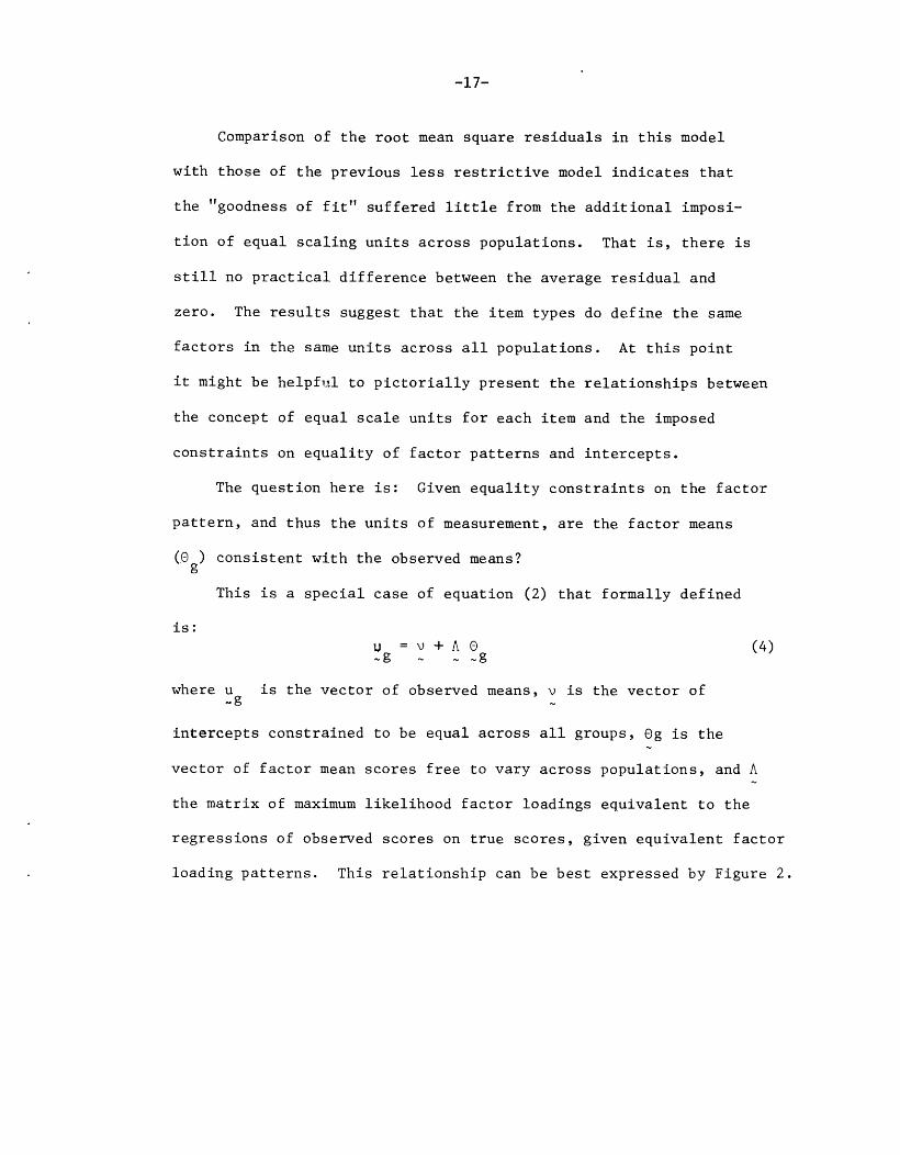
Comparison of the root mean square residuals in this model

with those of the previous less restrictive model indicates that

the "goodness of fit" suffered little from the additional imposi-

tion of equal scaling units across populations. That is, there is

still no practical difference between the average residual and

zero. The results suggest that the item types do define the same

factors in the same units across all populations. At this point

it might be helpful to pictorially present the relationships between

the concept of equal scale units for each item and the imposed

constraints on equality of factor patterns and intercepts.

The question here is: Given equality constraints on the factor

pattern, and thus the units of measurement, are the factor means

(0 g

> consistent with the observed means?

This is a special case of equation (2) that formally defined

is: =v+AO

ug .., _ -g (4)

where u -g

is the vector of observed means, v is the vector of

intercepts constrained to be equal across all groups, 8g is the

vector of factor mean s

the matrix of maximum 1

regressions of observed

loading patterns. This relationsh

cores free

ikelihood f

scores on

to vary across

actor loadings

true scores, g

ip can be best

populations, and A

equivalent to the

iven equivalent factor

expressed by Figure 2.

-18-

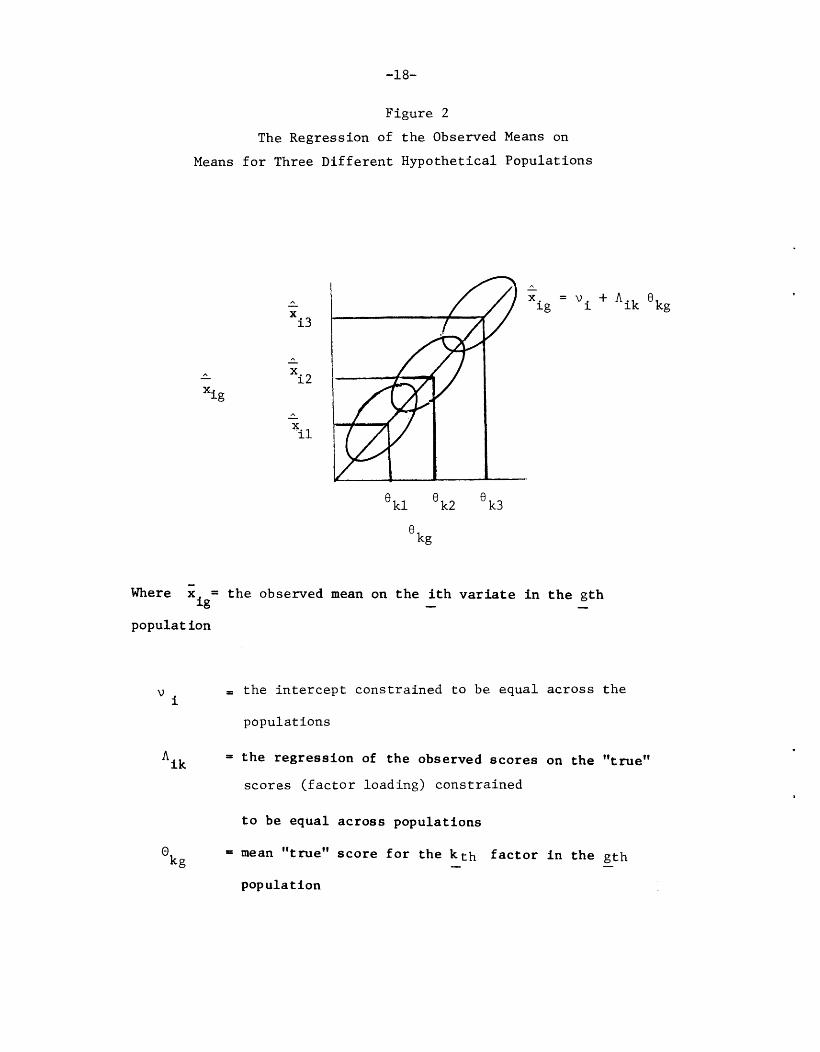
Figure 2

The Regression of the Observed Means on

Means for Three Different Hypothetical Populations

h

_;;

i3

h

x i2

h

x il

h

x ig

=v +A i ik 'kg

'kl 'k2 'k3

8 kg

Where Z ig

= the observed mean on the ith variate in the gth -

population

Vi s the intercept constrained to be equal across the

populations

A ik = the regression of the observed scores on the "true"

scores (factor loading) constrained

to be equal across populations

0 kg

= mean "true" score for the kth factor in the gth - -

population

-19-

Under the present model

all of which are assumed to

and differing only in their

may have different ability

there are, of course, four populations,

be lying along the same regression line

factor means (fj kg

>. The populations

levels as reflected by different true

score means, but the intercept and the multiplicative or scaling

parameter, A, must be the same or one must question

whether or not that particular item type is measuring in the

same scale units in all populations. When the scaling parameters

are different across populations, it is quite likely that the item

type is not measuring the same things for all populations.

Equal

The hypothesis here is that, in addition to having the same

factors measured in the same units across populations, the diagonal

elements of $ are also equal across populations. The diagonal

elements of $ are estimates of the squared standard errors of

measurement of each of the respective split-halved measures if, as

has been shown, the split-halved scores are congeneric measures with

equivalent scale units across populations. More formally, the hypothesis

being tested is: I/J, = $2 =,...,$4 conditional on equal factor loading

patterns, scaling units, and intercepts.

This restricted model assumes that all elements

of the factor model with the exception of the variance-covariance

matrix among factors (+) are equal across populations. These

additional restrictions lead to an increment in x 2

of 68 with

60 degrees of freedom (p 2 .75).

-2o-

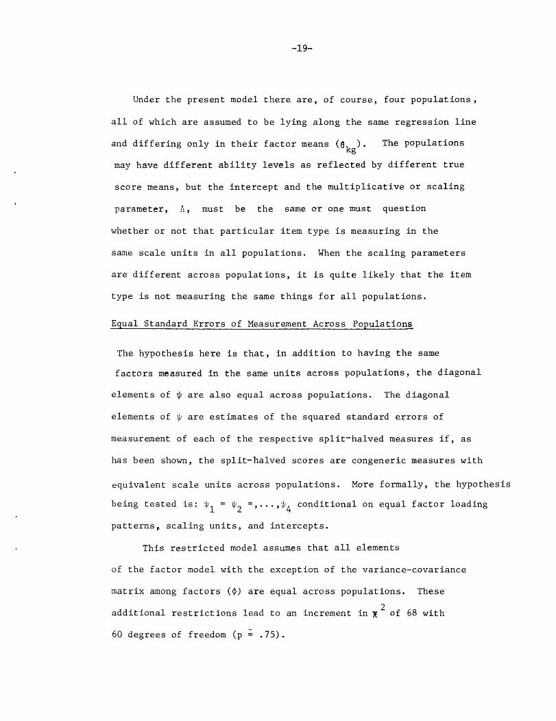
Table III below presents the root mean square residuals for

this constrained model.

Table III

Root Mean Square Residuals by Population for the Factor Model That Assumes Equal Factor Loading Patterns,

Intercepts, Units of Measurement, and Standard Error of Measurement Across Populations

White White Black Black Male Female Male Female

Root Mean Square Residuals for Means .0591 .0604 .0330

Root Mean Square Residuals When the Variance-Covariance Matrix is Resealed within Populations to be a Correlation Matrix I .0220 .0214 .0360

.0359

.0304

Average of All Root Mean Square Residuals = .0375

Clearly there is little additional "lack of fit" as measured by

the increment in residual when the standard errors of measurement

were constrained to be equal across populations. The 10 item types in

the GRE Aptitude Test appear to be measuring all populations with equal

precision.

The above three sequential tests of progressively "stronger"

models, all of which provide a reasonably good fit, suggest that the

GRE item types are measuring the same things in the same units with

the same precision for all four populations. There does not appear

to be any significant evidence of psychometric bias here. It should

be remembered that psychometric bias as defined here is only one of

many possible definitions of test bias. For other views see Darlington

(1971) and Schmidt and Hunter (1976).

-21-

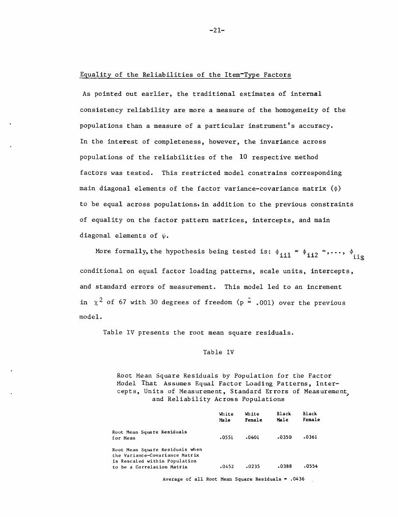
Ecrualitv of the Reliabilities of the Item-Tvne Factors

As pointed out earlier, the traditional estimates of internal

consistency reliability are more a measure of the homogeneity of the

populations than a measure of a particular instrument's accuracy.

In the interest of completeness, however, the invariance across

populations of the reliabilities of the 10 respective method

factors was tested. This restricted model constrains corresponding

main diagonal elements of the factor variance-covariance matrix ($)

to be equal across populations,in addition to the previous constraints

of equality on the factor pattern matrices, intercepts, and main

diagonal elements of $.

More formally,the hypothesis being tested is: $iil = oii2 =, . . . , @ iig

conditional on equal factor loading patterns, scale units, intercepts,

and standard errors of measurement. This model led to an increment

in x 2 of 67 with 30 degrees of freedom (p z .OOl) over the previous

model.

Table IV presents the root mean square residuals.

Table IV

Root Mean Square Residuals by Population for the Factor Model That Assumes Equal Factor Loading Patterns, Inter- cepts, Units of Measurement, Standard Errors of Measurement>

and Reliability Across Populatiorrs

White White Black Black Male Female Male Female

Root Mean Square Residuals for Mean .0551 .0601 .0350 .0361

Root Mean Square Residuals when the Variance-Covariance Matrix is Resealed within Population to be a Correlation Matrix .0452 .0235 .0388 .0554

Average of all Root Mean Square Residuals = .0436

-22-

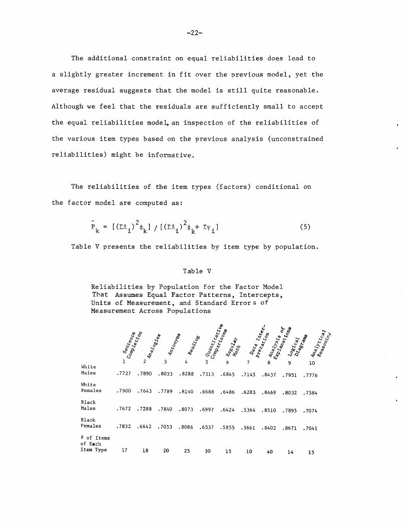
The additional constraint on equal reliabilities does lead to

a slightly greater increment in fit over the previous model, yet the

average residual suggests that the model is still quite reasonable.

Although we feel that the residuals are sufficiently small to accept

the equal reliabilities model, an inspection of the reliabilities of

the various item types based on the previous analysis (unconstrained

reliabilities) might be informative.

The reliabilities of the item types (factors) conditional on

the factor model are computed as:

(5)

Table V presents the reliabilities by item type by population.

Table V

Reliabilities by Population for the Factor Model That Assumes Equal Factor Patterns, Intercepts, Units of Measurement, and Standard Errors of Measurement Across Populations

1 2 3 4 5 6 7 8. 9 White Males .7727 .7890 .8033 .8288 .7313 .6845 ,714s .8437 .7951 .7776

White Females .7900 .7643 .7789 .8140 .6688 .6486 .6283 .8469 .8032 .7584

Black Males . 7672 .7288 .7840 .8073 .6997 .6424 .5364 .8510 a7895 .7074

Black Females .7832 .6642 .7053 .8086 .6537 .5855 .5661 .8402 .8671 .7041

I of Items of Each Item Type 17 18 20 25 30 15 10 40 14 15

Inspection of Table V suggests little in the way of consistent

patterns, although there is some tendency for scores of Blacks to

to have somewhat lower reliabilities than the corresponding scores

of Whites. Similarly, scores of White females and to somewhat

lesser extent those of Black females tend to have slightly lower

reliabilities than the scores of their male counterparts.

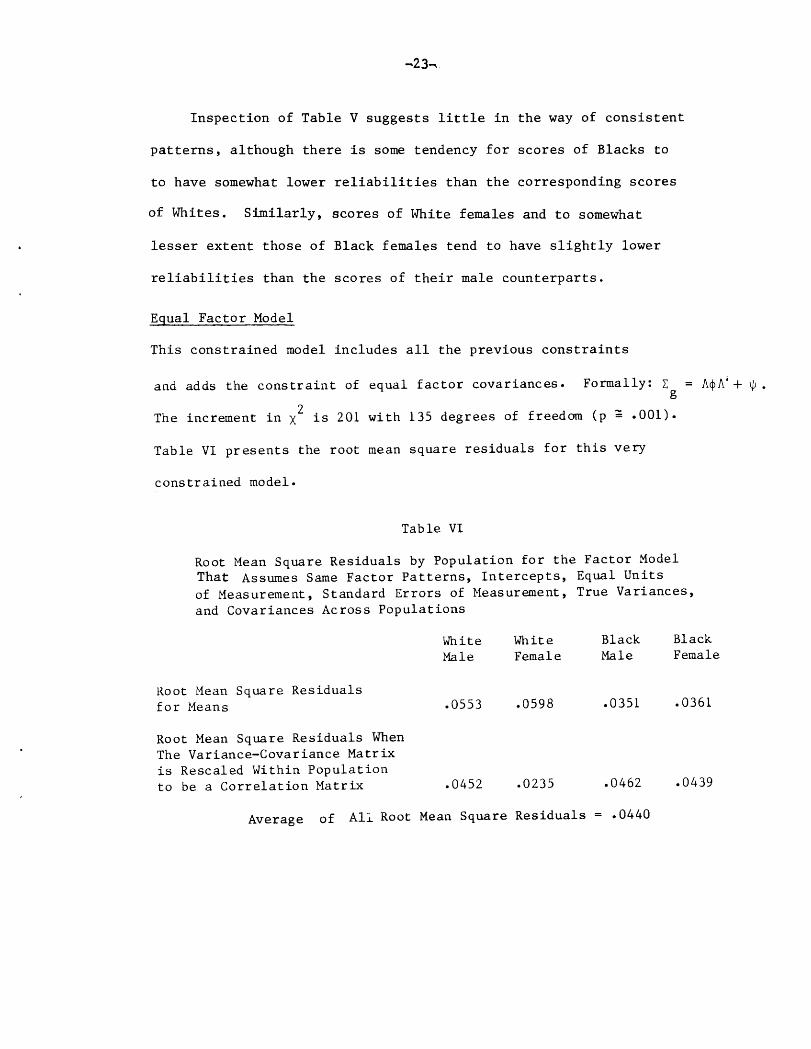
Eaual Factor Model

This constrained model includes all the previous constraints

and adds the constraint of equal factor covariances. Formally: c = @IA'+ IJ,. g

The increment in x2 is 201 with 135 degrees of freedom (p g .OOl)=

Table VI presents the roo t mean square residuals for this very

constrained model.

Table VI

Root Mean Square Residuals by Population for the Factor Model That Assumes Same Factor Patterns, Intercepts, Equal Units of Measurement, Standard Errors of Measurement, True Variances, and Covariances Across Populations

White White Black Male Female Male

Root Mean Square Residuals for Means .0553 .0598 .0351

Root Mean Square Residuals When The Variance-Covariance Matrix is Resealed Within Population to be a Correlation Matrix .0452 .0235 .0462

Average of Ali Root Mean Square Residuals = .O44O

Black Female

.0361

.0439

-26

Inspection of the residuals in Table VI supports a reasonable

fit for this model. In a certain sense this is a stronger model than

one requiring equality of the observed variance-covariance matrices

across populations since we are further imposing a specific factor structure

dictated by the original test construction specifications. The factor

loading patterns and intercorrelations among factors for this fully con-

strained model are presented in Appendices B and C.

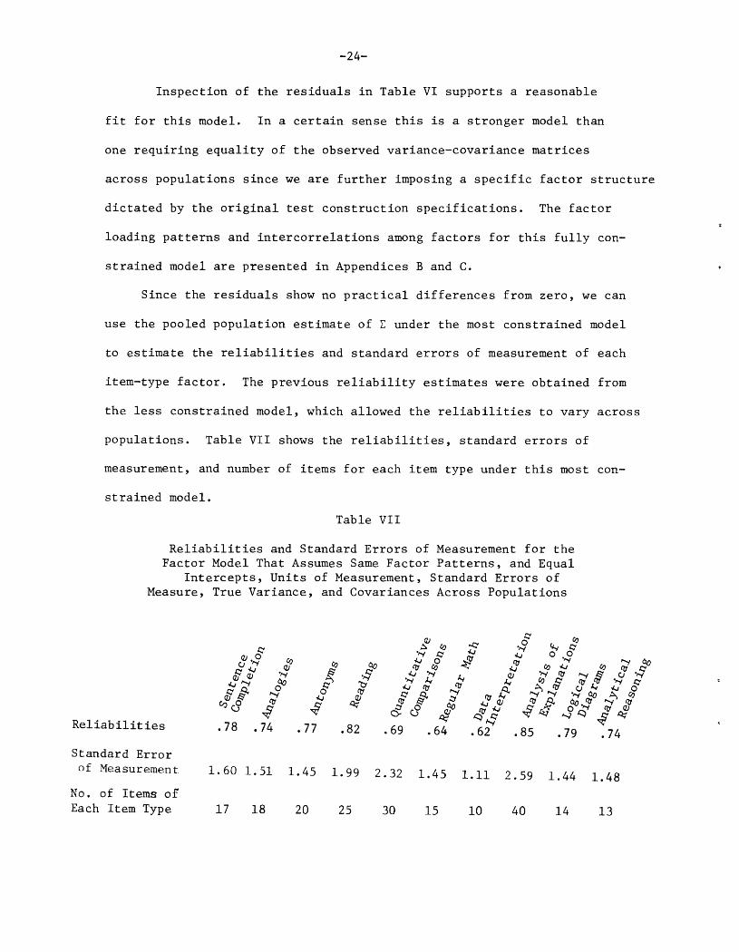
Since the residuals show no practical differences from zero, we can

use the pooled population estimate of C under the most constrained model

to estimate the reliabilities and standard errors of measurement of each

item-type factor. The previous reliability estimates were obtained from

the less constrained model, which allowed the reliabilities to vary across

populations. Table VII shows the reliabilities, standard errors of

measurement, and number of items for each item type under this most con-

strained model.

Table VII

Reliabilities and Standard Errors of Measurement for the Factor Model That Assumes Same Factor Patterns, and Equal

Intercepts, Units of Measurement, Standard Errors of Measure, True Variance, and Covariances Across Populations

Standard Error of Measurement 1.60 1.51 1.45 1.99 2.32 1.45 1.11 2.59 1.44 1.48

No. of Items of Each Item Type 17 18 20 25 30 15 10 40 14 13

-25

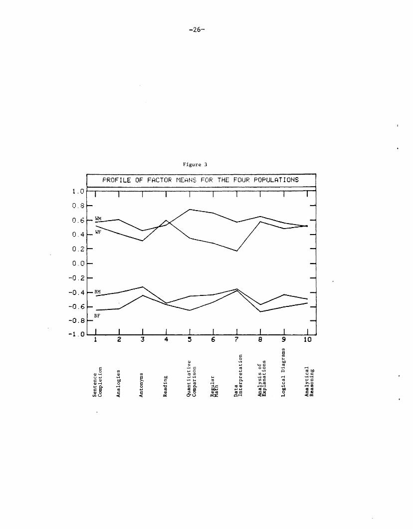
Factor Means

It is customary in item-group interaction studies to define items

that are exceptionally hard for one or more subpopulations as biased

in some sense. These items are then inspected to identify

possible causes for their acting differently for a particular

population. Since information on covariances between items is not

taken into consideration in establishing evidence for whether or not

the items are measuring the same things in the same scale units,

the finding of differentially difficult items may or may not indicate

bias, If it can be established through the analysis of the covariance

structures that items,or logical subsets of items,appear to be measuring

the same things in the same scale units, then the finding of differential

difficulty more likely implies differential achievement rather than bias.

If one starts out with the assumption that the item types describe

different possible ways for processing verbal, mathematical, and analytical

information, and if the data are consistent with an invariant factor

structure across populations, thec,in general,the interpretation of

differences in factor means as differential levels of achievement would

appear to be reasonable.

With this in mind, Figure 3 presents profiles of factor means

by population for the 10 item types. The factor scores are scaled

in terms of standard deviation units with a grand mean of zero.

Inspection of Figure 3 indicates that there are group main effect differences,

as well as some evidence for interaction between group and item-.

type difficulty. It would appear that White females do somewhat less

well in all the quantitative sections while Black females do comparatively

-26-

Figure 3

0.0

-0.2

-0.4

-0.6

-0.8

-1.0

. . PROFILE OF FACTOR NEAt~5 FW? THE FOUR POPULQTIONS

. ,

I I I I I I 1 I I I'

C -

-

- - .

BF -

6 I I I I I 1 I I I , 1 2 3 4 S 6 7 8 9 10

-27-

less well on quantitative comparisons. It appears that both Black

males and females have slightly greater difficulty with the

analysis of explanations item type than with the remaining two

analytical item types. It should be noted that the interactions

are quite small compared to the overall main effect differences.

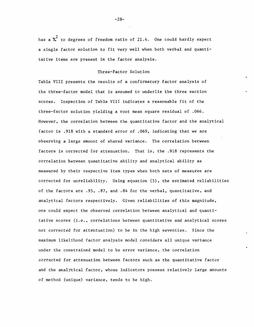
Higher-Order Factor Analysis

Since the preceeding confirmatory tests suggested an invariant

factor structure across populations, the resulting MLH estimate of

the population invariant variance-covariance matrix was used in

fitting the following higher-order factors. A single factor

solution was run to provide base line indices of "goodness of Fit"

to compare with the subsequent more theoretically appropriate models.

The single factor solution shown below:

SINGLE FACTOR SOLUTION

Sentence Completion .922 Analogies .904 Antonyms .821 Reading .810 Quantitative Comparison .706 Regular Math .653 Data Interpretation .576 Analysis of Explanations ,770 Logical Diagrams .640 Analytical Reasoning .726

Root mean square residual = .114

-28-

has a ?L2 to degrees of freedom ratio of 21.4. One could hardly expect

a single factor solution to fit very well when both verbal and quanti-

tative items are present in the factor analysis.

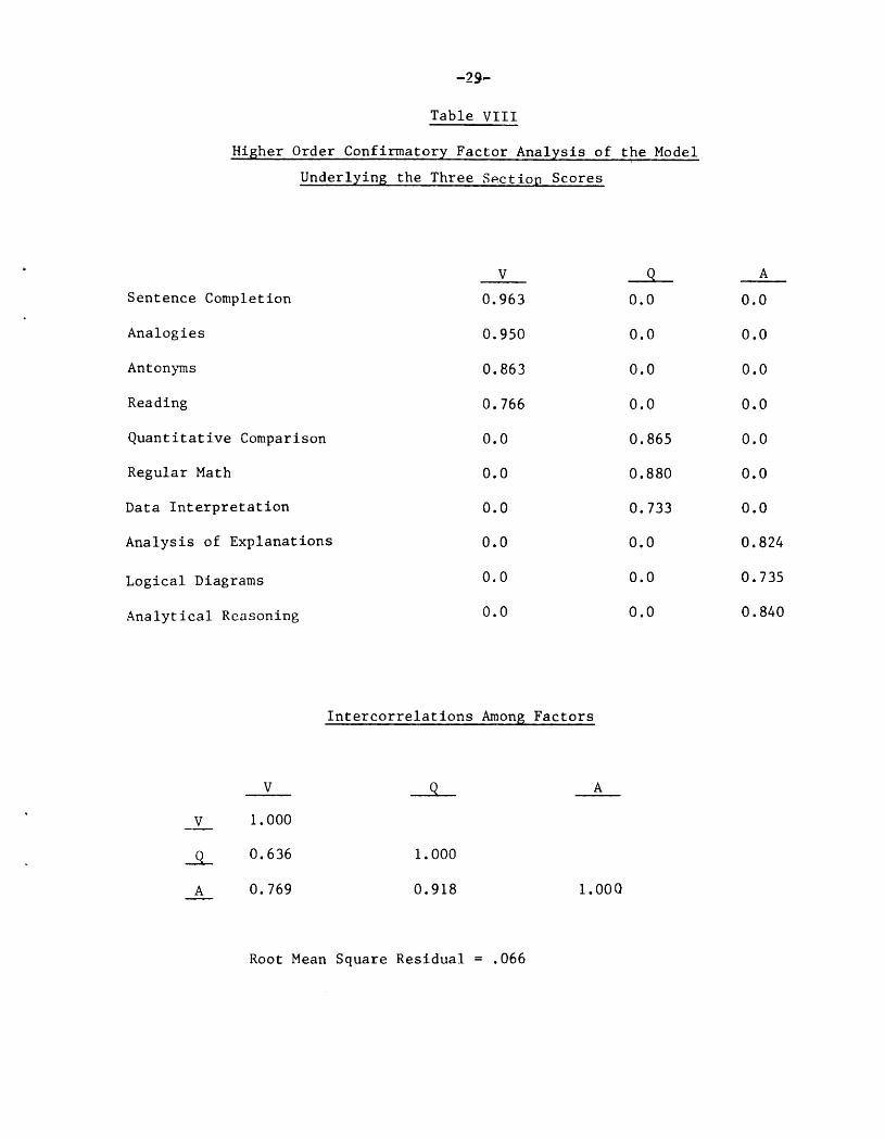
Three-Factor Solution

Table VIII presents the results of a confirmatory factor analysis of

the three-factor model that is assumed to underlie the three section

scores. Inspection of Table VIII indicates a reasonable fit of the

three-factor solution yielding a root mean square residual of .066.

However, the correlation between the quantitative factor and the analytical

factor is .918 with a standard error of .069, indicating that we are

observing a large amount of shared variance. The correlation between

factors is corrected for attenuation, That is, the .918 represents the

correlation between quantitative ability and analytical ability as

measured by their respective item types when both sets of measures are

corrected for unreliability. Using equation (5), the estimated reliabilities

of the factors are .95, .87, and .84 for the verbal, quantitative, and

analytical factors respectively. Given reliabilities of this magnitude,

one could expect the observed correlation between analytical and quanti-

tative scores (i.e., correlations between quantitative and analytical scores

not corrected for attentuation) to be in the high seventies. Since the

maximum likelihood factor analysis model considers all unique variance

under the constrained model to be error variance, the correlation

corrected for attenuation between factors such as the quantitative factor

and the analytical factor, whose indicators possess relatively large amounts

of method (unique) variance, tends to be high.

-29-

Table VIII

Higher Order Confirmatory Factor Analysis of the Model

Underlying the Three Sectiop Scores

Sentence Completion

Analogies

Antonyms

Reading

Quantitative Comparison

Regular Math

Data Interpretation

Analysis of Explanations

Logical Diagrams

Analytical Reasoning

V

0.963

0.950

0.863

0.766

0.0

0.0

0.0

0.0

0.0

0.0

V

V 1.000

Q 0.636

A 0.769

Intercorrelations Among Factors

Q A

1.000

0.918 l.OOQ

Q

0.0

0.0

0.0

0.0

0.865

0.880

0.733

0.0 0.824

0.0

0.0 0.840

A

0.0

0.0

0.0

0.0

0.0

0.0

0.0

0.735

Root Mean Square Residual = ,066

-3o-

Conversely,internal consistency estimates of reliability (espe-

cially split-halves methods) consider shared variance due to the same

method being present in both halves (e.g., split halves of the same item

type) as true variance. These lower bound estimates of reliability

could just as appropriately be referred to as indices of the construct

validity of the weighted composites defining each factor. When congeneric

(i.e., different methods of measuring the same construct) rather than

parallel measures are constrained to define factors, the difference

between reliability and construct validity becomes a "grey" area if not

a meaningless differentiation. We will, however, continue to refer to II

such indices as reliability to be consistent with Joreskog's (1971)

original factorial-based definition of reliability. The important

point here is that when a factor model is constrained to isolate method

variance as error variance,the correlation between factors is likely to

be quite high. The fact that it is so high in this case is not

surprising since one measure of the quantitative factor (data

interpretation) and one measure of the analytical factor (logical

diagrams) have relatively large unique components of method variance.

-31-

Given the considerations above, the correlation between the verbal

and quantitative factors is comparatively low. This particular pattern

of between-factor correlations might be due in part to the selected

population we are dealing with here. That is, if one used the unselected

GRE population (i.e., not just social science majors), one might observe

a somewhat lower correlation between the quantitative and analytical factors

and, conversely, a higher correlation between verbal and quantitative.

Although this three-factor model fits reasonably well, there was a

pattern of residuals associated with the reading comprehension items that

could not be considered zero. That is, after controlling for the verbal

component in reading comprehension (as defined by the first factor), there

remained correlation S (as indicated in the mat rix of residuals

reading a nd measures 0 f bo th quantitat ive abil ity and analytic ability.

between

These correlated residuals run from a low of .lO with regular mathematics to

a high of .20 with analysis of explanations. The X2 to degree of freedom

ratio here was slightly over 8.

In an effort to yield a better "fit", (i.e., reduce residual cor-

relations between reading, mathematical, and analytical items as well

as further investigate the relationship between reading and the other

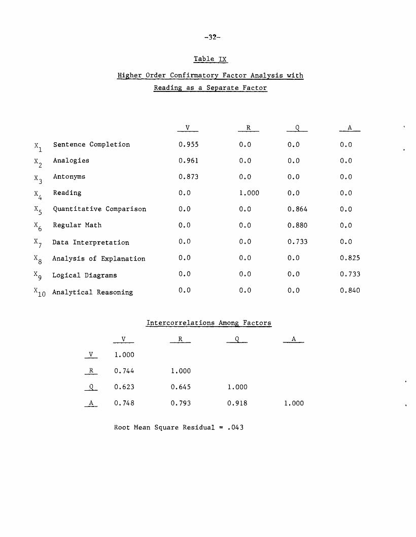
factors), a four-factor confirmatory model was hypothesized, with reading

being a separate factor.

Table IX presents the four-factor solution, which indeed does reduce

the root mean square residuals from -066 to .043 and, not surprisingly,

reduces all the reading related residuals to essentially zero. The X2

to degrees of freedom ratio is approximately 7.

-32-

x1 x2

x3

x4

x5

'6

x7

'8

Table Uz

Higher Order Confirmatory Factor Analysis with

Reading as a Separate Factor

Sentence Completion

Analogies

Antonyms

Reading

Quantitative Comparison

Regular Math

Data Interpretation

Analysis of Explanation

x9 Logical Diagrams

xlQ Analytical Reasoning

v

V 1.000

R 0.744

-Q- 0.623

A 0.748

V

0.955

0.961

0.873

0.0

0.0

0.0

0.0

0.0

R

0.0

0.0

0.0

1.000

0.0

0.0

0.0

0.0

0.0 0.0

0.0 0.0

Intercorrelations Among Factors

R Q

1.000

0.645 1.000

0.793 0.918

Q

0.0

0.0

0.0

0.0

0.864

0.880

0.733

0.0

0.0

0.0

A

1.000

A

0.0

0.0

0.0

0.0

0.0

0.0

0.0

0.825

0.733

0.840

Root Mean Square Residual = ,043

-33-

Inspection of intercorrelations among the factors in Table IX indicates that

reading has a higher relationship with the analytical factor than

it does with the verbal factor. It could well be that the analytical factor

is itself a complex construct sharing variance with reading comprehension

(certainly understan,Jing the directions for analysis of explanations requires

a heavy reading load) and the abstract reasoning present in some mathematical

items such as the quantitative comparison items.

Although the above four-factor solution provides information on the

relationship between the analytical factor and the other factorial com-

ponents of the GRE Aptitude Test, it does not provide much information on

the relationship of the separate analytical item types and the other traditional

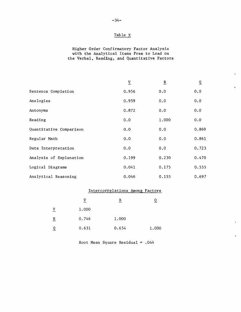
factors. Table X presents a three-factor confirmatory solution where, as before,

the first factor was defined by the three verbal indicators, a second factor was

defined by the reading items,and the third factor was the quantitative factor

defined by the three quantitative item types. The three analytical item types

were left free to load according to the maximum likelihood criterion of best fit.

Inspection of Table X indicates that much of the shared common variance among

the three analytical item types is also common to the quantitative item types.

This;of course, is conststant with the finding of the high unattenuated corre-

lation between the quantitative factor and the analytical factor from the four-

factor solution.

The analysis of explanations item type appears to be somewhat more

factorially complex than either logical diagrams or analytical reasoning. That

is, it has small loadings on both the verbal and reading factors as well as a

substantial loading on the quantitative factor. Analytical reasoning and

logical diagrams have essentially zero loadings on the verbal factor, small

-34-

Table x

Higher Order Confirmatory Factor Analysis with the Analytical Items Free to Load on

the Verbal, Reading, and Quantitative Factors

Sentence Completion

Analogies

Antonyms

Reading

Quantitative Comparison

Regular Math

Data Interpretation

Analysis of Explanation

Logical Diagrams

Analytical Reasoning

V R - -

0.956 0.0

0.959 0.0

0.872 0.0

0.0 1.000

0.0 0.0

0.0 0.0

0.0 0.0

0.199 0.230

0.041 0.175

0.046 0.155

V -

Intercorrelations Among Factors

V R - - 4

1.000

R 0.746 1.000 -

4 0.631 0.654 1.000

9

0.0

0.0

0.0

0.0

0.869

0.861

0.723

0.470

0.555

0.697

Root Mean Square Residual = .044

-35-

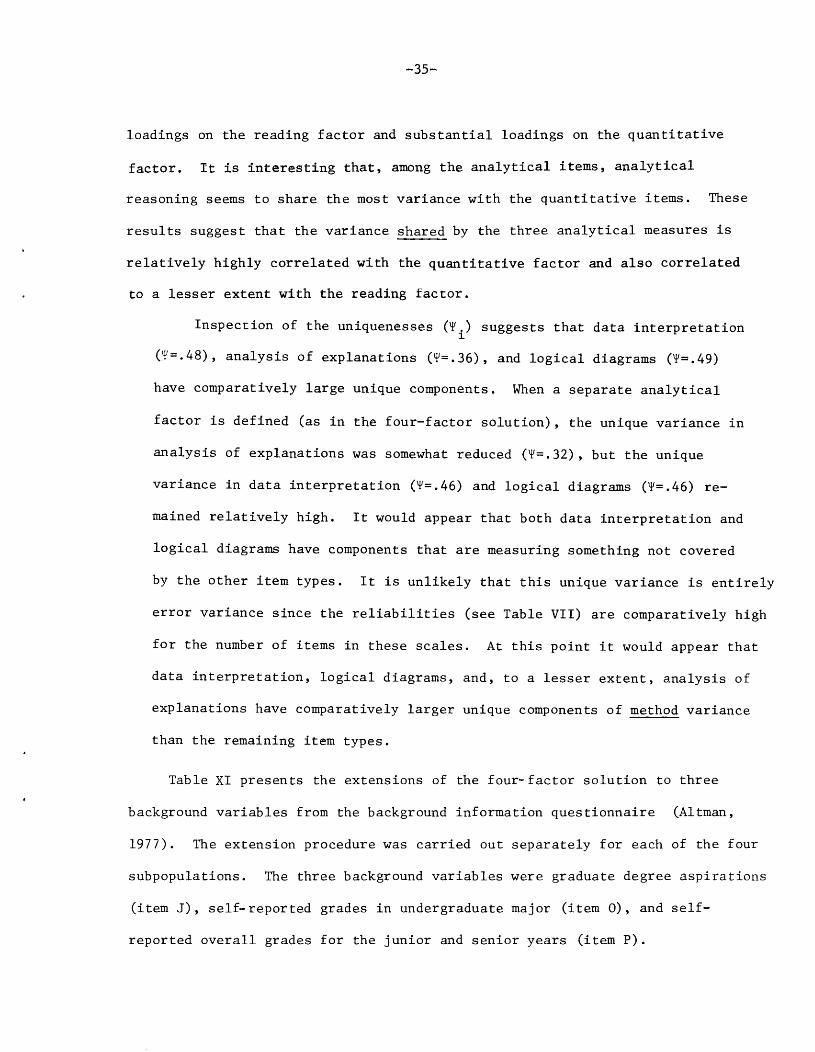
loadings on the reading factor and substantial loadings on the quantitative

factor. It is interesting that, among the analytical items, analytical

reasoning seems to share the most variance with the quantitative items. These

results suggest that the variance shared by the three analytical measures is

relatively highly correlated with the quantitative factor and also correlated

to a lesser extent with the reading factor.

Inspection of the uniquenesses (Yi) suggests that data interpretation

(Y=.48), analysis of explanations (Y=.36), and logical diagrams (Y=.49)

have comparatively large unique components, When a separate analytical

factor is defined (as in the four-factor solution), the unique variance in

analysis of explanations was somewhat reduced (Y=.32), but the unique

variance in data interpretation (Y=.46) and logical diagrams (Y=.46) re-

mained relatively high. It would appear that both data interpretation and

logical diagrams have components that are measuring something not covered

by the other item types. It is unlikely that this unique variance is entirely

error variance since the reliabilities (see Table VII) are comparatively high

for the number of items in these scales. At this point it would appear that

data interpretation, logical diagrams, and, to a lesser extent, analysis of

explanations have comparatively larger unique components of method variance

than the remaining item types.

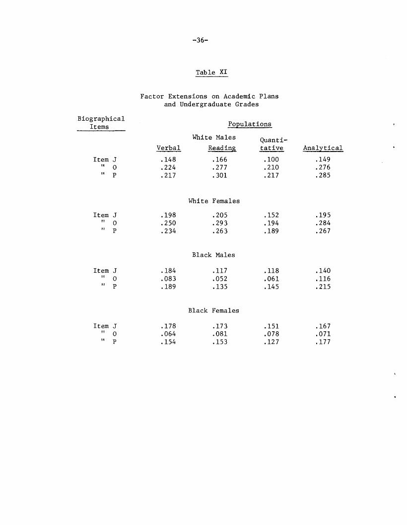
Table XI presents the extensions of the four-factor solution to three

background variables from the background information questionnaire (Altman,

1977). The extension procedure was carried out separately for each of the four

subpopulations. The three background variables were graduate degree aspirations

(item J), self-reported grades in undergraduate major (item 0), and self-

reported overall grades for the junior and senior years (item P).

-360

Table XI

Biographical Items

Factor Extensions on Academic Plans and Undergraduate Grades

Verbal

Item J .148 " 0 .224 " P .217

Item J .198 " 0 .250 " P .234

Item J .184 " 0 .083 " P .189

Item J .178 .173 .151 .167 " 0 .064 .081 .078 .071 " P .154 .153 .127 .177

Populations

White Males Quanti- Reading tative

.166 .lOO

.277 .210

.301 .217

Analytical

.149

.276

.285

White Females

.205

.293

.263

Black Males

.152 .195

.194 .284

.189 ,267

.117 .118

.052

.135

Black Females

.061

.145

.140

.116

.215

-37-

The question here is whether the same patterns of relationship

hold between the extension variables and the four factors within all

subpopulations. Inspection of Table XI indicates that, with one interesting

exception, the pattern of correlations is consistent across populations.

The exception is that the four factors have a proportionately lower

relationship with grades in undergraduate major than with overall junior

and senior grades for the two Black sex groups. It is possible that,

although this analysis has been restricted to social science majors, some

variation still may remain between subpopulations in the major fields being

emphasized. If this is true, then overall junior and senior grades may be

more comparable across populations.

There is a slight tendency for females to show a higher relationship

between their factor scores and their long-term academic aspirations (Item J).

This may reflect in part a greater propensity of males to pursue a particular

career for reasons other than that they seem to have the tested abilities.

In general, the pattern of correlations between the demographics and

verbal, quantitative, and analytical ability scores are similar but lower than

those found by Miller and Wild (1979) for social science majors.

It is somewhat encouraging to note that, while the analytical factor

showed a high unattenuated correlation with the quantitative factor, it showed

a higher "validity" with overall junior and senior grades for all subpopula-

tions than did the quantitative factor. In fact, the analytical factor

showed a higher relationship with past academic performance (grades in

junior and senior year) than did any of the other factors with the exception

of reading.

The results of the extension are consistent with the previous internal

analysis, in that the pattern of the extension coefficients is relatively

-38~

invariant across populations (with the one noted exception). The fact that

the analytical factor shows a slightly higher "validity" than other factors,

except for reading, with past academic performance is not surprising since

the shared variance in the analytical factor is relatively complex, being

related to both the quantitative and reading skill factors. Complex constructs

(such as the analytical factor), as opposed to single-factor measures, are

likely to have higher relationships with complex criteria.

The results of this study are for the most part consistent with the

results of the Swinton and Powers (1980) factor analytic study of the restructured

GRE Aptitude Test. Using exploratory factor analytic procedures, Swinton

and Powers defined the following oblique factors: (1) reading comprehension,

(2) vocabulary, (3) quantitative ability, and (4) analytical reasoning.

Similar to the results of the present study, the analytical factor was found

to be highly correlated with the reading and quantitative factors. Although

the absolute magnitude of the correlations was lower than that found in the

present confirmatory study, this discrepancy can be partially explained by

differences in methodological approaches. Swinton and Powers found that the

analysis of explanations item type was internally complex while our confirma-

tory procedures also suggested that, among the analytical item types, it was

the most complex. The finding by both studies of a separate reading factor

relatively highly correlated with the analytical factor (and, to a lesser

extent, with the other factors) yielded independent evidence of the primacy

of the reading construct in all test items. Swinton and Powers found that

past academic achievement was positively related to all GRE Aptitude Test

factors, as did this study.

-39-

With respect to logical diagrams, Swinton and Powers found them

to be factorially complex, although apparently less so than analysis

of explanations. This study also found them to be somewhat complex

(and less so than analysis of explanations) but to also have a relatively

large component of unique (possibly method) variance.

Comparison of ethnic and sex differences from the two studies showed

similar results. Although not specifically shown, Swinton and Powers

state that the ranks of the ethnic groups remain relatively stable across

their factors. Similar results are suggested from the factor scores of

this study. The Blacks' relative position on the factors is fairly stable,

with a minor drop on the quantitative and analysis of explanations items.

Sex group factor score means lead to similar conclusions for both studies,

with the exception that, in this study, White female means do not exceed White

male means except for reading comprehension. These slight differences in

findings are possibly due to the confounding of sex and ethnic differences

with fields of study.

In summary, the two studies arrive at reasonably similar conclusions

using quite dissimilar methodologies and samples. The Swinton and Powers

study examined the factorial structure of the GRE Aptitude Test within a

single heterogeneous population. They then investigated a number of re-

lationships between external biographical information and the obtained factor

structure within that population. The present study investigated the

possibility of an invariant GRE factor structure across sex and ethnic

groups, controlling for major field of study. After developing a relatively

invariant factor structure, a limited number of external biographical

-4o-

variables were then related to the factor structure within each population.

The results of the confirmatory study developed additional evidence for

the presence and complexity of the factors identified in the Swinton and

Powers study and further demonstrated the invariance of selected psycho-

metric characteristics of the factors across ethnic and sex groups.

Summary and Conclusions

The primary purpose of this study was to: (1) evaluate the invariance of

the internal structure construct validity and thus the interpretation of

GRE Aptitude Test scores across four populations, and (2) develop and

apply a systematic procedure for investigating the possibility of test

bias from a construct validity frame of reference. The notion of invariant

construct validity was defined as (1) similar patterns of loadings across

populations, (2) equal units of measurement across populations, and (3)

equal test score precision as defined by the standard error of measurement.

Although other forms of bias might exist that would not be identified

by these procedures, if any one of the above criteria differs across

populations, then one has to consider seriously the possibility of psychometric

bias, as defined in this paper. The advantage of investigating psychometric

bias at the item type level (even though the total score may not be biased)

is that this may provide an "early warning" with respect to any future plans

to increase the number of items of any particular type. A secondary purpose

of this study was to evaluate the factor structure of the three sections (verbal,

quantitative and analytical) from which section scores are derived. Assuming

-41-

that the invariant construct validity model based on item types is tenable,

a hypothesized three factor "macro" model based on the three sections

could be carried out on the population invariant variance-covariance matrix.

It should be noted that the term "psychometric bias" as defined

here does not require external criteria information for the analysis. The

internal procedure used here is suggested as only a first step in a broader

process of an integrated validation procedure that should include not only

internal checks on the population invariance of the underlying constructs but

also checks on the population invariance of their relationships with external

criteria. Although this is only a first step, it is a necessary step since any

interpretation of relationships with external criteria becomes academic unless

one can first show that the tests measure what they purport to measure with

similar meaning and accuracy for all populations of interest.

The four subpopulations were 1,122 White males, 1,471 White females,

284 Black males, and 626 Black 'females.

The analysis indicated that a factor structure defined by the 10

item types showed relatively invariant psychometric characteristics across

the four subpopulations. That is, the item-type factors appear to be

measuring the same things in the same units with the same precision. There

does not appear to be any significant evidence of psychometric bias in the

test.

Confirmatory analysis of a higher-order factor model defined by an

a griori model based on three- and four-factor solutions was attempted to

investigate the factorial contributions of the analytical item types.

-42-

Results of this analysis indicated that the three analytical item types

appear to be varying functions of reading comprehension and quantitative

ability. The analysis of explanations item type was the more complex

factorially and included a vocabulary component as well as reading and

quantitative components. Of the remaining two analytic item types,

logical diagrams had the comparatively larger unique variance component.

Analytical reasoning appear to share most of its variance with the reading

comprehension and quantitative factors.

It would seem that of the analytical item types, logical diagrams

has the greatest possibility of adding unique yet reliable variance to

the GRE Aptitude Test while analytical reasoning items appear to add the

least amount of new information. Analysis of explanations is the most

factorially complex but its multidimensionality is to a great extent

described by the already present verbal, reading comprehension, and quanti-

tative factors. For other views see Darlington (1971) and Schmidt and

Hunter (1976).

-43-

References

Altman, R. A. A summary of data collected from Graduate Records Examination

test-takers during 1976-1977. Data Summary Report #2, Princeton, N.J.:

Educational Testing Service, 1977.

Campbell, D., & Fiske, D. Convergent and discriminant validation by the

multitrait-multimethod matrix. Psychological Bulletin, 1959, 56,

81-105.

Cleary, A. Test Bias: Prediction of grades of Negro and White students

in integrated colleges. Journal of Educational Measurement, 1968,

5, 113-124.

Cronbach, L. J. Test validation. In R. Thorndike (Ed.), Educational

Measurement. Washington, D.C.: American Council on Education, 1971.

Darlington, R. B. Another look at "Cultural Fairness." Journal of Educational

Measurement. 1971, &, 71-82.

Jb'reskog, K. G. Statistical analysis of sets of congeneric tests. Psychometrika,

1971, 36, 109-133.

Miller, R., & Wild, C. I,. (Eds.) Restructuring the Graduate Record Examin-

ations Aptitude Test. GRE Board Technical Report. Princeton, N.J.:

Educational Testing Service, 1979.

Rock, D. A., & Werts, C. E. Construct validity of the SAT across populations--

An empirical confirmatory study. Research Report RR-79-2. Princeton,

N.J.: Educational Testing Service, 1979.

Schmidt, F. L., & Hunter, J. E. Critical analysis of the statistical and ethical

implications of various definitions of test bias. Psychological Bulletin,

1976, 83(6), 1053-1071.

-44-

Sb'rbom, D. A general method for studying differences in factor means and

factor structure between groups. British Journal of Mathematical and

Statistical Psychology, 1974, 27, 229-239.

S&born, D., 6 Jsreskog, K. G. COFAMM: Confirmatory factor analysis with

model identification. User's guide. Chicago, Illinois: National

Educational Resources, Inc. 1976.

Swinton, S. S., 6 Powers, D. E. A factor analytic study of the restructured

GRE Aptitude Test. GRE Board Professional Report No. 77-6P, Princeton,

N.J.: Educational Testing Service, 1980.

Wiley, D. E. The identification problem for structural equation models

with unmeasured variables. In A. S. Goldberger & 0. D. Duncan (Eds.),

Structured equation models in the social sciences. New York: Seminar

Press, 1973.

bpendix A

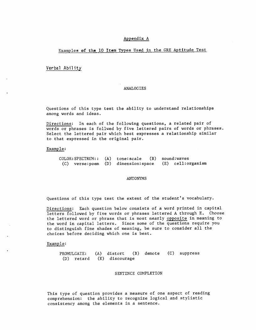
Examples of the 10 Item Types Used in the GRE Aptitude Test

Verbal Ability

ANALOGIES

Questions of this type test the ability to understand relationships among words and ideas.

Directions: In each of the following questions, a related pair of words or phrases is follwed by five lettered pairs of words or phrases. Select the lettered pair which best expresses a relationship similar to that expressed in the original pair.

Example:

COLOR:SPECTRUM:: (A) tone:scale (B) sound:waves

(C) verse:poem (D) dimension:space (E) cell:organism

ANTONYMS

Questions of this type test the extent of the student's vocabulary.

Directions: Each question below consists of a word printed in capital letters followed by five words or phrases lettered A through E. Choose the lettered word or phrase that is most nearly opposite in meaning to the word in capital letters. Since some of the questions require you to distinguish fine shades of meaning, be sure to consider all the choices before deciding which one is best.

Examnle:

PROMULGATE: (A) distort (B) demote (C) suppress

(D) retard (E) discourage

SENTENCE COMPLETION

This type of question provides a measure of one aspect of reading comprehension: the ability to recognize logical and stylistic consistency among the elements in a sentence.

-2-

Directions: Each of the sentences below has one or more blank spaces, each blank indicating that a word has been omitted. Beneath the sentence are five lettered words or sets of words. You are to choose the one word or set of words which, when inserted in the sentence, best fits in with the meaning of the sentence as a whole.

Example:

Early ------- of hearing loss is ------- by the fact that the other senses are able to compensate for moderate amounts of loss, so that people frequently do not know that their hearing is imperfect.

(A) discovery..indicated (B) development..prevented (C) detection..complicated (D) treatment..facilitated

(E) incidence..corrected

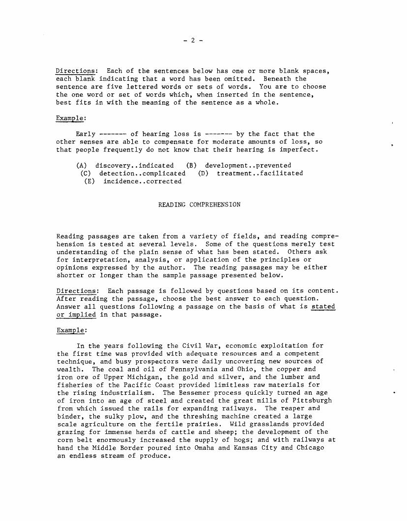
READING COMPREHENSION

Reading passages are taken from a variety of fields, and reading compre- hension is tested at several levels. Some of the questions merely test understanding of the plain sense of what has been stated. Others ask for interpretation, analysis, or application of the principles or opinions expressed by the author. The reading passages may be either shorter or longer than the sample passage presented below.

Directions: Each passage is followed by questions based on its content. After reading the passage, choose the best answer to each question. Answer all questions following a passage on the basis of what is stated or implied in that passage.

Example:

In the years following the Civil War, economic exploitation for the first time was provided with adequate resources and a competent technique, and busy prospectors were daily uncovering new sources of wealth. The coal and oil of Pennsylvania and Ohio, the copper and iron ore of Upper Michigan, the gold and silver, and the lumber and fisheries of the Pacific Coast provided limitless raw materials for the rising industrialism. The Bessemer process quickly turned an age of iron into an age of steel and created the great mills of Pittsburgh from which issued the rails for expanding railways. The reaper and binder, the sulky plow, and the threshing machine created a large scale agriculture on the fertile prairies. Wild grasslands provided grazing for immense herds of cattle and sheep; the development of the corn belt enormously increased the supply of hogs; and with railways at hand the Middle Border poured into Omaha and Kansas City and Chicago an endless stream of produce.

-3-

As the line of the frontier pushed westward, new towns were built, thousands of claims to homesteads were filed, and speculator and pro- moter hovered over the prairies like buzzards seeking their carrion. With rising land values money was to be made out of unearned increment, and the creation of booms was a profitable industry. The times were stirring, and it was a shiftless fellow Rho did not make his pile. If he had been too late to file on desirable acres, he had only to find a careless homesteader who had failed in some legal technicality and "jump his claim." Good bottom land could be had even by late-comers if they were sharp at the game.

The bustling America of 1870 accounted itself a democratic world. A free people had put away all aristocratic privileges and, conscious of power, had gone forth to possess the last frontier. But America's essential social philosophy, which it found adequate to its needs, was summed up in three words -- preemption, exploitation, progress. Its immediate and pressing business was to dispossess the government of its rich holdings. Lands in the possession of the government were so much idle waste, untaxed and profitless; in private hands they would be developed. They would provide work, pay taxes, support schools, enrich the community. Preemption meant exploitation and exploitation meant progress.

It was a simple philosophy and it suited the simple individualism of the times. The Gilded Age knew nothing of enlightenment; it recog- nized only the acquisitive instinct. That much at least the frontier had taught the great American democracy; and in applying to the resources of a continent the lesson it had been so well taught, the Gilded Age wrote a profoundly characteristic chapter of American history.

According to the passage, increased corn production was mainly responsible for an increase in the

(A) number of sheep (B) output of farm implements (0 supply of hogs (D) amount of pasture land

(ES number of cattle

Quantitative Ability

REGULAR MATH AND GRAPHS

Directions: Solve each of the following problems, using any available space on the page for scratch work. Then indicate the best answer in the appropriate space on the answer sheet.

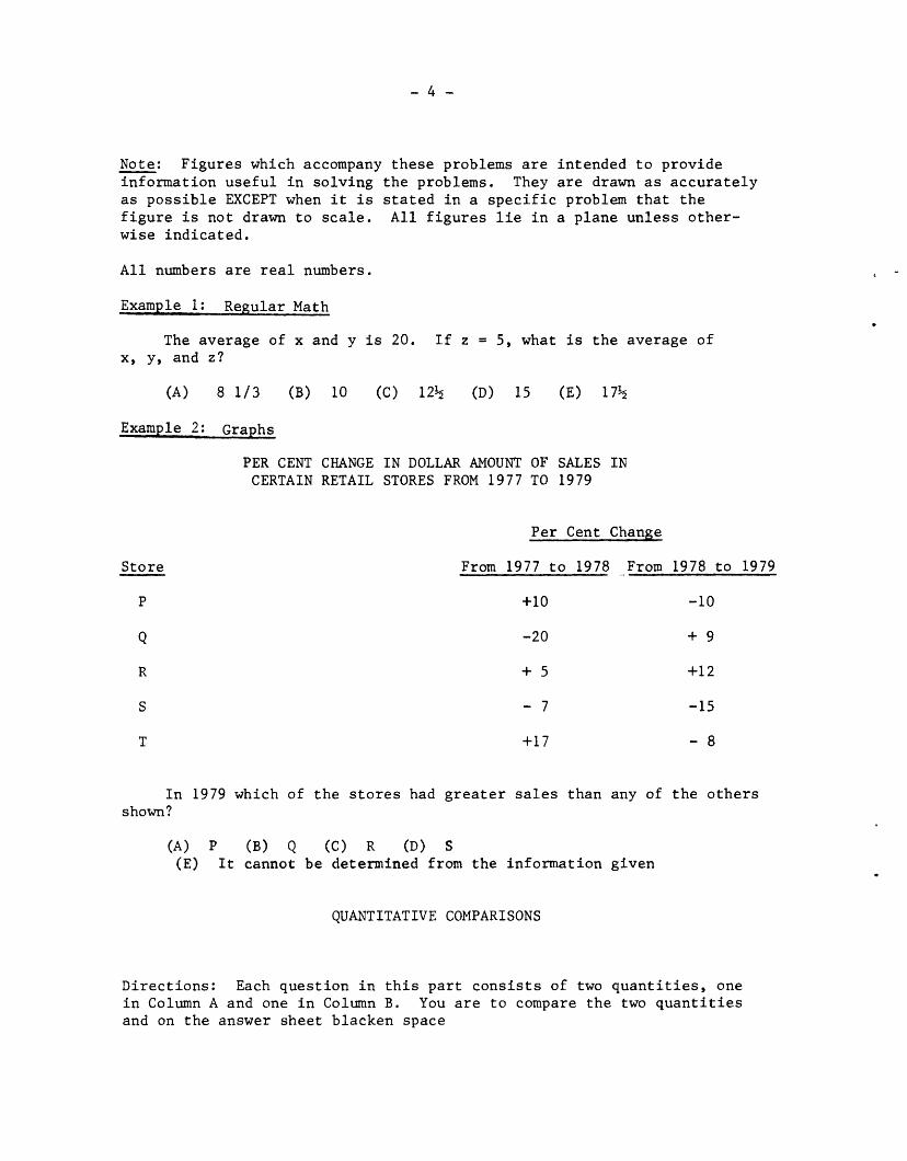
-4-

Note: Figures which accompany these problems are intended to provide information useful in solving the problems. They are drawn as accurately as possible EXCEPT when it is stated in a specific problem that the figure is not drawn to scale. All figures lie in a plane unless other- wise indicated.

All numbers are real numbers.

Example 1: Regular Math

The average of x and y is 20. If z = 5, what is the average of x, y, and z?

(A) 8 l/3 (B)

Example 2: Graphs

PER CENT CERTAIN

Store

10 (c) 12% (D) 15 (E) 17%

CHANGE IN DOLLAR AMOUNT OF SALES IN RETAIL STORES FROM 1977 TO 1979

Per Cent Change

From 1977 to 1978 .-From 1978 to 1979

+10 -10

-20 +9

+5 +12

-7 -15

+17 -8

In 1979 which of the stores had greater sales than any of the others shown?

(A) P (B) Q CC) R (D) S (E) It cannot be determined from the information given

QUANTITATIVE COMPARISONS

.

Directions: Each question in this part consists of two quantities, one in Column A and one in Column B. You are to compare the two quantities and on the answer sheet blacken space

-5-

A if the quantity in Column A is the greater;

B if the quantity in Column B is the greater;

C if the two quantities are equal;

D if the relationship cannot be determined from the information given.

Common Information: In a question, information concerning one or both of the quantities to be compared is centered above the two columns. A symbol that appears in both columns represents the same thing in Column A as it does in Column B.

Numbers: All numbers used are real numbers; all square roots are positive numbers.

Figures: Position of points, angles, regions, etc. can be assumed to be in the order shown.

Lines shown as straight can be assumed to be straight.

Figures are assumed to lie in the plane unless otherwise indicated.

Figures which accompany questions are intended to provide information useful in answering the questions. However, a figure is drawn to scale, you should solve estimating sizes by sight or by measurement, of mathematics.

unless a note states that these problems NOT by but by using your knowledge

Example:

Column A Column B

2x6 2+6

Analytical Ability

ANALYSIS OF EXPLANATIONS

Directions: For each set of questions, a fact situation and a result are presented. Several numbered statements follow the result. Each statement is to be evaluated in relation to the fact situation and result.

-6-

Consider each statement separately from the other statements. For each one, examine the following sequence of decisions, in the order A,B,C,D,E. Each decision results in selecting or eliminating a choice. The first choice that cannot be eliminated is the correct answer.

A Is the statement inconsistent with, or contradictory to, something in the fact situation, the result, or both together? If so, choose A.

If not,

B Does the statement present a possible adequate explanation of the result? If so, choose B.

If not,

C Does the statement have to be true if the fact situation and result are as stated? If so, the statement is deducible from something in the fact situation, the result, or both together; choose C.

If not,

D Does the statement either support or weaken a possible explanation of the result? If so, the statement is relevant to an explanation: choose D.

E If not, the statement is irrelevant to an explanation of the result; choose E.

Use common sense to decide whether explanations are adequate and whether statements are inconsistent or deducible. No formal system of logic is presupposed. Do not consider extremely unlikely or remote possibilities.

Example:

Situation. In an attempt to end the theft of books from Parkman University Library, Elnora Johnson, the chief librarian, initiated a stringent inspection program at the beginning of the fall term. At the library entrance, Johnson posted inspectors to check that each library book leaving the building had a checkout slip bearing the call number of the book, its due date, and the borrower's identification number. The library retained a carbon copy of this slip as its only record that the book had been checked out. Ju-nnsonordered the inspec- tors to search for concealed library books in attachk cases, bookbags, and all other containers large enough to hold a book. Since no new personnel could be hired, all library personnel took turns serving as inspectors, though many complained of their embarrassment in conducting the searches.

Result. During that term Margaret Zimmer stole twenty-five library books.

Statement. Zimmer stole the books before the inspection began.

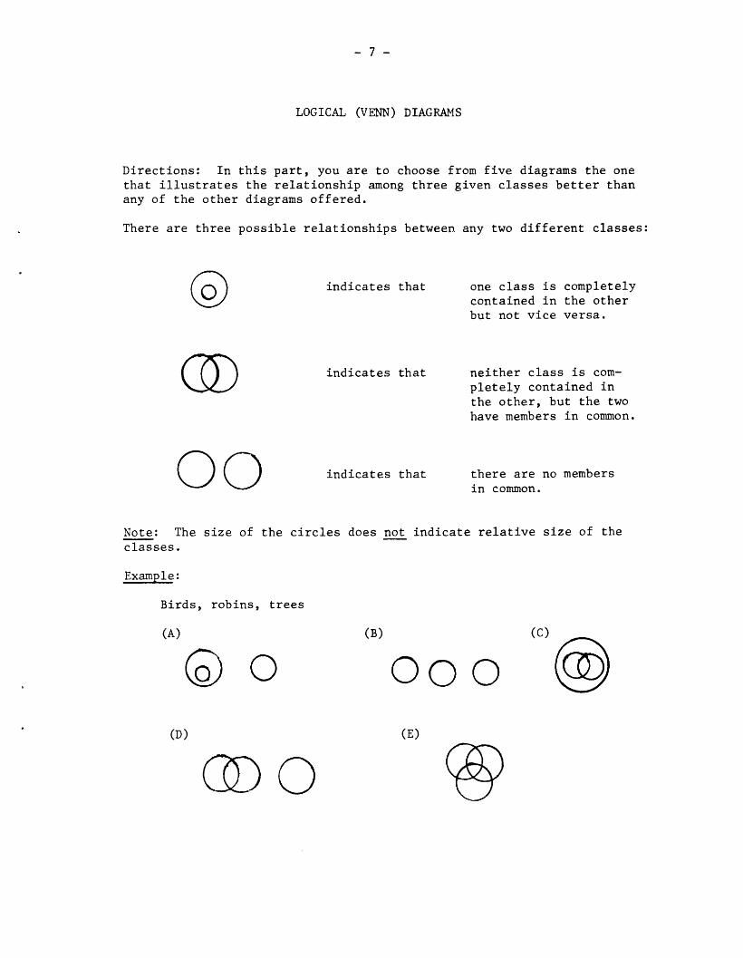
-7-

LOGICAL (UN-N) DIAGRAMS

Directions: In this part, you are to choose from five diagrams the one that illustrates the relationship among three given classes better than any of the other diagrams offered.

There are three possible relationships between any two different classes:

0 0 indicates that one class is completely contained in the other but not vice versa.

indicates that neither class is com- pletely contained in the other, but the two have members in common.

00 indicates that there are no members in common.

Note: The size of the circles does not indicate relative size of the classes.

Example:

Birds, robins, trees

(A)

CD) (E)

CD0 0

-8-

ANALYTICAL REASONING

Directions: Each question or group of questions is based on a passage or set of statements. In answering some of the questions it may be useful to draw a rough diagram. Choose the best answer for each question and blacken the corresponding space on your answer sheet.

Examnle:

(1) It is assumed that a half tone is the smallest possible interval between notes.

(2) Note T is a half tone higher than note V,

(3) Note V is a whole tone higher than note W.

(4) Note W is a half tone lower than note X.

(5) Note X is a whole tone lower than note T.

(6) Note Y is a whole tone lower than note W.

Which of the following represents the relative order of the notes from lowest to highest?

(A) X Y W V T (B) Y W X V T (C) W V T Y X (D) Y W V T X (E) Y X W V T

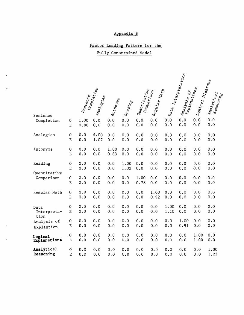
Appendix B

Factor Loading Pattern for the

Fully Constrained Model

Sentence Completion

Analogies

Antonyms

Reading

Quantitative Comparison

Regular Math

Data Interpreta- tion

Analysis of Explantion

Logical Explanations

Analytical Reasoning

0

E

0 E

0 E

0 E

0 E

0 E

0 E

0 E

0 E

0 E

1.00 0.80

0.0 0.0

0.0 0.0

0.0 0.0

0.0 0.0

0.0 0.0

0.0 0.0

0.0 0.0

0.0 0.0

0.0 0.0

_ -2

0.0 0.0

LOO 1.07

0.0 0.0

0.0 0.0

0.0 0.0

0.0 0.0

0.0 0.0

0.0 0.0

0.0 0.0

0.0 0.0

0.0 0.0

1.00 0.83

0.0 0.0

0.0 0.0

0.0 0.0

0.0 0.0

0.0 0.0

0.0 0.0

0.0 0.0

‘rv z 2

0.0 0.0

0.0 0.0

0.0 0.0

1.00 1.02

0.0 0.0

0.0 0.0

0.0 0.0

0.0 0.0

0.0 0.0

0.0 0.0

0.0 0.0

0.0 0.0

0.0 0.0

0.0 0.0

1.00 0.78

0.0 0.0

0.0 0.0

0.0 0.0

0.0 0.0

0.0 0.0

0.0 0.0 0.0 0.0

0.0 0.0 0.0 0.0

0.0 0.0 0.0 0.0

0.0 0.0 0.0 0.0

0.0 0.0 0.0 0.0

1.00 0.0 0.92 0.0

0.0 1.00 0.0 1.10

0.0 0.0 0.0 0.0

0.0 0.0 0.0 0.0

0.0 0.0

G 0.0 0.0

0.0 0.0

0.0 0.0

0.0 0.0

0.0 0.0

0.0 0.0

0.0 0.0

0.0 0.0

1.00 1.00

0.0 0.0 0.0 0.0 0.0 1.22

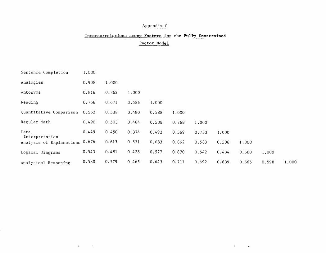
Appendix C

Intercorrelations among Factors for the PulIy Constrained

Factor Model

Sentence Completion 1.000

Analogies 0.908

Antonyms 0.816

Rezding 0.766

Quantitative Comparison 0.552

Regular Nath 0.490

Data 0.449 Interpretation

Analysis of Explanations 0.676

Logical Diagrams 0.543

Analytical Reasoning 0.580

1.000

0.862

0.671

0.538

0.503

0.450

0.613

0.481

0.579

1.000

0.586 1.000

0.480 0.588 1.000

0.464 0.538 0.768 1.000

0.374 0.493 0.569 0.733 1.000

0.531 0.683 0.662 0.583 0.506 1.000

0.428 0.577 0.670 0.542 0.434 0.680 1.000

0.465 0.643 0.711 0.692 0.639 0.665 0.598 1.000

GRE BOARD RESEARCH REPORTS OF A TECHNICAL NATURE

Boldt, R. R. Comparison of a Bayesian and a Least Squares Method of Educational Prediction. GREB No. 7O-3P, June 1975.

Campbell, J. T. and Belcher, L. H. Powers, D. E.; Swinton, S.; Thayer, D.; Word Associations of Students at and Yates, A. A Factor Analytic Predominantly White and Predominantly Investigation of Seven Experimental Black Colleges. GREB No. 71-6P, Analytical Item Types. GREB No. December 1975. 77-lP, June 1978.

Campbell, J. T. and Donlon, T. F. Relation- ship of the Figure Location Test to Choice of Graduate Major. GREB No. 75-7P, November 1980.

Carlson, A. B.; Reilly, R. R.; Mahoney, M. H * and Casserly, P. L. The DLielopment and Pilot Testing of Criterion Rating Scales. GREB No. 73-lP, October 1976.

Carlson, A. B.; Evans, F.R.; and Kuykendall, N. M. The Feasibility of Common Criterion Validity Studies of the GRE. GREB No. 71-lP, July 1974.

Donlon, T. F. An Exploratory Study of the Implications of Test Speededness. GREB No. 76-9P, March 1980.

Donlon, T. F.; Reilly, R. R.; and McKee, J. D. Development of a Test of Global vs. Articulated Thinking: The Figure Location Test. GREB No. 74-9P, June 1978.

Echternacht, G. Alternate Methods of Equating GRE Advanced Tests. GRE‘B No. 69-2P, June 1974.

Echternacht, G. A Comparison of Various Item Option Weighting Schemes/A Note on the Variances of Empirically Derived Option Scoring Weights. GREB No. 71-17P, February 1975.

Echternacht, G. A Quick Method for Determining Test Bias. GREB No. 70-8P, July 1974.

Evans, F. R. The GRE-Q Coaching/Instruction Study. GREB No. 71-5aP, September 1977.

Fredericksen, N. and Ward, W. C. Develop- ment of Measures for the Study of Creativity. GREB No. 72-2P, June 1975.

Levine, M. V. and Drasgow, F. Appropriate- ness Measurement with Aptitude Test Data and Esimated Parameters. GREB No. 75-3P, March 1980.

McPeek, M.; Altman, R. A.; Wallmark, M.; and Wingersky, B. C. An Investigation of the Feasibility of Obtaining Additional Subscores on the GRE Advanced Psychology Test. GREB No. 74-4P, April 1976.

Pike, L. Implicit Guessing Strategies of GRE Aptitude Examinees Classified by Ethnic Group and Sex. GREB No. 75-lOP, June 1980.

Powers, D. E.; Swinton, S. S.; and Carlson, A. B. A Factor Analytic Study of the GRE Aptitude Test. GREB No.

75-llP, September 1977.

Reilly, R. R. and Jackson, R. Effects

of Empirical Option Weighting on Reliability and Validity of the GRE. GREB No. 71-9P, July 1974.

Reilly, R: R. Factors in Graduate Student Performance. GREB No. 71-2P, July 1974.

Rock, D. A. The Identification of Population Moderators and Their Effect on the Prediction of Doctorate Attainment. GREB No. 69-hbP, February 1975.

Rock, D. A. The "Test Chooser": A Different Approach to a Prediction Weighting Scheme. GREB No. 70-2P, November 1974.

Sharon, A. T. Test of English as a Foreign Language as a Moderator of Graduate Record Examinations Scores in the Prediction of Foreign Students' Grades in Graduate School. GREB No. 70-lP, June 1974.

Stricker, L. J. A New Index of Differential Subgroup Performance: Application to the GRE Aptitude Test. GREB No. 78-7P, June 1981.

Swinton, S. S. and Powers, D. E. A Factor Analytic Study of the Restructured GRE Aptitude Test. GREB No. 77-6P, February 1980.

Ward, W. C. A Comparison of Free-Response and Multiple-Choice Forms of Verbal Aptitude Tests. GREB No. 79-8P, January 1982.

Ward, W. C.; Frederiksen, N.; and Carlson, S. B. Construct Validity of Free- Response and Machine-Storable Versions of a Test of Scientific Thinking. GKEB No. 74-8P, November 1978.

Ward, W. C. and Frederiksen, N. A Study of the Predictive Validity of the Tests of Scientific Thinking. GREB No. 74-6P, October 1977.