US aggregate demand for clothing and shoes: effects of non-durable expenditures, price and demographic changes

© 2003 Blackwell Publishing Ltd

International Journal of Consumer Studies,

27

, 2, March 2003, pp111–125

111

Blackwell Science, LtdOxford, UKJCSInternational Journal of Consumer Studies0309-3891Blackwell Publishing Ltd, 200327Original Article

US aggregate demand for

clothing and shoes

K. Kim

Correspondence

Kisung Kim, Department of Home Science and Industry, College of Science and Engineering, Sangji University, Woosan-dong, Wonju, Kangwon, South Korea, 220-702. E-mail: [email protected]

US aggregate demand for clothing and shoes: effects of non-durable expenditures, price and demographic changes

Kisung Kim

Department of Home Science and Industry, College of Science and Engineering, Sangji University, Kangwon, South Korea

Abstract

The main objective of this study was to evaluate the effects

of the changes in total non-durables expenditures, prices

and US demographics on demand for different clothing cat-

egories and shoes in a time-series framework. The basis for

the demand model was the almost ideal demand system

model. Demographic variables included in the model were

age distribution of US population (median age and variance)

and proportion of non-white population to the total US

population. The results indicate that total non-durable

expenditures and price variables are significantly related to

consumers’ non-durable budget allocations for clothing cat-

egories and shoes. The results of the study also show that,

among the demographic variables examined in the study, the

median age and non-white population were significant

variables affecting US aggregate non-durable expenditure

allocation on men’s and boy’s clothing and shoes. All the

demand elasticities with respect to total expenditures, own,

cross-price and demographics were also estimated.

Keywords

Clothing

,

shoes

,

expenditure

,

demand

,

elasticity

,

demographic

.

Introduction

The US has had many changes in population structureover the past several decades. The US is ageing in twodominant ways that include the ageing baby-boomergeneration and the increased numbers of elderly people(65 years over). The adult population between 30 and50 years in the US is expanding. The median age of theUS population in 1994 was 34 years, which was 4 yearsolder than the median age in the 1980 Census.

1

The USpopulation has also become more diverse in racial and

ethnic composition. As blacks, American Indians,Asians and Hispanics have increased their proportionsof the total population, the white proportion of thepopulation has declined.

1

By the turn of the century, thewhite proportion of the population is projected to be<82%.

1

Based on the data in the National Income and Prod-uct Accounts of the US (NIPA),

2–4

consumer expendi-ture categories have changed in importance in the USover the past 60 years. For example, the shares of per-sonal consumption expenditures for food, medical care,recreation and housing have changed substantially. Theexpenditure share of clothing and shoes in personal con-sumption expenditures in nominal terms decreasedfrom 12.1% in 1929 to 5.3% in 1994. The share of cloth-ing and shoes in real personal consumption expendi-tures decreased from 7.4% in 1929 to 4.5% in 1970, butthe share has increased since 1970, reaching 5.8% in1994 (Fig. 1). According to the NIPA price indexes forpersonal consumption expenditures by type of product,the price for clothing items and shoes increased faster,at an average annual rate of 1.7%, than the price of allgoods together during the years 1930–70. During 1971–94, the price of all goods rose faster than the price ofclothing and shoes, which rose 5.33% per year on aver-age (Table 1). Combined with the lowered relative priceof clothing and shoes, the increased real expenditureshare of clothing and shoes may indicate that the pur-chased quantity of clothing has increased relative to thatof all goods since the early 1970s.

Despite the remarkable changes in demographiccharacteristics (i.e. age and race/ethnicity) and in expen-diture allocation among consumption goods in the US,information regarding the demand patterns for clothingcategories and shoes is limited. Many cross-sectionalanalyses on US clothing consumption have incorpo-rated demographic variables. The cross-sectional studieshave mainly used a single equation approach by assum-ing that a household’s or consumer’s decisions about

US aggregate demand for clothing and shoes

•

K. Kim

112


27

, 2, March 2003, pp111–125


expenditures on clothing were independent of itsdecisions about expenditure on other commodities.

3

Also, because of data availability, such studies have notusually addressed price effects. Within the time-seriesframework, some studies of clothing consumptionexpenditure have been conducted. Previous time-serieshave focused on the estimation of clothing consumptionas one consumption category.

5–9

Houthakker andTaylor

10

and Blanciforti

et al

.

11

conducted comprehen-sive demand analyses of different categories of con-sumption goods, but these studies lacked the effects ofdemographic variables on clothing categories and shoes.No demand analysis of clothing categories (i.e. women’sand children’s clothing, men’s and boys’ clothing) andshoes has been conducted with a demand system thataccounts for the interdependence of consumer decisionmaking in purchasing goods. The present researchfocuses on analysing those US aggregate demands,incorporating the selected demographic variables in ademand system in a time-series framework.

This study has two main objectives. The first objectiveis to evaluate the effect of the changes in total expendi-tures and prices on US aggregate demands for women’sand children’s clothing, men’s and boys’ clothing andshoes. The second objective is to determine the impactsof the changes in selected demographic variables (i.e.median age, age distribution of US population and ratioof non-white to total US population) on US aggregatedemands for those clothing categories and shoes. Toaddress the objectives of the study, the almost idealdemand system (AIDS) model developed by Deatonand Muellbauer

12

was used.

Previous research

Most cross-sectional studies used age of householdheads or reference persons as an age variable. House-hold expenditure for clothing declines with increasedage of household head

8,13–15

and, in parent–child house-holds, the highest expenditures tend to occur when theparents are in their forties.

16

Multivariate analysis of the1972–73 Consumer Expenditure Survey (CES) data hasshown that expenditures on clothing decline in the laterstages of the family life cycle,

14

which the researchersattributed to the accumulation of clothing inventoriesover the family life cycle and to rising expenditures for

Figure 1

Clothing and shoes expenditures as a share of total personal consumption expenditures, 1929–94. Clothing and shoes expenditure shares were calculated and plotted using the data in statistical tables (Tables 2.6 and 2.7) in The National Income and Product Accounts of the US, 1929–58, 1959–88, 1985–92, 1993–94, US Department of Commerce, Bureau of Economic Analysis, Washington, DC. The shares in 1987 dollars differ from the nominal shares because the former, in each year, is the ratio of real clothing and shoes expenditures to real total consumption expenditures (price indexes of these two being different), whereas the latter, in each year, is the ratio of the respective nominal expenditures.

Table 1

Average annual rates of change (%) in prices of clothing and shoes, US selected periods

Periods All ND CS WC MC SH

1929–70 1.59 2.05 1.70 2.49 2.49 3.171971–94 5.33 4.98 2.92 2.75 3.05 2.981929–94 2.97 3.13 2.15 2.59 2.70 3.10

All, all consumption goods; ND, non-durable goods; CS, clothing and shoes; WC, women’s and children’s clothing; MC, men’s and boys’ clothing; SH, shoes.Annual change rates and average annual change rates were calculated using the data in a statistical table (Table 7.5) in

The National Income and Product Accounts of the US,

1929–58, 1959–88, 1985–92, 1993–94

,

US Department of Commerce, Bureau of Economic Analysis, Washington, DC.



27

, 2, March 2003, pp111–125

113

K. Kim

•


health and other age-related services. Norum

8

foundthat households with householders aged 25 years or lessspent more on apparel in all seasons than did elderlyconsumer units with householders aged 65 years orover; household clothing expenditures increased as theage of the household head increased, but at a decreasingrate. Norum

et al.

17

found that household heads agedbetween 20 and 34 years spent more on trousers thanhousehold heads aged over 50 years. Horton andHafstrom

18

found no age effect with respect to clothingexpenditures for either female-headed or two-parentfamilies. Lee

et al

.

19

conducted a study on clothingexpenditure patterns of elderly consumers, over aged60 years, from which they found that elderly consumershave different patterns of apparel expenditure with dif-ferent stages of elderly life. The results in their studyshow that, at the first elderly age span (from age 60–68 years), the apparel expenditures tend to increase, butdecrease gradually after the peak of 68 years.

Different racial and ethnic groups consume differ-ently.

20–22

Wagner and Soberon-Ferrer

22

suggested thatethnicity may affect any dimension of lifestyle, includingthe way in which households spend their money. Theirresults showed that high expenditures for food at homewere dominant in Hispanic households, whereas highexpenditures for clothing and low expenditures for foodaway from home were apparent in black households.Using the CES panel data from 1980 to 1990, Fan andZuiker

21

conducted a study on household budget allo-cation patterns of Asian–Americans. They found thatAsian–American households allocated a significantlysmaller proportion of their budget to apparel than dideither black or Hispanic households, but a significantlylarger proportion to education than did any of the otherethnic groups analysed (black, white and Hispanichouseholds). In research on budget allocation patternsof Hispanic households, using the same panel data setfor 1980–90, Fan

20,23

found that the budget allocation forapparel was not significantly different between Hispanichouseholds and white households.

Dardis

et al

.

14

and Horton and Hafstrom

18

reportedthat black households spent more on clothing than didnon-black households; however, Zhang and Norton

16

reported that non-whites spent less on clothing thanwhites, except for a few categories of clothing.Norum’s

8

analysis of quarterly clothing expenditure

showed no significant differences between black house-holds and non-black households with respect to cloth-ing expenditure.

Several time-series analyses have shown that clothingexpenditures are income inelastic, which indicates anecessity good.

6–8,24–26

Mack

27

reported that consumershoes expenditure is income inelastic (0.75). Winakor

9

reported that demand for clothing or shoes as a wholeis price inelastic. Mokhatari

7

found that, in the shortrun, clothing expenditures are highly price elastic but,in the long run, have unitary elasticity. Bryant andWang

6

found that the price elasticity of clothing andshoes is almost unitary in the short run. Interestingly,Fan

et al

.,

5

using an almost ideal demand system (AIDS)model, estimated the income elasticity for apparel to be1.46 and the own price elasticity to be

-

1.75, suggestingthat apparel is a luxury good and is very price elastic.

Researchers in cross-sectional studies have found thatclothing expenditures were elastic with respect to totalconsumption expenditure, and they categorized clothingas a luxury on this basis.

9,14,28,29

Dardis

et al

.

14

found that,when disposable income was used as the income mea-sure, the income elasticity was less than one (i.e. neces-sity) but, when total expenditure was used as a proxyfor income, the elasticity was slightly greater than one.Lee

et al

.,

19

from a study on elderly consumer’s expen-diture patterns of clothing, showed that, when perma-nent income was used, clothing was income elastic toelderly consumers. However, Norum

8

and Zhang andNorton

16

found that the income elasticity of clothingexpenditure was less than one with respect to disposableincome. In particular, Zhang and Norton

16

showed thatall categories of clothing were income inelastic.

Theoretical model

This research used the almost ideal demand system(AIDS) model developed to analyse the budget alloca-tion patterns of US consumers. Based on cost minimi-zation setting, the AIDS model was initially developedby Deaton and Muellbauer.

12

The AIDS modelexpresses the dependent variable as a budget share,which has advantages. Budget shares are dimensionless,so they are useful for comparison across consumer unitsand time. As the sum of the budget shares is one, con-sumer budget allocations among goods are easily com-


•

K. Kim

114


27

, 2, March 2003, pp111–125


pared, and shares for different types of consumer unitscan also be compared in the same time period. Theproposed AIDS model is

w

it

=

a

i

+

S

j

g

ij

log p

jt

+

b

i

(log x

t

-

log P

t

) (1)

where w

it

is the budget share of good i in period t, p

it

isthe price of good i in period t, x

t

is the total expenditurein period t; and Stone price index, log P

t

=

a

0

+

S

k

a

k

logp

kt

+

1/2

S

j

S

k

g

kj

log p

kt

log p

jt

. Moschini

30

suggested thatthe Stone price index is not appropriate for the ‘linear-ized’ AIDS (LAIDS) model because of problems withunits of measurement. Therefore, in the present study,the price index log P

t

is transformed into the log-linearLaspeyres price index, which transforms the AIDSmodel to LAIDS. Hence, the price index is log p

t

=

S

i

w

i0

log p

it

, where p

it

is the price of good i in time t, dividedby its mean price of good i, and w

i0

is the budget shareof good i in time t

-

1. To incorporate demographicvariables into the LAIDS, the variables are scaled bylog-linear transformation, log

l

=S

k

d

ik

log D

k

. With theaddition of a dummy variable, the LAIDS becomes

(2)

where d

jk

and

k

i

are parameters, D

k

is the value of ademographic variable k, and ww2 is the dummy variablefor World War II. A dummy variable was included in themodel to investigate the possibility of a structural shiftin expenditure budget shares for clothing and shoescaused by World War II, taken to encompass 1942–45(1941 < war time < 1946). Elasticity expressions for theabove LAIDS are given by:

Income elasticity:

h

i

=

1

+

b

i

/w

i

(3)

Price elasticity:

e

ij

=

-

d

ij

+ {gij - bi(wj0 + Sgkj log pj)}/wi (4)

(5)

w p q x logp d logD

x w p d logD

ww2

it i it it t i j ij jt k jk k

i t j j jt k jk k

i

= ( ) = + +( )+ - +( ){ }+

l a g

b

k

S S

S Slog log0

Demographic elasticity:

q D D qx d w d

P q

d w d

w

dki i k k i

ij kjj

i j0

kjj

i i

ij kjj

i j0

kjj

i

e ∂ ∂g b

g b

= =-

ÊËÁ

ˆ¯̃

=-

Â Â

Â Â

*

.

Buse32 suggested that the above equation for price elas-ticity is appropriate for price elasticity calculation ofLAIDS.

Variables and data

Dependent variable

Budget share. According to the classification of the USDepartment of Commerce for NIPA,4 clothing andshoes were assumed to be non-durable goods in thisresearch. The classification results from the belief thatclothing and shoes have average lives of <3 years andcan be stored or inventoried.32 Weak separability ofpreferences and two-stage budgeting (see Deaton andMuellbauer33 for this issue) for the group of non-dura-ble goods were assumed. Thus, the budget-share AIDSmodel to be estimated was confined to non-durablegoods: men’s and boys’ clothing, women’s and children’sclothing, shoes and other non-durable goods. It wasassumed that consumers first allocate their total con-sumption expenditures to broad groups of products,such as durable goods, non-durable goods and services;then, in the second stage of budgeting, they allocate thenon-durable group expenditures to the products withinthe non-durable group, such as men’s and boys’ clothing(MB), women’s and children’s clothing (WC), shoes(SH) and other non-durable goods (ON). Exclusion ofdurable goods and services in the model is reasonablebecause these products are less closely related to cloth-ing and shoes than are goods within the non-durablegroup. For example, houses as service goods and auto-mobiles as durable goods are purchased less frequentlyand in smaller units than are clothing and other non-durable items. Also, housing involves consumer invest-ment, and mortgage and rent payments are long-termcommitments.9

Annual time-series data, 1929–94, of personal con-sumption expenditures for non-durable goods wasobtained from the NIPA.2–4 The annual personal con-sumption expenditure data are available on a continu-ous basis from 1929 to 1994 and provide detailedinformation on the composition of consumers’ expendi-tures. Personal consumption expenditure includesgoods and services purchased by persons resident in theUS. Expenditures for MB and WC include expenditures

© 2003 Blackwell Publishing Ltd International Journal of Consumer Studies, 27, 2, March 2003, pp111–125 115

K. Kim • US aggregate demand for clothing and shoes

on accessories. From this data set, all the budget sharesand per capita consumption expenditures for non-durable goods (i.e. total non-durable expenditures/totalUS population) were calculated. The dependent vari-ables are the annual aggregate budget shares of totalnon-durable goods expenditures for MB, WC, SH andON in the US.

Independent variables

Non-durables expenditure and priceCurrent dollar and constant dollar (1987) personal con-sumption expenditure data on MB, WC, SH and ONwere obtained from the NIPA. Prices were implicitprices created for each expenditure category in theNIPA by dividing the current dollar expenditure seriesby its constant (1987) dollar counterpart; i.e. (currentdollar expenditures/constant dollar expenditures) ¥ 100.

Demographic variablesFor the demographic independent variables, median agegroup (age 25–34 years), variance and skewness in theage distribution of the US population and the propor-tion of non-whites in the US population were selected.The rationale of using such age distribution variables asmedian, variance and skewness can be explained as fol-lows. The median age variable can indicate the influenceof the overall ageing of the population, and the variancecan also provide information about the effect of thechanges in the relative number of median age people onaggregate clothing categories and shoes consumption;finally, the skewness of the age distribution may incor-porate the effects of the older generation on the con-sumption of clothing categories and shoes. The higherthe variance of age distribution, the fewer the people inthe median age group. The higher the skewness of agedistribution, the fewer the people in the elderly group(elderly people, 65 years and over). Therefore, in orderto capture the effects of demographic changes, changesin the median, variance and skewness of the US agedistribution and non-white proportion of the US popu-lation were considered as the dependent demographicvariables.

For the variables of the median age of the US popu-lation and the proportion of non-whites in the US pop-

ulation, annual data from 1929 to 1994 were extractedfrom various sources. The data sources include Histori-cal Statistics of the United States: Colonial times to197034 issued by the US Bureau of the Census; StatisticalAbstract of the United States35–37 (National Data Book)published annually by the US Bureau of the Census;and Current Population Reports Series P-25,37–40 variousissues published by the US Bureau of the Census. Themedian ages of the US population as of 1 July of eachyear from 1929 to 1970 were calculated by the author,using the data from the US population from HistoricalStatistics of the United States: Colonial times to 1970.34

The formula for the median of grouped data, proposedby Ott,41 was used to calculate those median ages. Themedian ages of the other years were obtained fromvarious issues of the Statistical Abstract of the UnitedStates and Current Population Reports Series P-25.From 1929 to 1939 and from 1980 to 1994, the medianages are of the resident population but, on account ofdata availability, the median ages also take into accountArmed Forces overseas in the other years. The non-white population for the present study includes Asianand Pacific Islanders, blacks and American Indians,Eskimos and Aleuts. The US Bureau of the Census35

classifies race/ethnicity into four major groups: white;black; American Indian, Eskimo and Aleut; and Asianand Pacific Islander. The Bureau of the Census definesa Hispanic as a person of Mexican, Puerto Rican,Cuban, central or South American or other Spanishculture or origin, regardless of race. Persons of Hispanicorigin can be of any group: white, black, AmericanIndian or Asian. All four race groups are crossed byHispanic origin.35 A white person is defined as someonehaving origins in any of the original peoples of Europe,North Africa or the Middle East, in accordance with theclassification used by the Bureau of the Census.

Besides the median age of the US population and theproportion of non-whites in the US population, as men-tioned above, variance (the second central moment)and skewness (the third central moment) of the agedistribution of the US population were included asdemographic variables. The variance was calculatedfrom the formula s2 = E[(t - m)2] = S(t - m)2 f(t), wheret is the value of a random variable T, m is the mean ofthe values of the random variable, and f(t) is the prob-ability distribution of t. Skewness was calculated by the

US aggregate demand for clothing and shoes • K. Kim

116 International Journal of Consumer Studies, 27, 2, March 2003, pp111–125 © 2003 Blackwell Publishing Ltd

third central moment, m3 = E[(t - m)3] = S(t - m)3 f(t);the normalized skewness coefficient is m3/s3, where s isthe standard deviation. As the calculated third momentvalues tend to explode as the moment grows,42 the nor-malized measure m3/s3 was used as the demographicvariable for skewness of the age distribution of thepopulation.

Dummy variable for WWIIA dummy variable for the World War II period includedin the model was set at 1 for the World War II periodand 0 for other years to investigate the possibility of astructural shift in the mean level of aggregate budgetshares for clothing categories and shoes. Generally, it isheld that the World War II period for the US extendsfrom the Japanese Pearl Harbor attack on 7 December1941 to VJ day on 14 August 1945, but the effectivebeginning year of price control programmes, rationingprogrammes and regulations on clothing production bythe US government was 1942, and the cessation of high-level wartime economic effort was 1945.43–46 Thus, in thepresent study, the wartime period was set from 1942 to1945 (i.e.1941 < wartime < 1946).

Methods and procedures

Before conducting the proposed model estimation, onemajor econometric issue was considered, which wasabout model specification. The first concern was col-linearity of the variables of variance and skewness forthe population age distribution: because variance andskewness are derived with the same central moment, themean, and the measurement of these statistical vari-ables is closely related to each other, there existed col-linearity between these variables. Thus, two differentLAIDS models were set: Model A and Model B. ‘A’ and‘B’ indicate the inclusion of the variance variable andskewness variable alternatively in the two models. Afterseparating the models, a model mis-specification test,the small sample-adjusted likelihood ratio test (Raotest), suggested by Rao,47 was conducted to select acorrectly specified model.47,48 The question addressedhere was essentially whether the variance or the skew-ness should be used in the estimation.

Another concern in the model specification was thepossible endogeneity of the total expenditure variable

because endogeneity of a variable on the right-handside of an equation set being estimated results in simul-taneous equation bias in conditional demand modelswhere total expenditure is the sum of expenditures onindividual commodities.49 In the present study, the Wu–Hausman test42,50 was used to test for the endogeneityof the variable for total expenditure on non-durablegoods.

The Rao test

Two age distribution variables, the variance and theskewness, were tested by the Rao test. The Rao teststatistic, F = [(1 - L1/t)/(L1/t)][(rt - 2z)/pq], is distributedapproximately F (pq, rt - 2z), where L = is theratio of the determinants of the unrestricted andrestricted variance–covariance matrices; r = n - [(p +q + 1)/2] and n is the degrees of freedom for the error;z = (pq - 2)/4, p is the number of parameters tested andq is the number of equations in the model; and t =[(p2q2 - 4)/(p2 + q2)]0.5 if (p2 + q2) > 0 or t = 1 otherwise.48

The result of the test revealed that the skewnessvariable was mis-specified and not significant in ModelB. Thus, Model A including the variance variable waschosen for the LAIDS model being analysed in thestudy.

The endogeneity test

Although most previous research on the AIDS modelused the iterative seemingly unrelated regression(ITSUR) method, and the ITSUR was considered aproper method for this study, if the endogeneity of thetotal non-durable expenditure variable is found fromthe endogeneity test, the LAIDS model in the studyshould be estimated with another estimation methodsuch as the iterative three-stage least squares (IT3SLS)method including an auxiliary regression equation ofinstrumental variables. Thus, the Wu–Hausman test42,50

was used to test for the endogeneity of the variable fortotal expenditure on non-durable goods. The Wu–

Hausman test statistic,

, is distributed approximately x2k, where

and are parameter estimates, and and arevariance–covariance matrices of parameters of unre-stricted and restricted models with instrumental vari-

ˆ ˜W W

m b b V VOLS IV OLS IV= -( )¢ -( )-ˆ ˆ ˆ ˆ 1

ˆ ˆb bOLS IV-( ) b̂OLS

b̂IV V̂OLS V̂IV



ables respectively. If we fail to reject the null hypothesis(where H0 is no endogeneity and Ha is endogeneity),then there exists no simultaneity or endogeneity of thetotal expenditure. Each unrestricted model is an ordi-nary least square equation for the LAIDS budget shareequation for each category (i.e. WC, MB and shoes).Individual restricted models for WC, MB and shoes areiterative two-stage least squares (IT2SLS) modelsincluding each LAIDS budget share equation and anauxiliary regression model. Instrumental variablesincluded in the auxiliary regression model were pricesof durable goods, non-durable goods and services, andtotal consumption expenditures. The dependent vari-able in the auxiliary regression model was per capitatotal non-durable expenditure (x); i.e. x = f (prices ofdurable goods, non-durable goods and services, totalconsumption expenditures). Data for the instrumentalvariables were also obtained from the NIPA. If we failto reject the null hypothesis in a chi-square test of m(where H0 is no endogeneity and Ha is endogeneity),then there exists no simultaneity or endogeneity of thetotal non-durable expenditure. The test result showedno endogeneity of the total expenditures for non-dura-ble goods at the 0.05 level of significance; the criticalvalue of the chi-square distribution of m with 17 degreesof freedom (d.f.) was 27.5871. All the calculated valuesof the chi-square test were much less than the criticalvalue, indicating failure to reject the null hypothesis.Thus, the total expenditure for non-durable goodswas considered an exogenous variable in the model;therefore, the iterative seemingly unrelated regression(ITSUR) estimation method could be used for the esti-mation of the LAIDS Model A.

Results

Non-durable expenditures

Table 2 presents the estimated parameters for theLAIDS Model A. As indicated by the estimated bj coef-ficients (i.e. bWC, bMB and bSH), the total non-durableexpenditures variable is significantly related to all cate-gories of expenditure. The expenditure coefficients (bj)represent 100 times the effect on the budget share of a1% increase in real total non-durable expenditures. Forexample, the non-durable goods budget share for

women’s and children’s clothing increases by 0.01695%with a 1% increase in the expenditures for non-durablegoods. The value of the estimated bWC coefficient wasthe highest among the clothing categories and shoes,which implies that women’s and children’s clothing isthe most sensitive to changes in the consumer’s non-durable expenditure budget. The signs of the bj coeffi-cients were positive for all clothing categories and shoesin the model, but Blanciforti et al.11 reported a negativesign for the clothing category, although their research isnot exactly comparable. The positive signs indicate thatincreased total non-durable expenditures have been

Table 2 Parameter estimates of the LAIDS Model A for 1929–94

Women’s andchildren’s

clothing(WC)

Men’s andboys’

clothing (MB)Shoes(SH)

Other non-durables

(ON)

Intercept -0.7943* -0.2260** -0.2001* 2.2204*(aj) (0.3013) (0.1190) (0.0809) (0.4647)Expenditures 0.01695* 0.0059* 0.0034* -0.0263*(bj) (0.0060) (0.0022) (0.0015) (0.0093)Age -10.8503 235.1067* 159.6341* 47.5953(d1j) (39.1367) (87.4929) (72.8242) (43.1828)Non-white 31.5534 331.0805* 238.3230* 89.0630(d2j) (78.9155) (140.5440) (119.3450) (72.4978)Variance -137.0111 86.4303 16.4841 -44.3812(d3j) (150.4679) (129.2276) (110.2394) (86.0598)Dummy 0.0045* 0.0080* -0.0014 -0.0111*(kj) (0.00178) (0.0011) (0.0009) (0.0023)Price of WC 0.0272* 0.0134* 0.0002 -0.0409*(g1j) (0.0052) (0.0026) (0.0029) (0.0075)Price of MB 0.0117* -0.0099* -0.0153*(g2j) (0.0041) (0.0047) (1.0E-5)Price of SH 0.0183* -0.0086*(g3j) (0.0068) (1.0E-5)Price of ON 0.0648*(g4j) (0.0203)R2 0.936 0.964 0.920

* P < 0.05; ** P < 0.1.Standard errors are in parentheses. R2 is the R-squared statistic. Theoretical restriction of symmetry was imposed for the price estimations. The dependent variables (budget shares of indicated categories) are shown across the top; the independent variables are listed at the left along with the coefficients, where j = WC, MB, SH, ON. Expenditures, per capita total non-durables expenditure. Age, median age of the US population. Non-white, non-white proportion of the US population. Variance, variance of the US population distribution. Dummy, dummy for World War II.



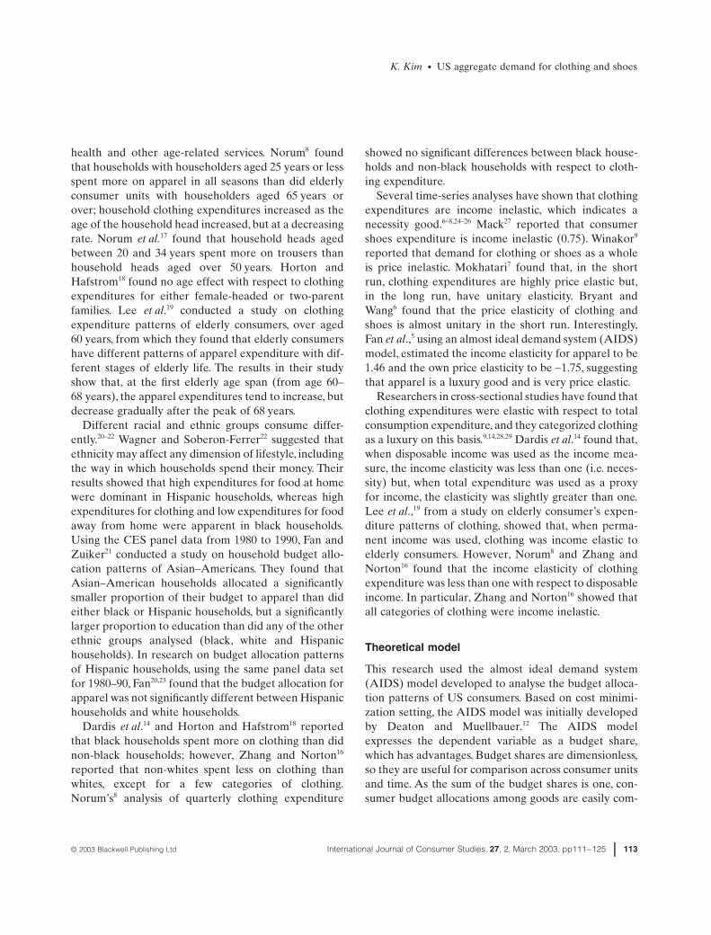
accompanied by increased consumer budget allocationsfor clothing categories and shoes.

Prices

Own pricesThe own price variable represented by the estimated gij

coefficients (i.e. g1WC, g2MB, g3SH and g4ON) appeared to bea significant variable affecting consumer’s budget sharesfor clothing categories and shoes (see Table 2). Thesigns of the own price coefficients were positive forclothing categories and shoes, suggesting that, as theown prices of women’s and children’s clothing, men’sand boys’ clothing and shoes increase, the consumerbudget allocation on each clothing category and shoesincreases. Blanciforti et al.11 also reported a positive signfor the clothing category. The price coefficient repre-sents 100 times the effect on the budget share of a 1%increase in the own price. For example, the non-durablegood budget share for women’s and children’s clothingincreased by 0.0272% with a 1% increase in thewomen’s and children’s clothing price. The value of theestimated coefficient g1WC (0.0272) was the highest,which shows that the women’s and children’s clothingbudget share is the most sensitive to changes in theirown prices.

Cross pricesTable 2 also shows the cross-price effects on each cate-gory. As indicated by the estimated g1SH coefficients, theprice of women’s and children’s clothing was not signif-icantly related to the shoes budget shares (and viceversa). The price of men’s and boys’ clothing repre-sented by the estimated g2SH coefficients is significantlyrelated to the shoes budget shares (and vice versa). Theresult implies that, for example, the budget share forshoes decreases by 0.0099% with a 1% increase in theprice of men’s and boy’s clothing. The price of women’sand children’s clothing, estimated by g1MB coefficients, issignificantly related to the men’s and boys’ clothingbudget shares (and vice versa). The signs of the esti-mated coefficients were positive with the values of0.0134, which implies that the budget share for men’sand boys’ clothing increases by 0.0134% with a 1%increase in the price of women’s and children’s clothing.

The estimated coefficients g1ON, g2ON and g3ON, theprice of other non-durables, is significantly related tothe women’s and children’s clothing, men’s and boys’clothing and shoes budget shares (and vice versa) (seeTable 2). The signs of all the estimated coefficients werenegative, implying that the budget shares of the clothingcategories and shoes decreased with an increase in theprice of other non-durables. The value of the estimatedg1ON coefficient was the highest among the clothing cat-egories and shoes, suggesting that the budget allocationfor women’s and children’s clothing is the most sensitiveto changes in the price of other non-durables. Table 2also shows that the women’s and children’s clothingbudget share decreases by 0.0409% with a 1% increasein the price of other non-durables.

Demographic variables

Median ageThe estimated d1j coefficients (i.e. d1WC, d1MB and d1SH),the median age variable, had a significant effect on thebudget shares for men’s and boys’ clothing and shoes(see Table 2). The US aggregate non-durables budget(ANB) shares for men’s and boys’ clothing and shoesincrease as the median age of the population increases,but the effect on the ANB for women’s and children’sclothing was not statistically significant. The resultsobtained, except in the case of women’s and children’sclothing, support the findings and inferences of Fanet al.’s study5 in which they used the 1980–90 CES dataset, although their research is not exactly comparablewith the present study. The findings from Fan et al.5

using the AIDS model suggested that age has a positiverelationship with apparel budget shares.

Variance in the age distribution of the US populationThe estimated d3j coefficients (i.e. d3WC, d3MB and d3SH)in Table 2 show that the effects of the variance on theANB shares for all categories were not statistically sig-nificant. Thus, the result implies that changes in therelative number of people in the median age group inthe US population have not affected the ANB sharesfor the clothing categories and shoes during the obser-vation period. The signs of estimated d3j coefficientswere positive, except for d3WC.



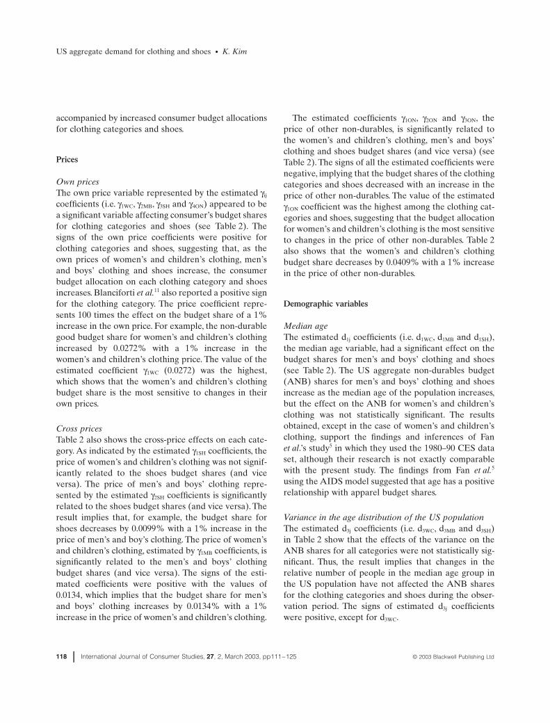
Non-white proportionAs indicated by the estimated d2j coefficients (i.e. d2WC,d2MB and d2SH), the relationships between the proportionof non-white population and the ANB for the clothingcategories and shoes were positive (see Table 2). Theeffect on the ANB for women’s and children’s clothingwas not statistically significant. The effect on the ANBshare for men’s and boys’ clothing was the highestamong the clothing categories and shoes, and the effecton the ANB share for women’s and children’s clothingwas the lowest.

The results suggest that increased consumptionexpenditure allocations to clothing categories and shoesin the US occur as the population of non-whitesincreases. It is also possible to infer from the findingsthat non-whites allocate their expenditure budgetsmore to clothing categories and shoes than whites.

World War IIAs indicated by the estimated kj coefficients (i.e. kWC,kMB and kSH), the dummy variable for World War II wassignificantly related to the ANB shares for women’s andchildren’s clothing and men’s and boys’ clothing, but notto the ANB for shoes, which showed a negative sign (seeTable 2). The findings imply that World War II signifi-cantly influenced the ANB shares for women’s and chil-dren’s clothing and men’s and boys’ clothing.

Demand elasticity

Expenditure and price elasticitiesTable 3 presents estimated demand elasticities withrespect to total non-durables expenditure, price andthe demographic variables. Mean prices and budgetshares were used in calculating the elasticities. The totalnon-durables expenditure elasticities of demands forwomen’s and children’s clothing (WC), men’s and boys’clothing (MB) and shoes (SH) are 1.1695, 1.1019 and1.1157 respectively. All the elasticities have positivesigns, and the categories are expenditure elastic. Theresults suggest that the clothing categories and shoes areluxury goods, and that other non-durable goods (ON)are a necessity. A 10% increase, for example, in totalnon-durable expenditures increases the quantitydemanded for WC by 11.69%.

The own price elasticities are shown on the diagonalsloping downwards to the right in the price elasticitiessection of Table 3. All the own price elasticities ofdemands for the clothing categories and shoes werenegative. The negative signs are consistent with eco-nomic theory for demand; that is, when the prices ofgoods increase, the quantities of the goods demandedgenerally decrease. When the own prices of WC, MBand SH increased, the demand for those categoriesdecreased. The estimated own price elasticities indicatethat the clothing categories and shoes are price inelas-tic. For example, a 10% increase in WC price decreasesWC demand by about 7.4%. MB has the highest ownprice elasticity among the clothing categories andshoes.

The cross-price elasticity of WC demand with respectto MB price has a positive sign, implying a substitute,and it indicates that a 10% increase in MB priceincreases WC demand by 1.24%. The cross-price elas-ticity of MB demand with respect to WC price also hasa positive sign, implying substitutes, but the price effectof WC on MB demand was a little higher than that ofMB on WC demand (i.e. 0.2219 vs. 0.1248). The cross-price effects between WC and MB are both significantlydifferent from zero. Table 3 also shows that the cross-price effects of SH and ON on WC demand are nega-tive, implying complements, which indicate that anincrease in SH or ON price decreases consumers’demand for WC. But the effect of shoes price on WCdemand is not significant. If the price of ON increases10%, the demand for WC decreases by 5.46%. Thecross-price effects of SH and ON on MB demand arealso negative, implying complements, but the effects arerelatively higher than those on WC. The estimated elas-ticities of demand for SH with respect to the prices ofWC, MB and ON are also negative, implying comple-ments, but the effect of WC price is not significantlydifferent from zero.

The results of the estimation of own price elasticitiesindicate that the elasticity of demand for MB was thehighest among the clothing categories and shoes; that is,the MB demand is the most highly responsive to its ownprice change. Only between WC and MB are the cross-price elasticities positive signs, implying substitutes. Theeffect of ON price is the highest in the case of WCdemand. The cross-price effects are low in most cases;



that is, a price increase in one good generally has littleimpact on demands for all other goods.

Demographic elasticitiesTable 3 shows that the effect of the median age of theUS population on the demand for WC was positive. Onthe other hand, the effects of the median age on MBand SH were negative. The effects, however, are notstatistically significant for any of the categories. Allthe effects of the variance in the age distribution on theclothing categories and shoes were negative, and theeffect was highest in shoes. The effect on WC is notstatistically significant. The results of the estimated elas-ticities imply that the demands for clothing categoriesand shoes decrease as the relative number of people inthe median age group decreases, but the demand for

ON increases. An increase in the non-white proportionin the US population has a relatively small impact onthe demand for WC and MB in comparison with theimpact on SH demand. The effects on WC and MB,however, are not significantly different from zero.The result implies that, as the number of non-whitesincreases, the demand for the clothing category andshoes decreases. The estimated elasticities indicate thata 10% increase in the non-white proportion decreasesthe quantity demanded for SH by 6.54%.

Conclusions and implications

This study has presented the parameter estimates forthe budget shares for clothing categories and shoes.First, it can be concluded that total expenditures for

Table 3 Estimated elasticities with respect to total expenditure, prices and demographics

Price elasticities

Expenditure elasticitiesWC MB SH ON

WC -0.7443* 0.1248* -0.0030 -0.5466* 1.1695*(0.0545) (0.0274) (0.0291) (0.0780) (0.0608)

MB 0.2219* -0.8025* -0.1738* -0.3472* 1.1019*(0.0463) (0.0719) (0.0815) (0.0682) (0.0389)

SH -0.0047 -0.3369* -0.3908** -0.3828* 1.1157*(0.0977) (0.1574) (0.2270) (0.1237) (0.0505)

ON -0.0472* -0.0170* -0.0097** -0.8935* 0.9675*(0.0097) (0.0051) (0.0049) (0.0144) (0.0115)

Demographic elasticities

Age NW VA

WC 0.0736 -0.0132 -0.0226(0.2246) (0.2050) (0.1492)

MB -0.2859 -0.0114 -0.8075*(0.1892) (0.1676) (0.1649)

SH -0.1656 -0.6549* -1.4455*(0.3733) (0.2715) (0.3608)

ON 0.0174 0.0266 0.1140*(0.0426) (0.0383) (0.0287)

* P < 0.05; ** P < 0.1.WC, women’s and children’s clothing; MB, men’s and boys’ clothing; SH, shoes; ON, other non-durable goods; Age, median age of US population; VA, variance of the age distribution of the US population; NW, proportion of non-white population of the US.Standard errors are in parentheses. Mean prices and budget shares were used in calculating the elasticities.



non-durables are significant variables that affect con-sumers’ budget allocations for the clothing categoriesand shoes. The expenditure elasticities evaluated for theclothing categories and shoes indicate that US consum-ers are sensitive to changes in total non-durable expen-ditures and that women’s and children’s clothing (WC),men’s and boys’ clothing (MB) and shoes (SH) are lux-ury goods. The demand for the clothing categories andshoes change proportionately more than the total non-durable expenditures. The findings of the study also sug-gest that consumer non-durables budget shares for theclothing categories and shoes will grow at faster ratethan consumer’s real total non-durable expenditures,ceteris paribus, if the real total non-durable expendi-tures increase.

Most own and cross prices also appeared to be signif-icant variables in determining the consumer budgetallocations for the clothing categories and shoes. Theprice of other non-durable goods has a significantimpact on the clothing categories and shoes budgetshare. All the own price elasticities estimated for cloth-ing categories and shoes were less than one (i.e.|elasticity| < 1), which implies that consumer demandfor those categories changes by a smaller proportionthan prices. If the clothing categories and shoes hadbeen more disaggregated for the study, the own priceeffects might be higher than those estimated because, ifa good has many substitutes, that good tends to havehigher price elasticity.

The estimated cross-price elasticities in this studyshowed an interesting fact that the increased price ofwomen’s and children’s clothing or men’s and boys’clothing results in a decrease in the quantitiesdemanded for shoes, implying complementary relation-ships between the clothing categories and shoes. Thecross-price elasticities estimated between the clothingcategories and other non-durable goods and betweenshoes and other non-durable goods show similarchanges, complementary relationships, as in the demandpattern of the cross-price effects between the clothingcategories and shoes. Women’s and children’s clothingdemand is the most sensitive to change in the price ofother non-durable goods among the clothing categoriesand shoes. The results of the cross-price elasticitiesbetween women’s and children’s clothing and men’s andboys’ clothing show substitution relationships, that is

demand for women’s and children’s clothing increaseswith an increase in men’s and boys’ clothing price, andvice versa. The possible explanation for substitutionrelationships may lie in family clothing consumptionbehaviour. Families allocate their budgets not onlyamong clothing and other consumer goods, but alsoamong individual family members and different cloth-ing categories,16 and this family budget allocation andconsumption process is completed via family utilitymaximization.51 Thus, if the market price of women’sand children’s clothing increases, decision makers infamilies may decide to reduce purchases of these itemsand increase purchases of other clothing categories,such as men’s and boys clothing, maintaining the maxi-mum family utility.

The older the population, the more non-durableexpenditures are allocated to men’s and boys’ clothingand shoes. Although the median age of the US popula-tion has increased, from 29.8 years in 1930 to 34 yearsin 1994,4 the median age is still in the range whereclothing expenditures are higher than for the elderly.Thus, the ANB shares for men’s and boys’ clothing andshoes may increase continuously until the median agereaches middle age, 45–54 years, at which point incomeand overall spending peak.52 The median age of the USpopulation was a significant variable that affects USaggregate non-durable expenditures allocation onmen’s and boy’s clothing categories and shoes. The find-ings on the combination of the parameter estimates andthe elasticities estimated suggest that, although the USaggregate non-durables budget (ANB) shares for men’sand boys’ clothing and shoes increases, demand forthese categories decreases as the median age increases.Demand for women’s and children’s clothing, however,increases as the median age increases, but the effect isvery weak. The variance in the age distribution was usedin the model as a proxy variable of population changewith the idea that it would provide information aboutthe effect of the changes in the relative number ofmedian age people on aggregate clothing categories andshoes consumption. In this study, the variance in the USpopulation distribution appeared not to be an importantvariable in determining the change in the US ANBshares for clothing categories and shoes. This may bebecause of lack of variation in the variable or mis-specification in capturing distribution change as well as



the skewness variable. Thus, different measurementmethods for the age group 25–34 years or for the elderlypopulation, such as proportion, are suggested for futurestudies.

In this model estimation, the non-white populationproportion was a significant variable in determining thechange in the US ANB shares for men’s and boys’ cloth-ing and shoes. With an increase in the non-white popu-lation, the US ANB shares for clothing categories andshoes increased. Possible explanations for the findingsmay lie in values and behaviours of racial and ethnicgroups. Gans (cited in Wagner and Soberon-Ferrer22)pointed out that clothing and food are two categories ofgoods that are thought to carry symbolic meaningamong ethnic groups. Although Hispanics are of mixedrace and blacks constitute the largest proportion of theUS non-white group in the present study, Hispanics area major component of non-whites. Hispanics seem tobe oriented towards expressive consumption and to beconcerned with status,53 which are some of the valuesoften expressed in clothing consumption.54 Hispanicsmay spend more than whites on clothing if theyview the consumption of clothing as showing expres-siveness and status. Values of blacks include effect,communalism and expressive individualism,55 which aresimilar to values expressed in clothing consumption.54

Yankelovitch56 reported that blacks are much moreinterested in physical appearance, individuality and cre-ativity than other ethnic groups. Various authors57–59

have noted that blacks use clothing to aid status sym-bolization. Dalrymple et al.60 suggested that blacks aremore likely to purchase new clothing than whites. Thus,if blacks consider clothing consumption as reflectingthose values, they may spend more than whites on cloth-ing. In summary, the age of the population and thenon-white population proportion are significant demo-graphic variables in influencing changes in the US ANBshares for the clothing categories and shoes in the US.The median age of the US population is expected toreach 38.9 years in 2010.38,39 Thus, from the findings ofthis study, it can be predicted that the US ANB sharesfor clothing and shoes will increase until the earlytwenty-first century, ceteris paribus. Whites who are notof Hispanic origin were 75.7% of the population in1990, but this proportion will decrease steadily to 67.6%in 2010;1 thus, ceteris paribus, the US ANB shares for

men’s and boys’ clothing and shoes will increase withthe increased proportion of non-whites by the year2010.

Despite the various efforts of the Office of PriceAdministration to control the price of clothing catego-ries, clothing was the most difficult and least successfulin price control during World War II.44 The price ofclothing was very high, and US consumers spent largerproportions of their consumption expenditures onclothing during wartime in comparison with other peri-ods. Thus, it is believed that World War II stronglyimpacted on the level of consumer budget shares forclothing.

The results of this study may be useful for producersand marketers in the clothing and retail industries. Inthe present study, several economic and demographicvariables related to clothing and shoes consumptionwere explored. Such variables are generally identifiedas macro-environmental factors in establishing market-ing strategy and planning. By understanding the effectsof these variables, the producers and marketers candevelop better marketing strategies for their productlines. For example, when planning to market clothingmerchandise in an area where the proportion of thenon-white population is rising relatively rapidly, such asin some metropolitan areas, the information about thenon-white population obtained from this study can bevaluable in developing long-term marketing plan. Firmsmay wish to adjust their marketing mix variables. Thecoefficients estimated in the study show that consumer’sbudget allocations to men’s and boys’ clothing and toshoes increase as the non-white population increasesand as the prices of these items increase, which may bea good sign of a profitable non-white market in a met-ropolitan area. The estimated elasticity of shoes alsoindicates that consumers’ demand for shoes decreaseswith the increase in the non-white population. Consum-ers will spend more money on shoes but purchase asmaller quantity of shoes in the market with an increas-ing non-white population. Thus, if shoe manufacturersconsider quality as well as price and adjustment of theother marketing mix variables, the market would beprofitable.

There exist limitations of this study. First, each cloth-ing category, shoes and other non-durable goods arehighly aggregated in the study. Future research on more



disaggregated commodity groups is recommended. Sec-ondly, caution should be made against overgeneraliza-tion of the findings in comparison with the results ofother complete demand system analyses because thebudget-share LAIDS model estimated in this study wasconfined to non-durable goods (the total expenditurevariable was total expenditure on non-durable goods).Thirdly, in the study, racial/ethnic groups are separatedinto only two groups (white and non-white), leading tothe assumption that only these two broad groups differin preferences from each other. This assumption, how-ever, may not be realistic. More disaggregated racial/ethnic groups, such as Hispanic, black, Asian and white,are suggested for future time-series studies of consump-tion associated with race/ethnicity because a differentracial/ethnic group may have a different preferencestructure. Another thing that should be mentioned isother ways of measuring age distribution. In the presentstudy, the research used three different central moments(median, variance and skewness), but the second andthird moments (variance and skewness) could not prop-erly capture the variation in the age distribution. Thus,other measuring units are suggested.

References

1. Day, J.C. (1992) Population Projections of the United States, by Age, Sex, Race, and Hispanic Origin: 1992–2050. Current Population Reports. US Bureau of the Census, Series P25-1092. US Government Printing Office, Washington, DC.

2. US Department of Commerce, Bureau of Economic Analysis (1992) The National Income and Product Accounts of the United States: 1959–1988. US Government Printing Office, Washington, DC.


4. US Department of Commerce, Bureau of Economic Analysis (1995) The National Income and Product Accounts of the United States: 1985–1992, 1993–94. US Government Printing Office, Washington, DC.

5. Fan, X.J., Lee, J. & Hanna, S. (1996) Household expenditures on apparel: a complete demand system approach. In Proceedings of American Council on Consumer Interests, Vol. 42 (Ed. by T. Mauldin),

pp. 173–180. American Council on Consumer Interests, Columbia, MO.

6. Bryant, W.K. & Wang, Y. (1990) American consumption patterns and the price of time: a time-series analysis. Journal of Consumer Affairs, 24, 280–306.

7. Mokhatari, M. (1992) An alternative model of US clothing expenditures: application of cointegration techniques. Journal of Consumer Affairs, 26, 305–323.

8. Norum, P.S. (1989) Economic analysis of quarterly household expenditures on apparel. Home Economics Research Journal, 17, 228–240.

9. Winakor, G. (1989) The decline in expenditures for clothing relative to total consumer spending, 1929–86. Home Economics Research Journal, 17, 195–215.

10. Houthakker, H.S. & Taylor, L.D. (1970) Consumer Demand in the United States: Analyses and Projections. Harvard University Press, Cambridge, MA.

11. Blanciforti, L., Green, R.D. & King, G.A. (1986) US Consumer Behavior over The Postwar Period: An Almost Ideal Demand System Analysis. Giannini Foundation Monograph no. 40. Division of Agriculture and Natural Resources, California Agricultural Experiment Station, University of California.

12. Deaton, A. & Muellbauer, J. (1980) An almost ideal demand system. American Economic Review, 70, 312–326.

13. Magrabi, F.M., Chung, Y.S., Cha, S.S. & Yang, S. (1990) The Economics of Household Consumption. Praeger Publications, New York.

14. Dardis, R., Derrick, F. & Lehfeld, A. (1981) Clothing demand in the United States: a cross-sectional analysis. Home Economics Research Journal, 10, 212–221.

15. Hager, C.J. & Bryant, W.K. (1977) Clothing expenditures of low-income rural families. Journal of Consumer Affairs, 11, 127–132.

16. Zhang, Z. & Norton, M.J.T. (1995) Family members’ expenditures for clothing categories. Family and Consumer Sciences Research Journal, 23, 311–336.

17. Norum, P.S., Weagley, R.O. & Norton, M.J.T. (1998) The effects of uniforms on nonuniform apparel expenditures. Family and Consumer Sciences Research Journal, 26, 259–280.

18. Horton, S.E. & Hafstrom, J.L. (1985) Income elasticities for selected consumption categories: comparison of single female-headed and two-parents families. Home Economics Research Journal, 13, 292–303.

19. Lee, J., Hanna, S.D., Mok, C.F.J. & Wang, H. (1997) Apparel expenditure patters of elderly consumers: a life-cycle consumption model. Family and Consumer Sciences Research Journal, 26, 109–140.



20. Fan, X.J. (1994) Household budget allocation patterns of Asia-Americans: are they different from other ethnic groups? In Proceedings of American Council on Consumer Interests, Vol. 40 (Ed. by T. Mauldin), pp. 81–88. American Council on Consumer Interests, Columbia, MO.

21. Fan, X.J. & Zuiker, V.S. (1994) Budget allocation patterns of hispanic versus non-hispanic white households. In Proceedings of American Council on Consumer Interests, Vol. 40 (Ed. by T. Mauldin), pp. 89–96. American Council on Consumer Interests, Columbia, MO.

22. Wagner, J. & Soberon-Ferrer, H. (1990) The effect of ethnicity on selected household expenditures. Social Science Journal, 27, 181–198.

23. Fan, X.J. (1997) Expenditure patterns of Asian Americans: evidence from the US consumer expenditure survey, 1980–92. Family and Consumer Science Research Journal, 25, 339–368.

24. Eastwood, D.B. & Craven, J.A. (1981) Food demand and savings in a complete, extended, linear expenditure system. American Journal of Agricultural Economics, 63, 544–549.

25. Hamburg, M. (1960) Demand for clothing. Study of consumer expenditures, incomes, and savings. In Proceedings of the Conference on Consumption and Saving (Ed. by I. Friend & R. Jones), pp. 311–358. University of Pennsylvania, Philadelphia, PA.

26. Jackson, K.C. & Al-Douri, S.M. (1977) The demand for clothing: an econometric analysis. Clothing Research Journal, 5, 129–138.

27. Mack, R.P. (1954) Factors Influencing Consumption: An Experimental Analysis of Shoe Buying. National Bureau of Economic Research, New York.

28. Winakor, G. (1962) Consumer expenditures for clothing in the United States, 1929–58. Journal of Home Economics, 54, 115–118.

29. Nelson, J.A. (1989) Individual consumption within the household: a study of expenditures on clothing. Journal of Consumer Affairs, 23, 21–43.

30. Moschini, G. (1995) Units measurement and the Stone index in demand system estimation. American Journal of Agricultural Economics, 77, 63–68.

31. Buse, A. (1994) Evaluating the linearized almost ideal demand system. American Journal of Agricultural Economics, 76, 781–793.


33. Deaton, A. & Muellbauer, G. (1993) Economics and Consumer Behavior. Cambridge University Press, New York.

34. US Bureau of the Census (1975) Historical Statistics of the United States: Colonial Times to 1970. Bicentennial Edition, Part 1. US Government Printing Office, Washington, DC.

35. US Bureau of the Census (1992) Statistical Abstract of the United States (112th). US Government Printing Office, Washington, DC.



38. US Bureau of the Census (1988) United States Population Estimates by Age, Sex and Race: 1980–87. Current Population Reports, Series P25-1022. US Government Printing Office, Washington, DC.

39. US Bureau of the Census (1988) United States population Estimates by Age, Sex and Race: 1970–87. Current Population Reports, Series P25-1023. US Government Printing Office, Washington, DC.

40. US Bureau of the Census (1982) Preliminary Estimates of the Population of the USA by Age, Sex and Race: 1970–81. Current Population Reports, Series P25-917. US Government Printing Office, Washington, DC.

41. Ott, R.L. (1993) An Introduction to Statistical Methods and Data Analysis. Duxbury Press, Belmont, CA.

42. Greene, W.H. (1996) Econometric Analysis. Macmillan Publishing, New York.

43. American War Production Board (1942) Federal Register. The National Archives of the US Publication no. 7–69, pp. 2722–2729. American War Production Board, Washington, DC.

44. Harris, S.E. (1976) Price and Related Controls in the United States. Da Capo Press, New York.

45. Polenberg, R. (1972) War and Society. Greenwood Press, Westport, CT.

46. Vatter, H.G. (1985) The US Economy in World War II. Columbia University Press, New York.

47. Rao, C.R. (1973) Linear Statistical Inference and its Applications. John Wiley and Sons, New York.

48. McGuirk, A.M., Driscoll, P., Alwang, J. & Huang, H. (1995) System misspecification testing and structural change in the demand for meats. Journal of Agricultural and Resource Economics, 20, 1–21.

49. Attfield, C.L.F. (1991) Estimation and testing when explanatory variables are endogenous. Journal of Econometrics, 48, 395–408.

50. Hausman, J.A. (1978) Specification tests in econometrics. Econometrica, 46, 1251–1271.



51. Norton, M.J.T. & Park, J.O. (1986) Household demand, expenditures, and budgets for clothing. In College of Human Resources: Research Conference Proceeding (Ed. by M.J. Sporakowski, R.P. Lovinggood, J.A. Driskell & B.E. Densmore), pp. 71–90. Virginia Agricultural Experiment Station, Virginia Polytechnic Institute and State University, Blacksburg, VA.

52. Frances, P. (1995) America at mid-decade. American Demographics, 17 (2), 23–31.

53. Hirschman, E. (1982) Ethnic variation in leisure activities and motives. In American Marketing Association Educators’ Proceedings, pp. 93–98. American Marketing Association, Chicago, IL.

54. Horn, M.J. & Gurel, L.M. (1981) The Second Skin. Houghton, New York.

55. Boykin, A.W. (1983) The academic performance of Afro-American children. In Achievement and Achievement

Motives: Psychological and Sociological Approaches (Ed. by J.T. Spence), pp. 325–371. W.H. Freeman, New York.

56. Yankelovitch, D. (1973) A new look at the Black consumer. Sales Management, August, 13.

57. Bauer, R.A. & Cunningham, S.A. (1970) The Negro market. Journal of Advertising Research, 10 (2), 3–13.

58. Johnson, R.C. (1981) The black family and black community development. Journal of Black Psychology, 8, 23–39.

59. Swartz, J. (1963) Men’s clothing and the Negro. Phylon, 24, 230.

60. Dalrymple, D.J., Robertson, T. & Yoshino, M. (1971) Consumer behavior across ethnic categories. California Management Review, 14, 65–70.

Documents

US aggregate demand for clothing and shoes: effects of non-durable expenditures, price and demographic changes