This PDF is a selection from an out-of-print volume from the National Bureauof Economic Research

Volume Title: Determinants of Investment Behavior

Volume Author/Editor: Robert Ferber, editor

Volume Publisher: NBER

Volume ISBN: 0-87014-309-3

Volume URL: http://www.nber.org/books/ferb67-1

Publication Date: 1967

Chapter Title: Consumer Expenditures for Durable Goods

Chapter Author: Marvin Snowbarger, Daniel B. Suits

Chapter URL: http://www.nber.org/chapters/c1240

Chapter pages in book: (p. 333 - 355)

Consumer Expenditures

for Durable Goods

MARVIN SNOWBARGER AND DANIEL B. SUITSUNIVERSITY OF MICHIGAN

This paper presents the findings of research on the demand for consumerdurables, using cross-sectional data from the Survey of ConsumerFinances. The annual surveys, conducted by the Survey ResearchCenter at the University of Michigan, of 1960, 1961, and 1962 con-tained a reinterview (panel) sample of 1059 households.' The data areanalyzed by the Sonquist-Morgan Automatic Interaction Detector(AID) program,2 developed for the IBM 7090 computer. Essentially,this is a method for searching a large body of data for important rela-tionships. It differs from most research procedures in that it seeks outthe most important variables without having them prespecified. The pro-gram is discussed in section I.

Section II presents an application of the AID program to consumerinvestment decisions. The program is used to examine the characteristicsthat distinguished households who subsequently buy a specific durablefrom those that do not. The individual durables studied are televisionsets, refrigerators, washers, furniture, and automobiles.

Since automobiles are the major component of consumer durableexpenditure, the phenomenon of the two-car family has special implica-tions for the industry and the national economy. In section III, the pro-gram is used to study multiple-car ownership.

1 The 1960—62 panel and its characteristics are discussed in R. Kosobud andJ. Morgan, Consumer Behavior of Individual Families over Two and Three Years,Survey Research Center, 1964.

2 John Sonquist and James Morgan, The Detection of Interaction Eflects, Mono-graph No. 35, Survey Research Center, 1964.

334 Consumer Assets

I. The Method of AnalysisRegression and related techniques are often used to analyze cross-sectiondata, but the diversity of individual consumer behavior and the complexintercorrelations and interactions preclude a straightforward linearregression. Cross tabulations often provide a better proffle of consumerbehavior, but still require the analyst to select the "control" variablesin advance. As a practical matter, however, he rarely knows all theimportant variables, especially where complex interactions are involved.The Automatic Interaction Detector (AID) program provides an alter-native by which the data can be scanned to identify the most importantvariables and their interactions.

The program is essentially a way of partitioning the total sample ofobservations by a sequence of dichotomies. At each stage the computerattempts to use the variables to divide the existing subsets. Each subsetis partitioned by the variable yielding the maximum R2. The procedureterminates when individual subsets are either sufficiently homogeneousor contain a minimum number of observations. Upon completion, thecomputer output specifies a "tree" of two-way splits, providing a pic-ture of the relationship by defining a series of increasingly complexinteractions.

At each step the program scans several variables, but selects only oneof them. An important feature of the program is its ability to allowevery variable the chance to become a predictor at each stage. In anysplit, some variables may be highly cbrrelated with the partitioningvariable, but not sufficiently powerful to make the split. A highly cor-related variable at one stage may return to partition a group later in thetree. Information about the status of all variables is contained inthe printed output of the program. In particular, the relative discrimi-nating power of each variable is shown at every stage of the program,making it possible to compare the one ultimately chosen with all alter-natives. This contributes to an understanding of why one variableappears rather than another, and how great the difference between themwas. Any interpretation of the tree must be supported by an analysisof the splits that "almost" occurred.

If the program is allowed to run without constraint, it may split offa very small group. These splits must be recognized for their extremevariation, but disregarded in the final analysis.

Each variable appearing in the tree makes a contribution to theexplanation of the dependent variable. Its relative strength is indicatedby a "partial R2." The total of all these "partial R2's" is equal to theproportion of the total variation "explained" by the splits in the tree.

Consumer Expenditures for Durable Goods

TABLE 1

List of Variables Used in Panel Analysis

335

— 1

Variables Code Categories

Dependent G:Whether purchased TVWhether purchased refrigeratorWhether purchased washerWhether purchased furnitureWhether purchased automobile

Purchased;Purchased;Purchased;Purchased;Purchased;

did not purchasedid not purchasedid not purchasedid not purchasedid not purchase

IndependentBetter or worse off than year agoExpect to be better off year from nowSize of placeAge of headNumber of adultsNumber of children under 18Age of youngest child under 18Age of oldest child under 18Marital statusLength of marriageDate residence established

Housing statusWhether head employed nowNumber of weeks head workedNumber of weeks wife workedWife's employment statusAIDPR/disposable incomeDisposable incomePercentage of incomeRemaining instalmentRemaining instalmentRemaining instalmentRemaining instalmentWhether expect to buy TVWhether expect to buy refrigeratorWhether expect to buy washer

expect to buy furnitureWhether expect to buy automobile

Better; same; worse; uncertainBetter; same; worse; uncertainCentral cities; urban places; rural places18-24; 25-34; 35-44; 45-54; 55-64; 65-0; 1; 2; 3; 4; 5; 6; 7; 8 or more0; 1; 2; 3; 4; 5; 6; 7; 8 or more2-3; 3-4; 4-5; 5-6; 6-9; 9-14; 14-182-3; 3-4; 4-5; 5-6; 6-9; 9-14; 14-18Married; single; widow; divorced; separated0-1; 2;. 3; 4; 5-9; 10-20; over 20 yearsPre-1939; 1940-49; 1950-54; 1955-56; 1957;

1958; 1959; 1960Owner; renterEmployed; unemployed; retired13 or less; 14-26; 27-39; 40-47; 48-49; 50-5213 or less; 14-26; 27-39; 40-47; 48-49; 50-52Worked 2 years ago; worked last yearPercentage scaleDollar scalePercentage scaleDollar scaleDollar scaleDollar scaleDollar scaleDefinitely; probably; undecidedDefinitely; probably; undecidedDefinitely; probably; undecidedDefinitely; probably; undecidedDefinitely; probably; undecided

received by wifedebt on A/Rdebt on carsdebt on durablesdebt on other

a These variables are part of the independent variables unless they are the dependent,ariable in a particular run.

Exp

ecte

d to

buy

TV

FIG

UR

E 1

Fact

ors

ted

to P

urch

ase

of a

Tel

evis

ion

Set

Sour

ce: 1

960-

62 S

urve

y of

Con

sum

er F

inan

ces.

N-1

059.

Rat

io o

l deb

tre

pay.

rat

e to

disp

os. i

ncom

e

Rem

aini

ngin

stal

. deb

ton

dur

abte

s

Bou

ght r

ange

No.

of C

hild

ron

unde

r 18

Dis

posa

ble

inco

me

Var

iatio

n ex

plai

ned:

15

per c

ent.

Consumer Expenditures for Durable Goods 337

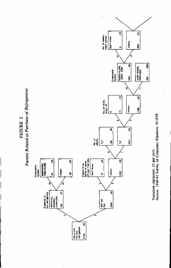
ii. Purchase of DurablesThe AID program is used in this section to study the purchase of con-sumer durables. The Survey of Consumer Finances, conducted by theSurvey Research Center, contains information on the purchase of tele-vision sets, refrigerators, washers, furniture, and automobiles, togetherwith extensive attitudinal, demographic, and economic data. The1960—62 Surveys contained a panel of 1059 households, each of whichwas interviewed three times. Information is available describing theposition of the family at each interview, and its purchase behavior dur-ing the past year. For each durable, the attempt was made to relate thecharacteristics of the family at one interview to its subsequent purchas-ing behavior as determined from the following interview. Since threeinterviews were conducted, two observations were available for eachhousehold. The complete data set used in this analysis consists of 2118observations.

Specifically, the data were arranged in the following way. A particulardurable was selected and the value 1 assigned to a household if it pur-chased the durable between 1960 and 1961. Otherwise, the householdwas assigned the value 0. Corresponding data for the independent vari-ables were compiled as of January 1960. This yields 1059 households,each of which is known either to have purchased or not to have pur-chased the durable between January 1960 and January 1961. All datafor these households were obtained at most one year prior to the actualpurchase.

The procedure was repeated for the same households, but usingpurchase behavior of the period 1961—62. The data for the independentvariables were compiled as of January 1961, yielding an additional 1059observations. All data for these households are, likewise, no later thanone year prior to the actual purchase behavior.

Combining the two groups of data produces the data set of 2118 obser-vations. The several variables used in the study are listed in Table 1.

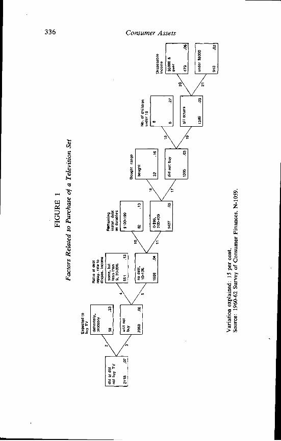
The relationship of the independent variables to the purchase of atelevision set is shown in Figure 1. The first box shows that, of the 2118interviews, 7 per cent were followed by the purchase of a television set.The first branch of the tree shows that "plans to buy a TV" is the mostimportant information distinguishing purchasers from nonpurch asers.Among households with expressed intentions to buy, 33 per centbought, compared with only 6 per cent of those who did not plan to buy.Although two-thirds of families "planning to buy" actually failed to doso, the group was too small to be split again.

FIG

UR

E 2

Var

iatio

n ex

plai

ned:

23

per c

ent.

Sour

ce: 1

960-

62 S

urve

y of

Con

sum

er F

inan

ces.

N-1

059.

Exp

ecte

d to

buy

refr

iger

ator

Fact

ors R

elat

ed to

Pur

chas

e of

Ref

riger

ator

Oia

poaa

bte

inco

me

No.

of

adul

ts

No.

of c

hild

.N

o. o

f wee

ksun

der

18he

ad w

orke

d

Dis

posa

ble

inco

me

FIG

UR

E

Age

of h

ead

2 (c

oncl

uded

)

-t -t -t -S w '0

Hou

sing

sta

tus

14

Mar

ital s

tatu

sE

mpl

oym

ent

stat

us o

f wife

Dat

e re

side

nce

esta

blis

hed

340 Consumer Assets

The next branch of the tree shows the importance of the annualrepayment rate of consumer debt in distinguishing purchasers from non-purchasers.3 Among households expressing no intention to buy, a largenumber of purchases (13 per cent) was made by households whosedebt repayment rate as a percentage of income was either very low orvery high. Fewer purchases are found among households with a moder-ate debt repayment to income ratio. Among the latter, families withmoderate amounts of instalment debt bought television sets.

The final branches of the tree show the influence of "buying a range,"the "number of children under 18," and "disposable income." Neitherthe purchase of a range nor the number of children under 18 provideuseful information. The number of observations in these two splits isthirty-two for the former, and six for the latter. After taking account ofall the other influences, however, disposable income still produces adifference in behavior.

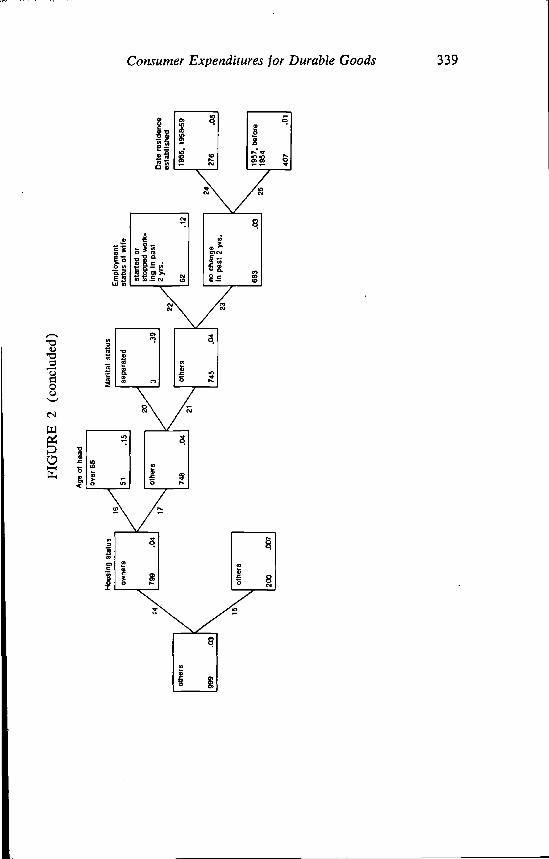
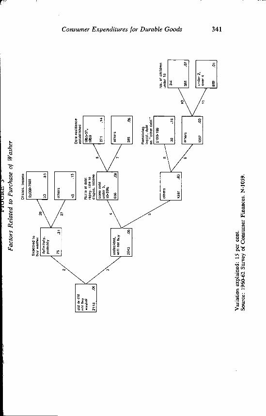
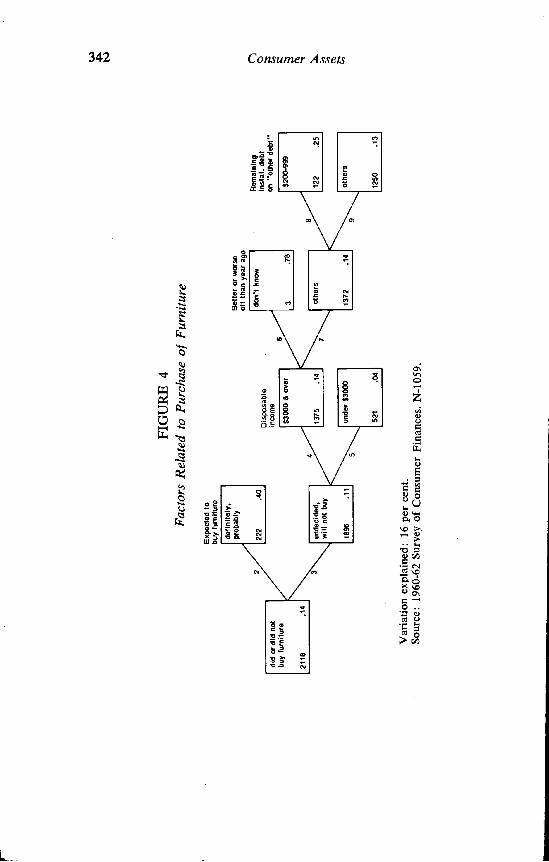
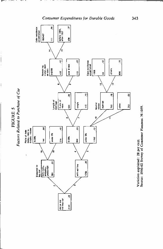
Figure 2 displays the AID tree purchases of a refrigerator. Forty-nine per cent of the households planning to buy, and having income inthe $4,000_$6,000 and $7,500—$10,000 range, actually bought a refrig-erator. The lengthy series of splits on the bottom of the tree shows thatextreme variability, arising for a number of reasons, will produce manysmall partitions. An interpretation must be selective. Splits 7, 10, 14,and 24 highlight the characteristics of households with no prior inten-tions of buying a refrigerator. Households of one or two adults (split 7),with middle to high income (split 10), who are homeowners (split 14),and recently established (split 24), are more likely to buy refrigeratorsthan households without these attributes. Results for washers, furniture,and automobiles are similar and are shown in Figures 3, 4, and 5.

The purchasing behavior shown by the five trees exhibits a number ofimportant common elements. In every case, expressed purchase inten-tions are the first criterion for identifying eventual buyers. Nevertheless,less than half of those households planning to buy will carry out theirintentions. Other characteristics separate buyers from nonbuyers.4 Theseusually include debt position and disposable income. In no case did thetwo general attitudinal variables ("better off than a year ago," "expect

George Katona, The Power/ui Consumer, New York, 1960, pp. 186 if.4 Buying intentions and their fulfillment are discussed in 1962 Survey of Con-

sumer Finances, Survey Research Center, 1963, Ch. 8.

Fact

ors R

elat

ed to

Pur

chas

e of

Was

her

Exp

ecte

d to

buy

was

her

Dis

pos.

inco

me

2

Rat

io o

f deb

tre

pay.

rat

e to

Dat

e re

side

nce

esta

blis

hed

disp

os. i

ncom

e

Rem

aini

ngin

stal

. deb

ton

"ot

her

debt

"

No.

of c

hild

ren

unde

r 18

9

Var

iatio

n ex

plai

ned:

15

per c

ent.

Sour

ce: 1

960-

62 S

urve

y of

Con

sum

er F

inan

ces.

N-1

059.

I.

FIG

UR

E 4

Fact

ors R

elat

ed to

Pur

chas

e of

Fur

nitu

re

Var

iatio

n ex

plai

ned:

16

per c

ent.

Sour

ce: 1

960-

62 S

urve

y of

Con

sum

er F

inan

ces.

N-1

059.

c.)

Exp

ecte

d to

tum

iture

Dis

posa

ble

inco

me

Bet

ter

or w

orse

ott t

han

year

ago

Rem

aini

ngin

stal

. deb

ton

"ot

her

debt

"

n

FIG

UR

E 5

Fact

ors R

elat

ed to

Pur

chas

e of

Car

Rat

ioof

deb

tre

pay.

rat

e to

disp

os. i

ncon

t

Exp

ecte

d to

buy

car

Rem

aini

ngin

stal

. deb

ton

car

s

Leng

th o

fm

arria

ge

Dat

e re

side

nce

esta

blis

hed

Dat

e re

side

nce

esta

bl is

hed

Var

iatio

n ex

plai

ned:

28

per c

ent.

Sour

ce: 1

960-

62 S

urve

y of

Con

sum

er F

inan

ces.

N-1

059.

a

344 Consumer Assets

TABLE 2

Multiple-Car Ownership Among All Spending Units a

Percentage of Spending UnitsYear Owning More Than One Car

1963 18.51962 18.51961 14.31960 14.41959 12.3

1958 11.8

1957 10.4

1956 9.6

1955 8.8

1954 7.6

1953 77

Source: Survey of Consumer Finances.a A spending unit is defined as all related persons

living together who pooi their incomes. Husband, wife,and children under 18 living at home are members ofthe same spending unit.

to be better off a year from now") contribute to an understanding of thespecific purchase behavior.5

The possible complementarity or substitutability of durable purchaseswas studied by including among the independent variables explainingthe purchase behavior with regard to any one good the observed pur-chase behavior with regard to each of the others. For example, inattempting to distinguish buyers of television sets from nonbuyers, theAID program considered whether the household bought, say, an auto-mobile during the same period. If purchases of automobiles and tele-

There is a considerable literature on the role of "buying intentions," "attitudes,"and consumer demand. Substantive issues are represented, in part, by the followingpublications: J. Tobin, "On the Predictive Value of Consumer Intentions and Atti-tudes," Review of Economics and Statistics, February 1959, pp. 1—11; Eva Mueller,"Consumer Attitudes: Their Influence and Forecasting Value," in The Quality andEconomic Significance of Anticipations Data, Princeton for National Bureau ofEconomic Research, 1960, pp. 149—174; Eva Mueller, "Ten Years of AttitudeSurveys: Their Forecasting Record," Journal of the American Statistical Associa-tion, December 1963, pp. 899—917.

Per cent

Consumer Expenditures for Durable Goods 345

FIGURE 6Percentage of Spending Units Owning More Than One Car

and New U.S. Passenger Car Registrations, 1953-63

1953 '54

3

2

Source: Ward's Automotive Yearbook; Survey of Consumer Finances.Note: A spending unit consists of all related persons living together who pooltheir incomes.

vision sets are complementary, we should expect known purchases ofone to be frequently accompanied by purchase of the other. If the twopurchases are substitutes, known purchase of one should be frequentlyaccompanied by failure to purchase the other. In either case, knownpurchase of the one good should show up as a discriminator. The gen-eral failure to do so suggests that the purchases are not generally relatedin either fashion.

The foregoing analysis highlights the vast complexity of consumerbehavior. If we imagine the trees to be employed to predict the behaviorof families, it is clear that, regardless of our information, the best bet isthat any given family will not purchase the durable in question. Therare exceptions are those like the subsample of families who both expectto purchase a washer and whose income is in the $5,000—$7,500 bracket.Since 55 per cent of such families went on to buy a washer, the odds

2(

M II Lo n S

8

lb

/ \ New-car/ _,/ ///\

1(

7

6

5

4

Multi-car ownershipC.— scale)

0'56 '57

I

346 Consumer Assets

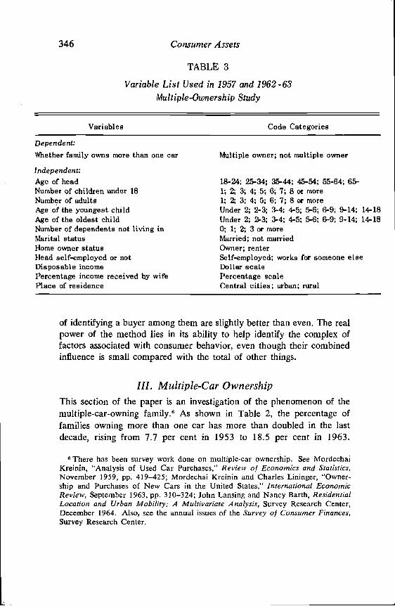
TABLE 3

Variable List Used in 1957 and 1962 -63Multiple-Ownership Study

Variables

Dependent:Whether family owns more than one car

Independent:Age of headNumber of children under 18Number of adultsAge of the youngest childAge of the oldest childNumber of dependents not living inMarital statusHome owner statusHead self-employed or notDisposable incomePercentage income received by wifePlace of residence

Code Categories

Multiple owner; not multiple owner

18-24; 25-34; 35-44; 45-54; 55-64; 65-1; 2; 3; 4; 5; 6; 7; 8 or more1; 2; 3; 4; 5; 6; 7; 8 or moreUnder 2; 2-3; 3-4; 4-5; 5-6; 6-9; 9-14; 14-18Under 2; 2-3; 3-4; 4-5; 5-6; 6-9; 9-14; 14-180; 1; 2; 3 or moreMarried; not marriedOwner; renterSelf-employed; works for someone elseDollar scalePercentage scaleCentral cities; urban; rural

of identifying a buyer among them are slightly better than even. The realpower of the method lies in its ability to help identify the complex offactors associated with consumer behavior, even though their combinedinfluence is small compared with the total of other things.

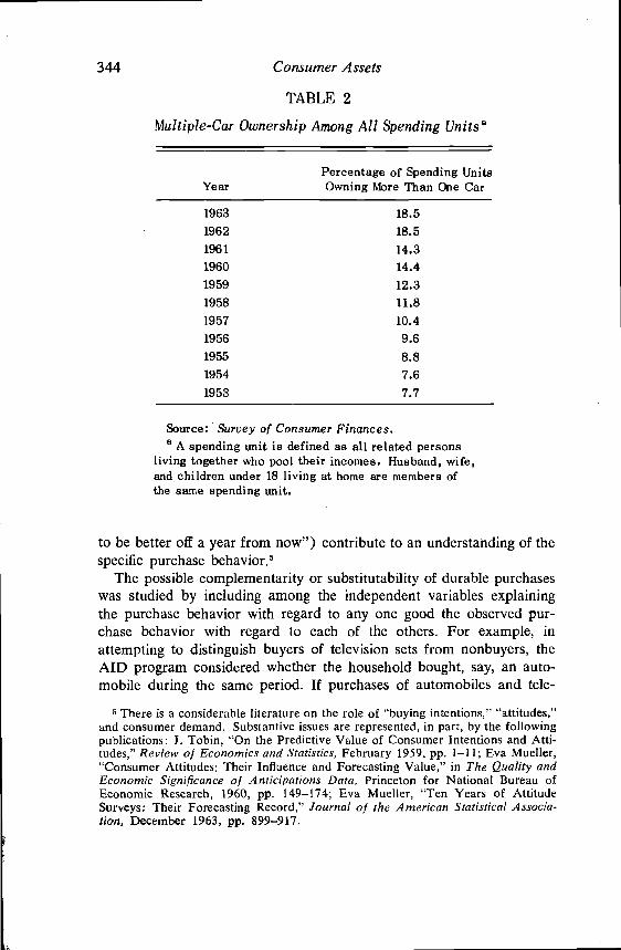
III. Multiple-Car OwnershipThis section of the paper is an investigation of the phenomenon of themultiple-car-owning family.6 As shown in Table 2, the percentage offamilies owning more than one car has more than doubled in the lastdecade, rising from 7.7 per cent in 1953 to 18.5 per cent in 1963.

6 There has been survey work done on multiple-car ownership. See MordechaiKreinin, "Analysis of Used Car Purchases," Review of Economics and Statistics,November 1959, pp. 419—425; Mordechai Kreinin and Charles Lininger, "Owner-ship and Purchases of New Cars in the United States," International EconomicReview, September 1963, pp. 3 10—324; John Lansing and Nancy Barth, ResidentialLocation and Urban Mobility: A Multivariate Analysis, Survey Research Center,December 1964. Also, see the annual issues of the Survey of Consumer Finances,Survey Research Center.

FIG

UR

E 7

Cro

ss-S

ectio

nal C

hara

cter

istic

s of M

ultip

le-C

ar O

wne

rshi

p, 1

957

(non

owne

rs e

xclu

ded)

Var

iatio

n ex

plai

ned:

27

per c

ent.

Sour

ce: 1

957

Surv

ey o

f Con

sum

er F

inan

ces.

N-3

041.

DIS

PO

S. i

ncom

e

No.

of a

dults

Ois

pos.

inco

me

Hom

e-ow

ner

slat

uS

Res

iden

ce

Age

of o

ldes

tch

ild u

nder

18

No.

of a

dults

% o

f inc

ome

earn

ed b

y w

ife

Var

iatio

n ex

plai

ned:

35

per

cent

.So

urce

: 196

2-63

Sur

vey

of C

onsu

mer

Fin

ance

s. N

(19&

2)-2

117.

N (1

963)

-203

6.

FIG

UR

E 8

Cro

ss-S

ectio

nal C

hara

cter

istic

s of M

ultip

le-C

ar O

wne

rshi

p, 1

962-

63(n

onow

ners

exc

lude

d)

Dis

pos.

Inco

me

Age

of y

oung

est

child

und

er 1

8

9-18

163

.64

I oth

ers

172

.39

Res

iden

ce

rura

l

398

.37

112

larg

est

Imet

ropo

l.

Age

of y

oung

est

child

und

er 1

8

.21

Age

of o

ides

tch

ild u

nder

18

10-1

2, 1

4, 1

7

Age

of h

ead

Age

of y

oung

est

chIld

und

er 1

8

Consumer Expenditures for Durable Goods 349

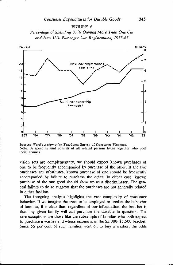
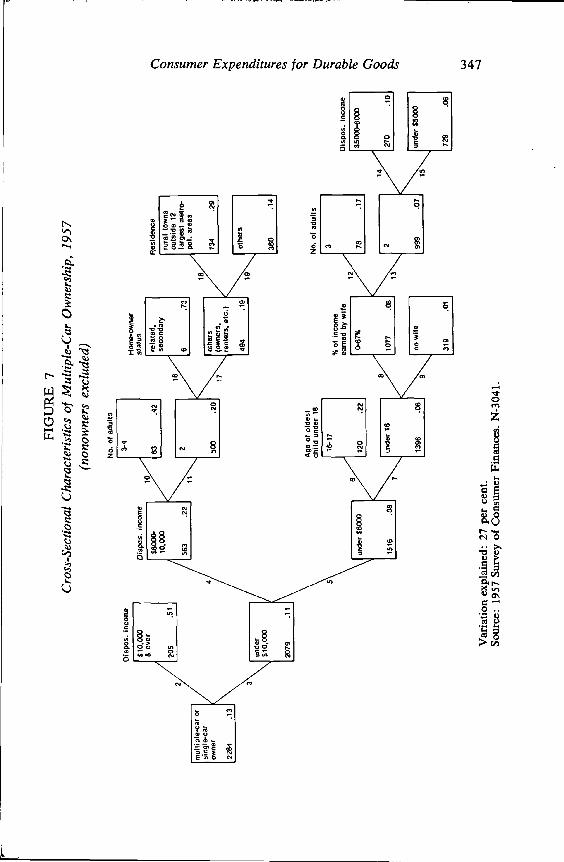
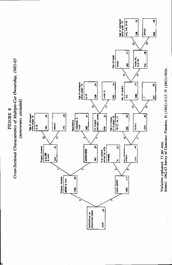
Figure 6 shows the growth in multiple-car-owning families in relation tototal new automobile demand.

AID runs were designed to study the cross-sectional characteristics ofmultiple-car-owning families. The data are from the 1957 Survey ofConsumer Finances and the 1962 and 1963 Surveys of ConsumerFinances. One AID run was made on the 1957 data. Another, withidentical variables, was made on the 1962—63 data. The list of variablesis given in Table 3. The runs were designed to study multiple owner-ship among car owners. Therefore, all households that did not owncars (i.e., nonowners) have been excluded from these two runs. The1957 multiple ownership AID run is in Figure 7. The 1962—63 AIDrun is in Figure 8.

Both the 1957 and the 1962—63 trees separate households into threeincome groups: under $6,000, $6,000—$10,000, and $10,000 and over.

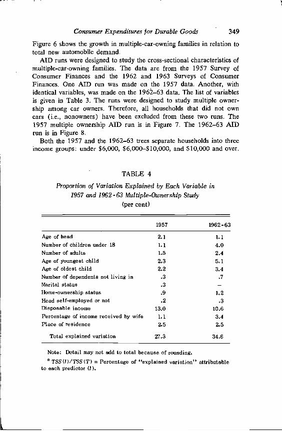
TABLE 4

Pro portion of Variation Explained by Each Variable in1957 and 1962 -63 Multiple-Ownership Study

(per cent)

1957 1962-63

Age of head 2.1 1.1Number of children under 18 1.1 4.0Number of adults 1.5 2.4Age of youngest child 2.3 5.1Age of oldest child 2.2 3.4Number of dependents not living in .3 .7Marital status .3Home-ownership status .9 1.2Head self-employed or not .2 .3Disposable income 13.0 106Percentage of income received by wife Li 3,4Place of residence 2.5

Total explained variation 27.3 34.6

Note: Detail may not add to total because of rounding.a TSS(I)/TSS(T) = Percentage of "explained variation" attributable

to each predictor (I).

Var

iatio

n ex

plai

ned:

71

per c

ent.

Sour

ce: 1

957

Surv

ey o

f Con

sum

er F

inan

ces.

N-3

041.

UI 0

FIG

UR

E 9

Cro

ss-S

ectio

nal C

hara

cter

istic

s of M

ultip

le-C

ar O

wne

rshi

p, 1

957

(sin

gle-

car o

wne

rs e

xclu

ded)

Hea

d se

lf-em

pld.

or w

orks

for

som

eone

els

e

Res

iden

ce

Dis

pos.

inco

me

Inco

me

Consumer Expenditures for Durable Goods 351

FIGURE 10Cross-Sectional Characteristics of Multiple-Car Ownership, 1962-63

(single-car owners excluded)HOme.owne,shipstatus

Multiple ownership among low-income families in 1957 is stronglyinfluenced by older children and working wives. The impact of olderchildren is the only major influence on low-income families in 1962—63.

Multiple-car ownership among middle-income families is explainedby place of residence in both periods. Disregarding the minor splits in1957, urban cities outside the twelve largest metropolitan areas andrural towns are the best discriminators. Middle-income households inthe central cities are unlikely to be multiple owners. The pattern appearsto be stable between 1957 and 1962—63.

Among upper-income groups, the age of older children is importantin the 1962—63 tree. The upper-income group is not split in 1957.

The broad characteristics of the AID trees in these two periods areprimarily captured by the division of multiple owners into three distinctincome classes. In addition, the discriminating features of the threegroups are somewhat different. Residence seems to influence middle-income families more than either of the two other income groups, but

No. ofadults

Dlspos. Income

Variation explained: 74 per cent.Source: 1962-63 Survey of Consumer Finances. N (1962)-2117. N (1963)-2036.

352 Consumer Assets

the impact of children, especially in the teen-age groups, appears in vari-ous guises in all income groups. In the 1957 tree, only low-incomemultiple owners were characterized by children in certain age groups.By 1962—63, the influence of older children was diffused throughout theseparate income groups. One way or another, the variables explainingmultiple ownership in terms of family composition were more importantin 1962—63.

Table 4 shows the partial R2's, calculated from the two AID trees.These statistics show the relative strength of the variables. A comparisonof the variables over time indicates their changing importance. Whiledisposable income is seen to be the single most important factor, itdeclined in importance between 1957 and 1962—63. The combined setof variables measuring the number and ages of children under 18 ranksecond to income, and have risen in importance. The wife's contribu-tion to household income has also become more important in dis-tinguishing two-car owners.

As a supplement to the analysis of the distinction between single- andmultiple-car owners, it is useful to explore the distinction betweenmultiple-car owners and those households with no car at all. Again,AID trees were created for the two periods, 1957 and 1962—63, withthe dependent variable being ownership of more than one car or of nocars. The variables and data were identical to those used in the runsdescribed above. The resulting trees are in Figures 9 and 10.

The remarkable feature of these two trees is the amount of variationexplained by the selected predictors: 71 per cent of the variation isexplained in 1957, and 74 per cent in 1962—63, percentages that areextremely high for survey data.

Both trees show that approximately 20 per cent of low-incomefamilies with working wives are multiple-car owners. There is virtuallyno multiple-car ownership among low-income families when the wifedoes not work. Among middle- and upper-income groups, multipleownership appears to be associated with residence outside the largestmetropolitan areas in 1957, but with home ownership in 1962, 1963.Actually, the statistics from the print-out show that the 1957 sample"almost" split on home ownership, which was nearly as powerful asresidence with which it is, in any case, highly correlated. Thus, theresidence variable masked the influence of home ownership. In the1962—63 sample, home ownership was sufficiently powerful to cause thesplit, with place of residence not even "close"; 91 per cent of home-owners in the middle- and upper-income group were multiple-car owners.

Consumer Expenditures for Durable Goods

FIGURE 11Factors Related to Becoming a Multiple-Car Owner

(nonowners excluded)

Age of oldestchild

353

The two preceding analyses represent attempts to distinguish the auto-mobile ownership status of households. The reinterview character of the1962—63 survey, however, further permits us to observe eighty-sixhouseholds in the act of becoming multiple-car owners. Although this isa very small sample of occurrences, it reinforces some of the earlierfindings. The analysis is carried out by treating the acquisition of asecond car exactly as we did the purchase of a durable in section IIabove, using the same independent variables. The resulting tree, shownin Figure 11, differs from the other trees in this section in the failureof income, place of residence, and home-ownership status to appear.The only two important factors that seem to distinguish families aboutto become multiple-car owners from others are the ages of the childrenand the wife's work status.

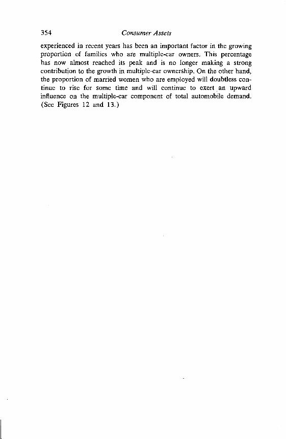
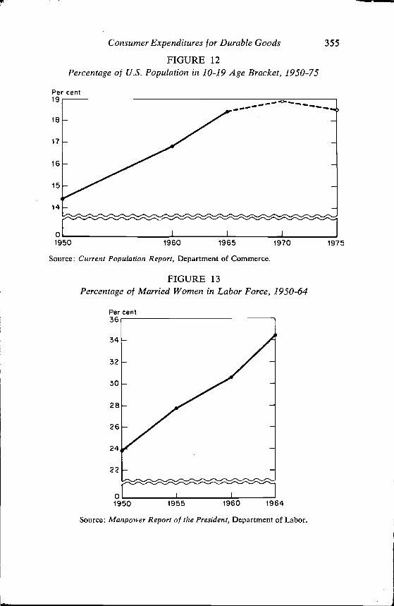
This has important consequences for the future of the automobilemarket. The sharp rise in the teen-age percentage of total population

Age of youngestthi Id

No. of weekswife worked

Variation explained: 18 per cent.Source: 1960-62 Survey of Consumer Finances. N-1059.

354 Consumer Assets

experienced in recent years has been an important factor in the growingproportion of families who are multiple-car owners. This percentagehas now almost reached its peak and is no longer making a strongcontribution to the growth in multiple-car ownership. On the other hand,the proportion of married women who are employed will doubtless con-tinue to rise for some time and will continue to exert an upwardinfluence on the multiple-car component of total automobile demand.(See Figures 12 and 13.)

Consumer Expenditures for Durable Goods

FIGURE 12Percentage of U.S. Population in 10-19 Age Bracket, 1950-75

Per cent19

16

17

16

15

14

01950 1960 1965 1970

Source: Current Population Report, Department of Commerce.

FIGURE 13Percentage of Married Women in Labor Force, 1950-64

Per cent36

34

32

30

28

26

24

22

355

1975

01950 1955 1960 1964

Source: Manpower Report of the President, Department of Labor