InstituteforInternationalEconomicPolicyWorkingPaperSeriesElliottSchoolofInternationalAffairsTheGeorgeWashingtonUniversity

UrbanizationwithandwithoutIndustrialization

IIEP-WP-2014-1

RémiJEDWABGeorgeWashingtonUniversity

DouglasGOLLINUniversityofOxford

DietrichVOLLRATHUniversityofHouston

October2013

InstituteforInternationalEconomicPolicy1957ESt.NW,Suite502Voice:(202)994-5320Fax:(202)994-5477Email:iiep@gwu.eduWeb:www.gwu.edu/~iiep

Urbanization with and without Industrialization∗

Douglas GOLLINa Rémi JEDWABb Dietrich VOLLRATHc

a Department of International Development, University of Oxfordb Department of Economics, George Washington University

c Department of Economics, University of Houston

This Version: October 1st, 2013

Abstract: Many theories link urbanization with industrialization; in partic-ular, with the production of tradable (and typically manufactured) goods.We document that the expected relationship between urbanization and thelevel of industrialization is not present in a sample of developing economies.The breakdown occurs due to a large sub-sample of resource exporters thathave urbanized without increasing output in either manufacturing or in-dustrial services such as finance. To account for these stylized facts, weconstruct a model of structural change that accommodates two differentpaths to high urbanization rates. The first involves the typical movementof labor from agriculture into industry, as in many models of structuralchange; this stylized pattern leads to what we term “production cities” thatproduce tradable goods. The second path is driven by the income effectof natural resource endowments: resource rents are spent on urban goodsand services, which gives rise to “consumption cities” that are made up pri-marily of workers in non-tradable services. We document empirically thatthere is such a distinction in the employment composition of cities betweendeveloping countries that rely on natural resource exports and those thatdo not. Our model and the supporting data suggest that urbanization isnot a homogenous event, and this has possible implications for long-rungrowth.

Keywords: Structural Change; Urbanization; IndustrializationJEL classification: L16; N10; N90; O18; O41; R10

∗Douglas Gollin, University of Oxford (e-mail: Douglas.Gollin@qeh.ox.ac.uk). Remi Jedwab, George Washington University(e-mail: jedwab@gwu.edu). Dietrich Vollrath, University of Houston (devollrath@uh.edu). We would like to thank NathanielBaum-Snow, Filipe Campante, Donald Davis, Gilles Duranton, Oded Galor, Edward Glaeser, Vernon Henderson, Berthold Her-rendorf, Fabian Lange, Margaret McMillan, Stelios Michalopoulos, Markus Poschke, Andres Rodriguez-Clare, Harris Selod, AdamStoreygard, Michael Waugh, David Weil, Adrian Wood, Anthony Yezer, Kei-Mu Yi and seminar audiences at Alicante, American,BREAD-World Bank Conference on Development in sub-Saharan Africa, Brown, Columbia, Durham, Eastern Economic Associa-tion, Georgetown (GCER), George Washington, McGill, NBER/EFJK Growth Group, NBER SI Urban Workshop, Oxford (CSAE),SFSU (PACDEV), World Bank, World Bank-GWU Conference on Urbanization and Poverty Reduction, Yonsei (SED Meeting) andYork. We gratefully acknowledge the support of the Institute for International Economic Policy and the Elliott School of Interna-tional Affairs (SOAR) at GWU.

1. INTRODUCTION

Many theories of development view urbanization and industrialization as essentially synonymous. In fact,the connection between the two is so strong that urbanization rates are often used as a proxy for incomeper capita (Acemoglu, Johnson & Robinson, 2002, 2005). Standard views reflect a stylized theory of thedevelopment process in which the process of structural transformation from agriculture into manufactur-ing and services involves a shift of labor out of rural areas and into urban ones. In typical closed-economymodels of this process, urbanization and the structural transformation are mechanically linked through acombination of a low income elasticity for food and the assumption that manufacturing and services arepredominantly or exclusively urban activities.

In this paper, however, we document that the expected relationship between urbanization and the levelof industrialization is absent in a sample of developing economies. Across countries today there is not aparticularly strong association between urbanization and industrialization, as proxied by the fraction ofGDP coming from manufacturing and services. Figure 1 plots this relationship for the year 2010 for 116countries, along with a quadratic fit. As can be seen, there are a number of countries that are highlyurbanized without having industrialized much. The data even point towards a negative relationship forcountries that are at particularly low levels of manufacturing and services in GDP.1

The breakdown occurs due to a large sub-sample of resource-exporting countries that have urbanized with-out increasing output in either manufacturing or industrial services. A clue to the source of urbanizationwithout industrialization can be found by noting that those countries with particularly high urbanizationrates but low shares of manufacturing and services in GDP are oil producers such as Brunei (BRN), Gabon(GAB), Libya (LBY), Kuwait (KWT), Qatar (QAT) and Venezuela (VEN). We define resource-exporters asthose in which natural resource exports make up more than 10% of GDP. They are represented by greysquares in figure 1.2 This disconnection can be seen more clearly in figure 2 in which we plot the relation-ship of urbanization and industrialization separately for resource-exporters and non-resource-exporters.Here we see that the non-exporters line up neatly with the expectations of standard models of structuralchange and growth, with urbanization tightly associated with the fraction of GDP coming from manufac-turing and services. In comparison, for resource-exporters, there is no tendency at all for urbanization ratesto be associated with industrialization. However, figure 3 shows that for these same resource-exporters,urbanization exhibits a strong positive correlation with their level of resource exports.

Growth economists are accustomed to ignoring major oil-producing countries in their analysis, as they donot fit into typical models of development. What figures 2 and 3 indicate, though, is that there are a hostof other countries that also deviate from the typical pattern of industrialization and urbanization seen infigure 1. One conclusion may be that all of the countries with natural resource exports over 10% of GDPshould be ignored when studying the “normal” process of development. However, that excludes nearly halfof our entire sample from consideration, many of which are African and Middle-Eastern countries.

In our view, the data suggest that urbanization can follow different patterns in different settings. Tobe sure, many countries conform with standard views of structural transformation. In these economies,urbanization is a by-product of either a “push” from agricultural productivity growth or a “pull” fromindustrial productivity growth. In these countries urbanization occurs with industrialization and generates“production cities,” with a mix of workers in tradable and non-tradable sectors. For a distinct subset ofcountries that rely on natural resource exports, however, urbanization has increased at an equally rapidpace, but urbanization has not been associated with growth in the manufacturing or service shares of GDP.In these countries, urbanization is driven by the income effect of natural resource endowments: resource

1Our definition of industrialization includes manufactured goods and industrial services such as finance and business services,as industrialized countries also have a comparative advantage in the production and export of these services (Jensen & Kletzer,2010). Tradable services now account for a large share of GDP for various countries, such as Hong Kong, South Korea or TheBahamas. This evolution of world output requires us to look beyond the manufacturing sector. As international sector data donot distinguish tradable and non-tradable services, we use services as an imperfect proxy for tradable services.

2Our definition of natural resource exports includes fuel, mining, cash crop and forestry exports. Cash crops include tropicalcrops such as cocoa, coffee and tea but excludes food staples such as maize, rice and wheat. A full list of the commodities includedin our calculation can be found in the Online Data Appendix.

2

rents are disproportionately spent on urban goods and services, which gives rise to “consumption cities”where the mix of workers is heavily skewed towards non-tradable services.

In the remainder of the paper, we further document a number of facts regarding urbanization and struc-tural change. In particular we show that the influence of natural resource exports on urbanization is robustto controlling for a variety of alternative explanations for urbanization. This holds in both cross-sectionaland panel regressions for our sample of 116 countries, and using different definitions of resource depen-dence. Following the existing literature (Sachs & Warner, 2001; Brückner, 2012; Henderson, Roberts &Storeygard, 2013), we use commodity price shocks and/or discoveries as instruments for natural resourceexports and show they have a causal effect on urbanization rates.

We then construct a model that can account for these facts. We adapt a standard model of structuralchange to explain how resource endowments can lead to urbanization as well as affect the sectoral com-position of the urban labor force. The driving force in the model is a standard Balassa-Samuelson effect inwhich income and substitution effects from resource exports lead to the growth of non-tradables produc-tion. We argue that this framework provides useful insights into why resource exporters have experiencedurbanization without industrialization. We also discuss how this path to urbanization may have implica-tions for the pace of long-run growth in these countries. It is not obvious that agglomeration externalitiesare found in non-tradable services to the extent that they are in manufacturing and tradable services, andtherefore urbanization without industrialization may lead to slower long-run growth.

In our model, the processes of urbanization and industrialization are driven by sources familiar from theliterature on structural change, but unlike that literature we will make a sharp distinction between theconcepts of urbanization and industrialization. An increase in income will shift demand away from goodsproduced in rural areas (food) and towards goods that tend to be produced in urban areas. These urbangoods will consist of industrial goods (manufactures and tradable services) as well as non-tradable goods(personal services and the like). An alternative source of urbanization is a change in relative productivities,which induces a substitution of labor towards the higher productivity sector. The effect of this on industri-alization and urbanization depends on precisely which sectors experience productivity changes.

This leads to several possible patterns of development within the model. A large endowment of naturalresources will lead to a strong income effect, shifting labor into urban areas, but as the relative produc-tivity of the industrial sector has not increased this will result in urbanization without industrialization.This particular pattern of urbanization involves what we call “consumption cities”, as their emergence isexplained by the consumption of a resource rent in the form of urban goods and services. These citiesconsist mainly of workers in non-tradable services, while the industrial goods are mainly imported fromabroad.3 A different path of development arises when industrial productivity increases. This also leads toan income effect that drives labor into urban areas, but the change in relative productivity implies that ur-banization is coincident with industrialization. This pattern involves what we term “production cities”, inthat the source of urbanization is industrialization itself. Production cities differ from consumption cities,in that their origin is different, which affects their sectoral composition, and hence their future prospectsfor growth.4

The model has several implications that we confirm hold in the data. First, our model suggests that the re-lationship of income per capita and urbanization should be similar regardless of the source of urbanization.We show that conditional on income per capita, urbanization rates are unrelated to the share of natural

3For example, The Economist (2012) writes: “Angola is now one of Africa’s economic successes - thanks almost entirely to oil.[...] Teams of gardeners are putting the finishing touches to manicured lawns, palm trees, tropical shrubs and paved walkways.Soon these will stretch the whole way along the Marginal, the seafront road that is being turned into a grand six-lane highwaysweeping around the horseshoe-shaped bay of Luanda, Angola’s buzzing capital. Modern offices, hotels and apartment blocksare sprouting up behind, replacing the pretty pink-and-white colonial buildings, drab crumbling flats and teeming shanty-towns.Across the bay, fancy yachts and speed boats crowd the shores of the Ilha, a once almost deserted strip of sand used mainly bypoor fishermen, on which smart restaurants and nightclubs for the new elite are now springing up. [...] Shiny shopping malls arefilled with everything the Angolan heart could desire, from gourmet food to the latest fashions and car models. Prices are wildlyinflated. Virtually everything, even basic building materials, still has to be imported.”

4Our theory says that any rent leads to an income effect that drives labor into urban areas. We focus on natural resourceexports because of the magnitude of their income effect. According to our estimates, they account for 10% of the developingworld’s GDP in 2010 (but one third in Africa and the Middle-East), against 1% for international aid and 1% for remittances.

3

resource exports in GDP or the share of manufacturing and services in GDP. Second, there is a distinctionin the pattern of trade depending on what drives urbanization. The model predicts that resource exporterswill import more food, industrial goods and services as a percent of GDP, conditional on their urbanizationrate and income per capita. We show that this holds in the data as well. Finally, because of the differentsources for urbanization, the composition of urban employment should differ between resource exportersand non-exporters. Using a novel data set on sector of employment for a set of countries we confirm thatcities in resource-exporting countries are “consumption cities”, with a larger fraction of workers in non-tradable services such as trade and transportation, personal and government services. Cities in countriesthat do not export significant resources are “production cities”, with more workers in industrial sectorssuch as manufacturing and tradable services.

Within the framework of our model, we consider the consequences of the different patterns of urbanizationon long-run outcomes. Many economists have argued that tradable manufacturing and service sectors arecapable of higher labor productivity growth than non-tradable services (Timmer & Vries, 2007; Duarte &Restuccia, 2010; Rodrik, 2011; Buera & Kaboski, 2012). In this case, the economic composition of urbanareas may matter for aggregate productivity growth. Natural resource exporters that urbanize through“consumption cities” will experience slower productivity growth than countries urbanizing according tothe standard model. By skewing the urban mix away from faster-growing sectors, in the long-run resource-exporters may end up urbanized but relatively less rich.

This paper is related to a large body of work on the role of sectoral labor productivity in driving structuralchange; i.e. the decline in agriculture, the rise and fall of manufacturing, and the rise of services (seeHerrendorf, Rogerson & Valentinyi 2011 for a survey of the literature). A first strand of the literature looksat the origins of structural change in developed countries. The “labor push” approach shows how a risein agricultural productivity (what we might think of as a Green Revolution) reduces the “food problem”and releases labor for the modern sector (Schultz, 1953; Matsuyama, 1992; Caselli & Coleman II, 2001;Gollin, Parente & Rogerson, 2002, 2007; Voigtländer & Voth, 2006; Nunn & Qian, 2011; Michaels, Rauch& Redding, 2012). The “labor pull” approach describes how a rise in non-agricultural productivity (anindustrial revolution) attracts underemployed labor from agriculture into the modern sector (Lewis, 1954;Harris & Todaro, 1970; Hansen & Prescott, 2002; Lucas, 2004; Alvarez-Cuadrado & Poschke, 2011). Wedocument that it is quite possible for an economy to urbanize without any change in agricultural andmanufacturing productivity, which are the only sources of structural change in standard models. Then, afew models actually consider an open economy and look at the interactions of trade and structural change(Matsuyama, 1992, 2009; Galor & Mountford, 2008; Yi & Zhang, 2011)

Our second contribution relates to the literature on urbanization and economic growth. First, a few studiesargue that some parts of the world have urbanized without it being explained by manufacturing growth(Hoselitz, 1955; Bairoch, 1988; Fay & Opal, 2000). This excessive urbanization is attributed to pull andpush factors feeding rural exodus, such as rural poverty (Barrios, Bertinelli & Strobl, 2006) or urban-biasedpolicies that led to overurbanization and urban primacy (Lipton, 1977; Bates, 1981; Ades & Glaeser, 1995;Davis & Henderson, 2003). Our paper shows that countries that did not experience manufacturing growthcan still urbanize with growth if they export natural resources. In line with Henderson, Roberts & Storey-gard (2013), we do not find that Africa is relatively urbanized for its level of economic development.Second, the literature suggests that agglomeration promotes growth, in both developed countries (Rosen-thal & Strange, 2004; Henderson, 2005; Glaeser & Gottlieb, 2009; Combes et al., 2012; Duranton & Puga,2013) and developing countries (Overman & Venables, 2005; Henderson, 2010; Felkner & Townsend,2011). Given that urbanization is a form of agglomeration, it has been argued that cities could promotegrowth in developing countries (Duranton, 2008; World Bank, 2009; Venables, 2010; McKinsey, 2011).5

However, Henderson (2003) does not find any effect of urbanization per se on economic growth. Howcan we reconcile the fact that there are strong agglomeration effects at the micro level (at the sector orcity level) but no growth effects at the macro level (at the country level)? It must be that some types of

5For instance, McKinsey (2011) writes (p.3-19): “Africa’s long-term growth also will increasingly reflect interrelated socialand demographic trends that are creating new engines of domestic growth. Chief among these are urbanization and the rise ofthe middle-class African consumer. [...] In many African countries, urbanization is boosting productivity (which rises as workersmove from agricultural work into urban jobs), demand and investment.”

4

urbanization are not as growth-enhancing as others and that cross-country regressions also capture theserather than just the best types.6 One possibility that our data raise is that the “consumption cities” thatarise in resource-exporters are less effective at generating productivity growth than the “production cities”seen in others.

Our “consumption cities” differ from the “consumer cities” of Glaeser, Kolko & Saiz (2001). Using U.S.data, they show that high amenity cities have grown faster than low amenity cities, and urban rents havegone up faster than urban wages. Our theory differs somewhat in that it is because income increases thatpeople spend more on urban goods and services, and hence that the country urbanizes. Weber (1922)also contrasts “consumption cities” and “‘production cities”: the former are primate cities that cater forthe needs of a political elite, while the latter address the needs of manufacturers and merchants. In hisview consumption cities emerge from rent redistribution rather than rent generation and they are thus notthat different from the “parasitic cities” of Hoselitz (1955) and the urban bias theory. Urbanization is notassociated with economic growth, in contrast to our theory. We argue that resource-exporters are moreurbanized simply because they are wealthier. If these countries also adopt urban-biased policies, this justaugments the initial effects of natural resource exports on urbanization.

Finally, this paper contributes to the literature on Dutch disease and the resource curse (Corden & Neary,1982; Matsuyama, 1992; Sachs & Warner, 2001; Harding & Venables, 2013). The mechanism that drivesthe rise of “consumption cities” in our model is the same as in a Dutch disease model - a boom in resourcerents shifts labor away from the tradable manufacturing sector and towards non-tradable services. Wedocument that this mechanism is able to explain a significant portion of the rapid urbanization seen inmuch of the developing world, a phenomenon overlooked by the Dutch disease literature to this point.Whether this constitutes a resource curse is not immediately clear. As we show, the high urbanization ratesin resource-exporters are driven by high incomes that are spent on urban goods and services, so in thatsense there is no curse. However, urbanizing through “consumption cities” may put a long-run drag ongrowth if non-tradable urban services do not experience productivity growth similar to the tradable sector,leading to a possible resource curse result.

The paper is organized as follows: Section 2 describes in greater detail the differential patterns of urbaniza-tion and industrialization. Section 3 presents our model, while section 4 compares its implications to thedata. Section 5 examines the long-run implications of these different patterns. Section 6 concludes.

2. PATTERNS OF URBANIZATION IN DEVELOPING COUNTRIES

Figures 1, 2 and 3 showed simple cross-sectional correlations between urbanization and industrializationfor a sample of countries. First, it is useful to consider patterns within specific regions of the world, asthey display the correlations more starkly. Second, we show that the correlations shown in the figures arerobust to controlling for other determinants of urbanization.

2.1 Regional Patterns of Urbanization

Latin America and the Caribbean (LAC) and the Middle-East and North Africa (MENA) are relativelymore urbanized than Africa and Asia, with urbanization rates about 80% and 60% in 2010 respectively.In both Africa and Asia, the urbanization rate was only 10-15% in 1950, which is characteristic of pre-industrial societies (Bairoch, 1988). It is now around 40%, as high as in developed countries after theIndustrial Revolution.7 Asia and the LAC region are examples of the standard story of urbanization with

6Overman & Venables (2005) explain that the extent of localization and urbanization economies varies substantially acrossindustries and across countries. Agglomeration effects seem to be larger in manufacturing and hi-tech services. Henderson (2003)shows that there is an optimal level of urban concentration, and significant deviations from this optimal level reduce growth.

7Appendix Figure 1 shows the urbanization rates for the four regions from 1950 to date. We do not include Western countriesin our analysis, as they were already highly urbanized in 1960. We also omit Eastern European and Central Asian countries dueto the lack of data before the end of the cold war in 1991. We then include the developed countries of Asia and the Middle-East,such as South Korea, Taiwan or Kuwait, as they were relatively poor and unurbanized in 1960. Our analysis is therefore focused

5

industrialization. The successful Asian and Latin American economies typically went through both a GreenRevolution and an industrial revolution, with urbanization following along as their economic activityshifted away from agricultural activities (Ranis, 1995; Stiglitz, 1996; Gollin, Parente & Rogerson, 2002,2007; Evenson & Gollin, 2003). A few exceptions are Brunei, Mongolia and Venezuela which were alsoheavily dependent on natural resource production post-1960. Some countries are both industrialized andresource-exporters, such as Chile, Indonesia, Malaysia, and Peru.

In contrast, Africa and the Middle East offer a perfect example of urbanization without industrialization.First, there has been little evidence of a Green Revolution in Sub-Saharan Africa. Its food yields haveremained low (Evenson & Gollin, 2003; Caselli, 2005; Restuccia, Yang & Zhu, 2008); in 2010, cerealyields were 2.8 times lower than in Asia, while yields were 2.1 times lower for starchy roots. Second,there has been no industrial revolution in Africa. Its manufacturing and service sectors are relatively smalland unproductive (McMillan & Rodrik, 2011; Badiane, 2011); in 2010, employment shares in industryand services were 5% and 29% for Africa, but 15% and 35% for Asia, and African labor productivity was1.9 and 2.3 times lower in industry and services, respectively (World Bank, 2013).8 Despite the lack of thestandard push out of agriculture or pull from industry, Africa has urbanized to the same level as Asia overthe last half-century. The relatively more urbanized countries export oil (e.g., Angola, Gabon and Nigeria),gold and/or diamonds (e.g., Botswana and South Africa), copper (e.g., Zambia) or cocoa (e.g., Ghana andIvory Coast). In the MENA countries, food yields are higher but arable land is scarcer. Most of them exportoil and are less industrialized than their Asian counterparts for the same income level. A few exceptionsare Jordan, Lebanon and Tunisia which are specialized in tradable services or manufacturing.9

Urbanization in resource-exporters is not driven by meaningful shifts of labor into urban areas to work inthe resource sector. Point-source resources are highly capital-intensive, and their production creates verylittle direct employment. For example, Angola’s urbanization rate was 15% before oil was discovered inthe 1960’s, but it was 60% in 2010 (an urban population of 11 million people). While oil now accountsfor over 50% of GDP it employs fewer than 10,000 nationals and a small number of expatriates. Botswanahas a similar urbanization rate to Angola, and while the diamond sector accounts for 36% of GDP, it onlyprovides employment for 13,000 people. Mining accounts for 1% of total urban employment on averagein our sample of resource-exporters. Cash crops are produced in rural areas and contribute to ruralemployment, rather than urban employment. Rather, urbanization in these areas appears to be driven bya natural resource revolution that provides a different origin for a “pull” into urban areas as the increasedpurchasing power made available from resources increases demand for urban goods.10

A related question is whether urbanization in Africa is different (Henderson, Roberts & Storeygard, 2013).Our claim is not that the effects of green, industrial or natural resource revolutions are different in Africathan in the rest of the world, but that Africa’s development path has thus far been tied closely to theproduction of primary products. We do not insist that this is an effect of resource endowments per se,nor do we take a geophysically deterministic view of development. Africa’s resource dependence is quitelikely endogenous, at some level. Resource dependence surely reflects historical patterns of institutionaldevelopment, in addition to geographic factors. In a proximate sense, though, we argue that resourcedependence accounts for a substantial part of the difference in urbanization patterns between Africa andAsia. We do not need to invoke African exceptionalism, either; the same forces shaping urbanization inAfrica also seem to explain patterns in the MENA region. Even within a single country, we can see evidencethat a green revolution, an industrial revolution and a natural resource revolution can all contribute to

on the developing world, which initially consisted of Africa, Asia (incl. the Middle-East) and Latin America.8There are exceptions to this broad characterization (McKinsey, 2011; Young, 2012). Growth has resumed in Africa, following

the economic reforms of the 1980s and the democratization wave of the 1990s. Some countries have diversified their economy,such as Mauritius and South Africa. However, most countries remain highly dependent upon resource exports.

9Appendix Figure 2 confirms that within Asia and Latin American and the Caribbean the expected pattern of urbanization andthe share of manufacturing and services in GDP holds up well. By comparison, Appendix Figure 3 shows that urbanization inAfrica and the Middle-East is positively associated with the importance of natural resources exports in GDP.

10Jedwab (2013) investigates the causal effect of the production of cocoa, a rural-based natural resource, on the growth ofcities in Ghana and Ivory Coast, using a natural experiment and district panel data spanning one century. In both countries, thecocoa farmers received about half of the resource rent and the government captured the rest. This distribution of the rent gaverise to a “dual” urban distribution consisting of small towns in the cocoa-producing areas and large government cities.

6

urbanization – as exemplified by countries such as Chile, Indonesia, Malaysia and South Africa.

2.2 Cross-Sectional and Panel Robustness Checks

Table 1 presents results of cross-sectional regressions using a sample of 116 countries (c) for the year 2010.The five columns use the urbanization rate in 2010 as the dependent variable (URBc,2010), regressed onthe average share of natural resource exports in GDP in 1960-2010 (NRX c,1960−2010) as well as the shareof manufacturing and services in GDP in 2010 (IN DUc,2010):11

URBc,2010 = α+ βNRX c,1960−2010+ γIN DUc,2010+ uc,2010 (1)

The regressions are all population weighted. Column (1) shows that across the entire sample, with noother control variables, both variables have a significant positive relationship with urbanization. Thepositive effect of manufacturing and services fits with the standard model of industrialization and urban-ization. However, the positive association of natural resource exports to urbanization is less obvious, giventhat natural resources employ very few urban workers directly. The positive effects of both persist whenwe include area fixed effects (Africa, Asia, LAC and MENA) in column (2).

There are several alternative theories for urbanization in developing countries that may make the resultsin columns (1) and (2) spurious. A few studies have argued that some parts of the world have urbanizedwithout it being fully explained by economic development. This excessive urbanization is attributed to pulland push factors feeding rural exodus. In the Harris-Todaro model, there will be rural-to-urban migrationas long as the (expected) urban wage is higher than the rural wage. First, land pressure and man-made ornatural disasters may result in a lower rural wage, with rural migrants flocking to the cities. We includethe following controls at the country level: rural density in 2010 (1000s of rural population per sq km ofarable area) and the annual population growth rate in 1960-2010 (%) to control for land pressure, and thenumber of droughts (per sq km) since 1960 and an indicator equal to one if the country has experienceda civil or interstate conflict since 1960 to control for disasters.12 Second, we include an indicator equalto one if the country’s average combined polity score since 1960 is strictly lower than -5 (the countryis then considered as autocratic according to Polity IV). We suppose that the urban bias was strongerin more autocratic regimes, as shown by Ades & Glaeser (1995). We also add the primacy rate (%) in2010, as an alternative measure of the urban bias. Third, if natural resource exporters systematicallyuse different methods for calculating urbanization rates, the correlations may simply reflect measurementerrors.13 We get around this issue by adding controls for the different possible definition of cities indifferent countries: four indicators for each type of urban definition used by the countries of our sample(administrative, threshold, threshold and administrative, and threshold plus condition) and the value of thepopulation threshold to define a locality as urban when this type of definition is used. Lastly, we alsocontrol for country area (sq km), country population (1000s), a dummy equal to one if the country isa small island (< 50,000 sq km) and an indicator equal to one if the country is landlocked, as larger,

11While the share of manufacturing and services in GDP in 2010 serves as a good proxy for the extent of industrializationin 1960-2010, the share of natural resource exports in GDP in 2010 does not measure well the historical dependence on nat-ural resource exports. First, many countries have recently started exporting oil such as Chad, Equatorial Guinea, Mauritania,Mozambique and Yemen. For these countries, the share of natural exports in GDP does not explain well the contemporaneousurbanization rate. Second, a few countries that were highly specialized in natural resource exports before have become moreindustrialized over time, such as Indonesia, Malaysia, Mauritius, Singapore and South Africa. Lastly, the contribution of naturalresource exports to GDP depends on international commodity prices, which are highly volatile in the short run. Using the averageshare of natural resource exports in 1960-2010 minimizes these concerns, as in Sachs & Warner (2001).

12Rapid population growth and land pressure could theoretically drive urban growth if the rural wage decreases. However,excess (urban) population growth could also decrease the urban wage. Ultimately, the urbanization rate only increases if urbangrowth is faster than rural growth, which is not obvious here. For example, we do not find any correlation between demographicgrowth and urbanization in the data. We nonetheless control for rural density and demographic growth in the regressions.

13Potts (2012) shows that the urbanization rate could be overestimated for a few countries for which the quality of the data ispoor. Our correlations are robust to dropping Nigeria and a few other countries that have been identified as problematical in theurban studies literature. Another issue is the fact that different countries use different urban definitions. This only affects ourestimates if the urbanization rate is systematically overestimated or underestimated in resource-exporters.

7

non-island and landlocked countries could be relatively less urbanized for various reasons.14

As can be seen in column (3), the inclusion of these controls does not alter the positive association ofnatural resource exports with urbanization rates. These correlations are very strong. A one standarddeviation in the share of natural resource exports in GDP is associated with a 0.48 standard deviationincrease in the urbanization rate. In comparison, a one standard deviation in the share of manufacturingand services in GDP is associated with a 0.39 standard deviation in the urbanization rate. Since half ofour sample consists of resource-exporters, industrialization and natural resource exports were possiblyequally important sources of urbanization in our sample. To address the possibility that the regressions incolumns (1) through (3) are still picking up an unobserved effect driving both urbanization and resourceexports, in column (4) we also control for initial conditions in 1960. Specifically, we include the level ofurbanization rate in 1960 (%) and the share of natural resource exports in GDP in 1960 (%). Thus column(4) is essentially like looking at a long-differenced relationship of the change in resource exports and thechange in urbanization. As can be seen, results are not altered much. Lastly, we can also include thirteenregion fixed effects (e.g., Western Africa, Central Africa, Eastern Africa and Southern Africa for Africa) tocompare neighboring countries. The point estimates remain high and significant (see column (5)).

We verify that these correlations are robust to (see Appendix Tables 2 and 3): (i) restricting the sampleto Africa and the MENA region or Asia and the LAC region only (the correlation of resource exports withurbanization is then not different in both groups), (ii) dropping China and India, due to their populationsize, or dropping population weights, (iii) controlling for the average share of manufacturing exports inGDP in 1960-2010 (%) as a proxy for industrialization, instead of using the share of manufacturing andservices in GDP in 2010 (%), (iv) using the share of resource exports in GDP in 2010 instead of the averageshare in 1960-2010, and (v) using the average log value of natural resource exports in 1960-2010 and thelog value of manufacturing and service GDP in 2010 instead of the GDP shares.15

When looking at the distinct correlations of fuel and mining exports and cash crop and forestry exportswith urbanization, we find that urbanization is not significantly associated with cash crop exports. We onlyfind a positive effect of cash crop and forestry exports for Africa countries, but this effect appears to bedriven by cocoa and forestry exports only, and not other crops. The correlations are then stronger for oilthan for other mineral resources, such as copper, diamonds and gold. Regarding cash crops, the correlationis only significant for cocoa, while no effect is found for other crops, such as coffee or sugar.16

We also test whether the results are robust to using a multivariate panel analysis for a sample of 112countries (c) and 6 years (t = [1960, 1970, 1980, 1990, 2000, 2010]). We investigate the correlationsbetween the share of natural resource exports in GDP at period t-1 (NRX c,t−1) and the urbanization rate atperiod t (URBc,t), while controlling for the share of manufacturing and services in GDP in 2010 interactedwith a time trend (IN DUc,2010× t) and adding country fixed effects (vc) and period fixed effects (wt). Asthe share of manufacturing and services in GDP is missing for many countries before 2010, we include theshare of manufacturing exports in GDP at period t-1 (M FGX c,t−1) to control for industrial booms. Sincewe examine the effects of variables at period t-1 on period t, we lose one round of data:

URBc,t = α′+ β ′NRX c,t−1+ γ

′ IN DUc,2010× t +κM FGX c,t−1+ vc +wt + u′c,t (2)

Standard errors are clustered at the country level. The unconditional results are shown in the column

14See Online Data Appendix for a description of the sources for all of these variables.15Wood (2003) uses total land area as a proxy for general natural resource wealth, citing the trouble of accurately measuring

resource wealth. We are using actual resource exports, as reported by the USGS (2013) and World Bank (2013), and are nottrying to impute values for natural resource stocks that may or may not exist. See Appendix for full details on how we constructthe resource export data series.

16These (non-)results on cash crops are in line with Jedwab (2013), who finds a positive causal effect of cocoa production onurban growth in Ghana and Ivory Coast, and Brückner (2012) and Henderson, Roberts & Storeygard (2013) who find a negativecausal effect of agricultural exports on urbanization in Africa when using agricultural price shocks as a source of identification.Positive price shocks may deter urbanization if workers are drawn into the agricultural sector, as in many two-sector models(Matsuyama, 1992; Henderson, Roberts & Storeygard, 2013). In our regressions, the correlation is negative for sugar. Countriesthat export cotton also appear to be relatively less urbanized. While the sugar industry contributed to the establishment of townsin the Caribbean during the colonial period, the development of the sugar beet industry in the 19th century probably reduced therents available in the sector. Likewise, the invention of synthetic fibers post-1930 reduced the rents available in the cotton sector.

8

(1) of Table 2. These results are robust to: (i) adding 20 continent-period fixed effects (see col. (2)),(ii) including the same controls as in Table 1 when they are time-varying, for example population growthbetween t-1 and t (see col. (3)), (iii) controlling for initial conditions (urbanization and natural resourceexports in 1960) interacted with a time trend (see col. (4)), and (iv) adding 65 region-period fixed effects(see col. (5)). The correlation between natural resource exports and urbanization is rather strong. A onestandard deviation in natural resource exports is associated with a 0.08-0.10 standard deviation in theurbanization rate. This correlation is fivefold lower than in the cross-sectional analysis. Cross-sectionaland panel estimates cannot be readily compared with each other. Panel regressions measure the short-termeffects of short-term variations in resource exports on urbanization, and permit the inclusion of countryfixed effects to control for time-invariant heterogeneity. Cross-sectional (and long-differenced) regressionsmeasure the long-term effects of long-term variations in natural resource exports. The cross-sectionalregressions could potentially capture the accumulation of short-term effects.

Are these cross-sectional and panel estimates causal? Natural resource exports could be endogenous tothe urbanization process.17 We could assume that resource production is exogenous (Harding & Venables,2013). The panel regressions appear to corroborate this hypothesis. In the column (5) of Table 2, weinclude 65 region-period fixed effects to ensure we compare neighboring countries over time. We alsoverify that urbanization has no effect on natural resource exports the next period, and that natural re-source exports have no contemporaneous effect on urbanization (see Appendix Table 4, columns 1 and2). Second, we expect stronger effects for point-source resources, as their international supply is relativelyinelastic and their production process is not labor-intensive, contrary to cash crops. We find strong effectsfor fuels and mining products, but no significant effects for cash crops, in both cross-sectional and panelregressions. In particular, we find stronger effects for oil than for other mineral resources, such as copper,diamonds or gold, or cash crops, such as cocoa. For instance, why a country would endogenously special-ize in oil rather than diamonds is not obvious, as it mostly depends on resource endowments, but we findsignificantly larger effects for the former (see Appendix Table 2).

As an alternative identification strategy we use resource discoveries or commodity price shocks as in-struments, as suggested by the literature (Sachs & Warner, 2001; Brückner, 2012; Henderson, Roberts &Storeygard, 2013). For each resource-exporter, we create a post-discovery indicator whose value is one ifthe country’s chief natural resource in 1960-2010 has already been “discovered” at period t-1. The effectof resource exports is then identified for these countries for which the discovery occurred post-1960. Forexample, figure 4 shows examples of countries that urbanized faster than their respective area (Africa orMENA) after a “discovery”: Angola (oil; 1968), Botswana (diamonds; 1971), Gabon (oil; 1963), Libya(oil; 1960) and Oman (oil; 1964). Another potential instrument is the price index of their main naturalresource. Zambia offers a perfect example of this identification strategy, as shown in figure 4. The slump incopper prices in 1975 clearly led to “counter-urbanization” in Zambia (Potts, 2005). Results are robust tousing discoveries or price shocks or both as instruments (see Appendix Table 4, columns 3–8). This workseven when restricting the sample to resource-exporters only (in that case, we simply compare the earlyand late discoverers). The IV estimates are higher than the OLS estimates, which thus provide a lowerbound of the true effects. However, the estimated effects could be local average treatment effects givingmore weight to those countries for which the instruments had a strong effect. Despite these concerns, theresults confirm the general patterns documented in the figures. Urbanization and industrialization shouldnot be seen as synonymous, as the presence of resource exports are significantly related to urbanizationrates.

3. A MODEL OF URBANIZATION AND INDUSTRIALIZATION

17It is not clear which way the bias would run. Urbanized countries could have fewer resources (e.g., land or labor) availablefor resource production. This would lead to a downward bias. Or, industrial countries may not export the natural resourcesthey produce if they use them as intermediary or consumption goods. For example, China and Mexico are among the top oilproducers. As these countries are also more urbanized, this leads to a downward bias. From the other side, investments indomestic transportation infrastructure both facilitate the exploitation of natural resources and promote urbanization, leading toupward bias. Poor institutions that foster an urban bias and restrict industry could also lead to high resource exports as well ashigh urbanization.

9

As seen in the data, the typical model of structural change is unlikely to be appropriate when describingindustrialization and urbanization in resource-exporters. Here we begin developing a model that incorpo-rates both resource-led urbanization as well as standard industrialization-led urbanization.

Our model is of a small economy open to international trade, with four specific-factor sectors in whichlabor can be employed. Tradables are produced in urban areas; this sector includes both manufacturingand tradable services such as finance. This is the sector associated with industrialization, and its outputcan be traded internationally at a world price. Non-tradables are also produced in urban areas. This sectorencompasses government and personal services, as well as construction, education and health, retail andwholesale trade and transportation.18 The output, unsurprisingly, cannot be traded internationally andso its relative price will be determined endogenously. Food is produced in rural areas and can be tradedinternationally. Resources are by assumption produced rurally and traded internationally at a given priceas well.19

There are two drivers of urbanization in the model: relative productivity and surplus income. An increasein tradable-sector productivity pulls labor in from other sectors, increasing both urbanization and indus-trialization at the same time. The increased productivity also increases income, and this will reinforce theeffect by increasing demand for urban goods in general. This generates what we term “production cities”,driven by the increased relative productivity of tradables.

There are alternative routes to urbanization, however. Increased productivity in the resource sector,whether through a discovery of new stocks of the resource or a sustained increase in the world price, alsodrives urbanization. The relative productivity effect suggests that labor is pulled out of the tradable sectorand into the resource sector. However, the surplus income generated from higher resource productivityincreases demand for non-tradables, and on net the urbanization rate rises. This type of urbanization,driven by the surplus income generated by resources, leads to what we term “consumption cities”. Thesecities are dominated by non-tradables if tradables are imported from abroad.20

To begin we develop the baseline model, and then provide extensions involving non-homotheticities indemand as well as urban-biased policies. In following sections we will discuss how the predictions of themodel match up against the data and explore its implications for long-run growth.

3.1 Individual Utility and Budgets

We assume that individuals have a log-linear utility function over three goods: food (c f ), tradable goods(cd), and non-tradable goods (cn),

U = β f ln c f + βd ln cd + βn ln cn (3)

where β f , βd , and βn are all between zero and one, and β f + βd + βn = 1. This utility function ishomothetic, unlike those typically used in models of structural change. We can demonstrate urbanizationwithout industrialization without using non-homotheticities in demand, and so in our baseline modelexclude them. After the main results, we show that non-homotheticities can be incorporated, and wefind that they exaggerate the effects. We note that resources do not enter the utility function directly forconsumers in our model economy; they will be produced only as a source of export earnings.

18Non-tradables also include manufactured goods that are produced locally and not traded internationally, for example“African” processed foods, clothing and furniture in Africa. These (home) goods differ from standardized manufactured goodssuch as vehicles, home appliances, computer hardware or equipment, that can be produced anywhere.

19As noted in footnote 2, it is self-evident that agricultural export crops such as cocoa, coffee and tea are produced in ruralareas; it is perhaps less obvious that minerals and other resources are produced in rural areas, but in the data it is difficult to findexamples of mining that takes place in heavily urbanized areas.

20This type of urbanization is a manifestation of the Balassa/Samuelson effect. Higher productivity in a tradable sector,resources, leads to an increase in the price of non-tradable goods. Here we focus on the associated shift of labor towardsthe non-tradable sector, which in this case implies an increase in urbanization as well.

10

Individuals earn an income m. The budget constraint for a consumer is given by:

p f c f + pd cd + pncn = m, (4)

where p j is the price of good j. Given the log-linear utility, the optimal choice for individuals is for theexpenditure share on good j to equal its weight in the utility function, β j ,

p jc j = β jm. (5)

The income of individuals is made up of four components: wages, resource rents, capital rents, andland rents. Wages are denoted by w. Assuming for now that productive assets are divided equally amongindividuals in the economy, the representative individual will earn a returnωr on R/L units of the resource,a return ωk on K/L units of capital, and a return ωx on X/L units of land. Income is therefore

m= w+ωrR

L+ωk

K

L+ωx

X

L. (6)

We will discuss below the implications of inequality in resource rent earnings, but given the log-linearutility the aggregate expenditure share on each good would still be β j .

21

3.2 Production, Factor Payments, and Trade

There are three domestic sectors producing each of the goods. Production is described by

Yd = Ad KαL1−αd (7)

Yf = A f XαL1−αf (8)

Yn = An Ln (9)

where A j ∈ ( f , d, n) is productivity in sector j, and L j is the labor used in that sector. Tradable goods areproduced using capital, K , while food goods are produced using land, X . Non-tradables use only labor.The value of α is assumed to be identical between the tradable and food sectors for simplicity.

We assume that the tradable and non-tradable sectors both operate exclusively in urban areas, while foodproduction is a rural activity. Therefore the urbanization rate, u, is the sum of the fraction of workers inthe tradable and non-tradable sectors:

u=Ld

L+

Ln

L. (10)

We do not explicitly model the increasing returns or agglomeration economies that determine productivityin urban sectors, or explain why tradables and non-tradables are located in urban areas. Rather, we focuson the static allocation of labor across the sectors, explaining urbanization through the broader processof structural change. Although not all tradable and non-tradable activity takes place in urban areas, ouremployment data for more than 40 countries in the 2000s shows that around 75% of manufacturing andservice activities are urban-based. Allowing for some fraction of tradable and non-tradable work to bedone in rural areas would not materially change our results.

We also do not explicitly model the accumulation of capital, nor do we endogenize the levels of produc-tivity in our baseline model. In the next section we consider the long-run consequences of urbanizationwithout industrialization, and at that point discuss how the model changes when capital accumulation orendogenous productivity is incorporated.

In addition to the three basic sectors, we introduce a resource sector that produces a good that can be sold

21Alternatively, one can think of the β j values as representing aggregate expenditure shares consistent with heterogenousindividuals with different preferences and wealth, or as representing aggregate expenditure shares consistent with a centralgovernment that earns the resource rents and makes decisions regarding how to spend those. Changing the β j shares will alterthe ultimate labor allocation in the economy, but not change our results regarding the influence of resources on those allocations.

11

internationally, but has no domestic market. It has a production function of

Yr = ArRγL1−γ

r , (11)

where Ar is total factor productivity, R is the size of the resource base, and Lr is the amount of labor usedin the sector. We purposely define the elasticity with respect to resources, γ , to differ from α. The valueof γ is a way of parametrically distinguishing between different types of resources. As γ goes to one, theoutput of the resource sector becomes like “manna from heaven,” and no labor effort is required to extractit. This would be the case for resources like oil or diamonds, where the labor force required for productionis very small relative to the population. As γ gets closer to α, labor is more important for the extraction ofthe resource, consistent with the production of cash crops.

3.3 Equilibrium

The economy is assumed to face world markets for the resource good, the tradable good, and food. Theirprices are exogenous to the economy, and given by p∗r , p∗d , and p∗f , respectively. The price of non-tradablegoods is pn and is determined endogenously. The sectors are all assumed to operate competitively, so thatthe stocks of resources, capital, and land all earn their marginal products,

ωr = γp∗rAr

Lr

R

1−γ(12)

ωk = αp∗dAd

Ld

K

1−α

ωx = αp∗f A f

L f

X

1−α

.

Labor is assumed to be mobile between sectors so that wages are equalized,

w = pnAn = (1−α)p∗dAd KαL−αd = (1−α)p∗f A f XαL−αf = (1− γ)p∗rArR

γL−γr . (13)

Labor mobility establishes several conditions regarding the relationships between the the fraction of laborengaged in the food, tradable, and resource sectors.

L f /L

Ld/L=

X

K

p∗f A f

p∗dAd

!1/α

(14)

(Ld/L)α

(Lr/L)γ=(1−α)p∗dAd(K/L)α

(1− γ)p∗rAr(R/L)γ

(L f /L)α

(Lr/L)γ=(1−α)p∗f A f (X/L)α

(1− γ)p∗rAr(R/L)γ.

While the possible difference between γ and α complicates the second two relationships, the conditionsare straightforward. Labor allocations between these three sectors depend on the relative productivity ofthe different sectors. If the world price or productivity of a sector rises, then its fraction of the labor forcerises relative to the other two. In particular, note that an increase in either p∗r , Ar , or R will increase therelative size of the resource labor force. To establish the size of these sectors relative to the non-tradablesector requires further conditions, as the price of non-tradables in endogenous. Given that non-tradablesare by definition only produced domestically, it must be that

βnmL = pnYn. (15)

12

The other three goods can be produced domestically and also imported or exported to the world market.Assuming balanced trade yields the following condition

(β f + βd)mL = p∗r Yr + p∗d Yd + p∗f Yf . (16)

This states simply that total expenditure on food and tradable goods must be equal to the total value ofproduction in the tradable sectors. To solve for the fraction of labor engaged in non-tradable production,divide (15) by (16), yielding

βn

β f + βd=

pnYn

p∗r Yr + p∗d Yd + p∗f Yf. (17)

Using the definitions of the production functions, and the fact that wages are equalized between sectors,this can be re-written as

βn

β f + βd=

Ln

Lr/(1− γ) + Ld/(1−α) + L f /(1−α). (18)

Given that L = Ln+ Ld + L f + Lr , this can be transformed to

Ln

L=

βn

1−α(βd + β f )

1+γ−α1− γ

Lr

L

, (19)

which gives the level of Ln as a positive function of the level of Lr . From this expression one can begin tosee how resources will influence urbanization and structural change. Anything that raises the fraction oflabor engaged in resource production will increase non-tradable employment. If there are no resources inthe economy, then Lr/L = 0, and the model reduces to the typical result that the labor share depends onthe expenditure share for non-tradables.22

3.4 Urbanization without Industrialization

Consistent with the empirical regularities documented earlier, in our model an increased stock of naturalresources (or an increased price for those resources on the world market) will generate urbanizationwithout industrialization. When resource labor productivity goes up (whether through p∗r , Ar , or R), thenLr/L will rise relative to both L f /L and Ld/L, as seen in (14). This is a classic Rybczynski effect. Thefall in Ld/L implies a fall in industrialization in the economy. The non-tradable sector responds differentlyprecisely because it is non-tradable. The increased productivity in resources represents a real increasein earnings, and so individuals demand more of each of the consumed goods. The only way to providemore non-tradable goods is to increase the fraction of workers in that sector, which is what equation (19)captures. With labor flowing into non-tradables, it must be that the price pn is rising as well to ensure thatthe wage remains identical to the alternatives. When resource productivity increases the economy canincrease its consumption of food and tradables through imports, and so those sectors can shrink relativeto resources and non-tradables. Under plausible conditions that we document below, the increase in Ln/Lwill outweight the fall in Ld/L, and overall the urbanization rate will increase following an increase inresource productivity. Hence we have urbanization without industrialization, and as this urbanization isdriven by increased demand for non-tradable goods, we have “consumption cities”. This is all presentedmore formally in the following proposition and corollary.

Proposition 1. Given the labor market equilibrium conditions given in (14) and (19), and an increase in theprice of the resource (p∗r), the productivity of the resource sector (Ar), or the size of the resource base (R), itwill be true that:

• (A) Lr/L increases

22The leading fraction βn/(1−α(βd + β f )) reflects the expenditure share on non-tradables, βn, but is adjusted by the term inthe denominator because the labor elasticity of production differs between sectors. As there are not diminishing returns to laborin non-tradables, the economy will tend to put more labor in that sector in equilibrium.

13

• (B) Ln/L increases

• (C) L f /L and Ld/L decrease

• (D) The ratio of non-tradable to tradable employment - Ln/Ld - will increase

• (E) The price of non-tradable goods, pn, increases

Proof. (A) follows from the labor market conditions in (14), the relationship of non-tradable to resourcelabor in (19), and the adding up constraint L f + Ld + Lr + Ln = 1. Using (14) and (19), one can write theadding up constraint in terms of only Lr . This is an implicit function determining Lr . Using the implicitfunction theorem, the derivative ∂ Lr/∂ Ar > 0. The partial derivative with respect to p∗r and R followsfrom the same function. (B) follows directly from (19) and part (A). (C) follows by noting that if bothLn/L and Lr/L increase, then the sum L f /L+ Ld/L must decrease. From (14) the ratio of L f /Ld does notchange when Ar , p∗r , or R increases, so both L f /L and Ld/L must actually fall. (D) follows from parts (B)and (C). (E) can be seen from the equalization of wages between non-tradables and tradables. Given thatLd/L falls, it must be that the wage paid in the tradables sector rises. The wage in the non-tradables sectoris pnAn, so the only way for this wage to rise to keep the labor market in equilibrium is for pn to rise.

The proposition establishes the shift in labor allocations that take place with higher productivity in theresource sector (whether through an increase in the endowment, actual productivity, or the world price).This change in labor allocations does not involve industrialization: labor is actively moving out of tradablegood production. However, the overall effect on the urbanization rate is ambiguous, given that Ln/L isrising. This proposition contains elements of the typical “Dutch Disease” description of resource-exporters.In those models, the focus is the relative productivity effect, and the transfer of labor out of tradables andinto resources. However, the Dutch Disease models generally ignore the effect of the increased incomefrom resources on the allocation of labor into alternative sectors. These models do not typically focus onurbanization, and as such they do not emphasize the implications for urbanization of increases in resourceproductivity. The next corollary establishes that urbanization in the economy increases with resourceproductivity as long as the initial fraction of labor in tradables is sufficiently small.

Corollary 1. If the following condition holds:

Ld

L f<γ−α1− γ

βn

1−α(βd + β f )(20)

then an increase in p∗r , Ar , or R will result in a net increase in the urbanization rate u.

Proof. See appendix

When resource productivity rises, labor is pulled out of both the food and tradable sectors. As the ratioof Ld/L f must remain constant, the absolute change in Ld depends on how much tradable labor there isto begin with. The condition in the corollary states that so long as Ld is sufficiently small compared to L fthen the loss of labor in tradables will not offset the rise of labor in non-tradables, and urbanization willincrease. Practically, for countries that have little to no tradable sector to begin with, i.e. countries whoseurbanization rate is close to 0, increasing resources will increase urbanization. On the contrary, DutchDisease models are applicable for countries who are already industrialized and urbanized.

Note that the degree of urbanization following an increase in resource production depends on the size ofγ relative to α. See the expression for Ln/L in equation (19) to see this explicitly. For economies withresources characterized by a large γ, such as oil, a relatively small change in the labor share in resourceswill produce a large shift towards non-tradable work. The reason is that there are two effects at workwhen resource productivity increases. First, the change in relative productivity induces labor to move intoresource production. Second, the increased income due to the productivity improvement raises demandfor non-tradable goods, which pulls labor out of the other sectors. When γ approaches α, the first effectoffsets the second, and there is no net change in labor in non-tradables. When γ approaches one, then

14

a very small shift of labor into resources is sufficient to equalize wages across sectors, and so on net thesecond effect dominates the first.

Last, it is worth considering an economy without any resources as a comparison. If we set R = 0, thenthe resource sector is shut down completely, and Lr/L = 0. From (19) the fraction of labor in the non-tradable sector is given by Ln/L = βn/(1 − α(βd + β f )), which is fixed by the expenditure shares. Forthe non-resource economy, the only way that urbanization proceeds is for the ratio of tradable labor tofood labor, Ld/L f , to increase. This occurs, from (14), only if Ad increases relative to A f .23 Withoutresources, the process of urbanization is thus entirely coincident with the process of industrialization.Urbanization driven entirely by changes in relative productivity leads to what we call “production cities”.Within countries that do not have significant natural resource exports we see just such a relationship.

3.5 Subsistence Constraints

Incorporating a subsistence constraint for food consumption, and thus introducing a non-homotheticityof the kind common in models of structural transformation, is straightforward. Let c f be the subsistencerequirement for individual food consumption, and utility be given by:

U = β f ln(c f − c f ) + βd ln cd + βn ln cn. (21)

This leads to an income elasticity of demand for food that is less than one. The budget constraint forindividuals can now be written in the following manner:

p f (c f − c f ) + pd cd + pncn = m− p f c f , (22)

where the term on the right is now surplus income. The preferences are such that individuals will consumea fraction β j of their surplus income on good j, as before. The difference for food is that individualsconsume fraction β f of their surplus income on surplus food, (c f − c f ). So total expenditures on food areβ f (m− p f c f ) + p f c f .

Combining these preferences with the production structure outlined above, we have similar conditionsregarding total expenditures and total production of the non-traded good,

βn(m− p f c f )L = pnYn. (23)

Again, the other three goods are internationally tradable, and balanced trade dictates the following rela-tionship

(β f + βd)(m− p f c f )L+ p f c f L = p∗r Yr + p∗d Yd + p∗f Yf . (24)

Solving these together as before yields a relationship between Ln/L and Lr/L,

Ln

L=

βn

1−α(βd + β f )

1+γ−α1− γ

Lr

L−

p f c f

pnAn

. (25)

The relationship is similar to what we found without the subsistence constraint. However, there is nowan additional term - the fraction p f c f /pnAn - that will act to determine the size of the non-tradablesector. This additional term will exaggerate the effect of resources on the fraction of labor in the non-tradable sector. Mechanically, when resource productivity rises the fraction Lr/L will go up, as alreadyestablished. The Balassa-Samuelson effect dictates that pn will rise as well. As p f is fixed, that meansthat the additional term in (25) falls in absolute value. Given that it enters the equation negatively, thisresults in an additional increase in Ln/L. More intuitively, when resource productivity rises individuals inthe economy have become richer. The subsistence constraint ensures that the income elasticity for food isless than one, and hence the additional income is spent disproportionately on non-food goods. Note thatthis effect will arise no matter the source of the income gain. Increases in tradable or food productivity

23However, with non-homothetic preferences, any increase in food productivity A f should also drive urbanization.

15

will increase the fraction of labor in non-tradables, as in typical models of structural change.

3.6 Inequality in Distribution and Urban Bias

In the baseline model we assumed log-linear preferences, and hence all individuals spend the same fractionof their income on each good. Practically, this means that the distribution of resource rents (or of incomein general) does not influence the allocation of labor across sectors.

However, it is a near certainty that resource rents are concentrated on a small number of individuals, whosepreferences differ from the average – either because of non-homotheticity or because of pure differencesin preferences. For example, rich people may receive disproportionate shares of resource rents and mayprefer to spend the money on housing services and personal services. Alternatively, although we do notattempt to model a government sector formally, we could imagine that governments receive all the rentsfrom certain resources (e.g., minerals) and spend these rents on the provision of non-tradable publicservices in urban areas. (This would be consistent with a political economy of “urban bias,” for example.)We could represent this urban-biased government, in a highly reduced form, as a single rent-earning agentwho chooses to consume her income in the form of non-tradable services.

To allow for this in the model, consider the following modification. Let there be a class of individuals thatearn wages, capital returns, and land returns as before. These individuals have preferences over the threegoods as in the baseline model, with weights β f , βd , and βn.

In addition, there is some group for that earns wages, capital returns, and land returns as before. However,this group also earns all of the resource rents in the economy. This group has a set of preferences that islog-linear, but with weights θ f , θd , and θn. The idea is that these individuals will, due to their resourcerents, prefer more urban goods. Additionally, they are likely to disproportionately spend their income onnon-tradable goods such as government or personal services. So presumably θn > βn.24

Let the group of resource owners be a fraction λ of the total population, and hence the non-resourceowners are a fraction 1−λ. With these two groups, the condition relating expenditures and production inthe non-tradable sector is

βn

wL+ωkK +ωx X

+ θnωrR= pnYn, (26)

where βn = βn(1− λ) + θnλ is simply the weighted average of the two expenditure shares. In a similarmanner, the condition for the food and tradable sectors, given balanced trade, is

(β f + βd)

wL +ωkK +ωx X

+ (θ f + θd)ωrR= p∗r Yr + p∗d Yd + p∗f Yf . (27)

Here, β f and βd are defined similarly to βn, as the weighted average of the expenditure shares of thetwo different groups. These conditions can be solved together similar to before, yielding the followingrelationship between non-tradable labor and resource labor,

Ln

L=

βn

1−α(βd + β f )

1+γ−α1− γ

Lr

L

+1−α

1−α(βd + β f )

γ

1− γ(θn− βn)

Lr

L. (28)

Again, the relationship present here is similar to the baseline model, but the expenditure shares are theβ j terms, reflecting the weighted average of expenditure shares of the two types of people. This simplyreflects the heterogeneity in preferences. The second term on the right hand side of (28) reflects the factthat one group of people has a disproportionate share of the resource income. The key part of this newterm is (θn − βn), which is the difference in the expenditure share of resource-owners and the weightedaverage across all individuals. Assuming that resource-owners prefer non-tradable goods more than theaverage, then anything that raises Lr/L will have an even stronger effect on Ln/L than in our baselinemodel. Simply, the only reason Lr/L will rise is if the productivity of the resource sector increases, and this

24This is also a crude method of capturing non-homotheticities, where the resource-owners spend less of their income on staplegoods like food, and more on luxuries such as personal services.

16

implies that the rents accruing to resource-owners are increasing as well. As they demand non-tradablesmore than the average person, this skews demand towards non-tradable goods and Ln/L rises.25

The implication of (28) is that the increase in urbanization following a positive shock to resource pro-ductivity depends on the degree of inequality as well as the difference in preferences across groups. Thedifference θn− βn is maximized when λ goes to zero, or there is a vanishingly small group of people whoearn the resource rents. Hence, inequality in the earning of resource rents, along with an “urban bias” inthe preferences of the resource rent owners, will exaggerate the urbanization effects of resources. How-ever, note that an urban bias in the preferences of resource rent owners is not necessary for resources todrive urbanization, as the baseline model shows.

4. IMPLICATIONS FOR URBANIZATION AND INDUSTRIALIZATION

The static model we have laid out shows how urbanization can occur without industrialization in resource-exporters. The model has several other implications that distinguish these resource-exporters from thosefollowing the “typical” path of urbanization with industrialization. Here we establish that these implica-tions are consistent with the observed data.

4.1 Urbanization, Income and Trade

Figure 5 displays several comparative static results from the model. The statics are for variation in the sizeof the resource endowment. Panel (A) shows what we have already established above, that urbanizationrates rise with the share of resource exports relative to GDP. As seen in the introduction and section2, there is a significant correlation between the two in the data. That correlation is driven entirely bymineral resources as opposed to cash crops. The clear relationship demonstrated in figure 5 is due in partto a high value of γ, which would be consistent with mineral resources that do not require an intenseamount of labor. Cash crops would have a different, less pronounced, relationship between resources andurbanization, due to a smaller value of γ. In combination, this can explain the lack of any significantrelationship between cash crops and urbanization in the data.26

Panel (B) shows that, ceteris paribus, a greater share of resource exports in GDP is also associated withhigher income per capita. Increasing the endowment of resources increases the income of a country, andthis increased income is one of the driving forces of urbanization, as explained above. Panels (A) and(B), taken together, indicate that urbanization and income per capita are positively correlated even forcountries that urbanize due to increased resource endowments. The data confirm that the cross-sectionalrelationship between resources and urbanization operates through income effects. In table 3 we displayregressions confirming this. In column (1) we show that both resource-exporters and industrial countriesare relatively wealthier than other countries. Column (2) replicates our earlier result that natural resourceexports are positively related to urbanization (see column (3) of Table 1). In column (3) we control forGDP per capita, and as can be seen the independent effect of resources is both insignificant and falls toalmost zero.27 The implication of this result is that urbanization is driven by income per capita; whetherthis income per capita comes from industrialization or resources is not relevant. Note that in column (2),the positive effect of manufacturing and services on urbanization is also statistically zero. Column (2)

25Note that this set-up nests our baseline model. If there is no inequality, or λ = 1, then θn will be identical to βn, and thesecond term in (28) goes to zero. Alternatively, if both groups have identical preferences, then regardless of the distribution ofresource rents θn will be equal to βn.

26This can also explain why significant cash crop exporters of the past, such as the cotton, sugar, and tobacco plantations ofthe Americas, or the western African traders of salt, gold, and ivory, did not urbanize to the extent we see in modern times. Evenwith high prices for those goods at the time, the low value of γ would have limited the impact on urbanization. As the number ofproducers of those cash crops expanded over time the relative price dropped, further limiting the urbanization that is associatedwith those goods. The consumption cities of modern times rely on mineral exports, and differ from the consumption cities of thepast in that the global demand for their products is high while their production costs are relatively low (a high p∗r for a low γ).

27As explained in footnote 11, there are a number of reasons why we use the average share of natural resource exports in GDPin 1960-2010 instead of the same share for the year 2010 only. Likewise, we must use average GDP per capita in 1960-2010, asGDP per capita in 2010 imperfectly captures the effect of natural resource exports in 1960-2010 on urbanization in 2010.

17

shows that resource-exporters do not have a fundamentally different relationship between urbanizationand income per capita than typical developing countries.

If urbanization is just a story of income per capita growth, then why have we focused so much on therole of resources? The answer is that the source of the income per capita growth has implications forthe type of urbanization that occurs. As discussed earlier, resource-dependent economies develop through“consumption cities”, where urbanization rises due to the surplus income generated. One aspect of thesecities is that they necessitate increasing imports of both food and industrial goods and services, as thosesectors are shrinking (or not developing) due to the resource sector’s comparative advantage. This canbe seen in our model in figure 5 panel (C), which plots food imports and tradable imports as a share ofGDP against resource productivity. Imports of both are increasing as fractions of GDP as resource exportsbecome a larger fraction of GDP. We can see this increased import activity in the data as well. Table 3 showsin column (4)-(8) the results of regressions of various types of imports as a share of GDP on our measuresof economic structure, as well as income per capita and the urbanization rate itself. As can be seen incolumn (4), the greater the share of resource exports in GDP, the higher food imports tend to be. Theeffect of a higher manufacturing and services share is smaller in estimated value. An F-test for the equalityof the coefficients on resources and manufacturing/services (shown in the second panel) shows strongevidence that the coefficients are statistically different. This result holds if we consider staple food importsinstead (see column (5)). In column (6) the dependent variable is manufacturing imports as a share ofGDP. Resource-exporters import more manufactured goods than industrial countries, but not significantlyso (the F-test is only significant at 14%). Industrial countries may also import more manufactured goodsfrom other industrial countries to diversify their consumption of such goods. Lastly, resource-exportersimport significantly more (tradable) services than industrial countries, for the same economic conditions(see column (7)).

4.2 Sectoral Composition of Cities

Another aspect of urbanization without industrialization is the workforce composition of consumptioncities. When resource productivity rises, this shifts labor out of the tradable sector but increases demandfor urban non-tradables. Hence consumption cities are composed mainly of non-tradable workers. Thepatterns of employment predicted by the model can be seen clearly in panel (D) of figure 5. The solid lineshows the fraction of workers in the food sector, which steadily declines as resource productivity rises -this is the counterpart of the increasing imports of food seen in panel (C). There has been no increase infood productivity, so food demand must be met by increased imports as workers leave rural areas. Thoseworkers are finding their way, almost exclusively, into the non-tradable sector. There is some small increasein the share working in the resource sector. The exact size of the shift into the resource sector depends onthe size of the γ parameter, so in different situations the shift into resources may be larger or smaller thanwhat we have depicted here. However, what is unambiguous is that the composition of urban workersis becoming almost entirely skewed towards non-tradables. The gray dashed line at the bottom of panel(D) is the share engaged in tradable production. Taken together with the rise in non-tradable workers, itfollows mechanically that urban areas are growing larger but not industrializing.

First, we have data that corroborates this dominance of non-tradable workers in the cities of resource-exporters. As described in the Online Data Appendix, we use IPUMS census, labor force survey andhousehold survey data to recreate the sectoral composition of urban areas for as many countries as possiblein 2000-2010. For each country, we know the urban employment shares of 11 sectors.28 We focus on urbantradables, i.e. “manufacturing” (Manuf.), and “finance, insurance, real estate and business services” (FIRE)as an imperfect proxy for tradable services. Figure 6 shows the relationship between the share of urbantradables in total urban employment (%) and the contribution of natural resource exports to GDP (%) for87 countries in 2000-2010. These countries represent 95% of the whole sample’s population. As expected,

28We use data for the most recent year. When no data could be found for the period 2000-2010, we use data for the 1990s.Similarly to McMillan & Rodrik (2011), the 11 sectors are: “agriculture”, “mining”, “public utilities”, “manufacturing”, “construc-tion”, “wholesale and retail trade, hotels and restaurants”, “transportation, storage and communications”, “finance, insurance,real estate and business services”, “government services”, “education and health” and “personal and other services”.

18

we find a strong negative relationship between urban tradables employment and natural resource exports.In column (1) of Table 4 we verify that this result holds when we include area fixed effects, the samecontrols as in Table 1, as well as GDP per capita and the urbanization rate.29 The urban employment shareof urban tradables is significantly lower in resource-exporters than in industrial countries for the sameeconomic conditions (see the F-test in the second panel).

The highly industrial countries in our sample (e.g, those countries whose share of manufacturing andservices in GDP is above 70%) and the heavy resource-exporters (e.g., those countries whose share ofnatural resource exports in GDP is above 20%) are all highly urbanized, with urbanization rates around60% on average for both groups. In the highly industrial countries, urban tradables account for 30% ofthe urban workforce, against 10% in the heavy resource-exporters. When examining other sectors, we findthat the gap (20 percentage points) is mostly explained by the shares of “commerce and personal services”and “government services” being relatively higher in the resource-exporters (+ 16 and 2 percentage pointsrespectively).30 In column (2) and (3) of Table 4 we verify that the labor shares of these sectors aresignificantly higher in resource-exporters than in industrial countries for the same economic conditions.The F-tests confirm that this is indeed the case. The result for the commerce sector is in line with the model,as resource-exporters import a larger share of their food and tradables consumption. Their cities serve asdistribution stations for imported goods that are then dispatched to the rest of the country. Additionally,resource rents create shops and restaurants for the wealthy, but also for those who cater for the needs ofthe wealthy and so on (see footnote 3 on Angola). The results for government services are also in line withthe model: the government may receive resource rents that it could spend on the provision of non-tradablepublic services (or the hiring of additional government employees).

Second, the fact that countries use different urban definitions could affect the urban employment share ofurban tradables. A restrictive urban definition would mechanically exclude small agriculturally orientedtowns, while a narrow urban definition would only select large cities with a strong manufacturing sector.We verify that the results of columns (1)-(3) hold when we use the same type of data for the largest cityonly of 84 countries. Column (4) shows that the urban employment share of tradables is significantlylower in resource-exporters than in industrial countries, when using this alternative sample.

We also verify that these results on the compositional mix of cities are robust to using the urban laborshare of skilled workers as an alternative measure of urban tradables. We use IPUMS census, labor forcesurvey and household survey data to recreate the occupational composition of urban areas for more orless the same countries as before.31 We focus on skilled workers, i.e. “professionals” and “techniciansand associate professionals”. In column (5) we regress the share of skilled workers in all urban areason the same variables as before. While the occupational effects are less precisely estimated than thesectoral effects, cities in resource-exporters appear to have relatively fewer skilled workers than cities inindustrial countries for the same income level (see the F-test). Interestingly, we also find that cities inresource-exporters have relatively more “service workers and shop and market salesmen” and “clerks”(not shown but available upon request). These two results seem to be in line with the results of column(2) and (3) respectively, the fact that these cities have larger commerce, personal service, and governmentsectors.

Third, an alternative explanation is that the productivity level of non-tradables is systematically higher inresource-exporters, and so the “consumption cities” we observe are not directly the result of resources, butjust reflet relative productivity differences. Due to poor comparable data on urban wages in the developingworld, we cannot directly address this question.32 As an alternative, for 111 countries of our sample, we

29For example, Kuwait and Japan have similar per capita incomes and urbanization rates, but Kuwaiti cities have a loweremployment share of tradables (11% vs. 33%). Other pairs of countries for which we corroborate this hypothesis are: SaudiArabia vs. South Korea and Taiwan; Gabon and Libya vs. Mexico, Chile and Malaysia ; and Angola vs. China and The Philippines.

30The “commerce and personal services” sector consists of “wholesale and retail trade, hotels and restaurants”, “transportation,storage and communications” and “personal and other services”. We lump them together to capture the whole commerce sector.

31We use data for the most recent year. When no data could be found for the period 2000-2010, we use data for the 1990s.The 9 occupations are (armed forces are excluded from the analysis): “legislators, senior officials and managers”, “professionals”,“technicians and associate professionals”, “clerks”, “service workers and shop and market sales”, “skilled agricultural and fisheryworkers”, “crafts and related trades workers”, “plant and machine operators and assemblers” and “elementary occupations”.

32Gollin, Lagakos & Waugh (2011) use household survey data to show that the value added per worker in developing countries

19

calculated manufacturing and service productivity for the most recent year available in 2000-2010. Incolumn (6) the dependent variable is manufacturing productivity. We do not find any significant differencebetween resource-exporters and industrial countries (see the F-test), although the point estimate is higherin the latter countries. In column (7) the dependent variable is service productivity. The service sectorappears to be relatively less productive in resource-exporters than in industrial countries for the sameeconomic conditions. The results of columns (6) and (7) would suggest that cities in resource-exporterswould have a tendency towards more manufacturing employment if relative productivity were all thatmattered. Yet we see resource-exporters with a higher share of workers in services, and in particularin low productivity non-tradable services. McMillan & Rodrik (2011) shows that labor productivity isthree times higher in the FIRE sector than in “wholesale and retail trade, hotels and restaurants” and“community, social, personal and government services” for the world in 2005 (see their Table 2). Theseresults should be taken with some caution. Obviously, it is partly because tradable sector productivity islow in resource-exporters that they have a comparative advantage in resource exports. These results areuseful as another robustness test of the results based on actual employment data.

Finally, we did not take any stand on the distribution of resource rents, and so the model does not haveany explicit predictions regarding either the type of non-tradable employment in urban areas, or on whichcities (primate or otherwise) will be particularly affected by resource rents. However, we are able to offerseveral additional pieces of data regarding the relationship between resource rents and the compositionof urban employment. In table 4, columns (2) and (3) indicate that the employment effect of naturalresources acts primarily through commerce and personal services, and only marginally through increasedgovernment employment.

Similarly, we see no tendency towards urban primacy being driven by natural resource exports. We re-gressed the population share of the largest city (or alternatively the top 5 cities) in 2010 on natural resoureexports, while also controlling for manufacturing and services share of GDP and the urbanization rate. Theresults (shown in Appendix Table 5) show that there is no significant effect of natural resource exports onprimacy once we include area fixed effects. Resource exporters do not appear to concentrate the urbanpopulation more highly than in other countries. Neither this result nor the prior one give any informationon who precisely earns the resource rents in an economy, but they do indicate that the main effect of thoserents is to increase spending on commerce and personal services across all the urban areas of the economy.There is no evidence of a systematic tendency for a increased concentration of government employees inthe primate city.

5. URBANIZATION AND LONG-RUN GROWTH

It is commonly assumed that urban agglomerations are centers of productivity growth, both in developedand developing countries. Greater urbanization should therefore lead to faster growth. This expectedrelationship has been embedded into growth models to describe the divergence in output per capita acrosscountries. However, growth is not strongly affected by urbanization per se in cross-country regressions.33

The question then is, how we can reconcile the micro-evidence, which indicates large agglomerationeconomies, and the macro-evidence, which does not show any growth effect of urbanization?

Most of the literature presumes that urban areas are essentially identical across countries in their economicstructure. But perhaps agglomeration effects on productivity are more pronounced in manufacturingthan in non-tradable services. The underlying assumption of the agglomeration literature is that citiesare “production cities”, with a mix of tradable good production (often manufacturing) and non-tradableproduction (often services). However, as we have documented, for a large group of countries urban

is still relatively higher in the non-agriculture sector than in agriculture. But they do not directly investigate whether the urbanwage is relatively higher in some countries than in others. Data from McMillan & Rodrik (2011) indicate that mining produc-tivity is not necessarily lower in developing countries than in developed countries. But their data set does not tell us whethermanufacturing and service productivity is lower in resource-exporters than in industrial countries with a similar income level.

33We also test this non-result by regressing economic growth in 2000-2010 (1960-2010) on urbanization in 2000 (1960),while simultaneously controlling for initial per capita GDP in 2000 (1960) and adding area (or region) fixed effects and the samecontrols as before. We find that the coefficient of the urbanization rate variable is nil.

20

areas are skewed towards non-tradable production in “consumption cities”. In this case, cities are notall the same. Agglomeration effects might be present for certain sectors, but a regression including both“consumption” and “prouction” cities would give inconclusive results on urbanization and growth.

5.1 Mechanisms

There are several lines of research that suggest production cities will have greater long-run productivitygrowth than consumption cities:

• Manufacturing convergence: There is evidence of unconditional convergence in labor productivity inmanufacturing sectors across countries, as in Rodrik (2011). If a country does not have an apprecia-ble manufacturing sector, then regardless of its urbanization level, this convergence in productivitylevels will have only a minimal impact on living standards.

• Low non-tradable productivity growth: More broadly, Duarte & Restuccia (2010) document that laborproductivity growth in services (generally non-tradable) was much slower than manufacturing laborproductivity growth across a sample of countries in the post-war era. In their panel, labor produc-tivity growth in manufacturing averaged 4.0% per year while productivity growth in services wasonly 1.3%. Timmer & Vries (2007) find that non-market services contributed very little to growth indeveloping countries in 1950-2005, while manufacturing was the dominant source of growth.

• Trade competition: Recent research suggests that tradable goods have a greater tendency towardsproductivity growth than non-tradables. Galdon-Sanchez & Schmitz (2002) document that thethreat or actual presence of competition is key to productivity improvements. Tradable goods faceglobal competitors that non-tradable goods do not, and so the incentives for productivity improve-ment are greater. Reallocations of inputs from low- to high-productivity firms, as well as exit of firmswith the lowest productivity, appears to be a significant source of the productivity advantage for thetradable sector (Pavcnik, 2002; Bustos, 2011).

• Incentives for human capital: Galor & Mountford (2008) suggest that tradable goods are likely to usehuman capital more intensely than non-tradable goods. If so, then with production cities, individualswill be incentivized to invest more in child quality, perhaps lowering the fertility rate and raisingeducation levels. This will generate a difference relative to consumption cities, where the incentivesremain to have larger families with low education levels. Using U.S. data, Glaeser, Kerr & Kerr (2012)find that resource-rich cities had bigger firms in the past, which led to a dearth of entrepreneurialcapital across several generations. Likewise, resource booms in poor countries may increase rent-seeking activity and limit entrepreneurship (Baland & Francois, 2000). Glaeser & Resseger (2010)also show that the connection between city size and productivity does not hold for the less skilledcities in the U.S. today. Our “consumption cities” are also less skilled and less productive.

• Agglomeration economies: Agglomeration economies that operate within industries – localizationeconomies – and agglomeration economies that operate across industries – urbanization economies– could be stronger in manufacturing and tradable services than in non-tradable services (e.g., tradeand transportation, or the government sector). Most of the research has focused on estimatingcausal effects for manufacturing subsectors or hi-tech services in developed countries (see Glaeser &Gottlieb (2009) for a recent survey of the literature). Rather unfortunately, little is known for thosecities of the developing world that are characterized by a low employment share of these sectors.

• Political reforms: another potential mechanism is that “production cities” of manufacturing and trad-able services may have a larger urban middle-class (e.g., in Asia) than “consumption cities” wherethe resource rent is appropriated by an urban elite (e.g., Africa). The urban elite could block anyeconomic reform that would be welfare-improving both at the urban and national level (see Lipton(1977) and Bates (1981) for a discussion of many examples in resource-exporters).

21

5.2 Numerical Simulations

Regardless of the exact source, it appears reasonable to suppose that the tradable goods sector is a sourceof greater potential productivity growth than the non-tradable sector. Having a high urbanization rate willnot necessarily drive further productivity improvements if the cities are made up of mainly non-tradablesector workers, as in resource-exporting economies. The possibility that the urban tradable sector is asource of endogenous productivity growth, whatever the precise channel, ultimately implies that resourcesmay slow down long-run growth despite being positive for income and undoubtedly welfare-increasing inthe short run. Intuitively, a large resource endowment shifts labor away from the tradable sector, slowingdown subsequent productivity growth in that sector. In contrast, an economy that starts without a resourceendowment may be poor, but will maintain a slightly larger tradable goods sector, allowing for fastergrowth in tradable productivity. That growth will pull more workers into the tradable sector (and urbanareas) and accelerate the growth of tradable productivity. Eventually, the economy with these productioncities may overtake the resource-rich economy. To see this more formally, let productivity growth in thetradable sector be described by a simple reduced-form endogenous growth function of

Ad

Ad= g

Ld

L

φ

(29)

where g is a fixed growth rate of tradable productivity, but this is modified by the number of people en-gaged in tradable work, Ld/L. The parameter φ dictates how important the size of the tradable workforceis to raising productivity. This is similar in form to what Lucas (2009) used, but where he entered the shareof workers in urban areas into productivity growth, we limit the effect to only the tradable sector workers.The effect of this is easiest to see in a simulation of the model. Consider two economies that are identicalexcept for their initial resource endowment. One begins with an endowment five times larger, leading it tohave a relatively high urbanization rate, made up of primarily non-tradable workers. Both share the samevalue of g, the latent growth rate in tradable sector productivity. The initial conditions are such that botheconomies have very small tradable sectors to begin with. However, the one without resources will beginwith a small advantage in Ld/L because labor is not being pulled out to the resource sector.

As can be seen in panel (A) of figure 7, the resource-rich economy begins with higher urbanization, thanksto the forces we have outlined previously. That urbanization, though, comes from consumption cities,and so is not generating faster growth in tradable productivity. Over time, the resource-poor economy,which has a slightly larger tradable goods sector, begins to see appreciable productivity growth in thatsector, and this translates to increasing urbanization through production cities. Roughly half-way throughthe simulation the urbanization rate in the resource-poor economy passes that of the resource-rich one.Eventually, tradable productivity growth accelerates in the resource-rich economy as well, and it shiftsfrom consumption cities to production cities.

This pattern is repeated in panel (B), which plots the log of income per capita. Again, the resource-richeconomy enjoys a higher standard of living early on, which is reflected in the urbanization rate of panel(A). However, as the productivity improvements continue faster in the resource-poor economy, it eventu-ally overtakes the resource-rich economy in income per capita. The resource-rich economy will experienceits own acceleration of growth once tradable sector productivity growth begins to accelerate, but this isdelayed compared to the resource-poor economy. Ultimately, while urbanization and income per capitaare positively correlated within each economy, and across economies, the type of urbanization that takesplace matters for long-run outcomes. Urbanization without industrialization, as occurs in the resource-rich economy, does not necessarily provide a productivity bump, and thus need not lead to faster economicgrowth. In fact, resource-rich economies may find themselves overtaken by resource-poor economies asthe latter continue to accumulate higher tradable sector-productivity.

One note is that allowing for the non-tradable sector to experience endogenous growth will not change thisoverall pattern. Because it is non-traded, productivity changes in the non-tradable sector are translateddirectly into price declines in the non-tradable good. This does not induce any change in the allocation oflabor across sectors, and hence there is no effect on urbanization or on measured income per capita.

22

5.3 Discussion on the Evolution of Consumption Cities into Production Cities

The theory indicates that resource-exporters will have consumption cities, while resource-poor countrieswill have production cities if there is productivity growth in manufacturing or industrial services. It isperfectly conceivable that consumption cities could become production cities over time. The rent could beinvested, instead of consumed, and the private and public investments made could increase productivityin the tradables sector and change the country’s comparative advantage. How much time will it take forthese cities to become production cities and what are the constraints on their evolution?

For example, many areas were or are still resource-rich in developed countries, such as the United States,Canada or Australia. Within the United States, ten out of the twenty-five largest cities were foundedas consumption cities according to our typology. Gold rushes led to the growth of cities such as SanFrancisco (from 1848), Denver (1858) and Seattle (1896). Giant oil discoveries also explain why Texancities have been among the fastest-growing cities in the 20th century. There is no better example of ourtheory than Houston: While it was the 85th largest city in 1900 before oil was discovered in 1901, it isnow considered as the 4th largest agglomeration in the country. These consumption cities industrializedin the twentieth century and are now highly specialized in tradable services. As shown by Michaels(2011), resource production can promote long-term development when institutions are strong. Campante& Glaeser (2009) also documents how human capital and political stability can explain the divergent pathof originally similar cities, as exemplified by Buenos Aires and Chicago over the past century. Work byBuera & Kaboski (2012) examines the transformation of economies from low-skilled service work to high-skilled service work as demand for specialized services increases with high levels of income, a potentialsource of the transition from “consumption” to “production” cities.

A few developing resource-exporters have managed to diversify and industrialize their economy, for ex-ample Indonesia (oil) and Malaysia (oil) in Asia, Chile (copper) and Mexico (oil) in Latin America, Dubai(oil) in the Middle-East, and Mauritius (sugar) and South Africa (diamonds and gold) in Africa. Theircities have become (or are becoming) production cities over time, as shown by their employment shareof manufacturing and tradable services. Why only some countries have managed to transform their citiesdoes not have an obvious answer. It could simply be a question of time. Or it could be due to resource-exporters having poor institutions and a low stock of human capital that constrain productivity growth inthe tradables sector. However, even if a resource-exporting developing country has the “right” institutions,it must be able to compete with developing countries that already have a strong comparative advantage inthat sector (e.g. China). All these conditions make it difficult for these cities in resource-exporters to in-dustrialize. As the goal of this paper is to describe the possible emergence of these consumption cities, andnot their endogenous evolution in the longer run, we leave these issues aside for future research.

6. CONCLUSION

This paper documents several new facts regarding the process of industrialization and urbanization indeveloping economies, showing that these two concepts are not synonymous. In particular, countries thatare rich in natural resources have experienced urbanization without industrialization. We develop a modelof structural change that is able to capture both the typical pattern of urbanization and industrializationseen across much of developing Asia and Latin America and the Caribbean (and Europe and North Americabefore) as well as urbanization without industrialization seen in the Africa and the Middle-East.

Our model is consistent with several additional facts. First, urbanization is linked to income per capitagrowth, regardless of the source of the income per capita. Second, countries that have urbanized withoutindustrializing have done so by importing large portions of their food and tradable good production. Fi-nally, resource endowments create “consumption cities” by increasing surplus income and shifting workersaway from the tradable sector. The composition of urban employment is skewed towards local retail andpersonal services. Countries that lack large resource endowments instead urbanize in “production cities”,driven by the substitution of labor towards the tradable good sector - manufacturing and tradable servicessuch as finance.

23

This work suggests that urbanization, per se, is not necessarily conducive to long-run growth and devel-opment. The benefits of urbanization are generally centered on the presence of industrial sectors that areopen to trade. By urbanizing through consumption cities, resource-exporters may not be able to reap thebenefits of urban agglomeration economies. Despite their initial wealth, resource-exporters could well be(and have already been, in some cases) surpassed by initially poor resource-poor countries. The source ofurbanization appears to be an important factor in future development.

This paper leaves several open questions. The first is why most resource-exporting developing countrieshave been unable to acquire or develop a comparative advantage in sectors other than those based onresource extraction. We acknowledge the possibility that institutions and colonial history, as well as re-source endowments, may have driven this initial specialization. We do not attempt to model this directly.A second question that we leave unanswered is whether consumption cities will necessarily evolve intoproduction cities over time, as most of them did in the United States, Canada or Australia. Our model doesnot allow for this, and we view it as an important question that warrants further study.

24

REFERENCES

Acemoglu, Daron, Simon Johnson, and James A. Robinson. 2002. “Reversal Of Fortune: Geography AndInstitutions In The Making Of The Modern World Income Distribution.” The Quarterly Journal of Economics,117(4): 1231–1294.

Acemoglu, Daron, Simon Johnson, and James A. Robinson. 2005. “The Rise of Europe: Atlantic Trade, Institu-tional Change, and Economic Growth.” American Economic Review, 95(3): 546–579.

Ades, Alberto F, and Edward L Glaeser. 1995. “Trade and Circuses: Explaining Urban Giants.” The Quarterly Journalof Economics, 110(1): 195–227.

Alvarez-Cuadrado, Francisco, and Markus Poschke. 2011. “Structural Change Out of Agriculture: Labor Pushversus Labor Pull.” American Economic Journal: Macroeconomics, 3(3): 127–58.

Badiane, Ousmane. 2011. Agriculture and Structural Transformation in Africa. Center on Food Security and theEnvironment: Stanford Symposium Series on Global Food Policy and Food Security in the 21st Century.

Bairoch, Paul. 1988. Cities and Economic Development: Frow the Dawn of History to the Present. Chicago: TheUniversity of Chicago Press.

Baland, Jean-Marie, and Patrick Francois. 2000. “Rent-Seeking and Resource Booms.” Journal of DevelopmentEconomics, 61(2): 527–542.

Barrios, Salvador, Luisito Bertinelli, and Eric Strobl. 2006. “Climatic Change and Rural-Urban Migration: TheCase of Sub-Saharan Africa.” Journal of Urban Economics, 60(3): 357–371.

Bates, Robert. 1981. Markets and States in Tropical Africa: The Political Basis of Agricultural Policies. Berkeley:University of California Press.

Brückner, Markus. 2012. “Economic Growth, Size of the Agricultural Sector, and Urbanization in Africa.” Journal ofUrban Economics, 71(1): 26–36.

Buera, Francisco J., and Joseph P. Kaboski. 2012. “The Rise of the Service Economy.” American Economic Review,102(6): 2540–69.

Bustos, Paula. 2011. “Trade Liberalization, Exports, and Technology Upgrading: Evidence on the Impact of MER-COSUR on Argentinian Firms.” American Economic Review, 101(1): 304–40.

Campante, Filipe, and Edward L. Glaeser. 2009. “Yet Another Tale of Two Cities: Buenos Aires and Chicago.” NBERWorking Papers 15104.

Caselli, Francesco. 2005. “Accounting for Cross-Country Income Differences.” In Handbook of Economic Growth.Vol. 1, , ed. P. Aghion and S. Durlauf, Chapter 9, 679–741. Elsevier.

Caselli, Francesco, and Wilbur John Coleman II. 2001. “The U.S. Structural Transformation and Regional Conver-gence: A Reinterpretation.” Journal of Political Economy, 109(3): 584–616.

Combes, Pierre-Philippe, Gilles Duranton, Laurent Gobillon, Diego Puga, and Sébastien Roux. 2012. “TheProductivity Advantages of Large Cities: Distinguishing Agglomeration From Firm Selection.” Econometrica,80(6): 2543–2594.

Corden, W Max, and J Peter Neary. 1982. “Booming Sector and De-Industrialisation in a Small Open Economy.”Economic Journal, 92(368): 825–48.

Davis, James C., and J. Vernon Henderson. 2003. “Evidence on the political economy of the urbanization process.”Journal of Urban Economics, 53(1): 98–125.

Duarte, Margarida, and Diego Restuccia. 2010. “The Role of the Structural Transformation in Aggregate Produc-tivity.” The Quarterly Journal of Economics, 125(1): 129–173.

Duranton, Gilles. 2008. “Viewpoint: From Cities to Productivity and Growth in Developing Countries.” CanadianJournal of Economics, 41(3): 689–736.

Duranton, Gilles, and Diego Puga. 2013. “The Growth of Cities.” Unpublished manuscript, The University ofPennsylvania Wharton School, Real Estate Department.

Evenson, Robert E., and Douglas Gollin. 2003. “Assessing the Impact of the Green Revolution, 1960 to 2000.”Science, 300(5620): 758–762.

Fay, Marianne, and Charlotte Opal. 2000. “Urbanization Without Growth : a Not-So-Uncommon Phenomenon.”The World Bank Policy Research Working Paper Series 2412.

Felkner, John S., and Robert M. Townsend. 2011. “The Geographic Concentration of Enterprise in Developing

25

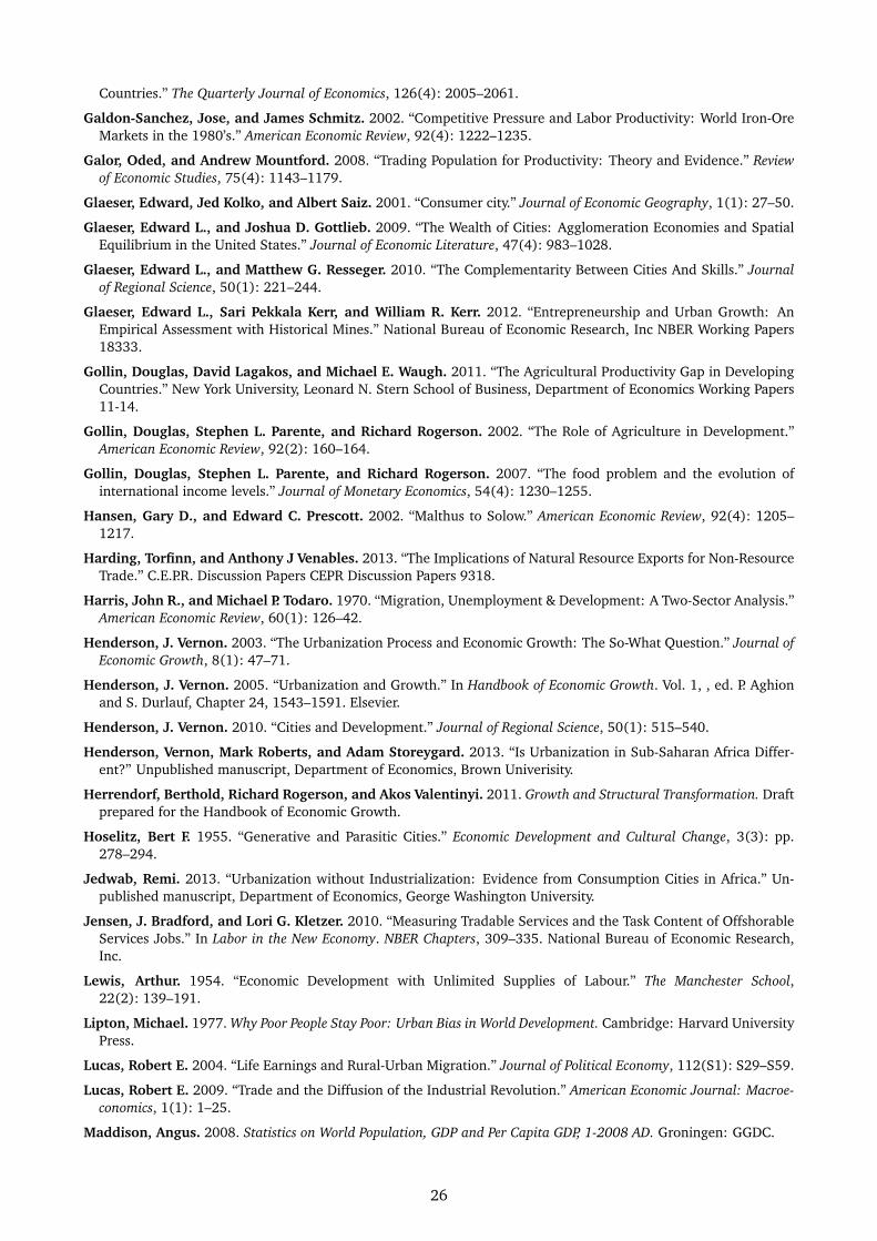
Countries.” The Quarterly Journal of Economics, 126(4): 2005–2061.

Galdon-Sanchez, Jose, and James Schmitz. 2002. “Competitive Pressure and Labor Productivity: World Iron-OreMarkets in the 1980’s.” American Economic Review, 92(4): 1222–1235.

Galor, Oded, and Andrew Mountford. 2008. “Trading Population for Productivity: Theory and Evidence.” Reviewof Economic Studies, 75(4): 1143–1179.

Glaeser, Edward, Jed Kolko, and Albert Saiz. 2001. “Consumer city.” Journal of Economic Geography, 1(1): 27–50.

Glaeser, Edward L., and Joshua D. Gottlieb. 2009. “The Wealth of Cities: Agglomeration Economies and SpatialEquilibrium in the United States.” Journal of Economic Literature, 47(4): 983–1028.

Glaeser, Edward L., and Matthew G. Resseger. 2010. “The Complementarity Between Cities And Skills.” Journalof Regional Science, 50(1): 221–244.

Glaeser, Edward L., Sari Pekkala Kerr, and William R. Kerr. 2012. “Entrepreneurship and Urban Growth: AnEmpirical Assessment with Historical Mines.” National Bureau of Economic Research, Inc NBER Working Papers18333.

Gollin, Douglas, David Lagakos, and Michael E. Waugh. 2011. “The Agricultural Productivity Gap in DevelopingCountries.” New York University, Leonard N. Stern School of Business, Department of Economics Working Papers11-14.

Gollin, Douglas, Stephen L. Parente, and Richard Rogerson. 2002. “The Role of Agriculture in Development.”American Economic Review, 92(2): 160–164.

Gollin, Douglas, Stephen L. Parente, and Richard Rogerson. 2007. “The food problem and the evolution ofinternational income levels.” Journal of Monetary Economics, 54(4): 1230–1255.

Hansen, Gary D., and Edward C. Prescott. 2002. “Malthus to Solow.” American Economic Review, 92(4): 1205–1217.

Harding, Torfinn, and Anthony J Venables. 2013. “The Implications of Natural Resource Exports for Non-ResourceTrade.” C.E.P.R. Discussion Papers CEPR Discussion Papers 9318.

Harris, John R., and Michael P. Todaro. 1970. “Migration, Unemployment & Development: A Two-Sector Analysis.”American Economic Review, 60(1): 126–42.

Henderson, J. Vernon. 2003. “The Urbanization Process and Economic Growth: The So-What Question.” Journal ofEconomic Growth, 8(1): 47–71.

Henderson, J. Vernon. 2005. “Urbanization and Growth.” In Handbook of Economic Growth. Vol. 1, , ed. P. Aghionand S. Durlauf, Chapter 24, 1543–1591. Elsevier.

Henderson, J. Vernon. 2010. “Cities and Development.” Journal of Regional Science, 50(1): 515–540.

Henderson, Vernon, Mark Roberts, and Adam Storeygard. 2013. “Is Urbanization in Sub-Saharan Africa Differ-ent?” Unpublished manuscript, Department of Economics, Brown Univerisity.

Herrendorf, Berthold, Richard Rogerson, and Akos Valentinyi. 2011. Growth and Structural Transformation. Draftprepared for the Handbook of Economic Growth.

Hoselitz, Bert F. 1955. “Generative and Parasitic Cities.” Economic Development and Cultural Change, 3(3): pp.278–294.

Jedwab, Remi. 2013. “Urbanization without Industrialization: Evidence from Consumption Cities in Africa.” Un-published manuscript, Department of Economics, George Washington University.

Jensen, J. Bradford, and Lori G. Kletzer. 2010. “Measuring Tradable Services and the Task Content of OffshorableServices Jobs.” In Labor in the New Economy. NBER Chapters, 309–335. National Bureau of Economic Research,Inc.

Lewis, Arthur. 1954. “Economic Development with Unlimited Supplies of Labour.” The Manchester School,22(2): 139–191.

Lipton, Michael. 1977. Why Poor People Stay Poor: Urban Bias in World Development. Cambridge: Harvard UniversityPress.

Lucas, Robert E. 2004. “Life Earnings and Rural-Urban Migration.” Journal of Political Economy, 112(S1): S29–S59.

Lucas, Robert E. 2009. “Trade and the Diffusion of the Industrial Revolution.” American Economic Journal: Macroe-conomics, 1(1): 1–25.

Maddison, Angus. 2008. Statistics on World Population, GDP and Per Capita GDP, 1-2008 AD. Groningen: GGDC.

26

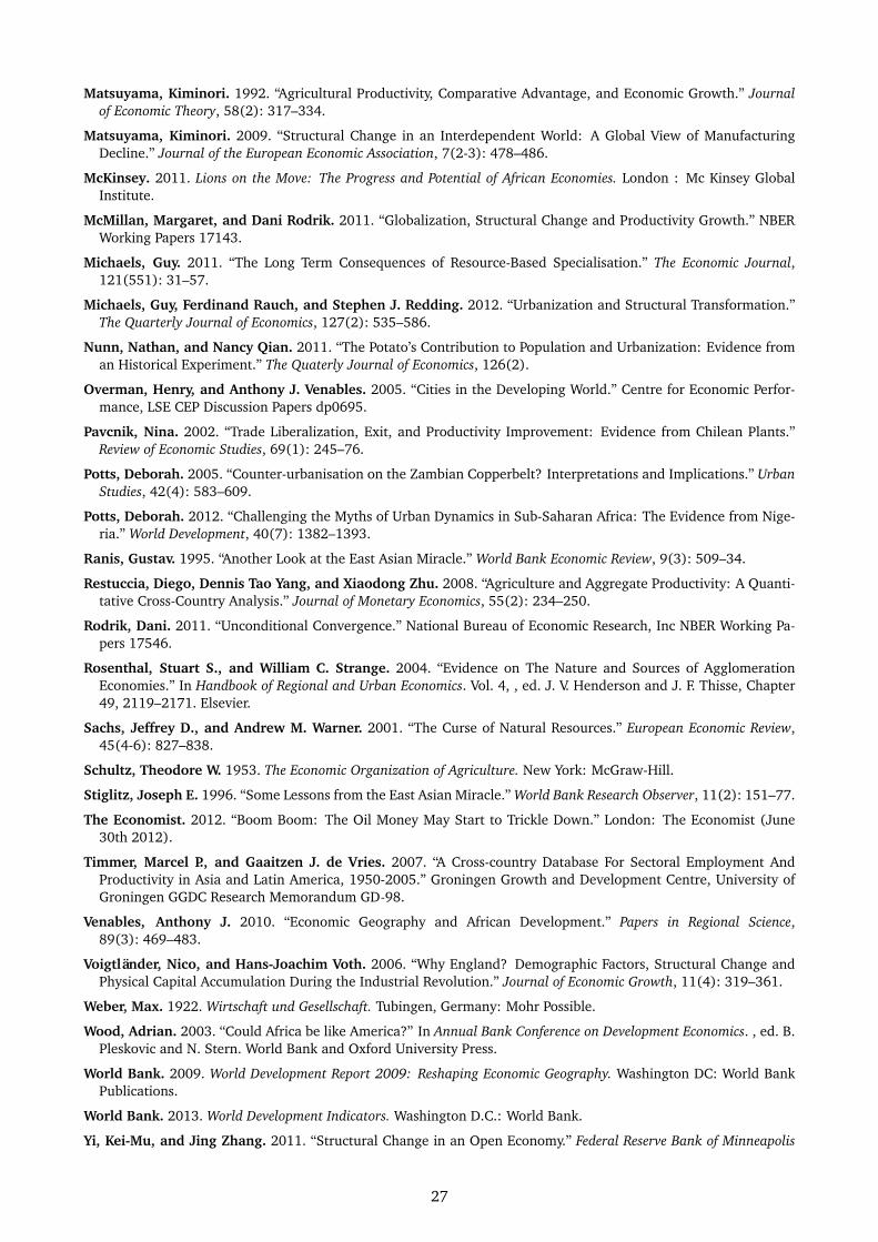
Matsuyama, Kiminori. 1992. “Agricultural Productivity, Comparative Advantage, and Economic Growth.” Journalof Economic Theory, 58(2): 317–334.

Matsuyama, Kiminori. 2009. “Structural Change in an Interdependent World: A Global View of ManufacturingDecline.” Journal of the European Economic Association, 7(2-3): 478–486.

McKinsey. 2011. Lions on the Move: The Progress and Potential of African Economies. London : Mc Kinsey GlobalInstitute.

McMillan, Margaret, and Dani Rodrik. 2011. “Globalization, Structural Change and Productivity Growth.” NBERWorking Papers 17143.

Michaels, Guy. 2011. “The Long Term Consequences of Resource-Based Specialisation.” The Economic Journal,121(551): 31–57.

Michaels, Guy, Ferdinand Rauch, and Stephen J. Redding. 2012. “Urbanization and Structural Transformation.”The Quarterly Journal of Economics, 127(2): 535–586.

Nunn, Nathan, and Nancy Qian. 2011. “The Potato’s Contribution to Population and Urbanization: Evidence froman Historical Experiment.” The Quaterly Journal of Economics, 126(2).

Overman, Henry, and Anthony J. Venables. 2005. “Cities in the Developing World.” Centre for Economic Perfor-mance, LSE CEP Discussion Papers dp0695.

Pavcnik, Nina. 2002. “Trade Liberalization, Exit, and Productivity Improvement: Evidence from Chilean Plants.”Review of Economic Studies, 69(1): 245–76.

Potts, Deborah. 2005. “Counter-urbanisation on the Zambian Copperbelt? Interpretations and Implications.” UrbanStudies, 42(4): 583–609.

Potts, Deborah. 2012. “Challenging the Myths of Urban Dynamics in Sub-Saharan Africa: The Evidence from Nige-ria.” World Development, 40(7): 1382–1393.

Ranis, Gustav. 1995. “Another Look at the East Asian Miracle.” World Bank Economic Review, 9(3): 509–34.

Restuccia, Diego, Dennis Tao Yang, and Xiaodong Zhu. 2008. “Agriculture and Aggregate Productivity: A Quanti-tative Cross-Country Analysis.” Journal of Monetary Economics, 55(2): 234–250.

Rodrik, Dani. 2011. “Unconditional Convergence.” National Bureau of Economic Research, Inc NBER Working Pa-pers 17546.

Rosenthal, Stuart S., and William C. Strange. 2004. “Evidence on The Nature and Sources of AgglomerationEconomies.” In Handbook of Regional and Urban Economics. Vol. 4, , ed. J. V. Henderson and J. F. Thisse, Chapter49, 2119–2171. Elsevier.

Sachs, Jeffrey D., and Andrew M. Warner. 2001. “The Curse of Natural Resources.” European Economic Review,45(4-6): 827–838.

Schultz, Theodore W. 1953. The Economic Organization of Agriculture. New York: McGraw-Hill.

Stiglitz, Joseph E. 1996. “Some Lessons from the East Asian Miracle.” World Bank Research Observer, 11(2): 151–77.

The Economist. 2012. “Boom Boom: The Oil Money May Start to Trickle Down.” London: The Economist (June30th 2012).

Timmer, Marcel P., and Gaaitzen J. de Vries. 2007. “A Cross-country Database For Sectoral Employment AndProductivity in Asia and Latin America, 1950-2005.” Groningen Growth and Development Centre, University ofGroningen GGDC Research Memorandum GD-98.

Venables, Anthony J. 2010. “Economic Geography and African Development.” Papers in Regional Science,89(3): 469–483.

Voigtländer, Nico, and Hans-Joachim Voth. 2006. “Why England? Demographic Factors, Structural Change andPhysical Capital Accumulation During the Industrial Revolution.” Journal of Economic Growth, 11(4): 319–361.

Weber, Max. 1922. Wirtschaft und Gesellschaft. Tubingen, Germany: Mohr Possible.

Wood, Adrian. 2003. “Could Africa be like America?” In Annual Bank Conference on Development Economics. , ed. B.Pleskovic and N. Stern. World Bank and Oxford University Press.

World Bank. 2009. World Development Report 2009: Reshaping Economic Geography. Washington DC: World BankPublications.

World Bank. 2013. World Development Indicators. Washington D.C.: World Bank.

Yi, Kei-Mu, and Jing Zhang. 2011. “Structural Change in an Open Economy.” Federal Reserve Bank of Minneapolis

27

Staff Report, 456.

Young, Alwyn. 2012. “The African Growth Miracle.” Journal of Political Economy, 120(4): 696 – 739.

28

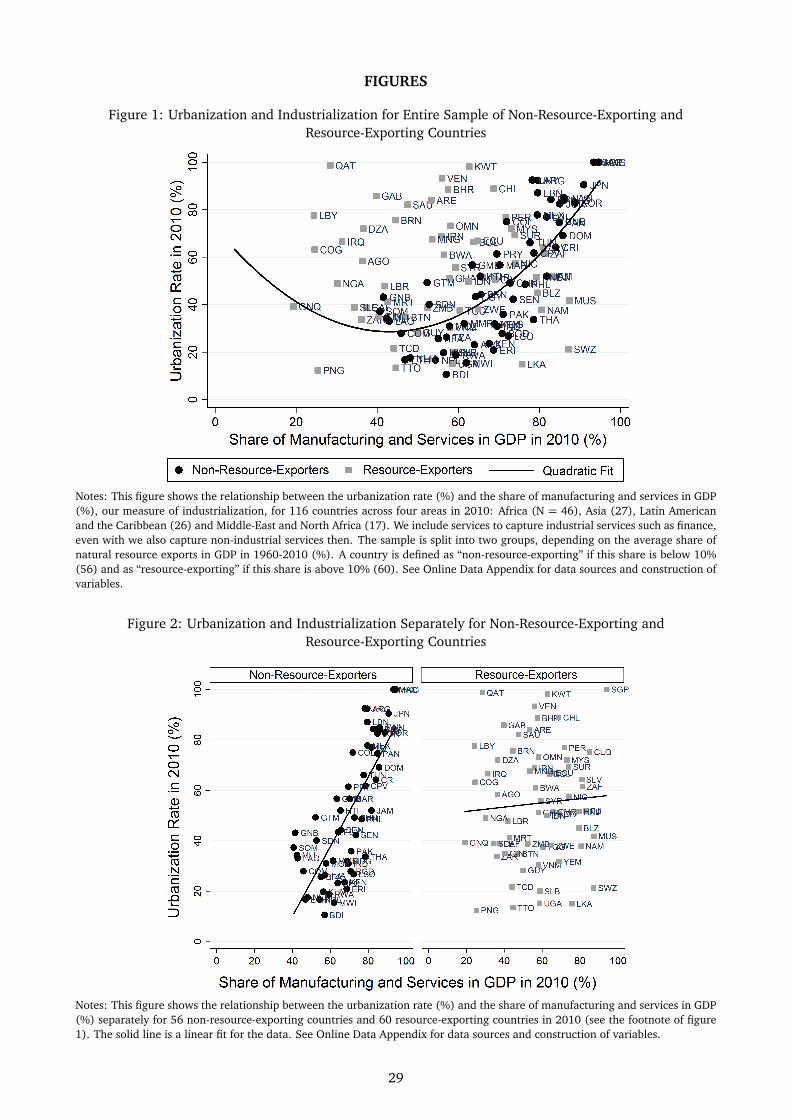
FIGURES

Figure 1: Urbanization and Industrialization for Entire Sample of Non-Resource-Exporting andResource-Exporting Countries

Notes: This figure shows the relationship between the urbanization rate (%) and the share of manufacturing and services in GDP(%), our measure of industrialization, for 116 countries across four areas in 2010: Africa (N = 46), Asia (27), Latin Americanand the Caribbean (26) and Middle-East and North Africa (17). We include services to capture industrial services such as finance,even with we also capture non-industrial services then. The sample is split into two groups, depending on the average share ofnatural resource exports in GDP in 1960-2010 (%). A country is defined as “non-resource-exporting” if this share is below 10%(56) and as “resource-exporting” if this share is above 10% (60). See Online Data Appendix for data sources and construction ofvariables.

Figure 2: Urbanization and Industrialization Separately for Non-Resource-Exporting andResource-Exporting Countries

Notes: This figure shows the relationship between the urbanization rate (%) and the share of manufacturing and services in GDP(%) separately for 56 non-resource-exporting countries and 60 resource-exporting countries in 2010 (see the footnote of figure1). The solid line is a linear fit for the data. See Online Data Appendix for data sources and construction of variables.

29

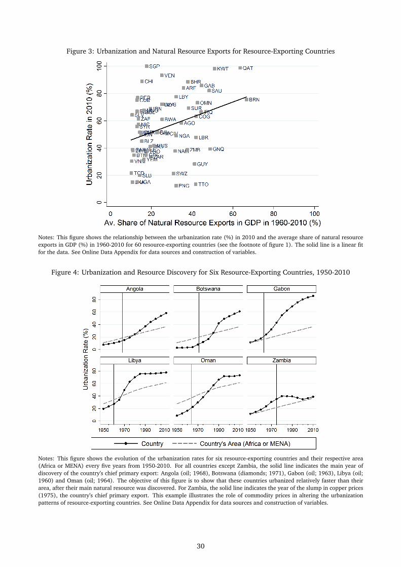
Figure 3: Urbanization and Natural Resource Exports for Resource-Exporting Countries

Notes: This figure shows the relationship between the urbanization rate (%) in 2010 and the average share of natural resourceexports in GDP (%) in 1960-2010 for 60 resource-exporting countries (see the footnote of figure 1). The solid line is a linear fitfor the data. See Online Data Appendix for data sources and construction of variables.

Figure 4: Urbanization and Resource Discovery for Six Resource-Exporting Countries, 1950-2010

Notes: This figure shows the evolution of the urbanization rates for six resource-exporting countries and their respective area(Africa or MENA) every five years from 1950-2010. For all countries except Zambia, the solid line indicates the main year ofdiscovery of the country’s chief primary export: Angola (oil; 1968), Botswana (diamonds; 1971), Gabon (oil; 1963), Libya (oil;1960) and Oman (oil; 1964). The objective of this figure is to show that these countries urbanized relatively faster than theirarea, after their main natural resource was discovered. For Zambia, the solid line indicates the year of the slump in copper prices(1975), the country’s chief primary export. This example illustrates the role of commodity prices in altering the urbanizationpatterns of resource-exporting countries. See Online Data Appendix for data sources and construction of variables.

30

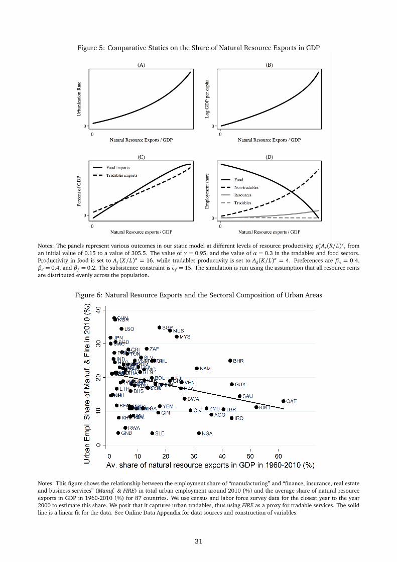
Figure 5: Comparative Statics on the Share of Natural Resource Exports in GDP

Notes: The panels represent various outcomes in our static model at different levels of resource productivity, p∗r Ar(R/L)γ, froman initial value of 0.15 to a value of 305.5. The value of γ = 0.95, and the value of α = 0.3 in the tradables and food sectors.Productivity in food is set to A f (X/L)α = 16, while tradables productivity is set to Ad(K/L)α = 4. Preferences are βn = 0.4,βd = 0.4, and β f = 0.2. The subsistence constraint is c f = 15. The simulation is run using the assumption that all resource rentsare distributed evenly across the population.

Figure 6: Natural Resource Exports and the Sectoral Composition of Urban Areas

Notes: This figure shows the relationship between the employment share of “manufacturing” and “finance, insurance, real estateand business services” (Manuf. & FIRE) in total urban employment around 2010 (%) and the average share of natural resourceexports in GDP in 1960-2010 (%) for 87 countries. We use census and labor force survey data for the closest year to the year2000 to estimate this share. We posit that it captures urban tradables, thus using FIRE as a proxy for tradable services. The solidline is a linear fit for the data. See Online Data Appendix for data sources and construction of variables.

31

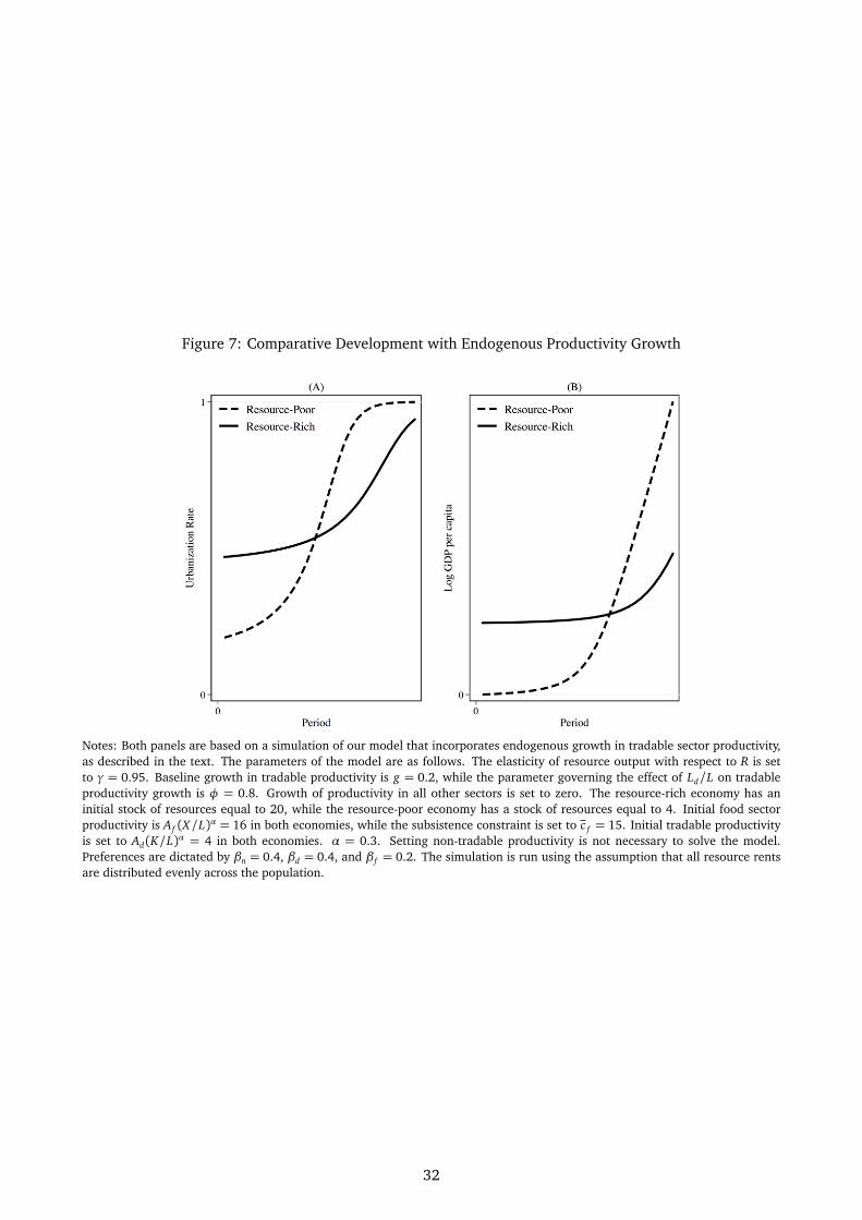
Figure 7: Comparative Development with Endogenous Productivity Growth

Notes: Both panels are based on a simulation of our model that incorporates endogenous growth in tradable sector productivity,as described in the text. The parameters of the model are as follows. The elasticity of resource output with respect to R is setto γ = 0.95. Baseline growth in tradable productivity is g = 0.2, while the parameter governing the effect of Ld/L on tradableproductivity growth is φ = 0.8. Growth of productivity in all other sectors is set to zero. The resource-rich economy has aninitial stock of resources equal to 20, while the resource-poor economy has a stock of resources equal to 4. Initial food sectorproductivity is A f (X/L)α = 16 in both economies, while the subsistence constraint is set to c f = 15. Initial tradable productivityis set to Ad(K/L)α = 4 in both economies. α = 0.3. Setting non-tradable productivity is not necessary to solve the model.Preferences are dictated by βn = 0.4, βd = 0.4, and β f = 0.2. The simulation is run using the assumption that all resource rentsare distributed evenly across the population.

32

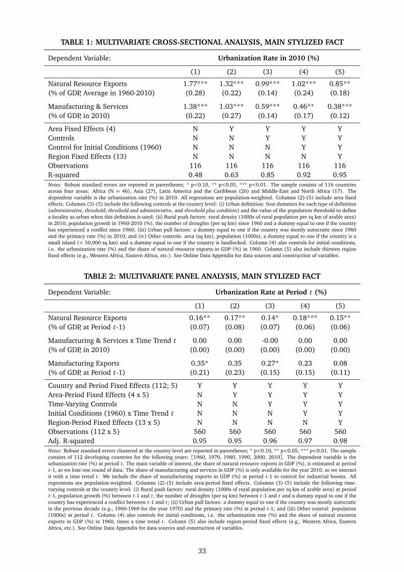
TABLE 1: MULTIVARIATE CROSS-SECTIONAL ANALYSIS, MAIN STYLIZED FACT

Dependent Variable: Urbanization Rate in 2010 (%)

(1) (2) (3) (4) (5)

Natural Resource Exports 1.77*** 1.32*** 0.99*** 1.02*** 0.85**(% of GDP, Average in 1960-2010) (0.28) (0.22) (0.14) (0.24) (0.18)

Manufacturing & Services 1.38*** 1.03*** 0.59*** 0.46** 0.38***(% of GDP, in 2010) (0.22) (0.27) (0.14) (0.17) (0.12)

Area Fixed Effects (4) N Y Y Y YControls N N Y Y YControl for Initial Conditions (1960) N N N Y YRegion Fixed Effects (13) N N N N YObservations 116 116 116 116 116R-squared 0.48 0.63 0.85 0.92 0.95Notes: Robust standard errors are reported in parentheses; * p<0.10, ** p<0.05, *** p<0.01. The sample consists of 116 countriesacross four areas: Africa (N = 46), Asia (27), Latin America and the Caribbean (26) and Middle-East and North Africa (17). Thedependent variable is the urbanization rate (%) in 2010. All regressions are population-weighted. Columns (2)-(5) include area fixedeffects. Columns (3)-(5) include the following controls at the country level: (i) Urban definition: four dummies for each type of definition(administrative, threshold, threshold and administrative, and threshold plus condition) and the value of the population threshold to definea locality as urban when this definition is used; (ii) Rural push factors: rural density (1000s of rural population per sq km of arable area)in 2010, population growth in 1960-2010 (%), the number of droughts (per sq km) since 1960 and a dummy equal to one if the countryhas experienced a conflict since 1960; (iii) Urban pull factors: a dummy equal to one if the country was mostly autocratic since 1960and the primacy rate (%) in 2010; and (iv) Other controls: area (sq km), population (1000s), a dummy equal to one if the country is asmall island (< 50,000 sq km) and a dummy equal to one if the country is landlocked. Column (4) also controls for initial conditions,i.e. the urbanization rate (%) and the share of natural resource exports in GDP (%) in 1960. Column (5) also include thirteen regionfixed effects (e.g., Western Africa, Eastern Africa, etc.). See Online Data Appendix for data sources and construction of variables.

TABLE 2: MULTIVARIATE PANEL ANALYSIS, MAIN STYLIZED FACT

Dependent Variable: Urbanization Rate at Period t (%)

(1) (2) (3) (4) (5)

Natural Resource Exports 0.16** 0.17** 0.14* 0.18*** 0.15**(% of GDP, at Period t-1) (0.07) (0.08) (0.07) (0.06) (0.06)

Manufacturing & Services x Time Trend t 0.00 0.00 -0.00 0.00 0.00(% of GDP, in 2010) (0.00) (0.00) (0.00) (0.00) (0.00)

Manufacturing Exports 0.35* 0.35 0.27* 0.23 0.08(% of GDP, at Period t-1) (0.21) (0.23) (0.15) (0.15) (0.11)

Country and Period Fixed Effects (112; 5) Y Y Y Y YArea-Period Fixed Effects (4 x 5) N Y Y Y YTime-Varying Controls N N Y Y YInitial Conditions (1960) x Time Trend t N N N Y YRegion-Period Fixed Effects (13 x 5) N N N N YObservations (112 x 5) 560 560 560 560 560Adj. R-squared 0.95 0.95 0.96 0.97 0.98Notes: Robust standard errors clustered at the country level are reported in parentheses; * p<0.10, ** p<0.05, *** p<0.01. The sampleconsists of 112 developing countries for the following years: [1960, 1970, 1980, 1990, 2000, 2010]. The dependent variable is theurbanization rate (%) at period t. The main variable of interest, the share of natural resource exports in GDP (%), is estimated at periodt-1, so we lose one round of data. The share of manufacturing and services in GDP (%) is only available for the year 2010, so we interactit with a time trend t. We include the share of manufacturing exports in GDP (%) at period t-1 to control for industrial booms. Allregressions are population-weighted. Columns (2)-(5) include area-period fixed effects. Columns (3)-(5) include the following time-varying controls at the country level: (i) Rural push factors: rural density (1000s of rural population per sq km of arable area) at periodt-1, population growth (%) between t-1 and t, the number of droughts (per sq km) between t-1 and t and a dummy equal to one if thecountry has experienced a conflict between t-1 and t; (ii) Urban pull factors: a dummy equal to one if the country was mostly autocraticin the previous decade (e.g., 1960-1969 for the year 1970) and the primacy rate (%) at period t-1; and (iii) Other control: population(1000s) at period t. Column (4) also controls for initial conditions, i.e. the urbanization rate (%) and the share of natural resourceexports in GDP (%) in 1960, times a time trend t. Column (5) also include region-period fixed effects (e.g., Western Africa, EasternAfrica, etc.). See Online Data Appendix for data sources and construction of variables.

33

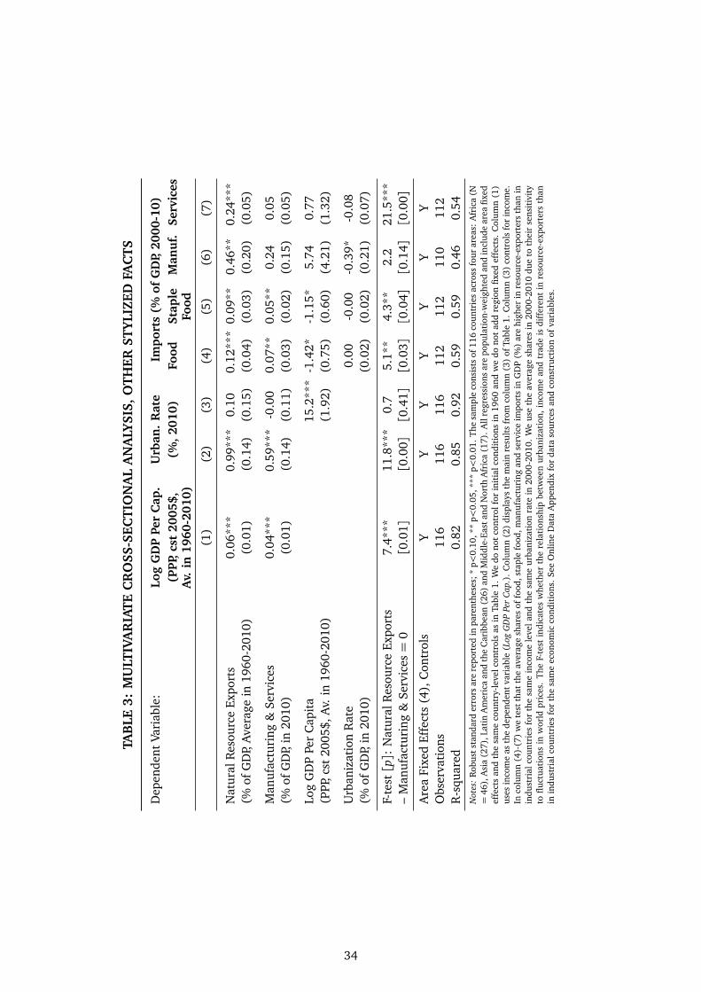
TAB

LE3:

MU

LTIV

AR

IAT

EC

RO

SS-S

ECT

ION

AL

AN

ALY

SIS,

OT

HER

STY

LIZE

DFA

CT

S

Dep

ende

ntVa

riab

le:

Log

GD

PPe

rC

ap.

Urb

an.

Rat

eIm

port

s(%

ofG

DP,

2000

-10)

(PPP

,cst

2005

$,(%

,201

0)Fo

odSt

aple

Man

uf.

Serv

ices

Av.

in19

60-2

010)

Food

(1)

(2)

(3)

(4)

(5)

(6)

(7)

Nat

ural

Res

ourc

eEx

port

s0.

06**

*0.

99**

*0.

100.

12**

*0.

09**

0.46

**0.

24**

*(%

ofG

DP,

Ave

rage

in19

60-2

010)

(0.0

1)(0

.14)

(0.1

5)(0

.04)

(0.0

3)(0

.20)

(0.0

5)

Man

ufac

turi

ng&

Serv

ices

0.04

***

0.59

***

-0.0

00.

07**

0.05

**0.

240.

05(%

ofG

DP,

in20

10)

(0.0

1)(0

.14)

(0.1

1)(0

.03)

(0.0

2)(0

.15)

(0.0

5)

Log

GD

PPe

rC

apit

a15

.2**

*-1

.42*

-1.1

5*5.

740.

77(P

PP,c

st20

05$,

Av.

in19

60-2

010)

(1.9

2)(0

.75)

(0.6

0)(4

.21)

(1.3

2)

Urb

aniz

atio

nR

ate

0.00

-0.0

0-0

.39*

-0.0

8(%

ofG

DP,

in20

10)

(0.0

2)(0

.02)

(0.2

1)(0

.07)

F-te

st[p]:

Nat

ural

Res

ourc

eEx

port

s7.

4***

11.8

***

0.7

5.1*

*4.

3**

2.2

21.5

***

–M

anuf

actu

ring

&Se

rvic

es=

0[0

.01]

[0.0

0][0

.41]

[0.0

3][0

.04]

[0.1

4][0

.00]

Are

aFi

xed

Effe

cts

(4),

Con

trol

sY

YY

YY

YY

Obs

erva

tion

s11

611

611

611

211

211

011

2R

-squ

ared

0.82

0.85

0.92

0.59

0.59

0.46

0.54

Not

es:

Rob

usts

tand

ard

erro

rsar

ere

port

edin

pare

nthe

ses;

*p<

0.10

,**

p<0.

05,*

**p<

0.01

.Th

esa

mpl

eco

nsis

tsof

116

coun

trie

sac

ross

four

area

s:A

fric

a(N

=46

),A

sia

(27)

,Lat

inA

mer

ica

and

the

Car

ibbe

an(2

6)an

dM

iddl

e-Ea

stan

dN

orth

Afr

ica

(17)

.A

llre

gres

sion

sar

epo

pula

tion

-wei

ghte

dan

din

clud

ear

eafix

edef

fect

san

dth

esa

me

coun

try-

leve

lcon

trol

sas

inTa

ble

1.W

edo

not

cont

rolf

orin

itia

lcon

diti

ons

in19

60an

dw

edo

not

add

regi

onfix

edef

fect

s.C

olum

n(1

)us

esin

com

eas

the

depe

nden

tvar

iabl

e(L

ogG

DP

Per

Cap.

).C

olum

n(2

)di

spla

ysth

em

ain

resu

lts

from

colu

mn

(3)

ofTa

ble

1.C

olum

n(3

)co

ntro

lsfo

rin

com

e.In

colu

mn

(4)-

(7)

we

test

that

the

aver

age

shar

esof

food

,sta

ple

food

,man

ufac

turi

ngan

dse

rvic

eim

port

sin

GD

P(%

)ar

ehi

gher

inre

sour

ce-e

xpor

ters

than

inin

dust

rial

coun

trie

sfo

rth

esa

me

inco

me

leve

land

the

sam

eur

bani

zati

onra

tein

2000

-201

0.W

eus

eth

eav

erag

esh

ares

in20

00-2

010

due

toth

eir

sens

itiv

ity

toflu

ctua

tion

sin

wor

ldpr

ices

.Th

eF-

test

indi

cate

sw

heth

erth

ere

lati

onsh

ipbe

twee

nur

bani

zati

on,i

ncom

ean

dtr

ade

isdi

ffer

ent

inre

sour

ce-e

xpor

ters

than

inin

dust

rial

coun

trie

sfo

rth

esa

me

econ

omic

cond

itio

ns.

See

Onl

ine

Dat

aA

ppen

dix

for

data

sour

ces

and

cons

truc

tion

ofva

riab

les.

34

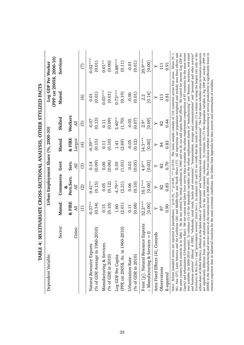
TAB

LE4:

MU

LTIV

AR

IAT

EC

RO

SS-S

ECT

ION

AL

AN

ALY

SIS,

OT

HER

STY

LIZE

DFA

CT

S

Dep

ende

ntVa

riab

le:

Urb

anEm

ploy

men

tSh

are

(%,2

000-

10)

Log

GD

PPe

rW

orke

r(P

PPcs

t20

05$,

2000

-10)

Sect

or:

Man

uf.

Com

mer

ce&

Gov

tM

anu

f.Sk

ille

dM

anu

f.Se

rvic

es

&FI

RE

Pers

.Ser

v.Se

rv.

&FI

RE

Wor

kers

Cit

ies:

All

All

All

Larg

est

All

(1)

(2)

(3)

(4)

(5)

(6)

(7)

Nat

ural

Res

ourc

eEx

port

s-0

.37*

*0.

41**

0.14

-0.3

9**

-0.0

70.

01-0

.02*

**(%

ofG

DP,

Ave

rage

in19

60-2

010)

(0.1

4)(0

.15)

(0.0

9)(0

.15)

(0.1

3)(0

.01)

(0.0

1)

Man

ufac

turi

ng&

Serv

ices

0.15

0.05

0.00

0.11

0.11

0.03

***

0.01

**(%

ofG

DP,

in20

10)

(0.1

0)(0

.12)

(0.0

6)(0

.10)

(0.0

9)(0

.01)

(0.0

0)

Log

GD

PPe

rC

apit

a1.

60-4

.79*

*0.

591.

413.

40**

0.73

***

0.88

***

(PPP

,cst

2005

$,A

v.in

1960

-201

0)(2

.01)

(2.2

1)(1

.01)

(2.6

9)(1

.70)

(0.1

9)(0

.11)

Urb

aniz

atio

nR

ate

0.11

0.06

-0.0

1-0

.05

-0.0

5-0

.00

-0.0

1(%

ofG

DP,

in20

10)

(0.0

8)(0

.10)

(0.0

5)(0

.12)

(0.0

7)(0

.01)

(0.0

1)

F-te

st[p]:

Nat

ural

Res

ourc

eEx

port

s32

.2**

*10

.1**

*4.

9**

14.3

***

2.9*

2.2

20.9

***

–M

anuf

actu

ring

&Se

rvic

es=

0[0

.00]

[0.0

0][0

.03]

[0.0

0][0

.09]

[0.1

4][0

.00]

Are

aFi

xed

Effe

cts

(4),

Con

trol

sY

YY

YY

YY

Obs

erva

tion

s87

8282

8482

111

111

R-s

quar

ed0.

900.

830.

700.

830.

440.

810.

91N

otes

:R

obus

tst

anda

rder

rors

are

repo

rted

inpa

rent

hese

s;*

p<0.

10,

**p<

0.05

,**

*p<

0.01

.Th

em

ain

sam

ple

cons

ists

of11

6co

untr

ies

acro

ssfo

urar

eas:

Afr

ica

(N=

46),

Asi

a(2

7),

Lati

nA

mer

ica

and

the

Car

ibbe

an(2

6)an

dM

iddl

e-Ea

stan

dN

orth

Afr

ica

(17)

.A

llre

gres

sion

sar

epo

pula

tion

-wei

ghte

dan

din

clud

ear

eafix

edef

fect

san

dth

esa

me

coun

try-

leve

lco

ntro

lsas

inTa

ble

1.W

edo

not

cont

rol

for

init

ial

cond

itio

nsin

1960

and

we

dono

tad

dre

gion

fixed

effe

cts.

We

cont

rol

for

inco

me

(Log

GD

PPe

rCa

pita

)an

dur

bani

zati

on(U

rban

izat

ion

Rate

).W

eus

ece

nsus

and

labo

rfo

rce

surv

eyda

tato

exam

ine

the

urba

nem

ploy

men

tco

mpo

siti

onof

87co

untr

ies

for

the

mos

tre

cent

year

avai

labl

e(i

n20

00-2

010

mos

tly)

.In

colu

mns

(1)-

(3)

the

depe

nden

tva

riab

les

are

the

urba

nem

ploy

men

tsh

ares

of“m

anuf

actu

ring

”an

d“fi

nanc

e,in

sura

nce,

real

esta

tean

dbu

sine

ssse

rvic

es”

(Man

uf.

&FI

RE),

“who

lesa

le,

reta

iltr

ade,

hote

lsan

dre

stau

rant

s”,

“tra

nspo

rtat

ion,

stor

age

and

com

mun

icat

ions

”an

d“p

erso

nal

and

othe

rse

rvic

es”

(Com

mer

ce&

Pers

.Ser

v.)

and

“gov

ernm

ent

serv

ices

”(G

ovt

Serv

.).

Inco

lum

ns(4

)an

d(5

)w

eve

rify

that

the

resu

ltof

colu

mn

(1)

isro

bust

tous

ing

the

larg

est

city

only

orth

eur

ban

shar

eof

Skill

edW

orke

rs,d

efine

das

the

labo

rsh

are

of“p

rofe

ssio

nals

”an

d“t

echn

icia

nsan

das

soci

ate

prof

essi

onal

s”.

The

F-te

stsh

ows

whe

ther

citi

esin

reso

urce

-exp

orte

rsar

esi

gnifi

cant

lydi

ffer

ent

from

citi

esin

indu

stri

alco

untr

ies

for

the

sam

eec

onom

icco

ndit

ions

.In

colu

mns

(6)-

(7)

the

depe

nden

tva

riab

leis

log

GD

Ppe

rw

orke

r(P

PPcs

t20

05$)

inth

em

anuf

actu

ring

and

serv

ice

sect

ors

atth

ena

tion

alle

veli

n20

00-2

010.

The

F-te

stin

dica

tes

whe

ther

man

ufac

turi

ngor

serv

ice

prod

ucti

vity

issi

gnifi

cant

lylo

wer

inre

sour

ce-e

xpor

ters

than

inin

dust

rial

coun

trie

sfo

rth

esa

me

econ

omic

cond

itio

ns.

See

Onl

ine

Dat

aA

ppen

dix

for

data

sour

ces

and

cons

truc

tion

ofva

riab

les.

35

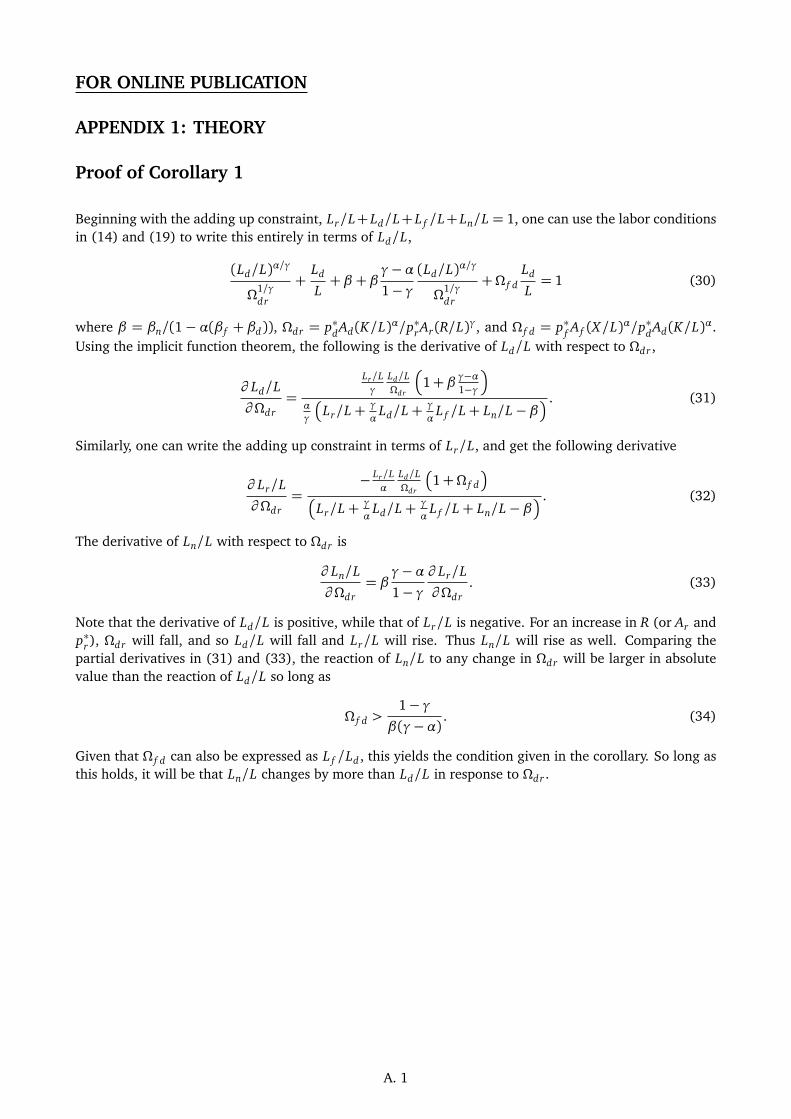
FOR ONLINE PUBLICATION

APPENDIX 1: THEORY

Proof of Corollary 1

Beginning with the adding up constraint, Lr/L+ Ld/L+ L f /L+ Ln/L = 1, one can use the labor conditionsin (14) and (19) to write this entirely in terms of Ld/L,

(Ld/L)α/γ

Ω1/γdr

+Ld

L+ β + β

γ−α1− γ

(Ld/L)α/γ

Ω1/γdr

+Ω f dLd

L= 1 (30)

where β = βn/(1− α(β f + βd)), Ωdr = p∗dAd(K/L)α/p∗rAr(R/L)γ, and Ω f d = p∗f A f (X/L)α/p∗dAd(K/L)α.Using the implicit function theorem, the following is the derivative of Ld/L with respect to Ωdr ,

∂ Ld/L

∂Ωdr=

Lr/Lγ

Ld/LΩdr

1+ β γ−α1−γ

αγ

Lr/L+ γ

αLd/L+ γ

αL f /L+ Ln/L− β

. (31)

Similarly, one can write the adding up constraint in terms of Lr/L, and get the following derivative

∂ Lr/L

∂Ωdr=

− Lr/Lα

Ld/LΩdr

1+Ω f d

Lr/L+ γ

αLd/L+ γ

αL f /L+ Ln/L− β

. (32)

The derivative of Ln/L with respect to Ωdr is

∂ Ln/L

∂Ωdr= β

γ−α1− γ

∂ Lr/L

∂Ωdr. (33)

Note that the derivative of Ld/L is positive, while that of Lr/L is negative. For an increase in R (or Ar andp∗r), Ωdr will fall, and so Ld/L will fall and Lr/L will rise. Thus Ln/L will rise as well. Comparing thepartial derivatives in (31) and (33), the reaction of Ln/L to any change in Ωdr will be larger in absolutevalue than the reaction of Ld/L so long as

Ω f d >1− γβ(γ−α)

. (34)

Given that Ω f d can also be expressed as L f /Ld , this yields the condition given in the corollary. So long asthis holds, it will be that Ln/L changes by more than Ld/L in response to Ωdr .

A. 1

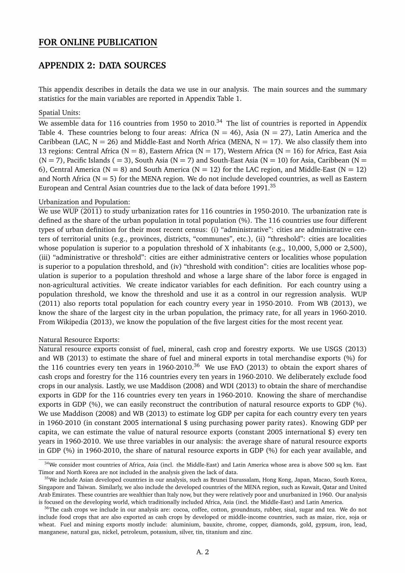
FOR ONLINE PUBLICATION

APPENDIX 2: DATA SOURCES

This appendix describes in details the data we use in our analysis. The main sources and the summarystatistics for the main variables are reported in Appendix Table 1.

Spatial Units:

We assemble data for 116 countries from 1950 to 2010.34 The list of countries is reported in AppendixTable 4. These countries belong to four areas: Africa (N = 46), Asia (N = 27), Latin America and theCaribbean (LAC, N = 26) and Middle-East and North Africa (MENA, N = 17). We also classify them into13 regions: Central Africa (N = 8), Eastern Africa (N = 17), Western Africa (N = 16) for Africa, East Asia(N = 7), Pacific Islands ( = 3), South Asia (N = 7) and South-East Asia (N = 10) for Asia, Caribbean (N =6), Central America (N = 8) and South America (N = 12) for the LAC region, and Middle-East (N = 12)and North Africa (N = 5) for the MENA region. We do not include developed countries, as well as EasternEuropean and Central Asian countries due to the lack of data before 1991.35

Urbanization and Population:We use WUP (2011) to study urbanization rates for 116 countries in 1950-2010. The urbanization rate isdefined as the share of the urban population in total population (%). The 116 countries use four differenttypes of urban definition for their most recent census: (i) “administrative”: cities are administrative cen-ters of territorial units (e.g., provinces, districts, “communes”, etc.), (ii) “threshold”: cities are localitieswhose population is superior to a population threshold of X inhabitants (e.g., 10,000, 5,000 or 2,500),(iii) “administrative or threshold”: cities are either administrative centers or localities whose populationis superior to a population threshold, and (iv) “threshold with condition”: cities are localities whose pop-ulation is superior to a population threshold and whose a large share of the labor force is engaged innon-agricultural activities. We create indicator variables for each definition. For each country using apopulation threshold, we know the threshold and use it as a control in our regression analysis. WUP(2011) also reports total population for each country every year in 1950-2010. From WB (2013), weknow the share of the largest city in the urban population, the primacy rate, for all years in 1960-2010.From Wikipedia (2013), we know the population of the five largest cities for the most recent year.

Natural Resource Exports:Natural resource exports consist of fuel, mineral, cash crop and forestry exports. We use USGS (2013)and WB (2013) to estimate the share of fuel and mineral exports in total merchandise exports (%) forthe 116 countries every ten years in 1960-2010.36 We use FAO (2013) to obtain the export shares ofcash crops and forestry for the 116 countries every ten years in 1960-2010. We deliberately exclude foodcrops in our analysis. Lastly, we use Maddison (2008) and WDI (2013) to obtain the share of merchandiseexports in GDP for the 116 countries every ten years in 1960-2010. Knowing the share of merchandiseexports in GDP (%), we can easily reconstruct the contribution of natural resource exports to GDP (%).We use Maddison (2008) and WB (2013) to estimate log GDP per capita for each country every ten yearsin 1960-2010 (in constant 2005 international $ using purchasing power parity rates). Knowing GDP percapita, we can estimate the value of natural resource exports (constant 2005 international $) every tenyears in 1960-2010. We use three variables in our analysis: the average share of natural resource exportsin GDP (%) in 1960-2010, the share of natural resource exports in GDP (%) for each year available, and

34We consider most countries of Africa, Asia (incl. the Middle-East) and Latin America whose area is above 500 sq km. EastTimor and North Korea are not included in the analysis given the lack of data.

35We include Asian developed countries in our analysis, such as Brunei Darussalam, Hong Kong, Japan, Macao, South Korea,Singapore and Taiwan. Similarly, we also include the developed countries of the MENA region, such as Kuwait, Qatar and UnitedArab Emirates. These countries are wealthier than Italy now, but they were relatively poor and unurbanized in 1960. Our analysisis focused on the developing world, which traditionally included Africa, Asia (incl. the Middle-East) and Latin America.

36The cash crops we include in our analysis are: cocoa, coffee, cotton, groundnuts, rubber, sisal, sugar and tea. We do notinclude food crops that are also exported as cash crops by developed or middle-income countries, such as maize, rice, soja orwheat. Fuel and mining exports mostly include: aluminium, bauxite, chrome, copper, diamonds, gold, gypsum, iron, lead,manganese, natural gas, nickel, petroleum, potassium, silver, tin, titanium and zinc.

A. 2

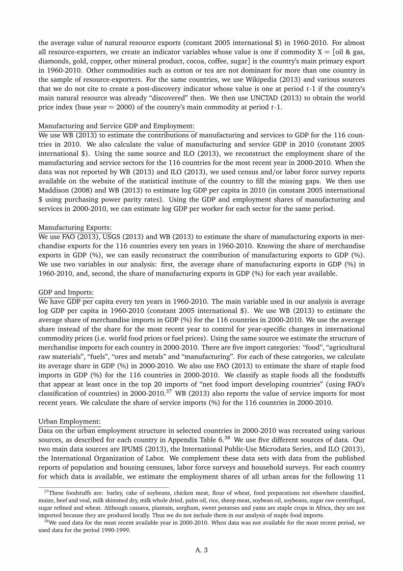
the average value of natural resource exports (constant 2005 international $) in 1960-2010. For almostall resource-exporters, we create an indicator variables whose value is one if commodity X = [oil & gas,diamonds, gold, copper, other mineral product, cocoa, coffee, sugar] is the country’s main primary exportin 1960-2010. Other commodities such as cotton or tea are not dominant for more than one country inthe sample of resource-exporters. For the same countries, we use Wikipedia (2013) and various sourcesthat we do not cite to create a post-discovery indicator whose value is one at period t-1 if the country’smain natural resource was already “discovered” then. We then use UNCTAD (2013) to obtain the worldprice index (base year = 2000) of the country’s main commodity at period t-1.

Manufacturing and Service GDP and Employment:We use WB (2013) to estimate the contributions of manufacturing and services to GDP for the 116 coun-tries in 2010. We also calculate the value of manufacturing and service GDP in 2010 (constant 2005international $). Using the same source and ILO (2013), we reconstruct the employment share of themanufacturing and service sectors for the 116 countries for the most recent year in 2000-2010. When thedata was not reported by WB (2013) and ILO (2013), we used census and/or labor force survey reportsavailable on the website of the statistical institute of the country to fill the missing gaps. We then useMaddison (2008) and WB (2013) to estimate log GDP per capita in 2010 (in constant 2005 international$ using purchasing power parity rates). Using the GDP and employment shares of manufacturing andservices in 2000-2010, we can estimate log GDP per worker for each sector for the same period.

Manufacturing Exports:We use FAO (2013), USGS (2013) and WB (2013) to estimate the share of manufacturing exports in mer-chandise exports for the 116 countries every ten years in 1960-2010. Knowing the share of merchandiseexports in GDP (%), we can easily reconstruct the contribution of manufacturing exports to GDP (%).We use two variables in our analysis: first, the average share of manufacturing exports in GDP (%) in1960-2010, and, second, the share of manufacturing exports in GDP (%) for each year available.

GDP and Imports:We have GDP per capita every ten years in 1960-2010. The main variable used in our analysis is averagelog GDP per capita in 1960-2010 (constant 2005 international $). We use WB (2013) to estimate theaverage share of merchandise imports in GDP (%) for the 116 countries in 2000-2010. We use the averageshare instead of the share for the most recent year to control for year-specific changes in internationalcommodity prices (i.e. world food prices or fuel prices). Using the same source we estimate the structure ofmerchandise imports for each country in 2000-2010. There are five import categories: “food”, “agriculturalraw materials”, “fuels”, “ores and metals” and “manufacturing”. For each of these categories, we calculateits average share in GDP (%) in 2000-2010. We also use FAO (2013) to estimate the share of staple foodimports in GDP (%) for the 116 countries in 2000-2010. We classify as staple foods all the foodstuffsthat appear at least once in the top 20 imports of “net food import developing countries” (using FAO’sclassification of countries) in 2000-2010.37 WB (2013) also reports the value of service imports for mostrecent years. We calculate the share of service imports (%) for the 116 countries in 2000-2010.

Urban Employment:Data on the urban employment structure in selected countries in 2000-2010 was recreated using varioussources, as described for each country in Appendix Table 6.38 We use five different sources of data. Ourtwo main data sources are IPUMS (2013), the International Public-Use Microdata Series, and ILO (2013),the International Organization of Labor. We complement these data sets with data from the publishedreports of population and housing censuses, labor force surveys and household surveys. For each countryfor which data is available, we estimate the employment shares of all urban areas for the following 11

37These foodstuffs are: barley, cake of soybeans, chicken meat, flour of wheat, food preparations not elsewhere classified,maize, beef and veal, milk skimmed dry, milk whole dried, palm oil, rice, sheep meat, soybean oil, soybeans, sugar raw centrifugal,sugar refined and wheat. Although cassava, plantain, sorghum, sweet potatoes and yams are staple crops in Africa, they are notimported because they are produced locally. Thus we do not include them in our analysis of staple food imports.

38We used data for the most recent available year in 2000-2010. When data was not available for the most recent period, weused data for the period 1990-1999.

A. 3

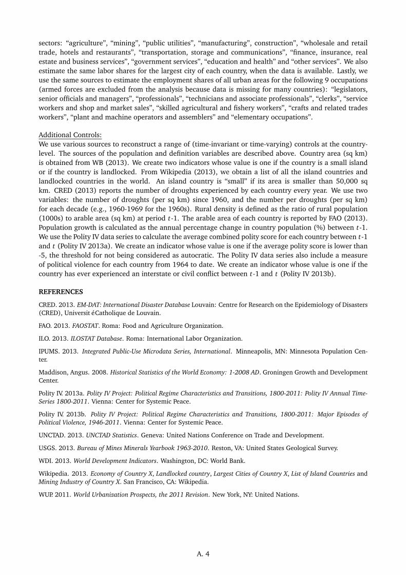
sectors: “agriculture”, “mining”, “public utilities”, “manufacturing”, construction”, “wholesale and retailtrade, hotels and restaurants”, “transportation, storage and communications”, “finance, insurance, realestate and business services”, “government services”, “education and health” and “other services”. We alsoestimate the same labor shares for the largest city of each country, when the data is available. Lastly, weuse the same sources to estimate the employment shares of all urban areas for the following 9 occupations(armed forces are excluded from the analysis because data is missing for many countries): “legislators,senior officials and managers”, “professionals”, “technicians and associate professionals”, “clerks”, “serviceworkers and shop and market sales”, “skilled agricultural and fishery workers”, “crafts and related tradesworkers”, “plant and machine operators and assemblers” and “elementary occupations”.

Additional Controls:We use various sources to reconstruct a range of (time-invariant or time-varying) controls at the country-level. The sources of the population and definition variables are described above. Country area (sq km)is obtained from WB (2013). We create two indicators whose value is one if the country is a small islandor if the country is landlocked. From Wikipedia (2013), we obtain a list of all the island countries andlandlocked countries in the world. An island country is “small” if its area is smaller than 50,000 sqkm. CRED (2013) reports the number of droughts experienced by each country every year. We use twovariables: the number of droughts (per sq km) since 1960, and the number per droughts (per sq km)for each decade (e.g., 1960-1969 for the 1960s). Rural density is defined as the ratio of rural population(1000s) to arable area (sq km) at period t-1. The arable area of each country is reported by FAO (2013).Population growth is calculated as the annual percentage change in country population (%) between t-1.We use the Polity IV data series to calculate the average combined polity score for each country between t-1and t (Polity IV 2013a). We create an indicator whose value is one if the average polity score is lower than-5, the threshold for not being considered as autocratic. The Polity IV data series also include a measureof political violence for each country from 1964 to date. We create an indicator whose value is one if thecountry has ever experienced an interstate or civil conflict between t-1 and t (Polity IV 2013b).

REFERENCES

CRED. 2013. EM-DAT: International Disaster Database Louvain: Centre for Research on the Epidemiology of Disasters(CRED), Université Catholique de Louvain.

FAO. 2013. FAOSTAT. Roma: Food and Agriculture Organization.

ILO. 2013. ILOSTAT Database. Roma: International Labor Organization.

IPUMS. 2013. Integrated Public-Use Microdata Series, International. Minneapolis, MN: Minnesota Population Cen-ter.

Maddison, Angus. 2008. Historical Statistics of the World Economy: 1-2008 AD. Groningen Growth and DevelopmentCenter.

Polity IV. 2013a. Polity IV Project: Political Regime Characteristics and Transitions, 1800-2011: Polity IV Annual Time-Series 1800-2011. Vienna: Center for Systemic Peace.

Polity IV. 2013b. Polity IV Project: Political Regime Characteristics and Transitions, 1800-2011: Major Episodes ofPolitical Violence, 1946-2011. Vienna: Center for Systemic Peace.

UNCTAD. 2013. UNCTAD Statistics. Geneva: United Nations Conference on Trade and Development.

USGS. 2013. Bureau of Mines Minerals Yearbook 1963-2010. Reston, VA: United States Geological Survey.

WDI. 2013. World Development Indicators. Washington, DC: World Bank.

Wikipedia. 2013. Economy of Country X, Landlocked country, Largest Cities of Country X, List of Island Countries andMining Industry of Country X. San Francisco, CA: Wikipedia.

WUP. 2011. World Urbanization Prospects, the 2011 Revision. New York, NY: United Nations.

A. 4

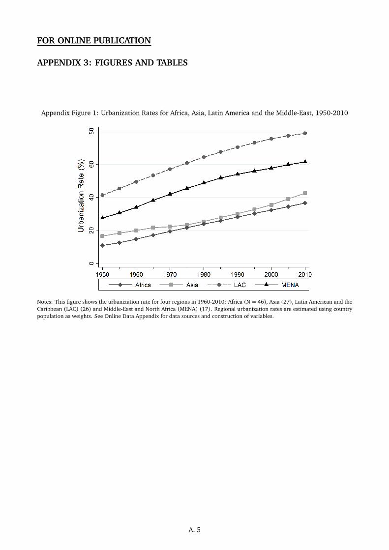
FOR ONLINE PUBLICATION

APPENDIX 3: FIGURES AND TABLES

Appendix Figure 1: Urbanization Rates for Africa, Asia, Latin America and the Middle-East, 1950-2010

Notes: This figure shows the urbanization rate for four regions in 1960-2010: Africa (N = 46), Asia (27), Latin American and theCaribbean (LAC) (26) and Middle-East and North Africa (MENA) (17). Regional urbanization rates are estimated using countrypopulation as weights. See Online Data Appendix for data sources and construction of variables.

A. 5

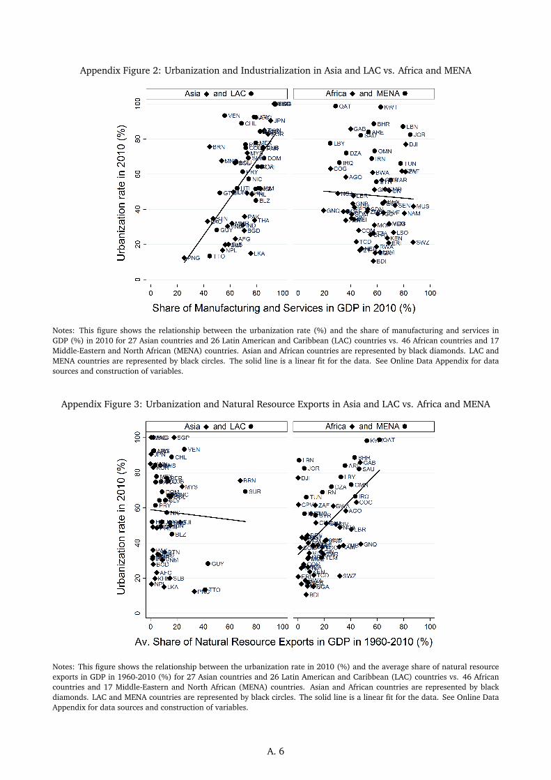
Appendix Figure 2: Urbanization and Industrialization in Asia and LAC vs. Africa and MENA

Notes: This figure shows the relationship between the urbanization rate (%) and the share of manufacturing and services inGDP (%) in 2010 for 27 Asian countries and 26 Latin American and Caribbean (LAC) countries vs. 46 African countries and 17Middle-Eastern and North African (MENA) countries. Asian and African countries are represented by black diamonds. LAC andMENA countries are represented by black circles. The solid line is a linear fit for the data. See Online Data Appendix for datasources and construction of variables.

Appendix Figure 3: Urbanization and Natural Resource Exports in Asia and LAC vs. Africa and MENA

Notes: This figure shows the relationship between the urbanization rate in 2010 (%) and the average share of natural resourceexports in GDP in 1960-2010 (%) for 27 Asian countries and 26 Latin American and Caribbean (LAC) countries vs. 46 Africancountries and 17 Middle-Eastern and North African (MENA) countries. Asian and African countries are represented by blackdiamonds. LAC and MENA countries are represented by black circles. The solid line is a linear fit for the data. See Online DataAppendix for data sources and construction of variables.

A. 6

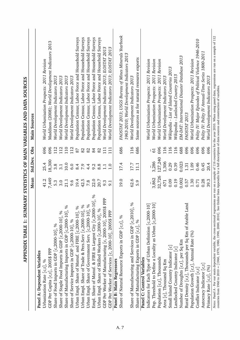
APP

END

IXTA

BLE

1:SU

MM

AR

YST

ATIS

TIC

SO

FM

AIN

VAR

IAB

LES

AN

DD

ATA

SOU

RC

ES

Mea

nSt

d.D

ev.

Obs

Mai

nSo

urc

es

Pan

elA

:D

epen

den

tVa

riab

les

Urb

aniz

atio

nR

ate[c

,t],

%41

.225

.469

6W

orld

Urb

aniz

atio

nPr

ospe

cts:

2011

Revi

sion

GD

PPe

rC

apit

a[c

,t],

2005

$PP

P7,

449

18,3

0069

6M

addi

son

(200

8);W

orld

Dev

elop

men

tIn

dica

tors

2013

Shar

eof

Food

Impo

rts

inG

DP[c

,200

0-10],

%5.

33.

811

2W

orld

Dev

elop

men

tIn

dica

tors

2013

Shar

eof

Stap

leFo

odIm

port

sin

GD

P[c

,200

0-10],

%3.

03.

111

2W

orld

Dev

elop

men

tIn

dica

tors

2013

Shar

eof

Man

ufac

turi

ngIm

port

sin

GD

P[c

,200

0-10],

%21

.110

.011

0W

orld

Dev

elop

men

tIn

dica

tors

2013

Shar

eof

Serv

ice

Impo

rts

inG

DP[c

,200

0-10],

%9.

66.

011

2W

orld

Dev

elop

men

tIn

dica

tors

2013

Urb

anEm

pl.

Shar

eof

Man

uf.

and

FIR

E[c

,200

0-10],

%19

.48.

487

Popu

lati

onC

ensu

s;La

bor

Forc

ean

dH

ouse

hold

Surv

eys

Urb

anEm

pl.

Shar

eof

Trad

e&

Pers

.Ser

v[c

,200

0-10],

%42

.57.

982

Popu

lati

onC

ensu

s;La

bor

Forc

ean

dH

ouse

hold

Surv

eys

Urb

anEm

pl.

Shar

eof

Gov

ernm

ent

Serv

.[c

,200

0-10],

%7.

84.

482

Popu

lati

onC

ensu

s;La

bor

Forc

ean

dH

ouse

hold

Surv

eys

Empl

.Sh

are

ofM

anuf

.&

FIR

Ein

Larg

est

Cit

y[c

,200

0-10],

%22

.09.

284

Popu

lati

onC

ensu

s;La

bor

Forc

ean

dH

ouse

hold

Surv

eys

Urb

anEm

pl.

Shar

eof

Skill

edW

orke

rs[c

,200

0-10],

%20

.78.

882

Popu

lati

onC

ensu

s,La

bor

Forc

ean

dH

ouse

hold

Surv

eys

GD

PPe

rW

orke

rof

Man

ufac

turi

ng[c

,200

0-10],

2005

$PP

P9.

31.

111

1W

orld

Dev

elop

men

tIn

dica

tors

2013

;ILO

STAT

2013

GD

PPe

rW

orke

rof

Serv

ices[c

,200

0-10],

2005

$PP

P9.

11.

011

1W

orld

Dev

elop

men

tIn

dica

tors

2013

;ILO

STAT

2013

Pan

elB

:M

ain

Reg

ress

ors

Shar

eof

Nat

ural

Res

ourc

eEx

port

sin

GD

P[c

,t],

%19

.017

.468

6FA

OST

AT20

13;U

SGS

Bure

auof

Min

esM

iner

als

Year

book

1963

-201

0;W

orld

Dev

elop

men

tIn

dica

tors

2013

Shar

eof

Man

ufac

turi

ngan

dSe

rvic

esin

GD

P[c

,201

0],%

62.6

17.7

116

Wor

ldD

evel

opm

ent

Indi

cato

rs20

13Sh

are

ofM

anuf

actu

ring

Expo

rts

inG

DP[c

,t],

%5.

911

.168

6Sa

me

sour

ces

asfo

rna

tura

lres

ourc

eex

port

sPa

nel

C:

Con

trol

Vari

able

sIn

dica

tors

for

Each

Type

ofU

rban

Defi

niti

on[c

,200

0-10]

__

_W

orld

Urb

aniz

atio

nPr

ospe

cts:

2011

Revi

sion

Pop.

Thre

shol

dto

Defi

nea

Loca

lity

asU

rban[c

,200

0-10]

3,86

23,

286

61W

orld

Urb

aniz

atio

nPr

ospe

cts:

2011

Revi

sion

Popu

lati

on[c

,t],

Thou

sand

s32

,726

127,

240

696

Wor

ldU

rban

izat

ion

Pros

pect

s:20

11Re

visi

onA

rea[c],

Thou

sand

SqK

m67

11,

306

116

Wor

ldD

evel

opm

ent

Indi

cato

rs20

13Sm

allI

slan

dC

ount

ryIn

dica

tor[c]

0.09

0.29

116

Wik

iped

ia-L

ist

ofIs

land

Coun

trie

s20

13La

ndlo

cked

Cou

ntry

Indi

cato

r[c]

0.19

0.39

116

Wik

iped

ia-L

anlo

cked

Coun

try

2013

Num

ber

ofD

roug

hts[c

,t],

per

SqK

m0.

002

0.02

368

8EM

-DAT

:Int

erna

tion

alD

isas

ter

Dat

abas

e20

13R

ural

Den

sity[c

,t],

Thou

sand

spe

rSq

Km

ofA

rabl

eLa

nd0.

571.

3169

6FA

OST

AT20

13Po

pula

tion

Gro

wth[c

,t],

Ann

ualR

ate

(%)

1.30

1.09

696

Wor

ldU

rban

izat

ion

Pros

pect

s:20

11Re

visi

onC

onfli

ctIn

dica

tor[c

,t]

0.71

0.46

696

Polit

yIV

:Maj

orEp

isod

esof

Polit

ical

Viol

ence

1946

-201

0A

utoc

racy

Indi

cato

r[c

,t]

0.28

0.45

696

Polit

yIV

:Pol

ity

IVAn

nual

-Tim

eSe

ries

1800

-201

1Pr

imac

yR

ate[c

,t],

(%)

39.3

20.4

696

Wor

ldD

evel

opm

ent

Indi

cato

rs20

13N

otes

:Pa

nelA

-Fo

rou

rm

ain

depe

nden

tva

riab

le,t

hecr

oss-

sect

iona

lreg

ress

ions

are

run

ona

sam

ple

of11

6co

untr

ies

for

the

year

2010

.W

hen

usin

gpa

neld

ata,

regr

essi

ons

are

run

ona

sam

ple

of11

2co

untr

ies

from

1960

to20

10=[1

960,

1970

,198

0,19

90,2

000,

2010].

See

Onl

ine

Dat

aA

ppen

dix

for

afu

llde

scri

ptio

nof

data

sour

ces

and

cons

truc

tion

ofva

riab

les.

A. 7

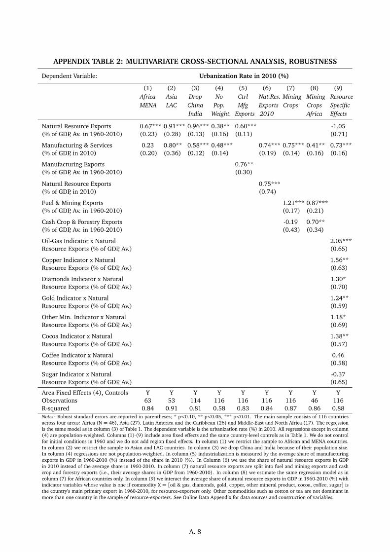
APPENDIX TABLE 2: MULTIVARIATE CROSS-SECTIONAL ANALYSIS, ROBUSTNESS

Dependent Variable: Urbanization Rate in 2010 (%)

(1) (2) (3) (4) (5) (6) (7) (8) (9)Africa Asia Drop No Ctrl Nat.Res. Mining Mining ResourceMENA LAC China Pop. Mfg Exports Crops Crops Specific

India Weight. Exports 2010 Africa Effects

Natural Resource Exports 0.67*** 0.91*** 0.96*** 0.38** 0.60*** -1.05(% of GDP, Av. in 1960-2010) (0.23) (0.28) (0.13) (0.16) (0.11) (0.71)

Manufacturing & Services 0.23 0.80** 0.58*** 0.48*** 0.74*** 0.75*** 0.41** 0.73***(% of GDP, in 2010) (0.20) (0.36) (0.12) (0.14) (0.19) (0.14) (0.16) (0.16)

Manufacturing Exports 0.76**(% of GDP, Av. in 1960-2010) (0.30)

Natural Resource Exports 0.75***(% of GDP, in 2010) (0.74)

Fuel & Mining Exports 1.21*** 0.87***(% of GDP, Av. in 1960-2010) (0.17) (0.21)

Cash Crop & Forestry Exports -0.19 0.70**(% of GDP, Av. in 1960-2010) (0.43) (0.34)

Oil-Gas Indicator x Natural 2.05***Resource Exports (% of GDP, Av.) (0.65)

Copper Indicator x Natural 1.56**Resource Exports (% of GDP, Av.) (0.63)

Diamonds Indicator x Natural 1.30*Resource Exports (% of GDP, Av.) (0.70)

Gold Indicator x Natural 1.24**Resource Exports (% of GDP, Av.) (0.59)

Other Min. Indicator x Natural 1.18*Resource Exports (% of GDP, Av.) (0.69)

Cocoa Indicator x Natural 1.38**Resource Exports (% of GDP, Av.) (0.57)

Coffee Indicator x Natural 0.46Resource Exports (% of GDP, Av.) (0.58)

Sugar Indicator x Natural -0.37Resource Exports (% of GDP, Av.) (0.65)

Area Fixed Effects (4), Controls Y Y Y Y Y Y Y Y YObservations 63 53 114 116 116 116 116 46 116R-squared 0.84 0.91 0.81 0.58 0.83 0.84 0.87 0.86 0.88Notes: Robust standard errors are reported in parentheses; * p<0.10, ** p<0.05, *** p<0.01. The main sample consists of 116 countriesacross four areas: Africa (N = 46), Asia (27), Latin America and the Caribbean (26) and Middle-East and North Africa (17). The regressionis the same model as in column (3) of Table 1. The dependent variable is the urbanization rate (%) in 2010. All regressions except in column(4) are population-weighted. Columns (1)-(9) include area fixed effects and the same country-level controls as in Table 1. We do not controlfor initial conditions in 1960 and we do not add region fixed effects. In column (1) we restrict the sample to African and MENA countries.In column (2) we restrict the sample to Asian and LAC countries. In column (3) we drop China and India because of their population size.In column (4) regressions are not population-weighted. In column (5) industrialization is measured by the average share of manufacturingexports in GDP in 1960-2010 (%) instead of the share in 2010 (%). In Column (6) we use the share of natural resource exports in GDPin 2010 instead of the average share in 1960-2010. In column (7) natural resource exports are split into fuel and mining exports and cashcrop and forestry exports (i.e., their average shares in GDP from 1960-2010). In column (8) we estimate the same regression model as incolumn (7) for African countries only. In column (9) we interact the average share of natural resource exports in GDP in 1960-2010 (%) withindicator variables whose value is one if commodity X = [oil & gas, diamonds, gold, copper, other mineral product, cocoa, coffee, sugar] isthe country’s main primary export in 1960-2010, for resource-exporters only. Other commodities such as cotton or tea are not dominant inmore than one country in the sample of resource-exporters. See Online Data Appendix for data sources and construction of variables.

A. 8

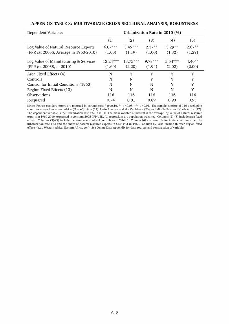
APPENDIX TABLE 3: MULTIVARIATE CROSS-SECTIONAL ANALYSIS, ROBUSTNESS

Dependent Variable: Urbanization Rate in 2010 (%)

(1) (2) (3) (4) (5)

Log Value of Natural Resource Exports 6.07*** 3.45*** 2.37** 3.29** 2.67**(PPP, cst 2005$, Average in 1960-2010) (1.00) (1.19) (1.00) (1.32) (1.29)

Log Value of Manufacturing & Services 12.24*** 13.75*** 9.78*** 5.54*** 4.46**(PPP, cst 2005$, in 2010) (1.60) (2.20) (1.94) (2.02) (2.00)

Area Fixed Effects (4) N Y Y Y YControls N N Y Y YControl for Initial Conditions (1960) N N N Y YRegion Fixed Effects (13) N N N N YObservations 116 116 116 116 116R-squared 0.74 0.81 0.89 0.93 0.95Notes: Robust standard errors are reported in parentheses; * p<0.10, ** p<0.05, *** p<0.01. The sample consists of 116 developingcountries across four areas: Africa (N = 46), Asia (27), Latin America and the Caribbean (26) and Middle-East and North Africa (17).The dependent variable is the urbanization rate (%) in 2010. The main variable of interest is the average log value of natural resourceexports in 1960-2010, expressed in constant 2005 PPP USD. All regressions are population-weighted. Columns (2)-(5) include area fixedeffects. Columns (3)-(5) include the same country-level controls as in Table 1. Column (4) also controls for initial conditions, i.e. theurbanization rate (%) and the share of natural resource exports in GDP (%) in 1960. Column (5) also include thirteen region fixedeffects (e.g., Western Africa, Eastern Africa, etc.). See Online Data Appendix for data sources and construction of variables.

A. 9

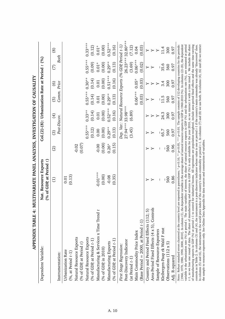
APP

END

IXTA

BLE

4:M

ULT

IVA

RIA

TE

PAN

ELA

NA

LYSI

S,IN

VES

TIG

ATIO

NO

FC

AU

SALI

TY

Dep

ende

ntVa

riab

le:

Nat

.R

esou

rce

Expo

rts

Col

.(2)

-(8)

:U

rban

izat

ion

Rat

eat

Peri

odt

(%)

(%of

GD

P,at

Peri

odt)

(1)

(2)

(3)

(4)

(5)

(6)

(7)

(8)

Inst

rum

enta

tion

:Po

st-D

isco

v.Co

mm

.Pr

ice

Both

Urb

aniz

atio

nR

ate

0.01

(%,a

tPe

riod

t-1)

(0.1

3)N

atur

alR

esou

rce

Expo

rts

-0.0

2(%

ofG

DP,

atPe

riod

t)(0

.07)

Nat

ural

Res

ourc

eEx

port

s0.

55**

*0.

33**

0.55

***

0.30

**0.

55**

*0.

33**

*(%

ofG

DP,

atPe

riod

t-1)

(0.1

2)(0

.14)

(0.1

4)(0

.14)

(0.0

9)(0

.12)

Man

ufac

turi

ng&

Serv

ices

xTi

me

Tren

dt

-0.0

1***

-0.0

00.

000.

010.

010.

010.

01*

0.01

*(%

ofG

DP,

in20

10)

(0.0

0)(0

.00)

(0.0

0)(0

.00)

(0.0

0)(0

.00)

(0.0

0)(0

.00)

Man

ufac

turi

ngEx

port

s-0

.08

0.26

*0.

29**

0.52

***

0.29

**0.

51**

*0.

29**

0.52

***

(%of

GD

P,at

Peri

odt-

1)(0

.35)

(0.1

5)(0

.13)

(0.1

6)(0

.13)

(0.1

6)(0

.13)

(0.1

6)

Firs

tSt

age

Regr

essi

on:

Dep

.Va

r.:N

atur

alRe

sour

ceEx

port

s(%

GD

P,Pe

riod

t-1)

Post

-Dis

cove

ryIn

dica

tor

27.9

4***

33.9

8***

26.2

3***

32.8

0***

(at

Peri

odt-

1)(3

.45)

(6.8

9)(3

.69)

(7.1

2)M

ain

Com

mod

ity

Pric

eIn

dex

0.06

***

0.05

*0.

06**

*0.

04(B

ase

Peri

od=

2000

,at

Peri

odt-

1)(0

.03)

(0.0

3)(0

.02)

(0.0

3)C

ount

ryan

dPe

riod

Fixe

dEf

fect

s(1

12;5

)Y

YY

YY

YY

YA

rea-

Peri

odFi

xed

Effe

cts

(4x

5),C

ontr

ols

YY

YY

YY

YY

Sam

ple

ofR

esou

rce-

Expo

rter

s_

__

Y_

Y_

YK

leib

erge

n-Pa

aprk

Wal

dF

stat

__

65.7

24.3

11.5

3.4

35.6

11.4

Obs

erva

tion

s(1

12x

5)56

056

056

030

056

030

056

030

0A

dj.

R-s

quar

ed0.

860.

960.

970.

970.

970.

970.

970.

97N

otes

:R

obus

tsta

ndar

der

rors

clus

tere

dat

the

coun

try

leve

lare

repo

rted

inpa

rent

hese

s;*

p<0.

10,*

*p<

0.05

,***

p<0.

01.

The

sam

ple

cons

ists

of11

2de

velo

ping

coun

trie

sfo

rth

epe

riod

s:[1

960,

1970

,198

0,19

90,2

000,

2010].

Inco

lum

n(1

),th

ede

pend

entv

aria

ble

isth

eav

erag

esh

are

ofna

tura

lres

ourc

eex

port

sin

GD

Pin

1960

-201

0(%

).In

colu

mns

(2)-

(8),

the

depe

nden

tva

riab

leis

the

urba

niza

tion

rate

(%)

atpe

riod

t.Th

em

ain

vari

able

sof

inte

rest

,the

shar

eof

natu

ralr

esou

rce

expo

rts

inG

DP

(%)

and

the

urba

niza

tion

rate

(%),

are

esti

mat

edat

peri

odt-

1,so

we

lose

one

roun

dof

data

.Th

esh

are

ofm

anuf

actu

ring

and

serv

ices

inG

DP

(%)

ison

lyav

aila

ble

for

the

year

2010

,so

we

inte

ract

itw

ith

ati

me

tren

dt.

We

incl

ude

the

shar

eof

man

ufac

turi

ngex

port

sin

GD

P(%

)at

peri

odt-

1to

cont

rol

for

indu

stri

albo

oms.

All

regr

essi

ons

are

popu

lati

on-w

eigh

ted,

incl

ude

area

-per

iod

fixed

effe

cts

and

the

sam

eti

me-

vary

ing

cont

rols

asin

Tabl

e2.

Inco

lum

ns(3

)an

d(4

),th

ein

stru

men

tis

apo

st-d

isco

very

indi

cato

rw

hose

valu

eis

one

atpe

riod

t-1

ifth

eco

untr

y’s

mai

nco

mm

odit

yw

asal

read

y“d

isco

vere

d”th

en.

Inco

lum

ns(5

)an

d(6

),th

ein

stru

men

tis

the

wor

ldpr

ice

inde

xof

the

coun

try’

sm

ain

com

mod

ity

atpe

riod

t-1.

Inco

lum

ns(7

)an

d(8

)w

eus

ebo

th.

Inco

lum

ns(4

),(6

)an

d(8

)w

ere

stri

ctth

esa

mpl

eto

reso

urce

-exp

orte

rson

ly.

See

Onl

ine

Dat

aA

ppen

dix

for

data

sour

ces

and

cons

truc

tion

ofva

riab

les.

A. 10

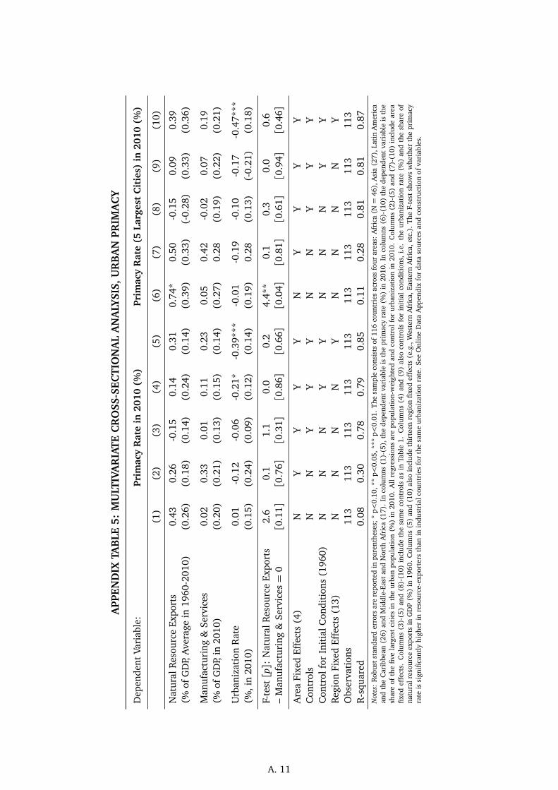
APP

END

IXTA

BLE

5:M

ULT

IVA

RIA

TE

CR

OSS

-SEC

TIO

NA

LA

NA

LYSI

S,U

RB

AN

PRIM

AC

Y

Dep

ende

ntVa

riab

le:

Prim

acy

Rat

ein

2010

(%)

Prim

acy

Rat

e(5

Larg

est

Cit

ies)

in20

10(%

)

(1)

(2)

(3)

(4)

(5)

(6)

(7)

(8)

(9)

(10)

Nat

ural

Res

ourc

eEx

port

s0.

430.

26-0

.15

0.14

0.31

0.74

*0.

50-0

.15

0.09

0.39

(%of

GD

P,A

vera

gein

1960

-201

0)(0

.26)

(0.1

8)(0

.14)

(0.2

4)(0

.14)

(0.3

9)(0

.33)

(-0.

28)

(0.3

3)(0

.36)

Man

ufac

turi

ng&

Serv

ices

0.02

0.33

0.01

0.11

0.23

0.05

0.42

-0.0

20.

070.

19(%

ofG

DP,

in20

10)

(0.2

0)(0

.21)

(0.1

3)(0

.15)

(0.1

4)(0

.27)

0.28

(0.1

9)(0

.22)

(0.2

1)

Urb

aniz

atio

nR

ate

0.01

-0.1

2-0

.06

-0.2

1*-0

.39*

**-0

.01

-0.1

9-0

.10

-0.1

7-0

.47*

**(%

,in

2010

)(0

.15)

(0.2

4)(0

.09)

(0.1

2)(0

.14)

(0.1

9)0.

28(0

.13)

(-0.

21)

(0.1

8)

F-te

st[p]:

Nat

ural

Res

ourc

eEx

port

s2.

60.

11.

10.

00.

24.

4**

0.1

0.3

0.0

0.6

–M

anuf

actu

ring

&Se

rvic

es=

0[0

.11]

[0.7

6][0

.31]

[0.8

6][0

.66]

[0.0

4][0

.81]

[0.6

1][0

.94]

[0.4

6]

Are

aFi

xed

Effe

cts

(4)

NY

YY

YN

YY

YY

Con

trol

sN

NY

YY

NN

YY

YC

ontr

olfo

rIn

itia

lCon

diti

ons

(196

0)N

NN

YY

NN

NY

YR

egio

nFi

xed

Effe

cts

(13)

NN

NN

YN

NN

NY

Obs

erva

tion

s11

311

311

311

311

311

311

311

311

311

3R

-squ

ared

0.08

0.30

0.78

0.79

0.85

0.11

0.28

0.81

0.81

0.87

Not

es:

Rob

ust

stan

dard

erro

rsar

ere

port

edin

pare

nthe

ses;

*p<

0.10

,**

p<0.

05,*

**p<

0.01

.Th

esa

mpl

eco

nsis

tsof

116

coun

trie

sac

ross

four

area

s:A

fric

a(N=

46),

Asi

a(2

7),L

atin

Am

eric

aan

dth

eC

arib

bean

(26)

and

Mid

dle-

East

and

Nor

thA

fric

a(1

7).

Inco

lum

ns(1

)-(5

),th

ede

pend

ent

vari

able

isth

epr

imac

yra

te(%

)in

2010

.In

colu

mns

(6)-

(10)

the

depe

nden

tva

riab

leis

the

shar

eof

the

five

larg

est

citi

esin

the

urba

npo

pula

tion

(%)

in20

10.

All

regr

essi

ons

are

popu

lati

on-w

eigh

ted

and

cont

rolf

orur

bani

zati

onin

2010

.C

olum

ns(2

)-(5

)an

d(7

)-(1

0)in

clud

ear

eafix

edef

fect

s.C

olum

ns(3

)-(5

)an

d(8

)-(1

0)in

clud

eth

esa

me

cont

rols

asin

Tabl

e1.

Col

umns

(4)

and

(9)

also

cont

rols

for

init

ial

cond

itio

ns,

i.e.

the

urba

niza

tion

rate

(%)

and

the

shar

eof

natu

ralr

esou

rce

expo

rts

inG

DP

(%)

in19

60.

Col

umns

(5)

and

(10)

also

incl

ude

thir

teen

regi

onfix

edef

fect

s(e

.g.,

Wes

tern

Afr

ica,

East

ern

Afr

ica,

etc.

).Th

eF-

test

show

sw

heth

erth

epr

imac

yra

teis

sign

ifica

ntly

high

erin

reso

urce

-exp

orte

rsth

anin

indu

stri

alco

untr

ies

for

the

sam

eur

bani

zati

onra

te.

See

Onl

ine

Dat

aA

ppen

dix

for

data

sour

ces

and

cons

truc

tion

ofva

riab

les.

A. 11

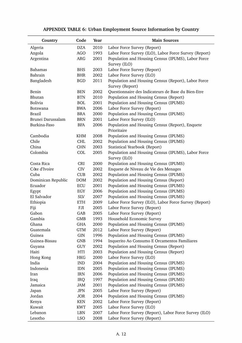
APPENDIX TABLE 6: Urban Employment Source Information by Country

Country Code Year Main Sources

Algeria DZA 2010 Labor Force Survey (Report)Angola AGO 1993 Labor Force Survey (ILO), Labor Force Survey (Report)Argentina ARG 2001 Population and Housing Census (IPUMS), Labor Force

Survey (ILO)Bahamas BHS 2003 Labor Force Survey (Report)Bahrain BHR 2002 Labor Force Survey (ILO)Bangladesh BGD 2011 Population and Housing Census (Report), Labor Force

Survey (Report)Benin BEN 2002 Questionnaire des Indicateurs de Base du Bien-EtreBhutan BTN 2010 Population and Housing Census (Report)Bolivia BOL 2001 Population and Housing Census (IPUMS)Botswana BWA 2006 Labor Force Survey (Report)Brazil BRA 2000 Population and Housing Census (IPUMS)Brunei Darussalam BRN 2001 Labor Force Survey (ILO)Burkina-Faso BFA 2006 Population and Housing Census (Report), Enquete

PrioritaireCambodia KHM 2008 Population and Housing Census (IPUMS)Chile CHL 2002 Population and Housing Census (IPUMS)China CHN 2003 Statistical Yearbook (Report)Colombia COL 2005 Population and Housing Census (IPUMS), Labor Force

Survey (ILO)Costa Rica CRI 2000 Population and Housing Census (IPUMS)Côte d’Ivoire CIV 2002 Enquete de Niveau de Vie des MenagesCuba CUB 2002 Population and Housing Census (IPUMS)Dominican Republic DOM 2002 Population and Housing Census (Report)Ecuador ECU 2001 Population and Housing Census (IPUMS)Egypt EGY 2006 Population and Housing Census (IPUMS)El Salvador SLV 2007 Population and Housing Census (IPUMS)Ethiopia ETH 2009 Labor Force Survey (ILO), Labor Force Survey (Report)Fiji FJI 2005 Labor Force Survey (Report)Gabon GAB 2005 Labor Force Survey (Report)Gambia GMB 1993 Household Economic SurveyGhana GHA 2000 Population and Housing Census (IPUMS)Guatemala GTM 2012 Labor Force Survey (Report)Guinea GIN 1996 Population and Housing Census (IPUMS)Guinea-Bissau GNB 1994 Inquerito Ao Consumo E Orcamentos FamiliaresGuyana GUY 2002 Population and Housing Census (Report)Haiti HTI 2003 Population and Housing Census (Report)Hong Kong HKG 2000 Labor Force Survey (ILO)India IND 2004 Population and Housing Census (IPUMS)Indonesia IDN 2005 Population and Housing Census (IPUMS)Iran IRN 2006 Population and Housing Census (IPUMS)Iraq IRQ 1997 Population and Housing Census (IPUMS)Jamaica JAM 2001 Population and Housing Census (IPUMS)Japan JPN 2005 Labor Force Survey (Report)Jordan JOR 2004 Population and Housing Census (IPUMS)Kenya KEN 2002 Labor Force Survey (Report)Kuwait KWT 2005 Labor Force Survey (ILO)Lebanon LBN 2007 Labor Force Survey (Report), Labor Force Survey (ILO)Lesotho LSO 2008 Labor Force Survey (Report)

A. 12

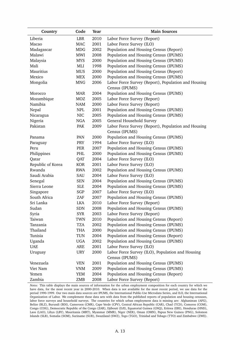
Country Code Year Main Sources

Liberia LBR 2010 Labor Force Survey (Report)Macao MAC 2001 Labor Force Survey (ILO)Madagascar MDG 2002 Population and Housing Census (Report)Malawi MWI 2008 Population and Housing Census (IPUMS)Malaysia MYS 2000 Population and Housing Census (IPUMS)Mali MLI 1998 Population and Housing Census (IPUMS)Mauritius MUS 2000 Population and Housing Census (Report)Mexico MEX 2000 Population and Housing Census (IPUMS)Mongolia MNG 2006 Labor Force Survey (Report), Population and Housing

Census (IPUMS)Morocco MAR 2004 Population and Housing Census (IPUMS)Mozambique MOZ 2005 Labor Force Survey (Report)Namibia NAM 2000 Labor Force Survey (Report)Nepal NPL 2001 Population and Housing Census (IPUMS)Nicaragua NIC 2005 Population and Housing Census (IPUMS)Nigeria NGA 2005 General Household SurveyPakistan PAK 2009 Labor Force Survey (Report), Population and Housing

Census (IPUMS)Panama PAN 2000 Population and Housing Census (IPUMS)Paraguay PRY 1994 Labor Force Survey (ILO)Peru PER 2007 Population and Housing Census (IPUMS)Philippines PHL 2000 Population and Housing Census (IPUMS)Qatar QAT 2004 Labor Force Survey (ILO)Republic of Korea KOR 2001 Labor Force Survey (ILO)Rwanda RWA 2002 Population and Housing Census (IPUMS)Saudi Arabia SAU 2004 Labor Force Survey (ILO)Senegal SEN 2004 Population and Housing Census (IPUMS)Sierra Leone SLE 2004 Population and Housing Census (IPUMS)Singapore SGP 2007 Labor Force Survey (ILO)South Africa ZAF 2007 Population and Housing Census (IPUMS)Sri Lanka LKA 2010 Labor Force Survey (Report)Sudan SDN 2008 Population and Housing Census (IPUMS)Syria SYR 2003 Labor Force Survey (Report)Taiwan TWN 2010 Population and Housing Census (Report)Tanzania TZA 2002 Population and Housing Census (IPUMS)Thailand THA 2000 Population and Housing Census (IPUMS)Tunisia TUN 2004 Population and Housing Census (Report)Uganda UGA 2002 Population and Housing Census (IPUMS)UAE ARE 2001 Labor Force Survey (ILO)Uruguay URY 2000 Labor Force Survey (ILO), Population and Housing

Census (IPUMS)Venezuela VEN 2001 Population and Housing Census (IPUMS)Viet Nam VNM 2009 Population and Housing Census (IPUMS)Yemen YEM 2004 Population and Housing Census (Report)Zambia ZMB 2008 Labor Force Survey (Report)Notes: This table displays the main sources of information for the urban employment composition for each country for which wehave data, for the most recent year in 2000-2010. When data is not available for the most recent period, we use data for theperiod 1990-1999. Our two main data sources are IPUMS, the International Public-Use Microdata Series, and ILO, the InternationalOrganization of Labor. We complement these data sets with data from the published reports of population and housing censuses,labor force surveys and household surveys. The countries for which urban employment data is missing are: Afghanistan (AFG),Belize (BLZ), Burundi (BDI), Cameroon (CMR), Cape Verde (CPV), Central African Republic (CAR), Chad (TCD), Comoros (COM),Congo (COG), Democratic Republic of the Congo (ZAR), Djibouti (DJI), Equatorial Guinea (GNQ), Eritrea (ERI), Honduras (HND),Laos (LAO), Libya (LBY), Mauritania (MRT), Myanmar (MMR), Niger (NER), Oman (OMN), Papua New Guinea (PNG), SolomonIslands (SLB), Somalia (SOM), Suriname (SUR), Swaziland (SWZ), Togo (TGO), Trinidad and Tobago (TTO) and Zimbabwe (ZWE).

A. 13