Embed Size (px)
Citation preview

Urban Stormwater Treatment by Experimental Constructed Wetlands
Swarthmore College Department of Engineering
Colton Bangs May 16, 2007
Engineering 90
Senior Design Project
Advisor: Professor Arthur E. McGarity

Abstract
The conclusion of my studies in the Swarthmore College Engineering Department
was the engineering design project for improving an existing constructed wetland built as
an experiment for treating stormwater. My project entailed four main areas: hydrologic
modeling, improving the wetland flow and level control system, designing a solar energy
system for powering the wetland operation and monitoring, and assessing the
performance of the system. The final results for system performance indicate that
wetland plants are instrumental in nutrient removal. The planted channel of the wetland
saw concentration removal efficiencies for nitrate and phosphate at 26% and 59%,
respectively. The unplanted channel had no significant nutrient removal. Gathering help
from fellow engineering students and guidance from several of the engineering faculty,
this project began with some preliminary work in the fall of 2006 and culminated in this
report and a presentation in May, 2007. The wetland system is now in place for
educational use by the Engineering Department and plans are drawn out for the future of
the project.
2

URBAN STORMWATER TREATMENT BY EXPERIMENTAL CONSTRUCTED WETLANDS 1
ABSTRACT 2
1. INTRODUCTION 5
STORMWATER MANAGEMENT 5 SITE HISTORY 7 MARC JEULAND, E90, SPRING 2001 9 WATER QUALITY AND POLLUTION CONTROL, E63, FALL 2006 10 PROJECT OVERVIEW 11
2. HYDROLOGIC MODELING 12
GEOGRAPHIC INFORMATION SYSTEMS (GIS) 13 STORM MONITORING 19 LINEAR PROGRAMMING 22 HEC-HMS 24
3. FLOW AND LEVEL CONTROL 26
INFLOW GATE 27 FLOWMETER 28 PULSE COUNTER 30 FLOW CONTROL 31 OUTFLOW GATE 32
4. SOLAR ENERGY SYSTEM 35
SIZING 36 ELECTRICAL LOAD DETERMINATION 36 BATTERY STORAGE 37 PHOTOVOLTAIC (PV) PANELS 38 SOLAR ARRAY 38 SOLAR PATHFINDER 39 BASIC ARRAY DESIGN 41
5. SYSTEM PERFORMANCE 43
LATEST RESULTS 44 MEASUREMENT CONTINUITY AND CALIBRATION 44 TRANSIENT STATE 46 NUTRIENT REMOVAL OVER CHANNEL LENGTH 48 MARC JEULAND, 2001 52 E63, FALL 2006 54
3

6. CONCLUSION AND FUTURE WORK 57
REALISTIC DESIGN CONSTRAINTS 57 ECONOMIC 58 ENVIRONMENTAL 58 SUSTAINABILITY 58 MANUFACTURABILITY 59 ETHICAL 59 HEALTH AND SAFETY 59 COST SUMMARY 59 FUTURE WORK 60 HYDROLOGIC MODELING 60 FLOW AND LEVEL CONTROL 60 SOLAR ENERGY SYSTEM 60 WETLAND PERFORMANCE 60 ACKNOWLEDGEMENTS 61 APPENDIX 61
4

1. Introduction
Stormwater Management
In 1972, under growing public awareness of the impacts of water pollution, the
Clean Water Act was passed by the U.S. Federal Government to control pollution in the
nation’s surface waters. This began by regulating point source polluters in industry and
funding the construction of wastewater treatment plants to clean up sewage before being
discharged to the environment. Regulation of point source water pollution was part of
the Clean Water Act Phase I. In the late 1980’s, efforts began to plan for implementation
of Phase II to address nonpoint water pollution from stormwater runoff. Only recently
has Phase II come into action, with municipalities being required to have permits for their
storm sewer systems. The initial requirement of municipalities is simply to map their
current storm sewer systems. In the future, there will be increased demands by the EPA
and state DEPs which is why we need to act now to cleanup stormwater runoff. An
overall view of the Clean Water Act is shown in Figure 1-1.
5

Figure 1-1 Overview of the Clean Water Act and its regulatory process1.
The EPA has identified the lower Crum Creek, which drains all of Swarthmore College
as an impaired water body and placed it in on the 303(d) list. Eventually, total-maximum
daily loads (TMDLs) will be developed for the lower Crum and point and nonpoint
pollution strategies will have to be developed to improve the water quality to a
satisfactory level.
Swarthmore College is currently practicing responsible stormwater management
under the regulation of the Swarthmore Borough. The borough requires that all new
construction and renovations increasing impervious area by 400 square feet or more have
a drainage plan for stormwater management.2 Swarthmore College facilities, as a
practice, are trying to stay ahead of the curve by exceeding borough regulations where
possible. The college has done this through the use of green roofs, recharge basins,
biostreams and cisterns. The newest dorm on campus, Alice Paul, is equipped with a
green roof which absorbs some precipitation as well as cuts down on heating and air 1 U.S. EPA, http://www.epa.gov/watertrain/cwa/cwa1.htm 2 Swarthmore Borough, http://www.swarthmorepa.org/government/permits.asp
6

conditioning costs. Alice Paul and the three dorm complex PPR have recharge basins
designed to hold back rainfall from a 2-year storm event and recharge the water to the
groundwater. A biostream was constructed behind the McCabe Library to collect
stormwater from it and surrounding buildings. It slows the water down on its way to its
discharge into Crum Creek and helps to remove some of the pollutants. There are several
underground cisterns located on campus which are used to collect stormwater. Under the
Science Center lawn, a 35,000 gallon cistern captures water from the building to use later
for irrigation. An even larger cistern of 100,000 gallons is located under the drive
between Martin and Lang Music Hall and is designed to collect heavy rains from summer
thunderstorms and discharge the stormwater slowly into the Crum to prevent erosion.
Another potential candidate for stormwater management at Swarthmore College is a
constructed wetland for retaining and treating runoff.
Site History
The wetland is located in the Crum Woods alongside a first order open stream
channel, known as C40. C40 transports water from a storm sewer outfall behind the
Mullan Tennis Center to the Crum Creek. This stream runs roughly 150 meters as an
open channel before reaching the 303(d) listed lower reach of the Crum Creek. The
outfall behind the Mullan Center is known by the Swarthmore Environmental Lab
terminology as C40A and drains a large portion of the college campus as well as Chester
Road (Route 320) and the SEPTA train station. Figure 1-2 shows a map of the area under
discussion here.
7

Figure 1-2. Map of the area around the wetland. The yellow star indicates the outfall from C40A, the red star is the location of the wetland, and the blue star is upstream of the point of discharge of the C40 stream (light blue).
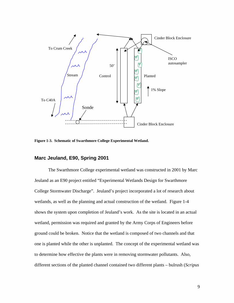
Figure 1-3 shows a schematic of the wetland from above. Water enters an
underground pipe where its quality is measured by the Sonde. When it reaches the inflow
cinder block enclosure, it is pumped up to the height of the wetland and distributed to the
two channels. The water flows through the wetland down a 1% slope and is sampled by
the ISCO autosampler just before it clears the outflow gate. This water is then returned
to the stream and eventually it enters the Crum Creek.
8
Stream
To C40A
To Crum Creek
Cinder Block Enclosure
Cinder Block Enclosure
Sonde
Planted Control
50’
ISCO autosampler
1% Slope
Figure 1-3. Schematic of Swarthmore College Experimental Wetland.
Marc Jeuland, E90, Spring 2001
The Swarthmore College experimental wetland was constructed in 2001 by Marc
Jeuland as an E90 project entitled “Experimental Wetlands Design for Swarthmore
College Stormwater Discharge”. Jeuland’s project incorporated a lot of research about
wetlands, as well as the planning and actual construction of the wetland. Figure 1-4
shows the system upon completion of Jeuland’s work. As the site is located in an actual
wetland, permission was required and granted by the Army Corps of Engineers before
ground could be broken. Notice that the wetland is composed of two channels and that
one is planted while the other is unplanted. The concept of the experimental wetland was
to determine how effective the plants were in removing stormwater pollutants. Also,
different sections of the planted channel contained two different plants – bulrush (Scripus
9

pungens) and burreed (Sparganium americanum). The channels were fed from C40
upstream, through a gravity-powered system that consisted of two hoses and a screen.
The system was prone to clogging and turned out to be infeasible for the project.
Figure 1-4. The wetland as constructed by Marc Jeuland '01.
Jeuland was only able to do some preliminary testing of pollutant removal efficiencies
before the project ended. He remarks that his data is not to be trusted because it was
taken too soon after planting.
Water Quality and Pollution Control, E63, Fall 2006
Five years later, the project was brought back to life by the hard work of a group of
E63 students led by Professor Arthur McGarity. Fellow Engineering student Perry
Carlson ‘08 and I began the site recovery with an archaeological-like expedition to
10

remove the overgrowth and reopen the site. The class helped to replant bulrush into the
experimental (planted) channel, while, as per Jeuland’s design, the other channel was left
as a control. The significant problem with Jeuland’s design, the gravity-fed inflow
system, was overhauled and replaced with two garden fountain pumps running off battery
power. This system proved to be successful, though with the inconvenience and
downtime of having to return the heavy marine batteries to the lab for charging. Two
cinder-block enclosures, one at the top of the wetland and one at the bottom, were
installed to protect equipment from weather and vandals. The main accomplishment of
the class was to get the system set up and running functionally. Beyond that, there was
some monitoring of system performance and storm events, as well as an attempt to
measure the hydraulic retention time with both salt and dye. A final report was produced
describing the work of the class on the wetland.
Project Overview
The project that I took up was to improve upon the work of those past-involved with
the wetland. These improvements can be categorized into four sections:
1) Hydrologic Modeling
2) Flow and Level Control
3) Solar Electric System
4) Wetland Performance
The rationale behind each is as follows: Hydrological modeling was sought to
characterize the flows from C40A to better inform wetland use. A system for flow and
level control was needed to calculate and control pollutant loadings on the wetland and
control the water level in the wetland. A solar electric system was wanted to supply
11

power for the instruments needed for monitoring and operation of the site so that it could
be self-powered. Finally, more data regarding the performance of the wetland was
sought to add to and compare with the small database of current performance data. The
report from here on is divided into these sections with a conclusion at the end to
recommend future progress at the wetland.
2. Hydrologic Modeling Hydrological modeling in this project incorporated basic hydrologic theory, GIS,
HEC-HMS and actual storm data. GIS mapping was used to map the watershed drained
by C40A and extract parameters from it such as area and land use. HEC-HMS is a
hydrologic computer modeling program developed by the Army Corps of Engineers and
was used to model the C40A outflow based on GIS parameters and storm data. The
ISCO 6712 autosampler was employed at C40A to monitor several spring storms and
provide data for building and authenticating the model. The concept map in Figure 2-1
gives an idea of the process I undertook in constructing a hydrologic model.
12
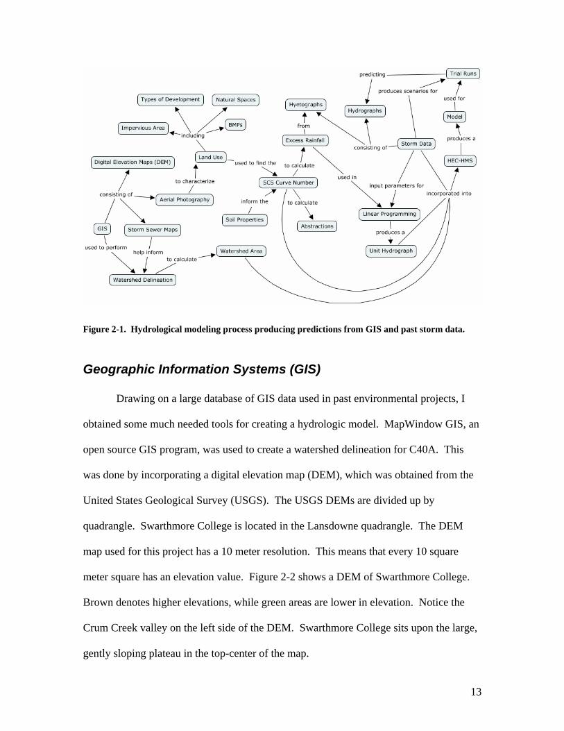
Figure 2-1. Hydrological modeling process producing predictions from GIS and past storm data.
Geographic Information Systems (GIS) Drawing on a large database of GIS data used in past environmental projects, I
obtained some much needed tools for creating a hydrologic model. MapWindow GIS, an
open source GIS program, was used to create a watershed delineation for C40A. This
was done by incorporating a digital elevation map (DEM), which was obtained from the
United States Geological Survey (USGS). The USGS DEMs are divided up by
quadrangle. Swarthmore College is located in the Lansdowne quadrangle. The DEM
map used for this project has a 10 meter resolution. This means that every 10 square
meter square has an elevation value. Figure 2-2 shows a DEM of Swarthmore College.
Brown denotes higher elevations, while green areas are lower in elevation. Notice the
Crum Creek valley on the left side of the DEM. Swarthmore College sits upon the large,
gently sloping plateau in the top-center of the map.
13

Figure 2-2. Swarthmore College digital elevation map (DEM).
Typical watershed delineations can be done on DEMs, however, MapWindow
allows the user to insert shapefiles to denote the existence of streams. This feature allows
the user to create conditions that are more realistic if the locations of storm sewers and
streams are known. Figure 2-3 shows an aerial photography map of the college with a
customized shape file that I have created to account for the location of streams and storm
sewers. Note that in several cases, streets actually double as storm sewers – such as
Chester Road.
14
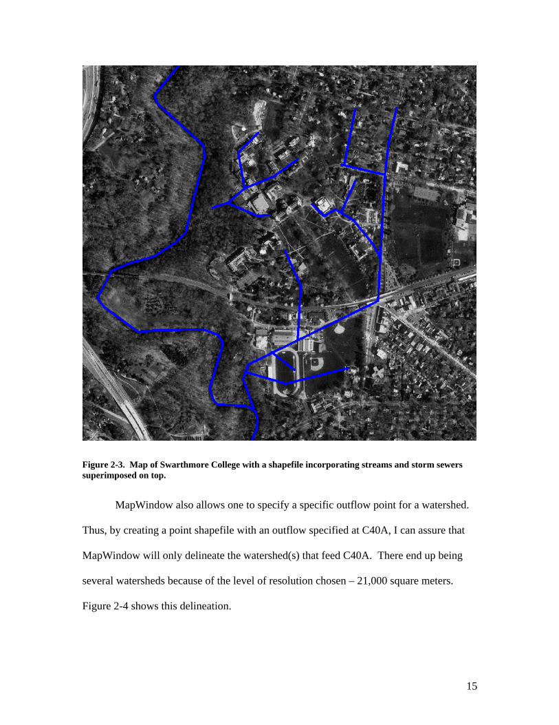
Figure 2-3. Map of Swarthmore College with a shapefile incorporating streams and storm sewers superimposed on top.
MapWindow also allows one to specify a specific outflow point for a watershed.
Thus, by creating a point shapefile with an outflow specified at C40A, I can assure that
MapWindow will only delineate the watershed(s) that feed C40A. There end up being
several watersheds because of the level of resolution chosen – 21,000 square meters.
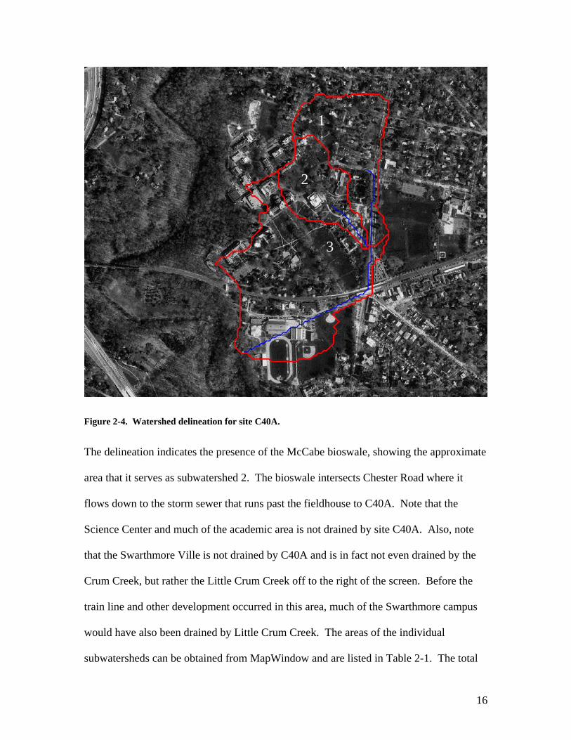
Figure 2-4 shows this delineation.
15
1
2
3
Figure 2-4. Watershed delineation for site C40A.
The delineation indicates the presence of the McCabe bioswale, showing the approximate
area that it serves as subwatershed 2. The bioswale intersects Chester Road where it
flows down to the storm sewer that runs past the fieldhouse to C40A. Note that the
Science Center and much of the academic area is not drained by site C40A. Also, note
that the Swarthmore Ville is not drained by C40A and is in fact not even drained by the
Crum Creek, but rather the Little Crum Creek off to the right of the screen. Before the
train line and other development occurred in this area, much of the Swarthmore campus
would have also been drained by Little Crum Creek. The areas of the individual
subwatersheds can be obtained from MapWindow and are listed in Table 2-1. The total
16

watershed area that drains C40A was found to be 384,125 square meters or about 95
acres.
Subwatershed Area (sq. meters)
1 96,375
2 64,362.5
3 223,387.5
Total 384,125
Table 2-1. Watershed areas for C40A.
Now that we have the watershed area, the land use characterizations are the next
parameters to extract from the GIS data. I began by creating a shapefile to roughly
indicate known impervious surfaces. This included large buildings, parking lots and
roads. The impervious surface shapefile is shown in Figure 2-5. This process was also
done for large open areas, which can be seen in Appendix 1. The open areas were
assumed to be in good condition, which means that they have more than 75% grass
coverage. The rest of the watershed is considered to be residential with ½ acre lots on
average. Table 2-2 shows the breakdown of all land use categorizations. Residential
land use leads the way at about 53%, with impervious surfaces at 24.49% and open areas
at 22.51%.
17
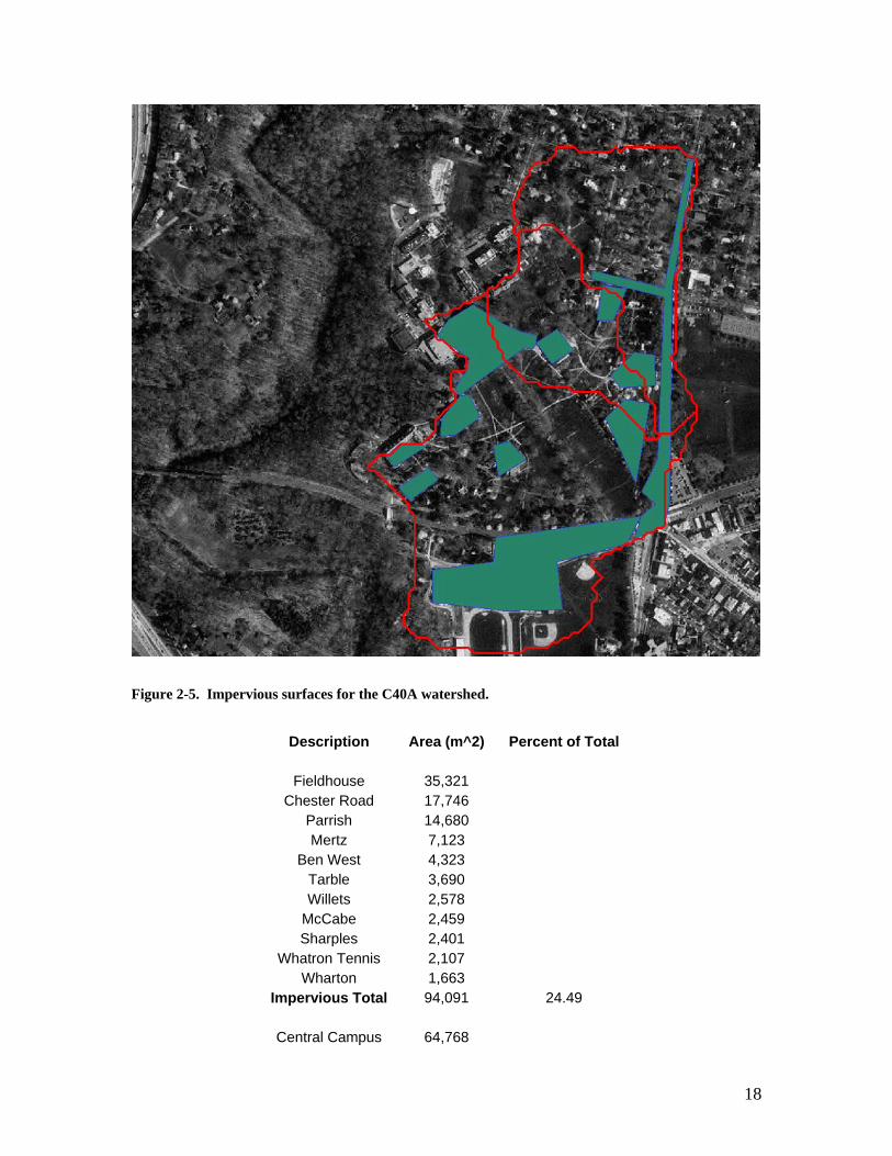
Figure 2-5. Impervious surfaces for the C40A watershed.
Description Area (m^2) Percent of Total
Fieldhouse 35,321
Chester Road 17,746 Parrish 14,680 Mertz 7,123
Ben West 4,323 Tarble 3,690 Willets 2,578
McCabe 2,459 Sharples 2,401
Whatron Tennis 2,107 Wharton 1,663
Impervious Total 94,091 24.49
Central Campus 64,768
18
Baseball Field 10,948 Rose Garden 10,765
Open Area Total 86,481 22.51
Residential Total 203,553 52.99
Overall Total 384,125 100.00
Table 2-2. Land use breakdown by type and area.
Using this land use data, I calculated the SCS Curve Number for the watershed
assuming Hydrologic Soil Group C – clay, shallow sandy loam. I used an area-weighted
average of the values for the three land uses – Open Area, Impervious Surface, and
Residential. These values for group C are 74, 98, and 80, respectively. Thus, I obtained
a value of 83 for the SCS Curve Number. This number will be used to model the
abstractions (losses) of stormwater to groundwater flow. To reiterate, from the GIS
modeling I obtained the watershed area and SCS Curve Number.
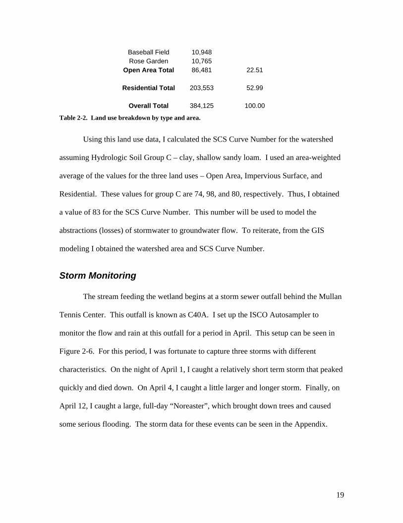
Storm Monitoring The stream feeding the wetland begins at a storm sewer outfall behind the Mullan
Tennis Center. This outfall is known as C40A. I set up the ISCO Autosampler to
monitor the flow and rain at this outfall for a period in April. This setup can be seen in
Figure 2-6. For this period, I was fortunate to capture three storms with different
characteristics. On the night of April 1, I caught a relatively short term storm that peaked
quickly and died down. On April 4, I caught a little larger and longer storm. Finally, on
April 12, I caught a large, full-day “Noreaster”, which brought down trees and caused
some serious flooding. The storm data for these events can be seen in the Appendix.
19
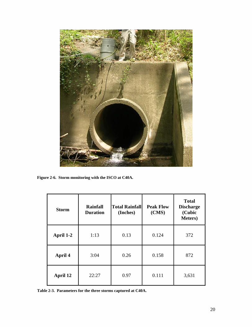
Figure 2-6. Storm monitoring with the ISCO at C40A.
Storm Rainfall Duration
Total Rainfall (Inches)
Peak Flow (CMS)
Total Discharge
(Cubic Meters)
April 1-2 1:13 0.13 0.124 372
April 4 3:04 0.26 0.158 872
April 12 22:27 0.97 0.111 3,631
Table 2-3. Parameters for the three storms captured at C40A.
20
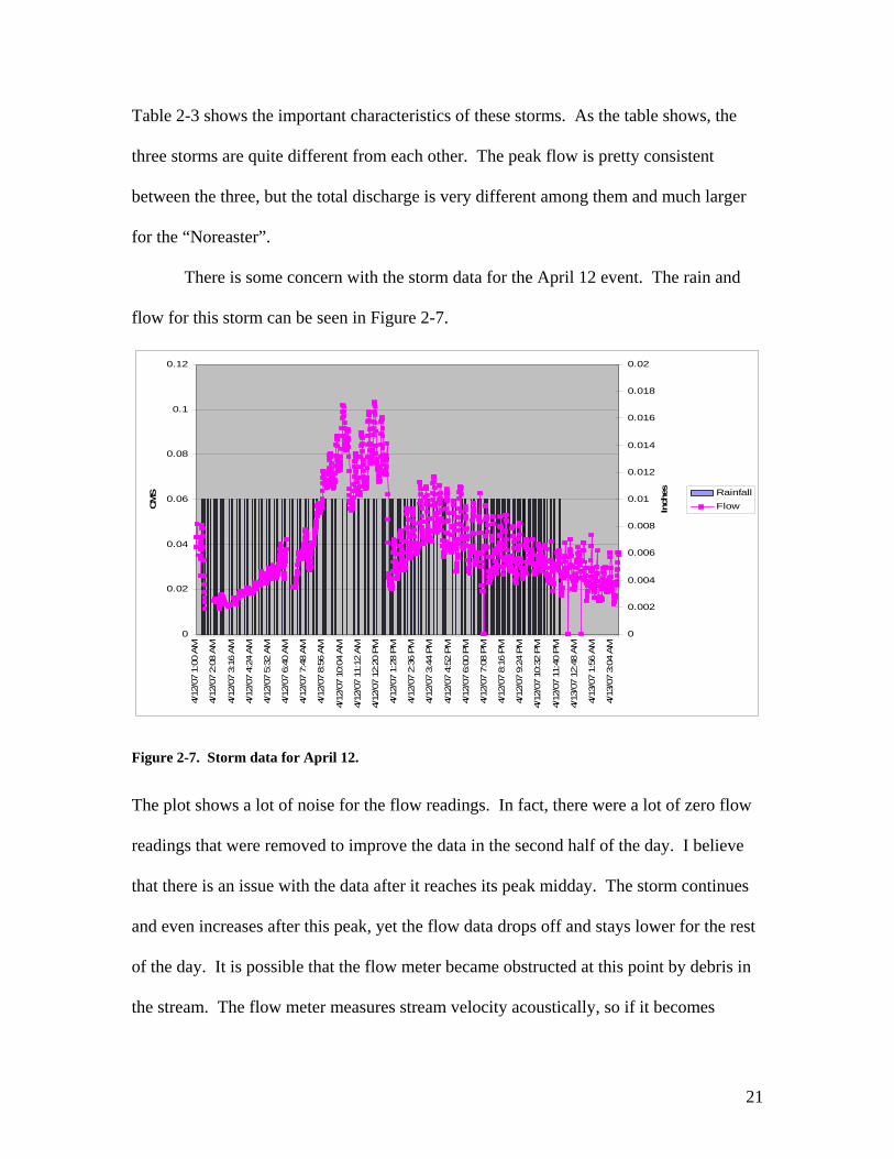
Table 2-3 shows the important characteristics of these storms. As the table shows, the
three storms are quite different from each other. The peak flow is pretty consistent
between the three, but the total discharge is very different among them and much larger
for the “Noreaster”.
There is some concern with the storm data for the April 12 event. The rain and
flow for this storm can be seen in Figure 2-7.
0
0.02
0.04
0.06
0.08
0.1
0.12
4/12
/07
1:00
AM
4/12
/07
2:08
AM
4/12
/07
3:16
AM
4/12
/07
4:24
AM
4/12
/07
5:32
AM
4/12
/07
6:40
AM
4/12
/07
7:48
AM
4/12
/07
8:56
AM
4/12
/07
10:0
4 AM
4/12
/07
11:1
2 AM
4/12
/07
12:2
0 PM
4/12
/07
1:28
PM
4/12
/07
2:36
PM
4/12
/07
3:44
PM
4/12
/07
4:52
PM
4/12
/07
6:00
PM
4/12
/07
7:08
PM
4/12
/07
8:16
PM
4/12
/07
9:24
PM
4/12
/07
10:3
2 PM
4/12
/07
11:4
0 PM
4/13
/07
12:4
8 AM
4/13
/07
1:56
AM
4/13
/07
3:04
AM
CMS
0
0.002
0.004
0.006
0.008
0.01
0.012
0.014
0.016
0.018
0.02
Inch
es RainfallFlow
Figure 2-7. Storm data for April 12.
The plot shows a lot of noise for the flow readings. In fact, there were a lot of zero flow
readings that were removed to improve the data in the second half of the day. I believe
that there is an issue with the data after it reaches its peak midday. The storm continues
and even increases after this peak, yet the flow data drops off and stays lower for the rest
of the day. It is possible that the flow meter became obstructed at this point by debris in
the stream. The flow meter measures stream velocity acoustically, so if it becomes
21

blocked or obstructed, its readings can be affected. To prevent this problem in the future,
a net could be installed upstream to try and prevent debris from reaching the meter.
Linear Programming Using the storm data, I attempted to construct a unit hydrograph3 for the C40A
site using a linear program (LP) developed from an exercise from the E66 course,
Environmental Systems. A typical modeling procedure takes the unit hydrograph storm
for a stream and computes the response for a particular storm. In this case, I am solving
the inverse problem by using storm data to construct the unit hydrograph. The LP
optimization minimizes the error between the stream flow from the data and the stream
flow determined from the unit hydrograph that is being solved for. The unit hydrograph
is the variable in the model. The error is divided into a positive and negative component
to prevent the optimization from choosing infinitely large negative errors. The continuity
constraint is a mass balance equation with a parameter K, calculated in the model from
the storm data. The K value takes into account watershed area and unit conversions. The
algebraic formulation of the model can be found in the Appendix 5. It was solved in
AMPL.
The results from the LP did not prove to be very accurate as can be seen in Table
2-4. The plots show two hydrographs for each storm. The first is the actual, which
comes from the data taken at the site. The second is produced from the unit hydrograph
developed for each storm by the LP. The first storm shows a pretty reasonable
correlation between the two curves. The other two storms, however, are off by quite a bit
in terms of the shape. There are several explanations for these discrepancies. First, the 3 Unit Hydrograph: Stream flow response to a 1” storm of a certain time length (typically ½ hour or hour long).
22
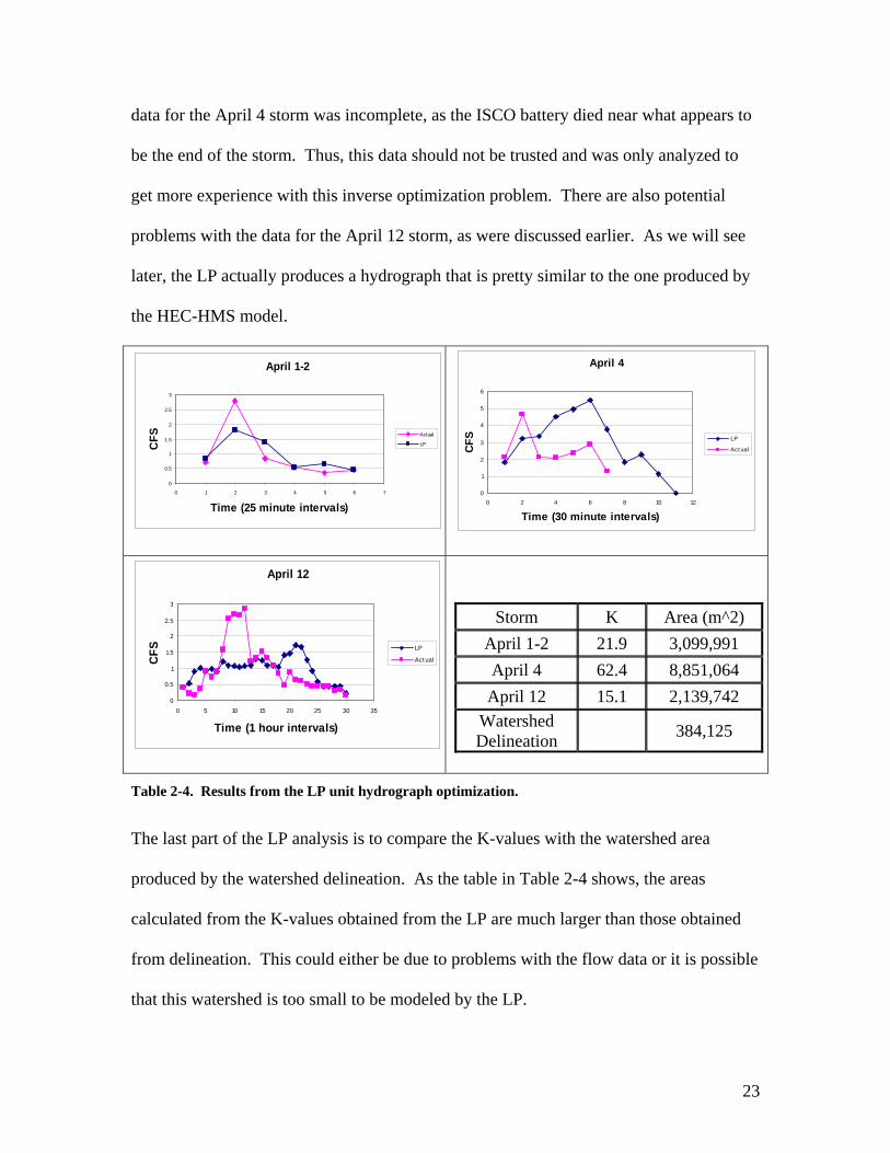
data for the April 4 storm was incomplete, as the ISCO battery died near what appears to
be the end of the storm. Thus, this data should not be trusted and was only analyzed to
get more experience with this inverse optimization problem. There are also potential
problems with the data for the April 12 storm, as were discussed earlier. As we will see
later, the LP actually produces a hydrograph that is pretty similar to the one produced by
the HEC-HMS model.
April 1-2
0
0.5
1
1.5
2
2.5
3
0 1 2 3 4 5 6 7
Time (25 minute intervals)
CFS Actual
LP
April 4
0
1
2
3
4
5
6
0 2 4 6 8 10 12
Time (30 minute intervals)
CFS LP
Act ual
April 12
0
0.5
1
1.5
2
2.5
3
0 5 10 15 20 25 30 35
Time (1 hour intervals)
CFS LP
Act ual
Storm K Area (m^2) April 1-2 21.9 3,099,991 April 4 62.4 8,851,064 April 12 15.1 2,139,742
Watershed Delineation 384,125
Table 2-4. Results from the LP unit hydrograph optimization.
The last part of the LP analysis is to compare the K-values with the watershed area
produced by the watershed delineation. As the table in Table 2-4 shows, the areas
calculated from the K-values obtained from the LP are much larger than those obtained
from delineation. This could either be due to problems with the flow data or it is possible
that this watershed is too small to be modeled by the LP.
23
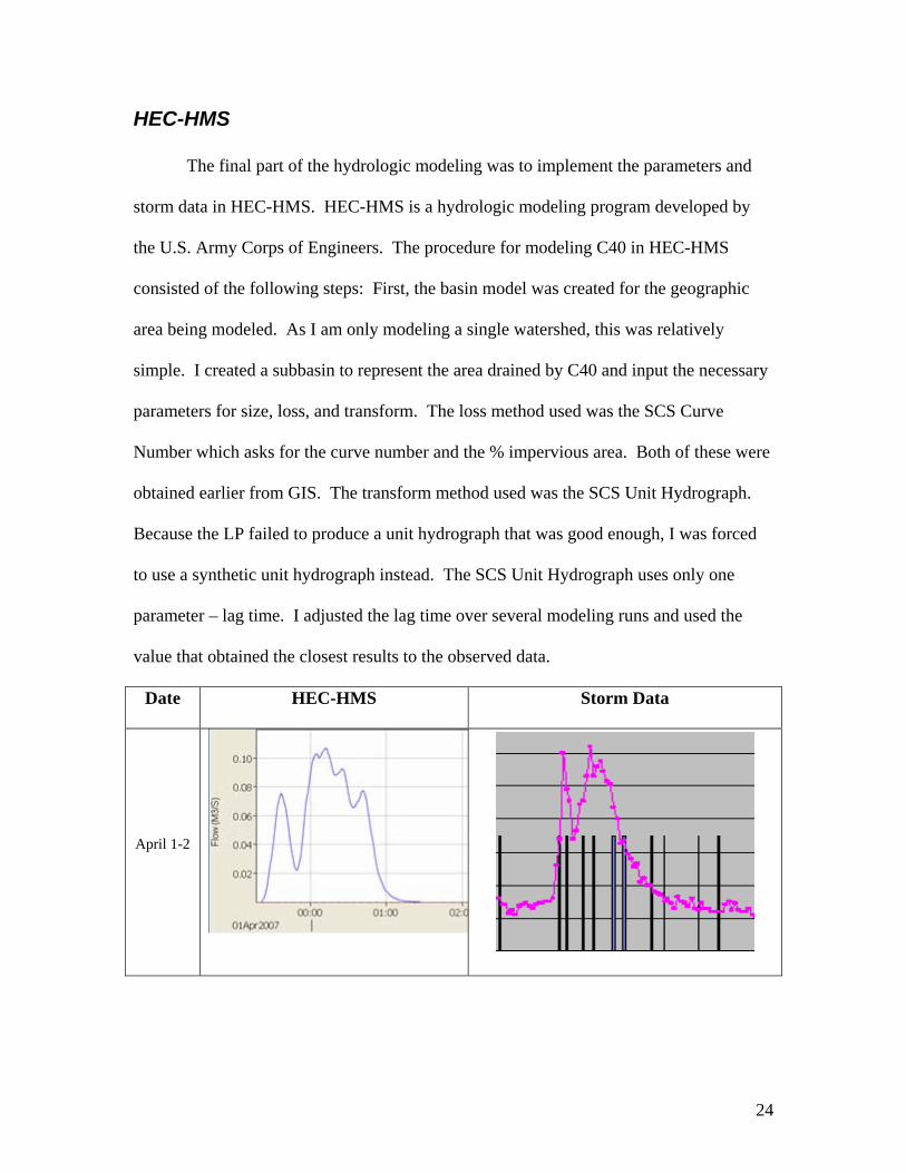
HEC-HMS The final part of the hydrologic modeling was to implement the parameters and
storm data in HEC-HMS. HEC-HMS is a hydrologic modeling program developed by
the U.S. Army Corps of Engineers. The procedure for modeling C40 in HEC-HMS
consisted of the following steps: First, the basin model was created for the geographic
area being modeled. As I am only modeling a single watershed, this was relatively
simple. I created a subbasin to represent the area drained by C40 and input the necessary
parameters for size, loss, and transform. The loss method used was the SCS Curve
Number which asks for the curve number and the % impervious area. Both of these were
obtained earlier from GIS. The transform method used was the SCS Unit Hydrograph.
Because the LP failed to produce a unit hydrograph that was good enough, I was forced
to use a synthetic unit hydrograph instead. The SCS Unit Hydrograph uses only one
parameter – lag time. I adjusted the lag time over several modeling runs and used the
value that obtained the closest results to the observed data.
Date HEC-HMS Storm Data
April 1-2
24
April 4
April 12
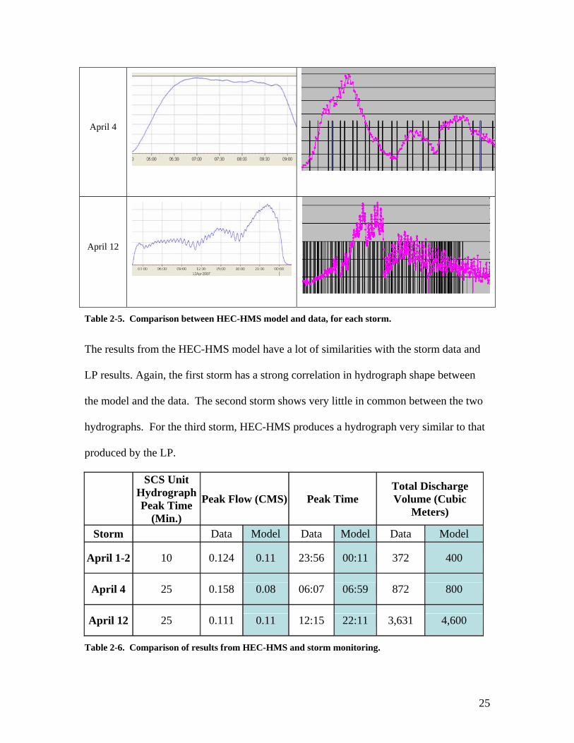
Table 2-5. Comparison between HEC-HMS model and data, for each storm.
The results from the HEC-HMS model have a lot of similarities with the storm data and
LP results. Again, the first storm has a strong correlation in hydrograph shape between
the model and the data. The second storm shows very little in common between the two
hydrographs. For the third storm, HEC-HMS produces a hydrograph very similar to that
produced by the LP.
SCS Unit Hydrograph Peak Time
(Min.)
Peak Flow (CMS) Peak Time Total Discharge Volume (Cubic
Meters)
Storm Data Model Data Model Data Model
April 1-2 10 0.124 0.11 23:56 00:11 372 400
April 4 25 0.158 0.08 06:07 06:59 872 800
April 12 25 0.111 0.11 12:15 22:11 3,631 4,600
Table 2-6. Comparison of results from HEC-HMS and storm monitoring.
25

Table 2-6 summarizes the results from the HEC-HMS models and compares them to the
data. The peak flows predicted by HEC-HMS correlate well with those observed at the
site, except for April 4. The peak times also correlate well except for April 12 when
there was possible interference in the stream flow monitoring. Finally, the total discharge
is accurate between the two which suggests that the loss method is doing a good job of
modeling the watershed. This is important because it validates the work that went into
the GIS analysis.
3. Flow and Level Control
Two key parameters involved in constructed wetland design are flow rate and water
level. The flow rate of water into the wetland impacts the hydraulic retention time, which
is the length of time water stays in the wetland. Typically, in wetland design, longer
hydraulic retention times bring greater levels of pollutant reduction. The total pollutant
loading rate on the wetland is equal to the flow rate multiplied by the pollutant
concentration.
X Q C= ∗ (3-1)
Thus, wetlands under larger flow rates are under more stress from pollutants. However,
the wetland plants require a minimum flow rate to stay healthy, so an appropriate
compromise must be maintained. Water level also has a large impact on the wetland
plants. Some plants require several inches of standing water, while others cannot survive
in such conditions. Generally, there are two types of constructed wetlands, free water
surface (FWS) and subsurface flow (SSF).
A large component of this project was to create a system for controlling these two
parameters so that they could be changed and monitored. The system that was designed
26
to do this should allow for a wide range of experimentation with flow and level at the
site. The flow and level control system functions at the inflow and outflow gates.
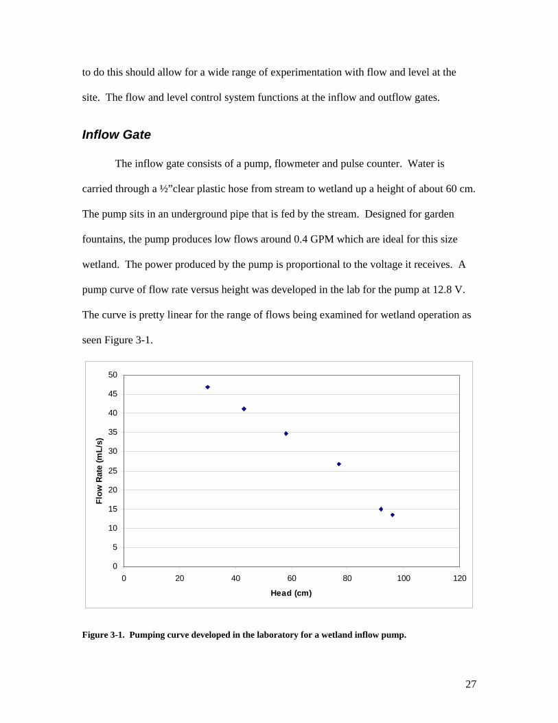
Inflow Gate The inflow gate consists of a pump, flowmeter and pulse counter. Water is
carried through a ½”clear plastic hose from stream to wetland up a height of about 60 cm.
The pump sits in an underground pipe that is fed by the stream. Designed for garden
fountains, the pump produces low flows around 0.4 GPM which are ideal for this size
wetland. The power produced by the pump is proportional to the voltage it receives. A
pump curve of flow rate versus height was developed in the lab for the pump at 12.8 V.
The curve is pretty linear for the range of flows being examined for wetland operation as
seen Figure 3-1.
0
5
10
15
20
25
30
35
40
45
50
0 20 40 60 80 100 120
Head (cm)
Flow
Rat
e (m
L/s)
Figure 3-1. Pumping curve developed in the laboratory for a wetland inflow pump.
27
As the battery is drained over long periods of pump operation, the voltage declines and
thus, so does the pumping power. Also, at the site, the level of water in the stream is
highly variable, especially during storm events. While the elevation of the wetland
receiving the pumped water remains constant, the lower elevation of the stream is
variable, and thus the height needed for pumping is variable. As flow rate is influenced
by these two factors – battery voltage and stream height – constant flow rates cannot be
assumed and a system for measuring the flows over time is needed for determining the
pollutant loadings on the wetland.
Flowmeter
Creating a system for measuring the inflow rates turned out to be one of the more
difficult tasks involved in the project. Many considerations went into choosing a
flowmeter for the system. The flow rates at the inflow are so small that they are
considered “very low flow” by flowmeter manufacturers. This factor ruled out a large
percentage of the flowmeters on the market. Another constraint on choosing a flowmeter
was the level of suspended solids in the water being measured. During storm events, the
runoff can become sediment-laden which can cause clogging and jamming of small and
intricate moving parts. The final concern was the cost of the flowmeter. Because high
accuracy was not a major concern of the project, a flowmeter was obtained at a
reasonable price with an expected error margin of 7%.
After evaluating all the options and speaking with the professionals at Omega
Engineering, the FPR-131 polypropylene paddlewheel flowmeter from Omega was
purchased for lab experimentation. This model was determined to be the best because it
was not likely to clog, was reasonably priced at about $100, and could handle low flow
28
rates with a low flow adapter. The low flow adapter is just a small piece of plastic that
sits in-between the hose and the flowmeter to lower the cross-sectional area of flow and
thus increase the velocity of flow. The higher velocity is needed at these low flow rates
to overcome the friction of the paddlewheel. The flowmeter works by rotating a
paddlewheel that stimulates a sensor each time a fin passes it. The sensor then changes
the voltage output. The voltage output alternates between the voltage the flowmeter
receives and zero. These voltage pulses are output from the meter at a rate proportional
to the flow rate.
Laboratory testing was done on the flowmeter as part of an E14/E90 collaboration
assignment. The E14 group, consisting of Susan Willis ’09, Christina Yeung ’09 and
David Kwon ’09, were handed the task of initiating the use of this flowmeter and
determining if it was practical for the job. The group began by running sediment-laden
creek samples through the device and determined that it would not fail under such
conditions. They also determined that the pressure loss from the flowmeter was not
significant and would not hamper the ability of the pump to deliver water to the wetland.
The final attribute of the flowmeter is the K-value, that is, the number of pulses to
the volume of flow. The manual provided by Omega specifies 10,900 pulses / gallon. In
basic laboratory testing I found that number to be much too high. The E14 group
determined it to be 270 pulses / gallon, but when the flowmeter was employed in the field
with the pulse counter, this conversion seemed to be a little low. It should also be noted
that the manual specifies 8” of straight pipe at the inflow of the flowmeter. This was
added when the site was setup but was not present for the calibration.
29

Pulse Counter The pulses are received by another instrument purchased from Omega, the OM-
CP PULSE101 pulse counter. Originally, a data logger from Omega’s Easy Log series
was purchased, but after laboratory testing with it, it was determined that the frequency of
pulses that it could handle was not low enough for this application. This was particularly
discouraging, as it had been recommended by an Omega professional. In the end, it
turned out that there was a small range of frequencies (25 – 50 Hz) that were
incompatible between the Easy Log pulse counter and the flowmeter. Naturally, the
frequency output for the flow rates being used happened to fall within this range, at about
37 Hz. While the Easy Log device was not functional for this application, it has many
features such as temperature, voltage and current recording options that make it a useful
instrument for the Environmental Lab.
The OM-CP pulse counter receives the pulses from the flowmeter, accumulates
them for a given time interval, records that number and then restarts the count. The
device allows the user to calibrate it so that it delivers the appropriate units rather than
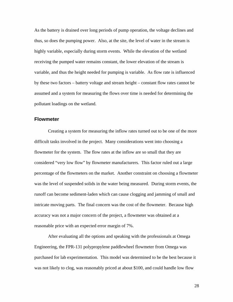
pulses, such as cubic meters / second. The pulse counter was employed in the field for a
short while when the planted channel was set up on May 2nd. Figure 3-2 shows the data
recorded by the pulse counter for about an hour after system set up. The pulses are
counted per minute and we see from the plot that they were running at about 550 pulses /
minute. This equates to 9 mL / second which is much smaller than the value of 25 mL /
second recorded using the bucket and stopwatch method by the E63 class. The pressure
drop from the flowmeter is not large enough to account for this discrepancy, thus, the
flowmeter should be calibrated in the field with the pulse counter.
30
0
100
200
300
400
500
600
700
5/2/07
4:18
PM
5/2/07
4:22
PM
5/2/07
4:26
PM
5/2/07
4:30
PM
5/2/07
4:34
PM
5/2/07
4:38
PM
5/2/07
4:42
PM
5/2/07
4:46
PM
5/2/07
4:50
PM
5/2/07
4:54
PM
5/2/07
4:58
PM
5/2/07
5:02
PM
5/2/07
5:06
PM
5/2/07
5:10
PM
5/2/07
5:14
PM
5/2/07
5:18
PM
5/2/07
5:22
PM
5/2/07
5:26
PM
5/2/07
5:30
PM
Puls
es
Figure 3-2. Pulse counter data from the field on May 2nd.
In the end, two flowmeters and two pulse counters were purchased.
Unfortunately, when the time came to install the flow monitoring system, it was
determined that one flowmeter was not functioning. Ed Jaoudi gave the meter a once-
over and could not determine the problem, so the flowmeter will have to go back to
Omega for repair or replacement.
Flow Control While inflow rate monitoring has been discussed, the system is also capable of
controlling the flow. As mentioned earlier, the pumping power is related to the voltage
received. Thus, a voltage controller could be used to control the pumping power and thus
the flow rate. Such controllers exist on the market, but could also be constructed from
simple circuitry.
31
Another method for controlling the flow is to change the height of the water being
pumped. This might be done by installing a post with several hooks at different heights
at the site, from which the hose can be raised and hung before entering the wetland.
While this method does not conserve any energy by using lower flow rates, making the
pumping height artificially higher is an effective way of lowering the flow rate and the
new flow rate can be determined quite easily from the pump curve. Obviously, with this
method flow rates could only be lowered and a stronger pump would be needed to
increase flow rates.
Outflow Gate The renovation to the outflow gate is designed to measure the flow rate out of the
system as well as control the water level in the wetland. Theoretically, the outflow rate
should be the inflow rate minus evapotranspiration. The evapotranspiration rate is
expected to be quite small according to scientific studies. The wetland is buffered from
the environment with a layer of cotton fiber reinforced rubber lining to protect the system
from leakage. Thus, we would expect the outflow rate to be very close to the inflow rate.
However, because the system was out of use for about five years, it would be nice to
verify this and determine whether there is any leaking in the system.
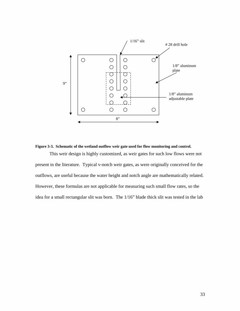
To tackle the flow measurement and level control at the outflow, a weir gate was
constructed for each channel. The aluminum weir consists of a 1/8” thick, rectangular
opening running from the top to about 2/3 of the distance down the aluminum piece. A
smaller aluminum panel was built to attach to the weir gate and cover up several heights
of the rectangular opening, allowing several options for the water level. Figure 3-3
shows a representation of the weir.
32
1/8” aluminum plate
# 28 drill hole 1/16” slit
1/8” aluminum adjustable plate
9”
8”
Figure 3-3. Schematic of the wetland outflow weir gate used for flow monitoring and control.
This weir design is highly customized, as weir gates for such low flows were not
present in the literature. Typical v-notch weir gates, as were originally conceived for the
outflows, are useful because the water height and notch angle are mathematically related.
However, these formulas are not applicable for measuring such small flow rates, so the
idea for a small rectangular slit was born. The 1/16” blade thick slit was tested in the lab
33
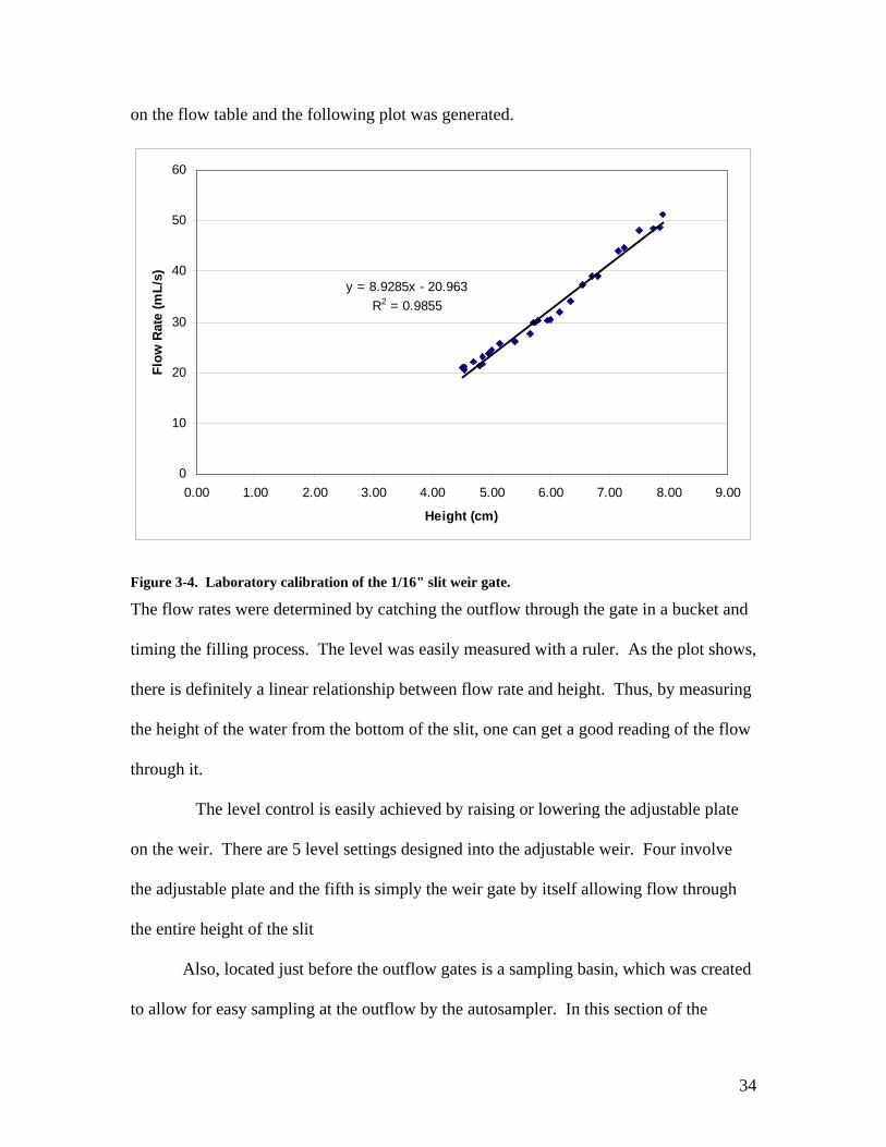
on the flow table and the following plot was generated.
y = 8.9285x - 20.963R2 = 0.9855
0
10
20
30
40
50
60
0.00 1.00 2.00 3.00 4.00 5.00 6.00 7.00 8.00 9.00
Height (cm)
Flow
Rat
e (m
L/s)
Figure 3-4. Laboratory calibration of the 1/16" slit weir gate.
The flow rates were determined by catching the outflow through the gate in a bucket and
timing the filling process. The level was easily measured with a ruler. As the plot shows,
there is definitely a linear relationship between flow rate and height. Thus, by measuring
the height of the water from the bottom of the slit, one can get a good reading of the flow
through it.
The level control is easily achieved by raising or lowering the adjustable plate
on the weir. There are 5 level settings designed into the adjustable weir. Four involve
the adjustable plate and the fifth is simply the weir gate by itself allowing flow through
the entire height of the slit
Also, located just before the outflow gates is a sampling basin, which was created
to allow for easy sampling at the outflow by the autosampler. In this section of the
34

wetland, the gravel has been removed to expose the water surface level, and a screen
should be added to prevent the gravel from refilling the basin.
Unfortunately, the installation of the weirs did not go as smoothly as planned.
When the old gates were removed, tears in the rubber lining were exposed and were
difficult to deal with. A quick fix was attempted by applying a layer of plastic sheeting
over the rubber in an attempt to patch the rips. Once the wetland was brought up to
steady state operation, it was obvious that this was not enough to prevent leakage, as
there was no flow through the weir. Thus, the weirs have not been seen in action yet at
the actual site. Solutions to this problem are probably going to entail a bit of work, as the
rubber may need to be pulled up at the end and patched from underneath. The liner also
has to be well integrated into the weir gate system, as it has to run between the weir and
the end wooden panel to make the gate watertight.
4. Solar Energy System Powering the operation of the wetland with solar energy is more sustainable and
practical than powering it off the grid. Typical wetlands, of which this is one is no
exception, are open spaces and are designed to have good southern exposure for the
plants. Thus, they are an ideal site for harnessing the sun’s rays for other purposes, such
as electric power. Solar energy is also more practical for the site because it can be
produced on-site, while electricity from the grid is not available at the site. Currently,
batteries have to be taken back to the laboratory to be charged. Hopefully, in the near
future, the plans here for a solar energy system will be expanded and acted upon.
35

Sizing Designing a solar electric system begins with sizing the system so that energy
demands are appropriately met. The text, Photovoltaic Systems Engineering4, was used
as a guide for this aspect of the design.
Electrical Load Determination The first step was to determine the load of the entire system, which includes two
pumps, two flowmeters with pulse counters, and the ISCO autosampler for sampling and
storm monitoring (rain and stream flow). The Sonde water quality measuring device was
not considered in the system because it is powered by C-size batteries, so its power is
external to the system. The pump and flowmeter loads were determined by measuring
the real-time current draws of the devices and extrapolating them to use over an entire
day to get Amp-hours / day. It is interesting that this load is slightly higher with no flow
through the flowmeter than with flow. Because the system is designed for the operating
system, I assume there is always flow through the flowmeter. The autosampler
monitoring load was reported by the device after several days of monitoring. This load
was also extrapolated to a daily load. Finally, the current draw of the autosampler was
measured for taking a 100, 200 and 500 mL sample. These were found to be 0.21, 0.21
and 0.26 Amp-hrs, respectively. The autosampler has the capacity to take 24 separate
samples, so this load was multiplied by 24 and determined to be the sampling load for a
storm event. Table 4-1 and Figure 4-1 show the loads in tabular and graphical form.
4 Messenger, Roger A. and Jerry Ventre. Photovoltaic Systems Engineering. New York: CRC Press, 2004.
36
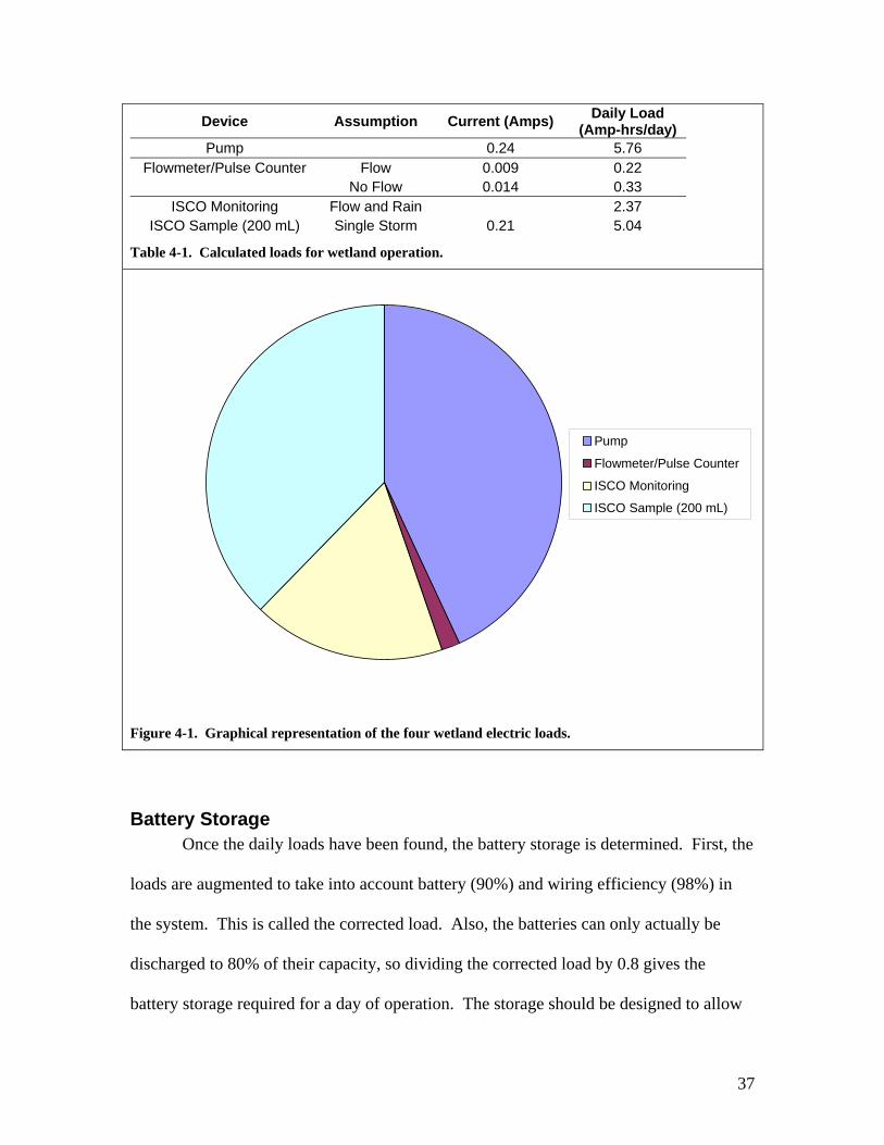
Device Assumption Current (Amps) Daily Load (Amp-hrs/day)
Pump 0.24 5.76 Flowmeter/Pulse Counter Flow 0.009 0.22
No Flow 0.014 0.33 ISCO Monitoring Flow and Rain 2.37
ISCO Sample (200 mL) Single Storm 0.21 5.04
Table 4-1. Calculated loads for wetland operation.
Pump
Flowmeter/Pulse Counter
ISCO Monitoring
ISCO Sample (200 mL)
Figure 4-1. Graphical representation of the four wetland electric loads.
Battery Storage Once the daily loads have been found, the battery storage is determined. First, the
loads are augmented to take into account battery (90%) and wiring efficiency (98%) in
the system. This is called the corrected load. Also, the batteries can only actually be
discharged to 80% of their capacity, so dividing the corrected load by 0.8 gives the
battery storage required for a day of operation. The storage should be designed to allow
37
for operation of the system for several cloudy days in which little or no solar energy can
be produced. The daily corrected load is multiplied by the number of consecutive cloudy
days to plan for, which gives the battery storage. Several scenarios were run for number
of cloudy days and number of storms to sample within the period. These can be found in
Appendix 2. The scenario of supplying power for an extra autosampler was examined as
well. In the end, the suggestion from the text was used – three cloudy days – and it was
assumed that there would only be one storm to sample within this period. This produced
a battery storage requirement of 68 Amp-hrs.
Photovoltaic (PV) Panels Finally, the required PV power output must be determined. The assumption for
this is that the entire corrected load needed for the three day cloudy period should be
supplied in a day. Thus, the daily corrected load is multiplied by the three day time
period giving a PV demand of 60.5 Amp-hrs. Assuming that, in the worst case scenario,
only four hours of peak sunlight is seen by the panels, this requires an output of about 15
Amps from the solar array. Four BP solar panels are currently available for use on the
solar array on Hicks roof. These are rated at 4.5 Amps each, so using all four would
supply the power demand of wetland operation.
Solar Array The PV panels must be installed at the site in a location where they are convenient
for wiring, difficult to reach for vandals, and of course where they will see plenty of
sunlight, particularly in the winter months. A solar pathfinder was used to find a location
with maximum exposure to sunlight. The wetland has good southern exposure, so the
ideal location is at the north end of the channels. This is conveniently at the inflow where
38
the pumps and flowmeters are located. However, as the autosampler is placed at the
outflow gates at the other end of the wetland, wiring will have to be run underground for
the length of the wetland (50 feet). There are two potential designs that have been
discussed for mounting the solar array.
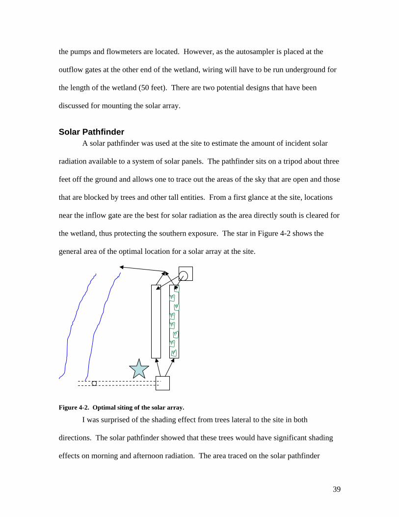
Solar Pathfinder A solar pathfinder was used at the site to estimate the amount of incident solar
radiation available to a system of solar panels. The pathfinder sits on a tripod about three
feet off the ground and allows one to trace out the areas of the sky that are open and those
that are blocked by trees and other tall entities. From a first glance at the site, locations
near the inflow gate are the best for solar radiation as the area directly south is cleared for
the wetland, thus protecting the southern exposure. The star in Figure 4-2 shows the
general area of the optimal location for a solar array at the site.
Figure 4-2. Optimal siting of the solar array.
I was surprised of the shading effect from trees lateral to the site in both
directions. The solar pathfinder showed that these trees would have significant shading
effects on morning and afternoon radiation. The area traced on the solar pathfinder
39

includes the shading of trees with leaf cover. Thus, this analysis is only really valid
between April and September. The estimation of winter radiation in this analysis is low.
Tracing the skyline, I found that the majority of solar radiation at the site is midday, peak
radiation – due to the strong southern exposure. To accommodate the worst case
scenario, the winter months, the collector tilt will be assumed at latitude + 15 degrees.
Table 4-2 shows the results from the analysis. The first column shows the average
monthly solar radiation data for Philadelphia, PA. The percent seen at the site per month
is calculated from the solar pathfinder. The final column is the product of the first two.
Month Solar Radiation at Lat. + 15 tilt5
(kWhr/m^2/day)Percent Seen (%)
Site Radiation (kWhr/m^2/day)
January 3.5 12 0.42 February 4.1 30 1.23
March 4.6 59 2.714 April 4.7 71 3.337 May 4.7 60 2.82 June 4.8 58 2.784 July 4.8 60 2.88
August 5 71 3.55 September 4.8 65 3.12
October 4.5 39 1.755 November 3.5 15 0.525 December 3.1 8 0.248
Table 4-2. Anlaysis of solar radiation at the wetland from the solar pathfinder.
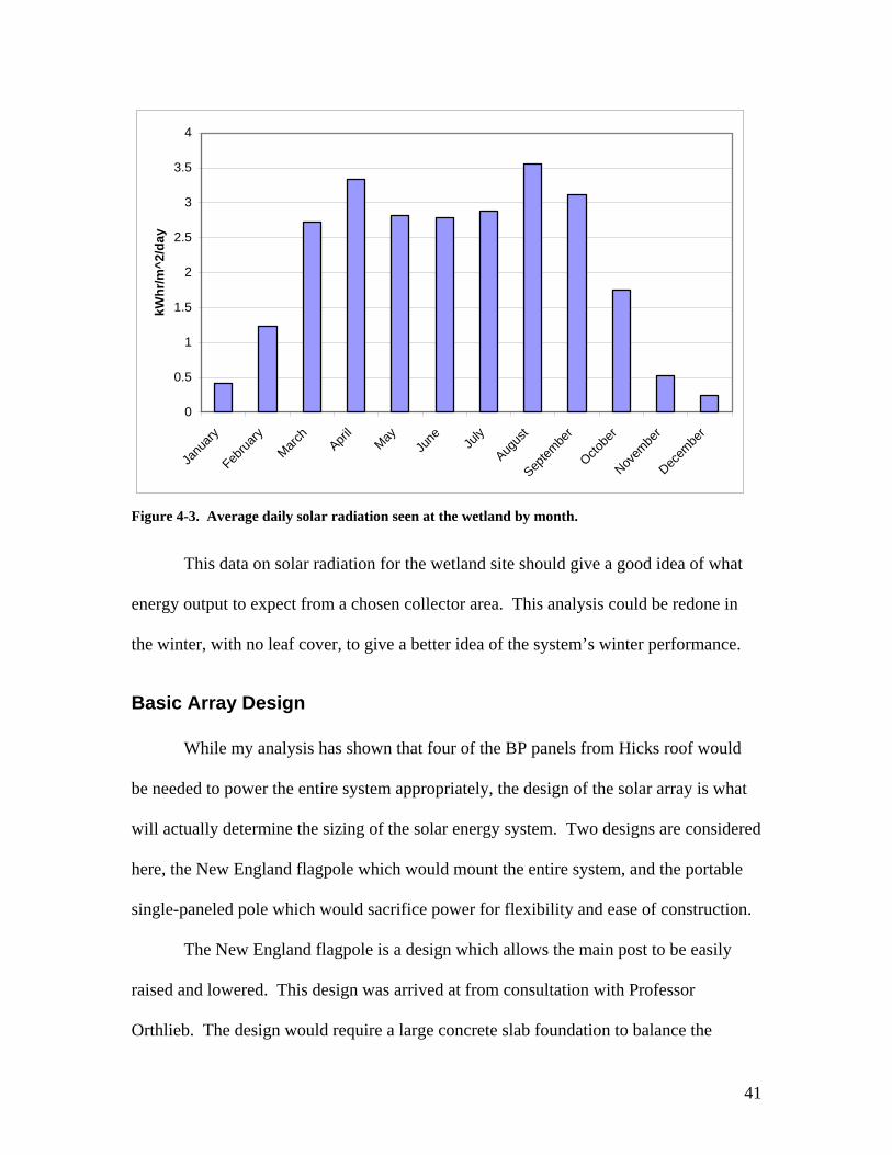
Figure 4-2 is a plot of these monthly average radiations for the wetland site.
Interestingly, the maximum average is reached in the late summer. Radiation tends to dip
midsummer due to some shading of afternoon sunlight. The winter months are very low
in solar radiation, but that is because leaf cover is assumed. In reality, they are expected
to be significantly higher.
5 Renewable Resource Data Center. http://rredc.nrel.gov/solar/old_data/nsrdb/redbook/sum2/13739.txt
40
0
0.5
1
1.5
2
2.5
3
3.5
4
Janu
ary
Februa
ryMarc
hApri
lMay
June Ju
ly
Augus
t
Septem
ber
Octobe
r
Novem
ber
Decem
ber
kWhr
/m^2
/day
Figure 4-3. Average daily solar radiation seen at the wetland by month.
This data on solar radiation for the wetland site should give a good idea of what
energy output to expect from a chosen collector area. This analysis could be redone in
the winter, with no leaf cover, to give a better idea of the system’s winter performance.
Basic Array Design While my analysis has shown that four of the BP panels from Hicks roof would
be needed to power the entire system appropriately, the design of the solar array is what
will actually determine the sizing of the solar energy system. Two designs are considered
here, the New England flagpole which would mount the entire system, and the portable
single-paneled pole which would sacrifice power for flexibility and ease of construction.
The New England flagpole is a design which allows the main post to be easily
raised and lowered. This design was arrived at from consultation with Professor
Orthlieb. The design would require a large concrete slab foundation to balance the
41

moments from wind forces on the collectors. An early estimate of the foundation is 10 –
12 cubic feet of concrete, which would probably be built at Papazian and then transported
down by machine. Rising out of the foundation are two supports which between them
hold the main post. The main post could be a wood 2 x 4 or an aluminum pole from an
old 4” light post from campus for example.
Figure 4-4. Basic representation of the New England flagpole.
As Figure 4-4 shows, the main post would be secured to the two supports through two
bolts. Removing one bolt and loosening the other allows the post to be raised or lowered
around the pivot point of the loosened bolt. The height of the post is chosen based on
several considerations. The taller the post, the more difficult the panels are to reach for
vandals and the panels have a better view of solar radiation. A taller post, however,
requires a larger foundation and is more difficult to construct and move. It was decided
that a 20 foot tall, 4” diameter aluminum pole would be ideal for the situation if it could
be found. Other potential poles include a wooden post constructed from 2 x 4 boards or a
much heavier, steel pole.
The other idea for the solar array is a more portable, single-panel installation.
This installation is more practical for the educational use of the wetland. The wetland
42

will probably not be used year-round, and when it is used, will only be for a few weeks at
a time. Thus, a solar installation that could be brought down to the site and taken away
easily when finished has its advantages. The construction would be simple, as a single
paneled could be easily attached to the top of a shorter pole. The pole could be mounted
with the cinderblock enclosure, using it as a foundation. The installation could be set up
several weeks in advance to ensure that the batteries are charged and then the pumps,
flow monitoring and ISCO could be set up at the site and run for an experiment. One
concern with this design is that the wetland should really be up and running consistently
for several months before it truly reaches steady state for pollutant removal. Thus, it
would be ideal if the system was large enough to constantly power the pumps and then
allow for some extra capacity when sampling and monitoring is desired.
5. System Performance
There have been three attempts thus far to try and quantify the performance of the
wetland in pollutant removal. Marc Jeuland obtained some preliminary results for the
wetland performance in the spring which, he warns, are not to be trusted because they
were taken too soon after planting. The E63 class analyzed wetland performance in late
November / early December, and obtained some inconclusive results. The latest results
were obtained as part of this project and echo the springtime results from Jeuland in
2001.
An important consideration in testing water quality at the site is the interferences
of other substances in the water. Interferences can severely alter readings by the
Spectrometer and Sonde. From previous experience, we know that base flow in C40 is
43

prone to much interference with nitrate readings. We know this because the method of
standard additions has been run on samples of this water and these tests have proven that
the slope and intercept of the nitrate calibration curve are abnormal. During this semester
a calibration curve was developed for this water and input into the Spectrometers,
however, a calibration curve still does not exist for the Sonde. I also learned that
different calibrations are needed for water in C40 and water in the wetland channels. It
should be noted that phosphate has proven to be much less of a problem as far as
interferences are concerned.
Latest Results On May 2nd and 4th I finally got the planted and unplanted channels, respectively,
up and flowing with C40 stream water. At this point, having only a short period of time
to run some tests on system performance, I developed three goals:
1) Determine if there is continuity between Spectrometer and Sonde readings
and improve our understanding of the interferences at the site.
2) Monitor the transient state of the wetland at startup.
3) Measure nutrient removal over the length of the wetland and compare
between the planted and unplanted channels.
Measurement Continuity and Calibration As the site is setup to have the Sonde measure the inflow and the Spectrometer
measure the outflow samples caught by the autosampler, I wanted to first determine if
water quality measurements could be compared between these different machines. As
mentioned earlier, interferences are a big problem at the site which becomes more
44
complicated because the two machines are affected differently by them. Nick Szapiro
’09 worked in the Environmental Lab this semester and constructed a calibration curve
on the Spectrometer for nitrate at C40. There was an attempt by the E63 class to calibrate
the Sonde for nitrate at C40, but due to limited time this was not fully accomplished.
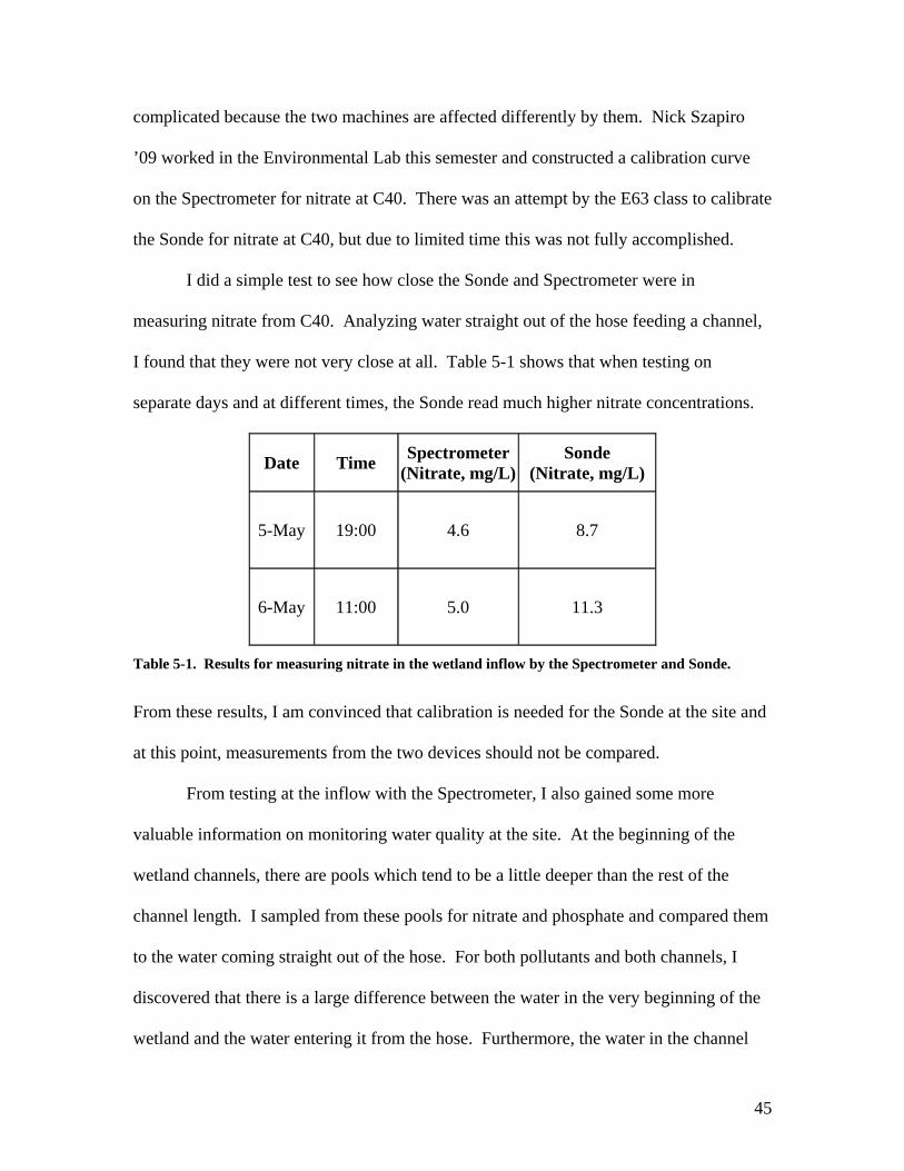
I did a simple test to see how close the Sonde and Spectrometer were in
measuring nitrate from C40. Analyzing water straight out of the hose feeding a channel,
I found that they were not very close at all. Table 5-1 shows that when testing on
separate days and at different times, the Sonde read much higher nitrate concentrations.
Date Time Spectrometer (Nitrate, mg/L)
Sonde (Nitrate, mg/L)
5-May 19:00 4.6 8.7
6-May 11:00 5.0 11.3
Table 5-1. Results for measuring nitrate in the wetland inflow by the Spectrometer and Sonde.
From these results, I am convinced that calibration is needed for the Sonde at the site and
at this point, measurements from the two devices should not be compared.
From testing at the inflow with the Spectrometer, I also gained some more
valuable information on monitoring water quality at the site. At the beginning of the
wetland channels, there are pools which tend to be a little deeper than the rest of the
channel length. I sampled from these pools for nitrate and phosphate and compared them
to the water coming straight out of the hose. For both pollutants and both channels, I
discovered that there is a large difference between the water in the very beginning of the
wetland and the water entering it from the hose. Furthermore, the water in the channel
45
was always significantly higher. Thus, it appears from this result that the water gains a
large amount of nutrients when it enters the wetland. This could be true to an extent
because there is decomposition of leaf and plant matter occurring in both channels.
However, it is very unlikely that this is causing such a rapid increase in water quality.
What is more likely is that the two waters are of a significantly different matrix and
should be calibrated separately.
Transient State When flow rates change drastically in the wetland, it takes some time for the
pollutant removal in the system to reach steady state. This period of change is the
transient state of the wetland. In this case, the wetland went from no inflow to flow
beginning on May 2nd for the planted channel. After setting up the flow for the planted
channel, I had the Sonde monitor water quality at the inflow and the autosampler take
samples every six hours. I used a six hour sampling interval because this is about the
hydraulic retention time for the wetland with the pumps as determined by the E63 class.
I predicted that after sampling for several days there would an improvement in wetland
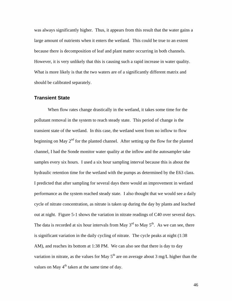
performance as the system reached steady state. I also thought that we would see a daily
cycle of nitrate concentration, as nitrate is taken up during the day by plants and leached
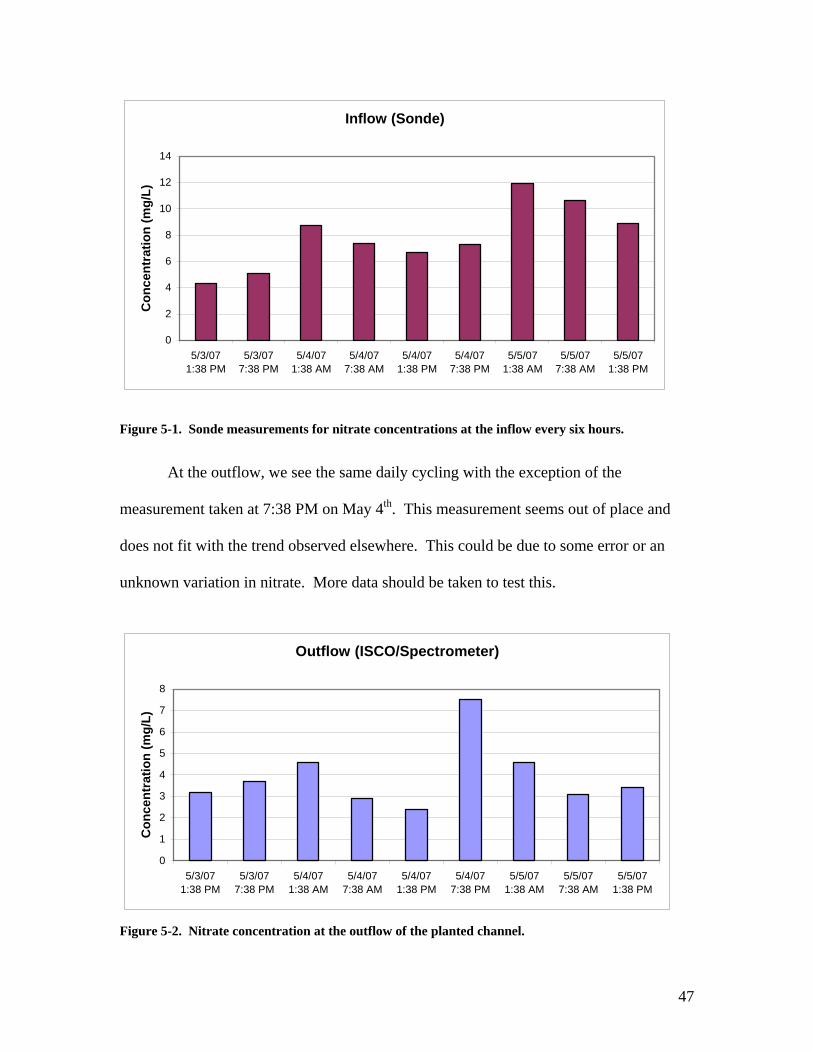
out at night. Figure 5-1 shows the variation in nitrate readings of C40 over several days.
The data is recorded at six hour intervals from May 3rd to May 5th. As we can see, there
is significant variation in the daily cycling of nitrate. The cycle peaks at night (1:38
AM), and reaches its bottom at 1:38 PM. We can also see that there is day to day
variation in nitrate, as the values for May 5th are on average about 3 mg/L higher than the
values on May 4th taken at the same time of day.
46
Inflow (Sonde)
0
2
4
6
8
10
12
14
5/3/071:38 PM
5/3/077:38 PM
5/4/071:38 AM
5/4/077:38 AM
5/4/071:38 PM
5/4/077:38 PM
5/5/071:38 AM
5/5/077:38 AM
5/5/071:38 PM
Con
cent
ratio
n (m
g/L)
Figure 5-1. Sonde measurements for nitrate concentrations at the inflow every six hours.
At the outflow, we see the same daily cycling with the exception of the
measurement taken at 7:38 PM on May 4th. This measurement seems out of place and
does not fit with the trend observed elsewhere. This could be due to some error or an
unknown variation in nitrate. More data should be taken to test this.
Outflow (ISCO/Spectrometer)
0
1
2
3
4
5
6
7
8
5/3/071:38 PM
5/3/077:38 PM
5/4/071:38 AM
5/4/077:38 AM
5/4/071:38 PM
5/4/077:38 PM
5/5/071:38 AM
5/5/077:38 AM
5/5/071:38 PM
Con
cent
ratio
n (m
g/L)
Figure 5-2. Nitrate concentration at the outflow of the planted channel.
47

The other aspect of this plot to notice is that the concentration did not rise on May 5th at
the outflow as it did at the inflow. This could indicate that the wetland is increasing its
performance for nitrate removal as time goes on and has not yet reached its steady state.
This is speculative though and should be confirmed when a proper calibration is done
with the Sonde.
Nutrient Removal over Channel Length The final and most important part of the water quality monitoring at the wetland
for this project was the measurement of nutrients at different lengths of the wetland to
determine nutrient removal. Samples were analyzed on-site by the Spectrometer for
nitrate and phosphate every day from May 3 – 6. Furthermore, they were taken at
different times of day, though not at night. They were obtained from pools at the
beginning and end of the channels and at the three intermediate sampling ports. This
sampling system divides the channel into quarters. Also, a field blank was used on the
first day for quality control. A spreadsheet in Appendix 6 shows the individual results for
each sampling time.
To determine the overall performance of the wetland in an attempt to get a single
efficiency for pollutant removal, I averaged the concentrations read at each sampling port
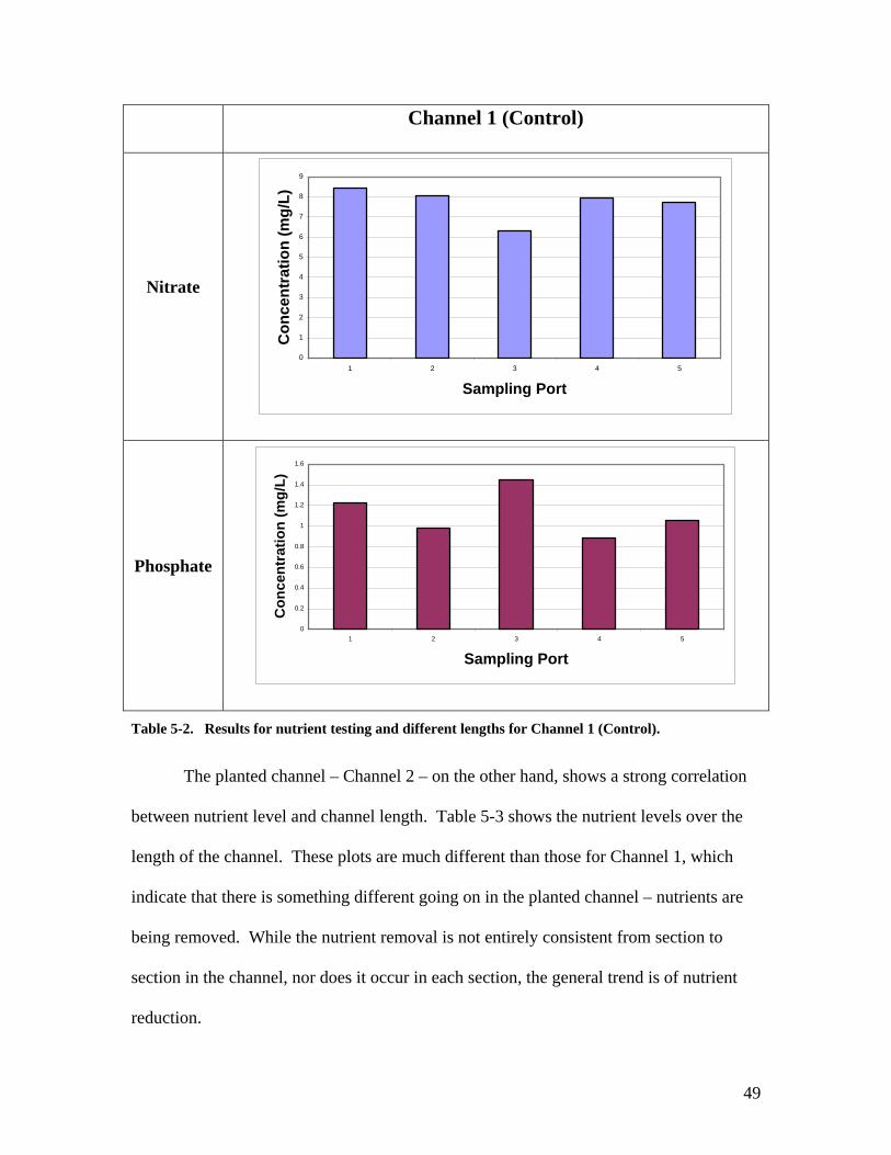
over the four-day period. Table 5-2 shows the results of this sampling in the unplanted
channel – Channel 1. The graphs show some variation between sampling ports,
particularly for phosphate. There is no general trend for the length of the channel. It
does not appear that channel length is correlated with nutrient level, and thus, nutrient
removal in the channel is insignificant.
48
Channel 1 (Control)
Nitrate
0
1
2
3
4
5
6
7
8
9
1 2 3 4 5
Sampling Port
Con
cent
ratio
n (m
g/L)
Phosphate
0
0.2
0.4
0.6
0.8
1
1.2
1.4
1.6
1 2 3 4 5
Sampling Port
Con
cent
ratio
n (m
g/L)
Table 5-2. Results for nutrient testing and different lengths for Channel 1 (Control).
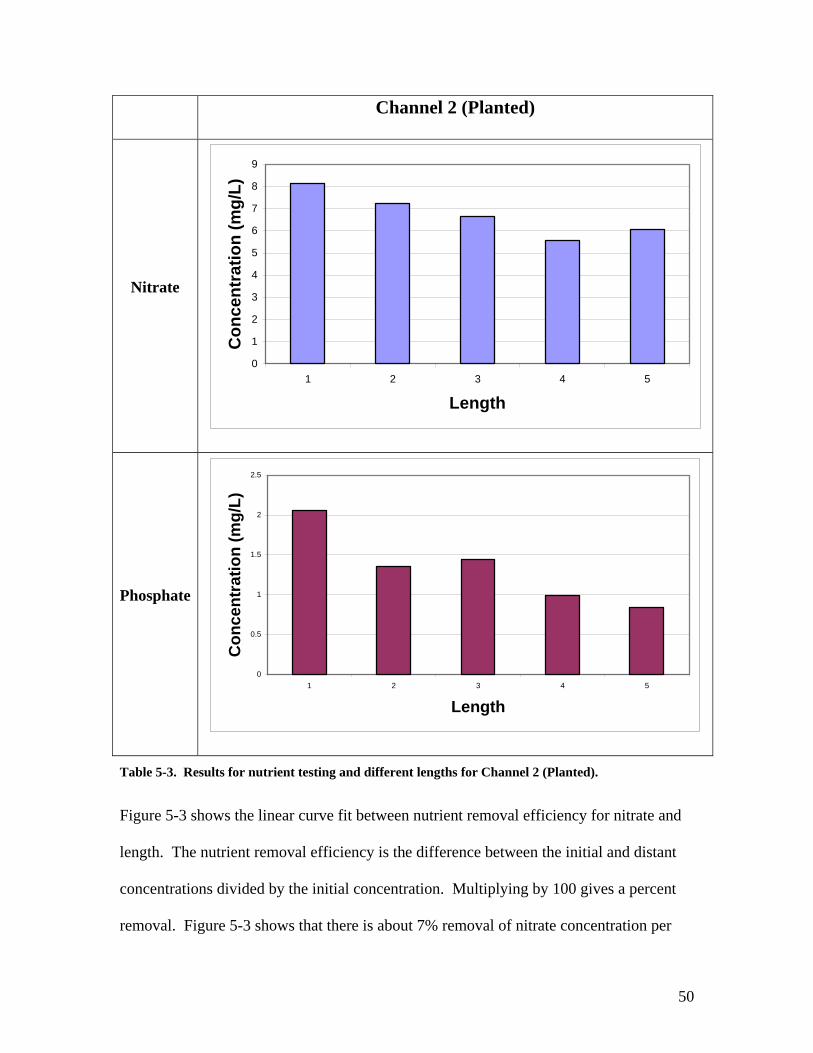
The planted channel – Channel 2 – on the other hand, shows a strong correlation
between nutrient level and channel length. Table 5-3 shows the nutrient levels over the
length of the channel. These plots are much different than those for Channel 1, which
indicate that there is something different going on in the planted channel – nutrients are
being removed. While the nutrient removal is not entirely consistent from section to
section in the channel, nor does it occur in each section, the general trend is of nutrient
reduction.
49
Channel 2 (Planted)
Nitrate
0
1
2
3
4
5
6
7
8
9
1 2 3 4 5
Length
Con
cent
ratio
n (m
g/L)
Phosphate
0
0.5
1
1.5
2
2.5
1 2 3 4 5
Length
Con
cent
ratio
n (m
g/L)
Table 5-3. Results for nutrient testing and different lengths for Channel 2 (Planted).
Figure 5-3 shows the linear curve fit between nutrient removal efficiency for nitrate and
length. The nutrient removal efficiency is the difference between the initial and distant
concentrations divided by the initial concentration. Multiplying by 100 gives a percent
removal. Figure 5-3 shows that there is about 7% removal of nitrate concentration per
50
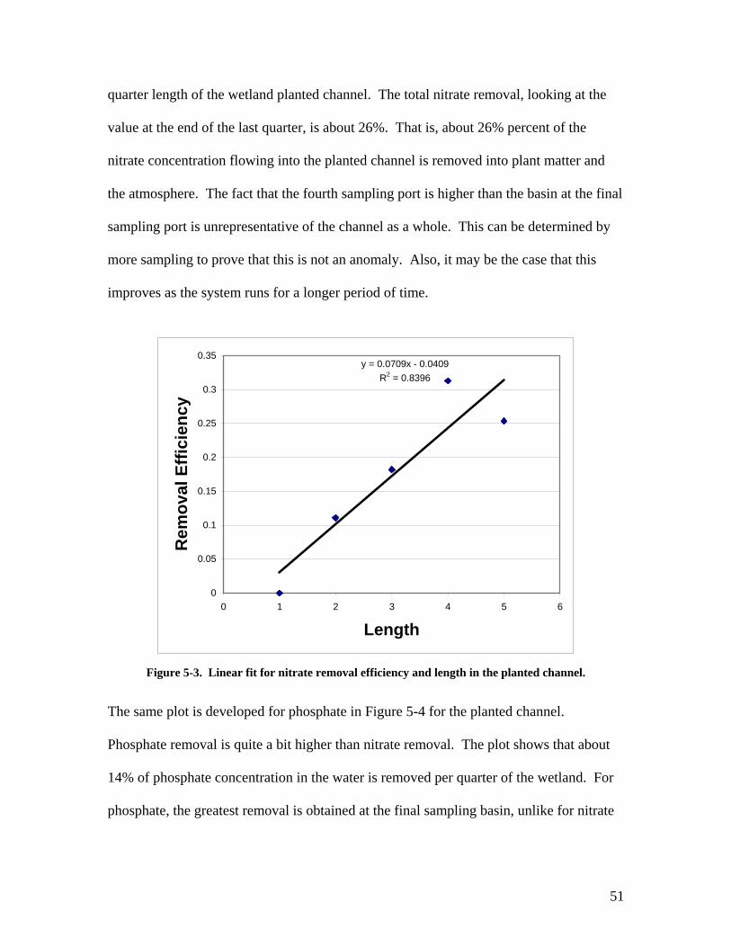
quarter length of the wetland planted channel. The total nitrate removal, looking at the
value at the end of the last quarter, is about 26%. That is, about 26% percent of the
nitrate concentration flowing into the planted channel is removed into plant matter and
the atmosphere. The fact that the fourth sampling port is higher than the basin at the final
sampling port is unrepresentative of the channel as a whole. This can be determined by
more sampling to prove that this is not an anomaly. Also, it may be the case that this
improves as the system runs for a longer period of time.
y = 0.0709x - 0.0409R2 = 0.8396
0
0.05
0.1
0.15
0.2
0.25
0.3
0.35
0 1 2 3 4 5
Length
Rem
oval
Effi
cien
cy
6
Figure 5-3. Linear fit for nitrate removal efficiency and length in the planted channel.
The same plot is developed for phosphate in Figure 5-4 for the planted channel.
Phosphate removal is quite a bit higher than nitrate removal. The plot shows that about
14% of phosphate concentration in the water is removed per quarter of the wetland. For
phosphate, the greatest removal is obtained at the final sampling basin, unlike for nitrate
51
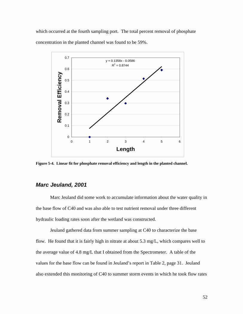
which occurred at the fourth sampling port. The total percent removal of phosphate
concentration in the planted channel was found to be 59%.
y = 0.1358x - 0.0586R2 = 0.8744
0
0.1
0.2
0.3
0.4
0.5
0.6
0.7
0 1 2 3 4 5
Length
Rem
oval
Effi
cien
cy
6
Figure 5-4. Linear fit for phosphate removal efficiency and length in the planted channel.
Marc Jeuland, 2001 Marc Jeuland did some work to accumulate information about the water quality in
the base flow of C40 and was also able to test nutrient removal under three different
hydraulic loading rates soon after the wetland was constructed.
Jeuland gathered data from summer sampling at C40 to characterize the base
flow. He found that it is fairly high in nitrate at about 5.3 mg/L, which compares well to
the average value of 4.8 mg/L that I obtained from the Spectrometer. A table of the
values for the base flow can be found in Jeuland’s report in Table 2, page 31. Jeuland
also extended this monitoring of C40 to summer storm events in which he took flow rates
52

and concentrations and calculated average and maximum loadings. Again, these figures
can be found in his report on page 32.
In 2001, soon after planting the wetland, Jeuland did a preliminary nutrient
removal analysis for the wetland. He ran the wetland under three different hydraulic
loading rates and averaged the nutrient removal. For the planted channel, he obtained
46.4% nitrate removal and 48% phosphate removal. Table 5-4 compares the
concentration percent removals for 2001 and this project.
NNiittrraattee PPhhoosspphhaattee
2001 (Jeuland)
2007 (Bangs)
2001 (Jeuland)
2007 (Bangs)
Removal % per quarter
section 11.6% 7% 12.0% 14%
Table 5-4. Comparison of results obtained in 2001 and 2007 for nutrient removal in the planted channel.
Jeuland also quoted values of 2.4% and 8.9% per quarter section for nitrate and
phosphate, respectively, for the unplanted channel. I found these values to be negligible
from my testing because the outflow concentration was not significantly lower than the
inflow and there was no correlation between concentration and channel length.
53
E63, Fall 2006 The report produced by the fall, 2006, E63 class is in the possession of Professor
McGarity. The report outlines some interesting results in the third section on system
performance.
The class tracked four separate storm events and obtained data on concentrations
in C40. Flow rates were not monitored, so pollutant loadings could not be determined as
they were by Jeuland in 2001. The main findings for the storm events were a strong
negative correlation between turbidity and specific conductivity and a weak correlation
between specific conductivity and nitrate.
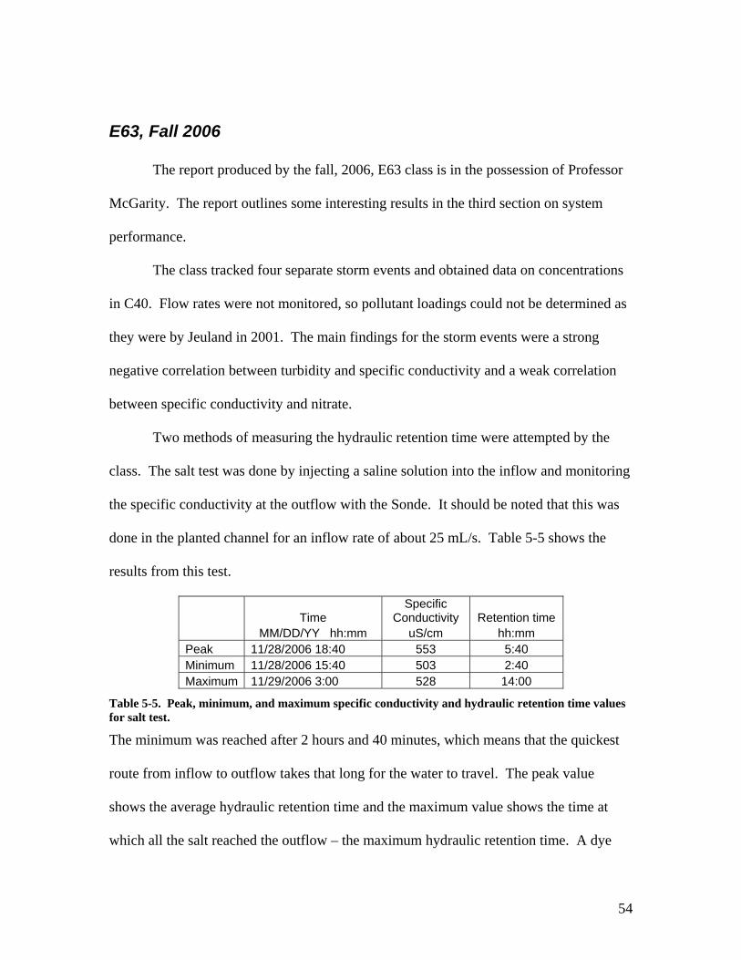
Two methods of measuring the hydraulic retention time were attempted by the
class. The salt test was done by injecting a saline solution into the inflow and monitoring
the specific conductivity at the outflow with the Sonde. It should be noted that this was
done in the planted channel for an inflow rate of about 25 mL/s. Table 5-5 shows the
results from this test.
Time Specific
Conductivity Retention time MM/DD/YY hh:mm uS/cm hh:mm Peak 11/28/2006 18:40 553 5:40 Minimum 11/28/2006 15:40 503 2:40 Maximum 11/29/2006 3:00 528 14:00
Table 5-5. Peak, minimum, and maximum specific conductivity and hydraulic retention time values for salt test.
The minimum was reached after 2 hours and 40 minutes, which means that the quickest
route from inflow to outflow takes that long for the water to travel. The peak value
shows the average hydraulic retention time and the maximum value shows the time at
which all the salt reached the outflow – the maximum hydraulic retention time. A dye
54
test was attempted with the Sonde to read the turbidity from the dye in the water.
However, the readings were not high enough to produce firm results.
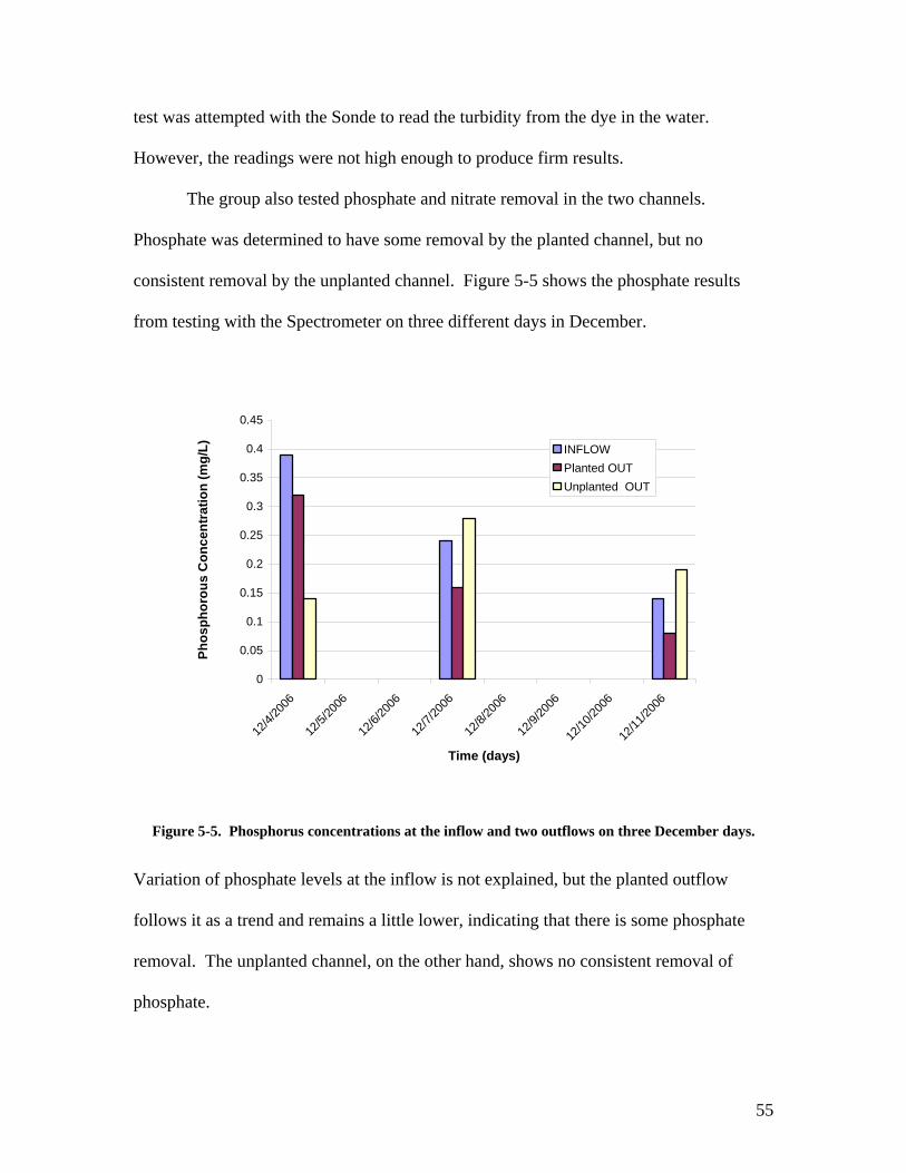
The group also tested phosphate and nitrate removal in the two channels.
Phosphate was determined to have some removal by the planted channel, but no
consistent removal by the unplanted channel. Figure 5-5 shows the phosphate results
from testing with the Spectrometer on three different days in December.
0
0.05
0.1
0.15
0.2
0.25
0.3
0.35
0.4
0.45
12/4/
2006
12/5/
2006
12/6/
2006
12/7/
2006
12/8/
2006
12/9/
2006
12/10
/2006
12/11
/2006
Time (days)
Phos
phor
ous
Con
cent
ratio
n (m
g/L) INFLOW
Planted OUTUnplanted OUT
Figure 5-5. Phosphorus concentrations at the inflow and two outflows on three December days.
Variation of phosphate levels at the inflow is not explained, but the planted outflow
follows it as a trend and remains a little lower, indicating that there is some phosphate
removal. The unplanted channel, on the other hand, shows no consistent removal of
phosphate.
55
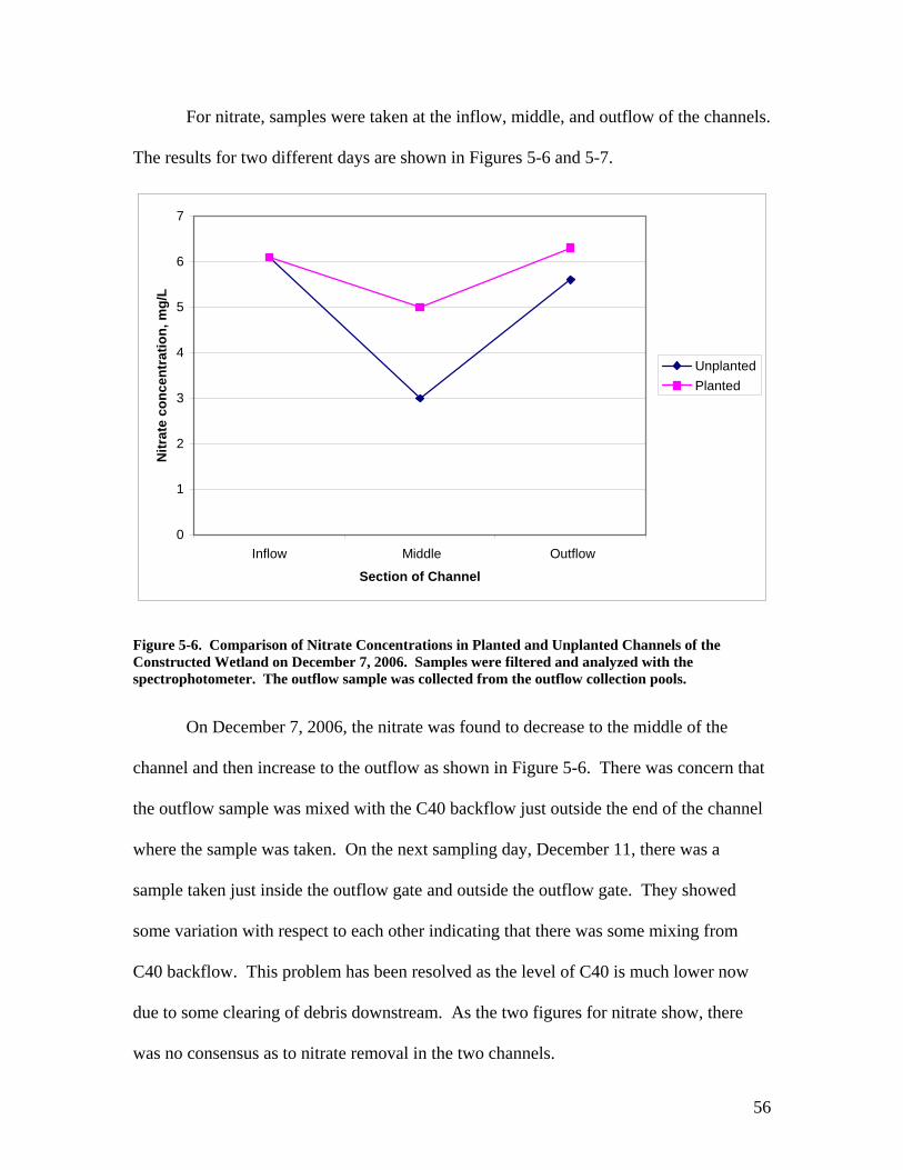
For nitrate, samples were taken at the inflow, middle, and outflow of the channels.
The results for two different days are shown in Figures 5-6 and 5-7.
0
1
2
3
4
5
6
7
Inflow Middle Outflow
Section of Channel
Nitr
ate
conc
entr
atio
n, m
g/L
UnplantedPlanted
Figure 5-6. Comparison of Nitrate Concentrations in Planted and Unplanted Channels of the Constructed Wetland on December 7, 2006. Samples were filtered and analyzed with the spectrophotometer. The outflow sample was collected from the outflow collection pools.
On December 7, 2006, the nitrate was found to decrease to the middle of the
channel and then increase to the outflow as shown in Figure 5-6. There was concern that
the outflow sample was mixed with the C40 backflow just outside the end of the channel
where the sample was taken. On the next sampling day, December 11, there was a
sample taken just inside the outflow gate and outside the outflow gate. They showed
some variation with respect to each other indicating that there was some mixing from
C40 backflow. This problem has been resolved as the level of C40 is much lower now
due to some clearing of debris downstream. As the two figures for nitrate show, there
was no consensus as to nitrate removal in the two channels.
56

0
2
4
6
8
10
12
Inflow Middle Outflow (inner) Outlflow (outer)
Section of Channel
Nitr
ate
conc
entr
atio
n, m
g/L
UnplantedPlanted
Figure 5-7. Comparison of Nitrate Concentrations in Planted and Unplanted Channels of the Constructed Wetland on December 11, 2006. Samples were filtered and analyzed with the spectrophotometer. Outflow samples were collected from inside the end of each trench and from the outflow collection pools.
6. Conclusion and Future Work
Realistic Design Constraints These are the design constraints that I faced in my project specifically on
improving the constructed wetland at Swarthmore College. For realistic design
constraints for the construction and maintenance of the wetland, one should consult Marc
Jeuland’s report, page 44.
57

Economic As with most E90 projects, this project was limited by the monetary budget. It
would have been ideal to be able to purchase two more Sondes for a total of three. This
would allow simultaneous unattended sampling at the inflow and at one point in each
channel. Cost was also a key consideration in purchasing a flow monitoring system at the
wetland inflow.
Environmental Because the site is located in a natural wetland, there are limitations as to what
can be done. All installations there should be temporary. This includes the cinder block
enclosures, pumping and monitoring system. This was also a consideration for designing
the solar energy system. Mounting a solar array into the ground was decided against
because it would be difficult to remove. Instead, if the entire array is built, a portable
concrete foundation should be used or the cinder block enclosures could be used in some
capacity.
Sustainability Sustainability is at the heart of this project. As a natural method for water
treatment, the idea of the site is to be a sustainable alternative to conventional water
treatment methods. There is also the hope that the site will become almost completely
sustainable by using solar panels to power the electrical devices needed for the operation
and monitoring of the wetland.
58

Manufacturability Constructing and installing the weirs at the outflow gates was a large part of the
project and turned out to be one of the most constrained tasks. Working at the outflow is
particularly difficult because it is very muddy and difficult to move. The weirs had to be
integrated into the old wetland structure, which was found to be deteriorating. The
rubber lining at the outflow had been damaged and rips were increased as work was
undertaken. In the end, this work turned out to be unsuccessful and this task will have to
be passed on to the next wetland steward.
Ethical The ethical concerns are largely environmental for this project. I believe the
general consensus would be that this is an ethical project.
Health and Safety Clearing the site and C40 downstream of the wetland required the use of a
chainsaw for which I partnered with Perry Carlson ’08. The batteries are a potential
source of environmental contamination and should be dealt with accordingly. They are
also very heavy and bulky, so transportation is a safety risk. Laboratory reagents can be
harmful to the environment, so they should be carefully used in the field and properly
disposed of in the lab.
Cost Summary Flowmeters (2) Omega FPR-131 $199.00 Pulse Counters (2) Omega CP-PULSE101 $400.00 Data Logger Omega OM-EL-2 $185.00 Total $885.00
59

Future Work There is still a lot of work that can be done to turn the wetland into a more
capable experimental facility. The future plans for the site look optimistic, as there will
be several high school students and teachers on staff in the Environmental Lab this
summer as part of the HHMI program. Future work exists in all four sections of this
project.
Hydrologic Modeling
• Monitor more storms at C40A and find a way to protect debris from piling up on the flow meter.
• Determine the unit hydrograph for C40A • Continue HEC-HMS modeling with new data, verify with storm monitoring
Flow and Level Control
• Create a watertight seal on the outflow integrated with the weir gates in place • Calibrate weir gates in the field • Create system to adjust inflow rates • Experiment with different levels and flows in the wetland
Solar Energy System
• Test BP photovoltaic panels on the Hicks roof • Choose array design and construct it • Monitor performance of the system
Wetland Performance
• Continue seeking nutrient removal efficiencies • Permit the system to run for longer periods (weeks) before testing performance • Monitor conditions of the plants, keep the unplanted channel clear • Approximate wetland area required to treat the entirety of C40
60

Acknowledgements I would like to thank everyone that was involved with this project, this was not a
one man show by any means:
Professor Arthur McGarity, my advisor, for his support and advice and helping to keep the project moving forward. Grant “Smitty” Smith, for his expert help in the engineering shop and for letting me use the truck virtually whenever. Professor Fred Orthlieb, for his ideas and knowledge about the solar array. Ed Jaoudi, for his help with everything electric. Fall E63 Classmates: Scott Fortmann-Roe, Kaitlin Friedman (Bryn Mawr), Edward Goldstein, Laurn Goodfriend, Jessica Mandrick, Karina Navarro, Lauren Richie, Kelly Siano, for getting the project jump-started in the fall. E14 Collaborators: David Nuri Kwon, Susan Willis, Tina Yeung, for their fine work on bringing the Omega flow meter into operation. Perry Carlson, for his brawn in helping to clear the site and to help with stream repairs. Nick Szapiro, for his work in the lab to try and help figure out this calibration madness. Also, for helping to run samples as time was coming down to the wire.
Appendix
1. GIS determination of open spaces in the C40A watershed 2. Solar energy system calculations spreadsheet 3-4. Storm data collected at C40A (April 12th data is in Figure 2-7) 5. Linear programming formulation for unit hydrograph determination 6. Nutrient monitoring spreadsheet
There are several files of interest located on the Delaware server at: \\delaware\elabusr_home\y07_ColtonE90
61
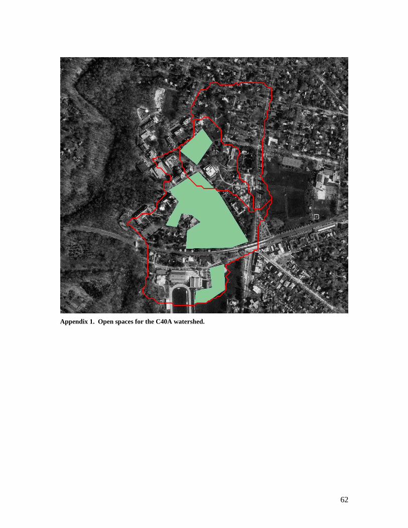
Appendix 1. Open spaces for the C40A watershed.
62
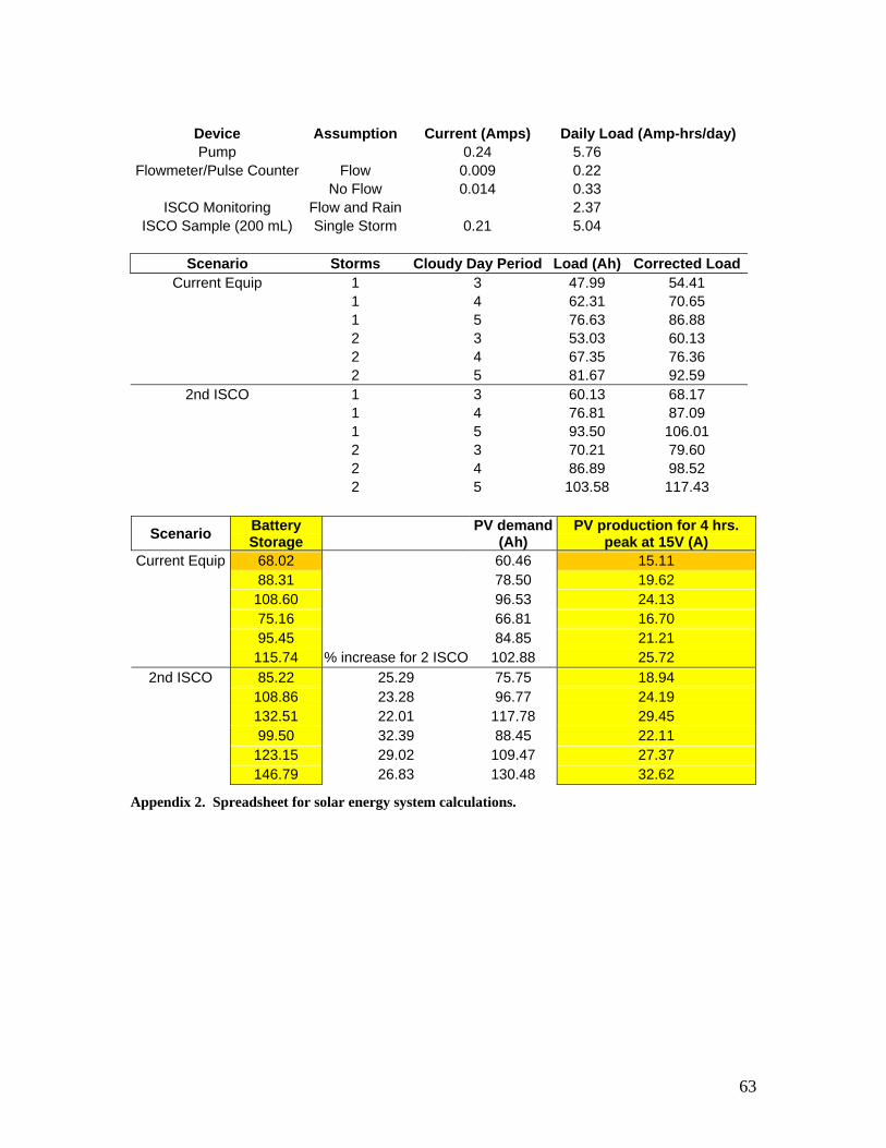
Device Assumption Current (Amps) Daily Load (Amp-hrs/day) Pump 0.24 5.76
Flowmeter/Pulse Counter Flow 0.009 0.22 No Flow 0.014 0.33
ISCO Monitoring Flow and Rain 2.37 ISCO Sample (200 mL) Single Storm 0.21 5.04
Scenario Storms Cloudy Day Period Load (Ah) Corrected Load
Current Equip 1 3 47.99 54.41 1 4 62.31 70.65 1 5 76.63 86.88 2 3 53.03 60.13 2 4 67.35 76.36 2 5 81.67 92.59
2nd ISCO 1 3 60.13 68.17 1 4 76.81 87.09 1 5 93.50 106.01 2 3 70.21 79.60 2 4 86.89 98.52 2 5 103.58 117.43
Scenario Battery
Storage PV demand (Ah)
PV production for 4 hrs. peak at 15V (A)
Current Equip 68.02 60.46 15.11 88.31 78.50 19.62 108.60 96.53 24.13 75.16 66.81 16.70 95.45 84.85 21.21 115.74 % increase for 2 ISCO 102.88 25.72
2nd ISCO 85.22 25.29 75.75 18.94 108.86 23.28 96.77 24.19 132.51 22.01 117.78 29.45 99.50 32.39 88.45 22.11 123.15 29.02 109.47 27.37 146.79 26.83 130.48 32.62
Appendix 2. Spreadsheet for solar energy system calculations.
63
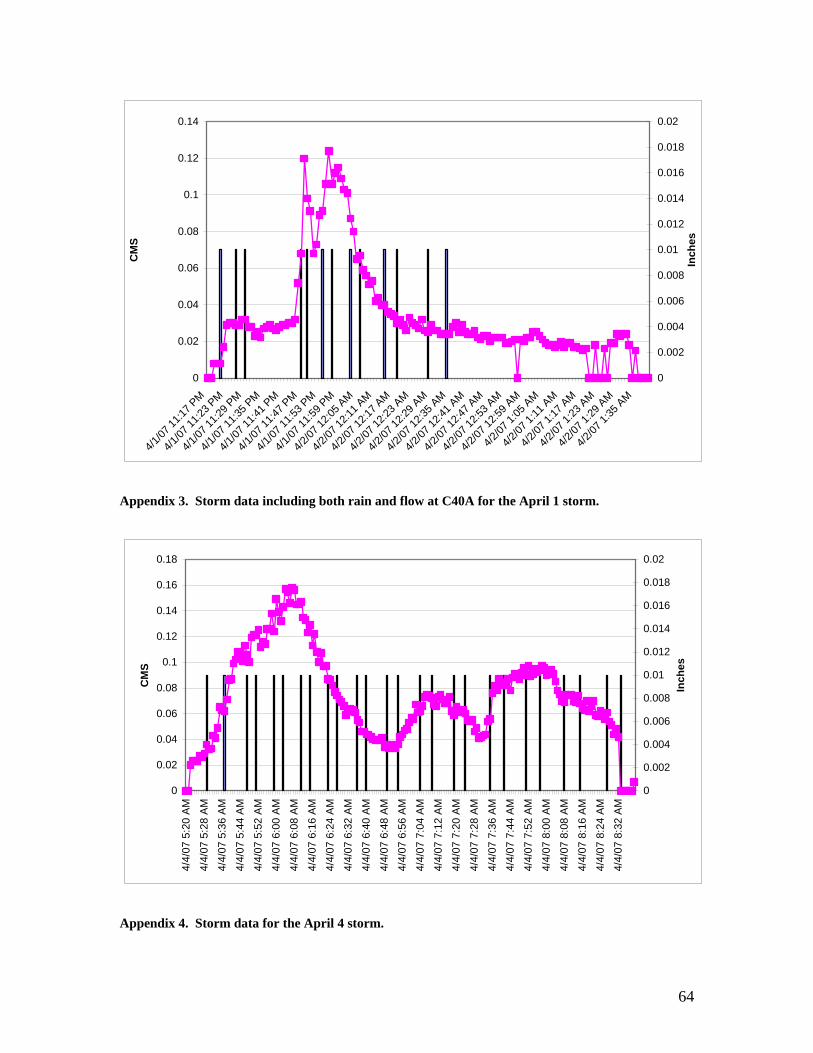
0
0.02
0.04
0.06
0.08
0.1
0.12
0.14
4/1/07
11:17
PM
4/1/07
11:23
PM
4/1/07
11:29
PM
4/1/07
11:35
PM
4/1/07
11:41
PM
4/1/07
11:47
PM
4/1/07
11:53
PM
4/1/07
11:59
PM
4/2/07
12:05
AM
4/2/07
12:11
AM
4/2/07
12:17
AM
4/2/07
12:23
AM
4/2/07
12:29
AM
4/2/07
12:35
AM
4/2/07
12:41
AM
4/2/07
12:47
AM
4/2/07
12:53
AM
4/2/07
12:59
AM
4/2/07
1:05
AM
4/2/07
1:11
AM
4/2/07
1:17
AM
4/2/07
1:23
AM
4/2/07
1:29
AM
4/2/07
1:35
AM
CM
S
0
0.002
0.004
0.006
0.008
0.01
0.012
0.014
0.016
0.018
0.02
Inch
es
Appendix 3. Storm data including both rain and flow at C40A for the April 1 storm.
0
0.02
0.04
0.06
0.08
0.1
0.12
0.14
0.16
0.18
4/4/
07 5
:20
AM
4/4/
07 5
:28
AM
4/4/
07 5
:36
AM
4/4/
07 5
:44
AM
4/4/
07 5
:52
AM
4/4/
07 6
:00
AM
4/4/
07 6
:08
AM
4/4/
07 6
:16
AM
4/4/
07 6
:24
AM
4/4/
07 6
:32
AM
4/4/
07 6
:40
AM
4/4/
07 6
:48
AM
4/4/
07 6
:56
AM
4/4/
07 7
:04
AM
4/4/
07 7
:12
AM
4/4/
07 7
:20
AM
4/4/
07 7
:28
AM
4/4/
07 7
:36
AM
4/4/
07 7
:44
AM
4/4/
07 7
:52
AM
4/4/
07 8
:00
AM
4/4/
07 8
:08
AM
4/4/
07 8
:16
AM
4/4/
07 8
:24
AM
4/4/
07 8
:32
AM
CM
S
0
0.002
0.004
0.006
0.008
0.01
0.012
0.014
0.016
0.018
0.02
Inch
es
Appendix 4. Storm data for the April 4 storm.
64

Appendix 5. Linear program for determining a unit hydrograph by solving the inverse problem.
65
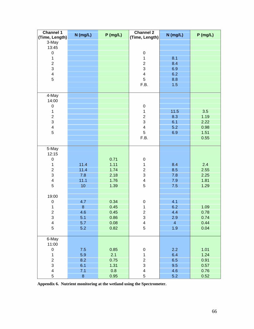
Channel 1 (Time, Length) N (mg/L) P (mg/L) Channel 2
(Time, Length) N (mg/L) P (mg/L)
3-May 13:45
0 0 1 1 8.1 2 2 8.4 3 3 6.9 4 4 6.2 5 5 8.8 F .B. 1.5
4-May 14:00
0 0 1 1 11.5 3.5 2 2 8.3 1.19 3 3 6.1 2.22 4 4 5.2 0.98 5 5 6.9 1.51 F .B. 0.55
5-May 12:15
0 0.71 0 1 11.4 1.11 1 8.4 2.4 2 11.4 1.74 2 8.5 2.55 3 7.8 2.18 3 7.8 2.25 4 11.1 1.76 4 7.9 1.81 5 10 1.39 5 7.5 1.29
19:00 0 4.7 0.34 0 4.1 1 8 0.45 1 6.2 1.09 2 4.6 0.45 2 4.4 0.78 3 5.1 0.86 3 2.9 0.74 4 5.7 0.08 4 4 0.44 5 5.2 0.82 5 1.9 0.04
6-May 11:00
0 7.5 0.85 0 2.2 1.01 1 5.9 2.1 1 6.4 1.24 2 8.2 0.75 2 6.5 0.91 3 6.1 1.31 3 9.5 0.57 4 7.1 0.8 4 4.6 0.76 5 8 0.95 5 5.2 0.52
Append 6. Nutrient monitoring at the d using the Spectrometer. ix wetlan
66

67