Upscaling of Geocellular Models for Flow Simulation

Louis J. Durlofsky

Department of Petroleum Engineering, Stanford University

ChevronTexaco ETC, San Ramon, CA

2

Acknowledgments

• Yuguang Chen (Stanford University)

• Mathieu Prevost (now at Total)

• Xian-Huan Wen (ChevronTexaco)

• Yalchin Efendiev (Texas A&M)

(photo by Eric Flodin)

3

• Issues and existing techniques

• Adaptive local-global upscaling

• Velocity reconstruction and multiscale solution

• Generalized convection-diffusion transport model

• Upscaling and flow-based grids (3D unstructured)

• Outstanding issues and summary

Outline

4

Requirements/Challenges for Upscaling

• Accuracy & Robustness

– Retain geological realism in flow simulation

– Valid for different types of reservoir heterogeneity

– Applicable for varying flow scenarios (well conditions)

• EfficiencyInjector

Producer

Injector

Producer

5

Existing Upscaling Techniques

• Single-phase upscaling: flow (Q /p)

– Local and global techniques (k k* or T *)

• Multiphase upscaling: transport (oil cut)

– Pseudo relative permeability model (krj krj*)

• “Multiscale” modeling

– Upscaling of flow (pressure equation)

– Fine scale solution of transport (saturation equation)

6

Local Upscaling to Calculate k*

• Local BCs assumed: constant pressure difference

• Insufficient for capturing large-scale connectivity in highly heterogeneous reservoirs

or

Local Extended Local Solve (kp)=0 over local region

for coarse scale k * or T *

Global domain

7

A New Approach

• Standard local upscaling methods unsuitable for

highly heterogeneous reservoirs

• Global upscaling methods exist, but require global

fine scale solutions (single-phase) and optimization

• New approach uses global coarse scale solutions to determine appropriate boundary conditions for local k* or T * calculations

– Efficiently captures effects of large scale flow

– Avoids global fine scale simulation

Adaptive Local-Global Upscaling

8

Adaptive Local-Global Upscaling (ALG)

Well-driven global coarse flow

• Thresholding: Local calculations only in high-flow regions (computational efficiency)

y

x

Coarse scale properties

k* or T * and upscaled well index

Local fine scale calculation

Interpolated pressure

gives Local BCs

Coarse pressure

Local fine scale calculation

Interpolated pressure

gives local BCs

Coarse pressure

9

Thresholding in ALG

Permeability Streamlines Coarse blocks

Regions for

Local calculations

• Avoids nonphysical coarse scale properties (T *=q c/p c)• Coarse scale properties efficiently adapted to a given

flow scenario

• Identify high-flow region, > ( 0.1)|q c||q c|max

10

Multiscale Modeling

0 cp*k 0 )(

St

Sv

• Solve flow on coarse scale, reconstruct fine

scale v, solve transport on fine scale

• Active research area in reservoir simulation:– Dual mesh method (FD): Ramè & Killough (1991),

Guérillot & Verdière (1995), Gautier et al. (1999)

– Multiscale FEM: Hou & Wu (1997)

– Multiscale FVM: Jenny, Lee & Tchelepi (2003, 2004)

11

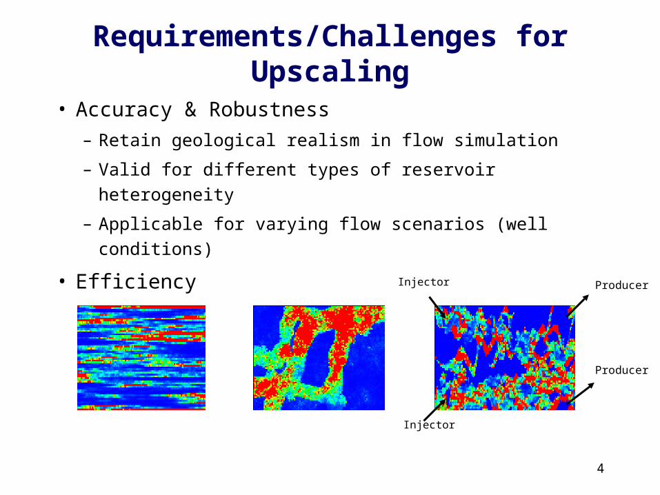
Reconstruction of Fine Scale Velocity

0 cp*k 0 )(

St

Sv

Upscaling, global

coarse scale flow

Solve local fine scale(kp)=0

Partition coarse

flux to fine scale

Reconstructed fine scale v

(downscaling)

• Readily performed in upscaling framework

12

Results: Performance of ALG

Averaged fine

Pressure Distribution

Coarse: extended local

Coarse: Adaptive local-global

Channelized layer (59) from 10th SPE CSP

Flow rate for specified

pressure

• Fine scale: Q = 20.86

• Extended T *: Q = 7.17

• ALG upscaling: Q = 20.010.0

5.0

10.0

15.0

20.0

25.0

0 1 2 3 4Iteration

Q

Q (Fine scale) = 20.86

ALG, Error: 4%

Extended local,

Error: 67%

Upscaling 220 60 22 6

13

Results: Multiple Channelized Layers

Extended local T * Adaptive local-global T *

10th SPE CSP

14

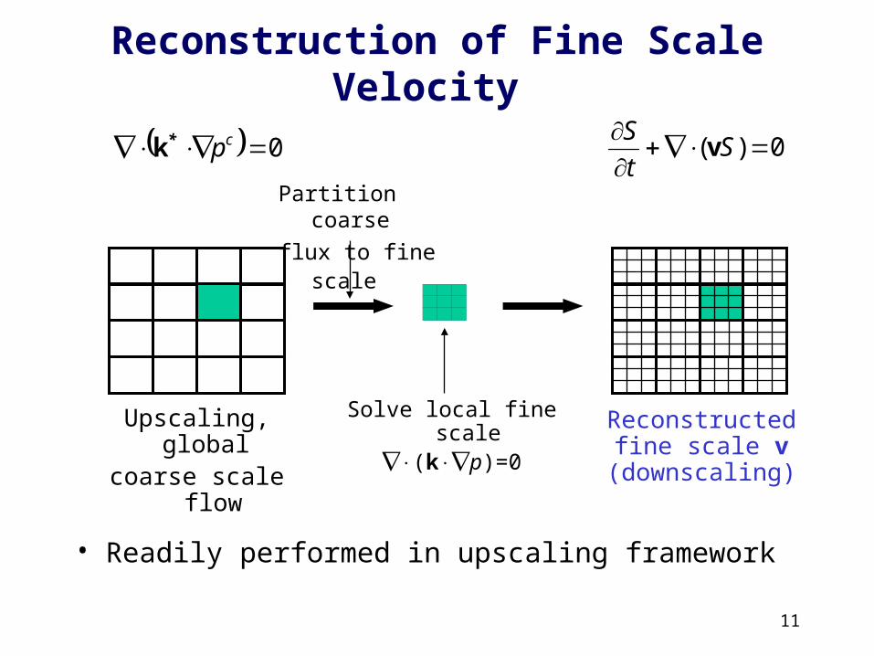
Another Channelized System

100 realizations 120 120 24 24

ALG T *T * + NWSU k * only

15

Results: Multiple Realizations

• 100 realizations conditioned to seismic and well data

• Oil-water flow, M=5

• Injector: injection rate constraint, Producer: bottom hole pressure constraint

• Upscaling: 100 100 10 10

100 realizations

Time (days)

BH

P (

PS

IA)

Fine scale

mean

90% conf. int.

16

Results: Multiple Realizations

Coarse: Purely local upscaling Coarse: Adaptive local-global

Time (days)

BH

P (

PS

IA)

Mean (coarse scale)

90% conf. int. (coarse scale)

Time (days) B

HP

(P

SIA

)

Mean (fine scale)

90% conf. int. (fine scale)

17

Results (Fo): Channelized System

220 60 22 6

Fractional Flow Curve

0

0.2

0.4

0.6

0.8

1

1.2

0 0.2 0.4 0.6 0.8 1PVI

Fo

Fine scale

ALG T *

Extended local T * Flow rates

• Fine scale: Q = 6.30

• Extended T *: Q = 1.17

• ALG upscaling: Q = 6.26

Oil cut from reconstruction

18

Results (Sw): Channelized System

Fine scale Sw (220 60)

Reconstructed Sw from

extended local T * (22 6)

0.5

1.0

0.0

Reconstructed Sw from

ALG T * (22 6)

Fine scale streamlines

19

Results for 3D Systems (SPE 10)

50 channelized layers, 3 wellspinj=1, pprod=0

Typical layers

Upscale from 6022050 124410

using different methods

20

Results for Well Flow Rates - 3D

Average errors

• k* only: 43%

• Extended T* + NWSU: 27%

• Adaptive local-global: 3.5%

21

Results for Transport (Multiscale) - 3D

fine scale

ALG T *

local T * w/nw

standard k*

Producer 1

Fo

PVI

fine scale

ALG T *

standard k*

Producer 2

local T * w/nwFo

PVI

• Quality of transport calculation depends on the accuracy of the upscaling

22

Velocity Reconstruction versus Subgrid Modeling

• Multiscale methods carry fine and coarse grid information over the entire simulation

• Subgrid modeling methods capture effects of fine grid velocity via upscaled transport functions:

- Pseudoization techniques

- Modeling of higher moments

- Generalized convection-diffusion model

23

• Coarse scale pressure and saturation equations of same form as fine scale equations

• Pseudo functions may vary in each block and may be directional (even for single set of krj in fine scale model)

Pseudo Relative Permeability Models

, 0),( ** cc pS kx 0),(

* c

c

StS

xF

)()(

)()(

),( ,=),(

**

*c*

c****

c*

oirowirw

wirwi

icii

o

ro

w

rw

μk+μkμk

Sf

SfFμkk

S

xvx

* upscaled function

c coarse scale p, S

24

Generalized Convection-Diffusion Subgrid Model for Two-Phase Flow

• Pseudo relative permeability description is convenient but incomplete, additional functionality required in general

• Generalized convection-diffusion model introduces new coarse scale terms

- Form derives from volume averaging and homogenization procedures

- Method is local, avoids need to approximate

- Shares some similarities with earlier stochastic approaches of Lenormand & coworkers (1998, 1999)

)()( yx ji vv

25

• Coarse scale saturation equation:

Generalized Convection-Diffusion Model

cccc

SSStS

),(),(

xDxG

),()(),( cccc SSfS xmvxG

• Coarse scale pressure equation:

cccc SSSWS ),(),()( 21* xWx

(modified convection m and diffusion D terms)

(modified form for total

mobility, Sc dependence)

“primitive” termGCD term

0),( ** cc pS kx

26

• D and W2 computed over purely local domain:

Calculation of GCD Functions

p = 1 S = 1

p = 0)()()( SfSfSS vvD

• m and W1 computed using extended local domain:

(D and W2 account for local subgrid effects)

SSSfSfS )()()( )( Dvvm

(m and W1 - subgrid effects due to longer range interactions)

target coarse block

27

Solution Procedure

• Generate fine model (100 100) of prescribed parameters

• Form uniform coarse grid (10 10) and compute k* and directional GCD functions for each coarse block

• Compute directional pseudo relative permeabilities via total mobility (Stone-type) method for each block

• Solve saturation equation using second order TVD scheme, first order method for simulations with pseudo krj

fine grid: lx lz

Lx = Lz

28

Oil Cuts for M =1 Simulations

• GCD and pseudo models agree closely with fine scale (pseudoization technique selected on this basis)

lx = 0.25, lz= 0.01, =2, side to side flow

100 x 100

10 x 10 (GCD)

10 x 10 (primitive)

10 x 10 (pseudo)

Oil

Cu

t

PVI

29

Results for Two-Point Geostatistics

x =0.05, y = 0.01, logk = 2.0

100x100 10x10, Side Flow

10

0

5

• Diffusive effects only

30

Results for Two-Point Geostatistics (Cont’d)

x =0.5, y = 0.05, logk = 2.0

100x100 10x10, Side Flow

10

0

5

• Permeability with longer correlation length

31

Effect of Varying Global BCs (M =1)

p = 1 S = 1

p = 0

0 t 0.8 PVI

p = 1 S = 1 t > 0.8 PVI

p = 0

lx = 0.25, lz= 0.01, =2

Oil

Cu

t

PVI

100 x 100

10 x 10 (GCD)

10 x 10 (primitive)

10 x 10 (pseudo)

lx = 0.25, lz= 0.01, =2

32

Corner to Corner Flow (M = 5)

100 x 100

10 x 10 (GCD)

10 x 10 (pseudo)

Oil

Cu

t

PVIT

ota

l Ra

tePVI

lx = 0.2, lz= 0.02, =1.5

• Pseudo model shows considerable error, GCD model provides comparable agreement as in side to side flow

33

Effect of Varying Global BCs (M = 5)

100 x 100

10 x 10 (GCD)

10 x 10 (pseudo)

Oil

Cu

t

PVIT

ota

l Ra

tePVI

lx = 0.2, lz= 0.02, =1.5

• Pseudo model overpredicts oil recovery, GCD model in close agreement

34

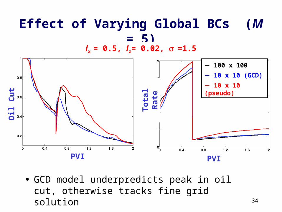
Effect of Varying Global BCs (M = 5)

lx = 0.5, lz= 0.02, =1.5

• GCD model underpredicts peak in oil cut, otherwise tracks fine grid solution

100 x 100

10 x 10 (GCD)

10 x 10 (pseudo)

Oil

Cu

t

PVIT

ota

l Ra

tePVI

35

),( * cc SS

0 ** cpkCoarse scale flow:

Pseudo functions:

GCD model:

T * from ALG, dependent on global flow

*, m(S c) and D(S c)

• Consistency between T * and * important for highly

heterogeneous systems

Combine GCD with ALG T* Upscaling

)( * cS

36

ALG + Subgrid Model for Transport (GCD)

t < 0.6 PVI t 0.6 PVI

• Stanford V model (layer 1)

• Upscaling: 100130 1013

• Transport solved on coarse scale

flow rate oil cut

37

flow simulation flow simulation

upscaling

gridding

diagnostic

GocadGocadinterface

coarse model

info. maps

fine model

Unstructured Modeling - Workflow

38

Numerical Discretization Technique

• CVFE method: – Locally conservative; flux on a face expressed as linear

combination of pressures

– Multiple point and two point flux approximations

• Different upscaling techniques for MPFA and TPFA

i j

k

qij = a pi + b pj + c pk + ... or qij = Tij ( pi - pj )

Primal and dual grids

39

3D Transmissibility Upscaling (TPFA)

Dual cells Primal grid connectionp=1

p=0fitted extended regions

cell j cell i

Tij*= -<qij>

<pj> <pi>-

40

Grid Generation: Parameters

• Specify flow-diagnostic

• Grid aspect ratio

• Grid resolution constraint:

– Information map (flow rate, tb)

– Pa and Pb , sa and sb

– N (number of nodes)

min max

1

property

cumulative frequency

a b

Pa

Pb

min max

Sa

Sb

property

resolution constraint

a b

41

velocity

grid density

Upscaled k*

Unstructured Gridding and Upscaling

(from Prevost, 2003)

42

Flow-Based Upscaling: Layered System

• Layered system: 200 x 100 x 50 cells

• Upscale permeability and transmissibility

• Run k*-MPFA and T*-TPFA for M=1

• Compute errors in Q/p and L1 norm of Fw

p=0p=1 1 0. 5

0.25

43

Flow-Based Upscaling: Results

0 0.2 0.4 0.6 0.8 10

0.2

0.4

0.6

0.8

1

PVI

Reference (fine)TPFAMPFA

8 x 8 x 18 = 1152 nodes 6 x 6 x 13 = 468 nodes

0 0.2 0.4 0.6 0.8 10

0.2

0.4

0.6

0.8

1

Fw

error in Fw error in Q/p

TPFA 7.6% -1.2%

MPFA 17.9% -25.2%

error in Fw error in Q/p

TPFA 16.8% -5.9%

MPFA 21.3% -31.7%

PVI

Fw

(from M. Prevost, 2003)

44

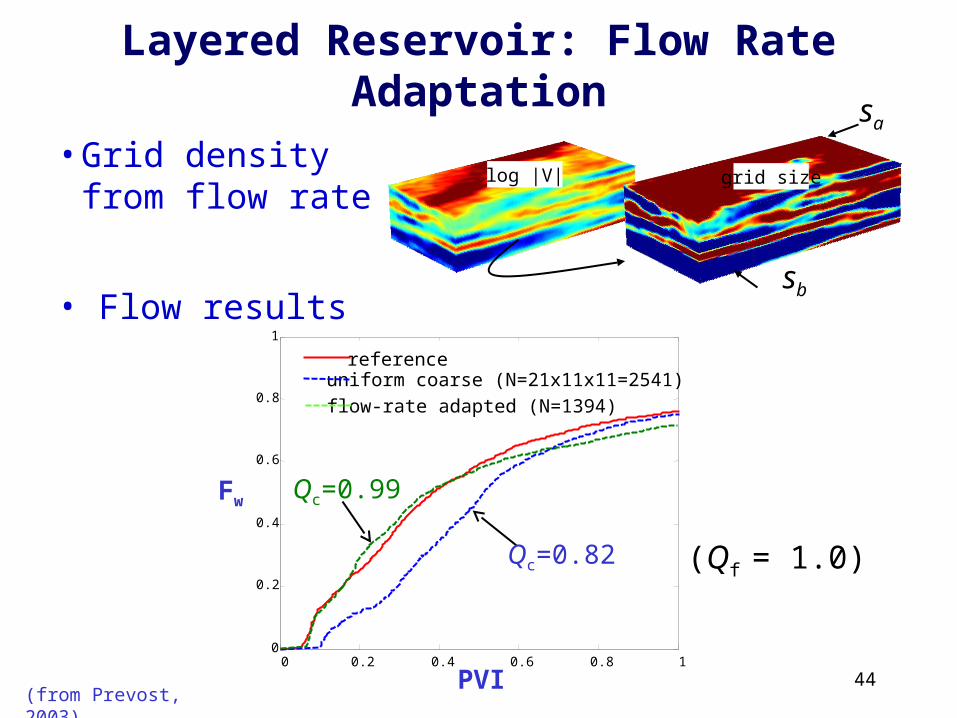
Layered Reservoir: Flow Rate Adaptation

• Grid density from flow rate

log |V| grid size

sb

sa

0 0.2 0.4 0.6 0.8 10

0.2

0.4

0.6

0.8

1

PVI

Fw

referenceuniform coarse (N=21x11x11=2541)

flow-rate adapted (N=1394)

Qc=0.82

Qc=0.99

PVI

Fw

• Flow results

(from Prevost, 2003)

(Qf = 1.0)

45

Summary

• Upscaling is required to generate realistic coarse scale models for reservoir simulation

• Described and applied a new adaptive local-global method for computing T *

• Illustrated use of ALG upscaling in conjunction with multiscale modeling

• Described GCD method for upscaling of transport

• Presented approaches for flow-based gridding and upscaling for 3D unstructured systems

46

Future Directions

• Hybridization of various upscaling techniques (e.g., flow-based gridding + ALG upscaling)

• Further development for 3D unstructured systems

• Linkage of single-phase gridding and upscaling approaches with two-phase upscaling methods

• Dynamic updating of grid and coarse properties

• Error modeling