Embed Size (px)
Citation preview

1/14
To appear in: Cement and Concrete Composites
(Special issue with papers from ICDC 2012)
June 2013
Updating of service-life prediction of reinforced concrete
structures with potential mapping
Sylvia Keßler1*, Johannes Fischer2, Daniel Straub2, Christoph Gehlen1
1Centre for Building Materials, Technische Universität München, Germany
2Engineering Risk Analysis Group, Technische Universität München, Germany
*Corresponding author: E-mail address: [email protected] (Sylvia Keßler)
Abstract
Fully probabilistic models are available for predicting the service life of new reinforced concrete
structures and for condition assessment of existing structures. Frequently, the decisive
mechanism limiting the service life of reinforced concrete structures is chloride-induced
corrosion, for which these models predict probabilistically the time to corrosion initiation. Once
the corrosion process is initiated, corroding areas can be detected nondestructively through
potential mapping. The spatial information gained from potential mapping can then be used for
updating the service-life prediction, taking into consideration the spatial variability of the
corrosion process. This paper introduces the spatial updating of the probabilistic model with
potential mapping and concrete cover measurements by means of Bayesian analysis. A case
study is presented, where potential mapping is applied prior to a destructive assessment, which
serves to verify the approach. It is found that the potential mapping can provide significant
information on the condition state. With the presented methods, this information can be
consistently included in the probabilistic service-life prediction.
Keywords: Life cycle prediction; potential mapping; updating; spatial variability.

2/14
1 Introduction
The fib Model Code for Service Life Design [1] provides methods for a fully probabilistic service-
life prediction for reinforced concrete (RC) structures subject to corrosion of the reinforcement.
For chloride-induced corrosion of the reinforcement, such methods facilitate the probabilistic
prediction of the time to corrosion initiation. The model code, however, does not address the
spatial variability of the occurrence of corrosion. Degradation of reinforced concrete structures
varies in space due to variation of geometry (e. g. concrete cover), concrete properties, (e. g.
chloride-migration), and exposure conditions (e. g. chloride impact). Local inaccuracies of the
construction process lead to additional spatial variability of corrosion. When planning
maintenance and repair activities, it is essential that this spatial variability is considered. In the
literature, several studies (Hergenröder [2], Faber et. al. [3], Malioka [4]) perform spatial
modeling of the corrosion initiation phase such as chloride ingress and carbonation through a
subdivision of the structure into elements. The element size is determined by the spatial
variability of the most important parameter of the corrosion initiation model. The spatial
variability of the corrosion propagation phase is considered e. g. in Li et al. [5], and Stewart and
Mullard [6].
Additional information on the beginning and extent of corrosion can be obtained through
condition assessments, e. g. by means of visual inspection and non-destructive testing such as
potential-field measurement. The inspection data not only provide information on the temporal
development of corrosion, but also enable an improved spatial description of corrosion. It is
possible to combine the results from these condition assessments with the probabilistic models
of corrosion through Bayesian updating. Using the data gained from inspection, Bayesian
updating is possible for single model parameters, for the deterioration model itself, and for the
deterioration probability. The incorporation of inspection data into the corrosion model by means
of Bayesian updating has demonstrated in the past [3,7-9]. A computationally efficient method
for updating the reliability with measurement data is proposed in [10].
This paper presents a procedure for Bayesian updating of the corrosion probability using
combined spatial data from both cover-depth and potential-field measurement on an existing
RC slab subject to chloride-induced corrosion of the reinforcement. The procedure is applied to
a case study, and the updated probabilistic predictions are compared to the actual conditions as
identified during the replacement of the concrete cover.
2 Methodology
2.1 Service-life prediction
The presentation hereafter is limited to chloride-induced corrosion of the reinforcement. In
concrete, embedded reinforcement is protected against corrosion due to the high alkalinity of
the pore solution. A thin iron oxide layer, the so called passive layer, is formed. The passive
layer can be destroyed locally by ingress of chlorides coming from deicing salt or seawater if a
critical chloride concentration is exceeded at the steel surface. This initiation period, i.e. the
probability of depassivation, can be calculated with a fully probabilistic model [1, 11]. The
corrosion process is initiated as soon as the concentration of chloride ions (equation (1))
exceeds a certain critical concentration at the level of the reinforcement.
A diffusion model is applied to estimate the chloride concentration at the level of the
reinforcement. With given surface concentration and diffusion coefficient , the concentration
of chloride ions at time in depth is given by

3/14
( ) ( (
√ )) (1)
In this equation, is assumed to be constant. However, this is not the case in reality [1,11]. To
adapt the diffusion model to the actual environmental onsite conditions, to specific concrete
properties, and to account for its time-dependency, the diffusion coefficient in equation (2) is
modified following [1,11] to
( ) (
) . (2)
The chloride- ng ss mod l s bas d on a solu on of F k’s s ond law of d ffus on assum ng
ha d ffus on s h dom nan anspo m han sm. How v , F k’s d ffus on law s no suitable
for describing the transport mechanisms in the near-surface layer, since it assumes a stationary
surface concentration of chloride ions in time. In reality, due to intermittent wetting and drying,
the surface concentration and varies with time. For that reason, the diffusion is modeled only
beyond the depth of a convection layer , where a substitute surface concentration of is
applied. Modifying equation (1) accordingly and inserting the time-dependent diffusion
coefficient of equation (2), one obtains
( )
(
(
√ ( )
)
)
(3)
with the deterioration model parameters:
Critical corrosion inducing chloride content at depth of reinforcement [wt.-%/cem.],
Substitute surface chloride concentration at depth [wt.-%/cem.],
Concrete cover depth [mm],
Thickness of the convection zone layer [mm],
Rapid chloride migration coefficient [mm²/a],
Factor for considering temperature impact on [-],
Transfer parameter (test method) [-],
Reference testing time ( d) [a],
Aging exponent [-].
The dimensionless correction factor accounts for the influence of the actual onsite
temperature and is given by
( (
f
al
)) , (4)
where al is the onsite temperature, f is the reference temperature, and is a regression
parameter (all in [K]) [1,11].
Finally, the event of corrosion at time is written as

4/14
{
(
(
√ ( )
)
)
}
(5)
Most of the parameters in equation (5) are modeled as random variables. In the case study
presented later, specific probability distribution models for these parameters are presented.
Let now [ ] be h v o of h mod l’s bas andom
variables with their joint PDF ( ), and denotes the domain in the outcome space of
corresponding to the event . The corrosion probability is then given by
( ) ∫ ( )
(6)
wherein ∫ denotes the integration over the failure domain . This integral can be
evaluated using any structural reliability method (SRM), such as FORM or Monte-Carlo
methods [12,13].
2.1.1 Random field modeling of corrosion
Some of the model parameters vary randomly in space. As an example, consider the concrete
cover depth at a certain location A. With high probability, the cover depth at a neighboring
location will have a value similar to the one in A, whereas the cover depth at a faraway location
is likely to be independent of the one in A. To account for such spatial correlation of model
parameters, they are modeled as spatial random fields. Random field modeling of corrosion in
RC structures has been presented in several studies; e.g. [3,14,15]. Using a second-order
description of the random field, it is necessary to specify the spatial covariance matrix in
addition to the marginal probability distributions.
In the case study presented later, all spatially varying parameters are described by
homogenous, isotropic random fields. The spatial covariance matrix of any random variable is
described by a monotonically decreasing function:
[ ] [ ] (
) , (7)
with
Distance between location and [m],
Correlation length of the random variable [m],
Standard deviation of the random variable [Unit of the variable itself].

5/14
2.2 Updating the service-life prediction
2.2.1 Bayesian updating
When measurement data from inspection or monitoring are available, these can be directly
used for updating the probability of corrosion. The model updating after an inspection is
straightforward by apply ng Bay s’ ul :
( ond on nsp on) ( nsp on ond on) ( ond on) , (8)
where is a normalizing constant ensuring that the sum or the integral over all possible
conditions results in one. ( ond on) represents the prior knowledge on the structural
condition coming from the a-priori service-life prediction. ( nsp on ond on) is the
likelihood of the observed inspection result for a given condition. Finally,
( ond on nsp on) is the a-posteriori probability of a specific condition given the
inspection result. A detailed description of the implementation of the Bayesian updating
procedure is presented in [10,14,15].
For updating, three different types of measurements are potentially available: The first type are
measurements of a direct model parameter of the deterioration model; in the case study, we
use onsite measured data of the cover depth . The second type includes direct or indirect
measurements of the condition state; in the case study we use measurement data from
potential mapping. The third type is given by measuring quantities that are related to the
condition state through the deterioration model, e. g. measurements of the chloride
concentration at certain depths (see e.g. [14, 15]). The updating with the measurements
available in the case study is described in the following two sections.
2.2.2 Updating with data from cover depth measurement
Since the cover depth is a direct model parameter in equation (5), we may update the
corrosion probability by updating only the probability density function (PDF) of the cover depth,
( ), and then use the posterior PDF
( ) in the probabilistic calculation. Since the cover
depth is modeled as a discretized random field, the updating must be performed on the joint
PDF of the cover depth at all discrete locations on the surface.
Using the measurement data m [ m m m ] , the mean value and the covariance
matrix (introduced in equation (7)) of the cover depth are updated following the procedure
described in [14]. The posterior corrosion probability is estimated using (6), by replacing ( )
with its posterior
( ).
2.2.3 Updating with data from potential mapping
An effective inspection method is the potential mapping, which is able to indicate corroding
(active) and noncorroding (passive) areas in RC structures [16]. Therefore, potential mapping
data is used to check if and where corrosion has started. Potential mapping yields information
about the corrosion condition state at the time of the measurement; direct statements about
corrosion processes in the past or future are not possible. The advantage of potential mapping
is that measurements can be performed in a grid over the whole structure or a component, and,
in this way, potential mapping delivers spatial information on the corrosion condition state.

6/14
During potential mapping, the potential difference m between an external reference electrode
and the reinforcement is measured. A lower potential indicates a higher probability of corrosion.
Exemplarily, Figure 1 shows the potential differences measured on the RC element considered
in the case study. The data is summarized in a histogram of 50 equally spaced intervals of width
mV.
Figure 1: The histogram of the measured potential differences.
To perform the probability updating with the potential mapping m, the domains where the
reinforcement is either active or passive should be distinguished. Since it is not possible to
deterministically identify a threshold potential, a probabilistic approach is pursued as described
in the following.
Commonly, the potential differences in the active and the passive areas are modeled as
normally distributed [17]. Using the Maximum Likelihood Estimate (MLE) method for parameter
estimation [18,19], it is possible to find the two normal distributions that fit the data most
suitable. This is illustrated in Figure 2: The black curve denotes the PDF of the potential
difference given the reinforcement is active, , and the black dashed curve shows the PDF of
the potential difference given the reinforcement is passive, ̅. The gray curve represents the
combined PDF of the potential differences, ( ).
Figure 2: The density functions of the potential difference for active (black) and passive (black dashed)
reinforcement, as well as their combined PDF (gray).
In Figure 3, the cumulative density function (CDF) of the fitted combined distribution is
compared to the empirical CDF, which corresponds to the histogram of Figure 1. The figure
indicates a good fit between potential measurement and the combined distribution estimated by
MLE.
-500 -400 -300 -200 -100 00
20
40
60
80
100
Potential difference [mV]
Mea
sur
emen
t cou
nt

7/14
Figure 3: The analytical CDF of the measured potential differences m estimated by MLE agrees with the
empirical CDF.
From Figure 2 it can be observed that - for the examined structure - potentials lower than
mV are likely to be associated with corroding reinforcement. For potential values larger
than mV, the corrosion probability decreases with increasing potentials. As can be
recognized in Figure 2, there is a large domain where the active and the passive distribution
overlap. In this domain, the likelihood of planning the wrong measures is higher: either a repair
is executed although it is not necessary, or a wrong all-clear may result in further damage and
additional costs in the future.
To calculate the updated depassivation probability, ( m), the rule for conditional
probabilities depicted in equation (8) is applied for each element on the concrete surface.
Using the density function for the active corrosion, ( ), as estimated earlier, the
probability updating becomes
( m) ( ) ( )
( ) ( ) ̅( ̅) ( ̅) (9)
3 Numerical investigation
3.1 Case study
The case study is a reinforced concrete underpass in a city with increasing traffic volume,
shown in Figure 4. Due to the climate and the traffic situation, the structure belongs to the
exposure class XD3 following EN 206-1 [20], which is characterized by cyclic wetting and drying
in combination with severe chloride impact. The underpass was built in 1961. The inspection
data were generated in 2008 when the structure was 47 years old. The underpass consists of
abutments and retaining walls. Each side of the underpass is longer than 200 m. For a better
overview, only the evaluation of one section of the retaining wall is presented (field 14, as
indicated in Figure 4).
-500 -400 -300 -200 -100 00
0.2
0.4
0.6
0.8
1
Potential difference [mV]
CD
F o
f pot
entia
l diff
eren
ceEmpirical CDF
(observed potentials)
Analytical CDF

8/14
Figure 4: Underpass with the selected section of the retaining wall: field 14 (marked) [Source: GoogleEarth].
3.2 Probabilistic model
Due to the age of the structure, information on the concrete composition and properties is not
available. Considering the materials and codes commonly used during time of construction, it is
assumed that a Portland cement with a water/binder ratio of 0.5 was used. The probabilistic
service-life prediction is calculated using the input parameters of Table 1, which were obtained
for the specific material and environmental conditions from [1]. For the spatial modeling, the
correlation length of all spatially varying parameters is assumed to be . m.
The prior corrosion probability computed with Monte-Carlo simulation (MCS) is shown in Figure
5. The calculation is based on data of Table 1. Since no spatial information is available a-priori,
the corrosion probability is equal for each element on the whole surface. At the time of the
inspection, in year 47, the probability of co os on n a on s 6 %.
Figure 5: Prior corrosion probability of the reinforcement calculated with MCS.

9/14
Table 1: The random model input parameters, their distributions, and distribution parameters for the full
probabilistic corrosion initiation model following the fib bulletin [1], further data from [11].
Parameter Unit Distribution
[10-12
m²/s] Normal 498.3 99.7 2.0
[-] Beta 0.3 0.12
[a] - 0.0767
nsp [a] - 47
[-] - 1 - -
f [K] - 293 -
al [K] Normal 282 3 -
[K] Normal 4800 700 -
s [wt.%/cem.] Lognormal 2.73 1.23 2.0
[wt.%/cem.] Beta 0.6 0.15
[mm] Beta 8.9 5.6 2.0
[mm] Lognormal 40 13 2.0
3.3 Inspection data
Concrete cover measurements and potential mapping were performed on the entire surface.
The measurement grid was chosen as . m . m in and direction, respectively. The
following illustrations in Figure 6 show the inspection data obtained from field 14. The histogram
of measured potential differences is given in Figure 1.
10/14
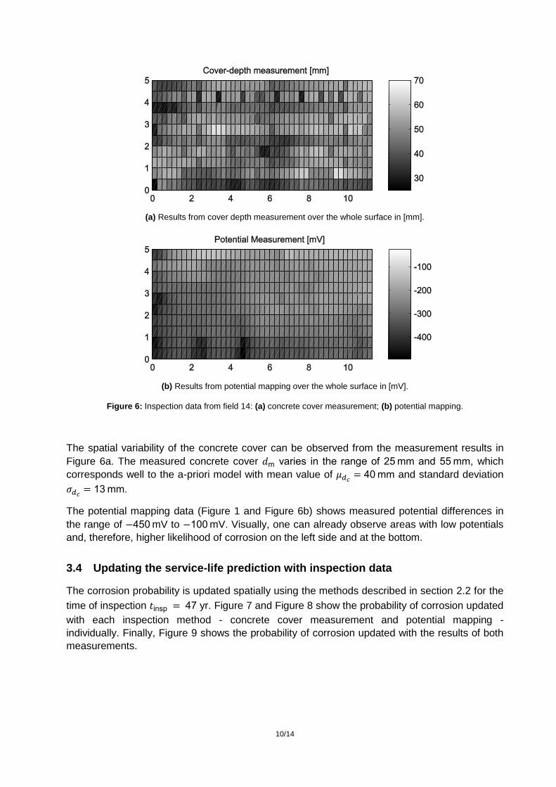
(a) Results from cover depth measurement over the whole surface in [mm].
(b) Results from potential mapping over the whole surface in [mV].
Figure 6: Inspection data from field 14: (a) concrete cover measurement; (b) potential mapping.
The spatial variability of the concrete cover can be observed from the measurement results in
Figure 6a. The measured concrete cover m va s n h ang of mm and mm, which
corresponds well to the a-priori model with mean value of mm and standard deviation
mm.
The potential mapping data (Figure 1 and Figure 6b) shows measured potential differences in
the range of mV to mV. Visually, one can already observe areas with low potentials
and, therefore, higher likelihood of corrosion on the left side and at the bottom.
3.4 Updating the service-life prediction with inspection data
The corrosion probability is updated spatially using the methods described in section 2.2 for the
time of inspection nsp yr. Figure 7 and Figure 8 show the probability of corrosion updated
with each inspection method - concrete cover measurement and potential mapping -
individually. Finally, Figure 9 shows the probability of corrosion updated with the results of both
measurements.

11/14
Figure 7: Updated corrosion probability on the scale from 0.1 to 0.9 over the whole surface of field 14 using
data from cover depth measurement.
Figure 8: Updated corrosion probability over the whole surface of field 14 using potential mapping data.
Figure 9: Updated corrosion probability over the whole surface of field 14 using data from both cover depth
measurement and potential mapping.
The model updated with cover depth measurements (Figure 7) shows corrosion probabilities
between 20 % and 6 %. Major parts of the area have a corrosion probability of 20 %. Two
spots with higher corrosion probabilities are in the left side above and in the middle below.
The corrosion probability after updating with potential mapping data (Figure 8) indicates a
division of the inspected field diagonal into two parts. The left side and the lower parts have high
corrosion probabilities with values of over 90 %. Along the boundary to the top right side,
corrosion probabilities of approximately 60 % down to 0 % are calculated.

12/14
The updating with potential mapping and the updating with cover depth give different results.
The concrete cover measurements cannot directly predict the deterioration condition and its
interpretation depends on the model. In particular, the model does not take into account the
actual spatial distribution of the chloride impact and singularities in the structure, such as the
joint on the left side of field 14, where chloride-contaminated water from the road above could
flow off. With advanced age of the structure, potential mapping indirectly reflects the spatial
distribution of the chloride impact. This is the case above, where the zone with chloride-
contaminated water is clearly identifiable.
The combined updating of the corrosion probability using data from both cover depth
measurement and potential mapping (Figure 9) indicates similar results as the update using
only potential mapping data. In the case of a structure with significant active corrosion, the
potential mapping appears to provide more information than the more indirect cover depth
measurement.
It is noted that the corrosion probability is high in general. This is explained partly by the fact
that the structure is relatively old and exposed to one of the most aggressive exposure
conditions, as already reflected in the prior probability.
3.5 Comparison of the updated corrosion probabilities to the real condition
Following the inspection results, the structure was repaired. The outer concrete cover was
replaced until behind the first reinforcement layer. Therefore, the corrosion condition of the
reinforcement was visible in the form of loss of cross section. Figure 10 shows the loss of cross
section map.
Figure 10: Loss of cross section (marked) identified through visual inspection.
The observed corrosion condition ranges from superficial corrosion with a roughened surface to
complete loss of cross section. With visual inspection, one cannot indicate all corroding areas,
because the reinforcement exhibits no loss of cross section where corrosion has just started.
Comparing the updated corrosion probability (Figure 9) to the real condition (Figure 10), a larger
corroding area was predicted than revealed by the visual inspection.
This result can be explained in two ways. Firstly, as stated above, visual inspection is not able
to identify all corroding areas. Secondly, an electrochemical effect takes place that is not
accounted for in the model: The reinforcement surface around a corroding area automatically
behaves as a cathode. So this surrounding area is thus naturally protected against corrosion.
The expansion of the resulting potential field due to an anode can reach more than one meter
[21]. Consequently, low potentials are measured at the concrete surface, although the

13/14
reinforcement under the concrete surface is a cathode. This explains the non-corroding areas
in-between the corroding ones.
The corrosion-probability updating has identified all corroding areas; no anode area was
overlooked. However, also some non-corroding areas were indicated as corroding. Therefore,
the updating criterion for the potential mapping data appears to be conservative. Additional
research is needed to identify a more differentiated criterion for updating the service life
prediction with potential mapping.
4 Summary and outlook
Maintaining the serviceability of aging reinforced concrete structures is a major task in
infrastructure management. Probabilistic service-life prediction with additional consideration of
inspection data is a powerful tool to support this task. This paper presents a case study of an
updating of the service-life prediction of a concrete structure with concrete-cover measurements
and potential-mapping data. The special innovation of this procedure is the consideration of the
spatial variability of the deterioration process. Inspection and maintenance planning can be
executed more precisely by taking into account the spatial variability of the deterioration
process. As a result, this approach enables the reduction of maintenance costs over the life
cycle of structures.
The presented case study indicates that the potential mapping provides more information on the
corrosion probability for structures in which corrosion has already initiated. Concrete-cover
measurements exhibit the advantage of being time-independent. Therefore, they can be applied
already at an early stage before corrosion starts. As shown by the visual inspection of the
reinforcement, the computed posterior probabilities correspond well to the actual corrosion state
of the structure.
The next step to complete the presented framework is the implementation of the corrosion
propagation model, which will enable the prediction of the probability of cross section loss of the
steel reinforcement, and therefore allows predicting the reliability of concrete structures.
Acknowledgment
The authors wish to thank the engineering consultancy Ingenieurbüro Schießl Gehlen Sodeikat
GmbH and the Munich administration for supporting the project by providing the measurement
data.
5 References
1. Schießl P, Bamforth P, Baroghel-Bouny, V, Corley G, Faber M, Forbes J, Gehlen C, et al.
Model code for service life design. fib bulletin 34, 2006
2. Hergenröder M. (1992). Zur Statistischen Instandhaltungsplanung für bestehende
Bauwerke bei Karbonatisierung des Betons und möglicher Korrosion der Bewehrung.
Berichte aus dem Konstruktiven Ingenieurbau 4/92, TU München. (German)
3. Faber MH, Straub D, Maes MA. A Computational Framework for Risk Assessment of RC
Structures Using Indicators, Computer-Aided Civil and Infrastructure Engineering 21, 2006
216-230.

14/14
4. Malioka V. Condition Indicators for the Assessment of Local and Spatial Deterioration of
Concrete Structures, Diss ETH No. 18333, 2009.
5. Li Y, Vrouwenvelder T, Wijnants GH, Walraven J (2004). Spatial variability of concrete
deterioration and repair strategies. Structural Concrete, 5(3): 121–129.
6. Stewart MG, Mullard JA (2007). Spatial time-dependent reliability analysis of corrosion
damage and the timing of first repair for RC structures, Engineering Structures, 29(7),
1457–1464.
7. Maes MA (2002). Updating performance and reliability of concrete structures using discrete
empirical Bayes methods. Journal of Offshore Mechanics and Arctic Engineering, ASME,
124(4): 239–246.
8. Straub D., Malioka V., Faber M.H. (2009). A framework for the asset integrity management
of large deteriorating concrete structures. Structure and Infrastructure Engineering, 5(3) pp.
199 - 213.
9. Schoefs F, Tran TV, Bastidas-Arteaga E. Optimization of inspection and monitoring of
structures in case of spatial fields of deterioration properties, Proceeding ICASP, Zürich
2011
10. Straub D. Reliability updating with equality information. Probabilistic Engineering
Mechanics, 26(2), 254-258, 2011
11. Gehlen C. Probabilistische Lebensdauerbemessung von Stahlbetonbauwerken:
Zuverlässigkeitsbetrachtungen zur wirksamen Vermeidung von Bewehrungskorrosion.
Berlin: Beuth, 2000 (Deutscher Ausschuss für Stahlbeton 510). – ISBN 978-3-410-65710-1,
2000 (German).
12. Ditlevsen O. Uncertainty modeling with applications to multidimensional civil engineering
systems. New York McGraw-Hill, 1981. – ISBN 0-07-017046-0
13. Ditlevsen O, Madsen HO. Structural reliability methods. Chichester: Wiley, 1996. – ISBN 0
471 96086 1
14. Fischer J, Straub D. Reliability Assessment of Corroding Reinforced Concrete Slabs with
inspection Data. In: 9th Int. Probabilistic Workshop Braunschweig, 2011
15. Straub D. Spatial reliability assessment of deteriorating reinforced concrete surfaces with
inspection data. Proc. ICASP 2011, Zürich, 2011
16. Menzel K, Preusker H. Potentialmessung: Eine Methode zur zerstörungsfreien Feststellung
von Korrosion an der Bewehrung. Bauingenieur 64, 181-186, 1989 (German)
17. Elsener B, Böhni H. Electrochemical methods for the inspection of reinforcement corrosion.
Concrete structures-field experience. Material Science Forum, 1992:635-646.
18. Lindley DV. Introduction to Probability & Statistics. Cambridge University Press, 1965
19. Benjamin JR, Cornell CA. Probability, Statistics and Decision for Civil Engineers. McGraw-
Hill Book Company, New York, USA, 1970.
20. EN 206-1/ DIN 1045-2
21. Keßler S, Gehlen C. Potential mapping - Possibilities and limits. In: 8th fib PhD Symposium
20-23 June 2010 in Lyngby, Denmark.