A BLIND PREDICTION TEST OF NONLINEAR ANALYSIS …3)0142.pdf · 142 A BLIND PREDICTION TEST OF NONLINEAR ANALYSIS PROCEDURES FOR REINFORCED CONCRETE SHEAR WALLS Trevor Kelly1 ABSTRACT

142

A BLIND PREDICTION TEST OF NONLINEAR ANALYSIS PROCEDURES FOR REINFORCED CONCRETE SHEAR WALLS

Trevor Kelly1

ABSTRACT

A full scale slice of a 7 story reinforced concrete building was tested on the shake table at the UCSD Engelkirk Structural Research Centre in 2006. As part of the research project, a blind prediction contest was sponsored to assess the capability of currently available analysis procedures to predict the seismic response of cantilever reinforced concrete shear wall structures. This paper describes an entry based on a nonlinear finite element model, using macro elements to represent both the shear and the flexural modes of behaviour. A comparison of the predicted response with the test results showed that the analysis procedure produced reasonable predictions of deformations for the lowest and highest of the four earthquakes but under-estimated response for the two moderate earthquakes by approximately 30%. For all earthquakes, the analysis base moment was much lower than the test value. Modifications to the procedure to improve the correlation were identified and implemented but did not remedy the deficit in base moments. Detailed results of the test program revealed that the causes for this discrepancy were the contribution to overturning results of gravity columns and the flange wall, neither of which had been included in the model. When these were incorporated the average error between test and analysis results was less than 10% for all earthquakes, well within acceptable limits for a design office type of model. The correlation of tests and analysis also provided useful information on design aspects for shear walls, such as the influence of secondary components and dynamic magnification factors. Keywords: Reinforced concrete shear walls, reinforced concrete, nonlinear analysis, capacity curve, pushover analysis, hysteresis, earthquake, performance based design.

1 INTRODUCTION

A full scale slice of a 7 story reinforced concrete building was tested by the University of California at San Diego (UCSD) at the unidirectional NEES-UCSD Large High Performance Outdoor Shake Table at the Englekirk Structural Research Centre in 2006. The test program, which included various low intensity white noise tests plus a low intensity earthquake motion, two medium intensity earthquakes and a large intensity earthquake, is described by Panagiotou et al [2006a]. A blind prediction contest sponsored by UCSD, the Portland Cement Association and the Network for Earthquake Engineering Simulation (NEESinc) invited participants to predict the response of the test wall to the four input earthquake motions. This paper describes an entry based on a nonlinear finite element model, using macro elements to represent both the shear and the flexural modes of behaviour as described in a previous paper by Kelly [2004]. A comparison of the predicted response with the test results showed that the analysis procedure produced reasonable displacement results, within 8%, for the lowest and highest of the four earthquakes but under-estimated the response for the two moderate earthquakes by approximately 30%. For all earthquakes, the analysis base moment was much lower than

the test value, with the discrepancy increasing from 12% at EQ1 to 45% at EQ4. A number of relatively minor modifications to the analysis procedure were identified and implemented. These improved the displacement and acceleration correlations but the discrepancy between test and analysis base moments remained. In late 2006 the results were presented at a workshop held at UCSD for all participants [Kelly, 2006]. Presentations at this workshop by the test personnel revealed that two construction aspects which had been ignored by most contest participants significantly influenced the results [Panagiotou and Restrepo, 2006b]. These were the gravity columns and the flange walls, which were not intended to be part of the lateral load system but in fact contributed significantly to the overturning resistance of the web wall. The effects of the gravity column and flange wall were incorporated into the model and this improved the correlation to the extent where the average error of all response quantities was within ±10%, which is well within expectations for the type or macro model used. This paper identifies improvements to analysis procedures for shear wall structures as a result of this test program and also discusses general aspects of the seismic response of shear wall structures. This influence of elements which are

1 Partner, Holmes Consulting Group, Auckland (Member)

BULLETIN OF THE NEW ZEALAND SOCIETY FOR EARTHQUAKE ENGINEERING, Vol. 40, No. 3, September 2007

143

not considered to be part of the structural system, and methods by which they may be incorporated into the analysis procedures, is also discussed.

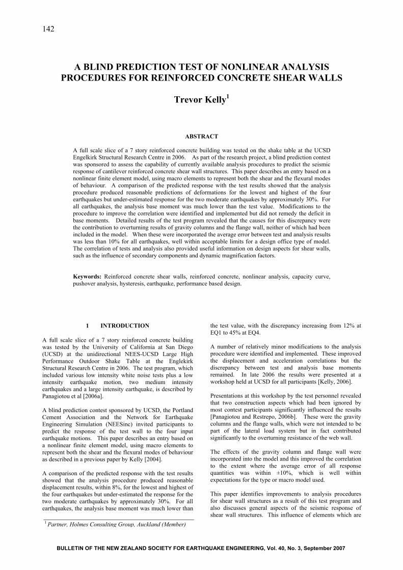
2 UCSD TEST STRUCTURE The test structure was a full scale slice of a 7-story residential building incorporating structural walls as the lateral force-resisting system. The test comprised a 3.658 m long web wall 19.202 high which provided lateral force resistance in the E-W direction of loading, as shown in the Elevation in Figure 1.

Web Wall

FlangeWall

Post tensionedprecastsegmental pier

Horizontalsteel truss

7 @

2.7

43 m

= 1

9.20

2 m

3.658 m

Slotsin Slab

Concrete slabs203 mm (L1,L7)152 mm (L2-L6)

Figure 1. Elevation of Test Specimen

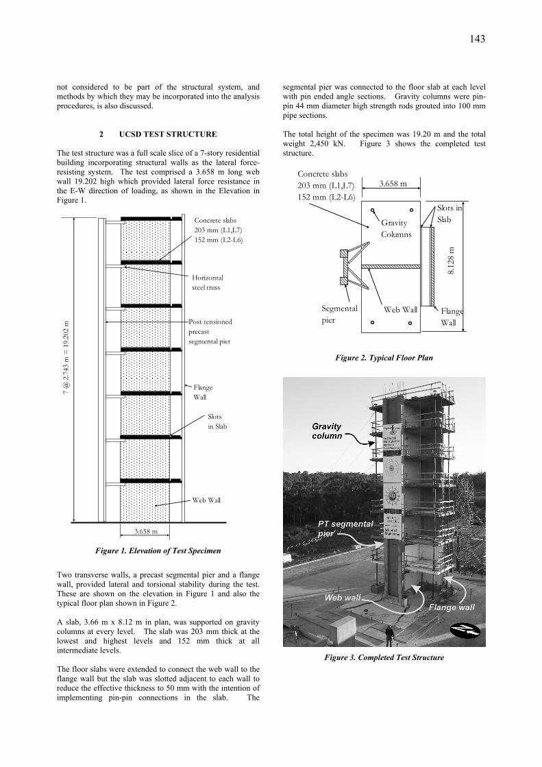
Two transverse walls, a precast segmental pier and a flange wall, provided lateral and torsional stability during the test. These are shown on the elevation in Figure 1 and also the typical floor plan shown in Figure 2. A slab, 3.66 m x 8.12 m in plan, was supported on gravity columns at every level. The slab was 203 mm thick at the lowest and highest levels and 152 mm thick at all intermediate levels. The floor slabs were extended to connect the web wall to the flange wall but the slab was slotted adjacent to each wall to reduce the effective thickness to 50 mm with the intention of implementing pin-pin connections in the slab. The

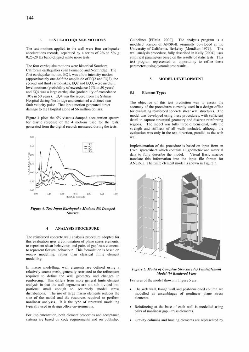
segmental pier was connected to the floor slab at each level with pin ended angle sections. Gravity columns were pin-pin 44 mm diameter high strength rods grouted into 100 mm pipe sections. The total height of the specimen was 19.20 m and the total weight 2,450 kN. Figure 3 shows the completed test structure.

GravityColumns

Segmentalpier

Web Wall

3.658 m

FlangeWall

8.12

8 m

Concrete slabs203 mm (L1,L7)152 mm (L2-L6)

Slots inSlab

Figure 2. Typical Floor Plan

Figure 3. Completed Test Structure

144

3 TEST EARTHQUAKE MOTIONS

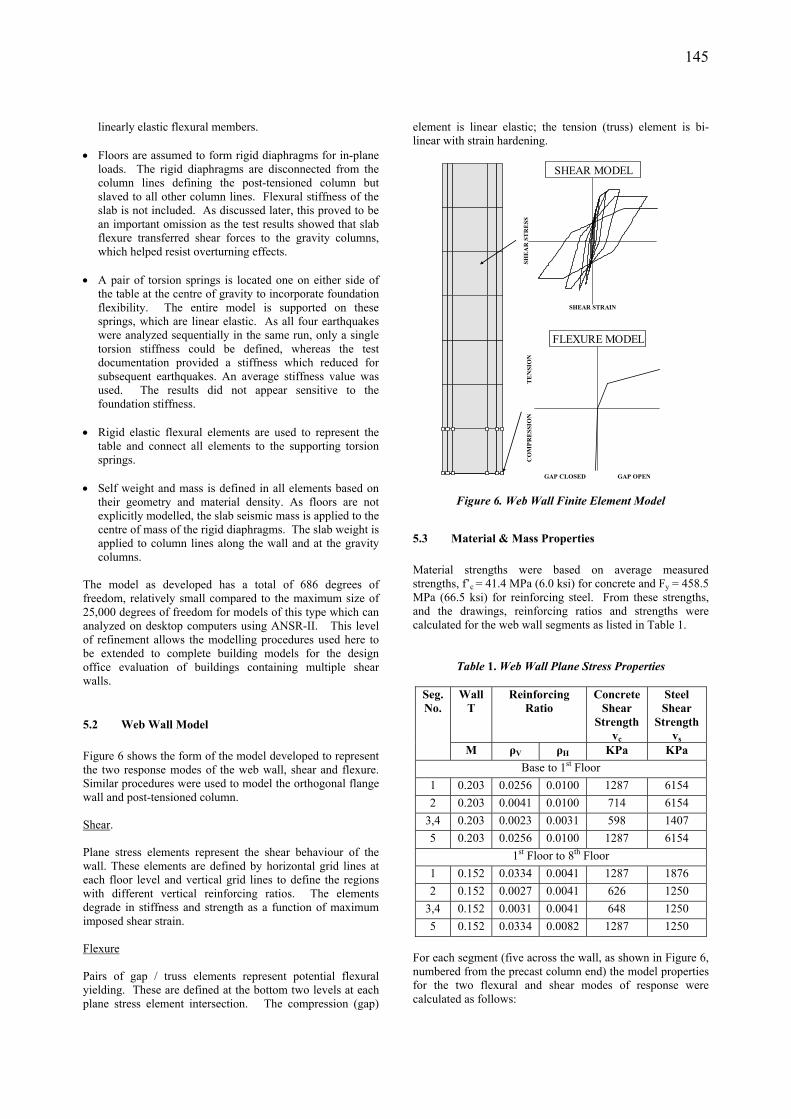
The test motions applied to the wall were four earthquake accelerations records, separated by a series of 2% to 5% g 0.25-20 Hz band-clipped white noise tests. The four earthquake motions were historical Southern California earthquakes (San Fernando and Northridge). The first earthquake motion, EQ1, was a low intensity motion (approximately one-half the amplitude of EQ2 and EQ3), the second and third earthquakes, EQ2 and EQ3, were medium level motions (probability of exceedance 50% in 50 years) and EQ4 was a large earthquake (probability of exceedance 10% in 50 years). EQ4 was the record from the Sylmar Hospital during Northridge and contained a distinct near-fault velocity pulse. That input motion generated direct damage to the Hospital alone of $6 million dollars. Figure 4 plots the 5% viscous damped acceleration spectra for elastic response of the 4 motions used for the tests, generated from the digital records measured during the tests.

0.00

0.50

1.00

1.50

2.00

2.50

3.00

0.00 0.25 0.50 0.75 1.00 1.25 1.50PERIOD (Seconds)

ACC

ELE

RATI

ON

(g)

EQ1EQ2EQ3EQ4

Figure 4. Test Input Earthquake Motions 5% Damped Spectra

4 ANALYSIS PROCEDURE The reinforced concrete wall analysis procedure adopted for this evaluation uses a combination of plane stress elements, to represent shear behaviour, and pairs of gap/truss elements to represent flexural behaviour. This formulation is based on macro modelling, rather than classical finite element modelling. In macro modelling, wall elements are defined using a relatively coarse mesh, generally restricted to the refinement required to define the wall geometry and changes in reinforcing. This differs from more general finite element analysis in that the wall segments are not sub-divided into portions small enough to accurately model stress distributions. The use of large macro elements reduces the size of the model and the resources required to perform nonlinear analyses. It is the type of structural modelling typically used in design office environments. For implementation, both element properties and acceptance criteria are based on code requirements and on published

Guidelines [FEMA, 2000]. The analysis program is a modified version of ANSR-II, originally developed at the University of California, Berkeley [Mondkar, 1979]. The wall analysis procedure, fully described in Kelly [2004], uses empirical parameters based on the results of static tests. This test program represented an opportunity to refine these parameters using dynamic test results.

5 MODEL DEVELOPMENT

5.1 Element Types The objective of this test prediction was to assess the accuracy of the procedures currently used in a design office for evaluating reinforced concrete shear wall structures. The model was developed using these procedures, with sufficient detail to capture structural geometry and discrete reinforcing regions. The model was fully three dimensional, with the strength and stiffness of all walls included, although the evaluation was only in the test direction, parallel to the web wall. Implementation of the procedure is based on input from an Excel spreadsheet which contains all geometric and material data to fully describe the model. Visual Basic macros translate this information into the input file format for ANSR-II. The finite element model is shown in Figure 5.

Figure 5. Model of Complete Structure (a) FiniteElement Model (b) Rendered View

Features of the model shown in Figure 5 are: • The web wall, flange wall and post-tensioned column are

modelled as assemblages of nonlinear plane stress elements.

• Reinforcing at the base of each wall is modelled using

pairs of nonlinear gap – truss elements. • Gravity columns and bracing elements are represented by

145

linearly elastic flexural members. • Floors are assumed to form rigid diaphragms for in-plane

loads. The rigid diaphragms are disconnected from the column lines defining the post-tensioned column but slaved to all other column lines. Flexural stiffness of the slab is not included. As discussed later, this proved to be an important omission as the test results showed that slab flexure transferred shear forces to the gravity columns, which helped resist overturning effects.

• A pair of torsion springs is located one on either side of

the table at the centre of gravity to incorporate foundation flexibility. The entire model is supported on these springs, which are linear elastic. As all four earthquakes were analyzed sequentially in the same run, only a single torsion stiffness could be defined, whereas the test documentation provided a stiffness which reduced for subsequent earthquakes. An average stiffness value was used. The results did not appear sensitive to the foundation stiffness.

• Rigid elastic flexural elements are used to represent the

table and connect all elements to the supporting torsion springs.

• Self weight and mass is defined in all elements based on

their geometry and material density. As floors are not explicitly modelled, the slab seismic mass is applied to the centre of mass of the rigid diaphragms. The slab weight is applied to column lines along the wall and at the gravity columns.

The model as developed has a total of 686 degrees of freedom, relatively small compared to the maximum size of 25,000 degrees of freedom for models of this type which can analyzed on desktop computers using ANSR-II. This level of refinement allows the modelling procedures used here to be extended to complete building models for the design office evaluation of buildings containing multiple shear walls.

5.2 Web Wall Model Figure 6 shows the form of the model developed to represent the two response modes of the web wall, shear and flexure. Similar procedures were used to model the orthogonal flange wall and post-tensioned column. Shear. Plane stress elements represent the shear behaviour of the wall. These elements are defined by horizontal grid lines at each floor level and vertical grid lines to define the regions with different vertical reinforcing ratios. The elements degrade in stiffness and strength as a function of maximum imposed shear strain. Flexure Pairs of gap / truss elements represent potential flexural yielding. These are defined at the bottom two levels at each plane stress element intersection. The compression (gap)

element is linear elastic; the tension (truss) element is bi-linear with strain hardening.

SHEAR STRAIN

SHE

AR

ST

RE

SS

GAP CLOSED GAP OPEN

CO

MPR

ESS

ION

TE

NSI

ON

FLEXURE MODEL

SHEAR MODEL

Figure 6. Web Wall Finite Element Model

5.3 Material & Mass Properties Material strengths were based on average measured strengths, f’c = 41.4 MPa (6.0 ksi) for concrete and Fy = 458.5 MPa (66.5 ksi) for reinforcing steel. From these strengths, and the drawings, reinforcing ratios and strengths were calculated for the web wall segments as listed in Table 1.

Table 1. Web Wall Plane Stress Properties

Wall T

Reinforcing Ratio

Concrete Shear

Strength vc

Steel Shear

Strength vs

Seg. No.

M ρV ρH KPa KPa Base to 1st Floor

1 0.203 0.0256 0.0100 1287 6154 2 0.203 0.0041 0.0100 714 6154

3,4 0.203 0.0023 0.0031 598 1407 5 0.203 0.0256 0.0100 1287 6154

1st Floor to 8th Floor 1 0.152 0.0334 0.0041 1287 1876 2 0.152 0.0027 0.0041 626 1250

3,4 0.152 0.0031 0.0041 648 1250 5 0.152 0.0334 0.0082 1287 1250

For each segment (five across the wall, as shown in Figure 6, numbered from the precast column end) the model properties for the two flexural and shear modes of response were calculated as follows:

146

1. The concrete shear strength was calculated as vc = (0.07

+ 10 ρV)√f’c and the steel shear strength as vs = ρHFy. Material properties for concrete were calculated as E = 3320√f’c + 6900 and G = E/2(1+ν) where Poisson’s ratio ν = 0.2. The initial modulus for the shear panel was set at the calculated G until vc was reached. The cracked stiffness was defined such that a stress level of vc + vs was attained at a shear strain of 0.004.

2. For each location where flexural yield was modelled, properties of the gaps and trusses were the sum of the steel and concrete areas of all panels incident to the node. The area of reinforcing was calculated as AS = 0.5ρVTL and the area of the concrete stress block as AC = 0.5TL, where T is the segment thickness and L the segment length.

The flexural stiffness is a function of the assumed effective length of the reinforcing bar elements. Earlier research suggested this was related to bar size, with a recommended value of 10db. An effective length of 160 mm was used, based on a 16 mm (5/8”) average bar size.

6 ANALYSIS SUBMITTED FOR BLIND TEST

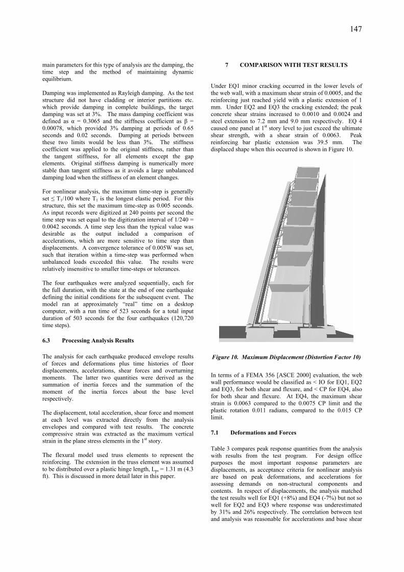
6.1 Model Characteristics The model characteristics were evaluated by extracting periods and mode shapes, by applying a lateral load to define the capacity curve and by applying a lateral displacement to define the wall hysteresis. These steps are intended to verify that model behaviour is as expected. Table 2 lists the first three periods in the direction parallel to the web wall. The fundamental period was 0.56 seconds. The mode shape exhibited a typical cantilever deformation pattern as shown in Figure 7.

Table 2. Periods and Effective Masses

Mode Number

Period (Seconds)

Effective Mass

Cumulative Mass

1 0.557 66.3% 66.3% 5 0.094 17.5% 83.8% 14 0.031 4.7% 88.8%

Figure 7. 1st Mode Shape

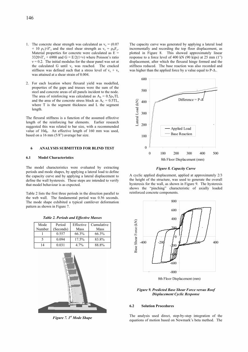
The capacity curve was generated by applying a lateral load incrementally and recording the top floor displacement, as plotted in Figure 8. This showed approximately linear response to a force level of 400 kN (90 kips) at 25 mm (1”) displacement, after which the flexural hinge formed and the stiffness reduced. The base reaction was also recorded and was higher than the applied force by a value equal to P-∆..

0

100

200

300

400

500

600

0 100 200 300 400 5008th Floor Displacement (mm)

Late

ral L

oad

(kN

)

Applied LoadBase Reaction

Difference = P-∆

Figure 8. Capacity Curve

A cyclic applied displacement, applied at approximately 2/3 the height of the structure, was used to generate the overall hysteresis for the wall, as shown in Figure 9. The hysteresis shows the “pinching” characteristic of axially loaded reinforced concrete components.

-800

-600

-400

-200

0

200

400

600

800

-400 -200 0 200 400

8th Floor Displacement (mm)

Bas

e Sh

ear F

orce

(kN

)

Figure 9. Predicted Base Shear Force versus Roof

Displacement Cyclic Response

6.2 Solution Procedures The analysis used direct, step-by-step integration of the equations of motion based on Newmark’s beta method. The

147

main parameters for this type of analysis are the damping, the time step and the method of maintaining dynamic equilibrium. Damping was implemented as Rayleigh damping. As the test structure did not have cladding or interior partitions etc. which provide damping in complete buildings, the target damping was set at 3%. The mass damping coefficient was defined as α = 0.3065 and the stiffness coefficient as β = 0.00078, which provided 3% damping at periods of 0.65 seconds and 0.02 seconds. Damping at periods between these two limits would be less than 3%. The stiffness coefficient was applied to the original stiffness, rather than the tangent stiffness, for all elements except the gap elements. Original stiffness damping is numerically more stable than tangent stiffness as it avoids a large unbalanced damping load when the stiffness of an element changes. For nonlinear analysis, the maximum time-step is generally set ≤ T1/100 where T1 is the longest elastic period. For this structure, this set the maximum time-step as 0.005 seconds. As input records were digitized at 240 points per second the time step was set equal to the digitization interval of 1/240 = 0.0042 seconds. A time step less than the typical value was desirable as the output included a comparison of accelerations, which are more sensitive to time step than displacements. A convergence tolerance of 0.005W was set, such that iteration within a time-step was performed when unbalanced loads exceeded this value. The results were relatively insensitive to smaller time-steps or tolerances. The four earthquakes were analyzed sequentially, each for the full duration, with the state at the end of one earthquake defining the initial conditions for the subsequent event. The model ran at approximately “real” time on a desktop computer, with a run time of 523 seconds for a total input duration of 503 seconds for the four earthquakes (120,720 time steps).

6.3 Processing Analysis Results The analysis for each earthquake produced envelope results of forces and deformations plus time histories of floor displacements, accelerations, shear forces and overturning moments. The latter two quantities were derived as the summation of inertia forces and the summation of the moment of the inertia forces about the base level respectively. The displacement, total acceleration, shear force and moment at each level was extracted directly from the analysis envelopes and compared with test results. The concrete compressive strain was extracted as the maximum vertical strain in the plane stress elements in the 1st story. The flexural model used truss elements to represent the reinforcing. The extension in the truss element was assumed to be distributed over a plastic hinge length, Lp, = 1.31 m (4.3 ft). This is discussed in more detail later in this paper.

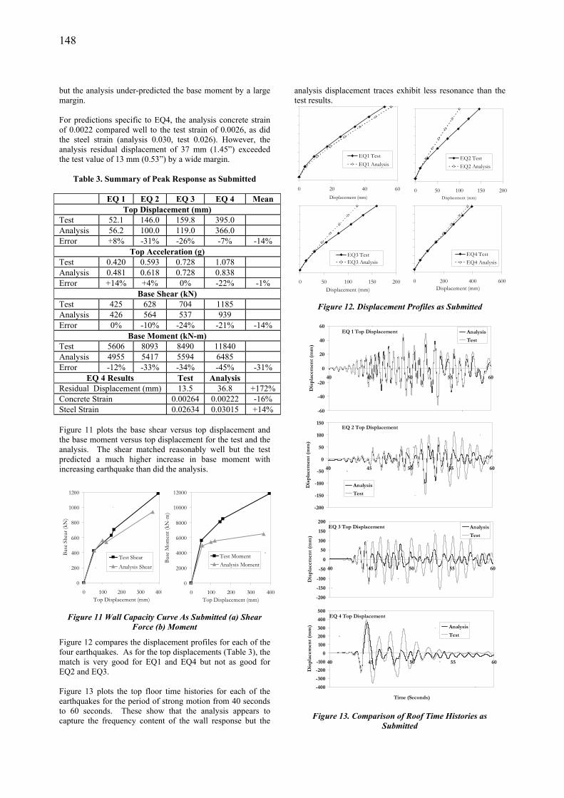
7 COMPARISON WITH TEST RESULTS Under EQ1 minor cracking occurred in the lower levels of the web wall, with a maximum shear strain of 0.0005, and the reinforcing just reached yield with a plastic extension of 1 mm. Under EQ2 and EQ3 the cracking extended; the peak concrete shear strains increased to 0.0010 and 0.0024 and steel extension to 7.2 mm and 9.0 mm respectively. EQ 4 caused one panel at 1st story level to just exceed the ultimate shear strength, with a shear strain of 0.0063. Peak reinforcing bar plastic extension was 39.5 mm. The displaced shape when this occurred is shown in Figure 10.

Figure 10. Maximum Displacement (Distortion Factor 10)

In terms of a FEMA 356 [ASCE 2000] evaluation, the web wall performance would be classified as < IO for EQ1, EQ2 and EQ3, for both shear and flexure, and < CP for EQ4, also for both shear and flexure. At EQ4, the maximum shear strain is 0.0063 compared to the 0.0075 CP limit and the plastic rotation 0.011 radians, compared to the 0.015 CP limit.

7.1 Deformations and Forces Table 3 compares peak response quantities from the analysis with results from the test program. For design office purposes the most important response parameters are displacements, as acceptance criteria for nonlinear analysis are based on peak deformations, and accelerations for assessing demands on non-structural components and contents. In respect of displacements, the analysis matched the test results well for EQ1 (+8%) and EQ4 (-7%) but not so well for EQ2 and EQ3 where response was underestimated by 31% and 26% respectively. The correlation between test and analysis was reasonable for accelerations and base shear

148

but the analysis under-predicted the base moment by a large margin. For predictions specific to EQ4, the analysis concrete strain of 0.0022 compared well to the test strain of 0.0026, as did the steel strain (analysis 0.030, test 0.026). However, the analysis residual displacement of 37 mm (1.45”) exceeded the test value of 13 mm (0.53”) by a wide margin.

Table 3. Summary of Peak Response as Submitted

EQ 1 EQ 2 EQ 3 EQ 4 Mean

Top Displacement (mm) Test 52.1 146.0 159.8 395.0 Analysis 56.2 100.0 119.0 366.0 Error +8% -31% -26% -7% -14%

Top Acceleration (g) Test 0.420 0.593 0.728 1.078 Analysis 0.481 0.618 0.728 0.838 Error +14% +4% 0% -22% -1%

Base Shear (kN) Test 425 628 704 1185 Analysis 426 564 537 939 Error 0% -10% -24% -21% -14%

Base Moment (kN-m) Test 5606 8093 8490 11840 Analysis 4955 5417 5594 6485 Error -12% -33% -34% -45% -31%

EQ 4 Results Test Analysis Residual Displacement (mm) 13.5 36.8 +172% Concrete Strain 0.00264 0.00222 -16% Steel Strain 0.02634 0.03015 +14%

Figure 11 plots the base shear versus top displacement and the base moment versus top displacement for the test and the analysis. The shear matched reasonably well but the test predicted a much higher increase in base moment with increasing earthquake than did the analysis.

0

200

400

600

800

1000

1200

0 100 200 300 400Top Displacement (mm)

Base

She

ar (k

N)

Test Shear

Analysis Shear

0

2000

4000

6000

8000

10000

12000


Base

Mom

ent (

kN-m

)

Test MomentAnalysis Moment

Figure 11 Wall Capacity Curve As Submitted (a) Shear

Force (b) Moment

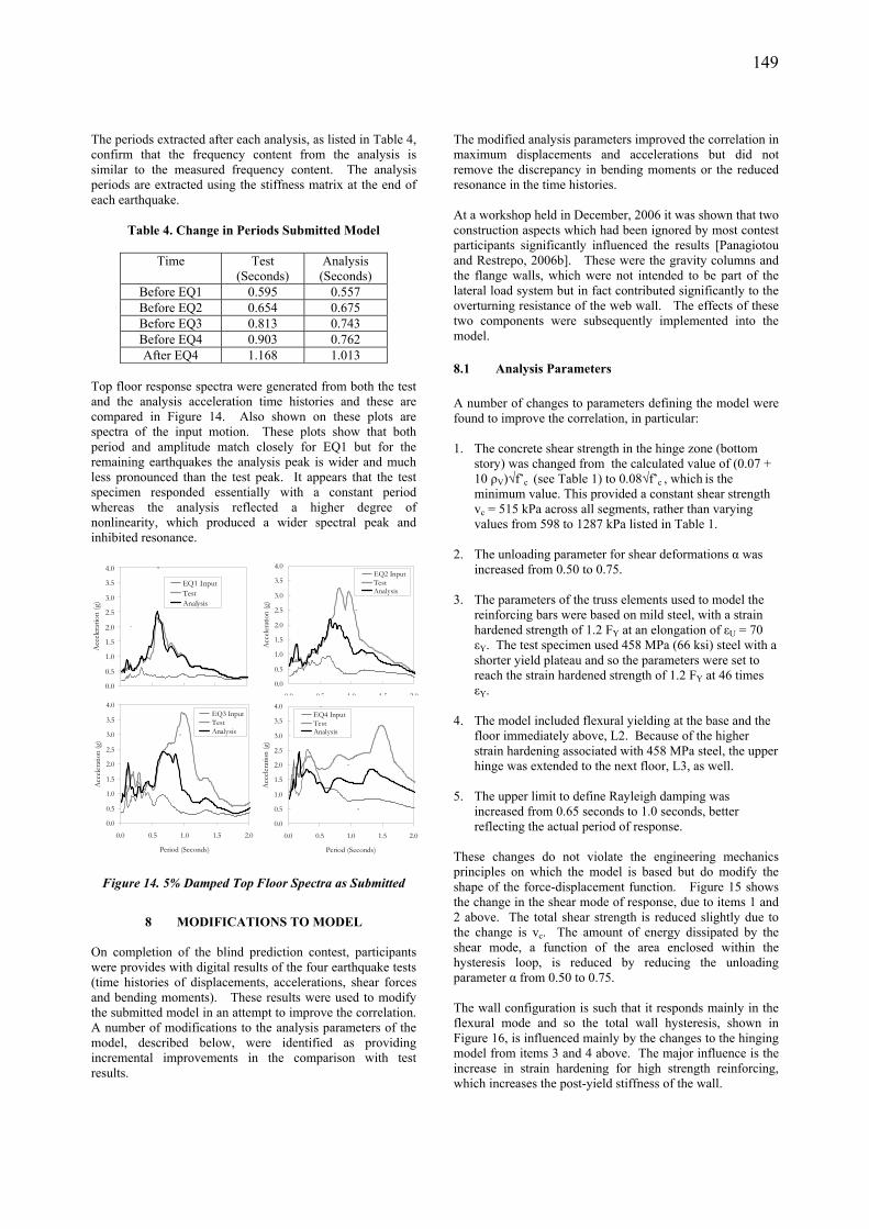
Figure 12 compares the displacement profiles for each of the four earthquakes. As for the top displacements (Table 3), the match is very good for EQ1 and EQ4 but not as good for EQ2 and EQ3. Figure 13 plots the top floor time histories for each of the earthquakes for the period of strong motion from 40 seconds to 60 seconds. These show that the analysis appears to capture the frequency content of the wall response but the

analysis displacement traces exhibit less resonance than the test results.

0 20 40 60Displacement (mm)

EQ1 TestEQ1 Analysis

0 50 100 150 200Displacement (mm)






Figure 12. Displacement Profiles as Submitted

EQ 1 Top Displacement

-60

-40

-20

0

20

40

60

40 45 50 55 60

Dis

pla

cem

ent

(mm

)

Analysis

Test


-200

-150

-100

-50

0

50

100

150

40 45 50 55 60

Dis

pla

cem

ent

(mm

)

Analysis

Test


-200

-150

-100

-50

0

50

100

150

200

40 45 50 55 60

Dis

pla

cem

ent

(mm

)

Analysis

Test


-400

-300

-200

-100

0

100

200

300

400

500

40 45 50 55 60

Time (Seconds)

Dis

pla

cem

ent

(mm

) Analysis

Test

Figure 13. Comparison of Roof Time Histories as

Submitted

149

The periods extracted after each analysis, as listed in Table 4, confirm that the frequency content from the analysis is similar to the measured frequency content. The analysis periods are extracted using the stiffness matrix at the end of each earthquake.

Table 4. Change in Periods Submitted Model

Time Test (Seconds)

Analysis (Seconds)

Before EQ1 0.595 0.557 Before EQ2 0.654 0.675 Before EQ3 0.813 0.743 Before EQ4 0.903 0.762 After EQ4 1.168 1.013

Top floor response spectra were generated from both the test and the analysis acceleration time histories and these are compared in Figure 14. Also shown on these plots are spectra of the input motion. These plots show that both period and amplitude match closely for EQ1 but for the remaining earthquakes the analysis peak is wider and much less pronounced than the test peak. It appears that the test specimen responded essentially with a constant period whereas the analysis reflected a higher degree of nonlinearity, which produced a wider spectral peak and inhibited resonance.

0.0

0.5

1.0

1.5

2.0

2.5

3.0

3.5

4.0

0.0 0.5 1.0 1.5 2.0

Period (Seconds)

Acc

elera

tion

(g)

EQ1 InputTestAnalysis

0.0

0.5

1.0

1.5

2.0

2.5

3.0

3.5

4.0

0.0 0.5 1.0 1.5 2.0

Period (Seconds)

Acc

eler

atio

n (g

)


0.0

0.5

1.0

1.5

2.0

2.5

3.0

3.5

4.0

0.0 0.5 1.0 1.5 2.0

Period (Seconds)

Acc

eler

atio

n (g

)


0.0

0.5

1.0

1.5

2.0

2.5

3.0

3.5

4.0

0.0 0.5 1.0 1.5 2.0

Period (Seconds)

Acc

eler

atio

n (g

)


Figure 14. 5% Damped Top Floor Spectra as Submitted

8 MODIFICATIONS TO MODEL

On completion of the blind prediction contest, participants were provides with digital results of the four earthquake tests (time histories of displacements, accelerations, shear forces and bending moments). These results were used to modify the submitted model in an attempt to improve the correlation. A number of modifications to the analysis parameters of the model, described below, were identified as providing incremental improvements in the comparison with test results.

The modified analysis parameters improved the correlation in maximum displacements and accelerations but did not remove the discrepancy in bending moments or the reduced resonance in the time histories. At a workshop held in December, 2006 it was shown that two construction aspects which had been ignored by most contest participants significantly influenced the results [Panagiotou and Restrepo, 2006b]. These were the gravity columns and the flange walls, which were not intended to be part of the lateral load system but in fact contributed significantly to the overturning resistance of the web wall. The effects of these two components were subsequently implemented into the model.

8.1 Analysis Parameters A number of changes to parameters defining the model were found to improve the correlation, in particular: 1. The concrete shear strength in the hinge zone (bottom

story) was changed from the calculated value of (0.07 + 10 ρV)√f’c (see Table 1) to 0.08√f’c , which is the minimum value. This provided a constant shear strength vc = 515 kPa across all segments, rather than varying values from 598 to 1287 kPa listed in Table 1.

2. The unloading parameter for shear deformations α was

increased from 0.50 to 0.75. 3. The parameters of the truss elements used to model the

reinforcing bars were based on mild steel, with a strain hardened strength of 1.2 FY at an elongation of εU = 70 εY. The test specimen used 458 MPa (66 ksi) steel with a shorter yield plateau and so the parameters were set to reach the strain hardened strength of 1.2 FY at 46 times εY.

4. The model included flexural yielding at the base and the

floor immediately above, L2. Because of the higher strain hardening associated with 458 MPa steel, the upper hinge was extended to the next floor, L3, as well.

5. The upper limit to define Rayleigh damping was

increased from 0.65 seconds to 1.0 seconds, better reflecting the actual period of response.

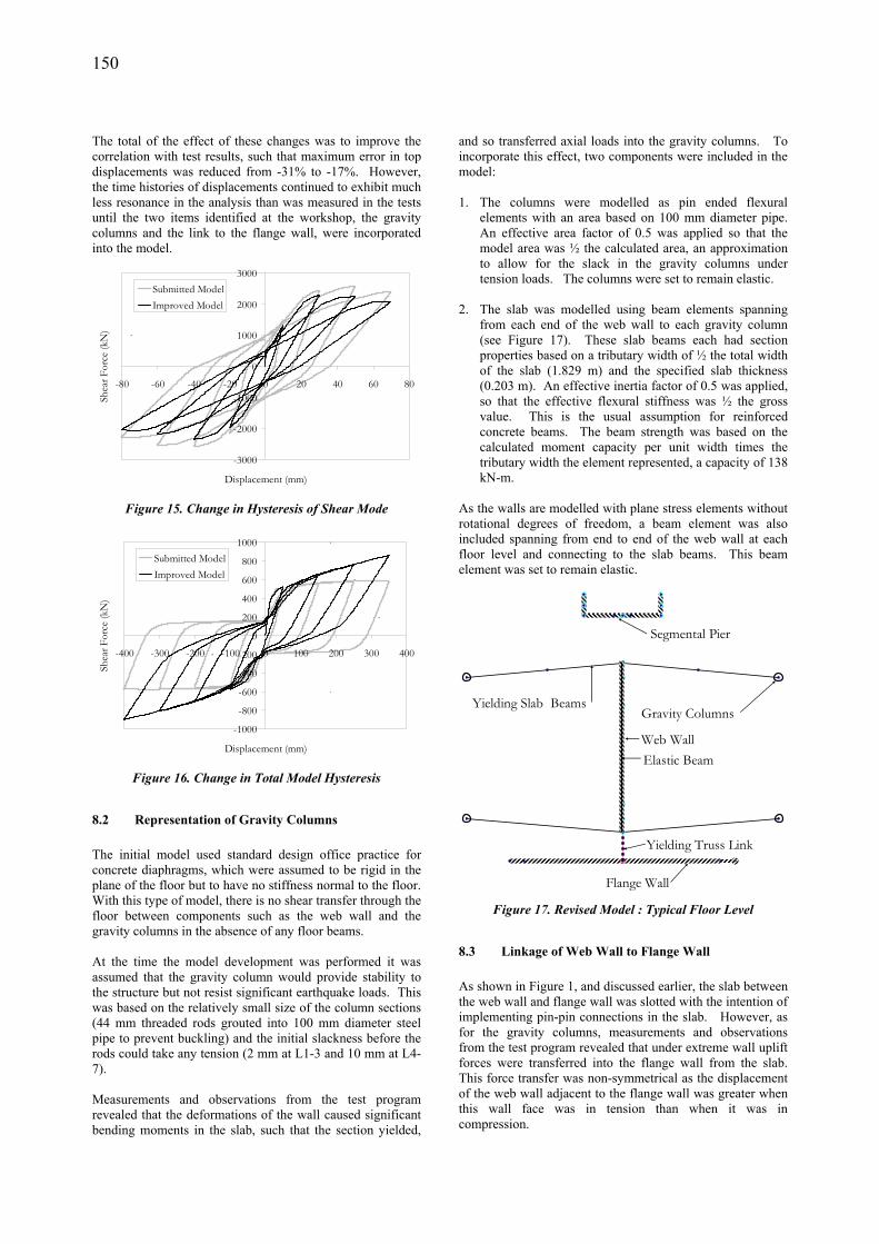
These changes do not violate the engineering mechanics principles on which the model is based but do modify the shape of the force-displacement function. Figure 15 shows the change in the shear mode of response, due to items 1 and 2 above. The total shear strength is reduced slightly due to the change is vc. The amount of energy dissipated by the shear mode, a function of the area enclosed within the hysteresis loop, is reduced by reducing the unloading parameter α from 0.50 to 0.75. The wall configuration is such that it responds mainly in the flexural mode and so the total wall hysteresis, shown in Figure 16, is influenced mainly by the changes to the hinging model from items 3 and 4 above. The major influence is the increase in strain hardening for high strength reinforcing, which increases the post-yield stiffness of the wall.

150

The total of the effect of these changes was to improve the correlation with test results, such that maximum error in top displacements was reduced from -31% to -17%. However, the time histories of displacements continued to exhibit much less resonance in the analysis than was measured in the tests until the two items identified at the workshop, the gravity columns and the link to the flange wall, were incorporated into the model.

-3000

-2000

-1000

0

1000

2000

3000

-80 -60 -40 -20 0 20 40 60 80

Displacement (mm)

Shea

r For

ce (k

N)

Submitted ModelImproved Model

Figure 15. Change in Hysteresis of Shear Mode

-1000

-800

-600

-400

-200

0

200

400

600

800

1000

-400 -300 -200 -100 0 100 200 300 400

Displacement (mm)

Shea

r For

ce (k

N)

Submitted ModelImproved Model

Figure 16. Change in Total Model Hysteresis

8.2 Representation of Gravity Columns The initial model used standard design office practice for concrete diaphragms, which were assumed to be rigid in the plane of the floor but to have no stiffness normal to the floor. With this type of model, there is no shear transfer through the floor between components such as the web wall and the gravity columns in the absence of any floor beams. At the time the model development was performed it was assumed that the gravity column would provide stability to the structure but not resist significant earthquake loads. This was based on the relatively small size of the column sections (44 mm threaded rods grouted into 100 mm diameter steel pipe to prevent buckling) and the initial slackness before the rods could take any tension (2 mm at L1-3 and 10 mm at L4-7). Measurements and observations from the test program revealed that the deformations of the wall caused significant bending moments in the slab, such that the section yielded,

and so transferred axial loads into the gravity columns. To incorporate this effect, two components were included in the model: 1. The columns were modelled as pin ended flexural

elements with an area based on 100 mm diameter pipe. An effective area factor of 0.5 was applied so that the model area was ½ the calculated area, an approximation to allow for the slack in the gravity columns under tension loads. The columns were set to remain elastic.

2. The slab was modelled using beam elements spanning

from each end of the web wall to each gravity column (see Figure 17). These slab beams each had section properties based on a tributary width of ½ the total width of the slab (1.829 m) and the specified slab thickness (0.203 m). An effective inertia factor of 0.5 was applied, so that the effective flexural stiffness was ½ the gross value. This is the usual assumption for reinforced concrete beams. The beam strength was based on the calculated moment capacity per unit width times the tributary width the element represented, a capacity of 138 kN-m.

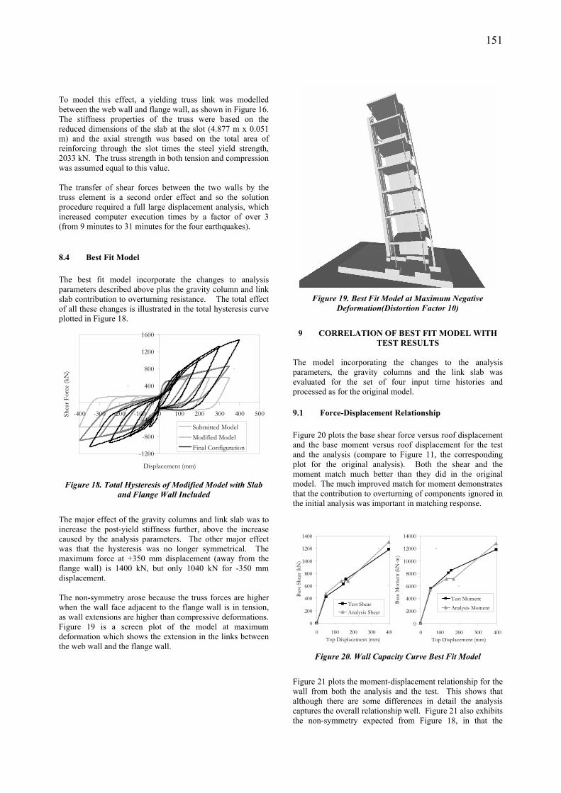
As the walls are modelled with plane stress elements without rotational degrees of freedom, a beam element was also included spanning from end to end of the web wall at each floor level and connecting to the slab beams. This beam element was set to remain elastic.

Web WallElastic Beam

Yielding Slab Beams

Flange Wall

Yielding Truss Link

Gravity Columns

Segmental Pier

Figure 17. Revised Model : Typical Floor Level

8.3 Linkage of Web Wall to Flange Wall As shown in Figure 1, and discussed earlier, the slab between the web wall and flange wall was slotted with the intention of implementing pin-pin connections in the slab. However, as for the gravity columns, measurements and observations from the test program revealed that under extreme wall uplift forces were transferred into the flange wall from the slab. This force transfer was non-symmetrical as the displacement of the web wall adjacent to the flange wall was greater when this wall face was in tension than when it was in compression.

151

To model this effect, a yielding truss link was modelled between the web wall and flange wall, as shown in Figure 16. The stiffness properties of the truss were based on the reduced dimensions of the slab at the slot (4.877 m x 0.051 m) and the axial strength was based on the total area of reinforcing through the slot times the steel yield strength, 2033 kN. The truss strength in both tension and compression was assumed equal to this value. The transfer of shear forces between the two walls by the truss element is a second order effect and so the solution procedure required a full large displacement analysis, which increased computer execution times by a factor of over 3 (from 9 minutes to 31 minutes for the four earthquakes).

8.4 Best Fit Model The best fit model incorporate the changes to analysis parameters described above plus the gravity column and link slab contribution to overturning resistance. The total effect of all these changes is illustrated in the total hysteresis curve plotted in Figure 18.

-1200

-800

-400

0

400

800

1200

1600

-400 -300 -200 -100 0 100 200 300 400 500

Displacement (mm)

Shea

r For

ce (k

N)

Submitted ModelModified ModelFinal Configuration

Figure 18. Total Hysteresis of Modified Model with Slab

and Flange Wall Included

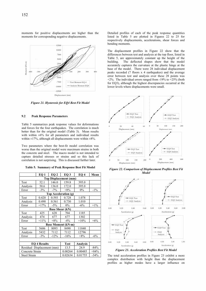
The major effect of the gravity columns and link slab was to increase the post-yield stiffness further, above the increase caused by the analysis parameters. The other major effect was that the hysteresis was no longer symmetrical. The maximum force at +350 mm displacement (away from the flange wall) is 1400 kN, but only 1040 kN for -350 mm displacement. The non-symmetry arose because the truss forces are higher when the wall face adjacent to the flange wall is in tension, as wall extensions are higher than compressive deformations. Figure 19 is a screen plot of the model at maximum deformation which shows the extension in the links between the web wall and the flange wall.

Figure 19. Best Fit Model at Maximum Negative

Deformation(Distortion Factor 10)

9 CORRELATION OF BEST FIT MODEL WITH

TEST RESULTS The model incorporating the changes to the analysis parameters, the gravity columns and the link slab was evaluated for the set of four input time histories and processed as for the original model.

9.1 Force-Displacement Relationship Figure 20 plots the base shear force versus roof displacement and the base moment versus roof displacement for the test and the analysis (compare to Figure 11, the corresponding plot for the original analysis). Both the shear and the moment match much better than they did in the original model. The much improved match for moment demonstrates that the contribution to overturning of components ignored in the initial analysis was important in matching response.

0

200

400

600

800

1000

1200

1400


Base

She

ar (k

N)

Test ShearAnalysis Shear

0

2000

4000

6000

8000

10000

12000

14000


Base

Mom

ent (

kN-m

)

Test Moment

Analysis Moment

Figure 20. Wall Capacity Curve Best Fit Model

Figure 21 plots the moment-displacement relationship for the wall from both the analysis and the test. This shows that although there are some differences in detail the analysis captures the overall relationship well. Figure 21 also exhibits the non-symmetry expected from Figure 18, in that the

152

moments for positive displacements are higher than the moments for corresponding negative displacements.

-12500

-10000

-7500

-5000

-2500

0

2500

5000

7500

10000

12500

-400 -300 -200 -100 0 100 200 300 400

Displacement (mm)

Mom

ent (

kN-m

)

Test Moment-EQ 4Analysis Moment EQ4

Figure 21. Hysteresis for EQ4 Best Fit Model

9.2 Peak Response Parameters Table 5 summarizes peak response values for deformations and forces for the four earthquakes. The correlation is much better than for the original model (Table 3). Mean results with within ±6% for all parameters and individual results within ±17%, although all displacements were within ±8%. Two parameters where the best-fit model correlation was worse than the original model were maximum strains in both the concrete and steel. The macro model is not intended to capture detailed stresses or strains and so this lack of correlation is not surprising. This is discussed further later.

Table 5. Summary of Peak Response Best Fit Model

EQ 1 EQ 2 EQ 3 EQ 4 Mean

Top Displacement (mm) Test 52.1 146.0 159.8 395.0 Analysis 50.6 136.0 172.0 395.0 Error -3% -7% +8% 0% -1%

Top Acceleration (g) Test 0.420 0.593 0.728 1.078 Analysis 0.490 0.561 0.730 1.010 Error +17% -5% 0% -6% +1%

Base Shear (kN) Test 425 628 704 1185 Analysis 474 677 677 1302 Error +11% +8% -4% +10% +6%

Base Moment (kN-m) Test 5606 8093 8490 11840 Analysis 5432 7112 7112 12796 Error -3% -12% -16% +8% -6%

EQ 4 Results Test Analysis

Residual Displacement (mm) 13.5 24.9 -84% Concrete Strain 0.00264 0.00485 +84% Steel Strain 0.02634 0.01755 -34%

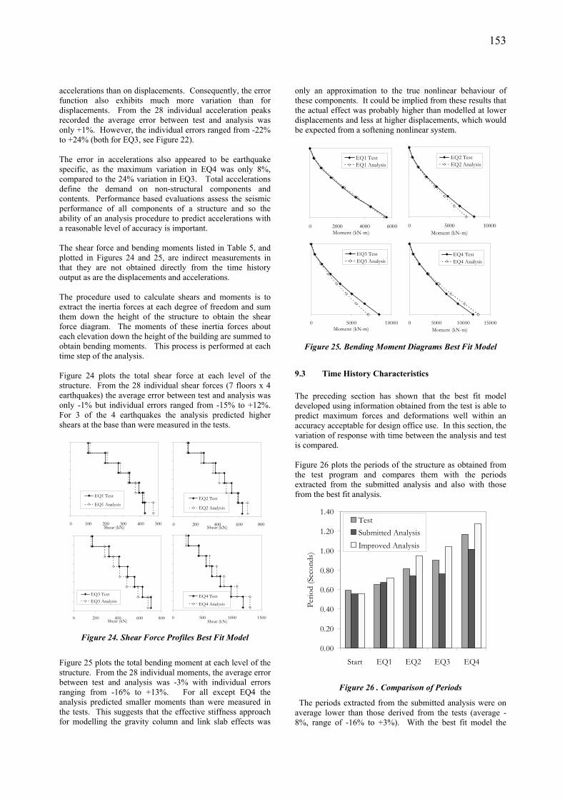
Detailed profiles of each of the peak response quantities listed in Table 5 are plotted in Figures 22 to 25 for respectively displacements, accelerations, shear forces and bending moments. The displacement profiles in Figure 22 show that the differences between test and analysis at the top floor, listed in Table 5, are approximately constant up the height of the building. The deflected shapes show that the model accurately captures the curvature at the plastic hinge at the base of the model. There were 28 individual displacement peaks recorded (7 floors x 4 earthquakes) and the average error between test and analysis over these 28 points was +2%. The individual errors ranged from -19% to +25% (both for EQ3), although the highest discrepancies occurred at the lower levels where displacements were small.




EQ2 Test

EQ2 Analysis


EQ3 Test

EQ3 Analysis



Figure 22. Comparison of Displacement Profiles Best Fit

Model

0.00 0.20 0.40 0.60

Acceleration (g)


0.00 0.20 0.40 0.60 0.80

Acceleration (g)

EQ2 Test

EQ2 Analysis

0.00 0.20 0.40 0.60 0.80

Acceleration (g)

EQ3 Test

EQ3Analysis

0.00 0.50 1.00 1.50

Acceleration (g)

EQ4 Test

EQ4Analysis

Figure 23. Acceleration Profiles Best Fit Model

The total acceleration profiles in Figure 23 exhibit a more complex distribution with height than the displacement profiles as higher modes have a larger influence on

153

accelerations than on displacements. Consequently, the error function also exhibits much more variation than for displacements. From the 28 individual acceleration peaks recorded the average error between test and analysis was only +1%. However, the individual errors ranged from -22% to +24% (both for EQ3, see Figure 22). The error in accelerations also appeared to be earthquake specific, as the maximum variation in EQ4 was only 8%, compared to the 24% variation in EQ3. Total accelerations define the demand on non-structural components and contents. Performance based evaluations assess the seismic performance of all components of a structure and so the ability of an analysis procedure to predict accelerations with a reasonable level of accuracy is important. The shear force and bending moments listed in Table 5, and plotted in Figures 24 and 25, are indirect measurements in that they are not obtained directly from the time history output as are the displacements and accelerations. The procedure used to calculate shears and moments is to extract the inertia forces at each degree of freedom and sum them down the height of the structure to obtain the shear force diagram. The moments of these inertia forces about each elevation down the height of the building are summed to obtain bending moments. This process is performed at each time step of the analysis. Figure 24 plots the total shear force at each level of the structure. From the 28 individual shear forces (7 floors x 4 earthquakes) the average error between test and analysis was only -1% but individual errors ranged from -15% to +12%. For 3 of the 4 earthquakes the analysis predicted higher shears at the base than were measured in the tests.

0 200 400 600 800Shear (kN)


0 100 200 300 400 500Shear (kN)

EQ1 Test

EQ1 Analysis

0 200 400 600 800Shear (kN)

EQ2 Test

EQ2 Analysis

0 500 1000 1500Shear (kN)

EQ4 Test

EQ4 Analysis

Figure 24. Shear Force Profiles Best Fit Model

Figure 25 plots the total bending moment at each level of the structure. From the 28 individual moments, the average error between test and analysis was -3% with individual errors ranging from -16% to +13%. For all except EQ4 the analysis predicted smaller moments than were measured in the tests. This suggests that the effective stiffness approach for modelling the gravity column and link slab effects was

only an approximation to the true nonlinear behaviour of these components. It could be implied from these results that the actual effect was probably higher than modelled at lower displacements and less at higher displacements, which would be expected from a softening nonlinear system.

0 5000 10000Moment (kN-m)


0 5000 10000 15000Moment (kN-m)


0 2000 4000 6000Moment (kN-m)


0 5000 10000Moment (kN-m)


Figure 25. Bending Moment Diagrams Best Fit Model

9.3 Time History Characteristics The preceding section has shown that the best fit model developed using information obtained from the test is able to predict maximum forces and deformations well within an accuracy acceptable for design office use. In this section, the variation of response with time between the analysis and test is compared. Figure 26 plots the periods of the structure as obtained from the test program and compares them with the periods extracted from the submitted analysis and also with those from the best fit analysis.

0.00

0.20

0.40

0.60

0.80

1.00

1.20

1.40

Start EQ1 EQ2 EQ3 EQ4

Perio

d (S

econ

ds)

TestSubmitted AnalysisImproved Analysis

Figure 26 . Comparison of Periods

The periods extracted from the submitted analysis were on average lower than those derived from the tests (average -8%, range of -16% to +3%). With the best fit model the

154

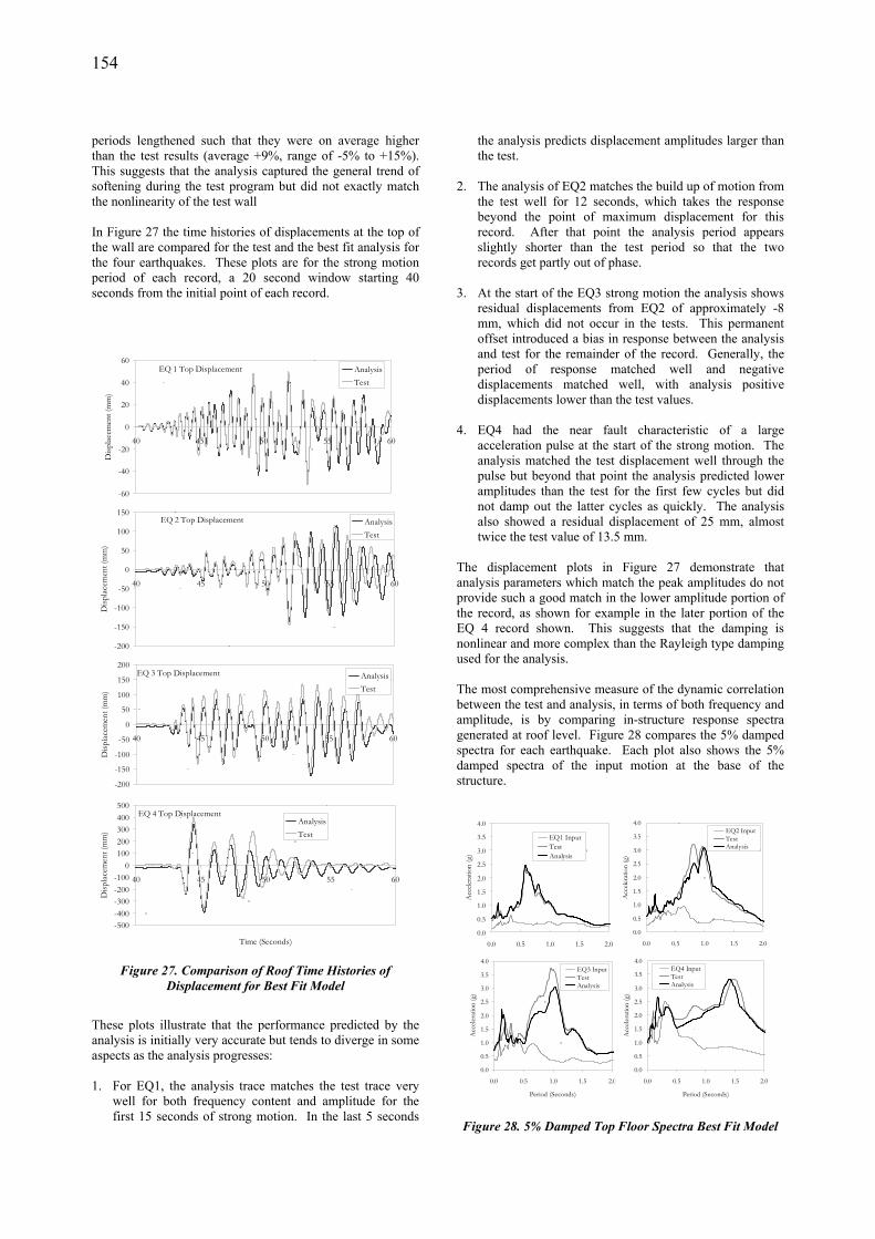
periods lengthened such that they were on average higher than the test results (average +9%, range of -5% to +15%). This suggests that the analysis captured the general trend of softening during the test program but did not exactly match the nonlinearity of the test wall In Figure 27 the time histories of displacements at the top of the wall are compared for the test and the best fit analysis for the four earthquakes. These plots are for the strong motion period of each record, a 20 second window starting 40 seconds from the initial point of each record.


-60

-40

-20

0

20

40

60

40 45 50 55 60

Disp

lace

men

t (m

m)

AnalysisTest


-200

-150

-100

-50

0

50

100

150

40 45 50 55 60

Disp

lace

men

t (m

m)

AnalysisTest


-200

-150

-100

-50

0

50

100

150

200

40 45 50 55 60

Disp

lace

men

t (m

m)

AnalysisTest


-500-400-300-200-100

0100200300400500

40 45 50 55 60

Time (Seconds)

Disp

lace

men

t (m

m)

AnalysisTest

Figure 27. Comparison of Roof Time Histories of

Displacement for Best Fit Model

These plots illustrate that the performance predicted by the analysis is initially very accurate but tends to diverge in some aspects as the analysis progresses: 1. For EQ1, the analysis trace matches the test trace very

well for both frequency content and amplitude for the first 15 seconds of strong motion. In the last 5 seconds

the analysis predicts displacement amplitudes larger than the test.

2. The analysis of EQ2 matches the build up of motion from

the test well for 12 seconds, which takes the response beyond the point of maximum displacement for this record. After that point the analysis period appears slightly shorter than the test period so that the two records get partly out of phase.

3. At the start of the EQ3 strong motion the analysis shows

residual displacements from EQ2 of approximately -8 mm, which did not occur in the tests. This permanent offset introduced a bias in response between the analysis and test for the remainder of the record. Generally, the period of response matched well and negative displacements matched well, with analysis positive displacements lower than the test values.

4. EQ4 had the near fault characteristic of a large

acceleration pulse at the start of the strong motion. The analysis matched the test displacement well through the pulse but beyond that point the analysis predicted lower amplitudes than the test for the first few cycles but did not damp out the latter cycles as quickly. The analysis also showed a residual displacement of 25 mm, almost twice the test value of 13.5 mm.

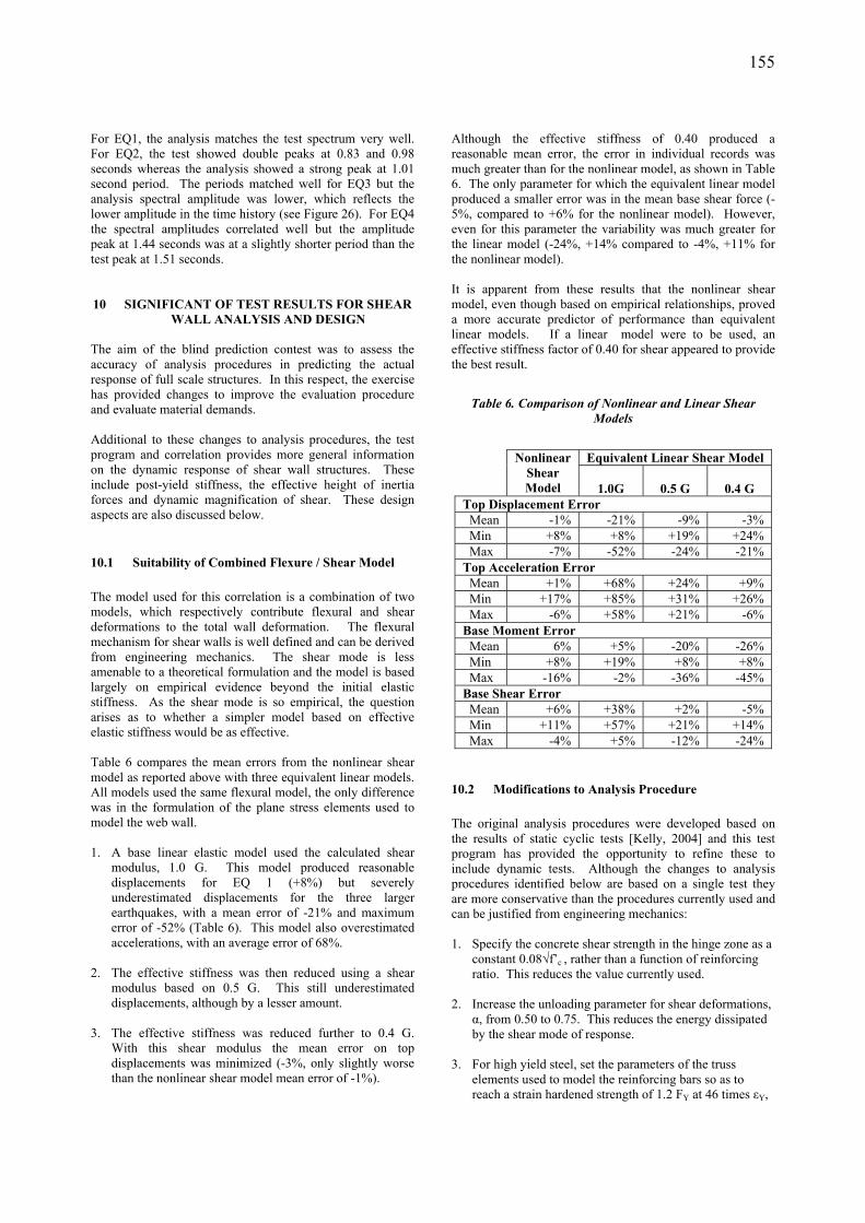
The displacement plots in Figure 27 demonstrate that analysis parameters which match the peak amplitudes do not provide such a good match in the lower amplitude portion of the record, as shown for example in the later portion of the EQ 4 record shown. This suggests that the damping is nonlinear and more complex than the Rayleigh type damping used for the analysis. The most comprehensive measure of the dynamic correlation between the test and analysis, in terms of both frequency and amplitude, is by comparing in-structure response spectra generated at roof level. Figure 28 compares the 5% damped spectra for each earthquake. Each plot also shows the 5% damped spectra of the input motion at the base of the structure.

0.0

0.5

1.0

1.5

2.0

2.5

3.0

3.5

4.0

0.0 0.5 1.0 1.5 2.0

Period (Seconds)

Acc

elera

tion

(g)


0.0

0.5

1.0

1.5

2.0

2.5

3.0

3.5

4.0

0.0 0.5 1.0 1.5 2.0

Period (Seconds)

Acc

eler

atio

n (g

)


0.0

0.5

1.0

1.5

2.0

2.5

3.0

3.5

4.0

0.0 0.5 1.0 1.5 2.0

Period (Seconds)

Acc

eler

atio

n (g

)


0.0

0.5

1.0

1.5

2.0

2.5

3.0

3.5

4.0

0.0 0.5 1.0 1.5 2.0

Period (Seconds)

Acc

eler

atio

n (g

)


Figure 28. 5% Damped Top Floor Spectra Best Fit Model

155

For EQ1, the analysis matches the test spectrum very well. For EQ2, the test showed double peaks at 0.83 and 0.98 seconds whereas the analysis showed a strong peak at 1.01 second period. The periods matched well for EQ3 but the analysis spectral amplitude was lower, which reflects the lower amplitude in the time history (see Figure 26). For EQ4 the spectral amplitudes correlated well but the amplitude peak at 1.44 seconds was at a slightly shorter period than the test peak at 1.51 seconds. 10 SIGNIFICANT OF TEST RESULTS FOR SHEAR

WALL ANALYSIS AND DESIGN The aim of the blind prediction contest was to assess the accuracy of analysis procedures in predicting the actual response of full scale structures. In this respect, the exercise has provided changes to improve the evaluation procedure and evaluate material demands. Additional to these changes to analysis procedures, the test program and correlation provides more general information on the dynamic response of shear wall structures. These include post-yield stiffness, the effective height of inertia forces and dynamic magnification of shear. These design aspects are also discussed below.

10.1 Suitability of Combined Flexure / Shear Model The model used for this correlation is a combination of two models, which respectively contribute flexural and shear deformations to the total wall deformation. The flexural mechanism for shear walls is well defined and can be derived from engineering mechanics. The shear mode is less amenable to a theoretical formulation and the model is based largely on empirical evidence beyond the initial elastic stiffness. As the shear mode is so empirical, the question arises as to whether a simpler model based on effective elastic stiffness would be as effective. Table 6 compares the mean errors from the nonlinear shear model as reported above with three equivalent linear models. All models used the same flexural model, the only difference was in the formulation of the plane stress elements used to model the web wall. 1. A base linear elastic model used the calculated shear

modulus, 1.0 G. This model produced reasonable displacements for EQ 1 (+8%) but severely underestimated displacements for the three larger earthquakes, with a mean error of -21% and maximum error of -52% (Table 6). This model also overestimated accelerations, with an average error of 68%.

2. The effective stiffness was then reduced using a shear

modulus based on 0.5 G. This still underestimated displacements, although by a lesser amount.

3. The effective stiffness was reduced further to 0.4 G.

With this shear modulus the mean error on top displacements was minimized (-3%, only slightly worse than the nonlinear shear model mean error of -1%).

Although the effective stiffness of 0.40 produced a reasonable mean error, the error in individual records was much greater than for the nonlinear model, as shown in Table 6. The only parameter for which the equivalent linear model produced a smaller error was in the mean base shear force (-5%, compared to +6% for the nonlinear model). However, even for this parameter the variability was much greater for the linear model (-24%, +14% compared to -4%, +11% for the nonlinear model). It is apparent from these results that the nonlinear shear model, even though based on empirical relationships, proved a more accurate predictor of performance than equivalent linear models. If a linear model were to be used, an effective stiffness factor of 0.40 for shear appeared to provide the best result.

Table 6. Comparison of Nonlinear and Linear Shear Models

Equivalent Linear Shear Model

Nonlinear Shear Model

1.0G

0.5 G

0.4 G

Top Displacement Error Mean -1% -21% -9% -3% Min +8% +8% +19% +24% Max -7% -52% -24% -21% Top Acceleration Error Mean +1% +68% +24% +9% Min +17% +85% +31% +26% Max -6% +58% +21% -6% Base Moment Error Mean 6% +5% -20% -26% Min +8% +19% +8% +8% Max -16% -2% -36% -45% Base Shear Error Mean +6% +38% +2% -5% Min +11% +57% +21% +14% Max -4% +5% -12% -24%

10.2 Modifications to Analysis Procedure The original analysis procedures were developed based on the results of static cyclic tests [Kelly, 2004] and this test program has provided the opportunity to refine these to include dynamic tests. Although the changes to analysis procedures identified below are based on a single test they are more conservative than the procedures currently used and can be justified from engineering mechanics: 1. Specify the concrete shear strength in the hinge zone as a

constant 0.08√f’c , rather than a function of reinforcing ratio. This reduces the value currently used.

2. Increase the unloading parameter for shear deformations,

α, from 0.50 to 0.75. This reduces the energy dissipated by the shear mode of response.

3. For high yield steel, set the parameters of the truss

elements used to model the reinforcing bars so as to reach a strain hardened strength of 1.2 FY at 46 times εY,

156

compared to the default value of 1.2 FY at an elongation of 70 εY for mild steel.

4. For high strength steel, because of the higher strain

hardening than mild steel, it will sometimes be advisable to model hinging at upper levels to allow for hinge spreading.

5. It may be advisable to increase the upper period limit

used to define Rayleigh damping to reflect the actual period of response. In this case, a period of 1.5 times the elastic period provided a better representation of actual damping.

For this evaluation Rayleigh damping using coefficients on the mass matrix and original stiffness matrix so as to provide 3% of critical damping provided the best correlation with test results. As the model did not include components such as cladding or non-structural components, there is no evidence to suggest changing the design office practice of specifying 5% Rayleigh damping for complete buildings.

10.3 Evaluating Material Performance The analysis procedure provides the maximum extension in the truss elements representing the reinforcing bars. To convert this to steel strain, as provided from test results, the extension is divided by a plastic hinge length. A formula for the plastic hinge length, Lp, [Priestley, 2000] is the greater of:

nwp hLL 03.02.0 += (1a)

bynp dfhL 022.0054.0 += (1b) where Lw = length of wall, hn = wall height and db and fy are the diameter and yield stress of the vertical reinforcing. For this wall, equation (1a) governs and provides a plastic hinge length of 1.31m. The test steel strains measured in the test [Panagiotou et al 2006a] under EQ 4 reached the maximum of approximately 0.025 at strain gauges at elevations 0.254m, 0.762 m and 1.27 m (10”, 30” and 50”) and reduced to 0.005 at 1.524 m (60”). This implies a plastic hinge length of approximately 1.27m, which corresponds well to the Priestley value of 1.31m. The maximum truss extension from each analysis was divided by this value to obtain strains. The maximum concrete strain was assumed to be the vertical strain in the plane stress elements representing the web wall in the lowest story. Table 7 lists the test strains and the maximum strains from the submitted model, the model with modified parameters but no gravity column or link and the final best fit model which included gravity column and the links. The submitted analysis values were reasonable close to the test value, with both steel strain and concrete strain within 15%. However, the best fit match was not as good, with steel strains 35% less than the test results and concrete strains 85% higher. In terms of steel strain, the modified analysis in which the analysis parameters were varied but the gravity columns and links ignored provided a steel strain within 4% of the test value. It appears that the approximate representation of the

gravity columns and links improved the overall correlation but resulted in less accuracy in the reinforcing bar response.

Table 7. Material Strains

Steel

Strain (mm/mm)

Concrete Strain

(mm/mm) Test 0.026 0.0026 Submitted Analysis 0.030

+14% 0.0022 -15%

Modified Analysis (No gravity column / flange wall)

0.027 +4%

0.0047 +81%

Best Fit Analysis 0.017 -35%

0.0048 +85%

The use of equations (1a and 1b) is only an approximation for this application and this may explain the discrepancy. These equations were developed for cases where plasticity can spread freely, such as bridge columns. In buildings the spread of plasticity may be constrained by the reinforcement detailing and construction staging and this was the case in the tested building tested. Therefore, although there appears to be a good agreement between these equations and the measured spread, this may be more apparent than real as the equations are for the equivalent plastic hinge length and the measured strains are for the actual spread. In some cases, such as for longer walls, there may be substantial differences. For concrete strains, the type of macro model used here would not be expected to predict maximum values and the relatively close match in the submitted analysis was most likely coincidental. The strains listed in the evaluation are taken from the coarse modelling, where a single panel represents a full story height and this resolution could not be expected to provide an accurate strain distribution. The evaluation procedures do not rely on concrete strains and so this restriction does not inhibit use of the procedures.

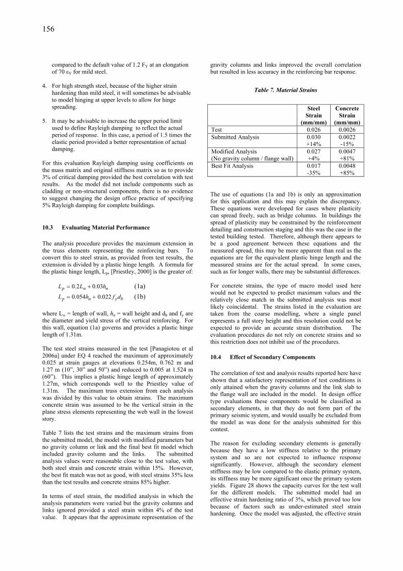
10.4 Effect of Secondary Components The correlation of test and analysis results reported here have shown that a satisfactory representation of test conditions is only attained when the gravity columns and the link slab to the flange wall are included in the model. In design office type evaluations these components would be classified as secondary elements, in that they do not form part of the primary seismic system, and would usually be excluded from the model as was done for the analysis submitted for this contest. The reason for excluding secondary elements is generally because they have a low stiffness relative to the primary system and so are not expected to influence response significantly. However, although the secondary element stiffness may be low compared to the elastic primary system, its stiffness may be more significant once the primary system yields. Figure 28 shows the capacity curves for the test wall for the different models. The submitted model had an effective strain hardening ratio of 3%, which proved too low because of factors such as under-estimated steel strain hardening. Once the model was adjusted, the effective strain

157

hardening increased to 8%. When the gravity columns and the link to the flange wall were included in the model the strain hardening increased further to 15%.

0

100

200

300

400

500

600

700

800

0 100 200 300 400Roof Displacement (mm)

Late

ral L

oad

(kN

)

As Submitted 3% S.H.R.Adjusted Model 8% S.H.R.Final Model 15% S.H.R.

Figure 29. Effective Strain Hardening Ratio (S.H.R)

It can be implied from the capacity curves that the average stiffness of the “secondary” components in the final model is the difference in yielded stiffness, which is 15% - 8% = 7% of the primary system stiffness. However, the effect on the maximum wall moment was much more than this. The average error (analysis moment to test moment) for the four earthquakes was -19%, which improved to -6% when the secondary components were included.

10.5 Dynamic Magnification of Shear Under the capacity design principles used in New Zealand the shear force in a cantilever wall is limited to the shear at the time the maximum base moment, including all sources of overstrength, occurs. However, a number of studies have shown that under dynamic loads the shear force may increase beyond this overstrength shear [Blakeley et al 1975]. To account for this, the shear force is factored by a dynamic magnification factor, ωv, to develop upper bound shear forces [Standards New Zealand, 1995]. The dynamic magnification factor is a function of the number of storeys, N, calculated as follows:

10/9.0 Nv +=ω for buildings up to 6 storeys, and

8.130/3.1 ≤+= Nvω for buildings over 6 storeys. For a cantilever the shear force is calculated from the base moment M as V = M/hEFF, where hEFF is the effective height of application of the force. As M is limited to the overstrength moment capacity of the wall, it is apparent that

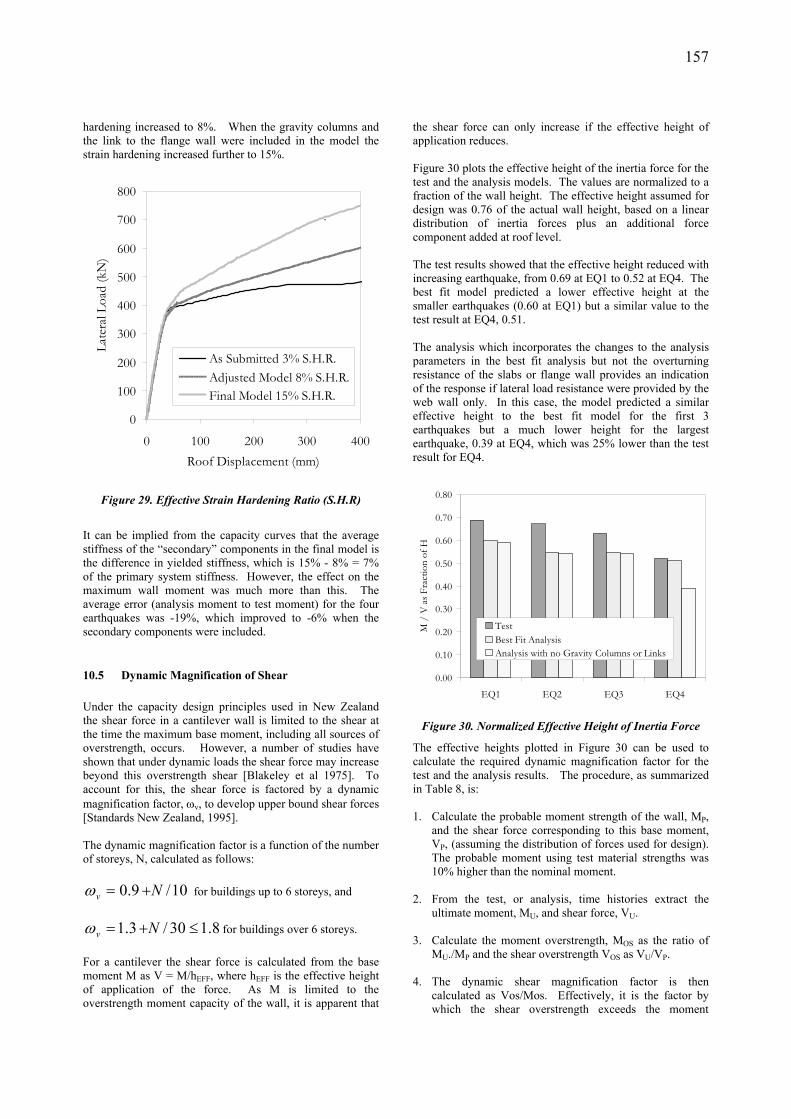
the shear force can only increase if the effective height of application reduces. Figure 30 plots the effective height of the inertia force for the test and the analysis models. The values are normalized to a fraction of the wall height. The effective height assumed for design was 0.76 of the actual wall height, based on a linear distribution of inertia forces plus an additional force component added at roof level. The test results showed that the effective height reduced with increasing earthquake, from 0.69 at EQ1 to 0.52 at EQ4. The best fit model predicted a lower effective height at the smaller earthquakes (0.60 at EQ1) but a similar value to the test result at EQ4, 0.51. The analysis which incorporates the changes to the analysis parameters in the best fit analysis but not the overturning resistance of the slabs or flange wall provides an indication of the response if lateral load resistance were provided by the web wall only. In this case, the model predicted a similar effective height to the best fit model for the first 3 earthquakes but a much lower height for the largest earthquake, 0.39 at EQ4, which was 25% lower than the test result for EQ4.

0.00

0.10

0.20

0.30

0.40

0.50

0.60

0.70

0.80

EQ1 EQ2 EQ3 EQ4

M /

V a

s Fra

ctio

n of

H

TestBest Fit AnalysisAnalysis with no Gravity Columns or Links

Figure 30. Normalized Effective Height of Inertia Force

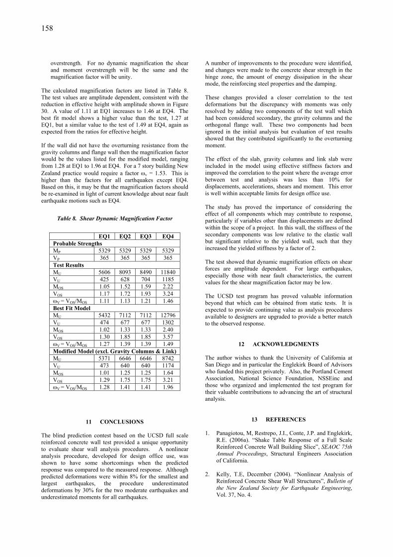
The effective heights plotted in Figure 30 can be used to calculate the required dynamic magnification factor for the test and the analysis results. The procedure, as summarized in Table 8, is: 1. Calculate the probable moment strength of the wall, MP,

and the shear force corresponding to this base moment, VP, (assuming the distribution of forces used for design). The probable moment using test material strengths was 10% higher than the nominal moment.

2. From the test, or analysis, time histories extract the

ultimate moment, MU, and shear force, VU. 3. Calculate the moment overstrength, MOS as the ratio of

MU./MP and the shear overstrength VOS as VU/VP. 4. The dynamic shear magnification factor is then

calculated as Vos/Mos. Effectively, it is the factor by which the shear overstrength exceeds the moment

158

overstrength. For no dynamic magnification the shear and moment overstrength will be the same and the magnification factor will be unity.

The calculated magnification factors are listed in Table 8. The test values are amplitude dependent, consistent with the reduction in effective height with amplitude shown in Figure 30. A value of 1.11 at EQ1 increases to 1.46 at EQ4. The best fit model shows a higher value than the test, 1.27 at EQ1, but a similar value to the test of 1.49 at EQ4, again as expected from the ratios for effective height. If the wall did not have the overturning resistance from the gravity columns and flange wall then the magnification factor would be the values listed for the modified model, ranging from 1.28 at EQ1 to 1.96 at EQ4. For a 7 story building New Zealand practice would require a factor ωv = 1.53. This is higher than the factors for all earthquakes except EQ4. Based on this, it may be that the magnification factors should be re-examined in light of current knowledge about near fault earthquake motions such as EQ4.

Table 8. Shear Dynamic Magnification Factor

EQ1 EQ2 EQ3 EQ4 Probable Strengths MP 5329 5329 5329 5329 VP 365 365 365 365 Test Results MU 5606 8093 8490 11840 VU 425 628 704 1185 MOS 1.05 1.52 1.59 2.22 VOS 1.17 1.72 1.93 3.24 ωV = VOS/MOS 1.11 1.13 1.21 1.46 Best Fit Model MU 5432 7112 7112 12796 VU 474 677 677 1302 MOS 1.02 1.33 1.33 2.40 VOS 1.30 1.85 1.85 3.57 ωV = VOS/MOS 1.27 1.39 1.39 1.49 Modified Model (excl. Gravity Columns & Link) MU 5371 6646 6646 8742 VU 473 640 640 1174 MOS 1.01 1.25 1.25 1.64 VOS 1.29 1.75 1.75 3.21 ωV = VOS/MOS 1.28 1.41 1.41 1.96

11 CONCLUSIONS The blind prediction contest based on the UCSD full scale reinforced concrete wall test provided a unique opportunity to evaluate shear wall analysis procedures. A nonlinear analysis procedure, developed for design office use, was shown to have some shortcomings when the predicted response was compared to the measured response. Although predicted deformations were within 8% for the smallest and largest earthquakes, the procedure underestimated deformations by 30% for the two moderate earthquakes and underestimated moments for all earthquakes.

A number of improvements to the procedure were identified, and changes were made to the concrete shear strength in the hinge zone, the amount of energy dissipation in the shear mode, the reinforcing steel properties and the damping. These changes provided a closer correlation to the test deformations but the discrepancy with moments was only resolved by adding two components of the test wall which had been considered secondary, the gravity columns and the orthogonal flange wall. These two components had been ignored in the initial analysis but evaluation of test results showed that they contributed significantly to the overturning moment. The effect of the slab, gravity columns and link slab were included in the model using effective stiffness factors and improved the correlation to the point where the average error between test and analysis was less than 10% for displacements, accelerations, shears and moment. This error is well within acceptable limits for design office use. The study has proved the importance of considering the effect of all components which may contribute to response, particularly if variables other than displacements are defined within the scope of a project. In this wall, the stiffness of the secondary components was low relative to the elastic wall but significant relative to the yielded wall, such that they increased the yielded stiffness by a factor of 2. The test showed that dynamic magnification effects on shear forces are amplitude dependent. For large earthquakes, especially those with near fault characteristics, the current values for the shear magnification factor may be low. The UCSD test program has proved valuable information beyond that which can be obtained from static tests. It is expected to provide continuing value as analysis procedures available to designers are upgraded to provide a better match to the observed response.

12 ACKNOWLEDGMENTS The author wishes to thank the University of California at San Diego and in particular the Englekirk Board of Advisors who funded this project privately. Also, the Portland Cement Association, National Science Foundation, NSSEinc and those who organized and implemented the test program for their valuable contributions to advancing the art of structural analysis.

13 REFERENCES 1. Panagiotou, M, Restrepo, J.I., Conte, J.P. and Englekirk,

R.E. (2006a). “Shake Table Response of a Full Scale Reinforced Concrete Wall Building Slice”, SEAOC 75th Annual Proceedings, Structural Engineers Association of California.

2. Kelly, T.E, December (2004). “Nonlinear Analysis of

Reinforced Concrete Shear Wall Structures”, Bulletin of the New Zealand Society for Earthquake Engineering, Vol. 37, No. 4.

159

3. Kelly, T. E., (2006). “NCEES Blind Prediction Test: Practitioner Entry from Holmes Consulting Group”, NEES/UCSD Workshop on Analytical Modeling of Reinforced Masonry Walls, San Diego, CA. December.

4. Panagiotou, M., and Restrepo, J.I., (2006b). “Model

Calibration for the UCSD 7-Story Building Slice”, NEES/UCSD Workshop on Analytical Modeling of Reinforced Masonry Walls, San Diego, CA., December.

5. ASCE, American Society of Civil Engineers, (2000).

“Prestandard and Commentary for the Seismic Rehabilitation of Buildings”, prepared for the SAC Joint Venture, published by the Federal Emergency Management Agency FEMA-356, Washington, D.C.

6. Mondkar, D.P. and Powell, G.H., (1979). “ANSR II

Analysis of Non-linear Structural Resonse User's Manual”, Earthquake Engrg. Research Center EERC 79/17, University of California, Berkeley, July.

7. Priestley, M. J. N., (2000). Performance Based Seismic

Design, 12th World Conference on Earthquake Engineering, Auckland, New Zealand.

8. Blakeley, R.W.G, Cooney, R.C and Megget, L.M.

(1975). “Seismic Shear Loading at Flexural Capacity in Cantilever Wall Structures”, Bulletin of the New Zealand National Society for Earthquake Engineering, Vol. 8 No. 4.

9. Standards New Zealand, (1995). Concrete Structures

Standard : Part 1 - The Design of Concrete Structures, NZS 3101:Part 1:1995.

Documents

A BLIND PREDICTION TEST OF NONLINEAR ANALYSIS …3)0142.pdf · 142 A BLIND PREDICTION TEST OF NONLINEAR ANALYSIS PROCEDURES FOR REINFORCED CONCRETE SHEAR WALLS Trevor Kelly1 ABSTRACT