i i §J ^W? If . ifw Q.t& 'hr^fJt-

ft

W t upafrn

lit J ~* "*

* *

s

£

ORNL-4S75, Volu*r* 1 UC-25 - Me att, Cematcs, and Matariab

CORROSION IN POLYTHERMAL LOOP SYSTEMS.

!. MASS t.lANSFER LlMiTED BY SURFACE AND

INTERFACE RESISTANCES AS COMPARED

WITH SODIUM-INCQNEL BEHAVIOR

3 . ft. Eur ; HI Paul Nelson, Jr.

OAK RIDGE NATIONAL LABORATORY operated by

U N I O N CARBIDE CORPORATION lor the

U.S. ATOMIC ENERGY C O M M I S S I O N

:••': ;r '/;:;:-• '•;*->€'-VTN7 (S iJMUWTTf:*

Dl * I I I / nJH B" BLHNK PAGE

-&< ^%3l8fe.. »_

rr-*^w-

BSE ~s"S7 '""•s.'i? v»-.l " S ^ ^ < I M >

-**!" Printed to the UnHtJSum «f Amgrict M t i i * *ron *•****« Te&fetf «cfom*r snfttvic*

SSfrfottfto? j | ffc»^Seri**fi**d, Vegifel* 2 2 W

« ^ <

n i i i i <i I "'liiti ii««

1 P

»- *'n> ' * M I « ^ I

m m wxount <# mot*: «pan»rn»t ^ ^ T *» VHtmt $tmm saar" «w Uftiutf

i-w of 'flitii- WTMilcrwL ncf MT» a£

1 Uu*d J Atomic I

& ? # ; 3 ^ * ^ | f t l * * M «i * P JBHwwar i m ^ pro** or ll##^^*fT^W^j 1fcP*

or

»Bfy^ht j.? s»-; ,-r; flQjRTE,

*^Ki^H9M^W''*r«l J J '

.1 ii

3

%*>

•

BLANK PAGE

ORNL^4575

Contract No. W-7405-eng-26

METALS AND CERAMICS DIVISION

CORROSION IN POLYTHERMAL LOOP SYSTEMS.

I. MASS TRANSFER LIMITED BY SURFACE AND INTERFACE RESISTANCES AS COMPARED

WITH SODIUM-INCONEL BEHAVIOR

R. B. Evans III Pau' Nelson, Jr.

I S « 5 A I N O T I C E prepared as an acco^s: cf work This report

sponsored by the* United stares '~M»*>^ •«•«££. N-siU—; the United SUtes nor the United States Atomic Energy Commission, nor any of their employees, nor any of their contractors, subcontractors, or their employees, tnakes any warranty, express or implied, or assumes any legal ttabnr'.y or responsibility for the accuracy, com. pteteness <*r usefulness of any information, apparatus, product or process drsdoaed, or represents that its use would not infringe prhratety owned rights.

MARCH 1971

OAK RIOGE NATIONAL LABORATORY Oak RMfJ, Tiriiianjni

QOQfmBB oy UNION CARBIDE CORPORATION

for«M U. S. ATOMIC ENERGY COMMISSION

' « <'}r<-

I l l

CONTENTS

Abstract 1

lntroduct:on I

Nomenclature . . . . 4

Temperature Profiles and Loop Configurations 6 Reference and Prototype Loops 6

The Reference Loop 6 Prototype L.x>ps 7

Considerations Concerning the Temperature Variation of the Solubility Reaction 9

Mass-Transfer Equations 10 The General Equation 10

The Differential Equation 10 Integration Procedures 12

Transient Behavior !5

Steady-State Solutions 16 The "Tent-Shaped" Y{z) Function 16

The Combined Form 16 Related Temperature Functions 18 Periodicity and Symmetry 18 Computation of Mass Transfer 20

The Exact Solution 20 Approximate Form for Low 0 22

The "Saw-Tooth" Y{z) Function 24 More About the Approach to Steady State 26 Steady-State Solution for Various 0 Values 26 Computation of Mass Transfer 28

Discussion 30 Concerning the General Solution 30 Application to Corrosion in Sodium-Inconel Systems 31

Closure 35

Appendix A. Computation of the Constant 0 for Mass Transfer 36

Appendix B. Computation of the Constant 0' for Heat Transfer 36

Appendix C. Temperature Profile Equations for the Prototype Loop 37

Appendix D. Combined Solution-Rate and Film Coefficient 39

CORROSION IN POLYTHERMAL LOOP SYSTEMS.

I. MASS TRANSFER LIMITED BY SURFACE AND INTERFACE RESISTANCES AS COMPARED WITH SODIUM-INCONEL BEHAVIOR

R. B- Evans III» Paul Nelson, Jr. 2

ABSTRACT

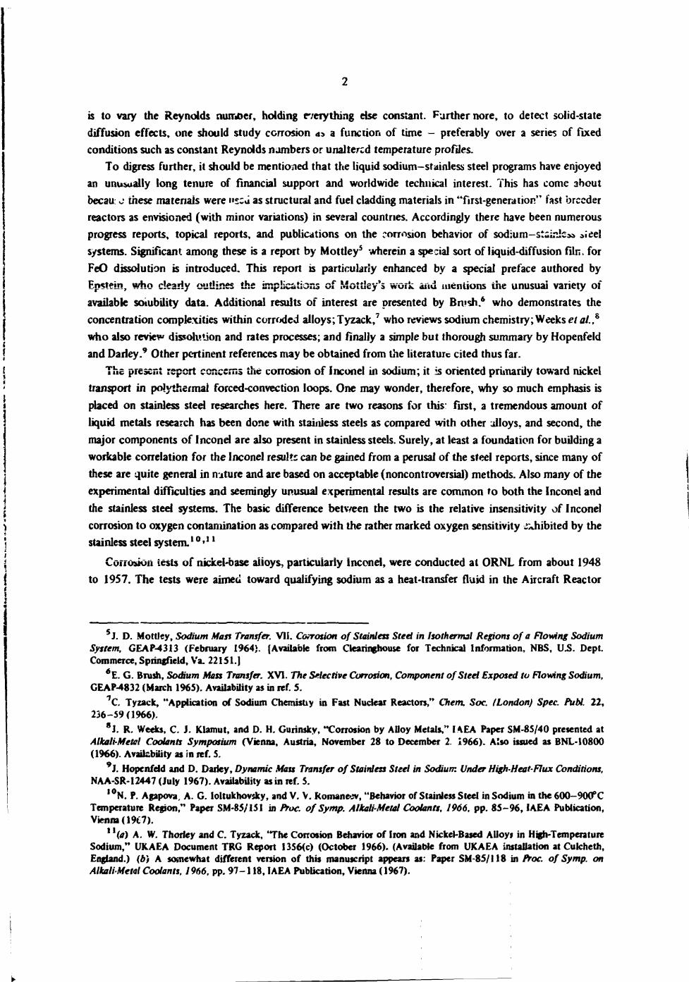
Ccrxosion studies of Inconel v.d similar nickd-base alloys in flowing sodium have shown that considerable quantities of nickel are removed from regjors hotter than l?(Xf F and deposited in cooler regions. We have compared the observed w « A * y « l M A W l i ^ M f ' M • - ^ • • ^ *a»*+l» WWkrfl*^»t«./V«** t * n » A s 4 *« * * + % » A ^ ^ * * * M W M * « * « • * * V « J » + - 4 « # V * B * * * « « * s>f «%*s*lr4*1 ^ * * « * * * # * + l « A f*««>ra*9 lw/%**»«J^*Wr « f » ^ % « H l i t i H i l l " * * " * « H ^ d * * • » « • f * * M J b U V S M W O J » M V U U I V M J i H I I I W U V H U14KI V * X « t * * 9 * V l * V « l i r r " ->« *n*a«S.»> * * « * • f ^ f i»«W W W 1 " « « ( J

layer at the alloy surface controls the process. For pumped loops operating in ihe turbulent flow regime, it was demonstrated analytically that the time transient

required to achieve steady-state mass-transfer conditions is relatively short compared with normal loop operating times. Based on a cakulated fibn coefficient, the predicted transport of nickel from the hot zone was five times greater than that obtained from measurements of crystal deposits in cold zones. This and other considerations suggest that contributions of film resistances are only partially responsible for corrciioa in poly thermal loops containing liquid metals. In other words, a complete description of the corrosion proces will require considerable modification of the mechanism discussed here.

AM results were derived from a simple partial differential equation which is first order with respect to time and position. The solution of the differential equation is found in closed form; accordingly, it can be readily manipulated to exhibit the tnmsent and steady-state parts. The solution will accommodate a wide variety of assumed experimental conditions. It holds Tor heat- at well as mass-transfer problems.

INTRODUCTION

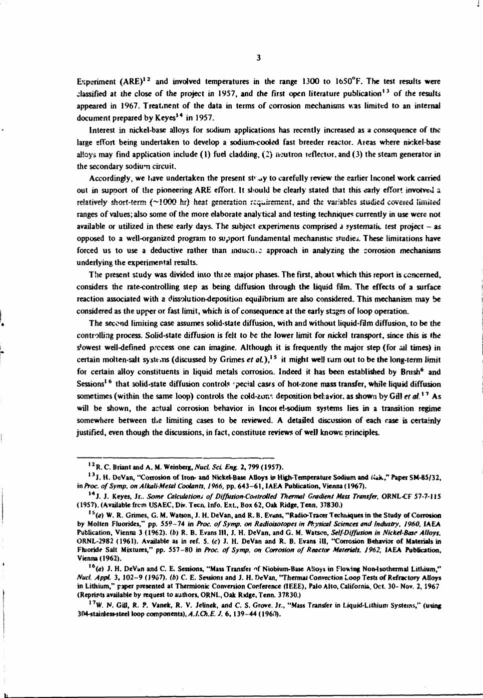
Liquid sodium has been utilized since 1928 with considerable success as a heat-transfer medium. An excellent review of the corrosion properties of liquid metals such as sodium was given by Epstein3 in 1955. Two years later Epstein contributed a paper4 which is now considered a classic in this field. It concerned corroaor rate equatiins with steel-mercury plus alloy steel—sodium (and NaK) systems for illustrative purposes. For stainless steels, reactions of iron and sodium with oxygen and related contaminating compounds were summarized in terms of four serial reactions, most products and reactants of which canceled out to yield

Fe(s)^FeOO, (la)

where 5 and d represent, respectively, the solid and dissolved species. As compared with the diffusion-limited case, that is, flow limited F~y mass-transfer liquid-film coefficients, the reaction-rate correlation gave the best agreement with experimental sodium corrosion results. Thus the reaction-rate mechanism was favored by this comparison.

We should note here that a liquid-film coefficient and a first-order reaction rate combined correctly impart the same influence on the final results.Therefore, if the controlling reaction cannot be definitely specified the only v/ay to separate the relative contributions of film and reaction effects in positive fashion

'On loan from the Reactor Chemistry Division. 2 Mathematics Division. 3L. F. Epstein, "Corrosion by Liquid Metals," Proc. Intern. Conf. Peaceful Uses At. Energy, Geneva 9. 311-17 (1956). 4 L. F. Epstein, "Static and Dynamic Corrosion and Mass Transfer in Liquid Metal Systems," Chem. Eng. Progr.. Symp.

Ser. 20 53,67-81(1956).

1

££B3£«£ie8aWGB* , %!3^-22£5£tf&J83*lb»fr . «r- t- f---'-- » * " r^r^-'**^^' _*- ' - ' i fci .^-

BLANK PAGE

2

is to vary the Reynolds number, holding everything else constant. Farther nore, to detect solid-state diffusion effects, one should study corrosion <ts a function of time - preferably over a series of fixed conditions such as constant Reynolds numbers or unaltered temperature profiles.

To digress further, it should be mentioned that the liquid sodium-stainless steel programs have enjoyed an unusually long tenure of financial support and worldwide technical interest. This has come about becau J these materials were »£Cu as structural and fuel cladding materials in "first-generaHOP." fast breeder reactors as envisioned (with minor variations) in several countries. Accordingly there have been numerous progress reports, topical reports, and publications on the corrosion behavior of sodium-stiinlcaa »;eel systems. Significant among these is a report by Mottley5 wherein a special sort of liquid-diffusion filn. for FeO dissolution is introduced. This report is particularly enhanced by a special preface authored by Epstein, who dearly outlines the implications of Mcttley's work and mentions the unusual variety of available sombility data. Additional results of interest are presented by Brush.6 who demonstrates the concentration complexities within corroded alloys; Tyzack/ who reviews sodium chemistry; Weeks et a/.,8

who also review dissolution and rates processes; and finally a simple but thorough summary by Hopenfeld and Darley.9 Other pertinent references may be obtained from the literature cited thus far.

The present report concerns the corrosion of inconel in sodium; it is oriented primarily toward nickel transport in polythermai forced-convection loops. One may wonder, therefore, why so much emphasis is placed on stainless steel researches here. There are two reasons for this: first, a tremendous amount of liquid metals research has been done with stainless steels as compared with other alloys, and second, the major components of Inconel are also present in stainless steels. Surely, at least a foundation for building a workable correlation for the Inconel results can be gained from a perusal of the steel reports, since many of these are quite general in nature and are based on acceptable (noncontroversial) methods. Also many of the experimental difficulties and seemingly unusual experimental results are common to both the Inconel and the stainless steel systems. The basic difference between the two is the relative insensitivity of Inconel corrosion to oxygen contamination as compared with the rather marked oxygen sensitivity exhibited by the stainless steel system. * °»' *

Corrosion tests of nickel-base alloys, particularly inconel, were conducted at ORNL from about 1948 to 1957. The tests were aimed toward qualifying sodium as a heat-transfer fluid in the Aircraft Reactor

5 J. D. Mottley, Sodium Mass Transfer. VII. Corrosion of Stainless Sted in Isothermal Regions of a Flowing Sodium System, GEAP-4313 (February 1964). (Available from Clearinghouse for Technical Information, NBS, U.S. Dept. Commerce, Springfield, Va. 22151.)

*E. G. Brush, Sodium Mass Transfer. XVI. The Selective Corrosion, Component of Steel Exposed to Flowing Sodium, GEAP-4832 (March 1965). Availability as in ref. 5.

7C. Tyzack, "Application of Sodium Chemistiy in Fast Nuclear Reactors," Chem. Soc. ILondon) Spec. PuN. 22, 236-59(1966).

8J. R. Weeks, C. J. Klamut, and D. H. Gurinsky, "Corrosion by Alloy Metals," IAEA Paper SM-8S/40 presented at Alkali-Metal Coolants Symposium (Vienna, Austria, November 28 to December 2. 1966). Also issued as BNL-10800 (1966). Availability as in ref. 5.

9 J. Hopenfeld and D. Dariey, Dynamic Mass Transfer of Stainless Steel in Sodium Under High-Heat-Flux Conditions, NAA-SR-12447 (July 1967). Availability as in ref. 5.

I °N. P. Agapova, A. G. Ioltukhovsky, and V. V. Komaneev, "Behavior of Stainless Steel in Sodium in the 600-900°C Temperature Region," Paper SM-85/151 in Proc. of Symp. Alkali-Metal Coolants, 1966, pp. 85-96, IAEA Publication, Vienna (19t 7).

I I (*) A. W. Thorley and C. Tyzack, 'The Corrosion Behavior of Iron and Nickel-Based AUoyj in High-Temperature Sodium," UK.AEA Document TRG Report 1356(c) (October 1966). (Available from UKAEA installation at Cukheth, England.) (b} A somewhat different version of this manuscript appears as: Paper SM-85/118 in Proc. of Symp. on Alkali-Metal Coolants, J966, pp. 97-118, IAEA Publication, Vienna (1967).

3

Experiment (ARE) 1 2 and involved temperatures in the range 1300 to 1650°F. The test results were classified at the close of the project in 1957, and the first open literature publication1 3 of the results appeared in 1967. Treatment of the data in terms of corrosion mechanisms vras limited to an internal document prepared by Keyes 1 4 in 1957.

Interest in nickel-base alloys for sodium applications has recently increased as a consequence of the large effort being undertaken to develop a sodium-cooled fast breeder reactor. Aieas where nickel-base alloys may find application include (1) fuel cladding, (2) neutron reflector, and (3) the steam generator in the secondary sodium circuit.

Accordingly, we have undertaken the present st' ^y to carefully review the earlier Inconel work carried out in support of the pioneering ARE effort. It should be clearly stated that this early effort involved a. relatively short-term (~!000 hr) heat generation requirement, and the variables studied covered limited ranges of values; also some of the more elaborate analytical and testing techniques currently in use were not available or utilized in these early days. The subject experiments comprised a systematic test project - as opposed to a well-organized program to support fundamental mechanistic studies. These limitations have forced us to use a deductive rather than mducti.j approach in analyzing the corrosion mechanisms underlying the experimental results.

The present study was divided into three major phases. The first, about which this report is concerned, considers the rate-controlling step as being diffusion through the liquid film. The effects of a surface reaction associated with a dissolution-deposition equilibrium are also considered. This mechanism may be considered as the upper or fast limit, which is of consequence at the early stages of loop operation.

The second limiting case assumes solid-state diffusion, with and without liquid-film diffusion, to be the controlling process. Solid-state diffusion is felt to be the lower limit for nickel transport, since this is the s'owest well-defined process one can imagine. Although it is frequently the major step (for ail times) in certain molten-salt systems (discussed by Grimes et at)} 5 it might well rum out to be the long-term limit for certain alloy constituents in liquid metals corrosion. Indeed it has been established by Brush6 and Sessions1 6 that solid-state diffusion controls -pedal cases of hot-zone mass transfer, while liquid diffusion sometimes (within the same loop) controls the cold-zon* deposition behavior, as shown by Gill el al'7 As will be shown, the actual corrosion behavior in Incoi e!-sodium systems lies in a transition regime somewhere between the limiting cases to be reviewed. A detailed discussion of each rase is certainly justified, even though the discussions, in fact, constitute reviews of well known principles.

1 2 R. C. Briant and A. M. Weinberg, Nucl. Set Eng. 2, 799 (1957). 1 3 J. H. DeVan, "Corrosion of Iron- and Nickel-Base Alloys in High-Temperature Sodium and Nik," Paper SM-85/32,

in Proc. ofSymp. on Alkali-Metal Coolants, 1966, pp. 643-61, IAEA Publication, Vienna (1967). 1 4 J. J. Keyes, Jr.. Some Calculation* of Diffusion-Controlled Thermal Gradient Mats Transfer, ORNL-CF 57-7-115

(1957). (Available from USAEC, Div. Teen. Info. ExL, Box 62, Oak Ridge, Tenn. 37830.) 1 5(«) W. R. Grimes, G. M. Watson, J. H. DeVan, and R. B. Evans, "Radio-Tracer Techniques in the Study of Corrosion

by Molten Fluorides," pp. 559-74 in Proc. of Symp. on Radioisotopes in Physical Sciences and Industry, I960, IAEA Publication, Vienna 3 (1962). (b) R. B. Evans III, J. H. DeVan, and G. M. Watson, Self-Diffusion in Nickel-Base Alloys, ORNL-2982 (1961). Available as in ref. 5. (c) J. H. DeVan and R. B. Evans ill, "Corrosion Behavior of Materials in Fluoride Salt Mixtures," pp. 557-80 in Proc. of Symp. on Corrosion of Reactor Materials, J962, IAEA Publication, Vienna (1962).

1 6 (A) J. H. DeVan and C. E. Sessions, "Mass Transfet "f Niobium-Base AUoys in Flowing Non-Isothermal Lithium," Nucl. Appl. 3, 102-9 (J 967). (b) C. E. Sessions and J. H. DeVan, 'Thermal Convection Loop Tests of Refractory AUoys in Lithium," paper presented at Thermionic Conversion Conference (IEEE), Palo Alto, California., Oct 30- Nov. 2, 1967 (Reprints available by request to authors, ORNL, Oak Ridge, Tenn. 37830.)

17W. N. Gill, R. ?. Vanek, R. V. Jelinek, and C. S. Grove. Jr., "Mass Transfer in Liquid-Lithium Systems," (using 304-stainless-steel loop components), A.I.Ch.E. J. 6,139-44 (196(1).

4

As an alternative to these idealized limiting cases,1 8 one might consider correlating the experiment! inconel dsta by an empirical approach that combiner all the individual mechanisms. The results, at best, would be of the form of an approximate formula which allowed only short-range interpolations from the "base conditions" at which the majority of the lncc?:el experiments were conducted.

*M

A.

D

e f

fx fi

fm g h ti_ h H i

k k'

* 1

kexp

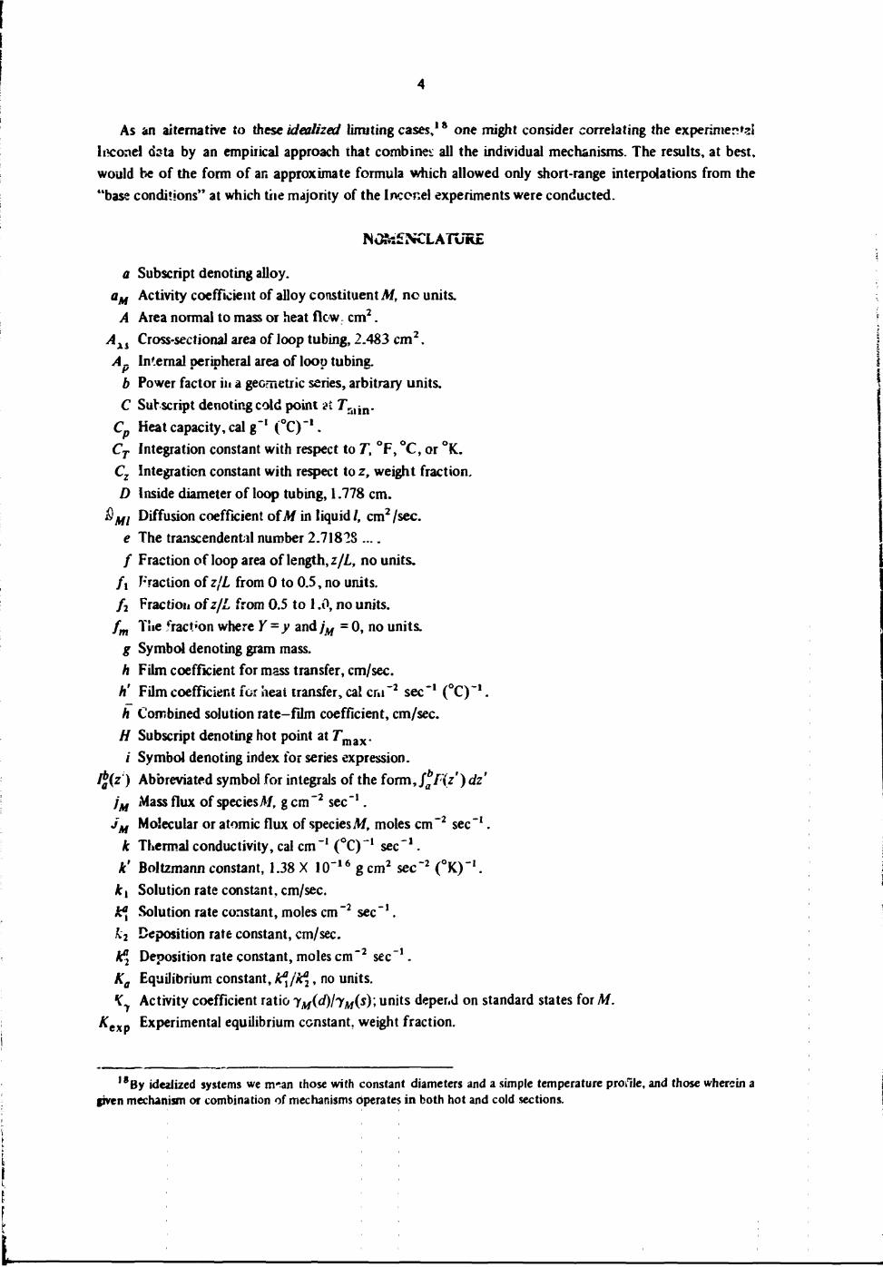
NOMENCLATURE

Subscript denoting alloy. Activity coefficient of alloy constituent M, no units. Area normal to mass or heat flew cm 2. Cross-sectional area of loop tubing, 2.483 cm 2 . Internal peripheral area of loop tubing. Power factor in a geometric series, arbitrary units. Sut script denoting cold point at 7\. t l i n. Heat capacity, cal g"1 (°C) _ 1 . Integration constant with respect to T, °F, °C, or °K. Integration constant with respect to z, weight fraction. Inside diameter of loop tubing, 1.778 cm. Diffusion coefficient ofM in liquid/, cm2/sec. The transcendental number 2.71828 .... Fraction of loop area of length, z/L, no units. Fraction of z/L from 0 to 0.5, no units. Fraction of z/L from 0.5 to 1.0, no units. The fraction where Y=y and/M = 0, no units. Symbol denoting gram mass. Film coefficient for mass transfer, cm/sec. Film coefficient for heat transfer, cal cm - 2 sec"1 (°C)~1. Combined solution rate-film coefficient, cm/sec. Subscript denoting hot point at r m a x . Symbol denoting index for series expression. Abbreviated symbol for integrals of the form,/*/'*(?') dz Mass flux of species M, g e m - 2 sec"1. Molecular or atomic flux of speciesM, moles cm"2 sec"1.

>-i - i Thermal conductivity, cal cm _ 1 (°C) * sec Boltzmannconstant, 1.38 X 10" 1 6 gem 2 sec - 2 (°K) _ 1 . Solution rate constant, cm/sec. Solution rate constant, moles cm"2 sec - 1 . Deposition rate constant, cm/sec. Deposition rate constant, moles cm"2 sec - 1 . Equilibrium constant, k\/k\, no units. Activity coefficient ratio lM(d)lyM{s)\ units deper.d on standard states for M. Experimental equilibrium constant, weight fraction.

1 8 By idealized systems we m-an those with constant diameters and a simple temperature profile, and those wherein a given mechanism or combination of mechanisms Operates in both hot and cold sections.

5

/ Subscript denoting liquid metal. L Total loop 1« ngth, 905.6 cm. m Molecular or atomic weight, g/mole. M Subscript denoting metal constituent.

A/(s) Symbol denoting metal constituent in solid solution. M(d) Symbol denoting metal constituent in liquid solutior.

n Number of completed cycles, no units. iV N u Nusselt number for mass or heat transfer, respectively, tiD/$Mi o r *'£/*/» n o units. NpT Prandtl number, Cpn/kj, no units.

^Re Reynolds number, Dvp/n, no units. NSc Schmidt number, n/pDMi, no units.

q Constant group a/v oi fi/L, cm -*. Q Volumetric liquid flow rate in loop at <D, cm3/sec.

rM Atomic radius of M diffusing in liquid, cm. / Time, sec. f Transformed time variable, t - z/v, sec. T Temperature of bulk liquid, °F, °C, or °K.

<D Arithmetic average temperature, ( ^ X ^ H + ^c)> u n * t s a^ove. u Arbitrary variable, no units. U Overall heat transfer coefficient, cal c m - 2 sec - 1 . v Liquid flow velocity, Q/Axs, 63.6 cm/sec. x Mole fraction of M in alloy, no units. v Weight fraction of M in bulk liquid, no units.

y0 Initial concentration of solute M in liquid, no units. v Mole fraction of M in liquid, no units.

y* Weight fraction of M in liquid at interface, no units. Y Weight fraction of A/ in liquid when saturated, no units.

<y> Arithmetic average of Y, (V 2XJ'H + ^c)» n o U f U t s -Ymm Saturation value of M a t / m (not Yc at Tc), no units.

z Linear flow coordinate for v or Q, cm. z 0 Position of a fluid element at z and t at time zero, z 0 = nL + z - vt, cm. z Transformed position variable, cm. « Constant group, 4h/D, sec"1. a Constant group, hnDL/Q, no units. /?' Constant group, UnDL/QpjCp, no units. 7 Activity coefficient, units selected to makea^ dimensionless. A Symbol to denote temperature or concentration drop (e.g., AT=TH - Tc). H Viscosity coefficient, g cm"1 sec - 1 . •n The transcendental number 3.1416.... p Mass density, g/cm3.

2, Symbol for sum with /' indices, r External temperature of loop wall, °F, CC, or °K.

0(f) An arbitrary constant of integration in the(z, t) coordinate system, no units. \j/(t) An alternate expression for introduv-ing>'(0, t), no units.

6

TEMPERATURE PROFILES AND LOOP CONFIGURATIONS

Reference and Prototype Loops

Our ultimate goal is to develop a general solution for a variety of loops having arbitrary temperature profiles along z, which denotes some distance along the loop measured from a convenient referent? point. The solution can be given in terms of quadratures (areas) for an arbitrary temperature profile. In order to evaluate these quadratures, it is frequently convenient to approximate the temperature profile by several straight-line segments. A typical pump-loop configuration and profile shall be considered to inject realism; this will be called the reference loop. Next we shall consider very simple loops designed to possess a fair degree of equivalence to the reference loop. These will be called the prototype loops. Simple, and sometimes symmetrical, prototypes are desirable io ease the burden associated with the mathematics, as it might affect our method of presentation.

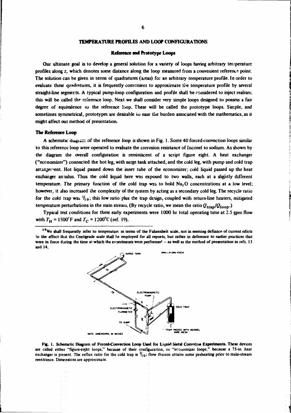
The Reference Loop A schematic dugiir.". of the reference loop is shown in Fig. 1. Some 40 forced-convection loops similar

to this reference loop were operated to evaluate the corrosion resistance of Inconel to sodium. As shown by the diagram the overall configuration is reminiscent of a script figure eight. A heat exchanger ("economizer") connected the hot leg, with surge tank attached, and the cold leg, with pump and cold trap arrangement. Hot liquid passed down the inner tube of the economizer; cold liquid passed up the heat exchanger aniulus. Thus the cold liquid here was exposed to two walls, each at a slightly different temperature. The primary function of the cold trap W2s to hold Na 2 0 concentrations at a low level; however, it also increased the complexity of the system by acting as a secondary cold leg. The recycle ratio for the cold trap was % 0 ; this low ratio plus the trap design, coupled with return-line heaters, mitigated temperature perturbations in the main stream. (By recycle ratio, we mean the ratio (?trap/£?loop-)

Typical test conditions for these early experiments were 1000 hr total operating time at 2.S gpm flow with TH = 1500CF and Tc = 1200°C (ref. 19).

I 9 i We shall frequently refer to temperature in terms of the Fahrenheit scale, not in seeming defiance of current edicts to the effect Out the Centigrade scale shall t« employed for all reports, but rather in deference to earlier practices that were in force during the time at which the experiments were performed - as well as the method of presentation in refs. 13 and 14.

SURGE TANK omaL-'-K-oae e » ! «

COLO TRAP

NOTE - OMENSKWS m M C H C S

TRAP PACKED WITH MCONEL •IRE MESH

Fig. 1. Schematic Diagram of Forced-Convection Loop Used for Liqukt Metal Corrosion Experiments. These devices are called either "figure-eight loops," because of their configuration, or "economizer loops," because a 75-in. heat exchanger is present. The reflux ratio for the cold trap is V, 0; flow thetein attains some preheating prior to main-stream reentrance. Dimensions are approximate.

/

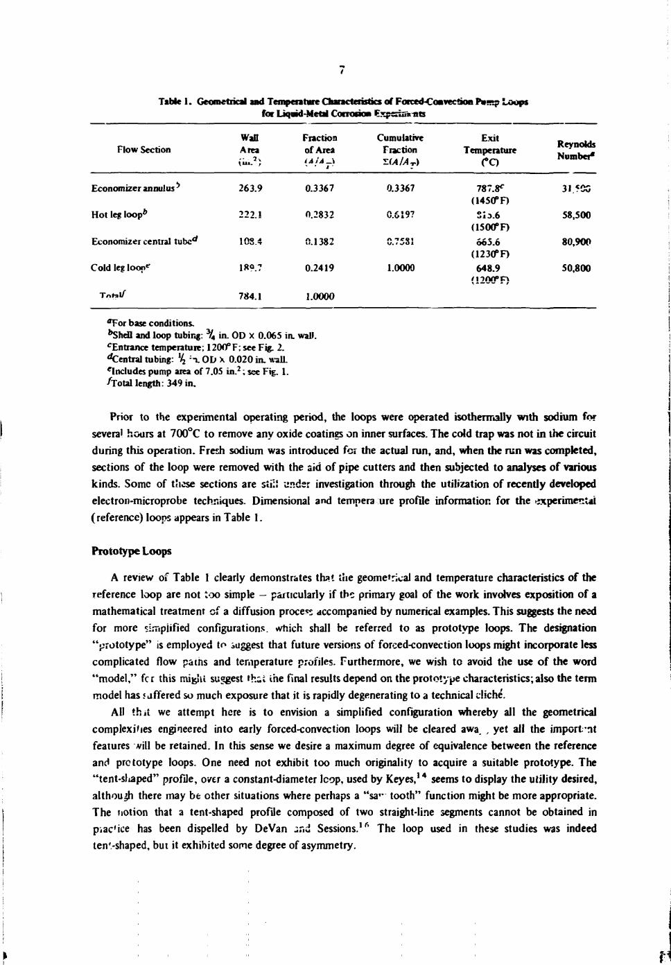
Table 1. Geometrical and Temperature Characteristics of Forced-Coavection fmrnp Loops for Liquid-Metal Cocrotkw Expsnosnts

Wall Fraction Cumulative Exit Reynolds Number*

Flow Section Area -- 2v

of Area ' • l •

Fraction •LlAlAr)

Temperature (°C)

Reynolds Number*

Economizer annulus -* 263.9 0.3367 0.3367 787.8* (1450°F)

31.5CG

Hot leg loop* 222.1 0.2832 0.6197 So .6 (1500° F)

58,500

Economizer central tube** 103.4 0.1382 665.6 (1230° F)

80,900

Cold leg loon* 189.7 0.2419 1.0000 648.9 \ * — W W • f

50,800

Total/" 784.1 1.0000

*For base conditions. *Shell and loop tubing: % in. OD x 0.065 in. wall. cEntrance temperature; 1200°F; see Fig. 2. Central tubing: \ ~x OD X 0.020 in. wall, includes pump area of 7.05 in.2; see Fig. 1. total length: 349 in.

Prior to the experimental operating period, the loops were operated isothermally with sodium for several hours at 700°C to remove any oxide coatings on inner surfaces. The cold trap was not in the circuit during this operation. Fresh sodium was introduced for the actual run, and, when the run was completed, sections of the loop were removed with the aid of pipe cutters and then subjected to analyses of various kinds. Some of these sections are still under investigation through the utilization of recently developed electron-microprobe techniques. Dimensional and tempera ure profile information for the sxperimeniai (reference) loops appears in Table 1.

Prototype Loops

A review of Table 1 clearly demonstrates that the geometrical and temperature characteristics of the reference loop are not too simple - particularly if the primary goal of the work involves exposition of a mathematical treatment of a diffusion process accompanied by numerical examples. This suggests the need for more simplified configurations vrtiich shall be referred to as prototype loops. The designation "prototype" is employed to suggest that future versions of forced-convection loops might incorporate less complicated flow paths and temperature profiles. Furthermore, we wish to avoid the use of the word "model," fcr this might suggest thsi ihe final results depend on the prototype characteristics; also the term model has 5 jffered so much exposure that it is rapidly degenerating to a technical cliche.

All th it we attempt here is to envision a simplified configuration whereby all the geometrical complexities engineered into early forced-convection loops will be cleared awa. , yet all the import'tit features vill be retained. In this sense we desire a maximum degree of equivalence between the reference and prototype loops. One need not exhibit too much originality to acquire a suitable prototype. The "tent-sliaped" profile, over a constant-diameter lcop, used by Keyes, 1 4 seems to display the utility desired, although there may be other situations where perhaps a "sa'~ tooth" function might be more appropriate. The notion that a tent-shaped profile composed of two straight-line segments cannot be obtained in piac'ice has been dispelled by DeVan and Sessions.1 6 The loop used in these studies was indeed ten'.-shaped, but it exhibited some degree of asymmetry.

8

We shall eventually establish that bquRMim diffusion did not control mass-transfer kinetics in the subject Incond pcmp-loop experiments; thus the major consideration is acquisition of a prototype loop with an area equivalent to the reference loop. In Table 1 one finds that the total area exposed to the liquid is 784.1 in. 2 , or 1991 cm 2 . If the diameter is assumed to be constant at 0.70 in. all around the loop, its total length will be 905.6 cm, which is not too far removed from the actual value of 349 in. (886 cm) for the reference loop. The average / V R e weighted according to the fractional areas involved K 5.06 X i ( r .

It seems reasonable to inquire as to the </VRe> for the prototype. Based on D, ^ N ^ N , , ty p / ? and nt

values, which are, respectively, 0.89 cm, 3.3 X 10" 4 cm 2/sec, 63.5 cm/sec, 0.772 g/cm 3, and 1.80 X 10" 3 g c m - 1 s ec ' 1 , one may compute the h as well as the A / R e using

* N u = 7 (0 .023 )^? XA/f;; . 33

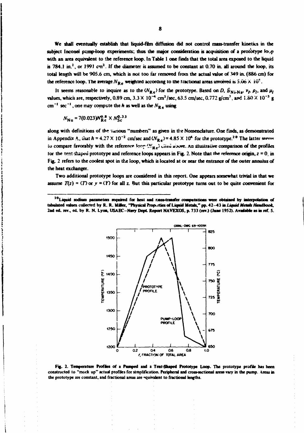
along with definitions of th? v«nous "numbers" as given in the Nomenclature. One finds, as demonstrated in Appendix A, ihat h - 4.27 X 10" 2 cm/sec andCVR e>=4.85 X 10* for the prototype. 2 0 The latter «««« to compare favorably with the reference w>~ <-VRe) dtcu «;jove. An illustrative comparison of the profiles tor the tent shaped prototype and reference loops appears in Fig. 2. Note that the reference origin, z - 0. in Fig. 2 refers to the coolest spot in the loop, which is located at or near the entrance of the outer annutus of the heat exchanger.

Two additional prototype loops are considered in this report. One appears somewhat trivial in that we assume J\z) = iT) or y - iY) for all z. But this particular prototype turns out to be quite convenient for

20, Liquid sodium parameters required for heat aad rjass-trausfer computations were obtaaed by nterpoUriou of tabulated values collected by R. R. Mater, "Physical Prop*/ties of Liquid Metals," pp. 42-43 » Liquid Hefh Handbook. 2nd ed. rev„ ed. by R. N. Lyon, USA£C-Navy DepL Report NAVEXOS, p. 733 (rev.) (June 1952). Avafabte as in ret S.

OWN- OWC 69-tCOSi

150C -

1450 -

£ 1400 -

T

/PROTOTYPE 'PROFILE

PU*P-L00P PROFILE

- 825

800

- 775

04 06 f, FRACTION OF TOTAL AREA

Fig. 2. Temperature Profiles of a Pumped and a Tent-Shaped Prototype Loop. The prototype profile has been constructed to "mock up" actual profiles for simplification. Peripheral and cross-sectional areas vary in the pump. Areas in the prototype are constant, and fractional areas are equivalent to fractional lengths.

9

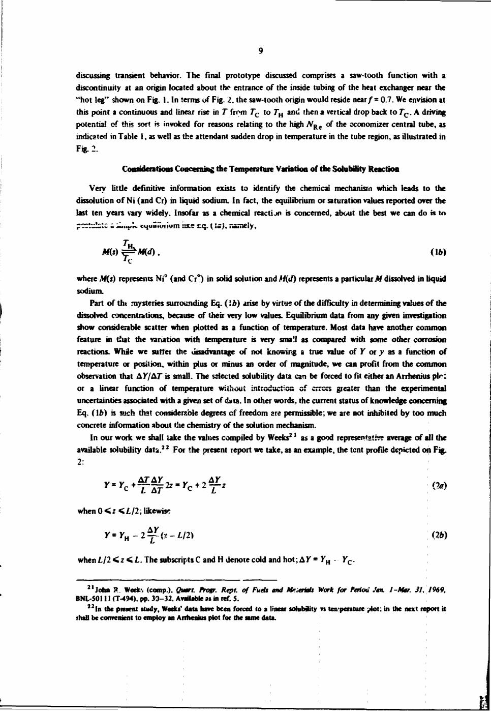
discussing transient behavior. The final prototype discussed comprises a saw-tooth function with a discontinuity at an origin located about the entrance of the inside tubing of the heat exchanger near the "hot leg" shown on Fig. 1. In terms of Fig. 2, the saw-tooth origin would reside near/= 0.7. We envision at this point a continuous and linear rise in T from 7*c to TH and then a vertical drop back to 7*c. A driving potential of this sort * invoked for reasons relating to the high vVRe of the economizer central tube, as indicated in Table 1, as well as the attendant sudden drop in temperature in the tube region, as illustrated in Fig. 2.

Considerations Concerning die Temperature Variation of die Solubffity Reaction

Very little definitive information exists to identify the chemical mechanism which leads to the dissolution of Ni (and Cr) in liquid sodium. In fact, the equilibrium or saturation values reported over the last ten years vary widely. Insofar as a chemical reaction is concerned, about the best we can do is to pcrtu! :c i ^...K!v c^uiitvuum u&£ tq. {.:-), namely,

T M(s) ^=±AK<f). (16)

where M(s) represents Ni° (and Cr°) in solid solution and H(d) represents a particular M dissolved in liquid sodium.

Part of tilt mysteries surrounding Eq. (lb) arise by virtue of die difficulty in determining values of the dissolved concentrations, because of their very low values. Equilibrium data from any given investigation show considerable scatter when plotted as a function of temperature. Most data have another common feature in that the variation with temperature is very sma'J as compared with some other corrosion reactions. Whie we suffer the disadvantage of not knowing a true value of Y or v as a function of temperature or position, within plus or minus an order of magnitude, we can profit from die common observation that A Y/&T is small. The selected solubility data can be forced to fit either an Arrhenius plct or a linear function of temperature without introduction of errors greater than die experimental uncertainties associated with a given set of data. In other words, the current status of knowledge concerning Eq. (16) is such that considerable degrees cf freedom are permissible; we are not inhibited by too much concrete information about the chemistry of die solution mechanism.

In our work we shall take die values compiled by Weeks3' as a good representative average of all die available solubility data.2 3 For the present report we take, as an example, die tent profile depicted on Fig. 2:

when 0 <z <L/2; likewise

y=YH -2~{t-LI2\ (2b)

when L/2 < z < L. The subscripts C and H denote cold and hot; AY * YH - Yc.

3'John R. Week', (comp.). Quart. Progr. Rept. of Fuels and M*.trials Work for Period Jon. J-Mar. SI, 1969, BNL-50111 (T-494), pp. 30-32. Available «in ref. 5.

3 3In the present study, Weeks' data have been forced to a linear sohibiity vs ten'penture plot; in the next report it fhall be convenient to employ an Arrheniiis plot for the same data.

10

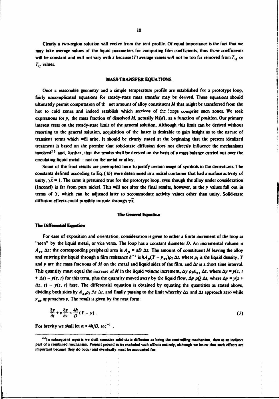
Clearly a two-region solution will evolve from the tent profile. Of equal importance is the fact that we may take average values of the liquid parameters for computing film coefficients; thus tbvse coefficients will be constant and will not vary with z because<D average values will not be too far removed from TH or Tc values.

MASS-TRANSFER EQUATIONS

Once a reasonable geometry and a simple temperature profile are established for a prototype loop, fairly uncomplicated equations for steady-state mass transfer may be derived. These equations should ultimately permit computation of th net amount of alloy constituent M that might be transferred from the hot to cold zones and indeed establish which section* of the !ccp£ comprise such zones. We seek expressions for y, the mass fraction of dissolved M, actually NiV), as a function of position. Our primary interest rests on the steady-state limit of the general solution. Although this limit can be derived without resorting to the general solution, acquisition of the latter is desirable to gain insight as to the nature of transient terms which will arise. It shouid be clearly stated at the beginning that the present idealized treatment is based on the premise that solid-state diffusion does not directly influence the mechanisms involved2 3 and, further, that the results shall be derived on the basis of a mass balance carried out over the circulating liquid metal - not on the metal or alloy.

Some of the final results are preempted here to justify certain usage of symbols in the derivations. The constants defined according to Eq. (\b) were determined in a nickel container that had a surface activity of unity, yx = 1. The same is presumed true for the prototype loop, even though the alloy under consideration (Inconel) is far from pure nickel. This will not alter the final results, however, as the y values fall out in terms of Y, which can be adjusted later to accommodate activity values other than unity. Solid-state diffusion effects could possibly intrude through yx.

The General Equation

The Differential Equation

For ease of exposition and orientation, consideration is given to either a finite increment of the loop as "seen" by the liquid metal, or vice versa. The loop has a constant diameter D. An incremental volume is Axs Az; the conesponding peripheral area \&Ap-nDAz. The amount of constituent M leaving the alloy and entering the liquid through a film resistance h "' is hAp(Y - y„)pj Ar, where pl is the liquid density, Y and y are the mass fractions of M on the metal and liquid sides of the film, and A/ is a short time interval. This quantity must equal the increase of M in the iiquid volume increment, Ay PjAxx Az, where Ay sy(z, t + A/) -y{z, t) for this term, phis the quantity moved away by the liquid flow, Ay pQ Ar, where Ay -y\z + Az> 0 - y(z> ' ) kete. The differential equation is obtained by equating the quantities as stated above, dividing both sides by Axspt Az A/, and finally passing to the limit whereby Ax and A/ approach zero while ytM approaches jr. The result is given by the neat form:

bt Bz DU y r ( 3 )

For brevity we shall let a - 4h/D, sec"' .

2 JIn subsequent reports we shall consider sotid-ttate diffusion as being the controlling mechanism, then as an indirect part of a combined mechanism. Present ground rules excluded wch effects entirely, although we know that such effects ate important because they do occur and eventually must be accounted for.

11

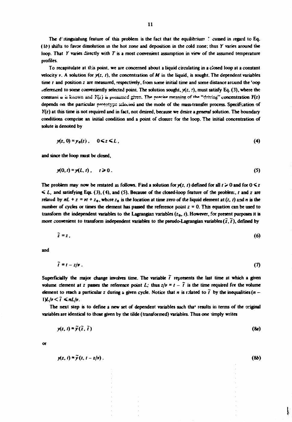
The d:>tinguishing feature of this problem is the fact that the equilibrium ! cussed in regard to Eq. (lb) shifts to favor dissolution in the hot zone and deposition in the cold zone; thus Y varies around the loop. That Y varies directly with T is a most convenient assumption in view of the assumed temperature profiles.

To recapitulate at this point, we are concerned about a liquid circulating in a closed loop at a constant velocity v. A solution for y{z, /) , the concentration of M in the liquid, is sought. The dependent variables time / and position z are measured, respectively, from some initial time and some distance around the 'oop leferenced to some conveniently selected point. The solution sought,^,.') , must satisfy Eq. (3), where the constant u » knowT. and Y(i) b picsunwd given. Th* «««<*»«* ™»2mn* of **»* **driv;n£" concentration Y(z) depends on the particular prototype Succicd and the mode of the mass-transfer process. Specification of Y(z) at this time is not required and in fact, not desired, because we desire a general solution. The boundary conditions comprise an initial condition and a point of closure for the loop. The initial concentration of solute is denoted by

y(z,0)=yo(z), 0<z<L, (4)

and since the loop must be dosed,

M O , f ) = * I , / ) , t>0. (5)

The problem may now be restated as follows. Find a solution for y(z, i) defined for all f > 0 and for 0 < z < L, and satisfying Eqs. (3), (4), and (5). Because of the closed-loop feature of the problen:, t and z are related by nL + z - vt + z0, where z0 is the location at time zero of the liquid element at (z, t) sad n is the number of cycles or tones the element has passed the reference point z = 0. This equation can be used to transform the independent variables to the Lagrangian variables (z0, t). However, for present purposes it is more convenient to transform independent variables to the pseudo-Lagrangian variables (7, 7) , defined by

z=z, (6)

and

7 = t-z/v. (7)

Superficially the major change involves time. The variable 7 represents the last time at which a given volume dement at z passes the reference point L; thus z/v - t - 7 is the time required for the volume element to reach a particular z during a given cycle. Notice that n is related to 7 by the inequalities (/i — \)L/v<7 <nL/v.

The next step is to define a new set of dependent variables such tha* results in terms of the original variables are identical to those given by the tilde (transformed) variables. Thus one dimply writes

y(z.t)^y(i,7) (8a)

or

y{z,t)*y(zft-z/v). (%b)

12

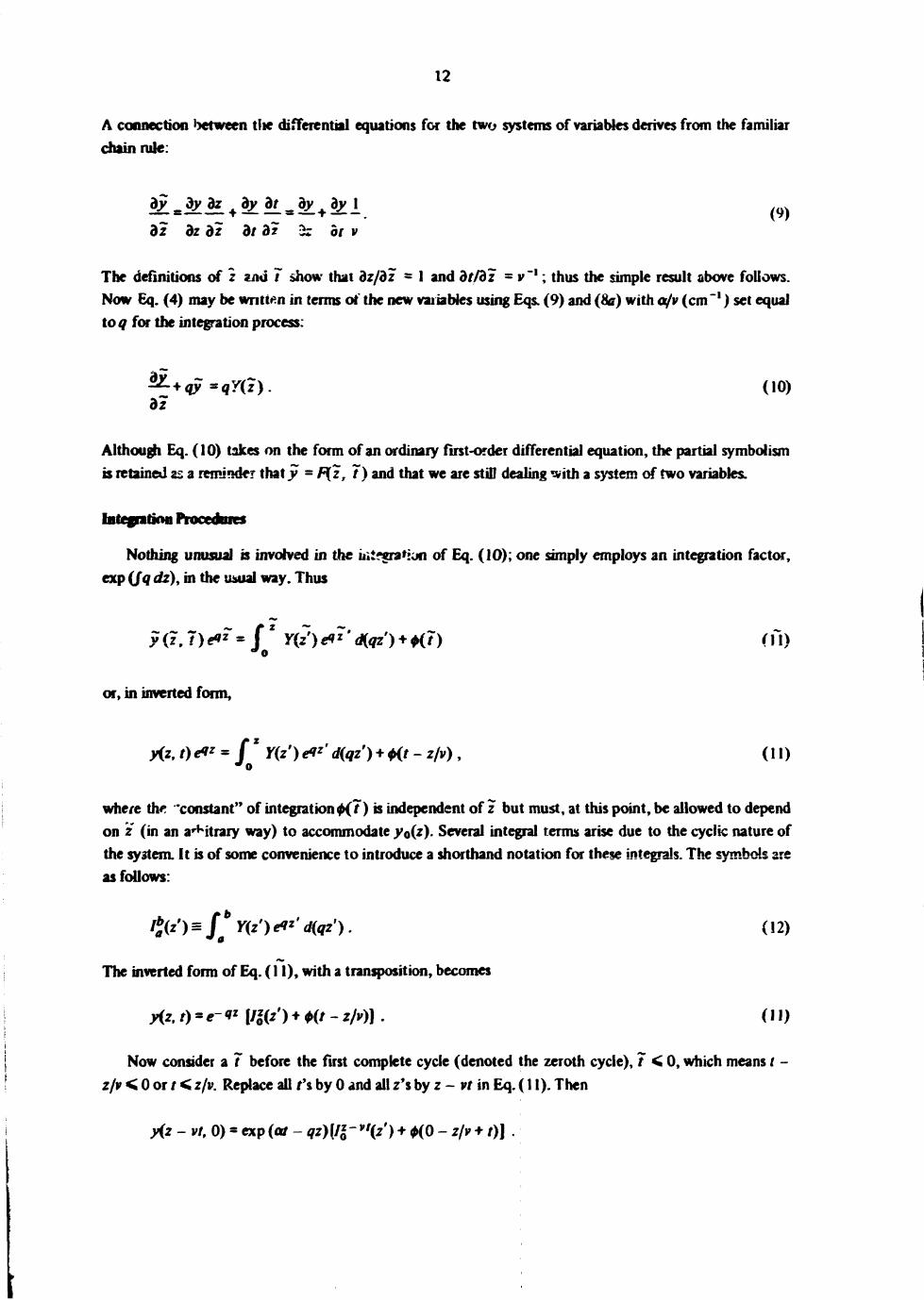
A connection between tlie differential equations for the two systems of variables derives from the familiar chain rule:

by _ by bz by bt _ dv by 1 bz bz bz bt bz 2z or v

(9)

The definitions of z and 7 show that bz/bz = 1 and df/3z = v" 1; thus the simple result above follows. Now Eq. (4) may be written in terms of the new variables using Eqs. (9) and (8c) with a/v (cm' 1) set equal to q for the integration process:

&+qy=qY(z) bz

(10)

Although Eq. (10) takes on the form of an ordinary first-order differential equation, the partial symbolism is retained as a reminder that y = F{z, 7) and that we are still dealing with a system of two variables.

Integnrjoii Procedures

Nothing unusual is involved in the u;!?era*ion of Eq. (10); one simply employs an integration factor, exp (Jq dz), in the usual way. Thus

?GJ)***(' Y{z')**'d{qz) + *(i) (11)

or, in inverted form,

yiz, t)eV = fZ Y(z') #*' d(qz') + *(/ - z/v) , (ID

where the 'constant" of integration^?) is independent of z but must, at this point, be allowed to depend on z (in an a'Htrary way) to accommodate yo(z). Several integral terms arise due to the cyclic nature of the system. It is of some convenience to introduce a shorthand notation for these integrals. The symbols are as follows:

Ib

a{z') = J*Y(z')e**'d(qz').

The inverted form of Eq. (11), with a transposition, becomes

(12)

(11)

Now consider a ? before the first complete cycle (denoted the zeroth cycle), 7 < 0, which means / z/v < 0 or / < z/v. Replace all ft by 0 and all z's by z - vt in Eq. (11). Then

y(z - K0) = exp(at - qz)[/*-vt(z') + <K0- z/v +1)) .

13

This is an equation for y0(z - w) according to the initial boundary condition [Eq. (4)]. From the above we can tind ${t - z/v) in terms of y0(z - vt) and substitute this back into Eq. (11) to obtain

y{z, 0 = e-«'.Mz - vt) + e-«*Ij_vt(z') . (13)

This applies in the time interval 0 < t < z/v. The expression for y{z, t) for / > z/v is found through evaluation of *(.' - z/v) by finding y(0, t - z/v)

using Eq. [ 11) again and feeding the result, y(0, t - z/v) ~ $(t - z/v), back into Eq. (11) again as before. Thus

y{z, t) = e~ V \y{0, t - z/v) • /|(z')J . (i4)

This applies in the time interval t > z/v, and the expression can be used to build up the working equations for all cycles including the zeroth cycle.

For times during the first complete pass,24 n - 1, recall the closure condition,

y(0,t-z/v)=y(L,t-z/v)t

then "key on" the values on the right. All z's are I and all f's are t — z/v - 7. This information is plugged into Eq. (13) to pick up the initial boundary condition,y0, from the result

y{L, t - z/v) = exp (qz - at)y0(L + z - vt) + e~«L /£„(*').

Substitution of this result back into Eq. (14), while recalling the closure condition, gives

y{z, t) = e-*'y0(L+z- vt) + e-«* [Iz

0(z') + e-«L /f + 2 _„(z')] - (15)

This equation applies for the time interval z/v < / < (I + z)/v. When t = z/v, it reverts to Eq. (13) at its upper time limit (interval); when t - (I + z)/v, it becomes an expression for they jwofile as "seen" by the volume element that resided at (z, t) = (0,0) after it has passed I (but not 2L).

An expression for the next pass is generated in the same fashion. First evaluate yiL, t - z/v) via Eq. (IS) and then substitute the results into Eq. (14):

y{z. t) =e a(y0(2l + z-vt) + e~i* [/0

?(z') + e'^ /J(z') + e~^L/^+z_„(*')]

for (L + z)/v < / < (2L + z)\v. Clearly (by induction), a general formula for n complete cycles will be

y(z. t) = e~ a 1 yJnL + z - vt) + e~ fz

n-l

'*<*')• Z i*-*L!Hz') + e-"*Li!iL.t_,fi') (16)

for [(« - 1 )L + z] jv < r < (nL + z)/v. It turns out that the argument of y0 and the lower limit of the last term is z 0 .

24By "pass" we mean a time interval Lfv occurring between cycles, ihat is, between in - \)L/v and nL/v.

14

For further discussion, consider the element whose Lagrangan coordinate z0 is zero, and the lower limit on the last integral term then becomes zero. This corresponds to singling out, as "typical," the fluid volume element which was at z = 0 at time zero. The sum of 'he series expression appearing before the second integral term becomes

t-*1 [1 - e - < " - W ] / ( i - e i l ) ;

because

( l - i / » ' * ) / ( l - u * ) , i i ' - n - l ,

is the sum 3 5 of

1 + ub + u2b • uib + ... + w"'* .

The reader may verify these results, for say n - 4, by long division. The last two integrsls may be combined through a common denominator to yield

Substitution of this result into Eq. (16) gives

y{z,t) = e-*ty0(»L + z-vt) + e-«* [/$(*')• (Lzfz~r) e^Ifa')] . (17a)

The steady-state limit \y{z, <*>)] can be derived almost by inspection if one starts at Eq. (3) and sets by/dt = 0:

yiz, ~) =y{z) =e-«* {/|(z'> + Q ] . (1&)

When z - 0, Cz becomesy(0); since

AD *M0) - e l L A0) + e-*L /i{z)

and

y(0)se -«L(\ -e«b)-ll£(z') , (19)

therefore

The series here » a geometric progression; its sum up <o the nth term appears in many handbooks and elementary textbooks.

15

andEq. (17a) is

y{z. t) = e~*!y0(nL + z-v(nL + z)!v) + y{z, «) + exp [-q(z + nL) J y(Q,«). (17*)

But q{z + nZ.) = aifiL • z)/v, and, according to our choice of limits in passing from Eq. (15) to Eq. (16), we have (nL + z) = vt; this gives us an argument of 0 fcry 0 as well as the final result below:

y(z, 0 =y(z, ~) - e ~ « 1*0, «>) - v 0(0)] . (17c)

In Eq. (17c) the steady-siate and transient parts of the solution are clearly delineated. It is easy to show that Eq. (17c) satisfies Eq. (3). A similar exercise with Eq. (16) requires more work.

transient Behavior

Discussion of transient behavior gains proper perspective only when considered in complete context describing initial operation of pump locps. In this regard one should note the usual practice of filtering and exposing reactor-grade liquid metals through and in container materials not unlike the loop alloys. It was mentioned in the section covering the reference loop that the loop was flushed, and a "fresh" batch of liquid was transferred to the loop proper and operated at isothermal conditions at <77 prior to adjustment to the AT conditions desired. Almort instantaneous adjustments, insofar as loop fluid properties are concerned, could be made in principle, ai»1 this was attempted; but. le complexities of the instrumentation and heating paraphernalia (including the trap system) made this quite difficult in practice.

Time zero for loop operation was referred to the time at which adjustments were completed. It is clear therefore that the fluid was partially equilibrated at some <D with respect to all M(d)\ dissolved components, of interest even though most of the corrosive agents were hoepfully at low levels. Although the time boundary condition for Eqs. (16) and (17) are quite general, we shall assume that jy0

= 0. This is somewhat hypothetical in nature, but it is chosen partly for reasons of mathematical tractability and also to conform with earlier treatments.14

A most reasonable transient relationship derive' from the results obtained thus far, namely Eq. (17c), over which a constant (T) and (Ware imposed. ThusX*. °°, =A®* °°) = Y(z) ~(Y\ where<Y)is %(KH + Yc). Most steady-state solutions of practical import that are encountered in this report exhibit only small variations in amplitude about <K>, for which reason the assumed function for V(J. °°) seems reasonable to us. Substitution of this information into (17c) with v 0(0) produces the form:

y/<Y>=] -txp(-at). (20)

It is interesting to note that our assumptions have led us o view the loop as a well-mixed or stirred pot operating under isothermal conditions. Precisely the same results develop when one sets 9y/3r = 0 in Eq. (3) because.? for M(d) does not change along the scream in this case. The starting point here is

dy/dt = a(m-y).

Associated boundary conditions are^0 = 0 andj' -*• (Y) as / -* °°. This leads to Eq. (20) again.

The usual procedure for asymptotic functions like this is to consider the argument corresponding to 99% equilibrium, that is, exp (-at) = 0.01, whereby a/ ~ 4.61. Based on the h value set forth in Appendix A,

16

a = 4A/i) = (4)(4.2?X |o~ 2)/l.78 =9.6 X 10": sec : ,

and clearly L/v is only 48 sec! The time for an element of volume to make a cycle around the loop is L/v = 14 sec/cyrle; thus t corresponds to roughly 3.4 cycles.

To close, one may appeal again to proper perspective and realize that experimental pump loops operate for 1000 hr on liie average. This corresponds roughly to 2.5 X JO5 cycles in the prototype loop. Consideration of transients could not be logically extended beyond ten cycles, even w^°n additional reaction rate resistances are accounted. Thus, except where solid-state diffusion is important, transient contributions are small in the average life of a loop, and the steady-state limit turns out to be the most important feature of the general solution.

STEADY-STATE SOLUTIONS

The Tent Shaped" Y(z) Function

The relationship desired is obtained by passing to the limit of very large times. Then exponential-time terms go to zero; Eq. (17c) becomes Eq. (186). Also.y(0) can be recognized via Eq. (19>. Evaluation of the integral terms defined by Eq. (12) using various definitions of Eqs. (2) yields for 0 < z <Z./2:

#>.«>*. (-$>*& 0--T) [• - (-£)!• < 2 I «> where

„_ , <*L AhL nDhL .t „ _ 0 = qL *— = — = —Q- , no umts, (22)

andforI/2<z<L.

One may obtain this result directly by setting By/dt - 0 in Eq. (3) and proceeding as in Appendix C, where more detail appears.

The Combined Form

From discussions about Tqs. < 2), it will be recalled that a complete steady-state solution involving two half-regions of L will be encountered. The task here is f.o combine or couple the two regions properly so that no discontinuities are introduced in the y profiles and so that an overall mass balance of M in the fluid is maintained. Balance information is introduced via dy/df - 0 and imposed continuity at z * 0 * L and z ~ L/2, The tact that a mass balance is attained is somewhat obscured by the required algebra; it becomes most apparent when plots of expressions for v are superposed on assumed profiles for Y.

Inspection a Eqs. (21) reveals that / * * / / . is a natural change of independent variable. The equation can be written twice, one time for each region. Over the first half we shall have/, with AY*YH- Yc and with Yc as writte- over the second half, / , . with AY2 * -AK,; this means YH replaces Yc everywhere. Both/, and/j range from 0 to 0.S; thus/*/ , in region I and/* 0.5 •*• f% in region 2. The coupling process is started by writing Eq. (2 la) for region 2 at / 2 * 0 .5 , /* I:

17

v2(0.5) =y2(0)e-("2 - AY + ( r H + 2 AY/fl(l - e"^ 2 ) . (23a)

¥ory2(0.5) on the left side, one merely writes ,(0) because at z = 0 - L, / , = 0 and/ 2 = 0.5. A similar substitution is made on the right side, since ,y2(0) =^,(0.5). However, the complete expression for^,(0.5) is used. Thus, with the aid of Eq. (2 la), Eq. (23a) becomes

^,(0)= M O ) * - * / 2 + AY f ( r c - 2 Ay//3X1 - e - * / 2 ) ] e - ^ 2 - A>'+(r H + 2 AX/0X1 - e - * / 2 ) . (236)

Tne above may be solved to yield either

j , ( 0 ) = ( l - e ~ 0 ) - i {-AY(\ - e - * / 2 ) + [Yce-»l2 -(2AYJ&)e-U2 + YH +2 Ay/0] X (1 - e " * / 2 ) }

or

^ ( 0 ) = ( l + e - ^ 2 ) - » [ (y c +2Ay/P) + ( y c - 2 A y / ^ ) e - ^ 2 ] . (24)

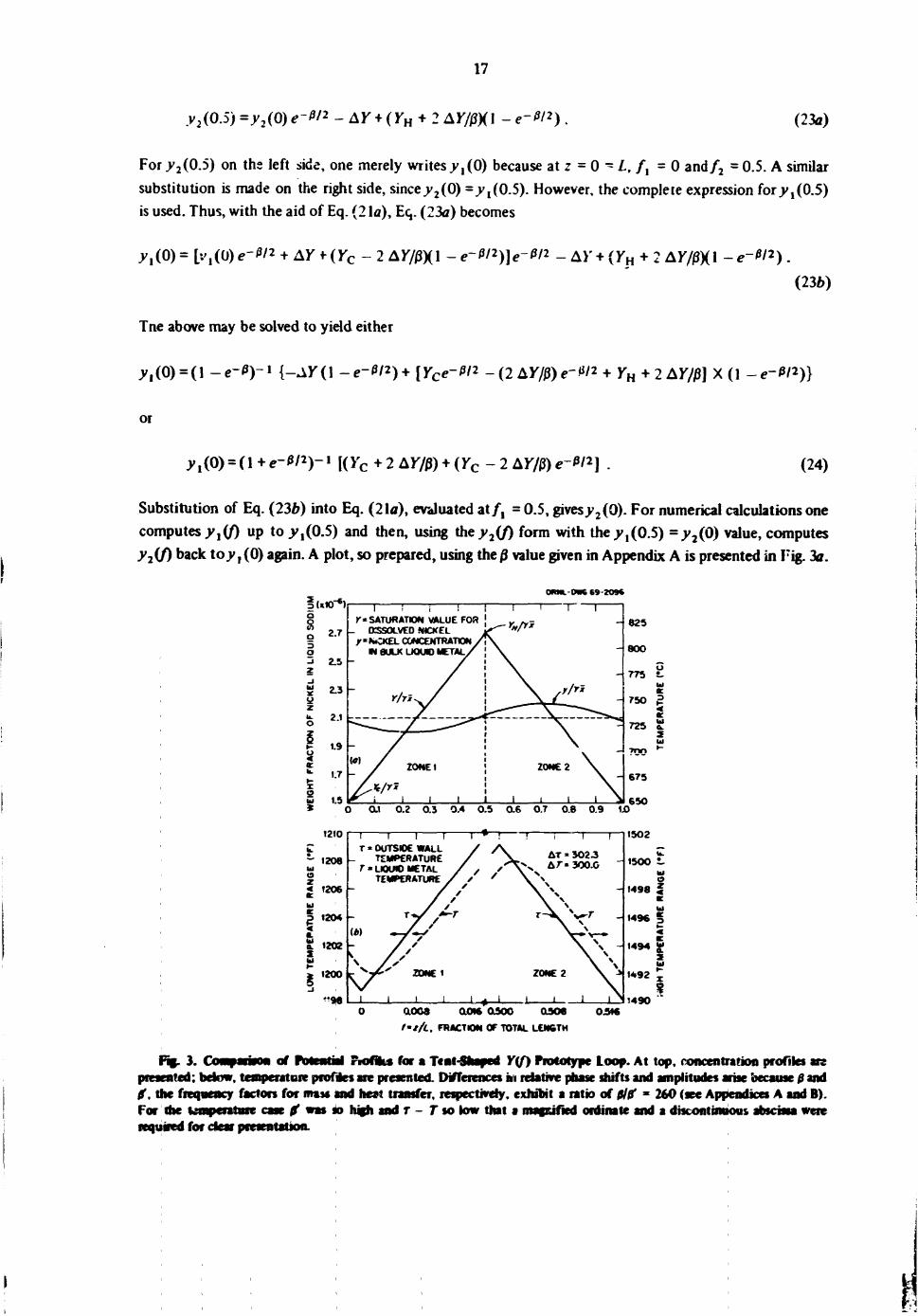
Substitution of Eq. (236) into Eq. (21a), evaluated at/, = 0.5, gives >>2(0). For numerical calculations one computes yx{f) up to ^,(0.5) and then, using they2(f) form with the^,(0.5) -y2{0) value, computes y2(f) back to.y, (0) again. A plot, so prepared, using the 0 value given in Appendix A is presented in Fig. 3a.

Q

s

ORML-INK S9-20M

9 g z

y z

2

2.7

2.5

2.3

2.1

1.9

1:7

Y* SATURATION VALUE FOR D5SOLVED NICKEL

r'KCKEL CONCENTRATION M BULK UOUO METAL

1 „ * O

1210 taT - 1208 u e | 1206 u | 1204

•. a! 1202 S

s !

ai 0.2 0.3 0.4 0.5 0.6 0.7 0.8 0.9 10 6 5 0

1200

"9«

! I ! 1 1 * ! T • OUTSlOe WALL / / V

T i l !

_ TEMPERATURE / > AT - 302.3 r«uomo METAL / • •"" V * x A7"« 300.0

TEMPERATURE / * ' \ \ / / / / • \ X / / \ \ / / \ \ - T / / r

CM m / f / / \ \

/ / / s / s \ \ \ \

>. •f"' Z0NE1 ZONE 2 \ ->

I 1 ! 1 1 A 1 1 1 1 1 s

1502

1500

1498

1496

1494

1492

1490

aoo8 aow asoo asoe t't/L, FRACTION OF TOTAL LENGTH

0516

Fig. 3. Comparison of Potential Fiofiks for a Teat-Shaped Y(f) Prototype Loop. At top, concentration profiles are presented; below, temperature profiles ate presented. Differences in relative phase shifts and amplitudes arise because fi and f, the frequency factors for mass and heat transfer, respectively, exhibit a ratio of filtf * 260 (tee Appendices A and B). For die temperature case 0 was so hsjh and T - T so low that a mafKified ordinate and a discontinuous abscissa were required for dear presentation.

18

Rehtcd Temperature Functions

A plot pertaining to the temperature profiles is presented in Fig. 36. Here, T refers to the bulk-fluid temperature. The heat-transfer behavior leading to the profile in terms of r and T is completely analogous 10 the mass-transfer behavior leading to the Y and y profiles of Fig. 3a. Marked differences in the appearance of the two profiles resulted from the selection of Scales as necessitated by dramatic differences in respective 0 values. These are 0 - 1.368 for mass transfer (Appendix A) and 0' = 356 for heat transfer (Appendix B).

The fact that the driving force functions used to describe the profiles are rehted becomes very clear when the equations in the preceding section are compared with those in Appendix C. Also, similarity of the formulas used to calculate 0 and 0' (Appendices A and B) gives additional credence to the well-known heat-and mass-transfer analogy.

!t is clear, with respect io ilic temperature plot, that external wall temperature measurements closely approximate the bulk-fluid temperature at a given point z or / . Although this statement is true mainly foi high-velocity pump loops, it is easy to accept when it is realized that T - T is much smaller than the confidence level one associates with thermocouple measurements. It is also pertinent to note here that an extra-thick wall was assumed for the prototype loop since film resistances were practically nonexistent.

Periodicity and Symmetry

The plots of Fig. 3 indicate definite periodic properties of the related function and tc a lesser extent some degrees of symmetry. All values oscillated in some fashion or other about a common mean value. As/J increases, the curve for the bulk fluid attenuates and shifts to the right with respect to the curve for the wall value. Very low/3 values tend to impart sine or cosine features to the bulk-fluid curve. Locations of the so-called "hot" and "cold" zones depend on the shift. The maximum shift approaches / = 0.25 as 0 becomes very small. Obviously the Y curve of Fig. 2a is symmetrical about/- 0.5, as originally assumed; it exhibits symmetry characteristic of an even function, Y[-(f - 0.5)] = Y\f— 0.5]. The.y curve behaves as an odd function about an/value slightly less than 0.5.

There exists another special property with respect to the y curve, but this is not at all apparent from Fig. ia. It results, in part, from the characteristics of a difference plot, namely, Y - y vs/. Individual differences are directl) proportional to the steady-state rate of transfer across any dAp at various/values. A curve of this '. ^t .an be integrated to give the positive area corresponding to the steady-state rate of mass transfer out o r the hot zone, and this must equal the negative area for the cold zone. Notice that this is simply a mass-rate balance on the wall using sign conventions adopted for the liquid balance and also that the length of both zones is /= 0.5 because 0, = 0 2 .

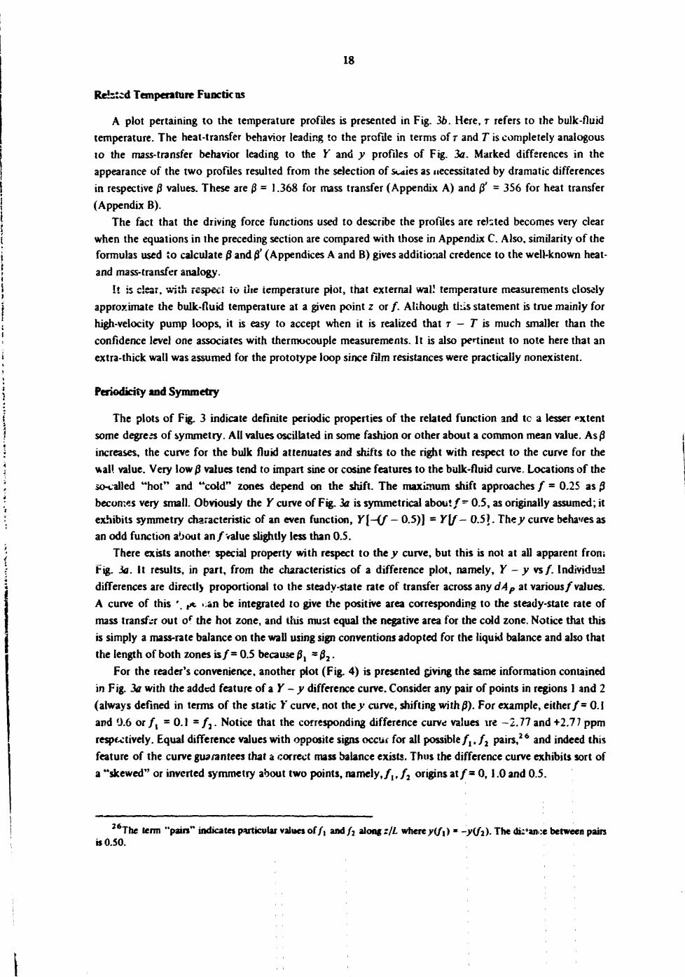
For the reader's convenience, another plot (Fig. 4) is presented giving the same information contained in Fig. 3a with the added feature ofzY-y difference curve. Consider any pair of points in regions 1 and 2 (always defined in terms of the static Y curve, not the>* curve, shifting with/?). For example, either/= 0.1 and 0.6 or/ , =0.1 = / 2 . Notice that the corresponding difference curve values ire -2.77 and+2.77 ppm respectively. Equal difference values with opposite signs occur for all possible/,,/ 2 pairs,26 and indeed this feature of the curve guarantees that a correct mass balance exists. Thus the difference curve exhibits sort of a "skewed" or inverted symmetry about two points, namely,/,, / 2 origins at /= 0,1.0 and 0.5.

The term "pain" indicates particular values of/t and/2 along;//, wherey(fi) * -is 0.50.

vC/i). The di;*anoe between pairs

19

OONL-MG 69 2093

U10~6i >U»~*)

I z o

I 3

0 0.1 0 2 0.6 0.4 0.5 0.6 a 7 0.8 0.9 1.0

f-r/L. FRACTION OF TOTAL LENGTH

Fig. 4. Fiofic of (Y - y) Couceuuaiicn Differences for a Teat-Shaped Prototype Loop, T>* upper curve in F*. 3 is superposed here as dashed lines for reference purposes. Concentrations are normalized to unit nickel activity, yx = 1. Utilization of these values for a particular alloy requires multiplication of all values by the activity applicable to the appropriate solid-solution data and corresponding standard state.

The special property of the y curve, alluded to earlier, may be demonstrated here, now that the importance of Y ~ y difference curves has been established. Consider first those values at the boundaries/= 0,1.0 and 0.5. It is desired to prove that

yAO) -YC = YH -y2(0) = r„ - yt(QS) , (25a)

or

>H+>C=.Ki(0)+.y 1 (0.5) (25b)

One may show this by operating un the right-hand side of Eq. (256) using Eq. (21a) and then Eq. (24) to eliminate tfr* factoryt(Q) [i + exp(-0/2)):

Y» • Yc =>,(0) +y,(0)e-W + AY + (Yc - 2 AY/0)(l - e"" 2)

= b,(0)(l +e-*/ 2)] + AV*(y c - 2«i7wO - e ~ p ' 2 )

= Yc + 2 AY/0 + (Yc - 2 AY/ffk-M + AY + Yc - 2 AY/0 - (YC - lAY/fa-M

= YH + YC.

The proof may be extended to all points once Eqs. (25) are validated. One m?y start with a rearranged form of Eq. (216), eliminate YH - y2(0) using Eq. (25a), and finally eliminate the remaining exponential terms with the aid of Ea. (2 la):

= [-^,(0)+r c

+ 2 AY/0\e~»f - 2 AYf* YH+2 AY/0

- 2 AY/0\e~»f- 2 AK/+ YH • 2 AY/0

s-\yl(fl)-2AY)-Yc + 2 AY/0) - 2 AK/+ K„ • 2 AK/0

- ^ • y c - J ' , ' / , ) , (26a)

20

or

YH • Yc - * ( , ' , > • Ji<C5 • / • ) • (266)

Although / = / , up to 0.5, / = / , + 0.5 beyond this point. Numerical computations are expedited by Eq. (26a).

Computation of Mass Transfer

The Exact Solution. - Attention is called to points on Fig. 4 labeled fm anc / m . , which constitute the boundaries of the hot and cold zones. These points are sometimes called "balance points" because they define areas under the Y - y difference curves that must be equal to ensure a complete overall mass balance. In terms of integrations along z or/, to obtain the subject areas,/OT and/ m . represent the limits of integration. Notice that Y-y-0ztfm = 0 and that the slope of the y curve is also zero at fm = 0, in accordance with the steady-state form of Eq. (3). All this happens because the/ and Y curves intersect one another at fm.

Acquisition of an explicit expression for fm is most desirable since its exact location will permit a computation of ym. Both are required to compute or estinute the amount of M(d) that migrates from hot to cold zones over a given time interval. Note the subscripts m and m\ which represent respectively the minimum and maximum values ofy in terms offvy. One may consider only fm in /one 1; one starts with Eq. (3), where dyfit = 0, and sets dy/df = 0:

df Q K m y m ) '

thus Ym ~ym. Note that Ym here is not YH. The next step involves substitution for Ym using Eq.(2ff), and the same for.ym using Eq. (lib). The result is

Yc + 2 AYfm * ly,(0) - Yc + 2 AY/0] e"^" • 2 &Y fm + Yc - 2 AY/0 .

Cancellation and transposition yields

6 'yW-Yc + lW

a logarithmic form of which is

fm-jK[i+ YEY~ ) • ( 2 7 )

Numerical values for the computation appear in the Nomenclature, in Fig. 4, and in Appendix A. The value of ,y ,(0) may be obtained from Eq. (24); it is 2.078. One finds that

<• - * i A , 2.078-1.500^ ^ " D o ? 1 * V* T754 J

« 0.208.

21

Of cuurse, in zone 2,

f„ > * 0.5000 • 0.208 = 0.708

Now from Eq. (3a)

ym = (1.5+ (0.208X2.4)] X 10"* - 2 . 0 X 10"

and from Eq. (12c)

•Vm'"" 10-5+2.7)-2.0] X 10~*=2.2X 10

A,i expression for ih- total mass transport again requires use of Eq. (3) with dy/bt = 0:

dy_=*DhL(Y . df Q l / y } -

Separation of varsabks and multiplication of both sides by ph the liquid metal density, gives the following integral forms for / M , the total mass flux:

/ « ' (28) p/lKrm .)-^m)]e=M pp //m'(r-^)«//.

For the time being, we shall assume that/M is constant with time; thus

Consideration of metaL other than pure Af requires that both sides of Eq. (28) be multiplied by <TX>.

In the past and perhaps based on curve shapes similar to those for temperature in Fig. 3a, it has been suggested14 that an approximate value of AM would be given by

&M'=p,[y(£) -yif[)]Q Af , (29)

where/2' and/,' would be evaluated a t / - 0.5 and/* 0, rather lhan/m , and/ m respectively. An inspection of either Fig. 3b or Fig. 4 clearly demonstrates that this is a poor approximation for the tent profile whenp* is low, because the position of fm and/O T, undergoes a nearly maximum shift whereby ,(0) -y7(0) -*• 0 at !owp\

A most interesting feature of Eq. (28) and its application is the fact that one deals with the left rather than the right side of this relationship. Thus a tedious discussion of the integration procedures required to obtain an expression for AM may be avoided hcic, since it can be shown, after considerable algfhra, that the results reduce to the simple form on the left, in other words, the integration produces a somewhat trivial identity. There are, however, many instances where the rtgtit hand side is useful; in fact, most cases encountered in this report force us to take such an approach.

' M

To amphfy the importance of the right-hand side a calculation of the total amount offi'id) transferred from hot to cold zones shall be performed for an exposure of 1000 hr. Rather than using Eq. (28) directly, it is preferable to eliminateX/"m) by the identityyifm»)+yifm) -z<K>, which follows from Eq.(266).The result is

M1 = (fil)<yxX2) MM*,) (yx)

GA/ , (30)

where <K>= '40'c + YH). Notice that <yx>has been introduced for the fust time to be consistent with Figs. 3a and 4; for Incond, y ~ 1 (assumed) and <x> = 0.738 (actual). The result, usmg values in cgs units, is

6M = (0.7725X0.738X2X1.0X iO"7Xl58X3.6X 10 6)

* 64.86 g.

Experimental results show2 7 that the total mass of nickel transported under comparable conditions could not be much greater than 12.36 g. This is about 84% of total deposits, which at most amount to 14.7 g. Thus the predicted value is roughly five times greater thwn measured values.

Approximate Fonn for Low 0. - Based on the pranise that the Y values are valid within reasonable limits of confidence, about the only means for "adjusting" the predicted value resides in considerations concerning altered values of h or yx. To consider changing yx at this point is analogous to opening Pandora's box. It shall be assumed, therefore, that kxedicted &ATs are too high because the A is too high. This can be rationalized by invoking an additional reaction-rate resistance, k^1, as discussed in Appendix D.

What is needed, then, is a good approximate fcrm for A*f when 0 is low. The exact solution becomes difficult to use for accurate results at low 0. and, furthermore, iterative techniques must be employed. Clearly, the form desired should be expli.it in h. The h and/or 0 are buried in the exact solution, sincey(f) and/ m are both transcendental functions.

At high values of 0, decreases in 0 vilues induce two effects regarding the curves of interest: first, the relative positions of the hot and cold zone shift, as discussed about Fig. 3, and second, the shape of the Y -y curve is changed from a step function [ii; which regime Eq. (29) is quite useful] v ith a minute, nearly constant Y - y value to a curve that begins 'o reflect the Y curve shape.The^ curve, on the other hand, closely approximates the Y curve when 0 is qjite large, buty(z) approximates the <Y> line when0 -* 0. AH these effects are apparent through comparisons of curves on Fig. 3.

At low values of 0, we reiterate that the Y - y curve coincides with the Y curve and that y for all practical purposes is practically a horizontal line along 00. One might suspect under such circumstances that the approximate form sought will come from the right side of Eq. (28).

A precise development of the form sought is gained by going back to Eq. (3) «nd performing a special integration at steady state for the case 0 -> 0 (i.e., dyfdf * 0). The result is a constant. It is helpful, at this point, to recall that a very high Q,2* as well as a low h, yields 0 -* 0 and that negligible M is being transferred as we pass to this limit. Thus a fluid circulating at very high Q has an ultimate, and constant,^ value of <K). The next points to consider are the location of fm and/ m . . One may recall that \nti\+u)~~u as u becomes smaii. inspection of Eq. (13) and the location of 0 therein permits

"See Fit*. 4 ,5, and 6 and Tabk IV in ref. 13. 2*We assume here that t -+k2 and the lat.er is independent of velocity.

V*

f — 1 m 0 I i fpHv,(0)-rtl

2 AK i By previous arguments. y,(0) ~ (Y}; thus fm -* % and f„. -+ % as 0 -+ 0. The average Y - y orY -<Y) ordinate over either the hot or the cold zone is obviously AYf4<yx), or A#T e x p/4. Thus

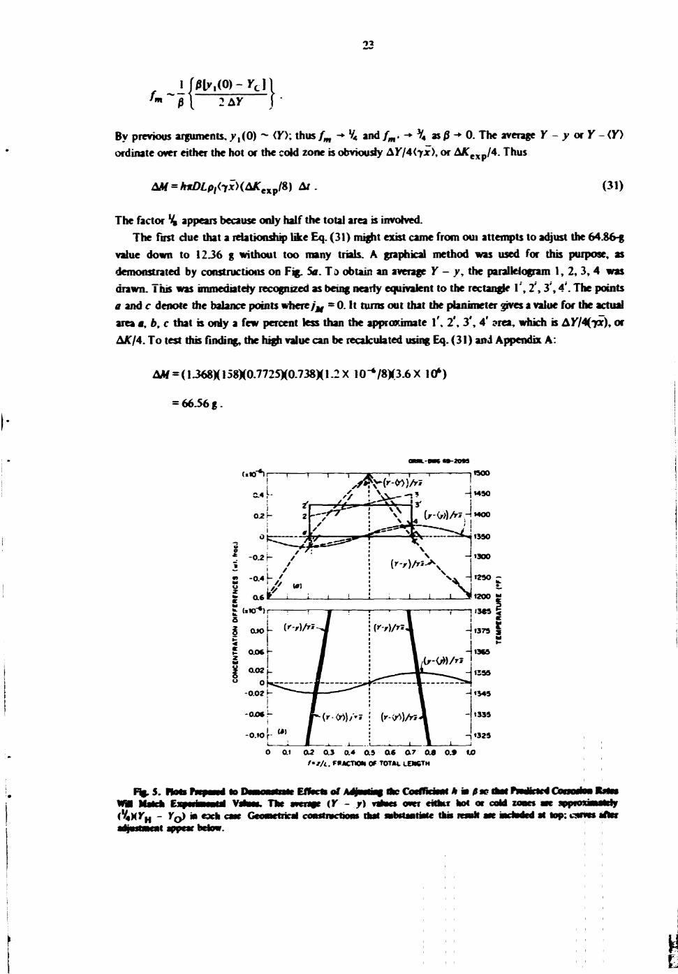
A# = AirZ>£p/<7.r>(AX:exp/8) A/ (31)

The factor % appears because only half the total area is involved. The first due that a relationship like Eq. (31) might exist came from oui attempts to adjust the 64.86-g

value down to 1236 g without too many trials. A graphical method was used for this purpose, as demonstrated by constructions on Fig. Sa. Ta obtain an average Y - y, the parallelogram 1, 2, 3 ,4 was drawn. This was immediatery recognized as being neatly equivalent to the rectangle 1', 2 \ 3', 4'. The points a and c denote the balance points where fM - 0. It turns out that the pianimeter gives a value for the actual area a, b, c that is only a few percent less than the approximate l \ 2', 3', 4' ?rea, which is AY/4(yx)t or AK/4. To test this finding, the high value can be recalculated using Eq. (31) and Appendix A:

AM = (1368X158X0.7725X0.738X1 -2X I0"*/8X3.6X 10*)

= 66.56 g.

-2099

UKf*) WOO

-|14S0

8

u 2 «•• UK) S

i <

i

-O.IO f

o o.i ou2 o.3 o.4 as as ar at M u f'f/L. FRACTION Of TOTAL LENGTH

Ffcj. S. Ptoto Piifml to Pswonlraii Effects at IJJsiiiMj Ac CtefficftMt km fitctk* VsfcM. The OTcnpe (Y - y) rmwc* over eithw hot or cold

(%HYH - Ytf m each case Geometrical comtractiom thai ssbstsatiate this lesak ace t

at top: cams after

If the average ordinate corresponding to the parallelogram had been used, the result would have been 64.34

The major implication of Eq. (31) is that &M is directly proportional to h at low values of 0. Thus an adjusted h value may be obtained by multiplying the original A by the ratio of the AATs in que?**"" That is, either

A n ew = ( p f f | ) < 4 - 2 7 X 1 0 _ 2 > s 8 1 4 X 10"3 <**!**

or

'new = (0.1906X1-368) « 0.261

The complete y curve for the new fi was plotted on Fig. 56. The/.,, is 0.241 this value in conjunction with the exact solution Tory yieldsj?, = 2.081. Thus with the ratio from Eq. (30),

2.100-2.081 ^ " 2 . 1 0 0 - 2 . 0 0 0 6 4 - 8 " 1 2 - 3 2 g -

Equation (31) would have given exactly 12.36 g.

The "Saw-Tortfc** Y(z) Fmactkm

In the previous sections, it was shown that the solution based on a tent-shaped Y{z) function could be adjusted to yield a reasonable result, if an additional mass-transfer resistance (a reaction rate constant) were invoked. It was also shown that low values of transfer all lead to an approximate form which seems to be practically insensitive to the shape of the Y(z) function - even though adjusted estimates of toiai transfer are compatible with experimental results to a limited degree. The approximate form, however, gives no definite information as to the location of deposits along z.

Suppose that the solubilities were actually lower than those adopted for this work. Then the 'is or 0*s would have to be increased to match the experimental observations (the heat transfer behavior mentioned earlier is a good example of the point under discussion), and the location of the deposits would be more clearly defined under these conditions.

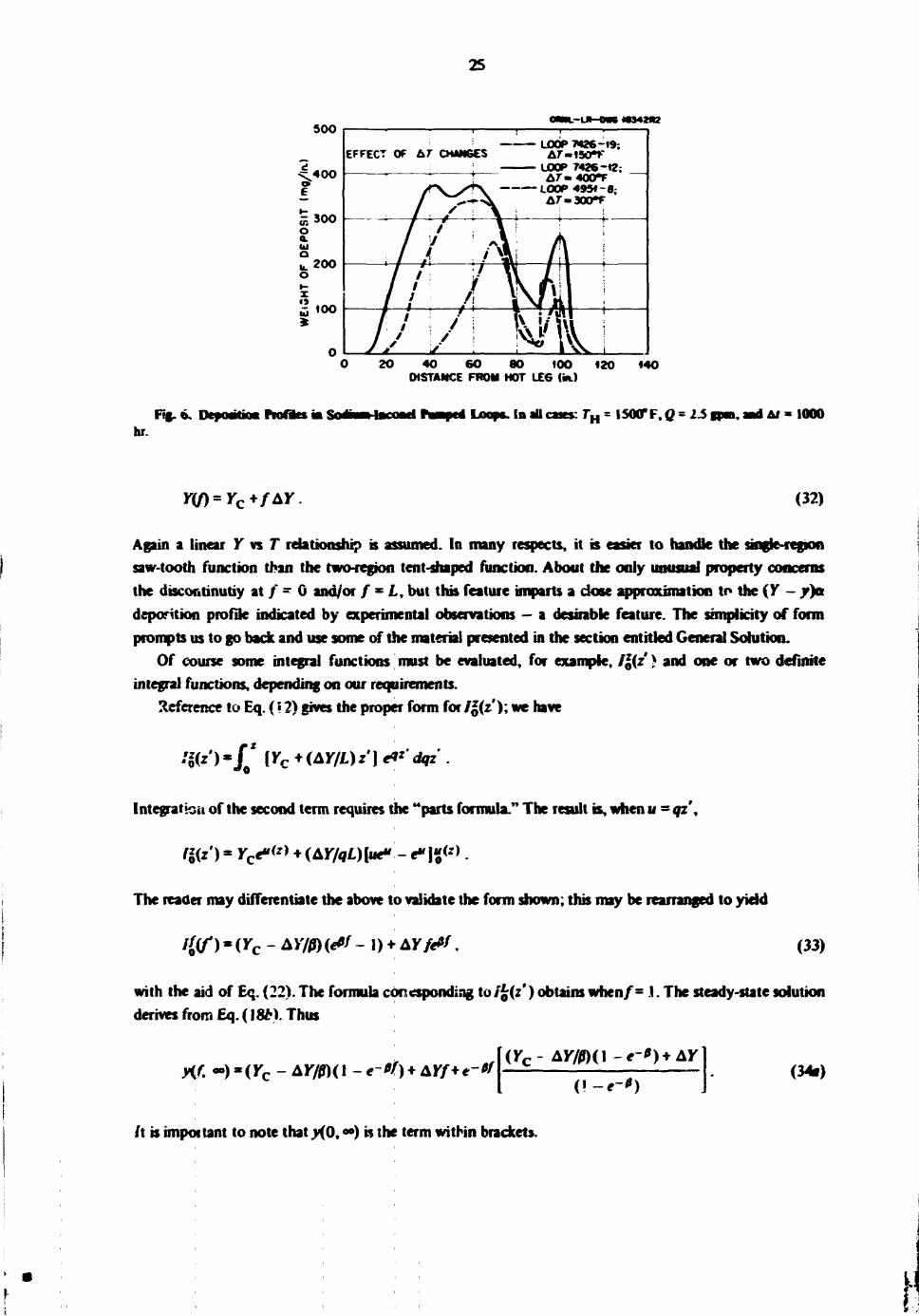
During introductory remarks, we expressed concern about the high JVR e and sudden AT in the inner tube of the heat exchanger. It now seems appropriate to present Fig. 6, which demonstrates that deposition of Ni° (ami Cr°) starts near the entrance of this tube, then exhibits a major maximum at the center or end of the tube, and finally shows a secondary maximum in the throat of the pump. Most of the deposits fall only within the short interval of / ~ 0.64 to / — 0.82 on Fig. 2. If the h and 0 values in Appendix A were indeed valid (with a k2), deposits should appear in the first and last quarters of/. Clearly they do not, and considerations of a sawtooth function seem pertinent.

The saw-tooth function given by

7U) » Tc • zi&T/L)

reflects a "driving-force" function

25

$00

4.40O

« 300 o o. u Q u. 200 o i -X o £ 100

- U H M M M M 2

EFFECT OF AT" CHANGES LOOP 7*26-19; Ar«150*F

LOOP 7426-12; AT". 400*F

LOOP 4951-8; / W - 3 0 0 T

20 40 6 0 80 100 DISTANCE FROM HOT LEG (to.)

120 140

Fig. 6. Peyortkm Profles is hr

Loops. In rfl cases TH = 150CT F, 0 = 2 3 Af'lOOO

nw-yc*/^. (32)

Agun a linear Y vs T relationship is assumed. In many respects, it is easier to handle the saw-tooth function than the two-region tent-shaped function. About the only unusual property concerns the discontinuity at / - 0 and/or / * I , but this feature imparts a dose approximation to the {Y - y)a deporition profile indicated by experimental observations — a desirable feature. The simplicity of form prompts us to go back and use some of the material presented in the section entitled General Solution.

Of course some integral functions must be evaluated, for example, /|(z' > and one or two definite integral functions, depending on our requirements.

Reference to Eq. (• 2) gives the proper form for / |(z'); we have

/ K z ' ) * / * [Yc +(AY/L)z) e**'dqz'.

lntegrattoii of the second term requires the "parts formula.** The result is, when u - qz\

f f ( z > rce*<'> + (ArMMue* -e*]«<*>.

The reader may differentiate the above to validate the form shown; this may be rearranged to yield

'Of) * <yc - A>7» («" - 1) • tX&. (33)

with the aid of Eq. (22). The formula corresponding to/£(*') obtains when/= .1. The steady-state solution derives from Eq. (18b). Thus

Hf. - ) - < r c - A K / n ( l - * - ' / ) • AK/+e-<»/ (Yc- AYMO-*"')*&

<! - *" ' ) <3*)

/t is important to note that y{0, *») is the term within brackets.

26

MoieAbotri to Approac* to Steady State

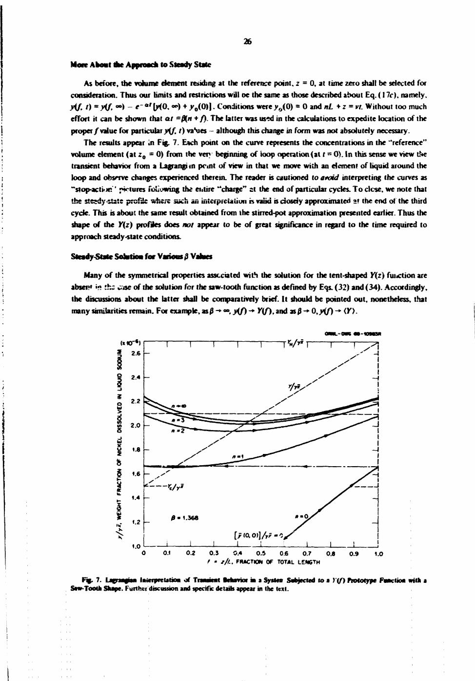
As before, the volume dement residing at the reference point, z = 0, at time zero shall be sdected for consideration. Thus our limits and restrictions will oe the same as those described about Eq. (17c), namely. y(f. t) = y{f, • • ) - * - • ' [yiO, «•) + y0iO)\. Conditions were y o ( 0 ) - 0 and nL + z = vt. Without too much effort it can be shown that at -0(n + / ) . The latter was us^d in the calculations to expedite location of the proper/value for particular yif, t) va*ues - although this change in form was not absolutely necessary.

The results appear in Fig. 7. Each point on the curve represents the concentrations in the •'reference" volume dement (at z0 - 0) from the very beginning of loop operation (at t ~ 0). In this sense we view t£»e transient behavior from a Lagrangitn point of view in that we move with an dement of liquid around the loop and obsrrve changes experienced therein. The reader is cautioned to atoid interpreting the curves as "sfop-acthjc ' pictures foiiowing the entire "charge" st the end of particular cycles. To clcse, we note that the steady =slate profile vAitrt such an inieipicUiiun is valid is ciosdy approximated at the end of the third cyde. This is about the same result obtained from the stirred-pot approximation presented earlier. Thus the shape of the Y(z) profiles does not appear to be of great significance in regard to the time required to approach steady-state conditions.

Steady-State Sofctioa for V; fiV, Many of the symmetrical properties associated with the solution for the tent-shaped Y(z) function are

absent i« :hc wise of the solution for the saw-tooth function as defined by Eqs. (32) and (34). Accordingly, the discussions about the latter shall be comparativdy brief. It should be pointed out, nonetheless, that many similarities remain. For example, as0 -»• «*, yif) -*• Yif), and as0 -*• Q,yif) -* <K>.

| 2.6

? o tal >

2.4 —

2.2

w 2.0 S - i w g 1.8 &

£ 1.6

1.4 —

1.2 -

1.0

v* ,x

rMy

1 1

H

_L J I L J_ 0.1 0.2 0.3 0.4 0.5 0.6 0.7 0.8 0.9

t - t/l., FRACTION OF TOTAL LENGTH 1.0

Ffc. 7. Layafiaw Imitipnutiom of Transient Behavior » a Systen Subjected to a )'(/) Prototype Fanction with a Saw-Tooth Shape. Further discussion and specific dctaib appear in the text.

27

Equation (34) was solved for various 0 values in order to bring forth the properties with maximum clarity. Most of the interesting features occur at z = 0 = L.so we elected to split the plots o(y(f) such that this point would appear at the center of the drawing denoted Fig. 8. We do not wish to infer through this method of presentation that a two-region solution is involved; rather we wish to stress the role of the discontinuities introduced by the Y(z) function.

The Y(0) discontinuity is of the first kind; this leads to a v(0) discontinuity of the second kind. For the time being, primary interest concerning the discontinuities on Fig. 8 is the fact that they causeyifm z x) to reside at /fO) = f(L) always. The / m a ^ cannot be found by differentiatingy(f) and setting the results equal to zero, simply because the derivative does not exist at this point. One can, however, locate fmin using the usual ptocedure outlined above.

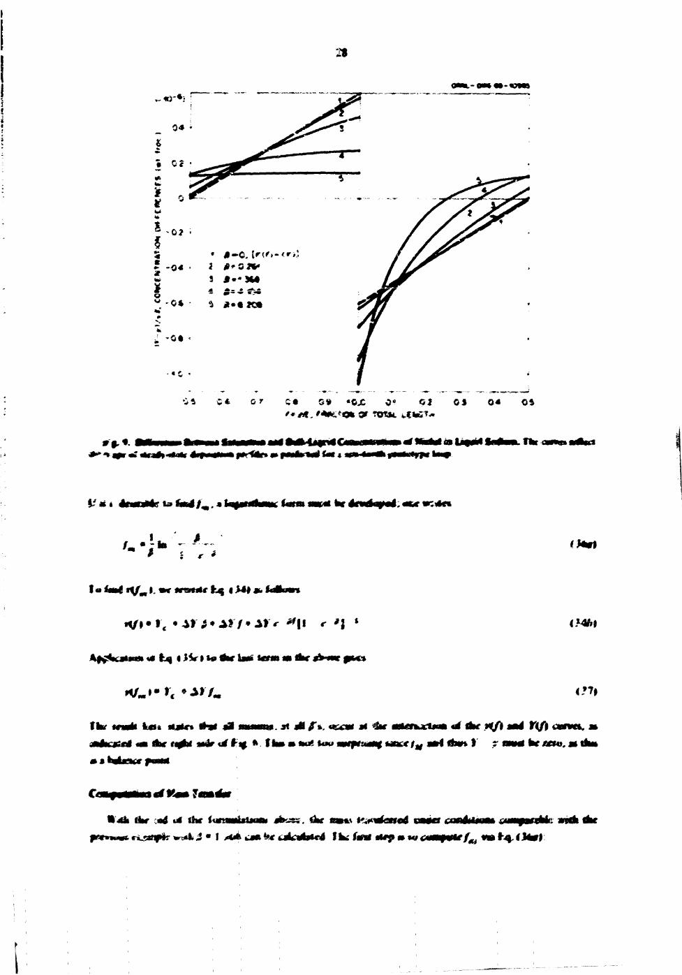
One will recall that information as to the maximum and minimum values is required in order to compute the amount ofM transferred from the hot to the cold zones. The latter is proper; iormi *° the areas under (or over) the curves presented in Fig. 9, where negative areas reflect losses by the liquid or deposition on wall surfaces and positive areas represent regions where corrosion takes place. The difference curves revert to exhibition of second-order discontinuities because Y is involved.

We now seek equations like Eqs. (28) through (30) as presented in a previous section. To obtain these, one jnly needs to fine yifm) (m represents minimum), since fm< -fmiX is known to exist at tiie origin for all r^ues of 0. The form foxy'(J) is obtained starting with Eq. (34). Thus

y'(f) = O = 0(Yc - Ar7p>-*/+ AY~(l -e-B)-*0{(\ -e~^(rc - AY/& + AY]eV. (35a)

Multiplication by 1 -e~& and performance of obvious cancellations leaves

1 -e't -0e-fifm=O. (35b)

Thus

1 -e-e=fie~fifm or e i r / ' " = p X l - e " p y i . (35c)

ORNL-OWG 69-40964

0.5 0.6 0.7 0.8 0.9 4 .0 ,0 0.1 0.2 0.3 0.4 0.5

f'l/L . FRACTION OF TOTAL LENGTH

Fig. 8. Predicted Baft-Liquid Concentrations of Nickel in Sodium for a "Saw-Tooth" Prototype Lo*p. Carves apply at steady-state operation; they demonstrate the effect of varying 0.

2t

.- «-•:•

*

M

, 0 « <

«c

S 1 - * 3 M

0 * • * * • • * £ *

i 4 C t o r C« 0 * »0X 0? O l OS 0« 0 4

I?. u,fmiim.» tmm V « M f l

* * • * *

!« 4w< »V* I- •* *rot*f hq I >«# *

•</»•»< •^r^*^i7*^rr ^|i r *j * iMftl

A f f « K * * a » *• fcq I J * r i t « * r lw§ tend « i

1A«»* *« * - * * / . <H»

I k . «tfi to ft^tf Mdr uf f ^ * f fa* m «uS tow

«f *SUr *d+* #f* mi Yifi wHftrwmj *mL*tM ami i&m% f bc/£S43.Mihm

• »

T i

•'<& the cad uf the ifctss. 4w saw %f^.ydontA

29

From Eq. i 37j> »« fmd

>ifm • f c 11 -5 • u .:xo.444>| x io"* * :.o>;= x io"* .

To find .tt Of we merel>' compute the fame from its formula:

yiQl-y{fm.\* Yc - \Ylfi+ &Yi\ -e-*y%

'%*.$ - 0.*77) • ( I J/0.74561) X 10 "*

« 2 J33 X 10"* .

Vo». in fcq. I »Of. 2{<Y> , K / « M ' T * * eojwvakni to \y{Q) - yifm\\\yx in the present case The value is 'OX 10 '" m each case: so the answer wiH come out exactly the same as found previously. 64.86 g.

Of course this « mudi too hajt and another approximate form is sought. The approach is the same as before: we seek the limit o f / m as 0 -* «•. We have

P

where* *< I - e-*M.AppHcak cs of LHofpitafsnrfe once leaves

which constitutes a new problem to which the nde may be reapplied. Thus

/. *-Hfi+H-e-*„ L 0 * ' - I

One mote application yields

L fm* L *—. t~m e**e* • 1 2

*ow we know that/„ * 0 . 5 0 . / l - . « 0 «/.. and*/ ) *<]T> at Icw0. This takes us right back to Eq.(3l) for an approximate form. Obviously the numerical results witt ako he identical. Thus we join in Epsteins conrluuon.4 that the approximate form fat JJtft from any reasonably shaped Y(z) function is the same. However, the shape of Wzj does have a marked influence on the location of the predicted deposition profile, even at low fi valines, as imifratrd in Fig. 9.

30

DISCUSSION

Concerning the Geaerol Solution

The mathematical solution of the problem posed by Eqs. (3)-(S) proceeded in three steps, first, the independent variables were traraformet to the pseudo-Lagrangian variables (z , 7), in terms of which Eq. (3) became an ordinary differential equation in z, with 7 appearing only as a parameter. Second, this equation was integrated, thereby introducing as the constant of integration an arbiter/ (at this stage) function ${t). Finally, the inverse transformation to independent variables yz, i) was performed, and various algebraic manipulations were executed *c and 0(7) in terms of the assumed given inital concentration y0(z). The mathematical expression of the loop closure, Eq. (5), played a crucial role in the manipulations in this final stage.

At this point it should be mentioned that the transient treatment of Keyes14 seems to be incorrect, because he apparently makes the unjustified assumption thai the function #(/) is lincai. This error does noi have z great significance, since most *i Keyes' vork is concerned with the steady state, which is treated ca.-rectly.

It would have been just as easy, perhaps easier, to solve th? problem with the initial condition (4) replaced by a condition of the form

A0,t) = Mt), 0<t</./v, (4)

with iiyt) known. The condition (4) corresponds to a starting procedure in which the loop is filled at the reference point, z ~ 0, from a reservoir containing fluid with a known concentration of solute. By way of contrast, the condition actually used, Eq. (4), corresponds to a procedure in which the loop is already filled at time zero. Furthermore, the solute concentration is known throughout the loop at this time. Thus (4) seems more appropriate than (4), in view of the actual starting procedure as discussed in the section Transient Behavior.

In obtaining Eq. (17a) it was assumed that z0 - 0. The corresponding equation for arbitrary z0 is

^/)«r"y,(z 0) + r^ I —p-(n — \)qL

(38)

where, as before, z 0 = nL + z - vt, with n the number of cycles having been undergone by the particle at z at time /. In order to obtain a "stop-action" picture of the solute distribution .y as a function of z for fixed /, one simply establishes the desired value of/ and then computes the right-hand side for various values of z, noting that z 0 is a function of z. In most of the presentations of this report, the contrary option of fixing z 0 *«as selected. With the particular choice z 0 = 0, the computations were considerably simplified, and the resulting Lagrangian (particle following) gives at least as good a physical picture of the solute distribution in the stream as would a plot of y vs z for fixed t.

Finally, it should be mentioned that we have solved Eq. (3) by Laplace transform techniques. However, this only provided an alternate way of obtaining Eq. (11), and the really difficult part, evaluation of the constant of integration #7 - z/v) in terms of the given initial distribution y0, still has to be performed laboriously, as shove.

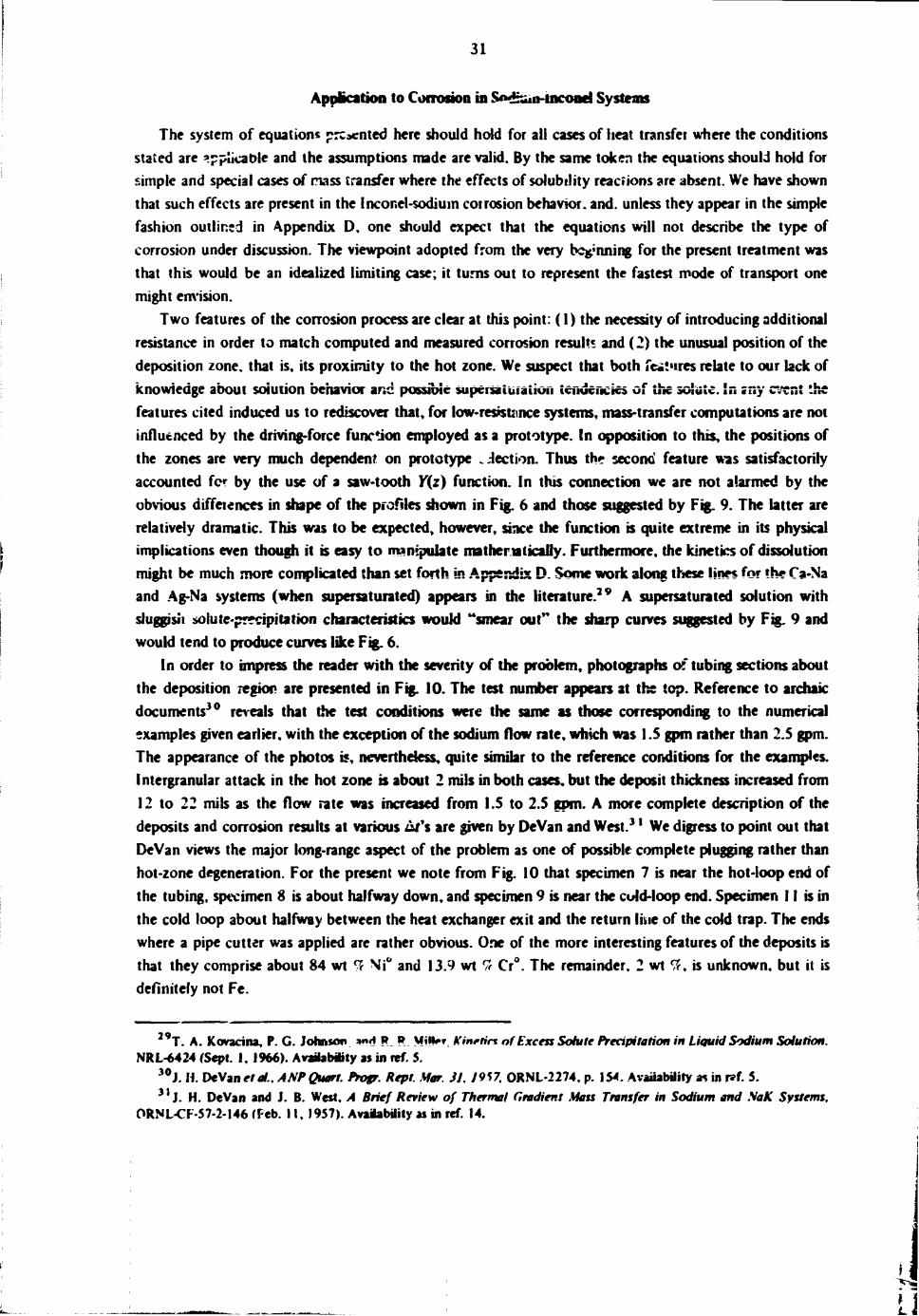
31

Application to Corrosion in S*£uin-Mcoiiei Systems

The system of equations presented here should hold for all cases of heat transfer where the conditions stated are applicable and the assumptions made are valid. By the same token the equations should hold for simple and special cases of mass transfer where the effects of solubility reactions are absent. We have shown that such effects are present in the Inconel-sodium cotrosion behavior, and. unless they appear in the simple fashion outlined in Appendix D, one should expect that the equations will not describe the type of corrosion under discussion. The viewpoint adopted from the very beginning for the present treatment was that this would be an idealized limiting case; it turns out to represent the fastest mode of transport one might envision.

Two features of the corrosion process are clear at this point: (1) the necessity of introducing additional resistance in order to match computed and measured corrosion result* and (2) the unusual position of the deposition zone, that is, its proximity to the hot zone. We suspect that both features relate to our lack of knowledge about solution behavior and possible supcraiufaiion tendencies of the solute. In «ny event the features cited induced us to rediscover that, for low-resistance systems, mass-transfer computations are not influenced by the driving-force function employed as a prototype, tn opposition to this, the positions of the zones are very much dependent on prototype . .-lection. Thus the second feature was satisfactorily accounted for by the use of a saw-tooth Y(z) function. In this connection we are not alarmed by the obvious diffeiences in shape of the profiles shown in Fig. 6 and those suggested by Fig. 9. The latter are relatively dramatic. This was to be expected, however, since the function is quite extreme in its physical implications even though it is easy to manipulate mathenaticaliy. Furthermore, the kinetics of dissolution might be much more complicated than set forth in Appendix D. Some work along these lines for the Ca-Na and Ag-Na systems (when supersaturated) appears in the literature.29 A supersaturated solution with sluggish 5olute-pr*cipitation characteristics would "smear out" the sharp curves suggested by Fig. 9 and would tend to produce curves like Fig. 6.

In order to impress the reader with the severity of the problem, photographs of tubing sections about the deposition region are presented in Fig. 10. The test number appears at the top. Reference to archaic documents30 reveals that the test conditions were the same as those corresponding to the numerical examples given earlier, with the exception of the sodium flow rate, which was 1.5 gpm rather than 2.5 gpm. The appearance of the photos is, nevertheless, quite similar to the reference conditions for the examples. Intergranular attack in the hot zone is about 2 mils in both cases, but the deposit thickness increased from 12 to 22 mils as the flow rate was increased from l.S to 2.5 gpm. A more complete description of the deposits and corrosion results at various £/'s are given by DeVan and West.3' We digress to point out that DeVan views the major long-range aspect of the problem as one of possible complete plugging rather than hot-zone degeneration. For the present we note from Fig. 10 that specimen 7 is near the hot-loop end of the tubing, specimen 8 is about halfway down, and specimen 9 is near the cold-loop end. Specimen 11 is in the cold loop about halfway between the heat exchanger exit and the return line of the cold trap. The ends where a pipe cutter was applied are rather obvious. One of the more interesting features of the deposits is that they comprise about 84 wt <% Ni° and 13.9 wt £ Cr°. The remainder. 2 wt # , is unknown, but it is definitely not Fe.

2 9 T . A. Kovacina, P. G. Johnson »»»d P.. * M!**r Kineticx of Excess Solute Precipitation in Liquid Sodium Solution. NRL-6424 (Sept. 1. 1966). Availability as in ref. 5.

3 0 J . H. DeVan etd.. ASP Quart. Prop. Rept. Mar. SI, 19SJ, ORNL-2274, p. 154. Availability as in r»f. 5. 3 ' J. H. DeVan and J. B. West. A Brief Review of Thertrvl Gradient Mass Transfer in Sodium and SaK Systems.

ORNL-CF-57-2-146 (Feb. II, 1957). Availability as in ref. 14.

i \

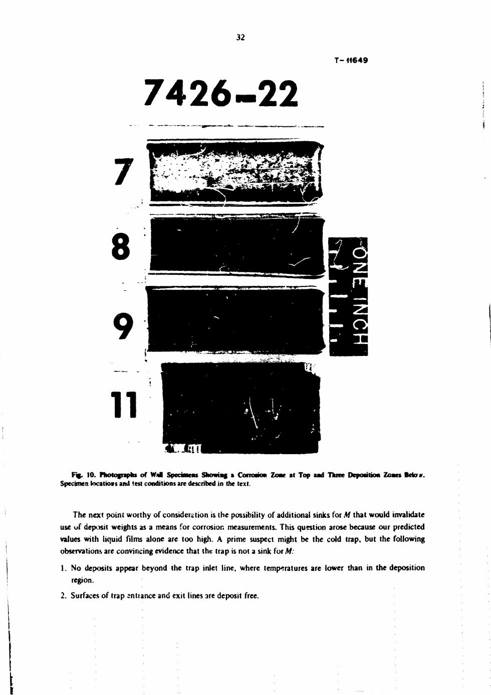
32

T- 41649

7426-22

7

8

9

11 Fig. 10. Photographs of Wal Specimen* Showing a Corrosion Zone at Top and Three Deposition Zones Below.

Specimen locatioB* and lest conditions are described in the text.

The next point worthy of consideration is the possibility of additional sinks for M that would invalidate use of deposit weights as a means for corrosion measurements. This question arose because our predicted values with liquid films alone are too high. A prime suspect might be the cold trap, but the following observations are convincing evidence that the trap is not a sink for M:

1. No deposits appear beyond the trap inlet line, where temperatures are lower than in the deposition region.

2. Surfaces of trap enhance and exit lines are deposit free.

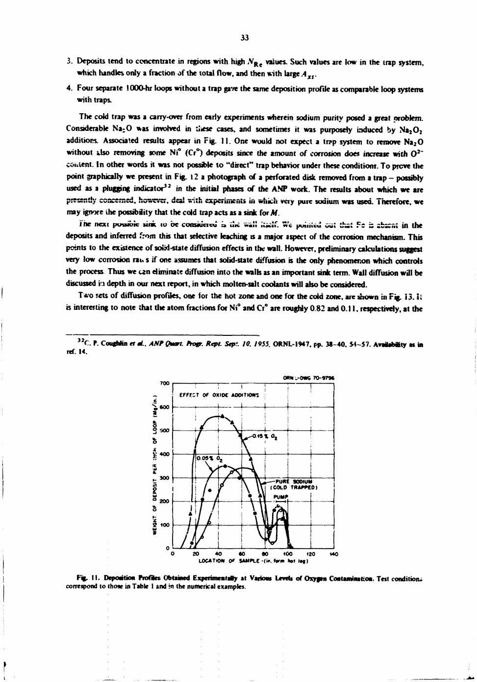
33

3. Deposits tend to concentrate in regions with high ,V R e values. Such values are low in the trap system, which handles only a fraction of the total flow, and then with large Axs.

4. Four separate 1000-hr loops without a trap gave the same deposition profile as comparable loop systems with traps.

The cold trap was a carry-over from early experiments wherein sodium purity posed a great problem. Considerable Na : 0 was involved in tiiese cases, and sometimes it was purposely induced by Na 2 0 2

additions. Associated results appear in Fig. 11. One would not expect a tr?p system to remove Na 2 0 without viso removing some Ni° (Cr°) deposits since the amount of corrosion does increase with O2" content. In other words it was not possible to "direct" trap behavior under these condition!. To prove the point graphically we present in Fig. 12 a photograph of a perforated disk removed from a trap - possibly used as a plugging indicator32 in the initial phases of the AMP work. The results about which we are pi scrttiy concerned, however, deal with experiments in which very pure sodium was used. Therefore, we may ignore ihe possibflity that the cold trap acts as a sink for A/

The ncxi pvoibic sink io be conswcicu a liti »«!! Half. «i'e puimcU out thit Fc i zb2Z7*l in the deposits and inferred from this that selective leaching is a major aspect of the corrosion mechanism. This points to the existence of solid-state diffusion effects in the wall. However, preliminary calculations suggest very low corrosion rau s if one assumes that solid-state diffusion is the only phenomenon which controls the process Thus we tan eliminate diffusion into the walk as an important sink term. Wall diffusion will be discussed i.i depth in our next report, in which molten-salt coolants will also be considered.

Two rets of diffusion profiles, one for the hot zone and one for the cold zone, are shown in Fig. i3. i; is interesting to note that the atom fractions for Ni° and Cr° are roughly 0.82 and 0.11, respectively, at the

3 2 , X. P. CoujHhn et tL, AN? Quart, frop. Rept- Sep:. 10, 1955. ORNL-1947, pp. 38-40. 54-57. AvaMabaity as in ref. 14.

700 0*H _-DWG 70-9796

20 40 60 80 100 120 LOCATION 0 * SAMPLE -(ii». form hot Itg)

140

Fig. 11. Deposition Profles Obtained Experiments*? at Various Levels of Oxynen Contamimtion. Test condition-correspond to those in Table I and in the numerical examples.

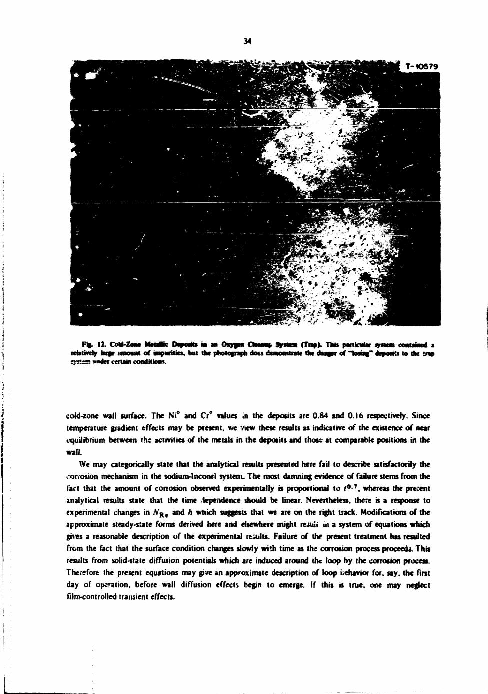
34

F*. 12. CoU-Zoaw lliiilir Dojoaiii m am Oxygm C h i t S»rt— (Top). Tte particular systtn rnnniwtJ a icbtmly bite MMMUM of iaapwitiei. but the photograph docs denoastrate the daager of "to a t " depoass to the trap gyg^a under certain condHioas.

cold-zone wall surface. The Ni° and Cr° values in the deposits are 0.84 and 0.16 respectively. Since temperature gradient effects may be present, we view these results as indicative of the existence of near equilibrium between the activities of the metals in the deposits and those at comparable positions in the wall.

We may categorically state that the analytical results presented here fail to describe satisfactorily the corrosion mechanism in the sodium-! nconcl system. The most damning evidence of failure stems from the fact that the amount of corrosion observed experimentally is proportional to f ° - 7 , whereas the present analytical results state that the time dependence should be linear. Nevertheless, there is a response to experimental changes in JV R e and h which suggests that we are on the right track. Modifications of the approximate steady-suite forms derived here and elsewhere might rejuli iii a system of equations which grves a reasonable description of the experimental results. Faflure of the present treatment has resulted from the fact that the surface condition changes slowly with time as the corrosion process proceeds. This results from solid-state diffusion potentials which are induced around the loop by the corrosion process. Therefore the present equations may give an approximate description of loop behavior for. say, the first day of operation, before wall diffusion effects begin to emerge. If this is true, one may neglect film-controlled transient effects.

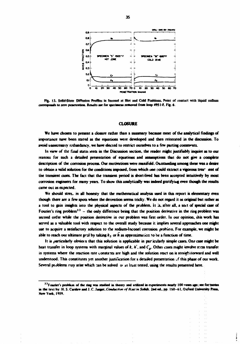
3S

H _ * : k r 5 ash snamn "V « » # r - i- VCONCM **r «w» -j _, a4»-

WT XOK COLO X*K ~t

- r-

OJ k "T ir r#

2O3O40SOW7O0 e n s> « K n n ETIUtIO*

fro* loop 4951-8. F t *.

CLOSURE

We have chosen to present a closure rather than a summary because roost of the analytical findings of importance have been stated as the equations were developed and then reiterated in the discussion. To avoid unnecessary redundancy, we have elected to restrict ourselves to a few parting comments.

In view of the final statements in the Discussion section, the reader might justifiably inquire as to our reasons for such a detailed presentation of equations and assumptions that do not give a complete description of the corrosion process. Our motivations were manifold. Outstanding among these was a desire to obtain a valid solution for the conditions imposed, from which one could extract a vigorous rxea* «nt of the transient cases. The fact that the transient period is short-lived has been accepted intuitively by most corrosion engineers for many years. To show this analytically was indeed grafifyMg even though the results came out as expected.

We should sires* hi all honesty that the mathematical analysis used in this report is elementary even though there are a few spots where the derivation seems tricky. We do not regard it as original but rather as a tool to p i n insights into the physical aspects of the problem, it '<&. after all, a sort of special case of Fourier's ring problem3 ' - the only difference being that the petition derivative in the ring problem was second order while the position derivative in cur problem was first order. In our opinion, this work has served as a valuable tool with respect to the overall study because it implies several approaches one might use to acquire a satisfactory solution to the sodhmvlnconei corrosion profeiem. For example, we aught be able to reach our ultimate gral by taking * 2 or * as approximation to be a function of time.

It is (particularly obrkx-s that this solution is applicable in par icubriy simple cases. One case might be heat transfer in loop systems with marginal values of* . h\ and Cp. Other cases might involve nvas transfer in systems where the reaction rate constants are high and the solution read on is strakjhiiocward and well understood. This constitutes yet another justification for a detailed presentation J, this phase of our work. Several problems may arise which -an be solved or at bust tested, using the results presented here.

, )FoMkr'« problem of die ring was studied in theory and utilized in experiments nearly 100 vests ago; see foe notes in tke text by: H. S. Cantow sad J. C. Janjrr. Comhtciitm ofHcii in Sobds, 2nd etf.. pp. 140-61. Oxford Unwemty Pre* New York. 1959.

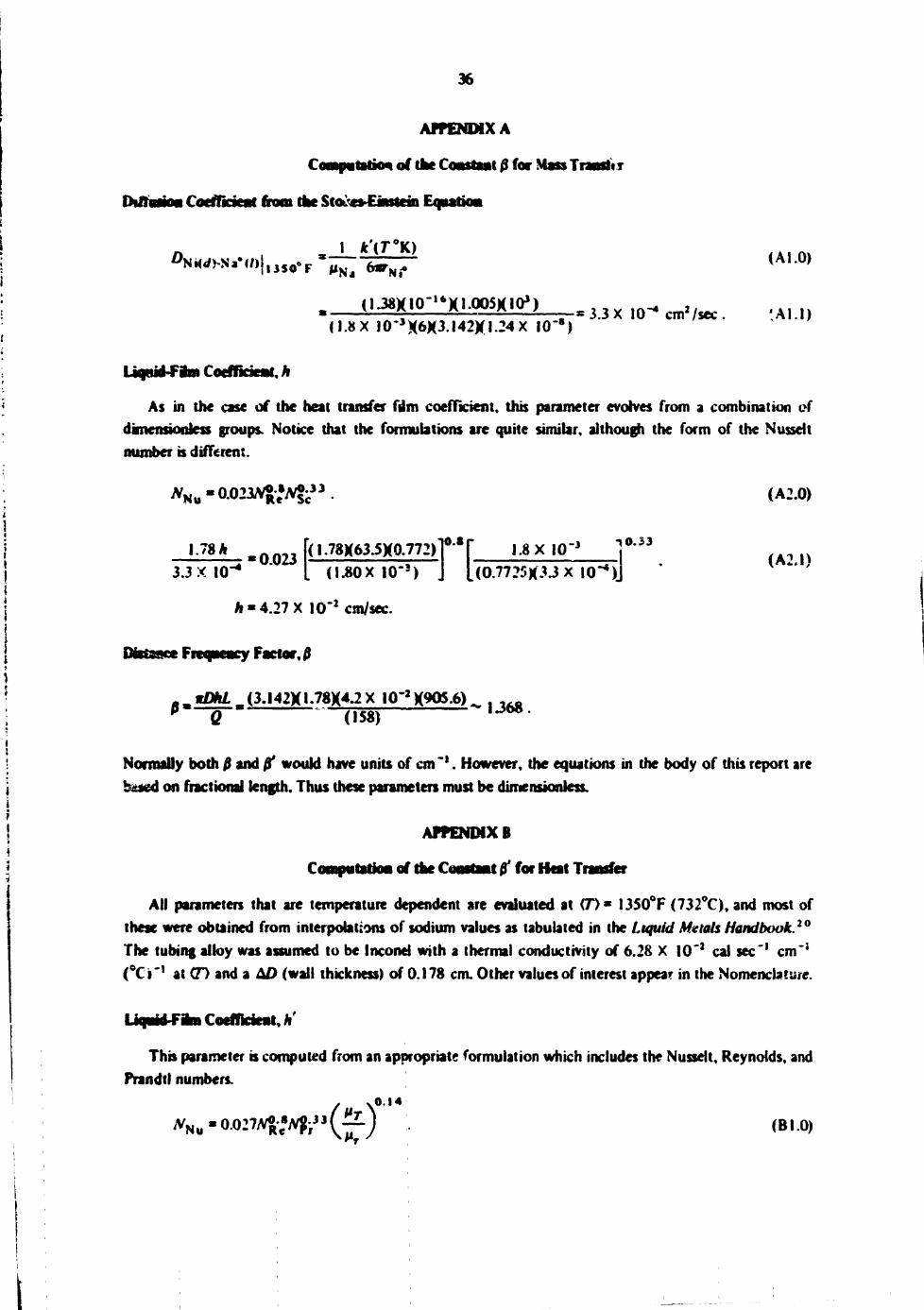
36

APfENDIXA

CoaapatatMm of the Constant 0 for

Di/ruMM Coetfkienf from the Sto&s-Enstein Equation

».T

- • i » » ! i *'(r°K)

O^xio'^xioosxio3) (1.8X 10-SK6X3.I42)(I.24X lO'*)

= 3.3X 10"4 cm2/sec

(A1.0)

tAl.I)

As in the case ct the heat transfer film coefficient, this parameter evolves from a combination of dimensionless groups. Notice that the formubtions are quite similar, although the form of the Nusseit number is different.

^u«0 .023A*»A& .33

1.78 A 3.3 X 10

- « 0.023 (1.78K63.5X0.772)]0'8[" 1.8 X 1 0 ' 3 ] ° " 3 3

. (I.80X 1 0 ° ) J 1(0-7725X33 X I0"*)J

(A2.0)

(A2.I)

A-4.27 X 10~2 cm/sec.

Dfetaace Freoneacy Factor, 0

fl,«0m-(3.l42X».78X4.2X lQ-*X90S-6)^ ^ p e (i58) • • x w *

Normally both 0 and 0* would have units of cm"1. However, the equations in the body of this report are beted on fractional length. Thus these parameters must be dimensionless.

APPENDIX B

Computation of the Constant 0' for Heat Transfer

All parameters that are temperature dependent are evaluated at CD* 1350°F (732°C), and most of these were obtained from interpolations of sodium values as tabulated in the Liquid Metals Handbook.20

The tubing alloy was assumed to be Incond with a thermal conductivity of 6.28 X 10~2 cal sec'1 cm"1

(°Ci~! at <D and a 6D (wall thickness) of 0.178 cm. Other values of interest appear in the Nomenclature.

Uqatd-Fim Coefficient, h'

This parameter is computed from an appropriate formulation which includes the Nusseit, Reynolds, and Prandt! numbers.

.0.14

(BIO) *Nu-°027Afc»ivfc»(^)

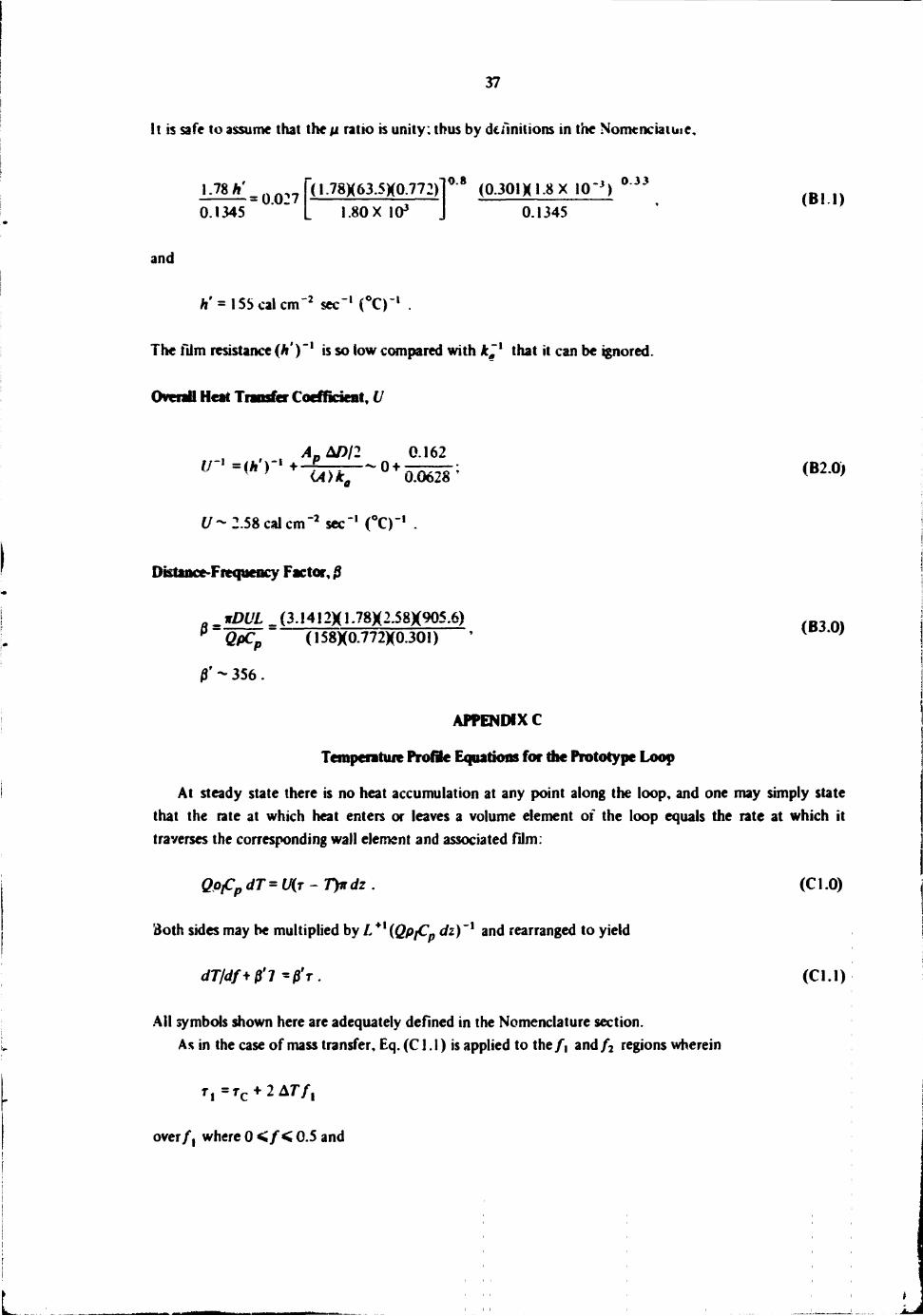
37

It is safe to assume that the ji ratio is unity; thus by definitions in the Nomenciaiuie.

i ^ = 0.027 N 0.1345 L

(1.78X63.5X0.772) 1.80 X 103

0 8 (0.301X1-8X I P ' 3 ) ° 3 3

0.1345 (B l l )

and

V = l55calcm- 2 sec - ' (°C)

The film resistance (h ) is so low compared with k~l that it can be ignored

Overall Heat Transfer Coefficient, U

IT 1 = i /»V' +•-* C4>*„

0.162 0.ut>ze (B2.0)

( / -2 .58ca l cm - 2 sec" 1 (°C) -2 ,^,-1 /°r\-l

Distance-Frequency Factor, 0

*DUL (3.1412X1.78X2.58X905.6) QfiCB~ (158X0.772X0.3OI)

0' - 356

(B3.0)

APPENDIX C

Temperature Profile Equations for die Prototype Loop

At steady state there is no heat accumulation at any point along the loop, and one may simply state that the rate at which heat enters or leaves a volume element of the loop equals the rate at which it traverses the corresponding wall element and associated film:

Qpfi dT=U{r- TJndz (C1.0)

- \ - i Both sides may be multiplied by L (Qp/Cp dz) and rearranged to yield

dT/df+0'7 *P'T (Cl.l)

Ail symbols shown here are adequately defined in the Nomenclature section. As in the case of mass transfer, Eq. (C1.1) is applied to the fx and f2 regions wherein

T I = T C + 2 A 7 ' / 1

over/, where 0 < / < 0.5 and

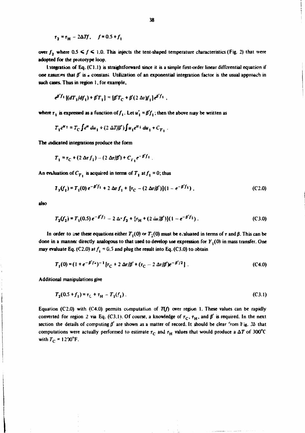
38

T 2 = T H - 2 A 7 7 . / « 0 . 5 + / ,

over f2 where 0.5 < / < 1.0. This injects the tent-shaped temperature characteristics (Fig. 2) thai were adopted for the prototype loop.

Integration of Eq. (CI .1) is straightforward since it is a simple first-order linear differential equation if one tssun:-*s that & is « constant Utilization of an exponential integration factor is the usual approach in such cases. Thus in region 1, for example,

e*'« 1<</7V<*/,) + ^ r , J - [0Y C + ^(2 AT)/-,]**'« ,

where r, is expressed as a function of/,. Let u\ = 0'/,; then the above may be written as

Tx*1 - r c j c " c / « l T ^ a / / p i j a 1 e - ' a i i 1 + c 7 . j

The indicated integrations produce the form

r l - T c + ( 2 A r / 1 ) - ( 2 A r / t f ) * C J . | e - * V

An evaluation of CT is acquired in terms of Tx at/, = 0; thus

M W - r ^ e - ' t t + 2 AT/ , + [ T c _ ( 2 Ar/0')](1 - e "*''»), (C2.0)

also

W ) s r»(°- 5) «~* / a - 2 A-/ 2 + [fH + (2 <•,#)](1 - e-*''*) . (C3.0)

In order to use these equations either T,(0) or 7*2(0) must be equated in terms of r and 0. This can be done in a manner directly analogous to that used to develop uie expression for Yx(0) in mass transfer. One may evaluate Eq. (C2.0) at / , - 0.5 and plug the result into Eq. (C3.0) to obtain

T,(0) =(1 + e-*r*Y! [TC + 2 Ar/0' + (r c - 2 Ar/0>-''/*] . (C4.0)

Additional manipulations give

r2(o.s + / , ) « T C + TH - r,^,). (C3.i)

Equation (C2.0) with (C4.0) permits computation of 1\f) over region 1. These values can be rapidly converted for region 2 via Eq. (C3.1). Of course, a knowledge of r c , r H , and 0' is required. In the next section the details of computing $ are shown as a matter of record. It should be clear crom Fig. Zb that computations were actually performed to estimate r c and rH values that would produce a AT of 300°C with Tc = 1200°F.

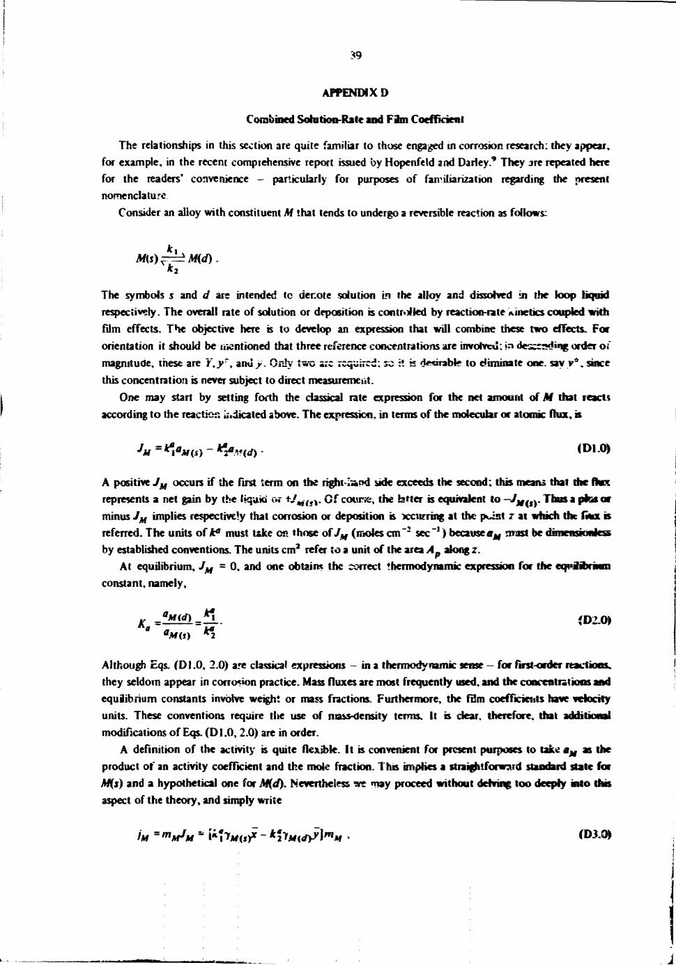
<9

APPENDIX D

Combined Solution-Rate and Fifan Coefficient

The relationships in this section are quite familiar to those engaged in corrosion research: they appear, for example, in the recent comprehensive report issued by Hopenfeld and Darley.9 They are repeated here for the readers' convenience - particularly for purposes of familiarization regarding the present nomenclature

Consider an alloy with constituent M that tends to undergo a reversible reaction as follows:

Ai*(s)f-=^Af(</).

The symbols s and d are intended tc denote solution in the alloy and dissolved in the loop liquid respectively. The overall rate of solution or deposition is controlled by reaction-rate kinetics coupled with film effects. The objective here is to develop an expression that will combine these two effects. For orientation it should be mentioned that three reference concentrations are involved: >n descending order of magnitude, these are Y,y^, anu>. Only two arc required: so :• is durable to eliminate one. say v*. since this concentration is never subject to direct measurement.

One may start by setting forth the classical rate expression for the net amount of M that reacts according to the reaction indicated above. The expression, in terms of the molecular or atomic flux, is

•^ - * i « j f ( s ) - * !« .vcd ) - < D , 0 >

A positive JM occurs if the first term on the right hand side exceeds the second; this means that the flux represents a net gain by the liquid or * /„ /o- Of course, the fetter is equivalent to —•J^,sy Thus a pfcs or minus JM implies respectively that corrosion or deposition is xcuning at the point z at which the fiux is referred. The units of A4 must take on those ofJM (moles cm ~2 sec - 1 ) because ffj, most be dirnenskjniess by established conventions. The units cm3 refer to a unit of the area Ap along z.

At equilibrium, JM = 0, and one obtains the correct thermodynamic expression for the earaHbraan constant, namely,

K -=**<*) =** (D2-0)

Although Eqs. (Dl.0, 2.0) are classical expressions - in a thermodynamic sense — for first-order reactions. they seldom appear in corrosion practice. Mass fluxes are most frequently used, and the concentrations and equilibrium constants involve weight or mass fractions. Furthermore, the film coefficients have velocity units. These conventions require the use of mass-density terms. It is dear, therefore, that additional modifications of Eqs. (D1.0,2.0) are in order.

A definition of the activity is quite flexible. It is convenient for present purposes to take aM as the product of an activity coefficient and the mole fraction. This implies a straightforward standard state for M(s) and a hypothetical one for M(d). Nevertheless we niay proceed without delving too deeply into this aspect of the theory, and simply write

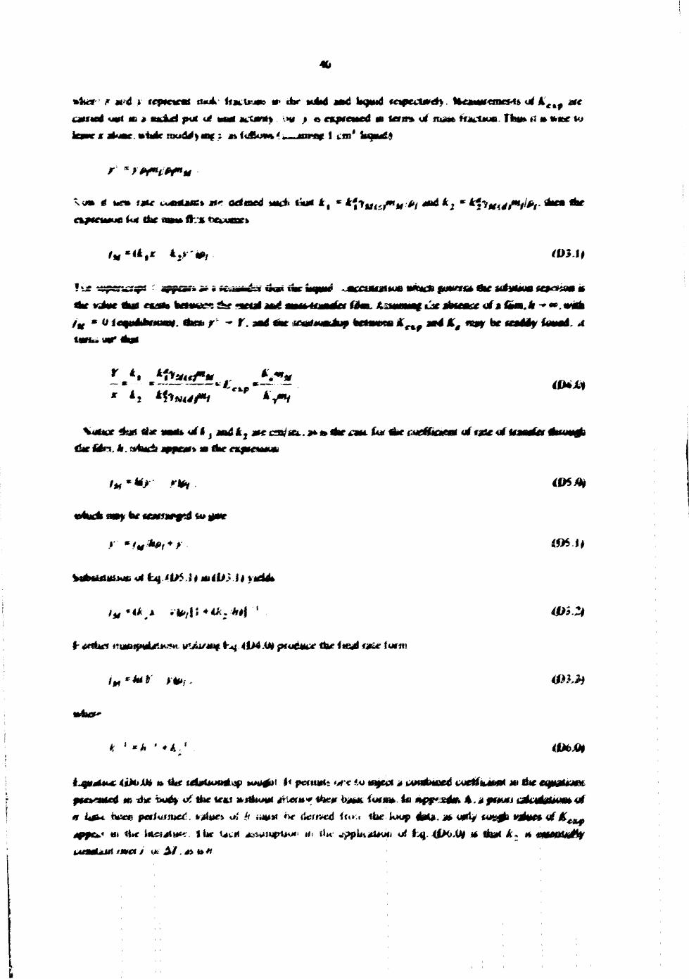
m

•fear- F «t<4 i t c y c g i tt*A <{icbua» *> tftw «uM aad l*)M*d fcape<ai*4t. HrfanwrrwMfc utf A c t y aft earned ««»t m » sit&d put ** M * a i t * * } HI j © Arretted at %aw% id tu*m> Hat-feus. Tfttf* rt » «•** to

r sf<y«</#f««

.«Mfc * W « f * t * U4MUMEI JfT OdattA Mick tali* 4 , s *'?jtf*.'y M * / * * * *J * *2?*4# ,/*#^'/-

/ * « a , r 42*-««, /1>5 J#

l i s A .- -4

r'' -* T. a«d «ar« l c*# m4 tit f*»y far ceadty imtmd A

— m - - w ™ *L ***** *M>

v*f <P*X*

€M §Hm. h. avfa«& appear* *» A<r O ^ M M M I

/ * * * > *¥y flfci9»

«dycfc a»y W «s*farf*d ftu aw*

«>M>

MbiUtttiMti 44 fc^JU5 it miUZU *****

' * * < * « * • *v is • < * • • * * ! ' 0**3

4- «rcb<9 t?utf»*fNtf>.*u«*L tf*&/*tt£ t ^ 4lM.U» puidavf tfcr fieai «»£* fur«)

/ * * * * * >*», <#?,#

* ' « A • *k.% OM>m

ijyt***- iiktih » 4*t tAj/Uon+isp MHt^it 4< |HM«n*tt w< *o marcf * amdmmi cut&uMtiA m lite tqp&nm p*€wu4 m the i*ad> */, fbe %t*s »«fWtf4 aH*ri»* <*»«•- b*m i<*jt* is aifpiusd* A.ii jmofj r^rilfafrift ^