Unsupervised Learning and Dimensionality Reduction A Continued Study on Letter Recognition and Adult Income

Dudon Wai, dwai3

Georgia Institute of Technology CS 7641: Machine Learning

Abstract: This paper explores various algorithms for clustering and dimensionality reduction as pre-processing techniques prior to implementing supervised learners to the dataset.

Introduction

This project builds on the concepts of supervised learning from Assignments 1 & 2 by exploring different clustering and dimensionality reduction algorithms. The purpose of the assignment is to use clustering and dimensionality reduction to pre-process the data to train decision trees and neural networks. Two clustering algorithms were explored: k-means and expectation maximization (EM). Four dimensionality reduction methods were implemented: principal component analysis (PCA), independent component analysis (ICA), random projection (RP) and information gain (as the method of choice). The paper is structured in 3 main sections: Part 1 applies clustering to two datasets, Part 2&3 applies dimensionality and re-clustering to two datasets and Part 4&5 applies dimensionality and re-clustering with neural networks.

Datasets

Both datasets used were explored in Assignment 1 and were originally taken from the UCI machine learning repository. The Letter Recognition dataset (LEFT) is a classification dataset and the Adult Income dataset (RIGHT) is a classification dataset. The attributes are displayed here, and the output class is the last square.

Dataset 1: Letter Recognition

Computer vision is a fast-growing field within machine learning as algorithms, hardware and cloud computing are finally coming together to make technologies viable, such as virtual reality, augmented reality and autonomous vehicles. Within the field of computer vision, optical character recognition (OCR) plays an important role in the advance of technology. Many industries such as healthcare, finance, law and construction have used OCR to help with paperwork reduction, process improvement and task automation. A study of the accuracy of OCR is important to the computer vision industry, as it is more mature and can be used as a guide when developing for more difficult sub-domains like video tracking and object recognition.

The letter recognition dataset contains 26 classes (one for each letter in the alphabet), 16 attributes (position, length, statistical moments), and 20,000 instances of user-generated letters based on a variety of fonts. Dataset 1 is interesting with respect to machine learning because the numeric features and equally occurring classes make Letter Recognition a good candidate for using clustering and dimensionality to train a neural network.

Dataset 2: Adult Income

In the last decade, the global population living in poverty (defined as living with less than $2 per day, 1985 prices) has decreased dramatically from 80% in 1920, to 50% in 1970 to 10% in 2015 [1]. Similarly, the standard of living in nations globally is on the rise [2]. National policy plays a role in achieving this prosperity. In order for governments to determine changes in policy, it uses data to measure previous and current states. A primary resource for governments is census data, which collects socio-economic details of the population. Dataset 1 is a subset from the 1994 US Census, which is used to relate education, heritage and age (among others) against income, in this case, whether income is above or below $50,000 per year. Governments can use this data to determine the most impactful factors for increasing household income.

The dataset consists of 2 classes (<=$50k, >$50k), 14 socio-economic attributes, and over 30,000 instances which allows for sufficiently large subsets when splitting the overall dataset into training, validation and test sets. In terms of machine learning, Dataset 2 is interesting because of the challenge of training a learner based on an unevenly distributed output class (24,720/7,841) as observed from the histogram. However, this is common for most datasets and fairly

represents the realities of data collection. In addition, the nominal attributes pose different challenges from Dataset 1 as some algorithms require numeric/binary values to function. This was solved by converting the nominal attributes to binary (ex. Color[Red, Green, Blue] => Red[0,1], Green[0,1], Blue[0,1]. While this now fits the format of all algorithms, it also significantly increased the number of attributes from 14 to over 100 in PCA and ICA, thus increasing complexity and computation time.

Algorithm Implementation

The algorithms in the assignment are implemented using the default WEKA GUI with FastICA as an added plugin downloaded from GitHub. [3] The algorithms could also have been implemented in Python Scikit, WEKA via Java, MATLAB and R; however WEKA GUI was used for consistency with Assignment 1. It has been noted within the class that different software produces different results (ex. The log likelihood of EM in Scikit and WEKA may differ significantly), however the relative performance may be comparable.

To measure the performance of clustering, dimensionality reduction and re-clustering, it would be ideal to use artificial neural networks (ANN) and to compare the results with Assignment 1. However, due to a number of reasons, DT (J48, C0.25, M2) was used as an efficient learner to compare algorithms and ANN was implemented for Part 4&5:

1. The exploratory nature of the assignment (many experiments performed not used for the analysis) 2. The large datasets (20,000 and 32,561 instances) 3. The computation intensity of ANN versus decision trees (DT)

In Assignment 1, the total datasets were split into training (60%), model selection (20%) and testing sets (20%).

The purpose of this was to apply cross-validation on the training set to reduce the effects of overfitting (to which DT and ANN are prone), The model selection set was used as an “intermediate test set” to test the effects of changing parameters within each algorithm, and the test set was used to evaluate the overall performance of each algorithm. In Assignment 3, the datasets were not split because the advantages of reducing selection bias were outweighed by the computational burden, as elaborated by the 3 items listed above.

Also note that it was (incorrectly) assumed that WEKA GUI ignores the class during clustering, when in fact it must be specified. Therefore, the clustering results in Part 1, 3 and 5 include the class label as a feature, and thus the performance is inflated. While the experiments can be re-run to improve the accuracy, for the purpose of this report, the existing data will be analyzed because Parts 1, 3 and 5 consistently included class in the clusters, making trends and relative comparisons more applicable.

Part 1: Clustering

Two algorithms were examined for this section. K-means is an algorithm by which the dataset is randomly separated into k clusters. The distance between each instance and the centroid of its assigned cluster is calculated and summed, referred to by WEKA as “Within cluster sum of squared errors” (SS). The centroid location of each cluster, and the cluster assignment of each instance are iteratively changed to reduce the summation of distances until the decrement between iterations is below a certain threshold.

There are several distance functions included within WEKA GUI: Chebyshev, Filtered, Minkowski, Euclidean and Manhattan. The latter two were selected because they are common, intuitive and WEKA GUI only supports these for k-means. The key distinction between Euclidean and Manhattan is the use of squared distance and absolute distance (respectively) between dissimilar instances. Therefore, Euclidean adds weight to the distance of outliers, while Manhattan is more evenly weighted.

Expectation Maximization is an algorithm that finds k distributions of data such that the likelihood (LL) of data given distributions is maximized. EM alternates between estimating the log-likelihood for the current estimates for the parameters (E, expectation) and maximizing the likelihood found on the E step (M, maximization). The likelihood is often represented as a log to handle large and small values the same way. The log may be positive or negative, based on the probability density of the function, because the likelihoods multivariate distributions are actually products of probability densities rather than probabilities themselves. Densities can be arbitrarily large, far exceeding 1 that can make log likelihoods positive. To initialize the EM model, k-means was run 10 times to assist in locating an appropriate starting point.

For both methods, the number of clusters, k, will be selected based primarily elbow method: a visual approach indicating where the improvement of SS or LL diminishes with increasing k. It is important to note the point at which the improvement diminishes because this may indicate overfitting of the clusters. Other methods for selecting the value of k are the V-measure (an entropy-based approach) or the information criterion approach (trade-off between the goodness of fit and complexity of a model). Intuitively, the minimum number of clusters should match the number of class outputs or the number of features (whichever is higher), which for Dataset 1 is 26 and for Dataset 2 is 14.

Letter Recognition

For Dataset 1, both distance functions

were implemented in k-means to evaluate the performance for both. The chart above (LEFT) shows that both distance functions have the same shape, although Euclidean is significantly lower in SS. This is expected, as Euclidean distance is the shortest distance between two points, while Manhattan sums the distance in each dimension. Also, the chart demonstrates that this dataset is robust to the seed location, for k-means. Using the elbow method, k-means shows diminishing improvement between k=26 and k=50.

For the EM above (RIGHT), three runs were implemented with different seed locations and the shape is also very similar for all three. This can be explained by the large dataset, and the even distribution of all output classes to prevent the algorithm from getting “stuck” in a local optima (as in hill-climbing in random optimization). There appears to be a spike at k=15 and k=40, which is notably ~26 apart. The spike at k=15 may indicate some letters look similar enough to fall consistently in similar clusters (ex. Like “a” and “d”, which share the same round and straight edges, occupy relatively similar pixels and are similarly centered on the written line). The spike at k=40 makes sense, as the algorithm recognizes the 26 different letters, but comparing the actual clusters shows that the algorithm uses additional clusters to capture letters that are less clear initially. In addition, since the letters are generated from digital fonts, the additional clusters may also account for the same letter that has more than one appearance, like “y” and “y”.

K-means EM

The clusters were visualized using two charts using k-means and EM (k=26). The first and third charts (LEFT and MIDDLE RIGHT) compare 20,000 instances on the X-axis against 26 clusters on the Y-axis, where the colors represent the classes (A-Z). The bands appear either solid-colored or scattered, where solid-colored indicates a cluster corresponds well with a certain class. The second and fourth charts (MIDDLE LEFT and RIGHT) show the 26 classes on the X-axis and the 26 clusters on the Y-axis, where the colors represent the clusters. By adding 50% jitter, some distinct cluster circles become visible (which is good), but there are more than the ideal 26 clusters. In K-means, the vertical banding shows that multiple clusters correspond to the same class (notably letters c, h, o, y [class 3, 7, 14, 24]). In EM, the horizontal banding suggests that multiple letters correspond to the same clusters, which may mean the algorithm captures instances that are more difficult to distinguish into their own clusters (notably cluster 11, 12, 17, 25). For further analysis, it would be interesting to explore the features that cause this overlap. This supports the observation that k=40 may help account for the less distinguishable instances.

For Dataset 1,while EM shows more LL sensitivity at values of k (15 and 40), the cluster visualization shows that the clusters are more distinct in k-means, which would help guide further analysis.

Adult Income

For Dataset 2, again, both distance functions were implemented for k-means. The k-means chart (LEFT) shows that the SS values for both Euclidean and Manhattan are quite similar in value. This is representative of the nominal features, as compared with the numeric features of Dataset 1. There is no significant effect of using Seed = 10, 20 or 30 on the SS value. Using the elbow method, the value of k appears to be between 10 and 20, which makes sense with the intuitive k=14.

For EM (RIGHT), the different seed locations show very different results. In some cases, the log likelihood decreases over some ranges of k, while it is generally expected that it always increases. However, these observations can be explained by the notion that EM uses probabilities (which work most effectively on numeric features), and that the data is not evenly distributed among features or classes (as was the case in Dataset 1). Selection of the best k is more difficult, but appears to be around 30. This makes sense, as it may represent k=28 (14 features * 2 output classes).

K-means EM

The clusters were visualized using two charts using k-means (k=30). The first and third charts (LEFT and MIDDLE RIGHT) compare 32561 instances on the X-axis against 30 clusters on the Y-axis, where the colors represent the classes (red: >$50k, blue: <$50k). The k-means chart captures most of the >$50k class in 7 horizontal red bands. While there is some scatter, the EM chart has more scatter, which organizes the data into 4 types of main sections (from top to bottom: blue with some red, mostly red, mostly blue, evenly red/blue). The second and fourth charts (MIDDLE LEFT and RIGHT) show the 2 classes on the X-axis and the 30 clusters on the Y-axis, where the colors represent the clusters. By adding 50% jitter, the 7 k-means clusters that indicate class >$50k become apparent, while EM shows dominant clusters for each class (<$50k: 3 clusters, >$50k: 5 clusters). From initial observation, the clusters are generally by gender and marital status, which intuitively make sense. For further analysis, it would be interesting to see the more subtle relationships between clusters and features.

For Dataset 2, k-means represents the data best. The elbow is clearly defined, and it is robust to the seed location, whereas EM is highly sensitive to seed location. Both Euclidean and Manhattan are suitable distance functions.

Conclusion

For this project, the number of clusters, the seed location and the distance function were changed to improve performance of the algorithms. In addition, for EM, the performance was further improved using k-means to initialize the best starting location. Cross-validation was not used in the execution, but could further improve the results.

Part 2 & 3: Dimensionality Reduction & Re-Clustering

Introduction

Dimensionality reduction is the process of reducing the amount of random variables to a set of principal variables. Within the concept of dimensionality reduction are the approaches, feature selection and feature extraction. Feature selection works by finding a subset of the original features, whereas feature extraction transformed the data into a lower dimensional space. The three methods assigned for this project fall under the feature extraction category: principal component analysis (PCA), independent component analysis (ICA) and random projection (RP). For the fourth approach, information gain (IG) was selected to include an analysis on feature selection.

PCA maps the data to linear planes in such a way that maximizes variance. In practice, this looks like a individual variables are re-organized into linear combinations of variables. This creates a matrix in which the eigenvalues (covariance) are maximized. ICA approaches the data such that the variables are the output of many unobserved sources, similar to multiple sources recorded from a microphone, or the ‘cocktail party problem’. RP is similar to PCA, in that the data is projected into lower dimensions, however in RP the directions of projection are independent of the data, and serve as an efficient way to reduce high dimensional data while preserving distances between instances. IG, as the name suggests, lends itself from decision trees in which the nodes are organized from top to bottom based on information gain. The information gain of an attribute is measured by how much information an attribute gives with respect to the classification.

Dimensionality reduction analysis For both datasets, the 4 dimensionality reduction algorithms are applied. The procedure is as follows:

1. A learner is applied to the original dataset to produce a benchmark. 2. The datasets are modified via feature selection or feature extraction, while still retaining the original

information. The learner is run through the modified sets to determine the best performance of the algorithm before dimensionality reduction.

a. PCA: Each PC may contain up to 5 attributes 3. Feature by feature, the dimensions are reduced and the learner is applied to observe the effect of the lost

information on the accuracy. 4. Graphing the learner performance by # dimensions, n, a value of n is selected such that the

dimensionality is reduced while retaining the most information.

Clustering Analysis Following the dimensionality reduction for each algorithm, the clustering methods from Part 1 are re-applied to

the reduced dataset to determine observe the retention of information. The procedure is as follows: 1. Select the optimal dimensions n for each dimensionality reduction algorithm.

2. Apply k-means clustering to the DR data. Seed location may be constant as it was determined in Part 1 that the data is robust to seed value.

3. Apply EM clustering to the DR data. Although seed location shows some variation in the results, Seed = 300 was selected to represent the multiple tests.

4. Determine the optimal value of k clusters for the new DR data

Letter Recognition

When the letter recognition dataset was introduced, the distribution of attributes and output classes were displayed. The data was dimensionally transformed (not reduced) by PCA, ICA, RP & IG and shown in the graphs below. The key observation here is that for the original data (and for information gain, since the original features are retained and simply re-ordered by info gain) is not quite gaussian, with sharp peaks and lacking tail-ends. Whereas each principal component is bell-shaped (characterized by a smooth peak with tails on both ends), the independent components have sharper peaks (defined by kurtosis) and random projections are less smooth and less symmetric than PCs.

PCA ICA RP IG

Principal Component Analysis (PCA)

As the DR chart (LEFT) shows, the principal components (PCs) were sorted by variance (or eigenvalues) since

PC1 is highest at variance = 4. It is also indicated by the decreasing slope of the cumulative variance as the # of PCs increases. The J48 decision tree accuracy is used as an efficient indicator for when the removal of successive PCs begin to lose significant information. This is process determines n (the number of PCs), which in this case n=5 when the J48 accuracy drops sharply below 90%. With 15 out of 16 PCs removed, PC1 achieves 50% accuracy as compared with the 3.8% from chance. This demonstrates that PCA reconstructs the letter recognition data very well. Interestingly, the PCA organizes the features such that PC1 contains intuitive geometric attributes (x- and y-coordinates of the datum, # of pixels), and the remaining PCs contain the mean/variance/correlation features from the original data.

After choosing n=5, clustering methods are re-applied to the dimensionally reduced dataset. The k-means chart (MIDDLE LEFT) shows the sum of squares for k-means on the original and DR datasets. For both distance functions, the dimensionality reduction lowers the SS, significantly for Manhattan. This suggests that the dimensionality reduction removes unnecessary features and allows the clustering to focus on the important features. The EM chart (MIDDLE) demonstrates the same trend by significantly increasing the log likelihood. . The both chart continue to demonstrate that k=26 is an appropriate number of clusters, and in fact, the elbow effect is more evident after dimensionality reduction. The original clustering for k-means k=26 (MIDDLE RIGHT) and the re-clustering on PCA, n =5, k-means k=26 (RIGHT) show refinement particularly for Class 0, 2 (letters a, c - note the absence of vertical scatter between both charts). Vertical scatter still exists for Class 7, 14, 24 (letters h, p, y) which may indicate additional features are required to distinguish these letters.

Independent Component Analysis (ICA)

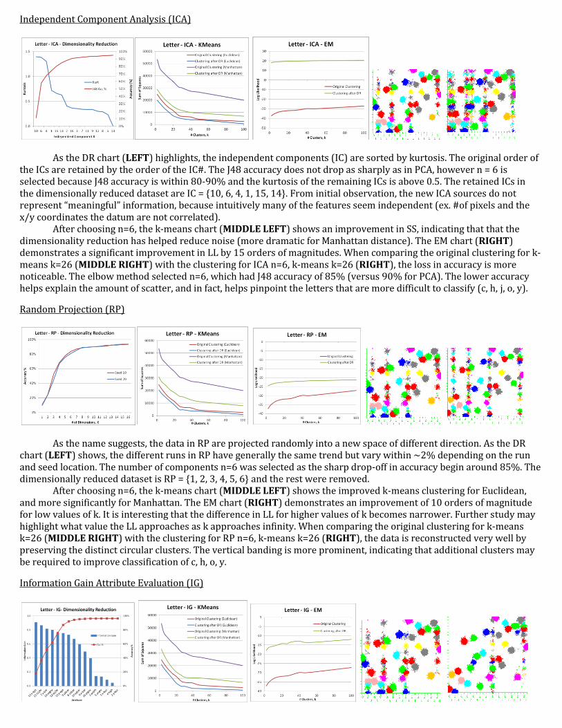
As the DR chart (LEFT) highlights, the independent components (IC) are sorted by kurtosis. The original order of the ICs are retained by the order of the IC#. The J48 accuracy does not drop as sharply as in PCA, however n = 6 is selected because J48 accuracy is within 80-90% and the kurtosis of the remaining ICs is above 0.5. The retained ICs in the dimensionally reduced dataset are IC = {10, 6, 4, 1, 15, 14}. From initial observation, the new ICA sources do not represent “meaningful” information, because intuitively many of the features seem independent (ex. #of pixels and the x/y coordinates the datum are not correlated).

After choosing n=6, the k-means chart (MIDDLE LEFT) shows an improvement in SS, indicating that that the dimensionality reduction has helped reduce noise (more dramatic for Manhattan distance). The EM chart (RIGHT) demonstrates a significant improvement in LL by 15 orders of magnitudes. When comparing the original clustering for k-means k=26 (MIDDLE RIGHT) with the clustering for ICA n=6, k-means k=26 (RIGHT), the loss in accuracy is more noticeable. The elbow method selected n=6, which had J48 accuracy of 85% (versus 90% for PCA). The lower accuracy helps explain the amount of scatter, and in fact, helps pinpoint the letters that are more difficult to classify (c, h, j, o, y).

Random Projection (RP)

As the name suggests, the data in RP are projected randomly into a new space of different direction. As the DR chart (LEFT) shows, the different runs in RP have generally the same trend but vary within ~2% depending on the run and seed location. The number of components n=6 was selected as the sharp drop-off in accuracy begin around 85%. The dimensionally reduced dataset is RP = {1, 2, 3, 4, 5, 6} and the rest were removed.

After choosing n=6, the k-means chart (MIDDLE LEFT) shows the improved k-means clustering for Euclidean, and more significantly for Manhattan. The EM chart (RIGHT) demonstrates an improvement of 10 orders of magnitude for low values of k. It is interesting that the difference in LL for higher values of k becomes narrower. Further study may highlight what value the LL approaches as k approaches infinity. When comparing the original clustering for k-means k=26 (MIDDLE RIGHT) with the clustering for RP n=6, k-means k=26 (RIGHT), the data is reconstructed very well by preserving the distinct circular clusters. The vertical banding is more prominent, indicating that additional clusters may be required to improve classification of c, h, o, y.

Information Gain Attribute Evaluation (IG)

As the DR chart (LEFT) shows, the J48 accuracy is very well preserved until n=7, which is also demonstrated through the high values information gain. For dimensionality reduction, n=7 is selected using the elbow method, however it is important to note that this is a higher number of components than PCA, ICA and RP which may account for some differences in accuracy. Also, since J48 decision trees use information gain in the algorithm, it is expected that IG will perform best of the 4 methods. The study of ANN will provide some insight on the overall accuracy of IG.

After choosing n=7, the k-means chart (MIDDLE LEFT) shows the largest improvement in SS across both algorithms. The inflections at k=26 and k=40 continue to be interesting, and support the notion that ~15 additional clusters help capture the less distinguishable classes. The EM chart (MIDDLE) demonstrates the same points: improvement in LL and noticeable inflections at k=26 and k=40. When comparing the original clustering for k-means k=26 (MIDDLE RIGHT) with the clustering for IG n=7, k-means k=26 (RIGHT) the scatter significantly reduced. The vertical bands for c and h have disappeared, however the bands for p, y remain.

Adult Income

When the adult income dataset was introduced, the distribution of attributes and output classes were displayed. The data was dimensionally transformed (not reduced) by PCA, ICA, RP & IG and shown in the graphs below. The key observation here is that PCA and ICA required numeric or binary attributes, so the nominal features were converted, resulting in 100+ features. A portion of the features are visualized below, to demonstrate the distributions within the features, and for comparison with RP (which does not transform the data into Gaussians) and IG (which simply re-orders the features by information gain).

PCA ICA RP IG

Principal Component Analysis (PCA)

As the DR chart (LEFT) shows the variance quickly drops to <1 as expected because about 80% of the features

are binary. As the cumulative variance line shows, the large number of attributes means that no single attribute carries a significant portion of the variance (as seen in Dataset 1). Using the elbow method, the J48 decision tree accuracy begins to drop faster around n=50. This also retains ~60% of the variance.

After choosing n=50, the k-means chart (MIDDLE LEFT) shows an improvement in SS for both distance functions. As expected, more improvement is seen in Euclidean versus Manhattan (despite the large dimensionality) because the majority of features is binary and have maximum values of 1 (as opposed to max value of 15 for Dataset 1). The EM chart (MIDDLE) demonstrates interesting behavior, because EM has negative effects for k<50. It appears as though LL continues to improve beyond k=100, which makes sense given the 107 PCs and 2 output classes. When comparing the original clustering for k-means k=30 (MIDDLE RIGHT) with the clustering for PCA n=50, k-means k=30 (RIGHT) the same 7 clusters appear for Class 1 (>$50k). This indicates that, the dimensionality reduction from 107 PCs to 50 PCs retains most of the original information.

Independent Component Analysis (ICA)

The DR chart (LEFT) shows the accuracy drops sharply after independent component IC 50 and a sharp drop in

kurtosis after IC 10; therefore n=50 is selected. After choosing n=50, the k-means chart (MIDDLE LEFT) shows an improvement in SS for both distance

functions, which is more evident for Euclidean distance (as seen in PCA and ICA). The EM chart (MIDDLE) is interesting as the LL is improved after DR, however it is interesting that the LL becomes positive. This suggests the transformation into binary features and into independent components result in probability densities greater than 1. When comparing the original clustering for k-means k=30 (MIDDLE RIGHT) with the clustering for RP n=10, k-means k=30 (RIGHT), the same 7 clusters appear for Class 1 (>$50k). While the “meaning” of the clusters is not intuitive, it is interesting that similar clusters are found. Some insight into these 7 clusters are provided in the conclusion of this section, however further analysis may be needed.

Random Projection (RP)

The DR chart (LEFT) shows the sporadic accuracy performance based on run and seed location, as expected. It is

suggested to perform many runs to select the number of components based on the general performance of RP. Based on the chart, n=10 was selected as all runs perform well. Note that the dimensionality reduction is ~30% as compared with ~50% in PCA and ICA.

After choosing n=10, the k-means chart (MIDDLE LEFT) shows an improvement in SS for both distance functions (more dramatically for Euclidean since the binary features make distances smaller). The EM chart (MIDDLE) behaves as expected (as compared with PCA which had lower LL for k<50) because EM is based on probabilities and the binary attributes will have high probabilities per classification as compared with the numeric features in Dataset 1. When comparing the original clustering for k-means k=30 (MIDDLE RIGHT) with the clustering for ICA n=50, k-means k=30 (RIGHT), again the same 7 clusters appear for Class 1 (>$50k). The clustering is improved from the original dataset, however the clusters are less distinct and there are more incorrect instances than in PCA and ICA.

Information Gain Attribute Evaluation (IG)

The DR chart (LEFT) shows that 7 features have info gain of 0.08, and the accuracy elbow occurs at n=5 and 85%.

Observing that the information gain of components 5, 6 & 7 and the accuracy change minimally, n=5 is selected. Looking deeper, the 3 components are education, education (years) and occupation, which intuitively are highly correlated (ex.

an engineer will not have less than a university education, or less than 10 years of total education). This suggests there is a high level of overlap between these features, and the cumulative information gain is marginal.

After choosing n=5, the k-means chart (MIDDLE LEFT) shows little improvement in SS for both distance functions, relative to the improvement seen in PCA, ICA & RP. This suggests that the 5 remaining attributes are responsible for the majority of the instance differences. The EM chart (MIDDLE) however, has significant improvement indicating that the removal of 9 attributes improved the likelihood of instances belonging to a particular cluster. When comparing the original clustering for k-means k=30 (MIDDLE RIGHT) with the clustering for IG n=5, k-means k=30 (RIGHT), 7 clusters appear for Class 1 (>$50k)although 4 are more prominent than the other 3. This is likely due to the removal of ~60% of features (compared with 30-50% for the other methods).

Iterations and Clock Time

Letter Recognition Adult Income

The graphs above depict the number of iterations and log clock time required for each clustering run based on the number of clusters. In general, EM (dashed lines) required more iterations and longer time than k-means. For both algorithms, as a function of k clusters, notice the time does not increase smoothly. This is largely because the number of iterations is highly sensitive to k and can significantly extend the run duration.

For Letter Recognition, there is a drop in iterations and time almost consistently at k=26, which coincidentally matches the number of classes. Through the concept of simplicity via Occam’s Razor, this suggests that the methods converge sooner when the number of clusters are “intuitive”. Similarly, for Adult Income, the number of iterations peak around k=10, and lower again close to the intuitive number of clusters k=14 to k=28. Also note that PCA and ICA are much higher in clock time because the number of features grew to 100+ when converting the nominal features to binary.

Conclusion

For Letter Recognition, the re-clustering after DR was performed using k=26 to compare with the original clustering. After executing the experiments and analyzing the results, it appears that k=40 may provide additional insight. The explanation for 40 clusters to represent 26 output classes is that some classes are represented by multiple clusters to separate the more clearly identifiable instances from the ones with characteristics that correlate to multiple classes. IG is useful in highlighting the most relevant features, namely: edge count in x, and correlations between pixels in x with respect to y, and pixels in y with respect to x.

For Adult Income, there were some challenges presented when the features needed to be converted to binary for PCA and ICA to work. This creates unintuitive transformations to the features, such as accounting for multiple race features in one principal component (ex. PC3: -0.453Native Country= United-States+0.424Race= Asian-Pac-Islander-0.392Race= White+0.222Native Country= Philippines+0.171Race= Black). This may require the number of attributes per PC to increase from 5 (30% of the features) to a more meaningful number like 30. This also increased the computational requirement for the tests, which is amplified when applying cross-validation as well. The most relevant features, based on IG, were relationship/marital status, capital gain, age and education. However, it is also important to consider the features with the lowest information gain: sex and race. IG has a preference bias for features with the most breadth, however these features very clearly show that white males make up the majority of the >$50k class.

Part 4 & 5: Neural Network Performance

Dimensionality Reduction and Neural Network

The purpose of this part is to run dimensionality reduction on one of the datasets and to observe the effect on the learner. The selected dataset is the Letter Recognition dataset, as the numeric attributes allow for more interesting

observations of the effects of dimensionality reduction and re-clustering in the next section. From Assignment 1, the optimal learner had an input layer of 26 nodes, hidden layer of 21 nodes, output later of 16 nodes, learning rate of 0.3, momentum of 0.2 and 20 iterations (epochs). The accuracy of the learner was 81%, which will be used as a benchmark throughout this section. Since ANN is a lazy learner, it takes much longer per run than with DT, and thus further study is encouraged to observe behavior according to higher iterations.

The chart below (LEFT) shows the performance of the learners after DR using each of the 4 algorithms. The chart shows how the learner performs as dimensions are removed from the data, and compares this with the results observed in Part 2&3. The first observation is that ANN naturally performs lower than DT for this dataset (by ~15%), however it is expected that performance will improve for iterations at >500. Another observation is that PCA and ICA, which performed well for J48, also perform best for ANN. If the number of dimensions n was chosen using ANN, it would be at n=7 for PCA, ICA and RP; and n=10 for IG.

Clustering and Neural Network

The purpose of this part is to run clustering algorithms to the dimensionally reduced datasets (via the 4 different methods), and to include the clusters as features for the ANN learner. The chart above (RIGHT) shows the ANN performance for 8 different tests.

The 8 tests are shown in the bar chart above, grouped together by DR method. The 8 tests are 4 separate tests performed for the 2 clustering methods, k-means and EM. For the purpose of this section, the Euclidean distance function is used. As the legend describes, k-means is represented by the 4 left-most bars in the bold colors, and EM is represented by the 4 right-most bars in the faded colors. Each of the 4 colored bars represent the 4 separate tests.

The first of 4 tests applied clustering to the dimensionally transformed data, prior to dimensionality reduction (ie. The datasets contained all 16 dimensions of components from PCA, ICA, RP or IG). Clustering was applied using k=26, and the cluster from these tests was added to each instance as 1 feature in addition to the 16 existing dimensions. This increased the learner performance for all methods by 10%. The second of 4 tests continues from the first test by dimensionally reducing the data based on the elbow method employed in Part 2&3 for comparison (rather than selection based on ANN elbow method). Interestingly, the ANN performance is nearly unchanged for PCA and IG, indicating that the data is re-constructed well. ICA and RP also perform well, considering the Learner Accuracy chart (LEFT) predicts a 60-70% accuracy. The third of 4 tests continues from the second test and includes 10 features from clustering instead of 1. Using the values k = {2, 5, 10, 15, 20, 26, 30, 40, 50, 100} to create 10 clusters, the result is 100% accuracy for all 4 DR algorithms for k-means. Interestingly, when the 5-7 DR components are included for EM, the result is performance as low as 30%, which indicates that the clustering lowers the probabilities of possible classifications. The fourth of 4 tests removes the 5-7 DR components and applies the learner to only the 10 clustered features. The performance is 100% again for k-means clustering, and for EM the performance is similar to the third test, except IG is dramatically improved.

Conclusion

Clustering organizes data in an unsupervised manner and is a useful pre-processing technique. Dimensionality reduction assists in removing non-useful features to improve clustering and learner accuracy. As noted in the Algorithm Implementation, the clustering was implemented applied without isolating the label, which creates a positive bias for including clusters as features, particularly for the third and fourth tests that use 10 cluster features. The analysis still applies, however the absolute results are skewed.

Bibliography

[1] Visual History of the World. Retrieved September 20, 2016. Retrieved from https://ourworldindata.org/slides/world-poverty/

[2] Human Development Index (HDI). Retrieved on September 20, 2016. Retrieved from https://ourworldindata.org/human-development-index/

[3] ICA Plugin for WEKA GUI https://github.com/cgearhart/students-filters/raw/master/StudentFilters.zip