Embed Size (px)
Citation preview
Journal of Machine Learning Research 8 (2007) 2047-2081 Submitted 9/05; Revised 11/06; Published 9/07
Unlabeled Compression Schemes for Maximum Classes∗
Dima Kuzmin [email protected]
Manfred K. Warmuth [email protected]
Computer Science DepartmentUniversity of California, Santa Cruz1156 High StreetSanta Cruz, CA, 95064
Editor: John Shawe-Taylor
AbstractMaximum concept classes of VC dimension d over n domain points have size
( n≤d
), and this is
an upper bound on the size of any concept class of VC dimension d over n points. We give acompression scheme for any maximum class that represents each concept by a subset of up to dunlabeled domain points and has the property that for any sample of a concept in the class, therepresentative of exactly one of the concepts consistent with the sample is a subset of the domainof the sample. This allows us to compress any sample of a concept in the class to a subset of upto d unlabeled sample points such that this subset represents a concept consistent with the entireoriginal sample. Unlike the previously known compression scheme for maximum classes (Floydand Warmuth, 1995) which compresses to labeled subsets of the sample of size equal d, our newscheme is tight in the sense that the number of possible unlabeled compression sets of size at mostd equals the number of concepts in the class.
Keywords: compression schemes, VC dimension, maximum classes, one-inclusion graph
1. Introduction
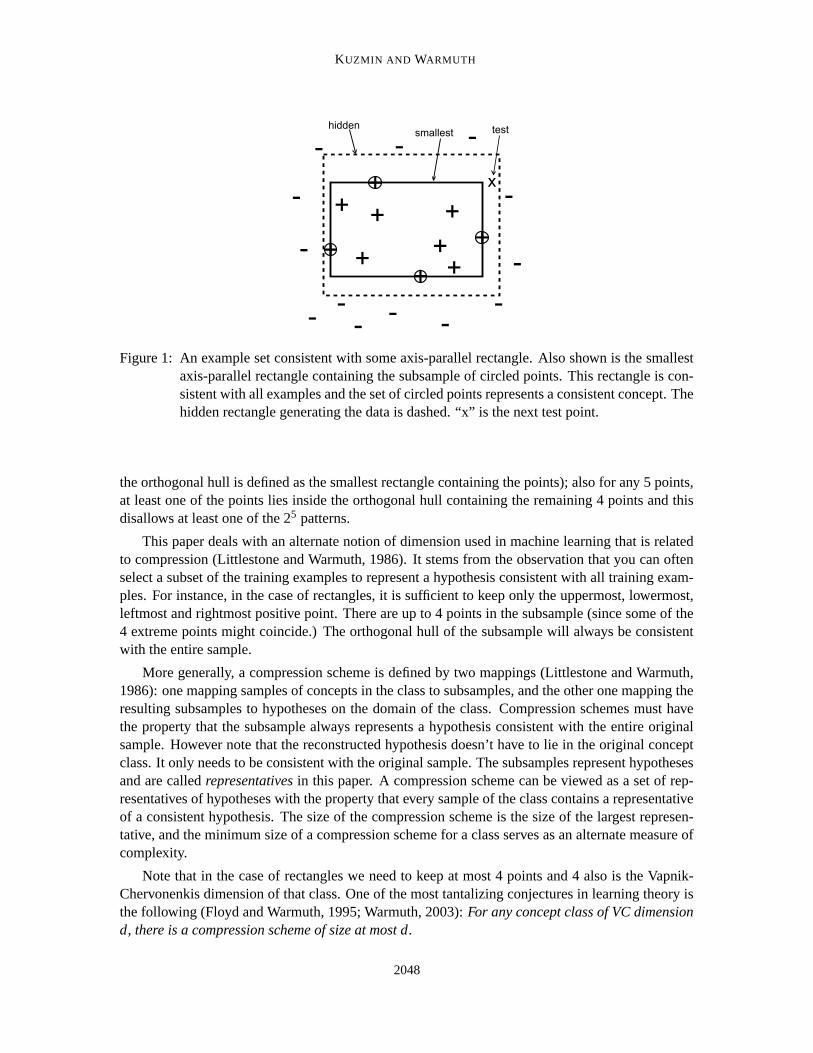
Consider the following type of protocol between a learner and a teacher. Both agree on a domainand a class of concepts (subsets of the domain). For instance, the domain could be the plane and aconcept the subset defined by an axis-parallel rectangle (see Figure 1). The teacher gives a set oftraining examples (labeled domain points) to the learner. The labels of this set are consistent with aconcept (rectangle) that is hidden from the learner. The learner’s task is to predict the label of thehidden concept on a new test point.
Intuitively, if the training and test points are drawn from some fixed distribution, then the la-bels of the test point can be predicted accurately provided the number of training examples is largeenough. The sample size should grow with the inverse of the desired accuracy and with the com-plexity or “dimension” of the concept class. The most basic notion of dimension in this contextis the Vapnik-Chervonenkis dimension. This dimension is the size d of the maximum cardinalitysubset of domain points such that all 2d labeling patterns can be realized by a concept in the class.The VC dimension of axis-parallel rectangles is 4, since it is possible to label any set of 4 pointsin all possible ways as long as no point lies inside the orthogonal hull of the other 3 points (where
∗. Supported by NSF grant CCR CCR 9821087. Some work on this paper was done while the authors were visitingNational ICT Australia.
c©2007 Dima Kuzmin and Manfred K. Warmuth.
KUZMIN AND WARMUTH
+
+
+
++
-
--
-
-
-
-
-
-
-
-
-
-
x
+
+
++
+
hiddensmallest test
Figure 1: An example set consistent with some axis-parallel rectangle. Also shown is the smallestaxis-parallel rectangle containing the subsample of circled points. This rectangle is con-sistent with all examples and the set of circled points represents a consistent concept. Thehidden rectangle generating the data is dashed. “x” is the next test point.
the orthogonal hull is defined as the smallest rectangle containing the points); also for any 5 points,at least one of the points lies inside the orthogonal hull containing the remaining 4 points and thisdisallows at least one of the 25 patterns.
This paper deals with an alternate notion of dimension used in machine learning that is relatedto compression (Littlestone and Warmuth, 1986). It stems from the observation that you can oftenselect a subset of the training examples to represent a hypothesis consistent with all training exam-ples. For instance, in the case of rectangles, it is sufficient to keep only the uppermost, lowermost,leftmost and rightmost positive point. There are up to 4 points in the subsample (since some of the4 extreme points might coincide.) The orthogonal hull of the subsample will always be consistentwith the entire sample.
More generally, a compression scheme is defined by two mappings (Littlestone and Warmuth,1986): one mapping samples of concepts in the class to subsamples, and the other one mapping theresulting subsamples to hypotheses on the domain of the class. Compression schemes must havethe property that the subsample always represents a hypothesis consistent with the entire originalsample. However note that the reconstructed hypothesis doesn’t have to lie in the original conceptclass. It only needs to be consistent with the original sample. The subsamples represent hypothesesand are called representatives in this paper. A compression scheme can be viewed as a set of rep-resentatives of hypotheses with the property that every sample of the class contains a representativeof a consistent hypothesis. The size of the compression scheme is the size of the largest represen-tative, and the minimum size of a compression scheme for a class serves as an alternate measure ofcomplexity.
Note that in the case of rectangles we need to keep at most 4 points and 4 also is the Vapnik-Chervonenkis dimension of that class. One of the most tantalizing conjectures in learning theory isthe following (Floyd and Warmuth, 1995; Warmuth, 2003): For any concept class of VC dimensiond, there is a compression scheme of size at most d.
2048
UNLABELED COMPRESSION SCHEMES FOR MAXIMUM CLASSES
The size of the compression scheme also replaces the VC dimension in the PAC sample sizebounds (Littlestone and Warmuth, 1986; Floyd and Warmuth, 1995; Langford, 2005). However,in the case of compression schemes, the proofs of these bounds are much simpler. There aremany practical algorithms based on compression schemes (e.g., Marchand and Shawe-Taylor, 2002,2003). Also, any algorithm with a mistake bound M leads to a compression scheme of size M (Floydand Warmuth, 1995).
Let’s consider some more illustrative examples of compression schemes. Unions of up to kintervals on the real line form a concept class of VC dimension 2k. We can compress a sample fromthis class to the following set of points: the leftmost “+” point in the sample, the leftmost “−” pointto the right of the last selected point, the leftmost “+” further to the right of the last selected point,and so forth; stop when there are no more points whose label is opposite to the last selected point. Itis easy to see that at most 2k points are kept when the original sample is consistent with a union ofk intervals. Also the labels of the entire original sample can be reconstructed from this subsample.Note that in this case the labels of the subsample are always alternating starting with a “+”. Thusthese labels are redundant and the above scheme can be interpreted as compressing to unlabeledsubsamples of size at most the VC dimension 2k.
Support Vector Machines also lead to a simple labeled compression scheme for halfspaces (setsof the form {x ∈ R
n : w ·x ≥ b}), because only the set of support vectors is needed to reconstructthe hyperplane consistent with the original sample. Of course, the number of support vectors can bequite big. However, it suffices to keep any set of essential support vectors and these sets have sizen + 1, where n is the dimension of the feature space (von Luxburg et al., 2004). Not surprisingly,n+1 is also the VC dimension of arbitrary halfspaces of dimension n. However, the labels of a setof essential support vectors are not redundant and this provides an example of a labeled compressionscheme for halfspaces. There also exists a compression scheme for the same class that compressesto at most n + 1 unlabeled points (Ben-David and Litman, 1998). However this scheme is notconstructive.
The compression scheme conjecture is easily proven for intersection-closed concept classes(Helmbold et al., 1992), which include the class of axis-parallel rectangles as a special case. Moreimportantly, the conjecture was shown to be true for maximum classes. A finite class of VC dimen-sion d over n domain points is maximum if its size is equal to
( n≤d
), which is the upper bound on
the size of any concept class of VC dimension d over n points. An infinite class of VC dimension dis maximum if all restrictions to a finite subset of domain of size at least d are maximum classes ofdimension d.
Of the example concept classes discussed so far, the class of up to k intervals on the real line ismaximum. The class of halfspaces in R
n is not maximum, but it is in fact a union of two classes ofVC dimension n which are “almost maximum”: positive halfspaces and negative halfspaces (Floyd,1989). Positive halfspaces are those that contain the “point” (∞,0, . . . ,0) and negative halfspaces arethose that contain (−∞,0, . . . ,0). Both classes of halfspaces are almost maximum in the sense thatthe restriction to any set of points in general position always produces a maximum class. Finally,the class of axis-parallel rectangles is not maximum since for any five points at least two labelingsare not realizable.
In Floyd and Warmuth (1995) it was shown that for all maximum classes there always existcompression schemes that compress to exactly d labeled examples. In this paper, we give an alter-nate compression scheme for finite maximum classes. Even though we do not resolve the conjecturefor arbitrary classes, we have uncovered a great deal of new combinatorics. Our new scheme com-
2049
KUZMIN AND WARMUTH
x1 x2 x3 x4 r(c)c1 0 0 0 0 /0c2 0 0 1 0 {x3}c3 0 0 1 1 {x4}c4 0 1 0 0 {x2}c5 0 1 0 1 {x3,x4}c6 0 1 1 0 {x2,x3}c7 0 1 1 1 {x2,x4}c8 1 0 0 0 {x1}c9 1 0 1 0 {x1,x3}c10 1 0 1 1 {x1,x4}c11 1 1 0 0 {x1,x2}
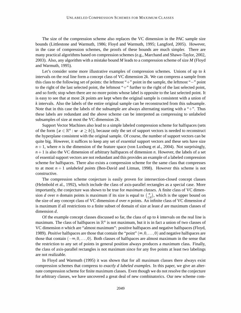
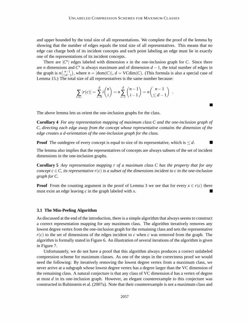
Figure 2: Illustration of the unlabeled compression scheme for some maximum concept class. Therepresentatives for each concept are indicated in the right column and also as the under-lined positions in each row. Suppose the sample is x3 = 1,x4 = 0. The set of conceptsconsistent with that sample is {c2,c6,c9}. The representative of exactly one of theseconcepts is entirely contained in the sample domain {x3,x4}. For our sample this repre-sentative is {x3} which represents c2. So the compressed sample becomes {x3}.
presses any sample consistent with a concept to at most d unlabeled points from the sample. If mis the size of the sample, then there are
( m≤d
)sets of points of size up to d. For maximum classes,
the number of different labelings induced on any set of size m is also( m≤d
). Thus our new scheme
is “tight”. In the previous labeled scheme, the number of possible representatives was much biggerthan the number of concepts.
The new unlabeled scheme also has many interesting combinatorial properties. Let us representfinite classes as a binary table (see Figure 2) where the rows are concepts and the columns are all thepoints in the domain. Our compression scheme represents concepts by subsets of size at most d andfor any k≤ d, the concepts represented by subsets of size up to k will form a maximum class of VCdimension k. Our scheme compresses as follows: After receiving a set of examples, we first restrictourselves to concepts that are consistent with the sample. We then compress to a representativeof a consistent concept that is completely contained in the sample domain (see Figure 2). As ourmain result we will prove that for our choice of representatives, for any sample there always will beexactly one of the consistent concepts whose representative is completely contained in the sampledomain.
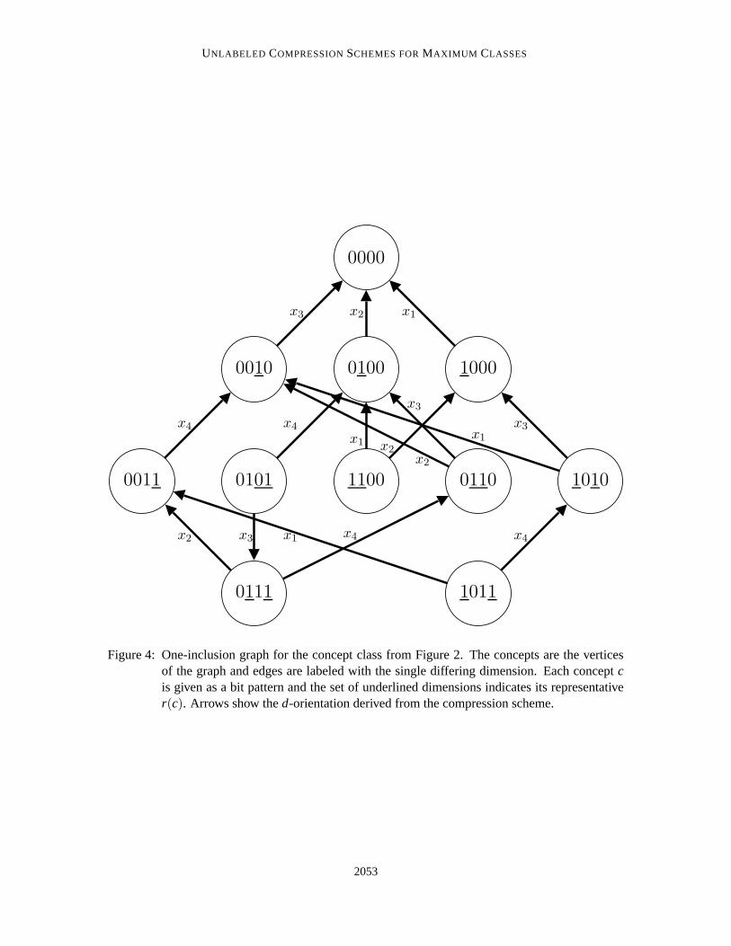
Our new unlabeled compression scheme is connected to a certain undirected graph, called theone-inclusion graph, that characterizes the concept class on a set of example points (Haussler et al.,1994): the vertices are the possible labelings of the example points and there is an edge betweentwo concepts if they disagree on a single point. The edges are naturally labeled by the differingpoints (see Figure 4).
Any prediction algorithm can be used to orient the edges of the one-inclusion graphs as follows.Assume we are given a labeling of some m points x1, . . . ,xm and an unlabeled test point x. If thereis still an ambiguity as to how x should be labeled, then this corresponds to an x-labeled edge in
2050
UNLABELED COMPRESSION SCHEMES FOR MAXIMUM CLASSES
x1 x2 x3 x4
c1 0 0 1 0c2 0 1 0 0c3 0 1 1 0c4 1 0 1 0c5 1 1 0 0c6 1 1 1 0c7 0 0 1 1c8 0 1 0 1c9 1 0 0 0c10 1 0 0 1
,
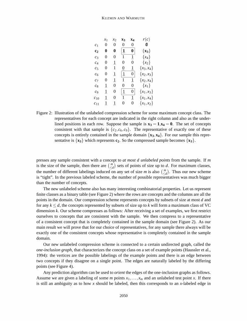
Figure 3: A maximal class of VCdim 2 with 10 concepts. Maximum concept classes of VCdim 2have
( 4≤2
)= 11 concepts (see Figure 2).
one-inclusion graph for the set {x1, . . . ,xm,x}. This edge connects the two possible extensions ofthe labeling of x1, . . . ,xm to the test point x. If the algorithm predicts b, then orient the edge towardthe concept that labels x with bit b.
The vertices in the one-inclusion graph represent the possible labelings of {x1, . . . ,xm,x} pro-duced by the target concepts and if the prediction is averaged over all permutations of the m + 1points, then the probability of predicting wrong is d
m+1 , where d is the out-degree of the target.Therefore the canonical optimal algorithm predicts with an orientation of the one-inclusion graphsthat minimizes the maximum out-degree (Haussler et al., 1994; Li et al., 2002) and in Haussler et al.(1994) it was shown that this outdegree is at most the VC dimension.
How is this all related to our new compression scheme for maximum classes? We show that forany edge labeled with x, exactly one of the two representatives of the incident concepts contains thepoint x. Thus by orienting the edges toward concept that does not have x, we immediately obtainan orientation of the one-inclusion graphs in which all vertices have maximum outdegree at most d(which is the best possible). Again such a d-orientation immediately leads to prediction algorithmswith a worst case expected mistake bound of d
m+1 , where m is the sample size (Haussler et al., 1994),and this bound is optimal1 (Li et al., 2002).
The conjecture whether there always exists a compression scheme of size at most the VC di-mension remains open. For finite domains it clearly suffices to resolve the conjecture for maximalclasses (i.e., classes where adding any concept would increase the VC dimension). We do not knowof any natural example of a maximal concept class that is not maximum or closely related. However,it is easy to find small artificial maximal classes (see Figure 3). We believe that much of the newmethodology developed in this paper for maximum classes will be useful in deciding the generalconjecture in the positive and think that in this paper we made considerable progress toward thisgoal. In particular, we developed a refined recursive structure of finite concept classes and madethe connection to orientations of the one-inclusion graphs. Also, our scheme constructs a certainunique matching that is interesting in its own right.
1. Predicting with a d-orientation of the one-inclusion graphs is also conjectured to lead to optimal algorithms in thePAC model of learning (Warmuth, 2004).
2051
KUZMIN AND WARMUTH
Even though the unlabeled compression schemes for maximum classes are tight in some sense,they are not unique. There is a strikingly simple “peeling algorithm” that always seems to producea valid unlabeled compression scheme for maximum classes: construct the one-inclusion graph forthe domain; iteratively peel off a lowest degree vertex and represent a concept c by the set of datapoints incident to vertex c in the remaining graph when c was removed from the graph (see Figure7 for an example run). However, we have no proof of correctness of this algorithm and the resultingschemes do not have as much recursive structure as the ones produced by our recursive algorithmfor which we have correctness proof. For the small example given in Figure 2, both algorithms canproduce the same scheme.
1.1 Outline of the Paper
Some basic definitions are provided in Section 2. We then define unlabeled compression schemesin Section 3 and characterize the properties of the representation mappings of such schemes andtheir relation to the one-inclusion graph. In this section we also discuss the simple Min-Peeling Al-gorithm in more detail. This algorithm always seems to provide an unlabeled compression schemeeven though we currently do not have a correctness proof for it. Section 4 discusses linear ar-rangements, which are special maximum concept classes, and discuss how to interpret unlabeledcompression schemes for these classes. Next, in Section 5, we briefly summarize the old schemefor maximum classes from Floyd and Warmuth (1995) which compresses to labeled subsamples,whereas ours uses unlabeled ones. The core of the paper is in Section 6, where we give a recursivealgorithm for constructing an unlabeled compression scheme with a detailed proof of correctness.Section 7 contains additional combinatorial lemmas about the structure of maximum classes andunlabeled compression schemes. In Section 8, we discuss how to possibly extend various compres-sion schemes for maximum classes to the more general case of maximal classes. We conclude inSection 9 with a large number of combinatorial open problems that we have encountered in thisresearch.
2. Definitions
Let X be a domain, where we allow X = /0. A concept c is a mapping from X to {0,1}. We can alsoview a concept c as a characteristic function of a subset of dom(c), that is, for any domain pointx∈ dom(c), c(x) = 1 iff x∈ c. A concept class C is a set of concepts with the same domain (denotedas dom(C)). Such a class is represented by a binary table (see Figure 2), where the rows correspondto concepts and the columns to points in dom(C).
Alternatively, C can be represented as a subgraph of the Boolean hypercube of dimension|dom(C)|. Each dimension corresponds to a particular domain point, the vertices are the concepts inC and two concepts are connected with an edge if they disagree on the label of a single point. Thisgraph is called the one-inclusion graph of C (Haussler et al., 1994). Note that each edge is naturallylabeled by the single dimension/point on which the incident concepts disagree (see Figure 4). Theset of incident dimensions of a vertex c in a one-inclusion graph G is the set of dimensions labelingthe edges incident to c. We denote this set as IG(c). Its size equals the degree of c in G.
We denote the restriction of a concept c onto A ⊆ dom(c) as c|A. This concept has domain Aand labels that domain consistently with c. The restriction of an entire class is denoted as C|A. Thisrestriction is produced by simply removing all columns not in A from the table for C and collapsing
2052
UNLABELED COMPRESSION SCHEMES FOR MAXIMUM CLASSES
0000
0010
0011
0100
0101 0110
0111
1000
1010
1011
1100
x3 x2 x1
x4x1
x2 x1
x4
x3
x1
x3x4
x3
x2
x4
x2
Figure 4: One-inclusion graph for the concept class from Figure 2. The concepts are the verticesof the graph and edges are labeled with the single differing dimension. Each concept cis given as a bit pattern and the set of underlined dimensions indicates its representativer(c). Arrows show the d-orientation derived from the compression scheme.
2053
KUZMIN AND WARMUTH
x2 x3 x4
0 0 00 1 00 1 11 0 01 0 11 1 01 1 1
x2 x3 x4
0 0 00 1 00 1 11 0 0
C− x1 Cx1
x1 x2 x3 x4
0 1 0 10 1 1 00 1 1 1
tailx1(C)
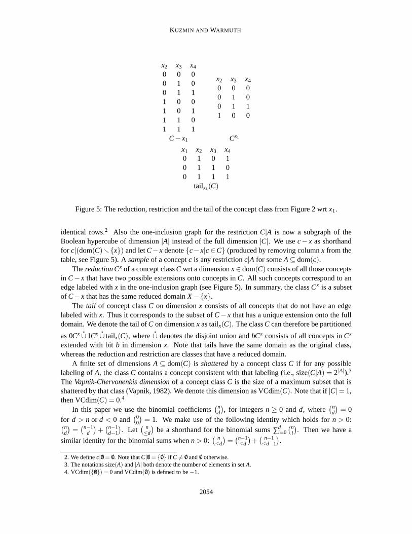
Figure 5: The reduction, restriction and the tail of the concept class from Figure 2 wrt x1.
identical rows.2 Also the one-inclusion graph for the restriction C|A is now a subgraph of theBoolean hypercube of dimension |A| instead of the full dimension |C|. We use c− x as shorthandfor c|(dom(C)r{x}) and let C−x denote {c−x|c ∈C} (produced by removing column x from thetable, see Figure 5). A sample of a concept c is any restriction c|A for some A⊆ dom(c).
The reduction Cx of a concept class C wrt a dimension x∈ dom(C) consists of all those conceptsin C− x that have two possible extensions onto concepts in C. All such concepts correspond to anedge labeled with x in the one-inclusion graph (see Figure 5). In summary, the class Cx is a subsetof C− x that has the same reduced domain X−{x}.
The tail of concept class C on dimension x consists of all concepts that do not have an edgelabeled with x. Thus it corresponds to the subset of C− x that has a unique extension onto the fulldomain. We denote the tail of C on dimension x as tailx(C). The class C can therefore be partitioned
as 0Cx �∪ 1Cx �∪ tailx(C), where�∪ denotes the disjoint union and bCx consists of all concepts in Cx
extended with bit b in dimension x. Note that tails have the same domain as the original class,whereas the reduction and restriction are classes that have a reduced domain.
A finite set of dimensions A ⊆ dom(C) is shattered by a concept class C if for any possiblelabeling of A, the class C contains a concept consistent with that labeling (i.e., size(C|A) = 2|A|).3
The Vapnik-Chervonenkis dimension of a concept class C is the size of a maximum subset that isshattered by that class (Vapnik, 1982). We denote this dimension as VCdim(C). Note that if |C|= 1,then VCdim(C) = 0.4
In this paper we use the binomial coefficients(n
d
), for integers n ≥ 0 and d, where
(nd
)= 0
for d > n or d < 0 and(0
0
)= 1. We make use of the following identity which holds for n > 0:(n
d
)=
(n−1d
)+
(n−1d−1
). Let
( n≤d
)be a shorthand for the binomial sums ∑d
i=0
(ni
). Then we have a
similar identity for the binomial sums when n > 0:( n≤d
)=
(n−1≤d
)+
( n−1≤d−1
).
2. We define c| /0 = /0. Note that C| /0 = { /0} if C 6= /0 and /0 otherwise.3. The notations size(A) and |A| both denote the number of elements in set A.4. VCdim({ /0}) = 0 and VCdim( /0) is defined to be −1.
2054
UNLABELED COMPRESSION SCHEMES FOR MAXIMUM CLASSES
From Vapnik and Chervonenkis (1971) and Sauer (1972) we know that for all concept classeswith VC dimension d: |C| ≤
(|dom(C)|≤d
)(generally known as Sauer’s lemma). A concept class C with
VCdim(C) = d is called maximum (Welzl, 1987) if for all finite subsets Y of the domain dom(C),size(C|Y ) =
(|Y |≤d
). If C is a maximum class with d = VCdim(C), then ∀x∈ dom(C), the classes C−x
and Cx are also maximum classes and have VC dimensions d and d−1, respectively (Welzl, 1987).From this it follows that for finite domains, a concept class C is maximum iff size(C) =
(|dom(C)|≤d
).
A concept class C is called maximal if adding any other concept to C will increase its VCdimension. Any maximum class on a finite domain is also maximal (Welzl, 1987). However, thereexist finite maximal classes, which are not maximum (see Figure 3 for an example).
From now on we only consider finite classes. As our main result we construct an unlabeledcompression scheme for any finite maximum class. The existence of an unlabeled scheme forinfinite maximum classes then follows from a compactness theorem given in Ben-David and Litman(1998). The proof of that theorem is, however, non-constructive.
3. Unlabeled Compression Scheme
Our unlabeled compression scheme for maximum classes represents the concepts as unlabeled sub-sets of dom(C) of size at most d. For any c ∈ C we call r(c) its representative. Intuitively wewant concepts to disagree on their representatives. We say that two different concepts clash wrt r ifc|(r(c)∪ r(c′)) = c′|(r(c)∪ r(c′)).Main definition: A representation mapping r of a maximum concept class C must have the follow-ing two properties:
1. r is a bijection between C and (unlabeled) subsets of dom(C) of size at most VCdim(C) and
2. no two concepts in C clash wrt r.
The following lemma shows how the non-clashing requirement can be used to find a unique repre-sentative for each sample.
Lemma 1 Let r be any bijection between a finite maximum concept class C of VC dimension d andsubsets of dom(C) of size at most d. Then the following two statements are equivalent:
1. No two concepts clash wrt r.
2. For all samples s of a concept from C, there is exactly one concept c ∈ C that is consistentwith s and r(c)⊆ dom(s).
Based on this lemma it is easy to see that a representation mapping r for a maximum conceptclass C defines a compression scheme as follows. For any sample s of C we compress s to theunique representative r(c) such that c is consistent with s and r(c) ⊆ dom(s). Reconstruction iseven simpler, since r is bijective: if s is compressed to the set r(c), then we reconstruct to theconcept c. See Figure 2 for an example of how compression and reconstruction work.Proof of Lemma 1
2⇒ 1 : Proof by contrapositive. Assume ¬1, that is, there ∃c,c′ ∈ C, c 6= c′ s.t. c|r(c)∪ r(c′) =c′|r(c)∪ r(c′). Then let s = c|r(c)∪ r(c′). Clearly both c and c′ are consistent with s andr(c),r(c′)⊆ dom(s). This negates 2.
2055
KUZMIN AND WARMUTH
1⇒ 2 : At a high level, for any sample domain dom(s) there are as many representatives r(c) ⊆dom(s) as there are different samples having that domain. The no clashing condition impliesthat all concepts with representatives in dom(s) are different from each other on dom(s), thusevery sample has to get at least one representative.
For a more detailed proof assume ¬2, that is, there is a sample s for which there are eitherzero or (at least) two consistent concepts c for which r(c)⊆ dom(s). If two concepts c,c′ ∈Care consistent with s and r(c),r(c′) ⊆ dom(s), then c|r(c)∪ r(c′) = c′|r(c)∪ r(c′) (which is¬1). If there is no concept c consistent with s for which r(c)⊆ dom(s), then since
size(C|dom(s)) =
(|dom(s)|≤ d
)= |{c : r(c)⊆ dom(s)}| .
there must be another sample s′ with dom(s′) = dom(s) for which there are two such concepts.So again ¬1 is implied. 2
Once we have a valid representation mapping for some maximum concept class C, we can easilyderive a valid mapping for any restriction of the class C|A by compressing every restricted concept.This is discussed in the following corollary.
Corollary 2 For any maximum class C and A ⊆ dom(C), if r is a representation mapping for Cthen a representation mapping for C|A can be constructed as follows. For any c ∈C|A, let rA(c) bethe representative of the unique concept c′ ∈C, such that c′|A = c and r(c′)⊆ A.
Proof The construction of the mapping for C|A essentially tells us to treat the concept c as a samplefrom C and to compress it. Thus we can apply Lemma 1 to see that rA(c)⊆ A is always uniquely de-fined. Now we need to show that rA satisfies the conditions of the Main Definition. Since the repre-sentatives rA(c) are subsets of A, the non-clashing property for the representation mapping rA for C|Afollows from the non-clashing condition for r for C. The bijection property follows from a countingargument like the one used in the proof of Lemma 1, since size(C|A) = size({r(c) s.t. r(c)⊆ A}).
The following lemmas and corollaries will be stated only for the concept class C itself. However,in light of Corollary 2 they will also hold for all restrictions C|A.
We first show that a representation mapping r for a maximum classes can be used to derive ad-orientation for the one-inclusion graph of the class (i.e., an orientation of the edges such that theoutdegree of every vertex is at most d). As discussed in the introduction such orientations lead to aprediction algorithm with a worst-case expected mistake bound of d
t at trial t.
Lemma 3 For any representation mapping r of a maximum concept class C and the one-inclusiongraph of C, any edge c x— c′ in the graph has the property that its associated dimension x lies inexactly one of the representatives r(c) or r(c′).
Proof Since c and c′ differ only on dimension x and c|r(c)∪ r(c′) 6= c′|r(c)∪ r(c′), x lies in at leastone of r(c),r(c′). Next we will show that x lies in exactly one.
We say an edge charges its incident concept if the dimension of the edge lies in the representativeof this concept. Every edge charges at least one of its incident concepts and each concept c canreceive at most |r(c)| charges. So the number of charges is lower bounded by the number of edges
2056
UNLABELED COMPRESSION SCHEMES FOR MAXIMUM CLASSES
and upper bounded by the total size of all representations. We complete the proof of the lemma byshowing that the number of edges equals the total size of all representatives. This means that noedge can charge both of its incident concepts and each point labeling an edge must lie in exactlyone of the representations of its incident concepts.
There are |Cx| edges labeled with dimension x in the one-inclusion graph for C. Since thereare n dimensions and Cx is always maximum and of dimension d−1, the total number of edges inthe graph is n
( n−1≤d−1
), where n = |dom(C)|, d = VCdim(C). (This formula is also a special case of
Lemma 15.) The total size of all representatives is the same number because:
∑c∈C
|r(c)|=d
∑i=0
i
(ni
)= n
d
∑i=1
(n−1i−1
)= n
(n−1≤ d−1
).
The above lemma lets us orient the one-inclusion graphs for the class.
Corollary 4 For any representation mapping of maximum class C and the one-inclusion graph ofC, directing each edge away from the concept whose representative contains the dimension of theedge creates a d-orientation of the one-inclusion graph for the class.
Proof The outdegree of every concept is equal to size of its representative, which is ≤ d.
The lemma also implies that the representatives of concepts are always subsets of the set of incidentdimensions in the one-inclusion graphs.
Corollary 5 Any representation mapping r of a maximum class C has the property that for anyconcept c ∈C, its representative r(c) is a subset of the dimensions incident to c in the one-inclusiongraph for C.
Proof From the counting argument in the proof of Lemma 3 we see that for every x ∈ r(c) theremust exist an edge leaving c in the graph labeled with x.
3.1 The Min-Peeling Algorithm
As discussed at the end of the introduction, there is a simple algorithm that always seems to constructa correct representation mapping for any maximum class. The algorithm iteratively removes anylowest degree vertex from the one-inclusion graph for the remaining class and sets the representativer(c) to the set of dimensions of the edges incident to c when c was removed from the graph. Thealgorithm is formally stated in Figure 6. An illustration of several iterations of the algorithm is givenin Figure 7.
Unfortunately, we do not have a proof that this algorithm always produces a correct unlabeledcompression scheme for maximum classes. As one of the steps in the correctness proof we wouldneed the following: By iteratively removing the lowest degree vertex from a maximum class, wenever arrive at a subgraph whose lowest degree vertex has a degree larger than the VC dimension ofthe remaining class. A natural conjecture is that any class of VC dimension d has a vertex of degreeat most d in its one-inclusion graph. However, an elegant counterexample to this conjecture wasconstructed in Rubinstein et al. (2007a). Note that their counterexample is not a maximum class and
2057
KUZMIN AND WARMUTH
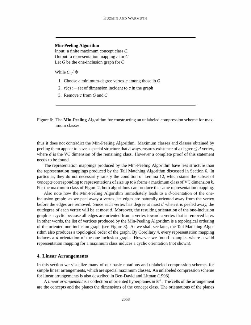
Min-Peeling AlgorithmInput: a finite maximum concept class C.Output: a representation mapping r for CLet G be the one-inclusion graph for C
While C 6= /0
1. Choose a minimum-degree vertex c among those in C
2. r(c) := set of dimension incident to c in the graph
3. Remove c from G and C
Figure 6: The Min-Peeling Algorithm for constructing an unlabeled compression scheme for max-imum classes.
thus it does not contradict the Min-Peeling Algorithm. Maximum classes and classes obtained bypeeling them appear to have a special structure that always ensures existence of a degree≤ d vertex,where d is the VC dimension of the remaining class. However a complete proof of this statementneeds to be found.
The representation mappings produced by the Min-Peeling Algorithm have less structure thanthe representation mappings produced by the Tail Matching Algorithm discussed in Section 6. Inparticular, they do not necessarily satisfy the condition of Lemma 12, which states the subset ofconcepts corresponding to representations of size up to k forms a maximum class of VC dimension k.For the maximum class of Figure 2, both algorithms can produce the same representation mapping.
Also note how the Min-Peeling Algorithm immediately leads to a d-orientation of the one-inclusion graph: as we peel away a vertex, its edges are naturally oriented away from the vertexbefore the edges are removed. Since each vertex has degree at most d when it is peeled away, theoutdegree of each vertex will be at most d. Moreover, the resulting orientation of the one-inclusiongraph is acyclic because all edges are oriented from a vertex toward a vertex that is removed later.In other words, the list of vertices produced by the Min-Peeling Algorithm is a topological orderingof the oriented one-inclusion graph (see Figure 8). As we shall see later, the Tail Matching Algo-rithm also produces a topological order of the graph. By Corollary 4, every representation mappinginduces a d-orientation of the one-inclusion graph. However we found examples where a validrepresentation mapping for a maximum class induces a cyclic orientation (not shown).
4. Linear Arrangements
In this section we visualize many of our basic notations and unlabeled compression schemes forsimple linear arrangements, which are special maximum classes. An unlabeled compression schemefor linear arrangements is also described in Ben-David and Litman (1998).
A linear arrangement is a collection of oriented hyperplanes in Rd . The cells of the arrangement
are the concepts and the planes the dimensions of the concept class. The orientations of the planes
2058
UNLABELED COMPRESSION SCHEMES FOR MAXIMUM CLASSES
0000
0010
0011
0100
0101 0110
0111
1000
1010
1011
1100
x3 x2 x1
x4x1
x2 x1
x4
x3
x1
x3x4
x3
x2
x4
x2
0101 - {x3, x4}
0000
0010
0011
0100
1|0101 0110
0111
1000
1010
1011
1100
x3 x2 x1
x4x1
x2 x1
x4
x3
x1
x3x4
x3
x2
x4
x2
0111 - {x2, x4}
0000
0010
0011
0100
1|0101 0110
2|0111
1000
1010
1011
1100
x3 x2 x1
x4x1
x2 x1
x4
x3
x1
x3x4
x3
x2
x4
x2
0110 - {x2, x3}
0000
0010
0011
0100
1|0101 3|0110
2|0111
1000
1010
1011
1100
x3 x2 x1
x4x1
x2 x1
x4
x3
x1
x3x4
x3
x2
x4
x2
1100 - {x1, x2}
0000
0010
0011
0100
1|0101 3|0110
2|0111
1000
1010
1011
4|1100
x3 x2 x1
x4x1
x2 x1
x4
x3
x1
x3x4
x3
x2
x4
x2
0100 - {x2}
0000
0010
0011
5|0100
1|0101 3|0110
2|0111
1000
1010
1011
4|1100
x3 x2 x1
x4x1
x2 x1
x4
x3
x1
x3x4
x3
x2
x4
x2
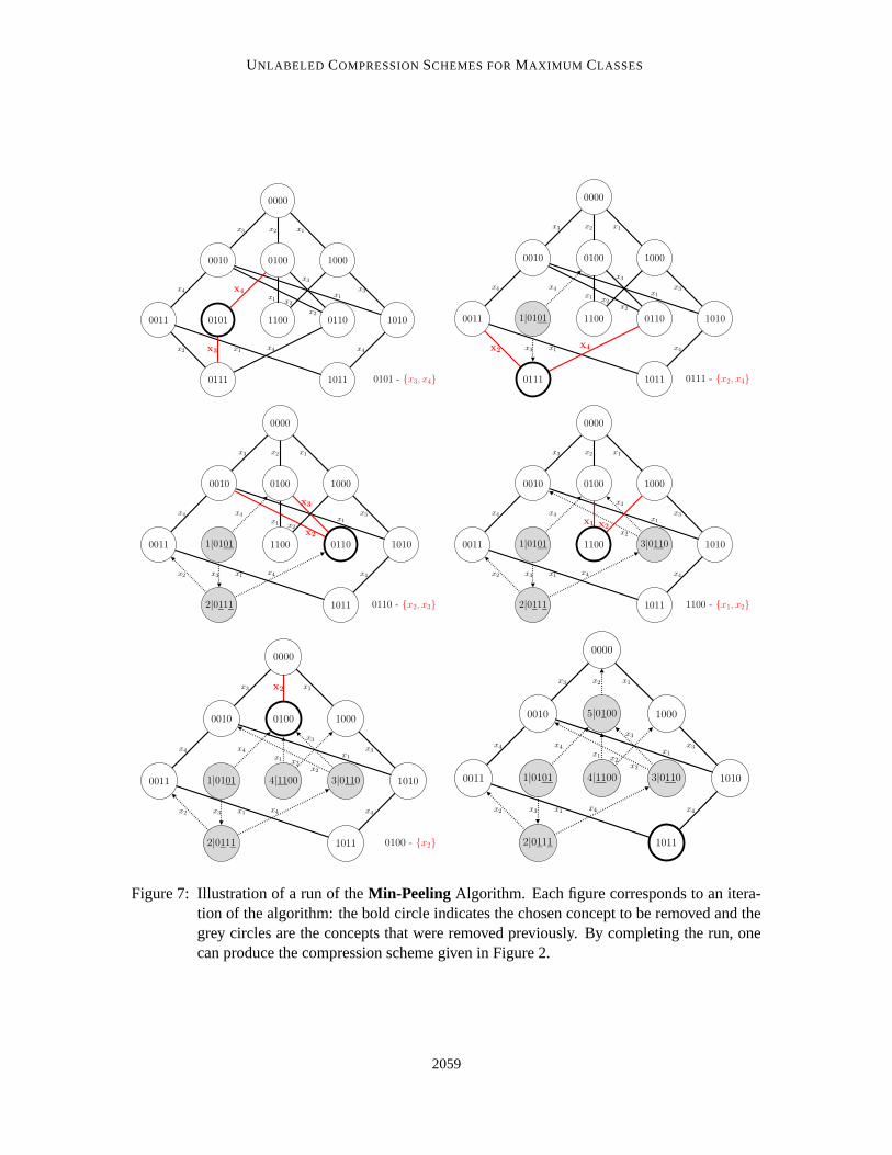
Figure 7: Illustration of a run of the Min-Peeling Algorithm. Each figure corresponds to an itera-tion of the algorithm: the bold circle indicates the chosen concept to be removed and thegrey circles are the concepts that were removed previously. By completing the run, onecan produce the compression scheme given in Figure 2.
2059
KUZMIN AND WARMUTH
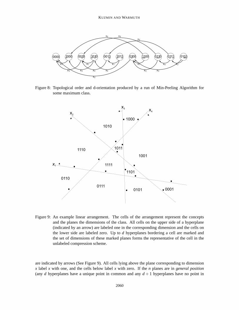
Figure 8: Topological order and d-orientation produced by a run of Min-Peeling Algorithm forsome maximum class.
x1
x3
x4
1010
1110
0110
01110101
1101
1000
1001
0001
1011
1111
x2
Figure 9: An example linear arrangement. The cells of the arrangement represent the conceptsand the planes the dimensions of the class. All cells on the upper side of a hyperplane(indicated by an arrow) are labeled one in the corresponding dimension and the cells onthe lower side are labeled zero. Up to d hyperplanes bordering a cell are marked andthe set of dimensions of these marked planes forms the representative of the cell in theunlabeled compression scheme.
are indicated by arrows (See Figure 9). All cells lying above the plane corresponding to dimensionx label x with one, and the cells below label x with zero. If the n planes are in general position(any d hyperplanes have a unique point in common and any d + 1 hyperplanes have no point in
2060
UNLABELED COMPRESSION SCHEMES FOR MAXIMUM CLASSES
x1
x2
x3
1010
1110
0110
01110101
1101
1000
1001
0001
1011
1111
x4
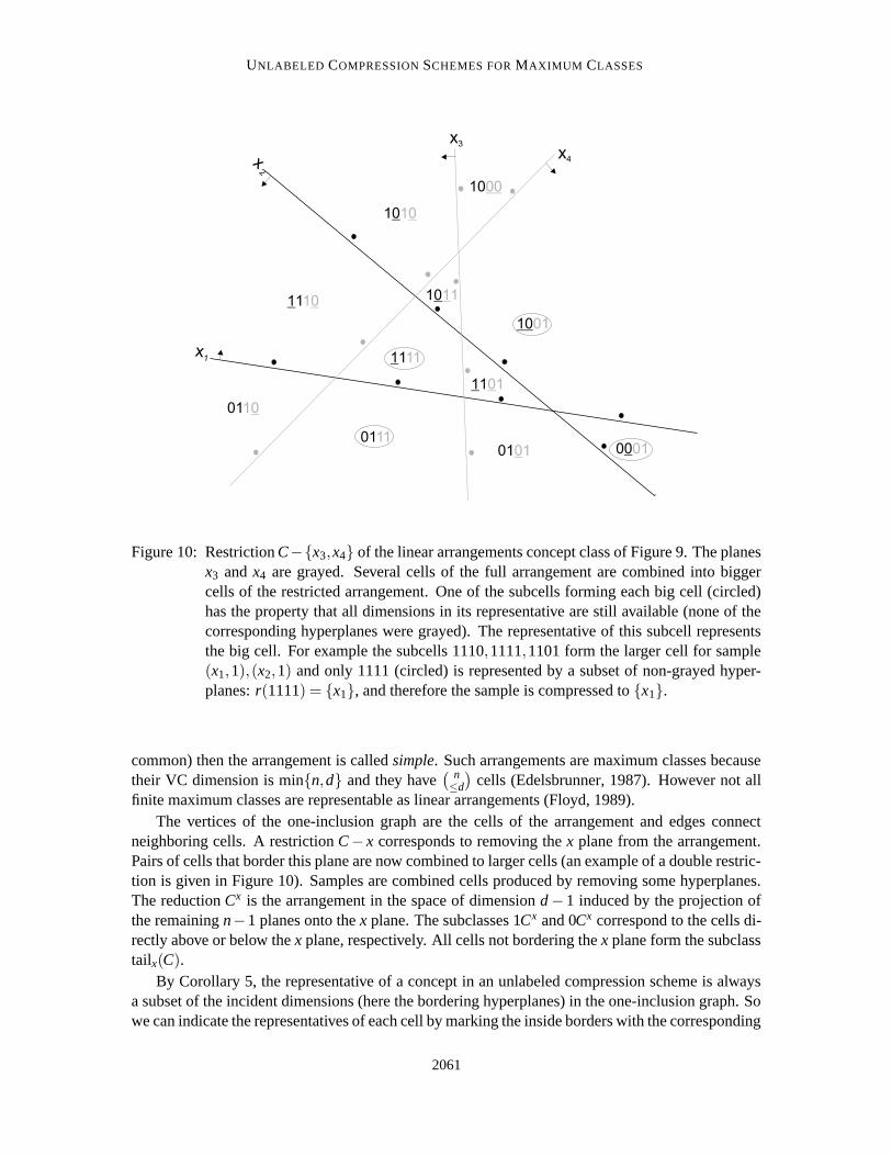
Figure 10: Restriction C−{x3,x4} of the linear arrangements concept class of Figure 9. The planesx3 and x4 are grayed. Several cells of the full arrangement are combined into biggercells of the restricted arrangement. One of the subcells forming each big cell (circled)has the property that all dimensions in its representative are still available (none of thecorresponding hyperplanes were grayed). The representative of this subcell representsthe big cell. For example the subcells 1110,1111,1101 form the larger cell for sample(x1,1),(x2,1) and only 1111 (circled) is represented by a subset of non-grayed hyper-planes: r(1111) = {x1}, and therefore the sample is compressed to {x1}.
common) then the arrangement is called simple. Such arrangements are maximum classes becausetheir VC dimension is min{n,d} and they have
( n≤d
)cells (Edelsbrunner, 1987). However not all
finite maximum classes are representable as linear arrangements (Floyd, 1989).The vertices of the one-inclusion graph are the cells of the arrangement and edges connect
neighboring cells. A restriction C− x corresponds to removing the x plane from the arrangement.Pairs of cells that border this plane are now combined to larger cells (an example of a double restric-tion is given in Figure 10). Samples are combined cells produced by removing some hyperplanes.The reduction Cx is the arrangement in the space of dimension d− 1 induced by the projection ofthe remaining n−1 planes onto the x plane. The subclasses 1Cx and 0Cx correspond to the cells di-rectly above or below the x plane, respectively. All cells not bordering the x plane form the subclasstailx(C).
By Corollary 5, the representative of a concept in an unlabeled compression scheme is alwaysa subset of the incident dimensions (here the bordering hyperplanes) in the one-inclusion graph. Sowe can indicate the representatives of each cell by marking the inside borders with the corresponding
2061
KUZMIN AND WARMUTH
neighbouring cells (See Figure 9). Each cell marks at most d bordering hyperplanes and no cellmarks the same set of hyperplanes. The no-clashing condition of our Main Definition means thatany two cells are on opposite sides of at least one hyperplane marked by one of the cells. Also byLemma 3, any boundary shared between any two cells is marked on exactly one side.
We now visualize how we compress a sample, that is, we restate the process described in Figure2 for the special case of linear arrangements. Recall that a sample s corresponds to a combinedcell produced by removing the hyperplanes in dom(c) r dom(s) where each of the original cellscorresponds to a concept consistent with the sample. One (and only one) of the original cells inthe combined cell that corresponds to the sample is marking only hyperplanes from the survivingset dom(s) (circled in Figure 10). We compress the sample to that set of marked dimensions andreconstruct based on the represented original cell. Note that if the selected original cell marks anyplane, then it must always be at the boundary of the combined cell, since cells in the middle do notborder any of the remaining hyperplanes.
It is interesting to observe how our algorithms construct representation mappings for lineararrangements.
Conjecture 1. Sweeping the arrangement with a hyperplane that is not parallel to any plane inthe arrangement produces a compression scheme as follows: as soon as a cell is completely swept,it marks the planes of all bordering currently live cells. The resulting sequential assignments ofrepresentatives to concepts corresponds to a run of the Min-Peeling Algorithm.
In particular we conjecture that sweeping as prescribed iteratively completes minimum degreecells.
The recursive Tail Matching Algorithm of Section 6 chooses some plane x and first finds acompression scheme for the projection Cx of the linear arrangement onto the this plane. Eachprojected cell from Cx corresponds to two cells, one from 0Cx and one from 1Cx. The algorithmuses the scheme for Cx for all concepts in 0Cx, that is, all cells bordering the x plane from below.The sibling cells in 1Cx right above the plane receive the same marks but also an additional markfrom the x plane. The recursive algorithm uses exactly d marks for all vertices in tailx(C) (the cellsnot bordering the x plane). However, this assignment cannot be easily visualized.
Note that one of the planes has the property that the markings produced by the recursive algo-rithm all lie on one side of the plane. We initially conjectured that there always exist representationschemes that place the marks on the same side for all planes. However we found small counterex-amples to this conjecture (not shown).
Simple linear arrangements are known to have the following property: the shortest path betweenany two cells is always equal to the Hamming distance between the cells (Edelsbrunner, 1987).Surprisingly, we were able to show in Lemma 14 that all maximum classes have this property.
5. Comparison with Old Scheme
In the unlabeled compression schemes introduced in this paper, each subset of up to d domainpoints represents a unique concept in the class, and every sample of a concept contains exactly onesubset that represents a concept consistent with the sample. Before we show that there always existunlabeled compression schemes, we present the old compression scheme for maximum classes fromFloyd and Warmuth (1995) in a concise way that brings out the difference between both schemes.
2062
UNLABELED COMPRESSION SCHEMES FOR MAXIMUM CLASSES
In the old scheme every set of exactly d labeled points represents a concept. Let u denotesuch a set of d labeled points. By the properties of maximum classes, the reduction Cdom(u) is amaximum class of VC dimension 0, that is, just a single concept on the domain dom(C)rdom(u).5
Augmenting this concept with any of the 2d labelings of dom(u), leads to a concept in C on the fulldomain. Let cu denote the concept in C represented by the labeled set u in this way.
Note that there are 2d(n
d
)labeled subsets of size d when the domain size is n, and the number of
concepts in the maximum class C is( n≤d
). This means that some concepts have multiple represen-
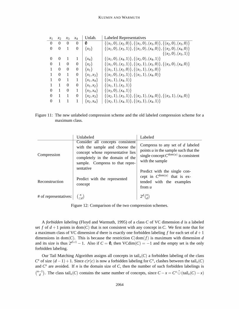
tatives in the old scheme. In Figure 11 we give both compression schemes for the maximum classused in the previous figures.
We first reason that every concept in C is represented by some labeled subset u of the domainof size d. Since the one-inclusion graph for C is connected (see Gurvits, 1997, or Lemma 14 of thispaper), any concept c has an edge along some dimension x. Therefore, c− x lies in Cx. Inductivelywe can find a labeled set v of size d− 1 that represents c− x in Cx. Now let u = v∪{(x,c(x))}.Clearly, cu = c (since Cdom(u) = (Cx)dom(v)).
We still need to show that for every sample s of C with at least d points, there is at least onelabeled subset u of size d that represents a concept consistent with the entire sample. Since therestriction C|dom(s) is a maximum class of VC dimension d, it follows from the previous paragraphthat there is a labeled subset u representing the concept s of C|dom(s). However, u also representsa concept c in C. It suffices to show that u represents the same concept on dom(s) wrt both classesC and C|dom(s).
Assume the concept for C labels some point x in dom(s)r dom(u) with 0 and the concept forC|dom(s) labels this point with 1. Then from the construction of the representations for C it followsthat there are 2d concepts in C that label x with 0 and dom(u) in all possible ways. Similarly thereare 2d concepts in C|dom(s) labeling x with 1. The latter concepts extend to concepts in C andtherefore the d +1 points dom(u)∪{x} are shattered by class C, which is a contradiction.
6. Tail Matching Algorithm for Constructing an Unlabeled Compression Scheme
The unlabeled compression scheme for any maximum class can be found by the recursive algorithmgiven in Figure 13. For any x ∈ dom(C), there are two “copies” of Cx in the original class, onein which the concepts in Cx are extended in the x dimension with label 0 and one with extension(x,1). This algorithm first finds a representation mapping r for Cx to subsets of size up to d−1 ofdom(C)r x. It then uses this mapping for the (x,0) extension and adds x to all the representativesin the other extension. Finally, the algorithm completes r by finding the representatives for tailx(C)via the subroutine given in Figure 14.
For correctness, it suffices to show that the constructed mapping satisfies both conditions of ourMain Definition. We begin with some additional definitions and a sequence of lemmas.
For a∈ {0,1} and c∈C−x, ac denotes a concept formed from c by extending it with (x,a). It isusually clear from the context what the missing x dimension is. Similarly, aCx denotes the conceptclass formed by extending all the concepts in Cx with (x,a). Each dimension x ∈ dom(C) can be
used to split class C into three disjoint sets: C = 0Cx �∪1Cx �∪ tailx(C).
5. Here Cdom(u) is just the consecutive reduction on all d dimensions in dom(u). The result of this operation does notdepend on the order of the reductions (Welzl, 1987).
2063
KUZMIN AND WARMUTH
x1 x2 x3 x4 Unlab. Labeled Representatives0 0 0 0 /0 {(x1,0),(x2,0)},{(x1,0),(x3,0)},{(x2,0),(x3,0)}0 0 1 0 {x3} {(x1,0),(x3,1)},{(x1,0),(x4,0)},{(x2,0),(x4,0)}
{(x2,0),(x3,1)}0 0 1 1 {x4} {(x1,0),(x4,1)},{(x2,0),(x4,1)}0 1 0 0 {x2} {(x1,0),(x2,1)},{(x2,1),(x3,0)},{(x3,0),(x4,0)}1 0 0 0 {x1} {(x1,1),(x2,0)},{(x1,1),(x3,0)}1 0 1 0 {x1,x3} {(x1,0),(x3,1)},{(x1,1),(x4,0)}1 0 1 1 {x1,x4} {(x1,1),(x4,1)}1 1 0 0 {x1,x2} {(x1,1),(x2,1)}0 1 0 1 {x3,x4} {(x3,0),(x4,1)}0 1 1 0 {x2,x3} {(x2,1),(x3,1)},{(x2,1),(x4,0)},{(x3,1),(x4,0)}0 1 1 1 {x2,x4} {(x2,1),(x4,1)},{(x3,1),(x4,1)}
Figure 11: The new unlabeled compression scheme and the old labeled compression scheme for amaximum class.
Unlabeled Labeled
Compression
Consider all concepts consistentwith the sample and choose theconcept whose representative liescompletely in the domain of thesample. Compress to that repre-sentative
Compress to any set of d labeledpoints u in the sample such that thesingle concept Cdom(u) is consistentwith the sample
ReconstructionPredict with the representedconcept
Predict with the single con-cept in Cdom(u) that is ex-tended with the examplesfrom u
# of representatives:( n≤d
)2d
(nd
)
Figure 12: Comparison of the two compression schemes.
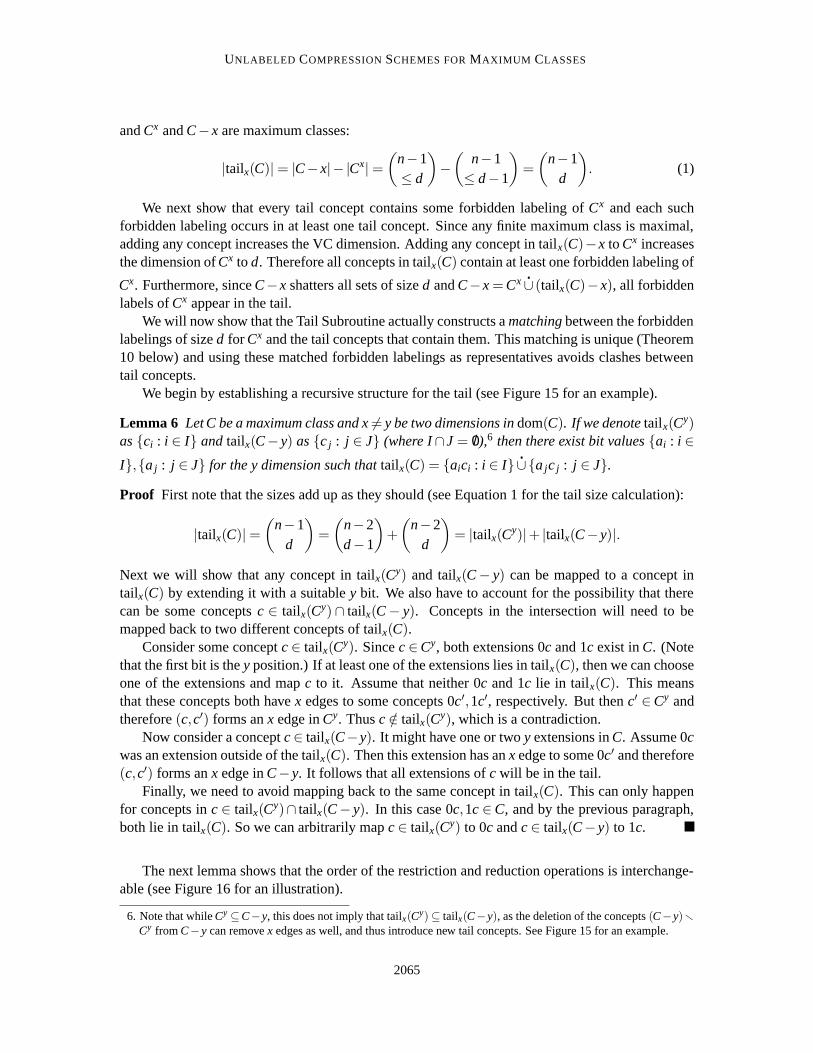
A forbidden labeling (Floyd and Warmuth, 1995) of a class C of VC dimension d is a labeledset f of d + 1 points in dom(C) that is not consistent with any concept in C. We first note that fora maximum class of VC dimension d there is exactly one forbidden labeling f for each set of d +1dimensions in dom(C). This is because the restriction C|dom( f ) is maximum with dimension dand its size is thus 2d+1− 1. Also if C = /0, then VCdim(C) = −1 and the empty set is the onlyforbidden labeling.
Our Tail Matching Algorithm assigns all concepts in tailx(C) a forbidden labeling of the classCx of size (d−1)+1. Since c|r(c) is now a forbidden labeling for Cx, clashes between the tailx(C)and Cx are avoided. If n is the domain size of C, then the number of such forbidden labelings is(n−1
d
). The class tailx(C) contains the same number of concepts, since C− x = Cx �∪ (tailx(C)− x)
2064
UNLABELED COMPRESSION SCHEMES FOR MAXIMUM CLASSES
and Cx and C− x are maximum classes:
|tailx(C)|= |C− x|− |Cx|=(
n−1≤ d
)−
(n−1≤ d−1
)=
(n−1
d
). (1)
We next show that every tail concept contains some forbidden labeling of Cx and each suchforbidden labeling occurs in at least one tail concept. Since any finite maximum class is maximal,adding any concept increases the VC dimension. Adding any concept in tailx(C)−x to Cx increasesthe dimension of Cx to d. Therefore all concepts in tailx(C) contain at least one forbidden labeling of
Cx. Furthermore, since C−x shatters all sets of size d and C−x = Cx �∪ (tailx(C)−x), all forbiddenlabels of Cx appear in the tail.
We will now show that the Tail Subroutine actually constructs a matching between the forbiddenlabelings of size d for Cx and the tail concepts that contain them. This matching is unique (Theorem10 below) and using these matched forbidden labelings as representatives avoids clashes betweentail concepts.
We begin by establishing a recursive structure for the tail (see Figure 15 for an example).
Lemma 6 Let C be a maximum class and x 6= y be two dimensions in dom(C). If we denote tailx(Cy)as {ci : i ∈ I} and tailx(C− y) as {c j : j ∈ J} (where I∩ J = /0),6 then there exist bit values {ai : i ∈I},{a j : j ∈ J} for the y dimension such that tailx(C) = {aici : i ∈ I} �∪{a jc j : j ∈ J}.
Proof First note that the sizes add up as they should (see Equation 1 for the tail size calculation):
|tailx(C)|=(
n−1d
)=
(n−2d−1
)+
(n−2
d
)= |tailx(C
y)|+ |tailx(C− y)|.
Next we will show that any concept in tailx(Cy) and tailx(C− y) can be mapped to a concept intailx(C) by extending it with a suitable y bit. We also have to account for the possibility that therecan be some concepts c ∈ tailx(Cy)∩ tailx(C− y). Concepts in the intersection will need to bemapped back to two different concepts of tailx(C).
Consider some concept c ∈ tailx(Cy). Since c ∈Cy, both extensions 0c and 1c exist in C. (Notethat the first bit is the y position.) If at least one of the extensions lies in tailx(C), then we can chooseone of the extensions and map c to it. Assume that neither 0c and 1c lie in tailx(C). This meansthat these concepts both have x edges to some concepts 0c′,1c′, respectively. But then c′ ∈Cy andtherefore (c,c′) forms an x edge in Cy. Thus c /∈ tailx(Cy), which is a contradiction.
Now consider a concept c ∈ tailx(C−y). It might have one or two y extensions in C. Assume 0cwas an extension outside of the tailx(C). Then this extension has an x edge to some 0c′ and therefore(c,c′) forms an x edge in C− y. It follows that all extensions of c will be in the tail.
Finally, we need to avoid mapping back to the same concept in tailx(C). This can only happenfor concepts in c ∈ tailx(Cy)∩ tailx(C− y). In this case 0c,1c ∈C, and by the previous paragraph,both lie in tailx(C). So we can arbitrarily map c ∈ tailx(Cy) to 0c and c ∈ tailx(C− y) to 1c.
The next lemma shows that the order of the restriction and reduction operations is interchange-able (see Figure 16 for an illustration).
6. Note that while Cy ⊆C−y, this does not imply that tailx(Cy)⊆ tailx(C−y), as the deletion of the concepts (C−y)r
Cy from C− y can remove x edges as well, and thus introduce new tail concepts. See Figure 15 for an example.
2065
KUZMIN AND WARMUTH
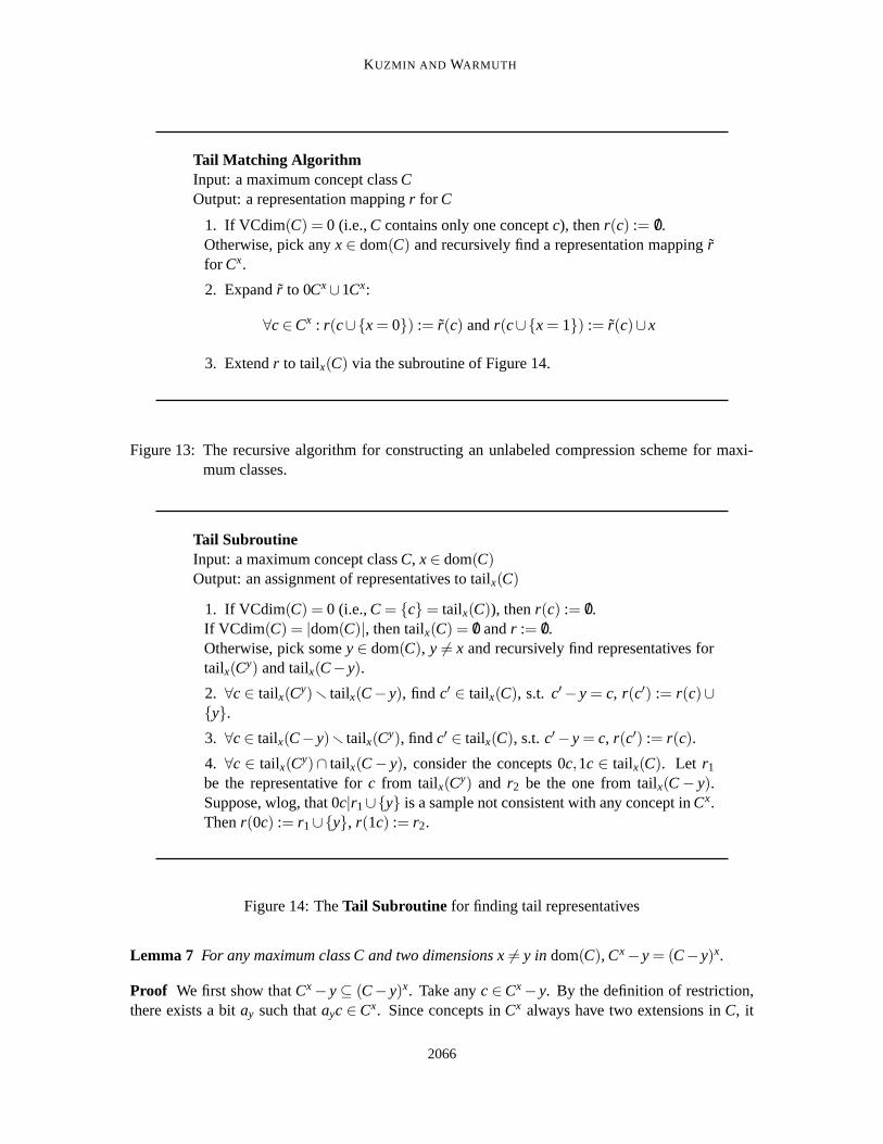
Tail Matching AlgorithmInput: a maximum concept class COutput: a representation mapping r for C
1. If VCdim(C) = 0 (i.e., C contains only one concept c), then r(c) := /0.Otherwise, pick any x ∈ dom(C) and recursively find a representation mapping rfor Cx.
2. Expand r to 0Cx∪1Cx:
∀c ∈Cx : r(c∪{x = 0}) := r(c) and r(c∪{x = 1}) := r(c)∪ x
3. Extend r to tailx(C) via the subroutine of Figure 14.
Figure 13: The recursive algorithm for constructing an unlabeled compression scheme for maxi-mum classes.
Tail SubroutineInput: a maximum concept class C, x ∈ dom(C)Output: an assignment of representatives to tailx(C)
1. If VCdim(C) = 0 (i.e., C = {c}= tailx(C)), then r(c) := /0.If VCdim(C) = |dom(C)|, then tailx(C) = /0 and r := /0.Otherwise, pick some y ∈ dom(C), y 6= x and recursively find representatives fortailx(Cy) and tailx(C− y).
2. ∀c ∈ tailx(Cy)r tailx(C− y), find c′ ∈ tailx(C), s.t. c′− y = c, r(c′) := r(c)∪{y}.3. ∀c ∈ tailx(C− y)r tailx(Cy), find c′ ∈ tailx(C), s.t. c′− y = c, r(c′) := r(c).
4. ∀c ∈ tailx(Cy)∩ tailx(C− y), consider the concepts 0c,1c ∈ tailx(C). Let r1
be the representative for c from tailx(Cy) and r2 be the one from tailx(C− y).Suppose, wlog, that 0c|r1∪{y} is a sample not consistent with any concept in Cx.Then r(0c) := r1∪{y}, r(1c) := r2.
Figure 14: The Tail Subroutine for finding tail representatives
Lemma 7 For any maximum class C and two dimensions x 6= y in dom(C), Cx− y = (C− y)x.
Proof We first show that Cx− y ⊆ (C− y)x. Take any c ∈Cx− y. By the definition of restriction,there exists a bit ay such that ayc ∈ Cx. Since concepts in Cx always have two extensions in C, it
2066
UNLABELED COMPRESSION SCHEMES FOR MAXIMUM CLASSES
x1 x3 x4
0 0 00 1 00 1 11 0 01 1 01 1 10 0 1
x1 x3 x4
0 0 01 0 00 1 00 1 1
x1 x2 x3 x4
0 1 0 1 tailx1(C− x2)0 1 1 0 tailx1(C
x2)0 1 1 1 tailx1(C
x2)
C− x2 Cx2 tailx1(C)
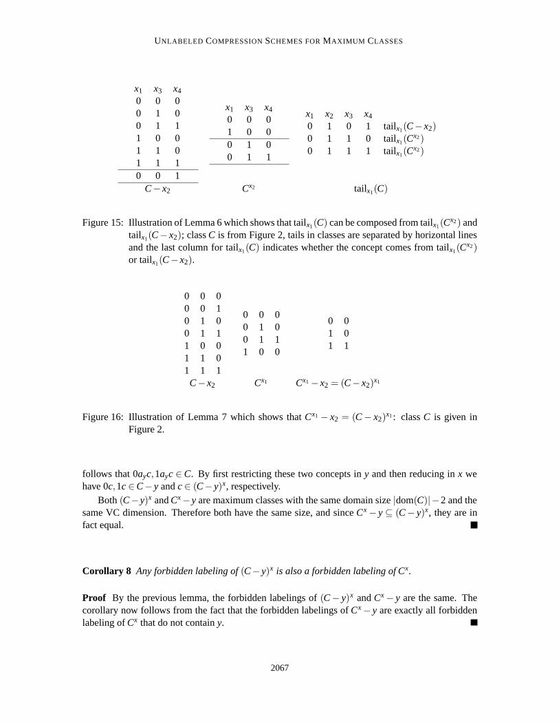
Figure 15: Illustration of Lemma 6 which shows that tailx1(C) can be composed from tailx1(Cx2) and
tailx1(C− x2); class C is from Figure 2, tails in classes are separated by horizontal linesand the last column for tailx1(C) indicates whether the concept comes from tailx1(C
x2)or tailx1(C− x2).
0 0 00 0 10 1 00 1 11 0 01 1 01 1 1
0 0 00 1 00 1 11 0 0
0 01 01 1
C− x2 Cx1 Cx1− x2 = (C− x2)x1
Figure 16: Illustration of Lemma 7 which shows that Cx1 − x2 = (C− x2)x1 : class C is given in
Figure 2.
follows that 0ayc,1ayc ∈C. By first restricting these two concepts in y and then reducing in x wehave 0c,1c ∈C− y and c ∈ (C− y)x, respectively.
Both (C−y)x and Cx−y are maximum classes with the same domain size |dom(C)|−2 and thesame VC dimension. Therefore both have the same size, and since Cx− y ⊆ (C− y)x, they are infact equal.
Corollary 8 Any forbidden labeling of (C− y)x is also a forbidden labeling of Cx.
Proof By the previous lemma, the forbidden labelings of (C− y)x and Cx− y are the same. Thecorollary now follows from the fact that the forbidden labelings of Cx− y are exactly all forbiddenlabeling of Cx that do not contain y.
2067
KUZMIN AND WARMUTH
Lemma 9 If we have a forbidden labeling for Cxy of size d−1, then there exists a bit value for they dimension such that extending this forbidden labeling with this bit results in a forbidden labelingof size d for Cx.
Proof We will establish a bijection between forbidden labelings of Cx of size d that contain y andforbidden labelings of size d− 1 for Cxy. Since Cx is a maximum class of VC dimension d− 1, ithas
(n−1d
)forbidden labelings of size d, one for every set of d dimensions from dom(C)rx. Exactly(n−2
d−1
)of these forbidden labelings contain y and this is also the total number of forbidden labelings
of size d−1 for Cxy.We map the forbidden labelings of size d for Cx that contain y to labelings of size d− 1 by
discarding the y dimension. Assume that a labeling constructed this way is not forbidden in Cxy.Then by extending the concept that contains this labeling with both (y,0) and (y,1) back to Cx, wewill hit the original forbidden set, thus forming a contradiction.
It follows that every forbidden set is mapped to a different forbidden labeling and by the count-ing argument above we see that all forbidden sets are covered. Thus the mapping is a bijection andthe inverse of this mapping proves the lemma.
Theorem 10 Let C be any maximum class C of VC dimension d and domain size n. For any x ∈dom(C) we can construct a bipartite graph between the
(n−1d
)concepts in tailx(C) and the
(n−1d
)
forbidden labelings of size d for Cx with an edge between a concept and a forbidden labeling if thislabeling is contained in the concept. All such graphs have a unique matching.
Proof The proof is an induction on n = |dom(C)| and d. More precisely, we induct on the pairs(n,d) (where n≥ d) in lexicographic order. The minimal element of this order is (0,0).
Note that in the Tail Matching Algorithm 13 we actually stop when n = d, in which case wehave a complete hypercube with no tail and the matching is empty. Also for d = 0, there is a singleconcept which is always in the tail and gets matched to the empty set.
Inductive hypothesis: For any maximum class C, such that (|dom(C|,VCdim(C)) < (n,d) thestatement of the theorem holds.
Inductive step. Let x,y ∈ dom(C) and x 6= y. By Lemma 6, we can compose tailx(C) fromtailx(Cy) and tailx(C−y). Since VCdim(Cx) = d−1 and |dom(C−x)|= n−1,7 then (n−1,d),(n−1,d− 1) < (n,d) and we can use the inductive hypothesis for these classes and assume that thedesired matchings already exist for tailx(Cy) and tailx(C− y).
Now we need to combine these matchings to form a matching for tailx(C). See Figure 14 for adescription of this process. Concepts in tailx(C− y) are matched to forbidden labelings of (C− y)x
of size d. By Lemma 8, any forbidden labeling of (C− y)x is also a forbidden labeling of Cx. Thusthis part of the matching transfers to the appropriate part of tailx(C) without alterations. On theother hand, tailx(Cy) is matched to labelings of size d− 1. We can make them labelings of sized by adding some value for the y coordinate. Some care must be taken here. Lemma 9 tells usthat one of the two extensions will in fact have a forbidden labeling of size d (that includes the ycoordinate). In the case where just one of two possible extensions of a concept in tailx(Cy) is in thetailx(C), there are no problems: the single concept will be the concept of Lemma 9, since the otherconcept lies in Cx and thus does not contain any forbidden labelings. There is also the possibility
7. VCdim(C− x) = d, unless n = d, in which case it would obviously drop by one as well.
2068
UNLABELED COMPRESSION SCHEMES FOR MAXIMUM CLASSES
that both extensions are in tailx(C). From the proof of Lemma 6 we see that this only happens to theconcepts that are in tailx(Cy)∩ tailx(C− y). Then, by Lemma 9, we can figure out which extensioncorresponds to the forbidden labeling involving y and use that for the tailx(Cy) matching. The otherextension will correspond to the tailx(C− y) matching. Essentially, where before Lemma 6 told usto map the intersection tailx(Cy)∩ tailx(C−y) back to tailx(C) by assigning a bit arbitrarily, we nowchoose a bit in a specific way.
So far we have shown that the matching exists. We still need to verify its uniqueness. From anymatching for tailx(C) we will show how to construct matchings for tailx(C− y) and tailx(Cy) withthe property that two different matchings for tailx(C) will disagree with the constructed matchingsfor either tailx(C− y) or tailx(Cy). Now, uniqueness follows by induction.
Consider any concept c in tailx(C), such that c− y ∈ tailx(Cy) r tailx(C− y). Then c− y liesin C− y, but not in tailx(C− y). Therefore c− y must belong to either 0(C− y)x or 1(C− y)x,which means that this concept cannot contain a forbidden set for (C− y)x. We claim that anyforbidden set of c for Cx must contain y. Otherwise such a set would be forbidden for Cx − y,which by Lemma 7 equals (C− y)x. By a similar argument, concepts c ∈ tailx(C), such that c− y ∈tailx(C−y)r tailx(Cy) have to be matched to forbidden sets that do not contain y (since a forbiddenset of size d for Cx that contains y, becomes a forbidden set of size d−1 for Cxy just by removing y,and condition c− y /∈ tailx(Cy) implies that c does not contain any such forbidden sets).
From these two facts it follows that if a concept in tailx(C) is matched to a forbidden set contain-ing y, then c− y ∈ tailx(Cy), and if it is matched to a set not containing y, then c− y ∈ tailx(C− y).We conclude that a matching for tailx(C) splits into a matching for tailx(C− y) and a matching fortailx(Cy). This implies that if there are two matchings for all of tailx(C), then there are either twomatchings for tailx(C− y) or two matchings for tailx(Cy).
Theorem 11 The Tail Matching Algorithm of Figure 13 returns a representation mapping that sat-isfies both conditions of the Main Definition.
Proof Proof by induction on d = VCdim(C). The base case is d = 0: this class has only one conceptwhich is represented by the empty set.
The algorithm recurses on Cx and VCdim(Cx) = d−1. Thus we can assume that it has a correctrepresentation mapping for Cx that uses sets of size at most d−1 for the representatives.
Bijection condition: The representation mapping for C is composed of a bijection between 1Cx
and all sets of size ≤ d containing x, a bijection between 0Cx and all sets of size < d that do notcontain x, and finally a bijection between tailx(C) sets of size equal d that do not contain x.
No clashes condition: By the inductive assumption there cannot be any clashes internally withineach of the subclasses 0Cx and 1Cx, respectively. Clashes between 0Cx and 1Cx cannot occur be-cause such concepts are always differentiated on the x bit and x belongs to all representatives of1Cx. By Theorem 10, we know that concepts in the tail are assigned to representatives that definea forbidden labeling for Cx. Therefore, clashes between tailx(C) and 0Cx, 1Cx are avoided. Finally,we need to argue that there cannot be any clashes internally within the tail. By Theorem 10, thematching between concepts in tailx(C) and forbidden labeling of Cx is unique. So if this matchingresulted in a clash, that is, c1|r1∪ r2 = c2|r1∪ r2, then both c1 and c2 would contain the forbiddenlabelings specified by representative r1 and r2. By swapping the assignment of forbidden labels be-tween c1 and c2 (i.e., c1 is assigned to c1|r2 and c2 to c2|r1) we would create a new valid matching,
2069
KUZMIN AND WARMUTH
thus contradicting the uniqueness of the matching.
Note that by Corollary 4, the unlabeled compression scheme produced by our recursive algorithminduces a d-orientation of the one-inclusion graph: orient each edge away from the concept thatcontains the dimension of the edge in its representative. As was the case for the orientation pro-duced by the Min-Peeling Algorithm, the resulting orientation is acyclic. As a matter of fact atopological order can be constructed by ordering the concepts of C as follows: 0Cx,1Cx, tailx(C).The concept within tailx(C) can be ordered arbitrarily and the concepts within 0Cx and 1Cx areordered recursively based on the topological order for Cx.
7. Miscellaneous Lemmas
We conclude with some miscellaneous lemmas that highlight the combinatorics underlying the un-labeled compression schemes for maximum classes. The first one shows that the representativesconstructed by our Tail Matching Algorithm induce a nesting of maximum classes. This is a specialproperty, because there are cases where the simpler Min-Peeling Algorithm produces a representa-tion mapping that does not have this property (not shown).
Lemma 12 Let C be a maximum concept class with VC dimension d and let r be a representationmapping for C produced by the Tail Matching Algorithm. For 0≤ k≤ d, let Ck = {c∈C s. t. |r(c)| ≤k}. Then Ck is a maximum concept class of VC dimension k.
Proof Proof by induction on d. Base case d = 0: the class has only one concept and the lemmaclearly holds.
The lemma trivially holds for k = 0 or k = d. Otherwise let x ∈ dom(C) be the first dimensionused in the recursion of the Tail Matching Algorithm and assume by induction that the lemma holdsfor Cx. Consider which concepts in C belong to Ck. Clearly none of the concepts in tailx(C) lie inCk because their representatives are of size d > k. From the recursion of the algorithm it followsthat Ck = 0Cx
k ∪ 1Cxk−1, that is, it consists of all concepts in 0Cx with representatives of size ≤ k in
the mapping for Cx, plus all the concepts in 1Cx with representatives of size ≤ k−1 in the mappingfor Cx. By the inductive assumption, Cx
k and Cxk−1 are maximum classes with VC dimension k and
k−1, respectively. Furthermore, the definition of Ck implies that Cxk−1 ⊂Cx
k .
Since |Ck| = |0Cxk |+ |1Cx
k−1| =(n−1≤k
)+
( n−1≤k−1
)=
( n≤k
), the class Ck has the right size and
VCdim(Ck) ≥ k. We still need to show that Ck does not shatter any set of size k + 1. Consider anysuch set that does not contain x. This set would have to be shattered by Ck− x = Cx
k ∪Cxk−1 = Cx
k ,which is impossible. Now consider any set A of size k + 1 that does contain x. All the 1 values forthe x coordinate happen in the 1Cx
k−1 part of Ck. Thus A r x must be shattered by Cxk−1 whose VC
dimension is again one too low.
We actually proved that the Ck produced by the representation mapping of the Tail Matching Al-gorithm always satisfy the recurrence Ck = 0Cx
k ∪ 1Cxk−1. On the other hand there are nestings of
maximum concept classes C0 ⊂ C1 ⊂ . . . ⊂ Cd = C, where Ck has VC dimension k, for which theabove recurrence does not hold (not shown).
Open Problem 1. We do not know whether for any nesting C0 ⊂C1 ⊂ . . . ⊂Cd = C of maximumclasses, where Ck has VC dimension k, there always exists a representation mapping that inducesthis nesting.
2070
UNLABELED COMPRESSION SCHEMES FOR MAXIMUM CLASSES
We now consider the connectivity of the one-inclusion graphs of maximum classes. It wasknown previously that they are connected (Gurvits, 1997). We show in Lemma 14 that the lengthof the shortest path between any two concepts in these graphs is always the Hamming distancebetween the concepts. This property was previously known for the one-inclusion graphs of lineararrangements, which are special maximum classes. The following technical lemma is necessary toprove the property for arbitrary maximum classes.
We use IC(c) to denote the set of dimensions incident to c in the one-inclusion graph for C andlet E(C) denote the set of all edges of the graph.
Lemma 13 For any maximum class C and x ∈ dom(C), restricting wrt x does not change the setsof incident dimensions of concepts in tailx(C), that is, ∀c ∈ tailx(C), IC(c) = IC−x(c− x).
Proof Let (c,c′) be any edge leaving a concept c ∈ tailx(C). By the definition of tailx(C), this edgecannot be an x edge, and therefore c and c′ agree on x and (c− x,c′− x) is an edge in C− x. Itfollows that IC(c)⊆ IC−x(c− x) when c ∈ tailx(C).
If IC(c) is a strict subset of IC−x(c− x) for some c ∈ tailx(C), then the number of edges incidentto tailx(C)− x = (C− x)rCx in C− x is larger than the number of edges incident to tailx(C) in C.The first number is a difference between the sizes of edge sets of the two maximum classes C− xand Cx. Recall that if C is maximum on domain of size n and has VC dimension d, then its edge setE(C) has size n
( n−1≤d−1
)(see proof of Lemma 3 or Lemma 15). Thus the first number is
|E(C− x)|− |E(Cx)|= (n−1)
(n−2≤ d−1
)− (n−1)
(n−2≤ d−2
)
= (n−1)
(n−2d−1
)= d
(n−1
d
).
Furthermore, the second number is the number of edges in C minus the number of intra edgesin 0Cx and 1Cx, respectively, minus the number of cross edges between 0Cx and 1Cx:
|E(C)|−2|E(Cx)|− |Cx| = n
(n−1≤ d−1
)−2(n−1)
(n−2≤ d−2
)−
(n−1≤ d−1
)
= (n−1)
((n−1≤ d−1
)−2
(n−2≤ d−2
))
= (n−1)
((n−2≤ d−1
)−
(n−2≤ d−2
))
= (n−1)
(n−2d−1
)= d
(n−1
d
).
Thus the two numbers are the same and we have a contradiction.
Lemma 14 In the one-inclusion graph for a maximum concept class C, the length of the shortestpath between any two concepts is equal to their Hamming distance.
Proof The proof will proceed by induction on |dom(C)|. The lemma trivially holds when |dom(C)|=0 (i.e., C = /0). Let c1,c2 be any two concepts in a maximum class C of domain size n > 0 and let
2071
KUZMIN AND WARMUTH
x ∈ dom(C). Since C−x is a maximum concept class with a reduced domain size, there is a shortestpath P between c1− x and c2− x in C− x of length equal their Hamming distance. The class C− xis partitioned into Cx and tailx(C)− x. If c1 is the first concept of P in Cx and c2 the last, then byinduction on the maximum class Cx (also of reduced domain size), there is a shortest path betweenc1 and c2 that only uses concepts of Cx. Thus we can assume that P begins and ends with a segmentin tailx(C)− x and has a segment of Cx concepts in the middle, where some of the three segmentsmay be empty.
We partition tailx(C) into tailx=0(C) and tailx=1(C). There are no edges between these twosets because they would have to be x edges. There are also no edges between the restrictionstailx=0(C)− x and tailx=1(C)− x of the two sets, because by Lemma 13 these edges would alsoexist between the original sets tailx=0(C) and tailx=1(C). It follows that any segment of P fromtailx(C)− x must be from the same part of the tail. Also if the initial segment and final segmentof P are both non-empty and from different parts of the tail, then the middle Cx segment cannot beempty.
We can now construct a shortest path P′ between c1 and c2 from the path P. If c1(x) = c2(x) thenwe extend the concepts in P with x = c1(x) to obtain a path P′ between c1 and c2 in C of the samelength. Note that from the above discussion, all concepts in the beginning and ending tail segmentsof P come from the part of the tailx(C) that label x with c1(x) = c2(x). Also for the middle segmentof P we have the freedom to use label c1(x).
If c1(x) 6= c2(x), then P must contain a concept c1 in Cx, because if all concepts in P lied intailx(C)− x then this would imply an edge between a concept in tailx=0(C)− x and a concept intailx=1(C)− x. We now construct a new path P′ in C of length |P|+ 1 which is one more than theHamming distance |P| between c1− x and c2− x: extend the concepts up to c1 in P with label c1(x)on x; then cross to the sibling concept c2 which disagrees with c1 only on its x dimension; finallyextend the concepts in path P from c2 onward with label c2(x) on x.
We already know that the number of vertices and edges in the one-inclusion graph of a maximumclass of domain size n and VC dimension d is
( n≤d
)and n
( n−1≤d−1
), respectively. Since vertices and
edges are hypercubes of dimension 0 and 1, respectively, these bounds are special cases of the belowlemma and corollary, where we bound the number of hypercubes of dimension r, for 0≤ r ≤ d.
Lemma 15 Let C be any class of domain size n and VC dimension d. Then the number of hy-percubes of dimension 0 ≤ r ≤ d which are subgraphs of the one-inclusion graph for C is at most(n
r
)( n−r≤d−r
).
Proof Pick any subset A⊆ dom(C) of size r. Recall that CA consists of all concepts in C|(dom(C)−A) with the property that all 2|A| extensions to the original domain dom(C) are in C. Thus anyconcept in the reduced class CA defines a hypercube of dimension |A| which is a subgraph of theoriginal one-inclusion graph for C. Also from the definition of CA it follows that all hypercubes thatare subgraphs using the dimension set A correspond to a concept in CA. Note that two hypercubesfrom the same CA have no common concepts (vertices), but hypercubes from different restrictionsets of the same size may overlap on their vertex set but they are never identical.
From the above discussion it follows that the total number of hypercubes of dimension r is thetotal size of all CA, where A has size r. Since the reductions CA are classes of domain size n− r andVC dimensions at most d− r, the inequalities of the lemma follow from Sauer’s lemma.
2072
UNLABELED COMPRESSION SCHEMES FOR MAXIMUM CLASSES
Corollary 16 For maximum classes of domain size n and VC dimension d, all d +1 inequalities ofthe previous lemma are tight. Also for any class C of domain size n and VC dimension d, if one ofthe inequalities is tight, then C is maximum and they are all tight.
Proof For maximum classes we have that for any set A of size 0 ≤ r ≤ d, the reduction CA of Cis also a maximum class on domain size n− r and VC dimension d− r (Welzl, 1987; Floyd andWarmuth, 1995). Therefore for maximum classes all inequalities are tight.
Observe that since |C| = |Cx|+ |C− x|, it follows that if Cx and C− x are maximum, then|C|=
( n−1≤d−1
)+
(n−1≤d
)=
( n≤d
)and C is maximum as well.
If the inequality of the previous lemma is tight for some size r, then for all sets of this size, CA
is a maximum class of VC dimension n− r. We will show by the usual double induction on n andd, that in this case C is maximum. Essentially, for Cx the inequality for size r−1 is tight, since forall A containing x, CA = (Cx)(Arx). Furthermore, for C−x the inequality for size r is tight, since forall A not containing x, (C− x)A ⊇CA− x and CA− x is maximum because CA is maximum.
If the following lemma could be proven for any concept class produced by peeling minimumdegree vertices off a maximum class, then this would be sufficient to prove the non-clashing condi-tion for the representation map produced by the Min-Peeling Algorithm. However the current proofonly holds for maximum classes, which is the base case.
Lemma 17 In a maximum class C the labeling of the set of incident dimensions of any concept cuniquely identifies the concept, that is:
∀c′ ∈C : c′ 6= c ⇔ c|IC(c) 6= c′|IC(c). (2)
Proof We employ an induction on |dom(C)|. The base case is |dom(C)| = VCdim(C). In thiscase, C is a complete hypercube. Note that if IC(c) = dom(C), then c|IC(c) = c|dom(C) = c andEquation (2) follows from the uniqueness of each concept. In the hypercube all concepts have thisproperty.
For the general case, if IC(c) 6= dom(C) pick x /∈ IC(c) for which c ∈ tailx(C). We have to showthat ∀c′ 6= c, c|IC(c) 6= c′|IC(c). Consider the maximum concept class C− x and its concept c− x.Because of the reduced domain, we know by induction that
∀c′′ ∈C− x : c′′ 6= c− x ⇔ c− x|IC−x(c− x) 6= c′′|IC−x(c− x).
Since c′′ = c′ − x, for some c′ ∈ C, we can let quantification run over c′ ∈ C and the above isequivalent to
∀c′ ∈C : c′− x 6= c− x ⇔ c− x|IC−x(c− x) 6= c′− x|IC−x(c− x).
Also since c∈ tailx(C) does not have an x edge, ∀c′ ∈C : c′−x 6= c−x is equivalent to ∀c′ ∈C : c′ 6=c and by Lemma 13, IC−x(c−x) = IC(c). This gives us the equivalent statement: ∀c′ ∈C : c′ 6= c ⇔c− x|IC(c) 6= c′− x|IC(c). Finally, since x /∈ IC(c), c− x|IC(c) = c|IC(c) and c′− x|IC(c) = c′|IC(c),giving us Equation (2).
2073
KUZMIN AND WARMUTH
x1 x2 x3 x4 r0 0 0 0 /00 0 1 0 {x3}0 1 0 0 {x2}1 0 0 0 {x1}0 1 1 0 {x2,x3}1 0 1 0 {x1,x3}1 1 0 0 {x1,x2}0 1 1 1 {x1,x4}1 0 1 1 {x2,x4}1 1 0 1 {x3,x4}
1 1 1 1 {x4}
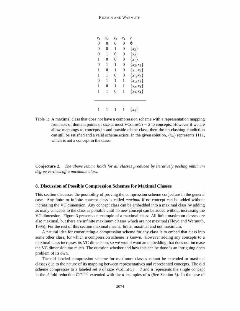
Table 1: A maximal class that does not have a compression scheme with a representation mappingfrom sets of domain points of size at most VCdim(C) = 2 to concepts. However if we areallow mappings to concepts in and outside of the class, then the no-clashing condictioncan still be satisfied and a valid scheme exists. In the given solution, {x4} represents 1111,which is not a concept in the class.
Conjecture 2. The above lemma holds for all classes produced by iteratively peeling minimumdegree vertices off a maximum class.
8. Discussion of Possible Compression Schemes for Maximal Classes
This section discusses the possibility of proving the compression scheme conjecture in the generalcase. Any finite or infinite concept class is called maximal if no concept can be added withoutincreasing the VC dimension. Any concept class can be embedded into a maximal class by addingas many concepts to the class as possible until no new concept can be added without increasing theVC dimension. Figure 3 presents an example of a maximal class. All finite maximum classes arealso maximal, but there are infinite maximum classes which are not maximal (Floyd and Warmuth,1995). For the rest of this section maximal means: finite, maximal and not maximum.
A natural idea for constructing a compression scheme for any class is to embed that class intosome other class, for which a compression scheme is known. However adding any concepts to amaximal class increases its VC dimension, so we would want an embedding that does not increasethe VC dimension too much. The question whether and how this can be done is an intriguing openproblem of its own.
The old labeled compression scheme for maximum classes cannot be extended to maximalclasses due to the nature of its mapping between representatives and represented concepts. The oldscheme compresses to a labeled set u of size VCdim(C) = d and u represents the single conceptin the d-fold reduction Cdom(u) extended with the d examples of u (See Section 5). In the case of
2074
UNLABELED COMPRESSION SCHEMES FOR MAXIMUM CLASSES
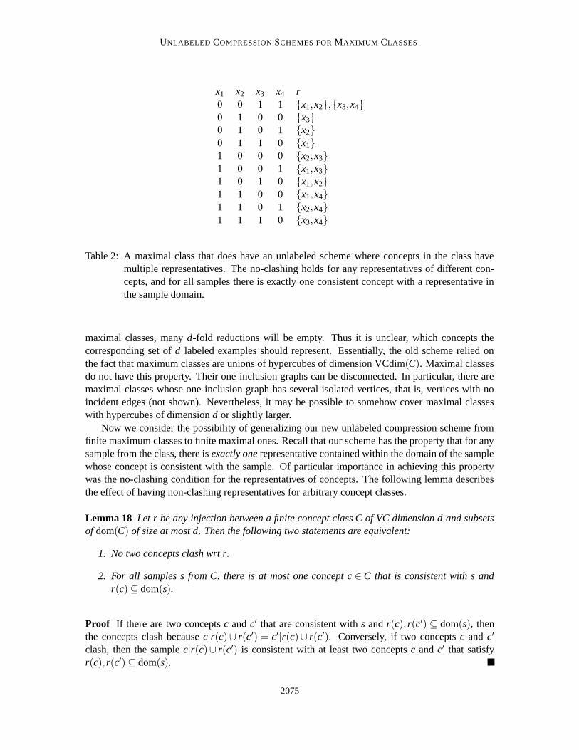
x1 x2 x3 x4 r0 0 1 1 {x1,x2},{x3,x4}0 1 0 0 {x3}0 1 0 1 {x2}0 1 1 0 {x1}1 0 0 0 {x2,x3}1 0 0 1 {x1,x3}1 0 1 0 {x1,x2}1 1 0 0 {x1,x4}1 1 0 1 {x2,x4}1 1 1 0 {x3,x4}
Table 2: A maximal class that does have an unlabeled scheme where concepts in the class havemultiple representatives. The no-clashing holds for any representatives of different con-cepts, and for all samples there is exactly one consistent concept with a representative inthe sample domain.
maximal classes, many d-fold reductions will be empty. Thus it is unclear, which concepts thecorresponding set of d labeled examples should represent. Essentially, the old scheme relied onthe fact that maximum classes are unions of hypercubes of dimension VCdim(C). Maximal classesdo not have this property. Their one-inclusion graphs can be disconnected. In particular, there aremaximal classes whose one-inclusion graph has several isolated vertices, that is, vertices with noincident edges (not shown). Nevertheless, it may be possible to somehow cover maximal classeswith hypercubes of dimension d or slightly larger.
Now we consider the possibility of generalizing our new unlabeled compression scheme fromfinite maximum classes to finite maximal ones. Recall that our scheme has the property that for anysample from the class, there is exactly one representative contained within the domain of the samplewhose concept is consistent with the sample. Of particular importance in achieving this propertywas the no-clashing condition for the representatives of concepts. The following lemma describesthe effect of having non-clashing representatives for arbitrary concept classes.
Lemma 18 Let r be any injection between a finite concept class C of VC dimension d and subsetsof dom(C) of size at most d. Then the following two statements are equivalent:
1. No two concepts clash wrt r.
2. For all samples s from C, there is at most one concept c ∈ C that is consistent with s andr(c)⊆ dom(s).
Proof If there are two concepts c and c′ that are consistent with s and r(c),r(c′) ⊆ dom(s), thenthe concepts clash because c|r(c)∪ r(c′) = c′|r(c)∪ r(c′). Conversely, if two concepts c and c′
clash, then the sample c|r(c)∪ r(c′) is consistent with at least two concepts c and c′ that satisfyr(c),r(c′)⊆ dom(s).
2075
KUZMIN AND WARMUTH
Intuitively, the no-clashing condition causes the representatives to be spread out as much as possiblein an attempt to cover all the samples of concepts in the class. Lemma 18 says that there is at mostone representative whose concept is consistent with the sample. However we also need the at leastone condition, which assures that every sample can be compressed. For maximum classes, the lattercondition was assured by a counting argument: the number of concepts in C|dom(s) and the numberof subsets of size up to d in dom(s) is the same; also all such subsets must represent some conceptand the no-clashing condition assured that these concepts disagreed on dom(s). It follows that foreach sample, there is always at least one representative in its domain that represents a consistentconcept.
There are maximal concept classes of VC dimension d that shatter any set of size d (see Table2). There are |C| representatives in total and this is less than the total number of subsets of size upto d (since C is maximal but not maximum). Therefore, for some domain of size d, there are 2d
concepts but less than that many representatives over the domain.Of course it makes sense to use all subsets of size up to d by assigning some concepts more
than one representative. Note that two representatives of the same concept always clash. However,we still must avoid clashes between representatives of different concepts. A compression schemeis valid if for any sample domain, the number of concepts on the domain equals the number ofconcepts that have at least one representative inside the domain. There exists such a scheme withmultiple representatives for the maximal class of Table 2.
Unfortunately, Table 1 presents a maximal concept class that does not have an unlabeled com-pression scheme of size equal the VC dimension with multiple representatives of concepts in theclass. We checked that for any assignment of multiple representatives to concepts in this class, thereis always some sample that cannot be compressed, that is, there is no representative of a consistentconcept in the sample domain. On the other hand, it is very easy to produce an unlabeled compres-sion scheme for this class if we let some subsets of size at most d represent hypotheses outside ofthe class. Note that in the example of Table 1, the no-clashing condition is satisfied not only for allconcept pairs, but also for the additional hypothesis and any concept in the class.
For the class of Table 1, there also is a compression scheme that maps labeled sets of size equald to just concepts in the class. We do not know whether such schemes exist for arbitrary finiteconcept classes. However, there is an infinite maximum (but not maximal) concept class of VCdimension one with the following property: there is no scheme when labeled points must representconcepts in the class, but there is a scheme when labeled points can represent hypotheses outsideof the class (Eaton, 2005). Also, there is no unlabeled compression scheme for positive halfspacesin R
2 in which the compression sets (of size at most two) represent positive halfspaces (Neylon,2006b).
As has become apparent, there are many variations of compression schemes. We now give aunified notation for all these variations. A compression scheme for a concept class C is essentiallydefined by a mapping f from representatives to hypotheses which are arbitrary subsets of dom(C).Note that the direction of this mapping is opposite to the representation mapping r used for maxi-mum classes.
To define the mapping f , we first choose a set R of representatives which are sets of labeledand/or unlabeled sample points in dom(C). The mapping f maps R to hypotheses, which are arbi-trary subsets of dom(C). Note that f is not required to be injective, allowing for multiple represen-tatives of the same hypothesis. The size of the scheme is the maximum size of any set in R. Themapping f produces a compression scheme as follows:
2076
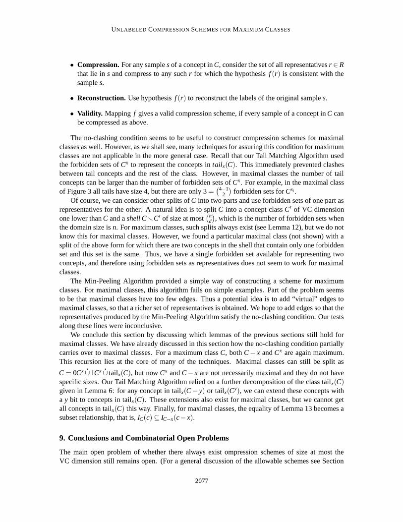
UNLABELED COMPRESSION SCHEMES FOR MAXIMUM CLASSES
• Compression. For any sample s of a concept in C, consider the set of all representatives r ∈ Rthat lie in s and compress to any such r for which the hypothesis f (r) is consistent with thesample s.
• Reconstruction. Use hypothesis f (r) to reconstruct the labels of the original sample s.
• Validity. Mapping f gives a valid compression scheme, if every sample of a concept in C canbe compressed as above.
The no-clashing condition seems to be useful to construct compression schemes for maximalclasses as well. However, as we shall see, many techniques for assuring this condition for maximumclasses are not applicable in the more general case. Recall that our Tail Matching Algorithm usedthe forbidden sets of Cx to represent the concepts in tailx(C). This immediately prevented clashesbetween tail concepts and the rest of the class. However, in maximal classes the number of tailconcepts can be larger than the number of forbidden sets of Cx. For example, in the maximal classof Figure 3 all tails have size 4, but there are only 3 =
(4−12
)forbidden sets for Cxi .
Of course, we can consider other splits of C into two parts and use forbidden sets of one part asrepresentatives for the other. A natural idea is to split C into a concept class C ′ of VC dimensionone lower than C and a shell C rC′ of size at most
(nd
), which is the number of forbidden sets when
the domain size is n. For maximum classes, such splits always exist (see Lemma 12), but we do notknow this for maximal classes. However, we found a particular maximal class (not shown) with asplit of the above form for which there are two concepts in the shell that contain only one forbiddenset and this set is the same. Thus, we have a single forbidden set available for representing twoconcepts, and therefore using forbidden sets as representatives does not seem to work for maximalclasses.
The Min-Peeling Algorithm provided a simple way of constructing a scheme for maximumclasses. For maximal classes, this algorithm fails on simple examples. Part of the problem seemsto be that maximal classes have too few edges. Thus a potential idea is to add “virtual” edges tomaximal classes, so that a richer set of representatives is obtained. We hope to add edges so that therepresentatives produced by the Min-Peeling Algorithm satisfy the no-clashing condition. Our testsalong these lines were inconclusive.
We conclude this section by discussing which lemmas of the previous sections still hold formaximal classes. We have already discussed in this section how the no-clashing condition partiallycarries over to maximal classes. For a maximum class C, both C− x and Cx are again maximum.This recursion lies at the core of many of the techniques. Maximal classes can still be split as
C = 0Cx �∪ 1Cx �∪ tailx(C), but now Cx and C− x are not necessarily maximal and they do not havespecific sizes. Our Tail Matching Algorithm relied on a further decomposition of the class tailx(C)given in Lemma 6: for any concept in tailx(C− y) or tailx(Cy), we can extend these concepts witha y bit to concepts in tailx(C). These extensions also exist for maximal classes, but we cannot getall concepts in tailx(C) this way. Finally, for maximal classes, the equality of Lemma 13 becomes asubset relationship, that is, IC(c)⊆ IC−x(c− x).
9. Conclusions and Combinatorial Open Problems
The main open problem of whether there always exist ompression schemes of size at most theVC dimension still remains open. (For a general discussion of the allowable schemes see Section
2077
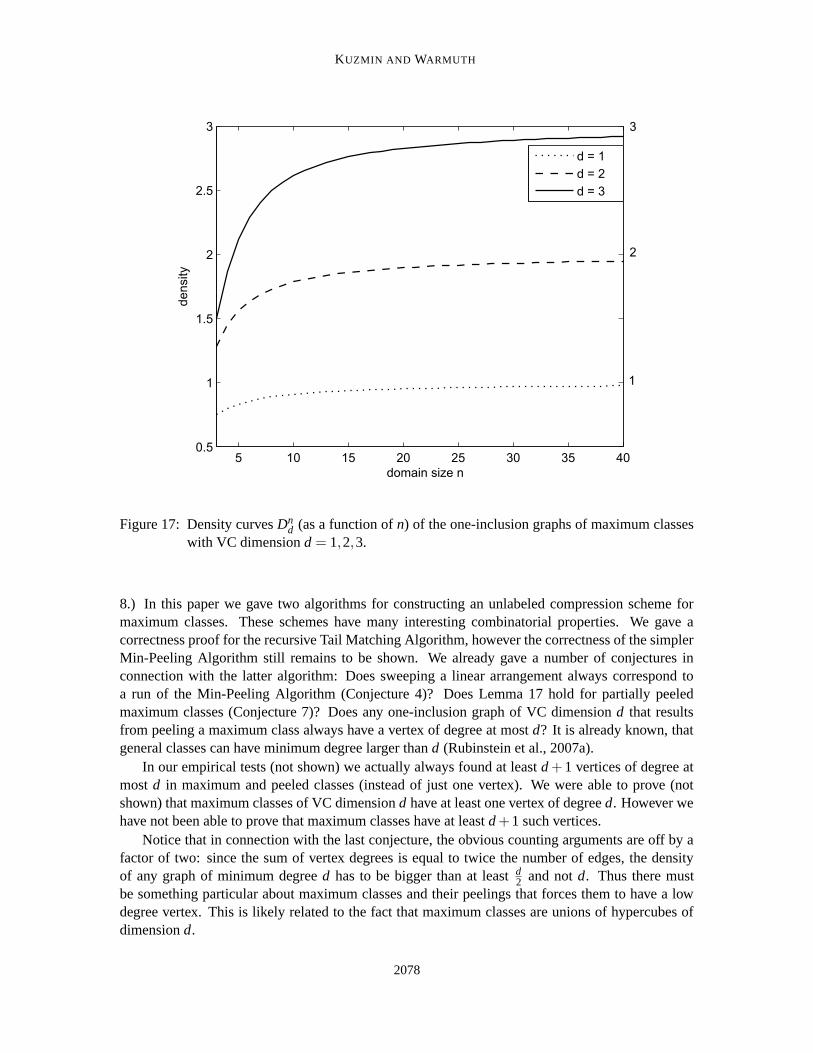
KUZMIN AND WARMUTH
5 10 15 20 25 30 35 400.5
1
1.5
2
2.5
3
domain size n
de
nsity
d = 1
d = 2
d = 3
3
2
1
Figure 17: Density curves Dnd (as a function of n) of the one-inclusion graphs of maximum classes
with VC dimension d = 1,2,3.
8.) In this paper we gave two algorithms for constructing an unlabeled compression scheme formaximum classes. These schemes have many interesting combinatorial properties. We gave acorrectness proof for the recursive Tail Matching Algorithm, however the correctness of the simplerMin-Peeling Algorithm still remains to be shown. We already gave a number of conjectures inconnection with the latter algorithm: Does sweeping a linear arrangement always correspond toa run of the Min-Peeling Algorithm (Conjecture 4)? Does Lemma 17 hold for partially peeledmaximum classes (Conjecture 7)? Does any one-inclusion graph of VC dimension d that resultsfrom peeling a maximum class always have a vertex of degree at most d? It is already known, thatgeneral classes can have minimum degree larger than d (Rubinstein et al., 2007a).
In our empirical tests (not shown) we actually always found at least d + 1 vertices of degree atmost d in maximum and peeled classes (instead of just one vertex). We were able to prove (notshown) that maximum classes of VC dimension d have at least one vertex of degree d. However wehave not been able to prove that maximum classes have at least d +1 such vertices.
Notice that in connection with the last conjecture, the obvious counting arguments are off by afactor of two: since the sum of vertex degrees is equal to twice the number of edges, the densityof any graph of minimum degree d has to be bigger than at least d
2 and not d. Thus there mustbe something particular about maximum classes and their peelings that forces them to have a lowdegree vertex. This is likely related to the fact that maximum classes are unions of hypercubes ofdimension d.
2078
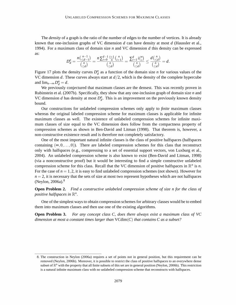
UNLABELED COMPRESSION SCHEMES FOR MAXIMUM CLASSES
The density of a graph is the ratio of the number of edges to the number of vertices. It is alreadyknown that one-inclusion graphs of VC dimension d can have density at most d (Haussler et al.,1994). For a maximum class of domain size n and VC dimension d this density can be expressedas:
Dnd =
n( n−1≤d−1
)( n≤d
) =n∑d−1
i=0i+1
n
( ni+1
)( n≤d
) =∑d
i=1 i(n
i
)( n≤d
) ≤d( n≤d
)( n≤d
) = d.
Figure 17 plots the density curves Dnd as a function of the domain size n for various values of the
VC dimension d. These curves always start at d/2, which is the density of the complete hypercubeand limn→∞ Dn
d = d.We previously conjectured that maximum classes are the densest. This was recently proven in
Rubinstein et al. (2007b). Specifically, they show that any one-inclusion graph of domain size n andVC dimension d has density at most Dn
d . This is an improvement on the previously known densitybound.
Our constructions for unlabeled compression schemes only apply to finite maximum classeswhereas the original labeled compression scheme for maximum classes is applicable for infinitemaximum classes as well. The existence of unlabeled compression schemes for infinite maxi-mum classes of size equal to the VC dimension does follow from the compactness property ofcompression schemes as shown in Ben-David and Litman (1998). That theorem is, however, anon-constructive existence result and is therefore not completely satisfactory.
One of the most important natural infinite classes is the class of positive halfspaces (halfspacescontaining (∞,0, . . . ,0)). There are labeled compression schemes for this class that reconstructonly with halfspaces (e.g., compressing to a set of essential support vectors, von Luxburg et al.,2004). An unlabeled compression scheme is also known to exist (Ben-David and Litman, 1998)(via a nonconstructive proof) but it would be interesting to find a simple constructive unlabeledcompression scheme for this class. Recall that the VC dimension of positive halfspaces in R
n is n.For the case of n = 1,2, it is easy to find unlabeled compression schemes (not shown). However forn = 2, it is necessary that the sets of size at most two represent hypotheses which are not halfspaces(Neylon, 2006a).8
Open Problem 2. Find a constructive unlabeled compression scheme of size n for the class ofpositive halfspaces in R
n.
One of the simplest ways to obtain compression schemes for arbitrary classes would be to embedthem into maximum classes and then use one of the existing algorithms.
Open Problem 3. For any concept class C, does there always exist a maximum class of VCdimension at most a constant times larger than VCdim(C) that contains C as a subset?
8. The construction in Neylon (2006a) requires a set of points not in general position, but this requirement can beremoved (Neylon, 2006b). Moreover, it is possible to restrict the class of positive halfspaces to an everywhere densesubset of R
n with the property that all finite subsets of this set are in general position (Neylon, 2006b). This restrictionis a natural infinite maximum class with no unlabeled compression scheme that reconstructs with halfspaces.
2079
KUZMIN AND WARMUTH
Acknowledgments
We thank Sally Floyd for her personal encouragement and brilliant insights, Sanjoy Dasgupta forthe discussions leading to Lemma 14, and Tyler Neylon for the discussion of unlabeled compressionschemes for positive halfspaces.
References
S. Ben-David and A. Litman. Combinatorial variability of Vapnik-Chervonenkis classes with ap-plications to sample compression schemes. Discrete Applied Mathematics, 86:3 – 25, 1998.
F. Eaton. Private communication, 2005.
H. Edelsbrunner. Algorithms in Combinatorial Geometry, volume 10 of EATCS Monographs onTheoretical Computer Science. Springer-Verlag, Berlin, New York, 1987. ISBN 038713722X.
S. Floyd. Space-bounded learning and the Vapnik-Chervonenkis Dimension (Ph.D). PhD thesis,U.C. Berkeley, December 1989. ICSI Tech Report TR-89-061.
S. Floyd and M. K. Warmuth. Sample compression, learnability, and the Vapnik-Chervonenkisdimension. Machine Learning, 21(3):269–304, 1995.
L. Gurvits. Linear algebraic proofs of VC-dimension based inequalities. In Shai Ben-David, editor,EuroCOLT ’97, Jerusalem, Israel, March 1997, pages 238–250. Springer Verlag, March 1997.
D. Haussler, N. Littlestone, and M. K. Warmuth. Predicting {0,1} functions on randomly drawnpoints. Inform. Comput., 115(2):248–292, 1994.
D. Helmbold, R. Sloan, and M. K. Warmuth. Learning integer lattices. SIAM J. Comput., 21(2):240–266, 1992.
J. Langford. Tutorial on practical prediction theory for classification. Journal of Machine LearningResearch, 6:273–306, 2005.
Y. Li, P. M. Long, and A. Srinivasan. The one-inclusion graph algorithm is near optimal for theprediction model of learning. Transaction on Information Theory, 47(3):1257–1261, 2002.
N. Littlestone and M. K. Warmuth. Relating data compression and learnability. Unpublishedmanuscript, obtainable at http://www.cse.ucsc.edu/˜manfred/pubs/T1.pdf, June 10 1986.
M. Marchand and J. Shawe-Taylor. The Decision List Machine. In Advances in Neural InformationProcessing Systems 15, pages 921–928. MIT-Press, Cambridge, MA, USA, 2003.
M. Marchand and J. Shawe-Taylor. The Set Covering Machine. Journal of Machine LearningResearch, 3:723–746, 2002.
T. Neylon. Sparse Solutions to Linear Prediction Problems. PhD thesis, New York University,Courant Institute of Mathematical Sciences, May 2006a.
T. Neylon. Private communication, 2006b.
2080
UNLABELED COMPRESSION SCHEMES FOR MAXIMUM CLASSES
B.I.P. Rubinstein, P. Bartlett, and J. H. Rubinstein. Shifting: One-inclusion mis-take bounds and sample compression. Technical Report UCB/EECS-2007-86, EECS Department, University of California, Berkeley, Jun 2007a. URLhttp://www.eecs.berkeley.edu/Pubs/TechRpts/2007/EECS-2007-86.html.
B.I.P. Rubinstein, P. L. Bartlett, and J. H. Rubinstein. Shifting, one-inclusion mistake bounds andtight multiclass expected risk bounds. In B. Scholkopf, J. Platt, and T. Hoffman, editors, Advancesin Neural Information Processing Systems 19, pages 1193–1200. MIT Press, Cambridge, MA,2007b.
N. Sauer. On the density of families of sets. Journal of Combinatorial Theory (A), 13:145–147,1972.
V. N. Vapnik. Estimation of Dependences Based on Empirical Data. Springer-Verlag, New York,1982.
V. N. Vapnik and A. Y. Chervonenkis. On the uniform convergence of relative frequencies of eventsto their probabilities. Theory of Probab. and its Applications, 16(2):264–280, 1971.
U. von Luxburg, O. Bousquet, and B. Scholkopf. A compression approach to support vector modelselection. Journal of Machine Learning Research, 5:293–323, April 2004.
M. K. Warmuth. Compressing to VC dimension many points. In Proceedings of the 16th AnnualConference on Learning Theory (COLT 03), Washington D.C., USA, August 2003. Springer.Open problem.
M. K. Warmuth. The optimal PAC algorithm. In Proceedings of the 17th Annual Conference onLearning Theory (COLT 04), Banff, Canada, July 2004. Springer. Open problem.
E. Welzl. Complete range spaces. Unpublished notes, 1987.
2081


![Learned Point Cloud Geometry Compression · (HEVC) intra profile-based image compression [9], [11], [14]. These learned compression schemes have leveraged stacked DNNs to generate](https://img.pdfslide.us/doc/110x75/5f1159a3fa1bcd472d0cb2d7/learned-point-cloud-geometry-compression-hevc-intra-proile-based-image-compression.jpg)