University of. Wisconsin-Madison

IRP Discussion Papers

Anders BjBrklundRopert Moffitt

ESTIMATION ·OF WAGE GAINS .ANDWELFARE GAINS FROMSELF~?ELECTION MODELS

Institute for Research on PovertyDiscussion Paper 735-83

THE ESTIMATION OF WAGE GAINS AND WELFARE GAINSFROM SELF-SELECTION MODELS

Anders BjBrklundThe Industrial Institute for Economic and Social Research and

The Institute for Social Research in Stockholm.

Robert MoffittDepartment 'of Economics

Rutgers University

August 1983

The authors would, like to thank the participants of workshops at theUniversity of Wisconsin and Mathematica Policy Research for comments, aswell as Charles Brown, Randy Brown, Christopher Flinn, and ArthurGoldberger. The research was partially supported by the Institute forResearch on Poverty at the University of Wisconsin.

Abstract

In this paper we consider the basic self-selection model for the

effects of education, training, unions, and other activities on wages.

We show that past models have ignored "heterogeneity of rewards" to the

activity--i.e., differences across individuals in the rate of return to

the activity--as a source of selection bias. We model such heteroge­

neity, show how its presence can be tested, and draw out its implications

for the wage and welfare gains to the activity. An empirical application

provides strong support for such heterogeneity.

THE ESTIMATION OF WAGE GAINS AND WELFARE GAINSFROM SELF-SELECTION MODELS

Economists are often interested in estimating the effect of various

types of choices on wages. In labor economics, applications frequently

have been made in four areas: (1) education, (2) unions, (3) manpower

training, and (4) migration. Researchers on these subjects have become

increasingly concerned with the potential self-selection that may arise,

mainly because the decisions are made by the individuals themselves. In

general, self-selection has been regarded as a disturbing problem for the

issue under examination, for ordinary least squares (OLS) or otherwise

unadjusted estimates of the parameters of interest are biased if self-

selection is present. The usual remedies have been to control for self-

selection either by applying the techniques developed by Maddala and Lee

(1976), Heckman (1978, 1979), and Lee (1979) (see also Barnow, Cain and

Goldberger, 1980), or by trying to avoid the problem by using panel data.

Examples of the first approach are Willis and Rosen (1979) and Kenny et

al. (1979) for education, Lee (1978) for unions, Nakasteen and Zummei

(1980) for migration, and Mallar, Kerachsky, and Thornton (1980) for a

jobs program. Examples of the second approach are Kiefer (1979), Bassi

(forthcoming), and Nickell (1982) for manpower training. 1

In this paper we demonstrate the importance of the selection mecha-

nism per se in these types of problems. Our primary goal is to

demonstrate the implications of interpreting the self-selection model as

a basic model of consumer demand. In the context of the consumer-demand

model we show that selection bias occurs because population heterogeneity

2

causes. different individuals to make different choices--the total popula­

tion of individuals divides itself into participants and nonparticipants

(college attendees and nonattendees, trainees and nontrainees, union

members and nonunion members, etc.). Our most important point is that

population differences arise either because of what we term

"heterogeneity of rewards"--that is, heterogeneity in the rate of return

to the activity--or because of "heterogeneity of costs" to undertake the

activity (both monetary and nonmonetary) or both. 2 We then show that

this distinction has important implications both for the. econometric spe­

cification of the model and for the interpretation of the results--in

particular, for the appropriate estimation of (1) the wage gain to the

activity and (2) the welfare gain of the activity. The presence of costs

creates a wedge between the welfare gain and wage gain. Our initial

point that the selection mechanism is important per se follows from the

fact that the estimation of welfare gains requires structural estimates

of the selection model. Wage gains, even if obtainable by OLS of the

wage equation, are not enough.

The idea of heterogeneity of rewards, which is perhaps our most

important idea, corresponds in regression terms simply to a random coef­

ficients model. We allow the return to education or manpower training.

or some other activity to vary across individuals. We then explicitly

model the endogeneity of education (or the decision to participate in a

training program) by allowing it to be a function of the random coef­

ficient, or the reward. Thus, rather than specifying an ad hoc equation

for education choice, we relate education choice directly to the parame­

ters in the earnings function. This generates a set of cross-equation.

3

constraints between the earnings equation and the education-choice

equation which we impose in the estimation.

The presence of heterogeneity in the return also has strong implica-

tions for public policy, for it implies that those already participating

are, in general, those with the highest return. Expanding the par-

ticipant population--such as by providing educational subsidies or higher

stipends to trainees--draws into the activity those who get less out of.

it. One of the strengths of our model is that it makes this point expli-

cit. Indeed, with our model we can estimate both the mean rewards for

those currently participating as well as the reward for those who would

participate if the costs of participating were lowered.

In the next section we present our model. Then we provide an emp~ri-

cal illustration, using the case of manpower training. Our empirical

results indicate rather dramatically that heterogeneity of rewards are

present. We end with suggestions for future research.

I. HETEROGENEITY IN SELF-SELECTION MODELS

As a point of departure we let the individual maximize the utility

function D(Y. - ~.T), where T is a dummy variable for participation in1. 1.

the activity, ~. denotes the costs of participating in the activity for1.

individual i, and Y denotes the wage. We assume that ~i captures both

monetary costs and a monetized utility component. Let a. be the earnings1.

gain from participation. Thus, the individual participates in the

activity if

where Yi is now interpreted as earnings in the absence of participation.

4

This simple analog with demand theory suggests two sources of heteroge-

neity that might divide the population into participants and

nonparticipants: (1) heterogeneity in rewards (ai) and (2) heteroge­

neity in costs or preferences (~i). In terms of elementary demand theory

it is obvious -that people make different choices if they either face dif-

ferent ".prices" in the budget constraint, ai' or have different utility

functions or different costs, in our case ~i.

Consider now one specification that has been used in the research in

the four areas mentioned at the beginning of this paper: 3

Y. XiS + aT. + £:.1 1 1.

T. 1 if T~ > 01. 1

T. = 0 if T* ~ 01. 1

T~ = W.n + v.1 1. 1.

(1 )

(2 )

(3 )

where Yi is the wage of individual i; Xi is a vector of wage determinants

and S is its associated coefficient vector;_ Ti is a dummy variable for

education (e.g., high school or college), union status, manpower-training

participation, or_residence; Tt is a latent variable determinin~the

dichotomous variable Ti; Wi is a vector of variables affecting Ti and n

is its associated coefficient vector; and £:i and vi are error terms. We

shall formulate our models in terms of a dummy variable, Ti , throughout,

but it will be clear that the analysis would carry through equally if

Ti were continuous.

The model in (1) - (3) implies a specific form of self-selection. It

is obvious that the wage gain, a, is constant and equal for all. In

---- -_.---------~-~----~-----~_.__. __ .- ----~------_.- --------.'

5

terms of demand theory all individuals face the same price of non-

participation. Hence some dispersion or heterogeneity in preferences or

other costs must be present. Therefore we can only interpret W.n and1

Vi in the choice equation as observed and unobserved costs, respectively.

This follows because the specification of the choice equation in terms of

our framework should instead be: 4

*where T. is the net reward. The assumption of homogeneous rewards is in1·

our view rather restrictive. In all the applications we have mentioned

it can be argued. that every individual is unique in terms of his skills

and labor-market situation. Therefore it is reasonable to allow the wage

gains to differ between individuals. A straightforward specification

allowing for both observed and unobserved heterogeneity would be:

(4)

where Z. is a vector of observed variables, 0 is its coefficient vector,1

and u. is an error term. Reformulating the model with (4) gives us the1

following:

Y. XiS + a.T. + E.1 1 1 1

*Ti

= 1 if T. > 01

*T. = 0 if T. .;;; 01 1

*T. = a. - ~.1 1 3.

a. Z.O + u.1 1 3.

.(5 )

(6)

(7 )

(8)

. ~-_ ... _---_._ ..._._~._._..--- ._- ...._.._-_.- .-_.._~.__._--_. ---_..._-~..__ .._ ....~'

6

(9 )

E(v.) = 0~

E(v~) = <12

~ v2E(u.)~

2= <1

U

E(e:.v.)=<1~ ~ e:v

In reduced form the model comes down to: 5

1 (10)

Yi = XiS + e:. , if T. = 0~ ~

*T. 1 , if T. > 0~ ~

0 * 0T. , if T. ,.;;~ ~

* Z.8T. = - W.n + u. - v.~ ~ ~ ~ ~

Here we have let both rewards and costs be a function of a vector of

(11)

(12)

(13 )

observed variables (Z and W respectively) and its own individual error

term. 2The relative importance of 8 and <1 , on the one hand, versus nandu

<1;, on the other hand, provides the empirical basis for judging whether

heterogeneity of rewards or costs is more important. The test for

heterogeneity of rewards is the test of the full model (10)-(13) against

a model with the restrictions <1 u = <1e:u = <1 uv = 0 and 8 = 0 except for a

constant. The test for heterogeneity of costs is the test of the full

model against one with the restrictions a v = <1e:v = <1 uv = O'and n = 0

except for a constant. 6

! 7

This formulation of the problem alters in a rather interesting

fashion the interpretation of the estimated parameters from that usually

given. First, note that there is no longer a single "effect" of the

program since rewards are heterogeneous. Of course, we can speak of a

mean reward, or the reward for an individual with a given characteristics

vector Zio This could be calculated from the estimated parameter vector

o. The "average" reward is, we assume, that to which the usual constant-

parameter estimate in the original equation (1) must correspond. But

note that it could easily be negative, zero, or positive but small.

Since an individual chooses T=l only if the unobserved component u. is~

sufficiently high, there is no reason for the mean reward to be positive.

This obviously has major implications for the interpretation of the wage

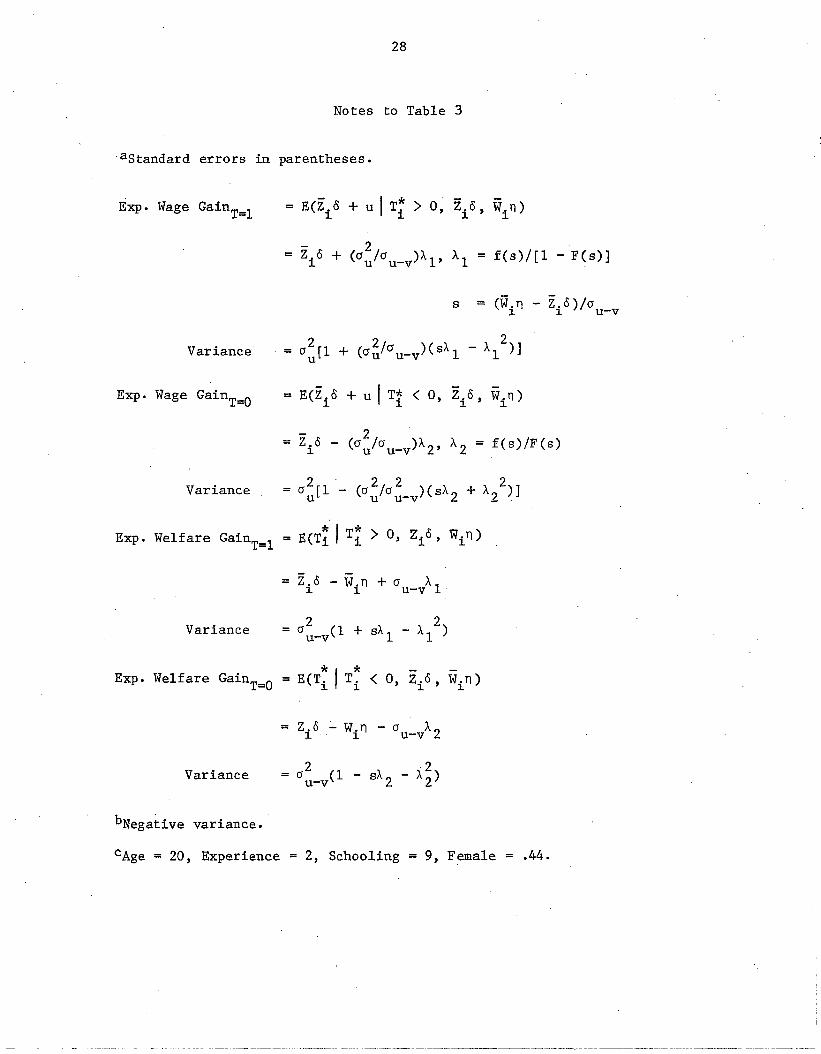
coefficients in previous studies. A more relevant measure of the rate of

return in the mean size of the reward conditional upon choosing T=l:

E(u, I T~ > 0, Z.o, W.n) = Z.o + E(u. u-l - v-l > -Z-I 0 + W-In)1 ~ ~ 1 1 1..L..L ..L ..L

(14 )

= Z.o + (cr /cr )[f(s)/(l-F(s»]1 u,u-v u-v

where s = (-Z.o + W.n)cr ,and f and F are the standard normal density~ 1 u-v

and distribution functions, respectively (we have assumed normality for

the errors). This expression is, we argue, the appropriate measure of

the expected wage gain from the activity T.

*Likewise, note that the T. quantity in equation (6) is simply the1

dollar amount of the net reward (net of costs, that is). At mean values

or any other values of Zi and Wi in the population, it may be negative

even if the reward u. is positive. But we can use it to determine the~

8

*dollar gain from the activity T if an individual undergoes it, for T. is~

just the amount by ~mich income must be reduced in order to leave the

individual indifferent to participation (i.e., at the same utility level

in either case). This value corresponds in consumer-demand theory to the

compensating variation, or "willingness to pay" for the activity. This

consumer-surplus measure can be calculated as:

Zi O -Win +E(ui -vi lUi -vi >-Zio + Win)

(15)

where again s = (-Zio + Win)/cru-v' This welfare gain will equal the ·wage

gain only in the special case cr v = 0uv' n = 0 (i.e., no costs).

Finally, some comments on the role of selection bias in our full

model are warranted. The term selection bias generally refers to the

bias of the 01S estimates of the parameters Sand 0 in the wage equation

that arises if the error terms of these equations are correlated with the

error term of the choice equation. In our full model it appears that if

there is unobserved heterogeneity of rewards, the error term ui will

appear in both equations. Hence selection bias will be present. It is

also important to emphasize that this source of selection bias cannot be

avoided by using panel data and working with first differences--that is,

by formulating the dependent variable as the difference in earnings from

one time period to another. Such a model can be exactly represented by

(10)-(13), with Yi replaced by ~Yi and by reinterpreting €i as the dif-

ference in the level errors in two periods. 7

_.- ._~---~-----_._-~~-------._--------------------------

9

On the other hand, there is also selection bias in the ~ and 0 coef-

ficients if the unobserved costs, v., are correlated with the error term1

in the earnings equation, E •• This is the more usual case of selection1

bias. It will be eliminated by employing a first-difference technique if

vi is correlated only with some permanent component in the level error.

However, note that even if there is no such correlation, the complete

self-selection model (10)-(13) must still be estimated if we want to com-

pute our measure of consumer surplus. Hence we conclude that the self-

selection model is important per se irrespective of any bias of OL8 esti-

mates of the wage equation.

Identification and Estimation

The identification conditions in the full model (10)-(13) are vir-

tually identical to those in the Lee (1979) model and therefore need

little discussion. From our two earnings equations (10) and (11), it is

clear that the coefficient vectors Sand 0 are identified, as are their

. (2 2 2) 2error varlances, 0 + 0 + 0 and 0 •E EU U E

In equation (13) the vector of

parameters n is identified only if there is at least one variable in

Zi that is not in Wi

variance in the·same

(a similar condition2 .

equation, (0 - 2au uv

appears in the Lee model). The

+a2

) is also identified,8 asv

are the covariances between the error in equation (13) and those in

equations (10) and (11). From these composite variances it can be shown

that some normalization is necessary for complete model identification. 9

We have chosen a = 0. 10 Subject to this normalization we can identifyuv

The estimation of the model is also no more or less difficult than

the estimation of the usual self-selection model. The model can be

10

estimated with either. full-information or limited-information techniques.

In the first case the log likelihood function is maximized with respect

to the unknown parameters (S, 0, n, a~, au' a ,a ,a ):v V Eu Ev

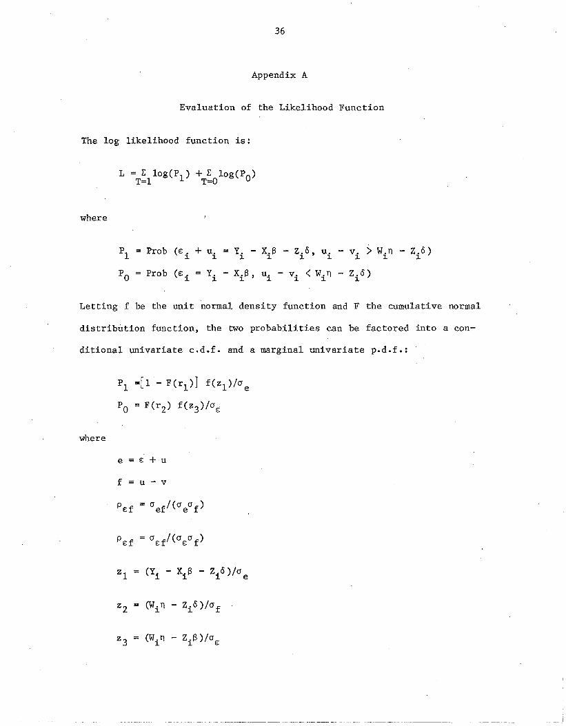
L = E log PI + E log PoT=l T=O

wherell

Prob(£. + u. - Y. - X.S - Z.o, u. - v. > W.n - Z.O)1 1 1 1 1 1 111

The evaluation of PI and Po in terms of normal probabilities and

densities is shown in Appendix A.

In the limited-information case a three-step method can be used (Lee,

1979) • In the first step a reduced-form version of equation (13) is

estimated with probit:

where V. is the union of the vectors Z. and W.. In the second step an1 1 1

augmented earnings equation is estimated with OLS:12

where

11

A2

1Ji1

1Ji2

oe:+u,u-vou-v

o e: ,u-vou-v

The results give consistent estimates of Sand o. In the third step a

modified equation is estimated with probit:

*T. = 1 if T. > 0]. ].

*T. = 0 if T. .. 0]. ].

* ....T. = c(Z.o ) + cW.n +u. - v.

]. ]. ]. ]. ].

where c = 1/0u-v

....Since the coefficient on (Zio) is one over the

standard deviation, the parameter vector n can be obtained by dividing it....

into the probit coefficient vector (en).

This provides estimates of all the coefficients. The composite

variance parameters are also obtainable: 0u-v from the aforementioned

"c" coefficient, 0e:+u,u-v and oe:,u-v thence from the estimates of 1Ji 1 and

2 2and 0e: and 0e:+u by a procedure explained in Lee (1979). (Note that

the last two estimates are not needed for evaluation of the wage gain and

welfare gain.) The underlying variance parameters are then obtainable

from these composites (see n. 9).

The full-information technique is to be preferred for many reasons,

most of all because it is more efficient than the limited-information

~~- ------------~--~--------

12

technique. Also, the cross-equation restrictions for common parameters

are directly imposed in the full-information case. In addition, the OLS

standard errors in the limited-information case are inconsistent; correct

estimates can only be obtained at some effort. This last point is par­

ticularly important for us, for we wish to test the significance of

heterogeneity of rewards and costs. A correct significance test cannot

be performed from the limited-information estimates.

II. AN EMPIRICAL APPLICATION

A. Data and Empirical Specification

To illustrate the model, we have applied it to the government manpower

training program in Sweden. The program provides classroom and other

forms of training in a large variety of fields. The purpose of the

training is to raise the future earnings of the participants and at the

same time provide the expanding sectors of the economy with trained

labor. Although unemployment or risk of becoming unemployed is the com­

mon eligibility criterion, some of the courses are open to anyone. The

data are from the Swedish Level of Living Survey (see Vuksanov1c,

1979), a longitudinal data base from a representative sample of the

Swedish population. The sample size in the survey is about 6,500 per­

sons, interviewed in 1974 and 1981. The data base provides information

about personal characteristics and traditional human capital variables

such as schooling, experience, and the wage level for those who were

employed at the time of the interview. Recently the data base has been

supplemented with register data from the National Labor Market Board con­

taining information on those individuals who undertook manpower training

13

provided by the Board. Information is now available on the persons in

the sample who started manpower training from 1976 onwards; 470 persons

in the total sample started manpower training from 1976 until May 1982.

Our basic model can be formulated both in terms of wage levels and

first differences. In order to maintain comparability with recent

American studies of manpower training (especially Kiefer, 1979; and

Bassi, forthcoming) we have chosen the latter formulation, even though it

has the disadvantage of reducing the sample substantially. The sample

characteristics are presented in Appendix B. Our outcome variable is the

difference of the log of wages between 1981 and 1974. 13

14

may have a shorter planning horizon than men because their labor-force

activity is more intermittent. We will therefore test age and sex as

cost determinants.

B. Results

The maximum-likelihood estimates of the full model are shown in

column (1) of Table 1. The first five rows show the coefficients on the

variables affecting the reward to participation in the program. Older

individuals and those with more education have significantly lower

rewards. Neither experience nor sex has a significant effect. Other

variables tried in the equation (health status and immigrant status) were

also insignificant. The next rows show two cost parameters. Both are

quite insignificant, presaging a finding that reoccurs throughout--that

costs are weakly significant, if at all. However, note that the point

estimate of the costs is negative rather than positive at all rele-

vant ages. Although insignificant, what we have termed "costs" could in

fact include some benefits--namely, any benefit not captured by current

earnings like more pleasant jobs. Other benefits could include stipends

from participation in the program, nonmonetary rewards to participation,

and other such items.

The following coefficients show that several standard earnings deter­

minants are significant in our model as well. Increased age and

experience have negative effects on the growth rate of earnings, as has

been found in most past studies of earnings profiles. Women have higher

wage growth, possibly because of various policy measures to decrease

discrimination against women. Those with more schooling have lower

earnings growth, possibly the result of decreasing returns to education.

15

Table 1

Estimates of Full Model

Full-InformationMaximum Likelihood Earnings

(FIML) Equation Three-Step(1 ) (2) (OLS) Estimatesa

Rewards (Zo) :

Constant .023 .004 .724* -3.324(.441) (.441 ) (.255) (2.840)

Age -.025* -.025* .022* -.237(.013 ) (.013) (.008 ) (.126)

Experience -.016 -.016 .014 -.171( .012) ( .012) (.009) (.109)

Female -.056 -.032 .256* -.879(.127) (.156) (.082) (.667)

Schooling -.081* -.079* -.013 -.783( .030) (.030 ) ( .017) (.457)

Cbsts (Wn ) :

Constant -.322 -.328 -5.577( .272) (.285 )

Age .003 .002 .018(.010) (.010)

Female -- .033(.128)

General EarningsGrowth (XS):

Constant 1.074* 1. 074* 1.083 4.203 .(0.119) (0.124)

Age -.004* -.004* -.004* .0025(.002 ) ( .002) (.001 ) (.002)

-table continues-

16

Table 1, continued

Full-InformationMaximum Likelihood Earnings

(FIML) Equation Three-Step(1 ) (2) (OLS) Estimatesa

Experience -.005* -.005* -.005* -.001( .002) (.002) (.001) (.002)

Female .038* .037* .034* .065*(.016) (.016) ( .016) ( .018)

Schooling -.007* -.007* -.008* .010*(.004) (.004) (.002 ) (.005)

Covariance Matrix

°E .315* .315* 3.83(.005) (.004)

°u .986* .969* . 10.99(.207) (.218)

°v .228 .197__b

( .692) (1. 794)

PEUC -.238 -.220 -1.98( .524) (.547)

PEvd -.673* -.673__b

(.239) (.473)

Composite Variances

O(E+u) .961* .951* 2.00(.113 ) (.132)

° (u-v) 1.012 .989 9.71(0.185 ) (.187)

P (E+u)(U-V) .973 .972 5.36(.013 ) (.019)

-table continues-

II

-'

17

Table 1, continued

Full-InformationMaximum Likelihood

(FIML)

Pe(u-v)

Log likelihood

(1 )

-.081(.865)

-908.28

(2)

-.081(.860)

-908.18

EarningsEquation

(OLS)Three-StepEstimatesa

-.46

Asymptotic standard errors in parentheses.

*Significant at 10 percent level.

aStandard errors of n vector and covariances not obtainable in this method.

bEstimated 02 = -26.72.v

cPeu = °eu/(oeou)

dpev = °EV/(OEOV)

18

The estimates of the covariance matrix are in some sense the most

important, since the main hypotheses to be tested in the paper are

related to them. As the results show, unobserved heterogeneity of

rewards (0 ) is highly· significantly determined, while unobserved hetero­u

geneity of costs (0 ) is insignificant at conventional levels. Thus ourv

preliminary judgment is that heterogeneity of rewards is more important

than heterogeneity of costs. The covariance terms show that unobserved

earnings growth (E) is negatively correlated with both heterogeneity of

rewards and costs, although insignificantly in the former case. The com-

posite variances show that the error term in the selection equation is

weakly negatively correlated with the error term in the nonparticipant

earnings equation but strongly positively correlated with the error term

in the participant earnings equation.

The estimates in the second column show the result of testing the

identification of the cost parameter vector. As will be recalled, these

parameters are identified only if some variables in Z are not in W. On

the hypothesis that women may have shorter time horizons than men and may

have different costs, the female dummy was tested in the cost vector. As

the results indicate, its coefficient was very insignificant and a like-

lihood ratio test cannot reject a zero coefficient. Apparently the

results are not sensitive to simple changes in the identification of

those costs.

The third and fourth columns show the results of using simpler tech-

niques. Ignoring selection bias altogether and estimating the earnings

equation with OLS yields coefficients on the Z variables that are far

from their FIML values. The last column of the table shows that esti-

mates from the three-step technique are also quite far from the FIML

19

values. Indeed, not only are the coefficient magnitudes often

implausible, but the estimated variances are sometimes negative and the

estimated correlation coefficients are sometimes greater than one in

absolute value. 16 We have not conducted any systematic examination of

the reasons for these results, but they may be related to the rather low

trainee participation rates in the sample (about 5 percent). The three-

step technique may be particularly unreliable when such a small tail of

the distribution is being fitted. 17

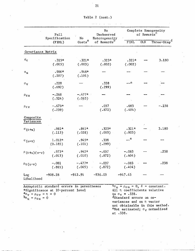
Table 2 shows the results of testing several of the restrictions

regarding heterogeneity in which we are interested. The first column

replicates the results from column (I) of 'Table L The second column

tests the restriction that all cost parameters are zero (O'v = PEV

= n

0). A likelihood ratio test indicates that the restriction is rejected

at the 90 percent level but cannot be rejected at the 95 percent level.

Thus the four cost parameters are, as a whole, barely significant. Note

that in this case the wage gain equals the welfare gain, for par-

ticipation is determined solely by the reward. Thus we can also

conclude that the difference between the welfare gain and the wage gain

in the full model is only barely significant.

In the next column we test the restriction that there is no unob-

served heterogeneity of rewards (0' = P = 0). A likelihood ratio testu EU

overwhelmingly rejects this restriction (X 2 = 56). Note too that this

restriction has a large effect on the 0 parameters. This means that

merely interacting T with other variables will not give correct

estimates. Next we further restrict the model by having no observed

heterogeneity of rewards--that is, we restrict the model to have only a

constant wage effect of participation. The OLS estimates of this model,

20

Table 2

Estimates of Restricted Models

No Complete HomogeneityFull Unobserved of Rewardsc

Specification No Heterogenei£y(FIML) . Costsa of Rewards FIML OLS Three-Stepd

Rewards (Zo)

Constant .023 .176 .626* .096 .045 1.688(.441) (.328) (.324 ) (.286) (.036) ( .353)

Age -.025* -.025* -.008( .013) (.010) ( •008)

Experience -.016 -.012 -.003(.012) (.010) (.004 )

Female -.056 -.054 .011(.127) (.117) (.036 )

Schooling -.081* -.069* -.025(.030) ( .024) (.022)

Costs(Wn)

Constant -.322 .528 .246 .160( .272) (.358) (.287)

Age .003 .002 .001(.010) (.008) (.002 ) .011

General EarningsGrowth(X/3 )

Constant 1.074* 1.016* 1. 078* 1.090* 1.107 .857( .119) (0.047) (0.133) (0.064 )

Age -.004* -.003* -.004* -.004* -.004* -.0001(.002) (.001 ) ( .002) (.002 ) ( .001) (.002 )

Experience -.005* -.004* -.005* -.005* -.005* -.005*(.002) ( .002) (.002 ) (.002) (.001) (. OOi)

Female .038* .041* .045* .044* .044* .044*(.016) (.016) (.016) (.016) (.016) (.016)

Schooling -.007* -.006* -.007* -.008* -.008* -.008*(.004) (.003 ) (.004 ) (.002 ) (.002 ) (.002)

(table continues)

---_ _._ .

21

Table. 2 (cont.)

FullSpecification

(FIML)

Covariance Matrix

NoCostsa

NoUnobserved

HeterogeneitYof Rewards

Complete Homogeneityof Rewardsc

~F-:::IM:-:'L::----;O::-=L-:::S--:T:::h-r-e-e--""O'S-t-epd

.315*(.005)

.986*(.207)

.228(.692 )

.321*(.003)

.946*(.101)

.323*(.003)

.338(.299)

.321*(.003 )

3.180

PEU

PEV

CompositeVariances

a (E+u)

a (u-v)

P (E+u) (u-v)

PE(U-V)

-.268(.524 )

-.673*(.239)

.961*( .113)

1.012*(0.185)

.973*( .013)

-.081(.865)

-.477*(.0,65)

.841*(.028 )

.945*(.101)

.942*(.010)

-.477*(.065 )

.037(.872)

.323*(.003)

.338(.299)

-.037(.872 )

-.037( .872)

.083(.404 )

.321*(.003 )

e

-.083(.404)

-.083(.404)

-.238

3.180

.238

.238

Log -908.28Likelihood

-912.91 -936.03 -947.43

Asymptotic standard errors in parentheses*Significance at 10-percent levelaav = PEV = n = 0bau = PEU = 0

ca u = PEU = 0, 0 = constant.All n coefficients relativeto av = .338.dStandard errors on co­variances and on n vectornot obtainable in this method.eNot estimated; av normalizedat .338.

22

commonly used in past studies, give low (.045) and insignificant wage

gains. The FIML estimates, which allow for self-selection via the costs,

give higher (.096) but still insig~ificant wage gains. Note too that the

estimate of the correlation across equations in this model, is low and

insignificant (.08). An analyst who has estimated this model alone might

conclude that there is no selection bias (perhaps because a first­

difference technique has been employed), but in fact that correlation is

an average of positive and negative composite correlations in the full

model (.973 and -.081, weighted toward the latter because 95.8 percent of

the sample are nonparticipants). Finally, it is interesting to compare

the FIML estimates with the results from the widely used three-step

method. The differences are again surprisingly large. Our conclusion is

that the efficiency gains of the FIML method are important in models like

ours.

c. Implications for' Wage and Welfare Gains

Using the parameter estimates from our full FIML specification, we

can calculate the expected wage and welfare gains from participating as

given in equations (14)-(15) above. The results are shown in Table 3.

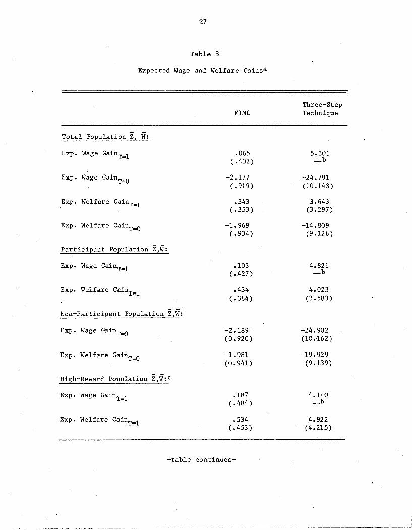
The first entry indicates that a participant with the Z and W character­

istics of the mean individual in the total population would have a wage

gain of approximately 6.5 percent. The mean wage gain of those who do

not participate is negative, as should be expected--this is part of the

reason that such individuals do not participate. The mean welfare gain

from participation is equal to about a 40 percent increase in the wage.

The welfare gain is larger than the wage gain because, in our applica­

tion, mean costs are estimated to be negative. There is nothing

23

necessary in this result, and we expect that positive costs would occur

in other applications and that therefore the welfare gain would be

smaller than the wage gain.

The standard error on the wage gain is fairly large, equal to .402.

This may seem at odds with our above results in the significance of

heterogeneity of rewards, but the two findings are quite compatible, as

illustrated in Figure 1. The mean reward in the population is -2.11, but

the fraction participating (about 5 percent) occupies only the small

upper tail of the reward distribution (the shaded region) .18 The con­

ditional mean in that tail is not far from zero, partly because the con­

ditional variance in the tail is naturally large, and partly because in

our application we have estimated negative mean costs, as already

mentioned--hence many individuals participate even though they have nega­

tive wage gains (although a few have very large wage gains).19

Nevertheless, the ~ikelihood ratio tests reported above indicate that the

wage-gain distribution as a whole is a good explainer of participation

and the wage gain from participation. A model which collapsed the

distribution on the mean would be significantly worse.

The diagram in Figure 1 also shows how our model can be used to pre­

dict the effect on earnings of changing the participant population. For

example, lowering costs--such as by paying stipends to a training program

or providing scholarships for education--would shift Wn to the left (as

shown by the arrow) .and enlarge the number of participants. Those

brought into the program obviously would have smaller wage gains than

those already in--hence the mean wage gain must fall. Mathematically,

the effect on the mean wage gain of changing costs is:

------------ ------------- -------------- ---- -------------------

24

Wage Gain(Zio+U)

20(-2.11)

Figure 1

Wn(-.21)

o .065

25

a(w.n)1

=

where the notation can be seen in the notes to Table 3. This expression

must be positive because the term in curly brackets is positive (it is

*·the expectation of (Ti/cru-v) conditional upon its being positive).

A related question with a somewhat different answer is what the

effect on mean wages in the total population would be.if costs were

lowered and participation expanded, i.e., whether economy-wide produc-

tivity would increase. Expected wage growth in the total population is:

E ( t.w. Ix. S ~ Z. 0, W1' n)

111

Hence

X.S +.Prob(T.=1)E[Z.O + u.1 T. = 1, Z.o, W.n]1 1 1 11 11

X1.S + [1 - F(s.)][Z.O + (02 /0 )f(s.)/(1 - F(s.))].

1 1 U u-v 1 1 .

aE(t.w.1 X.S, z.o, W.n)/a(w.n)1 1 1 1 1

This effect is a weighted average of rewards and costs, and hence is

ambiguous in sign. In particular, the sign can diff,er between groups

with different Z and W characteristics. In our sample, since the mean

wage gain and mean costs are both negative, the expression is positive--

hence lowering costs and increasing participation would lower mean wage

growth. This is again because negative costs imply that many par-

ticipants who are on the margin have negative wage gains. If costs were

instead positive, subsidizing them would bring in participants with

positive wage gains and hence could improve mean economy-wide wages. The

strength of our model is that these effects can be calculated explicitly.

26

The rest of the results in Table 3 are also of some interest.

Evaluating wage and welfare gains at the mean characteristics of the par­

ticipant population gives higher values of both (almost 100 percent

higher in the case of wage gains). As should be expected, those who par­

ticipate have the Z characteristics for which rewards are higher.

Likewise, as also shown in the ~able, nonparticipants have charac­

teristics for which the wage gains are more negative. A "high-reward"

population--the young, the inexperienced, and those with less schooling-­

have wage gains of almost 20 percent, almost double those of the mean

participant. Finally, the table results for the three-step technique

confirm the lack of robustness indicated in Tables 1 and 2. The wage and

welfare gains implied by the parameters are extreme and implausible.

III. SUMMARY AND CONCLUSIONS

In this paper we have extended the basic self-selection model-­

appropriate for estimating the effect on earnings of education, training,

unions, or migration--incorporate heterogeneity of rewards in returns

to the activity. We show that such heterogeneity can be neatly specified

in a model that has a close relationship to basic consumer demand theory,

and that the welfare gain to the activity can be estimated in the model.

We also demonstrate that the notion of heterogeneity of rewards has

strong implications for public policy, for it implies that bringing more

people into the activity lowers the mean rate of return. One of the

strengths of our model is that it makes these points explicit and

provides the means to calculate directly the effect of changing the cost

27

Table 3

Expected Wage and Welfare Gainsa

FIML

Total Population Z, W:

Three-StepTechnique

Exp. Wage GainT=l

Exp. Wage GainT=O

Exp. Welfare GainT=l

Exp. Welfare GainT=O

Participant Population Z,W:

Exp. Wage GainT=l

Exp. Welfare GainT=l

Non-Participant Population Z,W:

Exp. Wage GainT=O

Exp. Welfare GainT=O

High-Reward Population Z,W:c

Exp. Wage GainT=l

Exp. Welfare GainT=l

.065(.402)

-2.177(.919)

.343( .353)

-1. 969(.934)

.103( •.427 )

.434(.384)

-2.189(0.920)

-1. 981(0.941)

.187(.484 )

.534( .453)

5.306__b

-24.791(10.143)

3.643(3.297)

-14.809(9.126)

4.821__b

4.023(3.583)

-24.902(10.162)

-19.929(9.139)

4.110__b

4·922(4.215)

-table continues-

28

Notes to Table 3

aStandard errors in parentheses.

Exp. Wage GainT=l - I * --= E(Z.o + u T. > 0, Z.o, w1.n)

111

s = (W.n - z.o)/o1 1 u-v

z.o1

Variance

= Z.o - w.n + a Al1 1 u-v

Variance

Exp. Welfare GainT=O

Variance

bNegative variance.

= 02

(1 + SAl - A 2)u-v 1

CAge = 20, Experience = 2, Schooling = 9, Female = .44.

29

structure on participation probabilities and mean rewards of

participants. Our empirical application to a Swedish manpower training

program provides strong evidence of the existence of heterogeneity of

rewards.

There are several areas of additional research on this topic. First,

it would be interesting to incorporate uncertainty into the model, for

participation decisions are presumably based upon some guess about the

future returns--the actual return is not known. Another extension would

be the incorporation of involuntary nonparticipation into the model,

such as would occur if .an individual desires to be a member of a union

and cannot get a union job, or if an individual desires to enroll in an

educational or training program but cannot. 20 Finally, it would of

course be interesting to see this model applied to wage equations for

education, unions, migration, and other training programs.

30

NOTES

1Kiefer and Bassi employ a first-difference technique to eliminate

selection bias. Their stochastic model is a special case of a larger

class of panel data models that assume fixed effects. See Chamberlain

(1982) for a discus sion of such models. In this paper we will only be

concerned with the first difference technique. Note also that the

manpower-training application of Ashenfelter (1978) uses panel data.

However, selection bias is avoided in that model only if selection is

based soley upon lagged earnings, an observable variable. The more

serious problem arises when selection is affected by unobservables, the

case we are concerned with here. See Barnow, Cain, and Goldberger (1980)

for a discussion of this distinction.

2This distinction was made in an earlier paper by Moffitt (1981).

~or example, this is the model discussed by Barnow, Cain, and

Goldberger (1980) and used by Kiefer (1979) and Bassi (forthcoming).

4To put it differently: if there is no heterogeneity of costs or

preferences, and if the rate of return is constant (and positive), why do,

not all individuals participate? The common statement that bias arises'

because participation is correlated with "ability" and because "ability"

is in the linear error term 8i cannot be correct, for 8i cancels out in

the comparison of earnings with and without participation.

5Note that the equation system (10)-(13)' is observationally equiva­

lent to the general Lee (1979) model in which each regime is allowed to

have its own error term with a separate variance, and where free correla~

tion between the choice-equation error term and the two regime error

terms is allowed. Compared to that general model, which has sometimes

31

been estimated in the applied literature, our formulation only provides

an alternative interpretation of the various correlations (albeit an eco-

nomically important one). The importance of the interpretation of the

error terms can be seen by comparing our interpretation to the union

mo4el of Lee (1978). Such a comparison has been made recently by

Bjorklund (1983), who shows that in the context of our model Lee's

parameter estimates have very different implications for the magnitude of

union-wage effects than he supposed.

6Both hypotheses are nested in the full model. See notes 9 ·and 10.

7To see this, note that the earnings obtainable by participating and

by not participating in the activity respectively can be denoted

Y . + x" f3 + Z" 0 + u1" + E:" if T

1"S1 1 1 1

1

where t and s represent time periods after and before the activity.

8Note that the variance of the T* equation is identified, unlike that

of a probit equation. The reason is important. The variance is iden-

tified because the wage gain Zio appears in the T* equation with a coef-

ficient of one. This is our restriction from theory--that the partici-

pation decision must be a direct function of the dollar wage gain. T* is

thus measurable in dollar terms and its scale can be fixed. This also

relates to the identification condition on the Wand Z vectors. In the

Lee model, the same condition appears as a requirement that the coef-

ficients on Y in the selection equation be identified--the variance can-

not be identified and is normalized to one. In our model, the theo-

retical restriction we impose on those coefficients allows us to identify

32

the variance instead. This is What allows us to identify the welfare

gain in dollar terms, a crucial contribution of the paper.

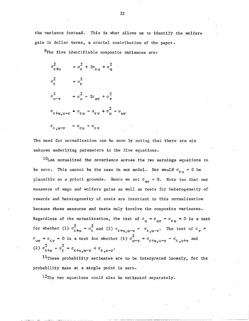
9The five identifiable composite variances are:

(j2 2 + 2(j +(j2

e+u (je EU u

'(j2 2e (je

(j2 22(j

2(j +(ju-v u uv v

(j +(j2

= (jeu (jEV - (je+u,u-v u uv

(je,u-v

(jeu

The need for normalization can be seen by noting that there are six

unknown underlying parameters in the five equations.

lOLee normalized the covariance across the two earnings equations to

be zero. This cannot be the case in our model. Nor would (jeu = 0 be

plausible on a priori grounds.' Hence we set (j = O.uv Note too that our

measures of wage and welfare gains as well as tests for heterogeneity of

rewards and heterogeneity of costs are invariant to this normalization

because these measures and tests only involve the composite variances.

Regardless of the normalization, the test of 0 = (j = (j = 0 is a' testu uv Eu

=o • The test of (je,u-v v

= 0 (j ande+u,u-v E,U+V

=(j +(je+u,u-v e u-v·. ,

= 0 0ev2 2

(j - ~e+u v e(2)

2 2for whether (1) (je+u = (je and (2) (je+u,u-v

2is a test for whether (1) (j u-v

(juv

llThese probability estimates are to be interpreted loosely, for the

probability mass at a single point is zero.

l2The two equations could also be estimated separately.

33

13The concept of fixed effect in this model is thus in relative

terms.

14In wage change equations it is common to include the change in

experi~nce and schooling on the right-hand side. In our case we find

that inappropriate because both variables are endogenous; the choice

beween participation and nonparticipation implies a choice between dif­

ferent changes in experience and schooling.

15Note that there is no identification requirement on X and Z.

16The lambda variables in these equations and those in Table 2 are

all significant at the 10 percent level.

l7Another source of imprecision in the model may lie in our not

having any variables in the selection equation that can be reasonably

excluded from the earnings equation.

18We assume v = 0 for illustration.

19Such would occur in any case, of course, since v ranges to minus

infinity. But clearly a negative mean cost results in more participants

with negative wage gains than would be the case if costs were positive.

20Such a specification would lead to a disequilibrium model of par-

ticipation (Moffitt, 1981). The bivariate probit model with partial

observability would be applicable (Poirier, 1980).

34

References

Ashenfelter, O. 1978. "Estimating the Effect of Training Programs on

Earnings." Review of Economics and Statistics (February): 47-.57.

Barnow, B., G. Cain and A. Goldberger. 1980. "Issues in the Analysis

of Selection Bias." In Evaluation Studies Review Annual, edited by

E. Stromsdorfer and G. Farkas, Vol. 5. Beverly Hills: Sage.

Bassi, L. "The Effect of CETA on the Post-Program Earnings of

Participants." Journal of Human Resources, forthcoming.

Bjorklund, A. 1983. "A Note on the Interpretation of Lee's Self­

selection Model," mimeo.

Chamberlain, G. 1982. "Panel Data." Working Paper 8209, Social Systems

Research Institute, University of Wisconsin.

Heckman, J. 1978. "Dummy Endogenous Variables in a Simultaneous

Equations System." Econometrica, ~ (July): 931-959.

1979. "Sample Selection Bias as a Specification Error."

Econometrica, !!l... (January): 153-161.

Kenny, L., L. Lee, G. Maddala. and R. Trost. 1979. "Returns to College

Education: An Investigation of Self-Selection Bias Based on Project

Talent Data." International Economic Review, lQ. (October): 775-789.

Kiefer, N. 1979. "Population Heterogeneity and Inference from Panel

Data on the Effects of Vocational Education." Journal of

Political Economy (October): S213-S226.

Lee, L. 1978. "Unionism and Wage Rates: A Simultaneous Equations Model

With Qualitative and Limited Dependent Variables." International

Economic Review, 19: 415-433.

35

Lee, 1. 1979. "Identification and Estimation in Binary Choice Models

with Limited (Censored) Dependent Variables." Econometrica,!!!...

(July): 966-977.

Maddala, G. and L. Lee. 1976. "Recursive Models Hith Qualitative

Endogenous Variables." Annals of Economic and Social Measurement,

1 (Fall): 525-544.

Mallar, C., S. Kerachsky and C. Thornton. 1980. "The Short-Term

Economic Impact of the Job Corps Program." In E. Stromsdorfer and

G. Farkas, ~. cit.

Nakasteen, R. and M. Zummei. 1980. "Migration and Income: The Question

of Self-Selection." Southern Economic Journal,~: 840-851.

Moffitt, R. 1981. "Varieties of Selection Bias in Program Evaluations."

Rutgers University, mimeo.

Nickell, S. 1982. "The Determinants of Occupational Success in

Britain." Review of Economic Studies, XLIX: 43-53.

Poirier, D. 1980. "Partial Observability in Bivariate Probit Models."

Journal of Econometrics, ~ (February): 209-217.

Vuksanovic, M. 1979. "Codebook for the Level of Living Survey 1974"

o 0

(Kodbok for 1974 ars levnadsnivaundersokning, in Swedish),

Institute for Social Research, Stockholm.

Willis, R. and S. Rosen. 1979. "Education and Self-Selection." Journal

of Political Economy (October): 87-S36.

36

Appendix A

Evaluation of the Likelihood Function

The log likelihood function is:

L = 1: log(P1 ) + E log(PO

)T=1 T=O

where

Letting f be the unit normal density function and F the cumulative normal

distribution function, the two probabilities can be factored into a con-

ditional univariate c.d.f. and a marginal univariate p.d.f.:

PI =[1 - F(r1 )] f(ZI)/cr e

Po = F(rZ) f(z3)/cr c

where

e = c + u

f u - v

(W.n - z.S)/cr,...1 1 Co

---- -~------_._--------------

r 1 (z2- Pefz1)/(1

r 2 = (z2 - Pefz3)/(1

37

Appendix A (conto)

2)1/2- Pef

2)1/2- Pef

38

Appendix B

Sample Characteristicsa

Number in the sample

Log wage aftertraining (1981)

Change in log wages,1974 to 1981.

Age (1981)

Years of schoolingbefore training (1974)

Years of work experiencebefore training (1974)

Fraction of women

Participants

87

3.502

.895

35.45

9.55

9.18

.44

NonParticipants

2014

3.561

.790

42.07

10.18

14.95

.44

a Sample includes only those with wges in both 1974 and 1980, a subset ofthe full sample.