Embed Size (px)
Citation preview

MAT 223 Linear Algebra I
University of Toronto
by Jeremy Lane(using some pieces of lecture notes by Ben Schachter)
1

Contents
1 Systems of linear equations 131.1 Linear equations . . . . . . . . . . . . . . . . . . . . . . . . . . . . 131.2 Systems of linear equations . . . . . . . . . . . . . . . . . . . . . . . 191.3 The augmented matrix of a system . . . . . . . . . . . . . . . . . . 241.4 Elementary operations . . . . . . . . . . . . . . . . . . . . . . . . . 271.5 Gaussian elimination . . . . . . . . . . . . . . . . . . . . . . . . . . 301.6 The rank of a matrix . . . . . . . . . . . . . . . . . . . . . . . . . . 331.7 Discussion: linear and nonlinear problems in science and mathematics 35
2 Matrix algebra 362.1 Equality of matrices . . . . . . . . . . . . . . . . . . . . . . . . . . 372.2 Matrix addition and scalar multiplication . . . . . . . . . . . . . . . 382.3 Matrix-vector products . . . . . . . . . . . . . . . . . . . . . . . . . 422.4 Matrix multiplication . . . . . . . . . . . . . . . . . . . . . . . . . . 452.5 Matrix transpose . . . . . . . . . . . . . . . . . . . . . . . . . . . . 492.6 Matrix equations . . . . . . . . . . . . . . . . . . . . . . . . . . . . 512.7 Discussion: non-commuting operators and quantum mechanics . . . 52
3 More systems of linear equations 533.1 The matrix equation of a system of linear equations . . . . . . . . . 533.2 Span and systems of linear equations . . . . . . . . . . . . . . . . . 553.3 Homogeneous systems of linear equations . . . . . . . . . . . . . . . 573.4 Linear combinations and basic solutions . . . . . . . . . . . . . . . 583.5 The associated homogeneous system of linear equations . . . . . . . 623.6 All roads lead to the same reduced row echelon form . . . . . . . . 63
4 Matrix inverses 664.1 Invertible matrices . . . . . . . . . . . . . . . . . . . . . . . . . . . 674.2 The inverse of a matrix . . . . . . . . . . . . . . . . . . . . . . . . . 684.3 Elementary matrices . . . . . . . . . . . . . . . . . . . . . . . . . . 714.4 The matrix inversion algorithm . . . . . . . . . . . . . . . . . . . . 73
2

4.5 The big theorem for square matrices (part 1) . . . . . . . . . . . . . 754.6 BA = I =⇒ AB = I for square matrices . . . . . . . . . . . . . . 76
5 Geometry of Rn 805.1 Review: geometry of R2 . . . . . . . . . . . . . . . . . . . . . . . . 805.2 Vectors and points . . . . . . . . . . . . . . . . . . . . . . . . . . . 845.3 Addition, scalar multiplication, and lines . . . . . . . . . . . . . . . 865.4 The distance between two points . . . . . . . . . . . . . . . . . . . 895.5 The dot product . . . . . . . . . . . . . . . . . . . . . . . . . . . . 915.6 The angle between two vectors . . . . . . . . . . . . . . . . . . . . . 935.7 Orthogonal projection . . . . . . . . . . . . . . . . . . . . . . . . . 945.8 Planes in R3 . . . . . . . . . . . . . . . . . . . . . . . . . . . . . . . 965.9 Hyperplanes in Rn . . . . . . . . . . . . . . . . . . . . . . . . . . . 1005.10 Application: binary classifiers in R2 . . . . . . . . . . . . . . . . . . 1015.11 Discussion: geometry of the universe . . . . . . . . . . . . . . . . . 102
6 Linear transformations 1046.1 Functions from Rn to Rm . . . . . . . . . . . . . . . . . . . . . . . . 1046.2 Linear transformations . . . . . . . . . . . . . . . . . . . . . . . . . 1066.3 Matrix transformations are linear . . . . . . . . . . . . . . . . . . . 1076.4 Transformations of R2 . . . . . . . . . . . . . . . . . . . . . . . . . 1086.5 The matrix of a linear transformation . . . . . . . . . . . . . . . . . 1116.6 Example: orthogonal projection onto a line . . . . . . . . . . . . . . 1126.7 Composition of linear transformations . . . . . . . . . . . . . . . . . 1146.8 Kernel and image . . . . . . . . . . . . . . . . . . . . . . . . . . . . 1156.9 Invertible linear transformations . . . . . . . . . . . . . . . . . . . . 1196.10 Discussion: solving nonlinear problems by linear approximation . . 122
7 Subspaces, span, and linear independence 1247.1 Subspaces . . . . . . . . . . . . . . . . . . . . . . . . . . . . . . . . 1247.2 The span of a set of vectors . . . . . . . . . . . . . . . . . . . . . . 1287.3 Linear independence . . . . . . . . . . . . . . . . . . . . . . . . . . 1317.4 Basis . . . . . . . . . . . . . . . . . . . . . . . . . . . . . . . . . . . 1357.5 Dimension . . . . . . . . . . . . . . . . . . . . . . . . . . . . . . . . 1387.6 Discussion: . . . . . . . . . . . . . . . . . . . . . . . . . . . . . . . 139
8 The fundamental subspaces of a matrix 1418.1 The null space of a matrix . . . . . . . . . . . . . . . . . . . . . . . 1418.2 The column space of a matrix . . . . . . . . . . . . . . . . . . . . . 1458.3 The row space of a matrix . . . . . . . . . . . . . . . . . . . . . . . 1478.4 Row and column spaces . . . . . . . . . . . . . . . . . . . . . . . . 149
3
8.5 Big theorems . . . . . . . . . . . . . . . . . . . . . . . . . . . . . . 150
9 Determinants 1549.1 Definition of the determinant . . . . . . . . . . . . . . . . . . . . . 1549.2 Properties of the determinant . . . . . . . . . . . . . . . . . . . . . 1599.3 Determinants and area . . . . . . . . . . . . . . . . . . . . . . . . . 1629.4 Application: multivariable integration and the determinant of the
Jacobian . . . . . . . . . . . . . . . . . . . . . . . . . . . . . . . . . 163
10 Eigenvalues and eigenvectors 16510.1 Eigenvalues and Eigenvectors . . . . . . . . . . . . . . . . . . . . . 16510.2 Computing eigenvalues and eigenvectors . . . . . . . . . . . . . . . 16610.3 Eigenspaces . . . . . . . . . . . . . . . . . . . . . . . . . . . . . . . 16810.4 Algebraic multiplicity of eigenvalues . . . . . . . . . . . . . . . . . . 17010.5 Diagonalization . . . . . . . . . . . . . . . . . . . . . . . . . . . . . 17110.6 Application: google page rank . . . . . . . . . . . . . . . . . . . . . 17710.7 Application: eigenvalues and eigenvectors in classical and quantum
mechanics . . . . . . . . . . . . . . . . . . . . . . . . . . . . . . . . 177
11 Orthogonality 17911.1 Orthogonality . . . . . . . . . . . . . . . . . . . . . . . . . . . . . . 17911.2 Orthogonal complements . . . . . . . . . . . . . . . . . . . . . . . . 18311.3 Orthogonal projection onto a subspace . . . . . . . . . . . . . . . . 18811.4 The Gram-Schmidt algorithm . . . . . . . . . . . . . . . . . . . . . 19111.5 Application: QR factorization and linear regression . . . . . . . . . 193
12 Singular Value Decomposition 19512.1 Singular Value Decomposition . . . . . . . . . . . . . . . . . . . . . 19512.2 Application: principal component analysis . . . . . . . . . . . . . . 195
A Extra examples for Chapter 1 196
B Tutorials 201B.1 Tutorial 1: solving systems of linear equations . . . . . . . . . . . . 201B.2 Tutorial 2: matrix algebra . . . . . . . . . . . . . . . . . . . . . . . 203B.3 Tutorial 3: More systems of linear equations . . . . . . . . . . . . . 208B.4 Tutorial 4: Matrix inverses . . . . . . . . . . . . . . . . . . . . . . . 210B.5 Tutorial 5: Vector geometry . . . . . . . . . . . . . . . . . . . . . . 213B.6 Tutorial 6: Linear transformations . . . . . . . . . . . . . . . . . . . 216B.7 Tutorial 7: Subspaces, spanning, and linear independence . . . . . 220B.8 Tutorial 8: The fundamental subspaces of a matrix . . . . . . . . . 222B.9 Tutorial 9: Determinants . . . . . . . . . . . . . . . . . . . . . . . . 227
4

B.10 Tutorial 10: Eigenvalues, eigenevectors, and diagonalization . . . . 230B.11 Tutorial 11: Orthogonality . . . . . . . . . . . . . . . . . . . . . . . 232
C Tutorial sample solutions 235C.1 Tutorial 1-4 . . . . . . . . . . . . . . . . . . . . . . . . . . . . . . . 235C.2 Tutorial 5-8 . . . . . . . . . . . . . . . . . . . . . . . . . . . . . . . 249C.3 Tutorial 9-11 . . . . . . . . . . . . . . . . . . . . . . . . . . . . . . 275
5

About these notes
These lecture notes were created for the course MAT 223 at the Universityof Toronto, Summer of 2017, by Jeremy Lane. They are partially based on theprevious Summer’s course which used selected chapters from Linear algebra withapplications by Keith Nicholson. Pieces of these notes are taken or adapted froma previous set of lecture notes for linear algebra, written and graciously shared byBen Schachter. In particular, all .tikz diagrams were created by Ben. All mistakesare mine, not Ben’s.
These lecture notes are designed to be lecture notes and as such it may be dif-ficult to use them for independent learning. They feature many in-class exercisesand tutorial questions which ask the students to reach conclusions on their own,with the aid of the instructors and teaching assistants. Various constructions, al-gorithms, proofs, and definitions are not spelled out explicitly in the notes, butrather indicated by examples and exercises. Many blanks will be filled in in thelectures. This will benefit students who attend and participate in all of the lecturesand tutorials. Students should attempt to write full, detailed answers to all of thein-class exercises and tutorials as writing is one of the most effective ways to learnmath.
The main textbook for this instance of the course is Linear algebra and itsapplications by Lay. Lay makes several pedagogical choices about the order inwhich he introduces key concepts. These notes eschew some of those choices andopt for a more straightforward development of the theory. In particular, we leavethe introduction of linear transformations, span, and linear independence to theirown chapters instead of piling them all into the first chapter.
Please email me with any typographical or factual errors you find in thesenotes: [email protected].
On the front page: Ferns have astonishing self-similarities. The Barnsley Fern is afractal that resembles a fern and can be created using affine transformations. Seethe webpage https://en.wikipedia.org/wiki/Barnsley_fern. This particularphoto belongs to the author.
Copyright: Until I have time to read the details of various open source licences,you may consider these lecture notes as free and open in whatever sense you deemreasonable (in particular, you can have the .tex source if you like).
6

Pedagogical remarks
• The only prerequisite for MAT 223 is high school calculus (and by extension,some high school level geometry and trigonometry). Although some studentsin the course have much more background, these notes are written withthe prerequisite in mind and start from scratch. In particular, the notesbegin with the assumption that the students’ knowledge of mathematicalterminology, conventions, etc. is very limited or has been forgotten overtime. The first few chapters are designed as if the students are being taughta language, not just math (indeed, the format was partially inspired by takingclasses at Alliance Francaise).
• The earlier chapters of the notes attempt to make a strong “backwards”connection between the concepts and terminology that are being introducedand things that should already be familiar with the students (such as highschool algebra and geometry of the xy-plane). This is repeated in Chapter5, which begins with a rough summary of high school geometry the studentsare expected to know (which is then generalized to Rn).
• In Chapter 1, we define the rank of a matrix as the number of leading entriesin a reduced echelon form (a proof is given at the end of Chapter 3). Thisallows us to begin working with rank as a number early in the course, beforelater using it in the rank-nullity theorem. At some points we reference therank of the coefficient matrix A of a system of linear equations AND therank of the augmented matrix [A|b] (it’s a matrix so it has a rank).
• The first four chapters are very algebraic (except a few examples that areillustrated in the xy-plane). This may seem a bit dry, but – in my opinion –forcing the students to work purely algebraically with the definitions beforeintroducing any “geometric intuition” is key when many students do nothave an experience with abstraction or proofs. Pictures are pretty but canbe very confusing and discourage adopting a rigorous mentality.
Starting in Chapter 2, we emphasize how powerful properties of matrix al-gebra are by presenting many algebraic proofs (starting with an expressionand manipulating it using properties of matrix algebra until we reach an-other desired expression). The skill of doing these abstract “calculations” isa main learning goal for the course.
• Throughout, we use ‘=’ to mean that two expressions are equal, and ‘:=’ tomean the assignment operator, i.e. this is equal to that by definition.
7
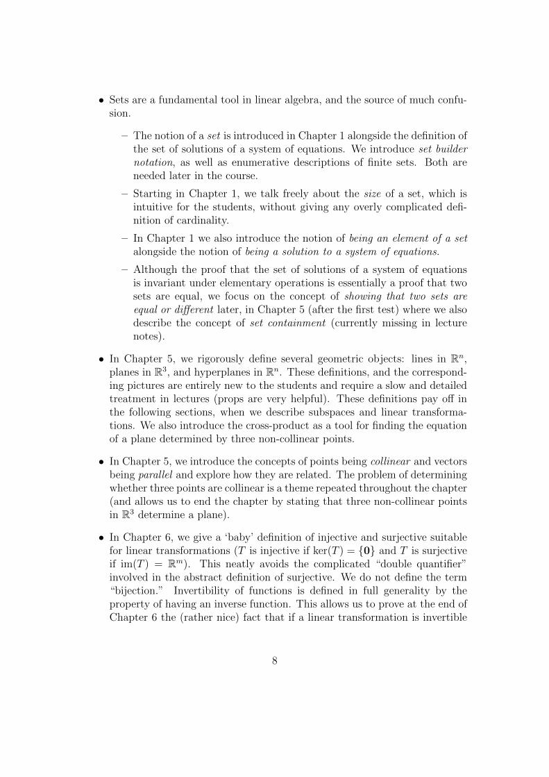
• Sets are a fundamental tool in linear algebra, and the source of much confu-sion.
– The notion of a set is introduced in Chapter 1 alongside the definition ofthe set of solutions of a system of equations. We introduce set buildernotation, as well as enumerative descriptions of finite sets. Both areneeded later in the course.
– Starting in Chapter 1, we talk freely about the size of a set, which isintuitive for the students, without giving any overly complicated defi-nition of cardinality.
– In Chapter 1 we also introduce the notion of being an element of a setalongside the notion of being a solution to a system of equations.
– Although the proof that the set of solutions of a system of equationsis invariant under elementary operations is essentially a proof that twosets are equal, we focus on the concept of showing that two sets areequal or different later, in Chapter 5 (after the first test) where we alsodescribe the concept of set containment (currently missing in lecturenotes).
• In Chapter 5, we rigorously define several geometric objects: lines in Rn,planes in R3, and hyperplanes in Rn. These definitions, and the correspond-ing pictures are entirely new to the students and require a slow and detailedtreatment in lectures (props are very helpful). These definitions pay off inthe following sections, when we describe subspaces and linear transforma-tions. We also introduce the cross-product as a tool for finding the equationof a plane determined by three non-collinear points.
• In Chapter 5, we introduce the concepts of points being collinear and vectorsbeing parallel and explore how they are related. The problem of determiningwhether three points are collinear is a theme repeated throughout the chapter(and allows us to end the chapter by stating that three non-collinear pointsin R3 determine a plane).
• In Chapter 6, we give a ‘baby’ definition of injective and surjective suitablefor linear transformations (T is injective if ker(T ) = {0} and T is surjectiveif im(T ) = Rm). This neatly avoids the complicated “double quantifier”involved in the abstract definition of surjective. We do not define the term“bijection.” Invertibility of functions is defined in full generality by theproperty of having an inverse function. This allows us to prove at the end ofChapter 6 the (rather nice) fact that if a linear transformation is invertible
8
as a function, then the inverse function must also be linear.
We use the terms ‘domain’, ‘codomain’, and ‘image’. We avoid use of theword ‘range’ because some people use it to mean ‘codomain’ and some use itto mean ‘image’, and we have no interest in participating in this confusion.
• Throughout the lectures, there are two types of interactive features. Unfor-tunately, these features grow thinner towards the end of the lecture notesdue to the time constraints involved in creating detailed notes.
– “Check your understanding” boxes typically follow a new definition orpiece of terminology. In class, students are given 1-2 minutes to writedown their answers, then a full answer is provided by the instructor onthe blackboard. Following the answer, there is a pause for questions(ideally, at this point students who did not understand some simpleaspect of the new definition will realize they are confused and ask aquestion).
– “In-class exercises” are longer problems that require the students to doa longer computation (they are given 5-10 minutes for these problems).Some of these questions have subtle complications built into them, inorder to generate discussion. After this time, a full solution was pre-sented on the board by the instructor.
Both of these features are designed to prompt interaction from students bygiving them opportunities to solve problems and ask questions, as opposedto demanding that they participate. In my experience, demanding studentparticipation causes anxiety and actually decreases participation.
Note: These lecture notes need more worked examples, but examples take a longtime to write and my time was limited. Many examples were added in lecture.
Also note: The quality of the notes decreases towards the end of the course (dueto time constraints).
9

Topics not covered in these lecture notes: There are many things oftencontained in a first course in linear algebra that we did not cover. Here are someof those things.
• Cramer’s rule.
• The adjugate formula for the inverse of a matrix.
• The interpretation of diagonalization as a ‘change of basis’.
• The notation for writing the ‘coordinates’ of a vector in a fixed basis.
• Similarity of matrices (we only covered diagonalization).
• The spectral theorem.
• Complex eigenvalues.
• The general definition of inner products.
• The axioms of a vector space (everything is Rn and subspaces of Rn).
• Jordan normal form.
10

How to use these notes alongside Lay-Lay-McDonald
The chapters of this document correspond loosely in content to the follow-ing sections in Linear algebra and its applications, fifth edition by Lay, Lay, andMcDonald.
Ch 1. Systems of linear equations See sections
• 1.1, 1.2
Ch 2. Matrix algebra See sections
• 1.3 (vector equations), 1.4 (matrix equations),
• 2.1 (matrix operations)
Ch 3. More systems of linear equations See sections
• 1.3 (linear combinations), 1.4
• 1.5 (homogeneous systems and particular solutions)
Ch 4. Matrix inverses See sections
• 2.2 (definition, properties, elementary matrices, algorithm for finding in-verses), 2.3 (the big theorem for square matrices)
Test 1: Sections 1.1-1.5, 2.1-2.3.
Ch 5. Vector geometry See sections
• 1.3, parts of 6.1 (dot product, length, orthogonality). Lay does not go intomuch detail on geometry until later chapters that are more sophisticated.The lecture notes are a good reference for this material. The textbook byNicholson is also very good.
Ch 6. Linear transformations See sections
• 1.8 Linear transformations
• 1.9 The matrix of a linear transformation
Ch 7. Subspaces, spanning, and linear independence See sections
• 1.3 (span), 1.7 (linear independence)
• 2.8, 2.9
Ch 8. The fundamental subspaces of a matrix See sections
• 2.8, 2.9
11

Test 2: Sections 1.7-1.9, 2.8-2.9, 6.1.
Ch 9. Determinants See sections
• 3.1, 3.2, and parts of 3.3
Ch 10. Eigenvalues and eigenvectors See sections
• 5.1-5.3
Ch 11. Orthogonality See sections
• 6.1-6.4
Final exam: In addition to the material from Test 1 and Test 2, the final examcovers material from sections 3.1, 3.2, and parts of 3.3, 5.1-5.4, and 6.1-6.4.
12

Chapter 1
Systems of linear equations
Before beginning this section, it may be helpful to review the followingterminology from high school algebra:
• expression
• polynomial
• term of a polynomial
• equation
• coefficient of a term
• variable
• solution of an equation
1.1 Linear equations
You are already familiar with equations involving variables from highschool. Forexample, the Pythagorean Theorem is the equation
a2 + b2 = c2
where a, b, and c are variables that represent the lengths of the sides of a right-triangle (and c is the length of the hypotenuse). For instance, if we take theright-triangle whose shorter side lengths are a = 3 and b = 4, then this equationtells us that the length of the hypotenuse must be 5.
13

Another equation you are familiar with is the equation of a line,
y = mx+ b
where x and y are variables that represent the xy-coordinates of a point in thexy-plane, and m and b are fixed numbers: m is the slope of the line, and b is they-intercept. For instance, the equation
y = 2x+ 1
describes a line in the xy-plane whose slope is 2 and whose y-intercept is 1. Thepoints on this line are precisely the points whose xy-coordinates (x0, y0) solve thisequation.
The study of linear equations is concerned with equations similar to the secondexample (the equation of a line in the xy-plane). However, we do not want torestrict ourselves to only two variables x and y, we want to be able to work withas many variables as we want or need (2, 3, 18, 56, and so on). In general, wedefine a linear equation in n variables, where n is whatever positive integer wewant, the following way.
Definition 1.1. A linear equation in n variables is an equation of the form
a1x1 + a2x2 + · · ·+ anxn = b
where a1, a2, . . . , an, b are fixed numbers and x1, x2, . . . , xn are variables. Thenumbers a1, a2, . . . , an that multiply the variables are called coefficients of theequation and the number b is called the constant term of the equation.
Remark 1.2. The word linear derives from the latin word for “a line” and means“resembling a line, of or pertaining to a line.” We call these equations linear, sincethey resemble the equation of a line in the xy-plane.
When we have many variables, we often use letters numbered with subscripts,such as x1, . . . , xn or y1, . . . , yn for our variables. When there are only one, two,or three variables, it is common to use letters such as x, y, z or u, v, w for variables.
Example 1.3. The equation2x+ 3y = 6
is linear. The variables are x and y. The coefficients are 2 and 3. The constantterm is 6.
14

Example 1.4. The equation
x2 + 2xy + y2 = 1
is not linear in the variables x and y.
Example 1.5. The equation
4 + 4z1 = 6z2 − πz3 − 10 + 8z4
is linear, even though it is not written precisely the same way as in Definition1.1. The variables are z1, z2, z3, z4. We can rearrange this equation so that it looksmore like the equation in Definition 1.1:
4z1 − 6z2 + πz3 − 8z4 = −6.
What are the coefficients of this equation? What is the constant term?
Example 1.6. Most equations that we encounter in math are not linear. For ex-ample, the following equations are not linear in the variables x and y:
y = x2, y = ex, xy = 1.
Check your understanding
Einstein’s famous “mass-energy equivalence” equation says that
E = mc2
where E is total energy of an object, m is mass of the object, and c is thespeed of light.
Is Einstein’s equation linear?
Hint: what are the variables and constants in this equation?
R2 is the set of all pairs (s1, s2) of real numbers s1 and s2. Geometrically,every pair of numbers (s1, s2) in R2 corresponds to a point in the xy-plane withcoordinates x = s1 and y = s2.
Solutions of the equationy = 2x+ 1
15

are pairs of numbers (s1, s2) ∈ R2 such that x = s1 and y = s2 solves the equation,i.e. such that
s2 = 2s1 + 1.
The set of all solutions (s1, s2) of this equation corresponds to the set of points onthe line in the xy-plane with slope 2 and y-intercept 1. We can also describe theset of solutions using set-builder notation,{
(x, y) ∈ R2 : y = 2x+ 1}.
Set-builder notation:
A set is a collection of objects. Examples of sets include the set of allsocks in my closet, the set of all apartments in Toronto, and the set of all realnumbers.
We describe sets using set-builder notation, which is as follows. The nota-tion
{x : P (x)}
which will be read as “the set of all objects x which satisfy condition P” or“the set of all objects x for which property P is true.” If it is important tospecify that the objects in a all lie in some particular domain, sometimes thefollowing notation will be used:
{x ∈ Domain : P (x)}.
This is read as “the set of all x in Domain for which property P is true.”The symbol ∈ means “is an element of.” Some examples include
• {x ∈ R : x > 0} is the set of all x in the set of real numbers for which xis strictly greater than zero. 1 is an element of this set since 1 > 0. −1is not an element of this set. Is 0 and element of this set?
• {s ∈ my shirts : s is blue} is the set of all shirts in my closet that areblue. My white shirts are not elements of this set. Similarly, my socksare not an element of this set. On the other hand, my Blue Jays shirt isan element of this set because it is blue.
16

Since the set-builder notation describing a set is often lengthy, we often use aletter or symbol to represent a set. For instance, we might call
B := {s ∈ my shirts : s is blue}.
With this notation, we could describe the fact that my Blue Jays shirt is blueby writing
my Blue Jays shirt ∈ B.
In plain english, this sentence reads, “my Blue Jays shirt is an element of theset of my shirts which are blue.”
We will learn more about set-builder notation and sets throughout thiscourse.
More generally, we call a list of real numbers (s1, . . . , sn) a n-tuple of real num-bers1, and denote by Rn (pronounced “r-n”) the set of all n-tuples of real numbers.For the time being, we will focus on the algebraic aspects of solutions to linearequations.
Definition 1.7. A solution of a linear equation
a1x1 + a2x2 + · · ·+ anxn = b
is a n-tuple (s1, . . . , sn) of real numbers such that
a1s1 + a2s2 + . . .+ ansn = b.
In other words, when we let x1 = s1, x2 = s2, . . . xn = sn, the equation is true.
Example 1.8. The pair of numbers (3, 0) is a solution of the equation
2x+ 3y = 6.
On the other hand, the pair of numbers (3, 1) is not a solution of the equation.We write
(3, 1) 6∈{
(x, y) ∈ R2 : 2x+ 3y = 6}
which reads “The pair (3, 1) is not an element of the set of pairs (x, y) of realnumbers which solve the equation 2x + 3y = 6.” More succinctly, we can simplysay “The pair (3, 1) is not a solution of the equation 2x+ 3y = 6.”
1A 2-tuple is just another name for a pair of numbers, (x, y).
17

Check your understanding
Which of the following 4-tuples are solutions of the linear equation in Ex-ample 1.5?
(0, 0, 0, 0), (1,−1, 1,−1), (2, 0, 0, 1)
Try to express your answer using set-builder notation and the symbols ∈and 6∈.
In mathematics, a common goal when given an equation is to describe ALL itssolutions. For example, for the equation
x2 = 1,
we are not content with the answer x = 1 because there is another solution,x = −1. The set of solutions to this equation could be described in set-buildernotation as
{x ∈ R : x2 = 1}.We know that this set contains exactly two numbers, 1 and −1. In this case, it ismore simple to describe this set by listing its elements:
{1,−1}
Enumerative descriptions of sets: There are various ways to describesets. We have already seen set-builder notation. In the preceding example, wesaw that we could express the set {x ∈ R : x2 = 1} by simply writing {1,−1}.
What have we done here? When we write {1,−1} we simply mean “theset consisting of the elements 1 and −1.” We simply list the elements of theset and add curly braces to indicate that we are describing a set.
This is a common way to describe sets that are small such as the one inthe example above. In general, a description of a set given in this manner – bylisting its elements inside curly braces – is called an enumerative description.The name is not particularly important.
As we will see later on, the fact that one set can be described severaldifferent ways will lead to some challenging problems. In the example above,we explained why the set-builder notation
{x ∈ R : x2 = 1}
and the enumerative description {1,−1} are actually describing the same set.We will return to this concept many times throughout the course.
18

1.2 Systems of linear equations
A system of equations is a list of several equations. For example, one can have asystem of equations that includes some non-linear equations, such as
x2 + y2 = 1, x = y
or one can have a system of equations that only includes linear equations, such as
y = 2x+ 1, x = y + 2.
In this class we are mainly interested in the second kind of system.
Since mathematicians are greedy, we would like to be able to consider systemswith as many equations as we want and as many variables as we want.
Definition 1.9. A system of m linear equations in n variables is a list of m linearequations of the form
m equations
a11x1 + a12x2 + · · · + a1nxn = b1a21x1 + a22x2 + · · · + a2nxn = b2
...am1x1 + am2x2 + · · · + amnxn = bm
where x1, . . . , xn are variables, aij are coefficients, and bi are constant terms.
An n-tuple (s1, . . . , sn) of numbers is a solution of this system of equations ifit is a solution of every equation in the system.
Notation: In the definition above, we write aij and bi. What does this mean?
• There are m equations, and we label the equations 1, 2, 3, . . . up to m.In equation 1, we call the constant term b1. In equation 2 we call theconstant term b2, and so on. If i is an integer between 1 and m, then
we write bi to mean the constant term of equation i.
19

• There are also n variables, which we have already labelled x1, x2, . . . andso on, up to xn. If 1 ≤ i ≤ m , and 1 ≤ j ≤ n, then
we write aij to mean the coefficient of xj in equation i.
•
a11x1 + a12x2 = b1
a21x1 + a22x2 = b2
Case a: Different slopesThe intersection is the unique solution (in red).
a21x1 + a22x2 = b2
a11x1 + a12x2 = b1
Case b: Same slopes, non-intersectingThere are no solutions.
a11x1 + a12x2 = b1
a21x1 + a22x2 = b2
Case c: Same slopes, coincidingThere are infintely many solutions (in red).
Example 1.10 (Systems of two linear equations in two variables). Since each linearequation in two variables describes a line in the xy-plane, solutions of a system oflinear equations in two variables can be interpreted geometrically as intersectionsof lines in the xy-plane. For example,
a) The equations in the system
y = x
y = 2x+ 3
20

describe two lines with different slopes which necessarily intersect at one point.
b) The equations in the system
y = x+ 4
y = x− 4
describe two parallel lines with different y-intercepts. Since parallel lines donot intersect, the system has zero solutions.
c) Both equations in the system
y = x+ 1
2y = 2x+ 2
describe the same line. Thus, every point on this line is a solution of the systemof linear equations. Since there are infinitely many points on a line, the systemhas infinitely many solutions.
Example 1.11. Consider the system of two equations in the variables x, y, z,
x + 2y − z = 02x + y + z = 2
We would like to describe all solutions of this system. In other words, we want tofind all 3-tuples (s1, s2, s3) that solve both equations.
If we add the two equations together, the z terms cancel and leave us with
3x+ 3y = 2
which simplifies to
x =2
3− y.
Substituting this equation back into the first equation in the system, we get(2
3− y)
+ 2y − z = 0
which simplifies to
y = z − 2
3.
21

Thus, every solution to this system is of the form(4
3− z, z − 2
3, z
).
On the other hand, for every real number t, we can check that(4
3− t, t− 2
3, t
)is a solution to the system of linear equations. We do this by plugging x = 4
3− t,
y = t− 23
and z = t into the original equations and checking that(4
3− t)
+ 2
(t− 2
3
)− t = 0
and
2
(4
3− t)
+
(t− 2
3
)+ t == 2.
Thus we have shown that the set of all solutions of the system of linear equationsis the set of all 3-tuples (
4
3− t, t− 2
3, t
),
where t is any real number. We can express the set of all such 3-tuples in setbuilder notation like this:{(
4
3− t, t− 2
3, t
)∈ R3 : t ∈ R
}Another way to describe the set of solutions is by writing
x =4
3− t
y = t− 2
3z = t
where t is any real number. We call t a parameter of the set of solutions.
Example 1.10.b) also demonstrates the following. It is possible for a system oflinear equations to have no solutions. We call a system with no solutions “incon-sistent.”
22
Definition 1.12. A system of linear equations is called consistent if it has solu-tions, otherwise it is called inconsistent.
Example 1.10 also demonstrates that, if a system of linear equations is consis-tent, then it is possible that it can have exactly one solution or infinitely manysolutions. In fact, these are the only two possibilities! This is our first theorem oflinear algebra.
Theorem 1.13. If a system of linear equations has more than one solution, thenit has infinitely many solutions.
Proof. Suppose we are given an arbitrary system of m linear equations in n vari-ables, which we can write as
a11x1 + a12x2 + · · · + a1nxn = b1a21x1 + a22x2 + · · · + a2nxn = b2
...am1x1 + am2x2 + · · · + amnxn = bm
In order to prove the theorem, we must show that:
If this system has more than one solution, then it has infinitely many solutions.
This is left as an important exercise. See Part 3 of Tutorial B.1.
To summarize, for a system of linear equations there are only three possiblecases:
(a) The system has no solutions (inconsistent).
(b) The system has solutions (consistent). There are two possibilities:
(i) The system has exactly one solution.
(ii) The system has infinitely many solutions.
Check your understanding
The equationx2 = 1
has exactly two solutions. Does this contradict Theorem 1.13?
23
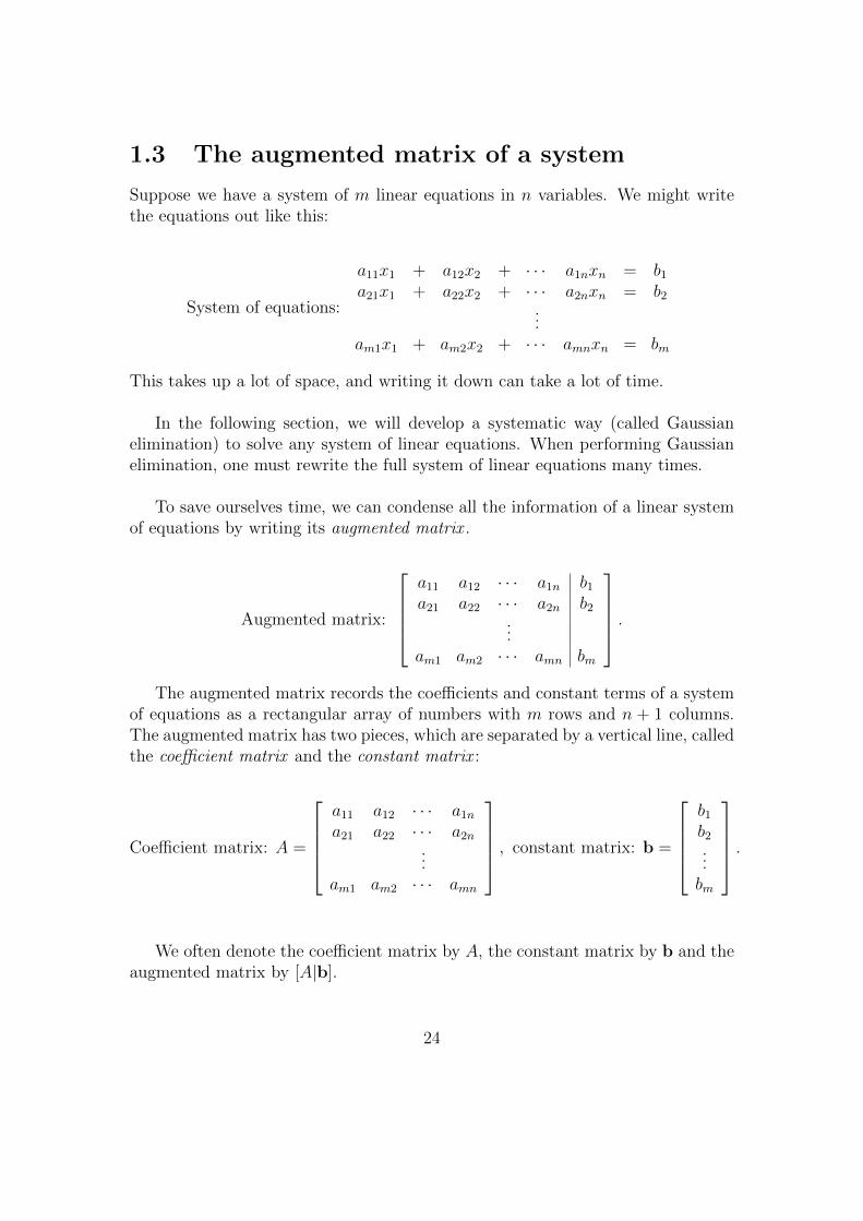
1.3 The augmented matrix of a system
Suppose we have a system of m linear equations in n variables. We might writethe equations out like this:
System of equations:
a11x1 + a12x2 + · · · a1nxn = b1a21x1 + a22x2 + · · · a2nxn = b2
...am1x1 + am2x2 + · · · amnxn = bm
This takes up a lot of space, and writing it down can take a lot of time.
In the following section, we will develop a systematic way (called Gaussianelimination) to solve any system of linear equations. When performing Gaussianelimination, one must rewrite the full system of linear equations many times.
To save ourselves time, we can condense all the information of a linear systemof equations by writing its augmented matrix .
Augmented matrix:
a11 a12 · · · a1n b1a21 a22 · · · a2n b2
...am1 am2 · · · amn bm
.The augmented matrix records the coefficients and constant terms of a system
of equations as a rectangular array of numbers with m rows and n + 1 columns.The augmented matrix has two pieces, which are separated by a vertical line, calledthe coefficient matrix and the constant matrix :
Coefficient matrix: A =
a11 a12 · · · a1na21 a22 · · · a2n
...am1 am2 · · · amn
, constant matrix: b =
b1b2...bm
.
We often denote the coefficient matrix by A, the constant matrix by b and theaugmented matrix by [A|b].
24
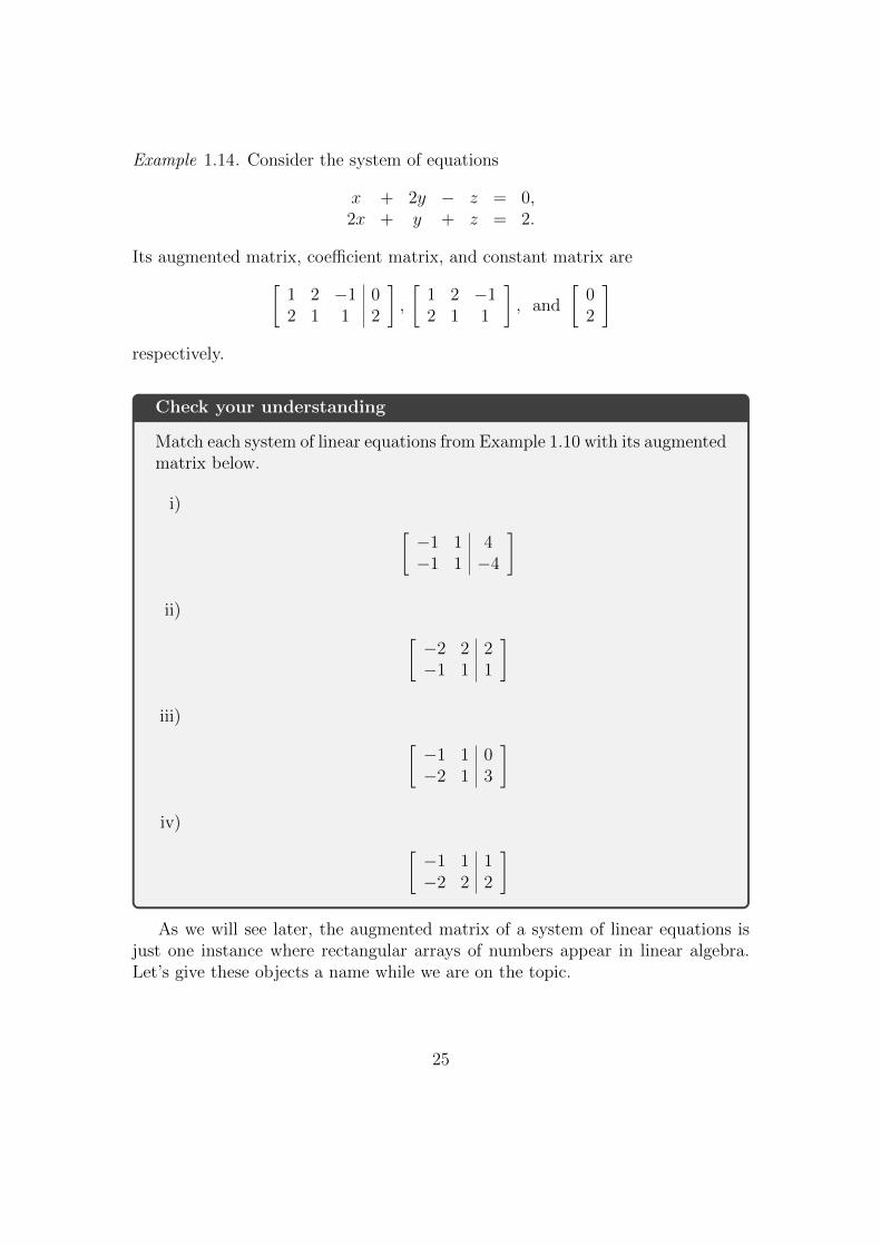
Example 1.14. Consider the system of equations
x + 2y − z = 0,2x + y + z = 2.
Its augmented matrix, coefficient matrix, and constant matrix are[1 2 −1 02 1 1 2
],
[1 2 −12 1 1
], and
[02
]respectively.
Check your understanding
Match each system of linear equations from Example 1.10 with its augmentedmatrix below.
i) [−1 1 4−1 1 −4
]ii) [
−2 2 2−1 1 1
]iii) [
−1 1 0−2 1 3
]iv) [
−1 1 1−2 2 2
]As we will see later, the augmented matrix of a system of linear equations is
just one instance where rectangular arrays of numbers appear in linear algebra.Let’s give these objects a name while we are on the topic.
25

Definition 1.15. A m×n matrix 2 is a rectangular array of numbers and/or vari-ables that has m rows and n columns.
The rows and columns of a matrix are always numbered the same way: therows are numbered in increasing order from top to bottom, the columns are num-bered in increasing order from left to right.
The i, j entry (or ijth entry) of a matrix is the number that is in the ith rowand the jth column.
Example 1.16. (a) A matrix with the same number of rows and columns is calleda square matrix . For instance, the 3× 3 matrix 1 0 0
1 0 10 −1 1
is a square matrix. The 2, 3 entry of this matrix is 1 whereas the 3, 2 entryis −1. The 1st row of the matrix is [1 0 0] whereas the 3rd row is [0 − 1 1].What is the 2nd column?
(b) A matrix with only one column is called a column vector . For instance, the4× 1 matrix
−21167
is a column vector. The 3, 1 entry is 6.
(c) A matrix with only one row is called a row vector . For instance, the 1 × 4matrix [
−2 11 6 7]
is a row vector. The 1, 3 entry is 6.
2The plural of matrix is matrices.
26

In-class exercise
If the augmented matrix of a system of linear equations contains a row ofthe form
[0 · · · 0 1],
what can be said about the set of solutions of the system of linear equations?
Warning
The augmented matrix of a system of m linear equations in n variables isNOT a m× n matrix!
a11 a12 · · · a1n b1a21 a22 · · · a2n b2
...am1 am2 · · · amn bm
.It is a m× (n+ 1) matrix, since there are n columns of coefficients, and onecolumn of constants. The coefficient matrix is a m× n matrix.
Unlike augmented matrices of systems of equations, most matrices don’thave a line drawn through them. The vertical line in an augmented matrixis just decoration.
1.4 Elementary operations
In order to describe a uniform approach to solving systems of linear equations, wefirst describe three ways to manipulate a system of equations called elementaryoperations.
The three elementary operations on a system of linear equations are:
I) Interchanging two equations,
II) Multiplying an equation by a non-zero number, and
III) Adding a multiple of one equation to another equation.
27
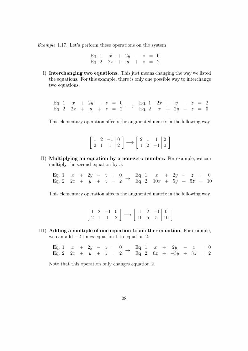
Example 1.17. Let’s perform these operations on the system
Eq. 1 x + 2y − z = 0Eq. 2 2x + y + z = 2
I) Interchanging two equations. This just means changing the way we listedthe equations. For this example, there is only one possible way to interchangetwo equations:
Eq. 1 x + 2y − z = 0Eq. 2 2x + y + z = 2
−→ Eq. 1 2x + y + z = 2Eq. 2 x + 2y − z = 0
This elementary operation affects the augmented matrix in the following way.
[1 2 −1 02 1 1 2
]−→
[2 1 1 21 2 −1 0
]II) Multiplying an equation by a non-zero number. For example, we can
multiply the second equation by 5.
Eq. 1 x + 2y − z = 0Eq. 2 2x + y + z = 2
→ Eq. 1 x + 2y − z = 0Eq. 2 10x + 5y + 5z = 10
This elementary operation affects the augmented matrix in the following way.
[1 2 −1 02 1 1 2
]−→
[1 2 −1 010 5 5 10
]III) Adding a multiple of one equation to another equation. For example,
we can add −2 times equation 1 to equation 2.
Eq. 1 x + 2y − z = 0Eq. 2 2x + y + z = 2
→ Eq. 1 x + 2y − z = 0Eq. 2 0x + −3y + 3z = 2
Note that this operation only changes equation 2.
28

Check your understanding
How does the augmented matrix change when you add −2 times equation 1to equation 2 in the previous example?
Every elementary operation can be reversed by another elementary operation.
Check your understanding
For each elementary operation in the example above, describe the opposite(or inverse) elementary operation.
As we saw in the previous example, for each elementary operation on a systemof linear equations, there is a corresponding operation on the rows of the aug-mented matrix. We call these elementary row operations.
In-class exercise
List the three types of elementary row operations on a matrix.
Elementary row operations can be performed on any matrix, it does not haveto be the augmented matrix of a system of linear equations!
The most important fact about elementary operations on a system of linearequations is that they do not change the set of solutions.
Theorem 1.18. The set of solutions of a system of linear equations is not changedby elementary operations.
Proof. Every solution of a system of linear equations is also a solution of the newsystem of linear equations obtained by performing an elementary operation. Weexplain why for each type of operation:
I) Interchanging two equations does not change the set of equations, just theorder they are listed. Thus, a solution of the original system is also a solutionto the new system if two equations are interchanged.
II) A solution of an equation is also a solution of the equation multiplied by anumber. Thus, a solution of the original system is also a solution of the newsystem obtained by multiplying an equation by a non-zero number.
29

III) A solution of two equations is also a solution of a multiple of one equationadded to the other equation. Thus, a solution of the original system is alsoa solution of the new system obtained by adding a multiple of one equationto another.
Since all of the elementary operations can be reversed by elementary operations,we have also shown that every solution of the new system is a solution of theoriginal system. Thus, the sets of solutions of the two systems are the same.
In this proof, we explain that the sets of solutions of two different systems(the original system, and a new system obtained by performing an elemen-tary operation) are the same by explaining two things: every solution ofthe original system is a solution of the new system, and every solution ofthe new system is a solution of the original system.
This is a common proof technique for showing to sets are the same. We willreturn to this concept later in the course.
In-class exercise
Where in the proof above did we use the fact that elementary operation II)is multiplication by a non-zero number?
1.5 Gaussian elimination
Gaussian elimination is an algorithm3 for finding all the solutions of a system oflinear equations.
A leading entry in a row of a matrix is the first entry (from the left) that isnonzero.
Definition 1.19 (Lay). A matrix is in row-echelon form (REF) if it satisfies threeconditions.
a) All nonzero rows are above any rows that contain only zeros.
3An algorithm is a set of directions for solving a problem that a computer can follow. Tolearn more about how algorithms and how they are fundamental in modern life, I recommendthe documentary The secret rules of modern living: Algorithms hosted by Marcus du Sautoy.
30

b) Each leading entry of a row is in a column to the right of the leading entry inthe row above it.
c) All entries in a column that are below a leading entry are zero.
If a matrix in row-echelon form satisfies the following additional conditions, thenit is in reduced row-echelon form (RREF):
a) The leading entry in each nonzero row is 1 (we call this a ‘leading 1’).
b) Each leading 1 is the only nonzero entry in its column.
Example 1.20. Both of these matrices are in row-echelon form:3 3 2 0 50 0 4 6 00 0 0 0 00 0 0 0 0
,
1 3 0 00 0 1 00 0 0 10 0 0 0
The second of these two matrices is in RREF, but the first is not.
These matrices are not in row-echelon form:3 3 2 0 50 0 4 6 00 0 0 0 00 0 0 0 1
,
1 3 0 00 0 1 00 0 0 11 0 0 0
Every column in the augmented matrix of a linear system corresponds to a
variable (first column corresponds to first variable, and so on). If the augmentedmatrix of a system of linear equations is in row echelon form, then certain columnscontain leading entries while others do not. A variable is called a leading variableif it corresponds to a column in the REF matrix that has contains a leading entry.The other variables are the non-leading variables. For instance, if the first matrixin Example 1.20 is the augmented matrix of a system in the variables x1, x2, x3, x4,then x1, x3 are leading variables, and x2, x4 are non-leading variables.
We now give the following procedure for solving systems of linear equations.
Solving a system of linear equations
Given a system of linear equations, execute the following steps.
1. Write the augmented matrix of the system of linear equations.
31
2. Use elementary row operations to put the augmented matrix into row-echelon form (this procedure is called Gaussian elimination).
3. Replace all the non-leading variables with parameters and use the equationsfrom the row-echelon form of the augmented matrix to solve for the leadingvariables in terms of the parameters.
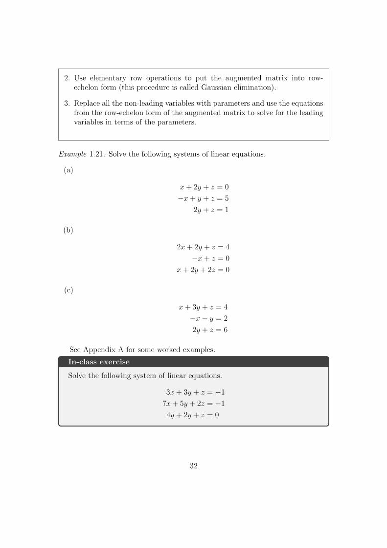
Example 1.21. Solve the following systems of linear equations.
(a)
x+ 2y + z = 0
−x+ y + z = 5
2y + z = 1
(b)
2x+ 2y + z = 4
−x+ z = 0
x+ 2y + 2z = 0
(c)
x+ 3y + z = 4
−x− y = 2
2y + z = 6
See Appendix A for some worked examples.
In-class exercise
Solve the following system of linear equations.
3x+ 3y + z = −1
7x+ 5y + 2z = −1
4y + 2y + z = 0
32
1.6 The rank of a matrix
It is a fact that if you start with a matrix A – no matter what order you performelementary row operations – you will always arrive at the same RREF matrix R.If you are interested, there is a proof of this fact at the end of Chapter 3. Onemight say,
“All roads (constructed from row operations) lead to the same reduced rowechelon form matrix.”
Because of this fact, we can make the following definition.
Definition 1.22. The rank of a matrix A is the number of leading entries (orpivots) in any row-echelon form of the matrix. We denote this number by rank(A).
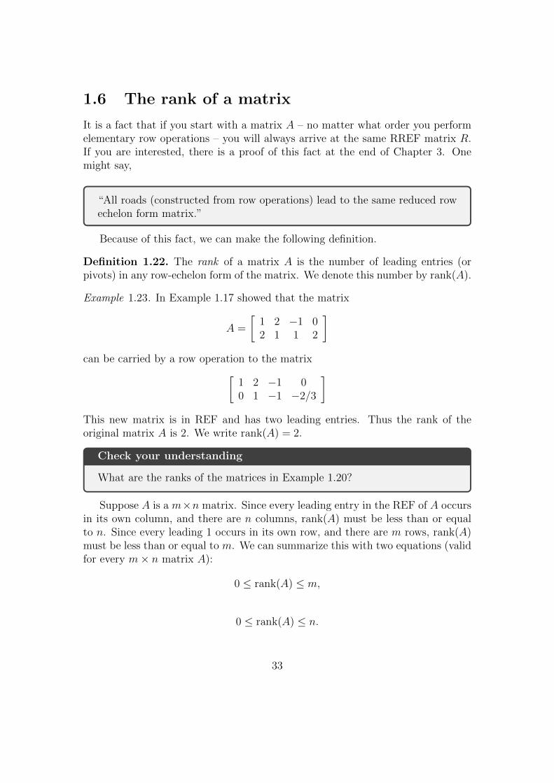
Example 1.23. In Example 1.17 showed that the matrix
A =
[1 2 −1 02 1 1 2
]can be carried by a row operation to the matrix[
1 2 −1 00 1 −1 −2/3
]This new matrix is in REF and has two leading entries. Thus the rank of theoriginal matrix A is 2. We write rank(A) = 2.
Check your understanding
What are the ranks of the matrices in Example 1.20?
Suppose A is a m×n matrix. Since every leading entry in the REF of A occursin its own column, and there are n columns, rank(A) must be less than or equalto n. Since every leading 1 occurs in its own row, and there are m rows, rank(A)must be less than or equal to m. We can summarize this with two equations (validfor every m× n matrix A):
0 ≤ rank(A) ≤ m,
0 ≤ rank(A) ≤ n.
33

Check your understanding
Suppose [A|b] is the augmented matrix of a system of 3 linear equations in4 variables.
What are the possible values of rank(A)?
What are the possible values of rank([A|b])?
In-class exercise
Suppose [A|b] is the augmented matrix of a system of m linear equations inn variables. If we know that rank([A|b]) = n + 1, what can we say aboutthe solutions of the system of equations?
Recall that every consistent system of linear equations has exactly one solutionor infinitely many solutions. Rank is useful because it helps us to distinguishbetween these two cases.
Theorem 1.24. Suppose [A|b] is the augmented matrix of a system of m lin-ear equations in n variables and let r denote the rank of [A|b]. If the system isconsistent, then
a) If r = n, the system has exactly one solution.
b) If r < n, the system has infinitely many solutions.
Proof. If r = n, then every variable is a leading variable, so there is exactly onesolution. If r < n, then there is at least one non-leading variable, so the set ofsolutions has at least one parameter, so there are infinitely many solutions.
Example 1.25. (a) The augmented matrix[1 0 00 0 1
]has rank 2. The corresponding system of linear equations is inconsistent.
(b) The augmented matrix [1 0 20 1 3
]has rank 2. The corresponding system of linear equations is consistent andhas exactly one solution.
34

(c) The augmented matrix [1 2 30 0 0
]has rank 1. The corresponding system of linear equations is consistent andhas infinitely many solutions.
(d) The augmented matrix [0 0 10 0 0
]has rank 1. The corresponding system of linear equations is inconsistent.
1.7 Discussion: linear and nonlinear problems in
science and mathematics
Key concepts from Chapter 1
Linear and non-linear equations, systems of linear equations, solutions ofsystems of equations, the augmented matrix of a system of linear equations,the coefficient matrix of a system of linear equations, the definition of amatrix, elementary row operations do not change the set of solutions of asystem of linear equations, Gaussian elimination, row-echelon form, the re-duced row-echelon form of a matrix, the rank of a matrix, the possible numberof solutions of a system of linear equations.
35

Chapter 2
Matrix algebra
In highschool algebra, you learned about operations on real numbers (addition,multiplication and division) and the properties of these operations. For example,you may have learned that for any numbers x, y, and z,
xy = yx
andx(y + z) = xy + xz.
These properties are the rules of basic algebra.
These properties are useful in many ways. For instance, one can use them tosimplify algebraic expressions using BEDMAS rules (brackets, exponents, division,multiplication, addition, subtraction). If a and b are numbers, then:
5(3a+ 2b+ (6a− a)) = 5(3a+ 2b+ 5a)
= 5(8a+ 2b)
= 40a+ 10b.
Recall that a m× n matrix is a rectangular array of numbers and/or variablesthat has m rows and n columns.
a11 a12 · · · a1na21 a22 · · · a2n
...am1 am2 · · · amn
We have already seen how matrices are useful in studying solutions to systems
of linear equations: the augmented matrix is a nice shorthand way to record the
36
information of a system of linear equations when performing Gaussian elimination.
In fact, the usefulness of matrices in studying systems of linear equations ismuch greater. One can define various operations for matrices (analogous to op-erations like multiplication and addition of numbers), and these operations areintimately related to the study of systems of linear equations.
In this chapter, we introduce operations on matrices. As in highschool algebra,operations on matrices have various properties. The rules for these operations arematrix algebra.
2.1 Equality of matrices
Before defining operations on matrices, we should carefully explain what it meansfor two matrices to be equal.
Two m× n matrices
A =
a11 a12 · · · a1na21 a22 · · · a2n
...am1 am2 · · · amn
and B =
b11 b12 · · · b1nb21 b22 · · · b2n
...bm1 bm2 · · · bmn
are equal if all of their entries are equal. This means that
aij = bij
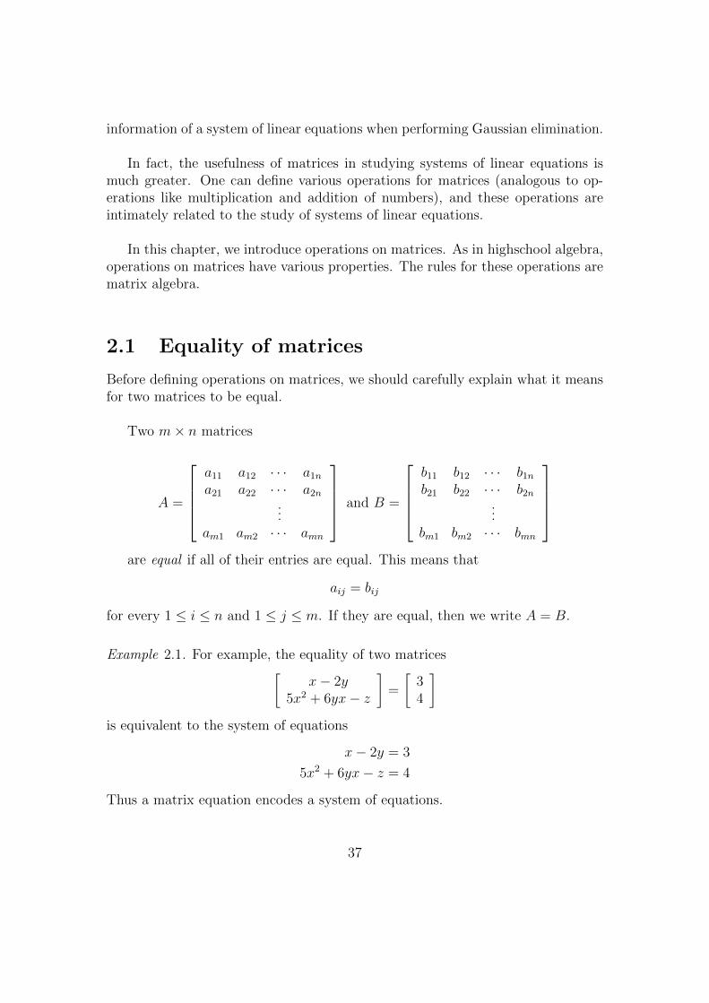
for every 1 ≤ i ≤ n and 1 ≤ j ≤ m. If they are equal, then we write A = B.
Example 2.1. For example, the equality of two matrices[x− 2y
5x2 + 6yx− z
]=
[34
]is equivalent to the system of equations
x− 2y = 3
5x2 + 6yx− z = 4
Thus a matrix equation encodes a system of equations.
37

Check your understanding
Consider the matrices
A =
[1 0 x2 6 x2
], B =
[1 0 12 6 1
], C =
[1 02 6
]For what values of x is A = B? For what values of x is A = C?
2.2 Matrix addition and scalar multiplication
The sum of two m× n matrices
A =
a11 a12 · · · a1na21 a22 · · · a2n
...am1 am2 · · · amn
and B =
b11 b12 · · · b1nb21 b22 · · · b2n
...bm1 bm2 · · · bmn
is the m× n matrix
A+B :=
a11 + b11 a12 + b12 · · · a1n + b1na21 + b21 a22 + b22 · · · a2n + b1n
...am1 + bm1 am2 + bm2 · · · amn + bmn
In other words, the ij entry of A+B is aij + bij, the sum of the ij entry of A andthe ij entry of B. Another name for this operation is matrix addition.
Example 2.2. For example,
• [13
]+
[1−1
]=
[22
]• The formula for the sum of two arbitrary 2× 2 matrices is[
a11 a12a21 a22
]+
[b11 b12b21 b22
]=
[a11 + b11 a12 + b12a21 + b21 a22 + b22
]
38

Example 2.3. Let 0m×n denote the m × n matrix whose entries are all zero. Wecall this the zero matrix . The matrix 0m×n has the special property that for anyother m× n matrix A,
A+ 0m×n = 0m×n + A = A.
The scalar multiplication of real number (or variable) k and a m× n matrix
A =
a11 a12 · · · a1na21 a22 · · · a2n
...am1 am2 · · · amn
is the m× n matrix
kA :=
ka11 ka12 · · · ka1nka21 ka22 · · · ka2n
...kam1 kam2 · · · kamn
In other words, the entries of kA are simply k times the entries of A, kaij.
Check your understanding
Let u =
[13
]and v =
[1−1
]. Compute the vector
u− 3v.
Properties of matrix addition and scalar multiplication
If A and B are m× n matrices and k, l are real numbers. Then,
(a) (scalar multiplication distributes over matrix addition)
k(A+B) = kA+ kB
(b) (scalar multiplication distributes over scalar addition)
(k + l)A = kA+ lA
39
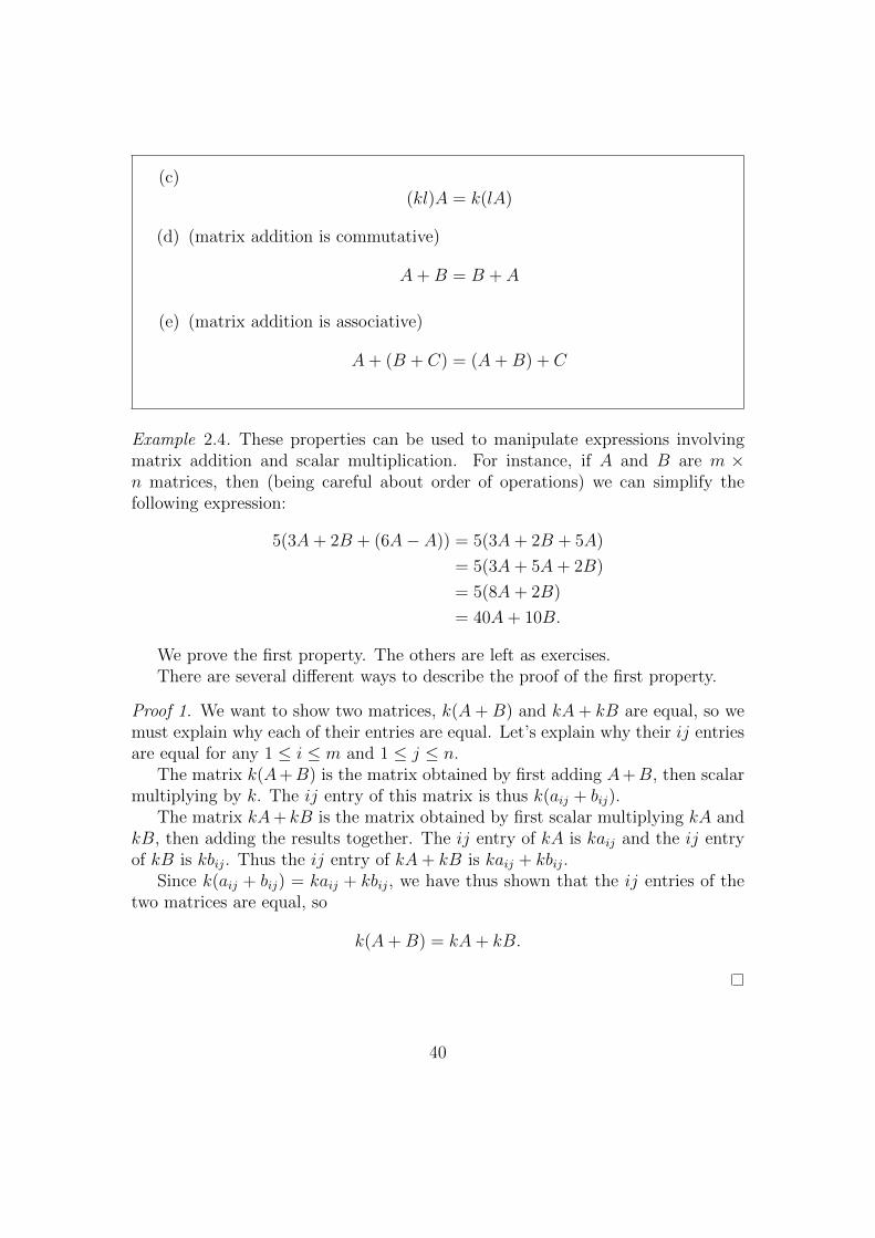
(c)(kl)A = k(lA)
(d) (matrix addition is commutative)
A+B = B + A
(e) (matrix addition is associative)
A+ (B + C) = (A+B) + C
Example 2.4. These properties can be used to manipulate expressions involvingmatrix addition and scalar multiplication. For instance, if A and B are m ×n matrices, then (being careful about order of operations) we can simplify thefollowing expression:
5(3A+ 2B + (6A− A)) = 5(3A+ 2B + 5A)
= 5(3A+ 5A+ 2B)
= 5(8A+ 2B)
= 40A+ 10B.
We prove the first property. The others are left as exercises.There are several different ways to describe the proof of the first property.
Proof 1. We want to show two matrices, k(A+B) and kA+ kB are equal, so wemust explain why each of their entries are equal. Let’s explain why their ij entriesare equal for any 1 ≤ i ≤ m and 1 ≤ j ≤ n.
The matrix k(A+B) is the matrix obtained by first adding A+B, then scalarmultiplying by k. The ij entry of this matrix is thus k(aij + bij).
The matrix kA+ kB is the matrix obtained by first scalar multiplying kA andkB, then adding the results together. The ij entry of kA is kaij and the ij entryof kB is kbij. Thus the ij entry of kA+ kB is kaij + kbij.
Since k(aij + bij) = kaij + kbij, we have thus shown that the ij entries of thetwo matrices are equal, so
k(A+B) = kA+ kB.
40

This is pretty wordy. We can write down most of this argument by introducingthe following shorthand. We write A = [aij]m×n to mean the matrix A equals them× n matrix with entries aij. The proof above can then be written more brieflyas follows.
Proof 2. Suppose A = [aij]m×n and B = [bij]m×n. Then by definition of matrixaddition and scalar multiplication,
k(A+B) = k ([aij]m×n + [bij]m×n) = k[aij + bij]m×n = [k(aij + bij)]m×n
and
kA+ kB = k[aij]m×n + k[bij]m×n = [kaij]m×n + [kbij]m×n = [kaij + kbij]m×n
Since k(aij + bij) = kaij + kbij,
[k(aij + bij)]m×n = [kaij + kbij]m×n.
Thus we have shown that
k(A+B) = kA+ kB.
Let’s write an even shorter version of this proof.
Proof 3. Let A = [aij] and B = [bij]. Let’s drop the []m×n from the notation, sincewe know all the matrices are m× n.
We start with k(A+B) and manipulate the formulas until we get to kA+ kB.
k(A+B) = k ([aij] + [bij])
= k[aij + bij] By definition of matrix addition.
= [k(aij + bij)] By definition of scalar multiplication.
= [kaij + kbij] Since multiplication distributes over addition.
= [kaij] + [kbij] By definition of matrix addition.
= k[aij] + k[bij] By definition of scalar multiplication.
= kA+ kB
41

2.3 Matrix-vector products
Given a m× n matrix
A =
a11 a12 · · · a1na21 a22 · · · a2n
...am1 am2 · · · amn
and a n× 1 column vector
x =
x1x2...xn
the matrix-vector product of A and x is the m× 1 column vector
Ax :=
a11x1 + a12x2 + · · ·+ a1nxna21x1 + a22x2 + · · ·+ a2nxn
...am1x1 + am2x2 + · · ·+ amnxn
Warning
The matrix-vector product Ax is only defined if the number of columns ofA equals the number of rows of x. Otherwise writing Ax has no meaning!
Example 2.5. Let’s compute a matrix vector product for practice.[1 0 42 6 −1
] 1−12
=
[1 · 1 + 0 · (−1) + 4 · 2
2 · 1 + 6 · (−1) + (−1) · 2
]=
[9−6
]
Example 2.6. If a = [a1 a2 . . . an] is a 1× n row vector and x is the n× 1 columnvector above, then the matrix-vector product
ax = [a1 a2 . . . an]
x1x2...xn
= [a1x1 + a2x2 + · · ·+ anxn] .
42

The result on the right hand side is a 1 × 1 matrix. We often think of a 1 × 1matrix as a real number and omit the brackets.
There are two useful ways to think about matrix-vector products. SupposeA is a m× n matrix as above.
• Suppose that ai = [ai1 ai2 . . . ain] are the rows of A. The formula formatrix vector products and the computation in the previous exampletell us that
Ax =
a11x1 + a12x2 + · · ·+ a1nxna21x1 + a22x2 + · · ·+ a2nxn
...am1x1 + am2x2 + · · ·+ amnxn
=
a1xa2x...
amx
• Suppose that
cj =
a1ja2j...amj
are the columns of A. Using sums and scalar multiples we can rewritethe matrix-vector product
Ax =
a11x1 + a12x2 + · · ·+ a1nxna21x1 + a22x2 + · · ·+ a2nxn
...am1x1 + am2x2 + · · ·+ amnxn
=
a11x1a21x1...
am1x1
+
a12x2a22x2...
am2x2
+ · · ·+
a1nxna2nxn...
amnxn
= x1
a11a21...am1
+ x2
a12a22...am2
+ · · ·+ xn
a1na2n...
amn
= x1c1 + x2c2 + · · ·+ xncn.
43

Properties of matrix-vector multiplication
Suppose that A and B are m× n matrices, k and l are real numbers, andu and v are n× 1 column vectors. Then,
(a)(A+B)u = Au +Bu
(b)A(u + v) = Au + Av
(c)k(Au) = A(ku)
Proof. We prove the second property, the others are exercises.
Using the second interpretation of the matrix-vector product above, we seethat
A(u + v) = A
u1 + v1...
un + vn
= (u1 + v1)a1 + · · · (un + vn)an
= (u1a1 + · · ·+ unan) + · · ·+ (v1a1 + · · · vnan)
= Au + Av.
In-class exercise
Let A and B be m× n matrices, and let u and v be n× 1 column vectors.Simplify the expression.
(A+B)(u + v)−Bu + 2Av
44

2.4 Matrix multiplication
Given a m× n matrix
A =
a11 a12 · · · a1na21 a22 · · · a2n
...am1 am2 · · · amn
and a n× p matrix
B =
b11 b12 · · · b1pb21 b22 · · · b2p
...bn1 bn2 · · · bnp
=[
b11 b12 · · · b1p
]
where
bj =
b1jb2j...bnj
are the columns of B, the product , A times B, is the m× p matrix AB whose jthcolumn is the matrix vector product Abj. Explicitly,
AB :=[Ab1 Ab2 · · · Abp
]The ijth entry of this matrix is the ith entry of the matrix-vector product Abj,which equals
n∑k=1
aikbkj = ai1b1j + ai2b2j + · · ·+ ainbnj.
In-class exercise
Suppose
A =
[1 12 −1
], B =
[0 2 1−1 1 0
].
Compute the product AB.
45
Warning
The product AB is only defined if the number of columns of A equals thenumber of rows of B. Otherwise writing AB has no meaning!
For example, in the preceding exercise, we can compute AB, but not BA,since B has three columns and A has two rows.
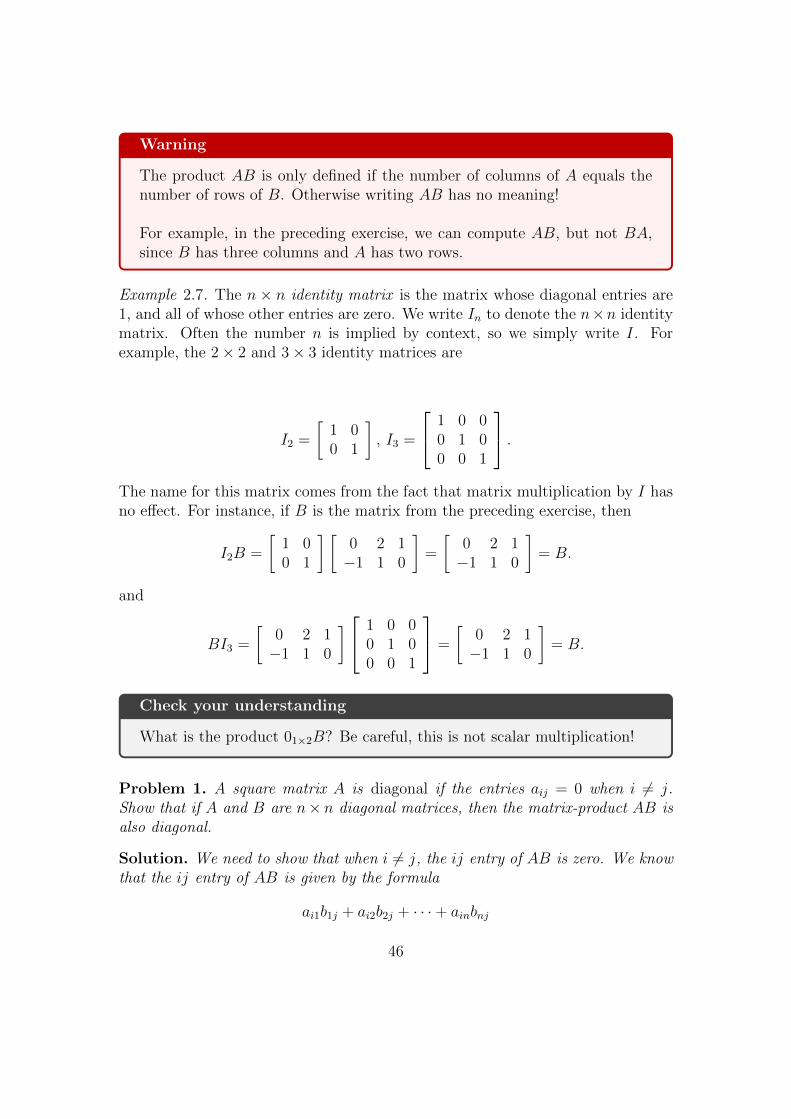
Example 2.7. The n × n identity matrix is the matrix whose diagonal entries are1, and all of whose other entries are zero. We write In to denote the n×n identitymatrix. Often the number n is implied by context, so we simply write I. Forexample, the 2× 2 and 3× 3 identity matrices are
I2 =
[1 00 1
], I3 =
1 0 00 1 00 0 1
.The name for this matrix comes from the fact that matrix multiplication by I hasno effect. For instance, if B is the matrix from the preceding exercise, then
I2B =
[1 00 1
] [0 2 1−1 1 0
]=
[0 2 1−1 1 0
]= B.
and
BI3 =
[0 2 1−1 1 0
] 1 0 00 1 00 0 1
=
[0 2 1−1 1 0
]= B.
Check your understanding
What is the product 01×2B? Be careful, this is not scalar multiplication!
Problem 1. A square matrix A is diagonal if the entries aij = 0 when i 6= j.Show that if A and B are n× n diagonal matrices, then the matrix-product AB isalso diagonal.
Solution. We need to show that when i 6= j, the ij entry of AB is zero. We knowthat the ij entry of AB is given by the formula
ai1b1j + ai2b2j + · · ·+ ainbnj
46

where [ai1 ai2 · · · ain] is the ith row of A andb1jb2j...bnj
is the jth column of B.
• Since A is diagonal, all the entries in the ith row of A are zero except aii.
• Since B is diagonal, all the entries in the jth row of B are zero except bjj.
Thus the formula for the ij entry of AB looks like
0 + · · ·+ 0 + aiibij + 0 + · · ·+ 0 + aijbjj + 0 + · · ·+ 0
if i 6= j. But bij = 0 and aij = 0, so the ij entry is
0 + · · ·+ 0 + aii0 + 0 + · · ·+ 0 + 0bjj + 0 + · · ·+ 0 = 0. �
Properties of matrix multiplication
Suppose that A, B and C matrices. Then, whenever the operations beloware defined,
(a) (left distributivity)A(B + C) = AB + AC
(b) (right distributivity)
(A+B)C = AC +BC
(c)k(AB) = (kA)B = A(kB)
(d) (associativity)A(BC) = (AB)C
47

Proof. (a) Let bj denote the columns of B and let cj denote the columns of B.Then,
A(B + C) = A[b1 + c1 · · · bp + cp]
= [A(b1 + c1) · · · A(bp + cp)]
= [Ab1 + Ac1 · · · Abp + Acp] By prop. of mat-vect mult.
= [Ab1 · · · Abp] + [Ac1 · · · Acp]
= A[b1 · · · bp] + A[c1 · · · cp]= AB + AC.
(b) Exercise.
(c) Exercise.
(d) Unravelling the definitions, we see that the ij entry of (AB)D is
p∑l=1
(n∑k=1
aikbkl
)dlj
whereas the ij entry of A(BD) is
n∑k=1
aik
(p∑l=1
bkldlj
).
These two sums are equal, so the ij entries are equal.
Because of property (d), we know that for any square matrix A, A(AA) =(AA)A. Thus it is ok to simply write AAA because the order in which you multiplythe matrices doesn’t matter. We write A3 = AAA for short. In general, we usethe notation Ak to mean the product of A by itself k-times.
Ak = A · A · · ·A.
48

2.5 Matrix transpose
The transpose of a m× n matrix
A =
a11 a12 · · · a1na21 a22 · · · a2n
...am1 am2 · · · amn
is the n×m matrix
AT :=
a11 a21 · · · am1
a12 a22 · · · am2
...a1n a2n · · · amn
In plain english, the transpose of A is the matrix AT whose rows are the columnsof A and whose columns are the rows of A.
This is best illustrated with examples.
Example 2.8. Consider the matrices
A =
1 21 56 3
, B =
0 2 91 5 π6 8 e
, u =
0−15
,The definition of matrix transpose tells us that
AT =
[1 1 62 5 3
], BT =
0 1 62 5 89 π e
, uT =[
0 −1 5],
Remark 2.9. Observe that
• The transpose of a square matrix is a square matrix.
• The transpose of a column vector (a m× 1 matrix) is a row vector (a 1×mmatrix).
• The transpose of a row vector (a 1×m matrix) is a column vector (a m× 1matrix).
49

• Since the transpose AT of a m × n matrix A is a n × m matrix, one canalways compute the matrix products
AAT and ATA.
Check your understanding
If A is a n ×m matrix, how many rows and columns do the matrices AAT
and ATA have?
In-class exercise
Suppose A is a n×m matrix and AT is its transpose. What is the transposeof AT ?
Properties of matrix transpose
Suppose that A and B are m× n matrices, C is a n× p matrix, and k is anumber. Then,
(a)(A+B)T = AT +BT
(b)(AC)T = CTAT
(c)kAT = (kA)T
(d)(AT )T = A
Proof. (a) We write our explanation using our shorthand for matrices.
(A+B)T = [aij + bij]Tm×n
= [aji + bji]n×m
= [aji]n×m + [bji]n×m
= AT +BT .
(b) Exercise.
50

(c) Exercise.
(d) Using matrix shorthand, the proof is very brief:
(AT )T =([aij]
T)T
= ([aji])T = [aji]
T = [aij] = A
In-class exercise
Explain each step in the proof of property (a).
2.6 Matrix equations
Now that we have defined what it means for two matrices to be equal, and we haveintroduced various operations on matrices, we can study matrix equations.
Example 2.10. Suppose
A =
[1 −10 4
], and B =
[1 00 3
]and
X =
[x11 x12x21 x22
]where xij are variables. The matrix equation
A+ 2X = B
can be written explicitly as the equality of matrices[1 + 2x11 −1 + 2x120 + 2x21 4 + 2x22
]=
[1 00 3
]Since two matrices are equal when their entries are equal, this equation is truewhen the variables xij satisfy the system of equations
1 + 2x11 = 1
−1 + 2x12 = 0
0 + 2x21 = 0
4 + 2x22 = 3
Thus, the problem of solving this particular matrix equation reduces to a systemof linear equations.
51

Now suppose that
A =
a11 a12 · · · a1na21 a22 · · · a2n
...am1 am2 · · · amn
, and b =
b1b2...bm
are matrices whose entries are the constants, aij and bi, and
x =
x1x2...xn
is a n× 1 column vector whose entries are variables x1, . . . , xn.
In-class exercise
Use the matrix vector product to expand the matrix-vector equation
Ax = b.
What is the resulting system of equations?
Which column vectors x solve the matrix equation?
Note that matrix equations can also define a system of equations that is notlinear. See Tutorial 3.
2.7 Discussion: non-commuting operators and
quantum mechanics
Key concepts from Chapter 2
Equality of matrices, matrix addition and scalar multiplication, matrix-vector multiplication, matrix multiplication, matrix transpose, all the prop-erties of these operations. Matrix equations. Writing a system of linearequations as a matrix equation
52

Chapter 3
More systems of linear equations
In Chapter 1 we introduced systems of linear equations and in Chapter 2 we intro-duced operations on matrices: addition, scalar multiplication, and multiplication.In this chapter we show how matrix algebra can be used to study systems of linearequations, and vis versa.
3.1 The matrix equation of a system of linear
equations
Recall that solutions of a system of m linear equations in n variables
a11x1 + a12x2 + · · · + a1nxn = b1a21x1 + a22x2 + · · · + a2nxn = b2
...am1x1 + am2x2 + · · · + amnxn = bm
(3.1)
are n-tuples of numbers (s1, . . . , sn) that solve every equation in the system. i.e.
ai1s1 + ai2s2 + · · ·+ ainsn = bi
for every 1 ≤ i ≤ m.
Now suppose that
A =
a11 a12 · · · a1na21 a22 · · · a2n
...am1 am2 · · · amn
, and b =
b1b2...bm
53

are the coefficient matrix and constant matrix of the system, and let
x =
x1x2...xn
be the n× 1 column vector whose entries are the variables x1, . . . , xn.
In Section 2.6, we discovered that a vector
s =
s1s2...sn
solves the matrix equation of the system (3.1),
Ax = b (3.2)
if and only if, the n-tuple (s1, . . . , sn) solves the system of linear equations (3.1).
In other words, the problem of solving the system of linear equations, (3.1) andthe problem of solving the matrix equation (3.2) are one and the same!
For this reason, it is common to refer to the equation Ax = b as a “systemof linear equations” even though it is a matrix equation. It encodes a system oflinear equations.
As a consequence of this fact, we can use all the nice operations of matrixalgebra to study (and prove facts about) systems of linear equations and vis versa!This is one of the main themes of this chapter.
Check your understanding
Write the matrix equation corresponding to the system of linear equations
x + 2y − z = 02x + y + z = 2
54

3.2 Span and systems of linear equations
Recall that the matrix vector product Ax can be expanded as
Ax = x1
a11a21...am1
+ x2
a12a22...am2
+ · · ·+ xn
a1na2n...
amn
.Thus we see that
The following two statements are equivalent:
• The system Ax = b is consistent.
• There are numbers t1, . . . , tn such that
t1
a11a21...am1
+ t2
a12a22...am2
+ · · ·+ tn
a1na2n...
amn
=
b1b2...bm
For the remainder of this section, we denote the column vectors of A by
aj =
a1ja2j...amj
.Definition 3.3. Any expression of the form
t1a1 + t2a2 + · · ·+ tnan
where ti ∈ R and aj are column vectors is called a linear combination of the columnvectors a1, . . . , an.
55
Check your understanding
Let u =
[13
]and v =
[1−1
]. Can the vector
[−26
]be written as a linear combination of u and v?
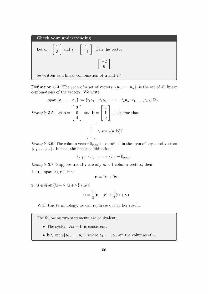
Definition 3.4. The span of a set of vectors, {a1, . . . , an}, is the set of all linearcombinations of the vectors. We write
span {a1, . . . , an} := {t1a1 + t2a2 + · · ·+ tnan : t1, . . . , tn ∈ R} .
Example 3.5. Let a =
204
and b =
210
. Is it true that
111
∈ span{a,b}?
Example 3.6. The column vector 0m×1 is contained in the span of any set of vectors{a1, . . . , an}. Indeed, the linear combination
0a1 + 0a2 + · · ·+ 0an = 0m×1.
Example 3.7. Suppose u and v are any m× 1 column vectors, then
1. u ∈ span {u,v} sinceu = 1u + 0v.
2. u ∈ span {u− v,u + v} since
u =1
2(u− v) +
1
2(u + v).
With this terminology, we can rephrase our earlier result:
The following two statements are equivalent:
• The system Ax = b is consistent.
• b ∈ span {a1, . . . , an}, where a1, . . . , an are the columns of A.
56

In-class exercise
Use what we know about solving systems of linear equations to determinewhether 1
11
∈ span
1−11
, 1
00
, 1
02
.
3.3 Homogeneous systems of linear equations
A system of linear equations is called homogeneous if all the constant terms arezero:
a11x1 + a12x2 + · · · a1nxn = 0a21x1 + a22x2 + · · · a2nxn = 0
...am1x1 + am2x2 + · · · amnxn = 0
The augmented matrix of a homogeneous system has a column of zeros:a11 a12 · · · a1n 0a21 a22 · · · a2n 0
...am1 am2 · · · amn 0
The matrix equation of a homogeneous system is
Ax = 0
where 0 = 0m×1 is the m× 1 column vector of zeros.
Homogeneous systems of linear equations are important for several reasons.The first reason is the following fact:
Every homogeneous system of linear equations is consistent.
Just as important as this fact is the reason why it’s true: every homogeneoussystem has the trivial solution, x1 = 0, x2 = 0, . . . , xn = 0.
57

In-class exercise
Consider the following statement:
If a homogeneous system of linear equations has more variables thanequations, then it must have infinitely many solutions.
Why is this true? (think back to Chapter 1)
If you remove the word “homogeneous”, then the statement is false. Why?
3.4 Linear combinations and basic solutions
If u and v are two solutions of a homogeneous matrix equation Ax = 0, then wecan use matrix algebra to show that u + v is also a solution:
A(u + v) = Au + Av = 0 + 0 = 0.
In fact, even more is true. If t and r are any real numbers, then we can showthat tu + rv is also a solution:
A(tu + rv) = A(tu) + A(rv) = t(Au) + r(Av) = t0 + r0 = 0.
While we are at it, why stop at only two solutions? If we have k solutions tothe equation, u1, . . . ,uk, and k real numbers t1, . . . , tk, then the vector
t1u1 + t2u2 + . . .+ tkuk
is also a solution! We use the same matrix algebra steps as before:
A (t1u1 + t2u2 + . . .+ tkuk) = A (t1u1) + A (t2u2) + . . .+ A (tkuk)
= t1Au1 + t2Au2 + · · ·+ tkAuk
= t10 + t20 + · · ·+ tk0
= 0
The expressiont1u1 + t2u2 + . . .+ tkuk
is called a linear combination of the vectors u1, . . . ,uk. In the preceding calcula-tion, we have proven the following fact:
58
Every linear combination of solutions to a homogeneous system of linearequations is a solution.
Check your understanding
The fact that the matrix equation/system is homogeneous is crucial. Indeed,suppose that we have a non-homogeneous matrix equation
Ax = b
where b is non-zero.
Suppose that u and v are solutions to this matrix equation. Use matrixalgebra to simplify the expression
A(u + v).
Is u + v a solution of the matrix equation?
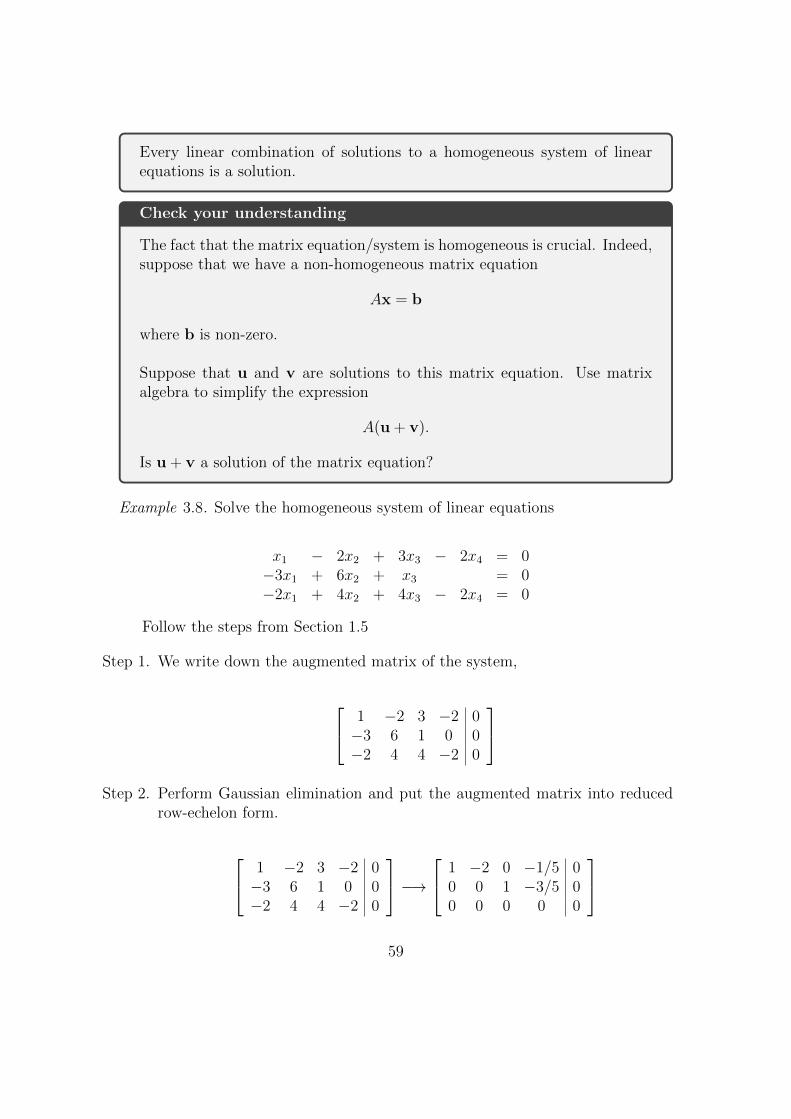
Example 3.8. Solve the homogeneous system of linear equations
x1 − 2x2 + 3x3 − 2x4 = 0−3x1 + 6x2 + x3 = 0−2x1 + 4x2 + 4x3 − 2x4 = 0
Follow the steps from Section 1.5
Step 1. We write down the augmented matrix of the system,
1 −2 3 −2 0−3 6 1 0 0−2 4 4 −2 0
Step 2. Perform Gaussian elimination and put the augmented matrix into reduced
row-echelon form.
1 −2 3 −2 0−3 6 1 0 0−2 4 4 −2 0
−→ 1 −2 0 −1/5 0
0 0 1 −3/5 00 0 0 0 0
59

Step 3. Introduce parameters x2 = t1 and x4 = t2 for the non-leading variables.From the reduced row-echelon form, we read the equations
x1 = 2t1 +1
5t2
x2 = t1
x3 =3
5t2
x4 = t2
We can write these equations using sums and scalar multiples of columnvectors:
x1x2x3x4
=
2t1 + 1
5t2
t135t2t2
= t1
2100
+ t2
15
035
1
Thus, the set of all solutions to the linear system above can be described asthe set of all vectors
t1
2100
+ t2
15
035
1
where t1 and t2 are any real numbers. (you can also describe the solutionsas n-tuples). In set-builder notation, we writet1
2100
+ t2
15
035
1
: t1, t2 ∈ R
Definition 3.9. Given a system of linear equations whose augmented matrix is inreduced row-echelon form, the basic solutions are the vectors obtained by settingall of the free variables to be zero except for one.
In the previous example, the basic solutions to the system of linear equationsare the column vectors
2100
,
15
035
1
.60
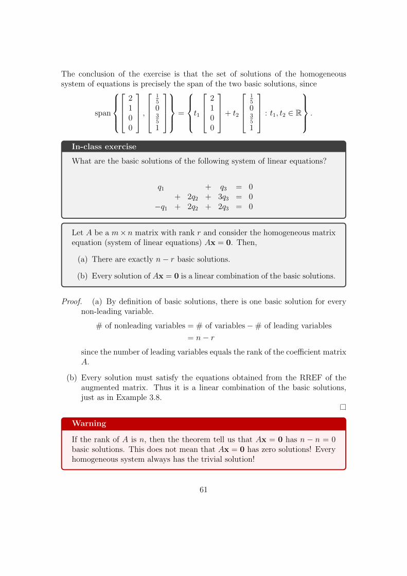
The conclusion of the exercise is that the set of solutions of the homogeneoussystem of equations is precisely the span of the two basic solutions, since
span
2100
,
15
035
1
=
t1
2100
+ t2
15
035
1
: t1, t2 ∈ R
.
In-class exercise
What are the basic solutions of the following system of linear equations?
q1 + q3 = 0+ 2q2 + 3q3 = 0
−q1 + 2q2 + 2q3 = 0
Let A be a m×n matrix with rank r and consider the homogeneous matrixequation (system of linear equations) Ax = 0. Then,
(a) There are exactly n− r basic solutions.
(b) Every solution of Ax = 0 is a linear combination of the basic solutions.
Proof. (a) By definition of basic solutions, there is one basic solution for everynon-leading variable.
# of nonleading variables = # of variables−# of leading variables
= n− r
since the number of leading variables equals the rank of the coefficient matrixA.
(b) Every solution must satisfy the equations obtained from the RREF of theaugmented matrix. Thus it is a linear combination of the basic solutions,just as in Example 3.8.
Warning
If the rank of A is n, then the theorem tell us that Ax = 0 has n − n = 0basic solutions. This does not mean that Ax = 0 has zero solutions! Everyhomogeneous system always has the trivial solution!
61

Problem 2. Let A be the matrix1 −3 0 2 2−2 6 1 2 −53 −9 −1 0 7−3 9 2 6 −8
Write the set of solutions to the system of equations Ax = 0 as the span of a setof vectors.
Solution. Step 1: Row reduce the matrix until it is in reduced row echelon form.1 −3 0 2 2−2 6 1 2 −53 −9 −1 0 7−3 9 2 6 −8
→ · · · →
1 −3 0 2 20 0 1 6 −10 0 0 0 00 0 0 0 0
Step 2: The free variables are x2, x4, x5. Compute the basic solutions by setting
one free variable to be 1 and the others to be zero, then back substituting.31000
,−20−610
,−20101
Step 3: Write
span
31000
,−20−610
,−20101
.
3.5 The associated homogeneous system of lin-
ear equations
Suppose we have a system of linear equations whose matrix equation is Ax = b,and b is non-zero. This is not a homogeneous system, but there is an associatedhomogeneous system, Ax = 0, which is obtained simply by replacing b with 0.
The associated homogeneous system is interesting for the following reason.
62

Suppose u1 is a solution of Ax = b, we call this a particular solution. If u0
is a solution of the associated homogeneous system, then by properties of matrixalgebra,
A(u0 + u1) = Au0 + Au1 = 0 + b = b.
Thus we have shown that u0+u1 is also a solution of Ax = b. In fact, all solutionsof Ax = b can be written this way.
Theorem 3.10. Suppose u1 is a particular solution of a system Ax = b. Then,every solution of Ax = b can be written as
u1 + u0
for some solution u0 of the associated homogeneous system Ax = 0.
Proof. Suppose that v is an arbitrary solution of Ax = b. In other words, Av = b.
We must show that there is a u0 solving Ax = 0, such that v = u1 + u0.
We know that u1 is a solution of a system Ax = b. Thus, by matrix algebra,
A(v − u1) = Av − Au1 = b− b = 0.
This tells us that if we define u0 = v − u1, then u0 is a solution of Ax = 0.
But now we have found a solution u0 of Ax = 0 such that
v = u1 + u0.
This is what we wanted to do, so we are finished.
3.6 All roads lead to the same reduced row ech-
elon form
In this section (which is bonus material) we will give a short explanation of theimportant fact from Chapter 1,
“All roads (constructed from row operations) lead to the same reduced rowechelon form matrix.”
63

In other words, we want to prove the following statement: If C is a matrix thatcan be carried to reduced row echelon form matrices A and B by row operations,then A = B.
We will prove this in a number of steps.
(a) First of all, if C = 0 then C = A = B. Thus we assume for the rest of theproof that C has some nonzero entries.
(b) Since we can go C → A by row operations and C → B by row operations, andwe know that all row operations can be reversed, then we can go A→ C → Busing row operations.
(c) The first pivot column of A and B must be the same (this is the first nonzerocolumn from the left, which has a 1 in the top entry and zeros below it).This is true because there is no way to eliminate the first pivot using rowoperations, and we can get from A to B by row operations.
(d) If A 6= B, then they differ in some entries. Let j be the index of the firstcolumn from the left where they don’t have the same entries. Let’s write afor the jth column of A and b for the jth column of B.
(e) Delete all the columns of A and B to the right (with index j + 1 or larger)and all the non-pivot columns to the left. Now we have two new matrices,lets call them A′ and B′, with dimensions n × k (k ≤ j is the number ofpivot columns we kept). Both A′ and B′ are in reduced row echelon form,and they differ only in their last column.
(f) Since we deleted all the non-pivot columns to the left of column j, A′ andB′ are of the form A′ = [e1|e2|...|ek−1|a] and B′ = [e1|e2|...|ek−1|b].
(g) Since we can go A → B by row operations, we can go A′ → B′ by rowoperations. Thus, by Theorem 1.18, the systems of equations A′x = 0 andB′x = 0 have the same solutions.
(h) Exercise: Show that if [e1|e2|...|ek−1|a]x = 0 and [e1|e2|...|ek−1|b]x = 0 havethe same solutions, then a = b.
This is awkward. By part (d), we had assumed that a and b were the first columnsof A and B that were different, but we just used the fact that A and B are rowequivalent to explain that a = b. Where did this contradiction originally comefrom? It came from the beginning of part (d) where we wrote A 6= B! Since thislead to a contradiction, we must conclude that this is wrong. A = B as we wantedto show.
64

Key concepts from Chapter 3
The matrix equation of a system of linear equations, homogeneous systems,linear combinations, the span of a set of vectors, Ax = b is consistent ifand only if b is in the span of the columns of A, linear combinations of so-lutions to homogeneous systems are solutions, basic solutions, the associatedhomogeneous system, particular solutions.
65

Chapter 4
Matrix inverses
If a is a nonzero number, then there exists a number, b, such that
ab = 1
In fact, we know exactly what this number is, so this property is no surprise: b = 1a.
On the other hand, if a = 0, then there is no number b such that ab = 1, since
ab = 0b = 0.
In this chapter we are interested in understanding analogous properties for ma-trix multiplication. Let’s begin with some examples.
In-class exercise
Find u, v, w, z so that[1 10 −2
] [u vw z
]=
[1 00 1
]
In-class exercise
Suppose a, b, c, d are fixed. When is it possible to find u, v, w, z so that[a bc d
] [u vw z
]=
[1 00 1
]?
If you can find solutions for u, v, w, z, how many are there? Exactly one?Infinitely many?
66

These two exercises demonstrate the following phenomenon: for some matricesA, there exists a matrix B such that
AB = I
whereas for others there does not. This is similar to the situation in highschoolalgebra, but slightly more complicated. In this chapter, we study this phenomenonin more detail.
4.1 Invertible matrices
For the rest of this section A and B are n× n matrices.
Since it is not always true that AB = BA, the definition of “invertible” formatrices is a little bit complicated.
Definition 4.1. A n × n matrix A is invertible if there exists a n × n matrix Bsuch that
AB = I and BA = I.
Example 4.2. We give several examples of invertible and non-invertible matrices.
(a) A 1 × 1 matrix [a] is just a number. By the discussion at the beginning ofthe chapter, [a] is invertible if and only if a 6= 0.
(b) The identity matrices are invertible since
I2 = I.
(c) A diagonal matrix is a matrix of the form
D =
a11. . .
ann
where all the entries not along the diagonal are zero. If all of the diagonalentries a11, . . . , ann 6= 0, then D is invertible. Let B be the diagonal matrix
B =
1a11
. . .1ann
Then one can compute the matrix products DB = I and BD = I, so D isinvertible.
67

(d) As we saw in the introduction, suppose A is the 2× 2 matrix
A =
[a bc d
]where a, b, c, d are arbitrary numbers.
If ad− bc 6= 0, then we can define the matrix
B =1
ad− bc
[d −b−c a
](if ad− bc = 0, then this formula does not define a matrix B since we havedivided by 0). We can check that
AB =
[a bc d
](1
ad− bc
[d −b−c a
])=
[1 00 1
]and
BA =
(1
ad− bc
[d −b−c a
])[a bc d
]=
[1 00 1
]Thus, if ad− bc 6= 0, then A is invertible.
On the other hand, as we saw in the introduction to the chapter, if ad−bc = 0,then the matrix equation AB = I has no solutions, so A is not invertible.
(e) Suppose A has a row of zeros, say the ith row = 01×n. Then for any matrixB the ii entry of AB is 0. Thus A is not invertible.
(f) Similarly, if A has a column of zeros, say the jth column, then the jj entryof BA is 0, so A is not invertible.
4.2 The inverse of a matrix
If A is an invertible matrix, then we know that there is a matrix B such thatAB = BA = I. We saw in the previous section, that if a 2 × 2 matrix A isinvertible, then the matrix
B =1
ad− bc
[d −b−c a
]
68

satisfies the matrix equations AB = I and BA = I. In fact, the example from theintroduction to this chapter tells us that the matrix equation AB = I has exactlyone solution.
The same is true in general.
If A is invertible, then there exists a unique matrix B with the property thatAB = BA = I.
We call this unique matrix the inverse of A and denote it by A−1.
An object with a certain property is unique if it is the only object with thatproperty. Another way to say the same thing is “there is exactly one objectwith this property.”
For instance, in a large MAT223 lecture,
• There is a unique person in the room that is the instructor.
• There may be several people who share the first name “Jeremy.” Inthis case, there is not a unique person in the class with the first name“Jeremy.”
Proof. Suppose that B and C are n× n matrices such that CA = I and AB = I.Then by matrix algebra,
B = IB = (CA)B = C(AB) = CI = C.
Thus B = C.
If A is invertible, then the system Ax = b has a unique solution,
x = A−1b.
Proof. Suppose A is invertible. Then A(A−1b) = (AA−1)b = b so the equationAx = b has a solution, A−1b. In fact, A−1b is the only solution, since if u is asolution, then
Au = b⇒ A−1(Au) = A−1(b)⇒ u = A−1b
Thus, the matrix equation Ax = b has exactly one solution for all b.
69

We record several important properties of matrix inverses, which are a part ofmatrix algebra.
Properties of matrix inverses
If A and B are invertible n× n matrices, then
(a) If A is invertible, then AT is invertible and
(AT )−1 = (A−1)T .
(b) The product AB is invertible, and
(AB)−1 = B−1A−1
(c) If k 6= 0 then kA is invertible and
(kA)−1 =1
kA−1
(d) If A is invertible, then A−1 is invertible and
(A−1)−1 = A.
Proof. (a) By matrix algebra,
AT (A−1)T = (A−1A)T = (I)T = I
and(A−1)TAT = (AA−1)T = IT = I.
(b) Again, using matrix algebra, we see that
(AB)B−1A−1 = A(BB−1)A−1 = AIA−1 = AA−1 = I
andB−1A−1(AB) = B(AA−1)B−1 = BIB−1 = BB−1 = I
(c) Exercise.
70
(d) Since A is invertible, we know there is an inverse A−1 such that
AA−1 = I and A−1A = I.
By definition, these two equations tell us that the matrix A−1 is invertibleand the inverse of A−1 is A.
Check your understanding
Suppose that A, B and C are invertible n× n matrices.
Is the product ABC invertible?
In-class exercise
Prove property (c).
Warning
If A and B are invertible n×n matrices, it is not necessarily true that A+Bis invertible. This is true even when A and B are scalars: both 2 and −2are invertible, but 2− 2 = 0 is not invertible.
4.3 Elementary matrices
Example 4.3. Consider the 3× 3 matrices
E1 =
0 1 01 0 00 0 1
, E2 =
1 0 00 1 00 0 k
, and E3 =
1 0 k0 1 00 0 1
Let
B =
b11 b12 b13b21 b22 b23b31 b32 b33
71

In-class exercise
Compute the products
E1B, E2B, and E3B.
For each matrix product, solve the matrix equation EiB = I for the variablesbij.
Definition 4.4. An elementary matrix E is a matrix that is obtained by perform-ing a single elementary row operation on the identity matrix I.
Check your understanding
For each of the matrices E1, E2, E3 above, explain how to obtain Ei byperforming one elementary row operation on I.
For what values of k is E2 an elementary matrix?
Observe that the result of multiplying B on the left by an elementary matrixis the same as performing the corresponding elementary row operation on B.
If ER is an elementary matrix corresponding to an elementary row operationR, then for any n×m matrix B, the product EB equals the matrix obtainedfrom B by performing the row operation R.
Recall that every elementary row operation R can be reversed by another ele-mentary row operation. We denote the reverse/inverse row operation by R−1.
Every elementary matrix ER (corresponding to the row operation R) isinvertible, and E−1R = ER−1 is the elementary matrix corresponding to thereverse row operation.
Proof. By the preceding fact, we see that the matrix
ER−1ER = ER−1ERI
is the same as the matrix obtained from I by performing the row operation R,then performing the reverse row operation R−1. This sequence of row operationsgives us back I, so ER−1ER = I. Similarly, we can check that ERER−1 = I.
72

Check your understanding
Write the 3 × 3 elementary matrices corresponding to the following rowoperations:
(a) Interchange row 2 and 3.
(b) Interchange row 1 and 3.
(c) Add −2 times row 3 to row 2.
(d) Add −2 times row 2 to row 3.
(e) Multiply row 1 by 6.
What is the inverse of each elementary matrix?
In-class exercise
Suppose that E1, E2, . . . , Ek are elementary matrices.
The product Ek · · ·E2E1 is invertible. Why? What is its inverse?
4.4 The matrix inversion algorithm
Given a n×n matrix A, we can form a n× 2n matrix [A|I]. The matrix inversionalgorithm is the following.
The matrix inversion algorithm
The algorithm is simple: perform elementary row operations on the matrix[A|I] until A is in reduced row echelon form.
Once this is finished, there are two possibilities:
1. If the reduced row echelon form of A is I, then the resulting matrix is [I|A−1]
2. If the reduced row echelon form of A is not I, then A is not invertible.
Proof. Suppose R1, . . . , Rk is a sequence of elementary row operations that carry Ato its reduced row-echelon form. Since left multiplication by elementary matrices
73

corresponds to performing elementary row operations, we know that
Ek · · ·E2E1A
is in reduced row echelon form.
If the reduced row echelon form is I, then we know that
Ek · · ·E2E1A = I
This means that A is invertible, and A−1 = Ek · · ·E2E1. This is precisely thematrix that will show up on the right hand side of the block matrix [A|I] afterperforming elementary row operations.
If the reduced row echelon form is not I, then it must have a column of zeros.Thus by the examples in Section 4.1, the matrix
Ek · · ·E2E1A
is not invertible. It is possible to conclude from this that A is not invertible. SeeTutorial ??.
As a consequence of this proof, we also see the following. If A is invertible,then
A = (Ek · · ·E2E1)−1 = E−11 · · ·E−1k .
Since inverses of elementary matrices are elementary matrices, we have shown thefollowing useful fact.
Let A be a n× n matrix. The following statements are equivalent:
1. A is invertible.
2. A is equal to a product of elementary matrices.
Example 4.5. Use the matrix inversion algorithm to determine whether the follow-ing matrices are invertible and if so, find their inverses. 1 1 0
−1 0 11 0 0
, 0 1 0
1 2 10 1 0
If the matrix is invertible, write the matrix and its inverse as a product of elemen-tary matrices.
74

4.5 The big theorem for square matrices (part
1)
The pinnacle of the first four chapters of the course is the following theorem, whichdemonstrates how several different concepts are related.
Theorem 4.6. [The big theorem for square matrices, part 1] Suppose A is a n×nmatrix. The following statements are equivalent:
(a) The matrix A is invertible.
(b) The matrix equation Ax = b has exactly one solution for all n × 1 columnvectors b.
(c) The homogeneous matrix equation Ax = 0 has exactly one solution (thetrivial solution).
(d) The rank of A is n.
(e) The reduced row-echelon form of A is I.
(f) There exists a n× n matrix B such that AB = I.
(g) There exists a n× n matrix B such that BA = I.
(h) A can be written as a product of elementary matrices.
“the following statements are equivalent” means that if any one of thesethings are true, then the others are also true. For instance, if you know that(d) is true, then you can conclude that (a) is true.
Proof. Let’s prove that (a)-(e) are equivalent. In the next section we will finishthe proof by showing that (a), (f), and (g) are equivalent. The fact that (a) and(h) are equivalent was explained in the previous section.
(a)⇒ (b) This was already proven in Section 4.1.
(b)⇒ (c) Suppose the matrix equation Ax = b has exactly one solution for allb. Then, in particular, it has exactly one solution when b = 0.
75

(c) ⇒ (d) Suppose that Ax = 0 has exactly one solution. Then by Theorem1.24, the rank of A must equal n.
(d)⇒ (e) If the rank of A is n, then the reduced row echelon form of A has nleading 1’s. Since there are only n columns, the only n× n matrix in row echelonform with n leading 1’s is the identity matrix, I.
(e)⇒ (a) If the reduced row-echelon form of A is I, then the matrix inversionalgorithm of Section 4.4 produces the inverse of A.
This proof demonstrates one way to prove several different statements areequivalent.
Check your understanding
Suppose A is a 2× 2 matrix with rank 2. Which of the following statementsare true? Explain your answer using the big theorem for square matrices.
(a) A is invertible.
(b) The reduced row echelon form of A is I.
(c) The matrix equation Ax = b has exactly one solution when b =
[12
].
(d) There exists a 2× 2 matrix B such that AB = BA = I.
(e) There exists a 2× 2 matrix B such that AB = I.
(f) The rank of AT is 2.
4.6 BA = I =⇒ AB = I for square matrices
The definition of an invertible matrix says a square matrix A is invertible matrixif there exists a (square) matrix B such that
AB = I and BA = I.
Until now, this has meant that in order to check a matrix is invertible, we hadto compute two matrix products. In this section we show the following.
76

If A and B are n× n matrices, then
BA = I =⇒ AB = I.
and vis versa,AB = I =⇒ BA = I
Thus it is sufficient to check that only one of the products AB and BA areequal to I, since it immediately follows that the other product equals I as well.
What is surprising is that this fact cannot be proven using only matrix algebra!We need to use something more.
Proof. Assume that BA = I. We want to prove that AB = I.
• First, the homogeneous system BAx = 0 has exactly one solution, the trivialsolution, since
BAx = Ix = x
and this equals zero only when x = 0.
• Second, the homogeneous system Ax = 0 has exactly one solution, the trivialsolution:
If u is a solution, then u satisfies the equation BAu = 0. But,
0 = BAu = Iu = u
so u = 0.
• Next, since the homogeneous system Ax = 0 has exactly one solution, wecan apply the big theorem to conclude that A is invertible. (we are using (c)=⇒ (a) from the big theorem)
• Since A is invertible, we know that A−1 exists. We also know by assumptionthat
BA = I
Multiplying on the right by A−1, we get
(BA)A−1 = IA−1
ThusB = BI = B(AA−1) = (BA)A−1 = IA−1 = A−1.
77

• Finally, since B = A−1, we know that AB = AA−1 = I.
The proof of the other direction is similar. Just switch the roles of A and B.
In general, if AB = I, then we say that “B is a right inverse of A,” sincemultiplication of A on the right by B results in I. Similarly, if BA = I, then wesay that “B is a left inverse of A.” The fact above says that for square matrices,
“If B is a left inverse of A, then B is a right inverse of A”.
and
“If B is a right inverse of A, then B is a left inverse of A”.
Warning
If A and B are not square matrices, then this fact is not true. For example,let
A =
1 00 11 −1
, B =
[1 0 00 1 0
]
Then BA = I2, but
AB =
1 00 11 −1
[ 1 0 00 1 0
]=
1 0 00 1 00 0 0
6= I3.
Thus B is a left inverse of A, but B is not a right inverse of A.
Thus we have shown that statements (f) and (g) in Theorem 6.25 are equivalent.
Now we can complete the proof of Theorem 6.25 by showing that (a), (f), and(g) are equivalent.
Proof. If (a) is true, then A is invertible. By definition, this means that A hasboth a left and right inverse. Thus, both (f) and (g) are true.
On the other hand, if one of (f) or (g) are true, then both (f) and (g) are truesince (f) and (g) are equivalent. This means that A has both a left inverse and aright inverse. But this implies that A is invertible, so (a) is true.
78

Key concepts from Chapter 4
Definition of the inverse of a matrix. The inverse is unique. Formula forthe inverse of a 2×2 matrix. Basic properties of matrix inverses. Definitionof elementary matrices. Multiplication by elementary matrices correspondsto elementary row operations. Inverses of elementary matrices. If AB = I,then BA = I for square matrices. The matrix inversion algorithm. The bigtheorem for square matrices.
79

Chapter 5
Geometry of Rn
In Chapter 1 we defined Rn as the set of all n-tuples of real numbers,
(x1, . . . , xn) .
When n = 2, this set has a familiar geometric interpretation. A 2-tuple, or pair,of real numbers (x, y) can be thought of as a point in the xy-plane. There we havedefined many objects: lines, circles, triangles, rectangles etc., and learned aboutthe geometry of these objects (length, angle, area, etc.) in high school.
In this chapter we will define analogous objects in Rn, study their geometry,and begin to explore connections between this geometry and matrix algebra andsystems of linear equations.
5.1 Review: geometry of R2
Let’s review some concepts which you may have learned in high school.
First, recall that the absolute value |x| of a number x ∈ R is the magnitude ofthe number x, which is defined by the formula
|x| :={
x if x ≥ 0−x if x < 0
A more convenient formula is given by the identity |x| =√x2. The “distance”
between two real numbers x1, x2 ∈ R is the magnitude of their difference,
|x2 − x1| =√
(x2 − x1)2.
80

Calling this quantity distance makes perfect sense. For instance, the distancebetween a town that is 5km south on the highway, and a village that is 8 km northon the highway is
|(−5)− 8| = | − 13| = 13 km.
• Points in the xy-plane are described by their xy coordinates, (x, y). Some-times we denote a point by a letter, such as P . The point (0, 0) is called theorigin and is somtimes denoted by the letter O.
• The distance between two points P1 = (x1, y1) and P2 = (x2, y2) in R2 isdefined by the formula
d(P1, P2) :=√
(x2 − x1)2 + (y2 − y1)2.
This is a straightforward generalization of the notion of distance betweentwo numbers in R.
We can use distance to define many new geometric objects. For instance, thecircle centred at P with radius r is defined as the set{
Q ∈ R2 : d(P,Q) = r}.
The circle centred at (0, 0) with radius 1 is often called the unit circle.
The area of a circle of radius r (centred at any point) is given by the formula
Area = πr2.
• Lines in the xy-plane are hard to define precisely without using equations.There are several ways to define a line using equations:
– slope and y-intercept: The line with slope m and y-intercept b is theset of solutions to the equation
y = mx+ b.
– point and slope: The line with slope m containing the point (x0, y0)is the set of solutions to the equation
y − y0 = m(x− x0).
81
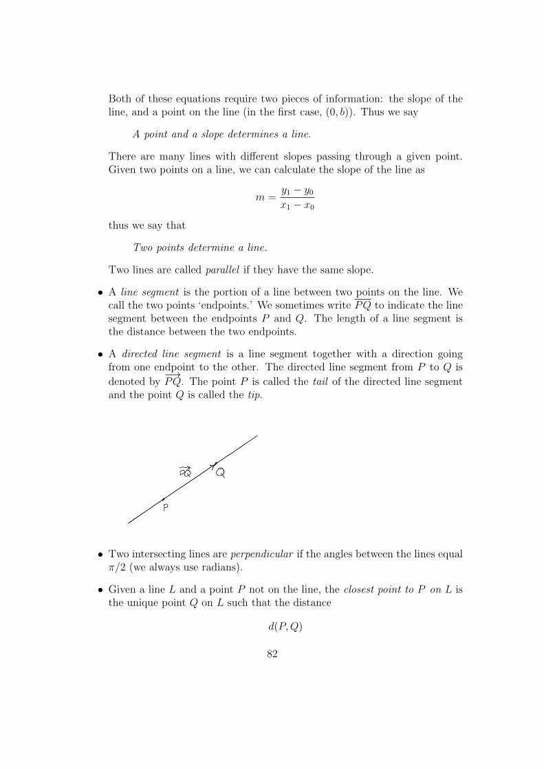
Both of these equations require two pieces of information: the slope of theline, and a point on the line (in the first case, (0, b)). Thus we say
A point and a slope determines a line.
There are many lines with different slopes passing through a given point.Given two points on a line, we can calculate the slope of the line as
m =y1 − y0x1 − x0
thus we say that
Two points determine a line.
Two lines are called parallel if they have the same slope.
• A line segment is the portion of a line between two points on the line. Wecall the two points ‘endpoints.’ We sometimes write PQ to indicate the linesegment between the endpoints P and Q. The length of a line segment isthe distance between the two endpoints.
• A directed line segment is a line segment together with a direction goingfrom one endpoint to the other. The directed line segment from P to Q is
denoted by−→PQ. The point P is called the tail of the directed line segment
and the point Q is called the tip.
• Two intersecting lines are perpendicular if the angles between the lines equalπ/2 (we always use radians).
• Given a line L and a point P not on the line, the closest point to P on L isthe unique point Q on L such that the distance
d(P,Q)
82

is as small as possible. It is a geometric fact that this point, Q, can be con-structed as the intersection of L and the line through P that is perpendicularto L.
• Three points (that don’t line on a line) determine a triangle and these pointsare the vertices of the triangle. Every triangle has three vertices, three sides,and three interior angles. The sum of the three interior angles is always equalto π.
• The law of cosines says that for any triangle as labelled above,
c2 = a2 + b2 − 2ab cos(γ)
• A triangle is a right triangle if one of the interior angles γ = π/2. Righttriangles satisfy the Pythagorean theorem:
a2 + b2 = c2.
• The area of a triangle is computed using the formula
area =base× height
2
83

where base and height are the lengths of line segments indicated in thepicture. In terms of the angle α, the area of the triangle in the picture is
area =base× height
2=ab sin(γ)
2(5.1)
• A parallelogram is a quadrilateral with both pairs of opposite sides parallel.The area of a parallelogram can be computed by dividing it into two trianglesas drawn.
Area = ab sin(γ) (5.2)
5.2 Vectors and points
We have defined Rn to be the set of all n-tuples of real numbers,
Rn = {(x1, . . . , xn) : x1, . . . , xn ∈ R} .
A point in Rn is just a more picturesque way of saying an element of Rn.
84
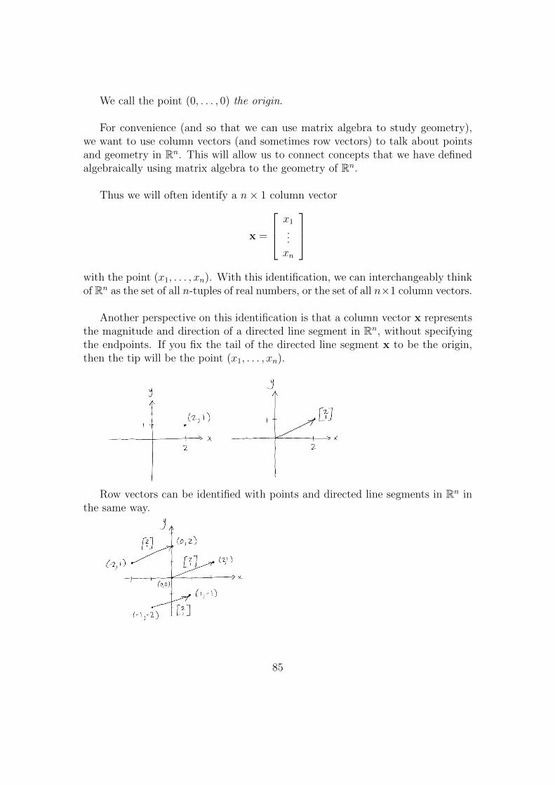
We call the point (0, . . . , 0) the origin.
For convenience (and so that we can use matrix algebra to study geometry),we want to use column vectors (and sometimes row vectors) to talk about pointsand geometry in Rn. This will allow us to connect concepts that we have definedalgebraically using matrix algebra to the geometry of Rn.
Thus we will often identify a n× 1 column vector
x =
x1...xn
with the point (x1, . . . , xn). With this identification, we can interchangeably thinkof Rn as the set of all n-tuples of real numbers, or the set of all n×1 column vectors.
Another perspective on this identification is that a column vector x representsthe magnitude and direction of a directed line segment in Rn, without specifyingthe endpoints. If you fix the tail of the directed line segment x to be the origin,then the tip will be the point (x1, . . . , xn).
Row vectors can be identified with points and directed line segments in Rn inthe same way.
85

5.3 Addition, scalar multiplication, and lines
We can add and scalar multiply points in Rn the same way we add and scalarmultiply column/row vectors.
The sum of two vectors u and v is the vector u + v whose tail is the originand whose tip is the opposite corner of the parallelogram, as drawn.
The difference of two vectors u and v is the vector u − v that can berepresented by the directed line segment whose tail is the tip of v and whosetip is the tip of u.
If P1 = (x1, . . . , xn) is represented by x and P2 = (y1, . . . , yn) is represented byy, then the directed line segment from P1 to P2 can be represented by the vector
y − x =
y1 − x1...
yn − xn
We can use addition of vectors to define lines in Rn.
• Given a point x ∈ Rn and a vector v ∈ Rn, we define the line through xparallel to v to be the set
{x + tv : t ∈ R} .
This is similar to how a point and a slope determined a line in R2.
86

A point and a vector determine a line.
• We can also define a line by specifying two points on the line. If x,y ∈ Rn
are two points, then the line through x parallel to y − x is the set
{x + t(y − x) : t ∈ R} .
Note that this line contains y (set t = 1). Thus, as before,
Two points determine a line.
• A line through the origin parallel to v is the set
{0 + tv : t ∈ R} .
Notice that{0 + tv : t ∈ R} = span {v} .
Thus a line through the origin is the span of a set of one vector.
Definition 5.3. Two non-zero vectors u,v ∈ Rn are parallel if there is a scalar ksuch that u = kv.
Check your understanding
Which of the following vectors are parallel?[1−1
],
[−11
],
[11
]If two vectors u,v ∈ Rn are parallel, then there is a scalar k 6= 0 such that
u = kv. From this we see that
span {u} = span {kv} = span {v}
so two parallel vectors span the same line through the origin.
Equality of sets
Two sets are equal if they contain the same objects.
87

This concept is important because sometimes there are often multiple waysto express a set using set-builder notation (or by other means). Above, we sawthat if u,v ∈ Rn are parallel, then the two sets
span {u} := {tu : t ∈ R}
andspan {v} := {tv : t ∈ R}
are the same, even though the set-builder description of each span looksslightly different.
Here is a similar example. Suppose as before that we are considering setsof shirts that I own. Suppose I own three shirts: my blue Blue Jays shirt (sizemedium), my blue gym shirt (size medium), and my white Honest Ed’s shirt(size large). Consider the following two sets of shirts:
{s ∈ my shirts : s is blue}
and{s ∈ my shirts : the size of s is medium}.
We see that both of these set-builder descriptions describe the same set ofshirts. Thus we write
{s ∈ my shirts : s is blue} = {s ∈ my shirts : the size of s is medium}.
There are several ways to show that two sets are equal. We will see more aboutthis later.
Definition 5.4. Two or more points in Rn are collinear if they lie on the sameline.
Since any two points x and y determine the line
L := {x + t(y − x) : t ∈ R} ,
three points x, y and z are collinear if z is contained in the line L. In other words,x, y and z are collinear if there is a number t ∈ R such that
z = ty + (1− t)x.
88

In-class exercise
For which values of c are the following three points in R3 collinear?
(1,−1), (−1, 1), (0, c)
If P0 = x, P1 = y and P2 = z are collinear, then the vectors−−→P0P1 and
−−→P0P2
are parallel.
Proof. Write If x, y and z are collinear then there is a number t ∈ R such that
z = ty + (1− t)x.
Then −−→P0P1 = y − x
and −−→P0P2 = z− x = ty + (1− t)x− x = t(y − x).
Thus −−→P0P2 = t
−−→P0P1,
so the two vectors are parallel.
In-class exercise
The vectors, [1 2 0 5] and [2 4 0 10] are parallel. What is the rank of thematrix [
1 2 0 52 4 0 10
]?
More generally, suppose that u = [u1 . . . un], v = [v1 . . . vn] are two parallel,nonzero vectors. What is the rank of the matrix[
u1 · · · unv1 · · · vn
]?
Justify your answer.
5.4 The distance between two points
The definition of distance between two points in R2 generalizes to Rn in a naturalway.
89

Definition 5.5. If P1 = (x1, . . . , xn) and P2 = (y1, . . . , yn) are points in Rn, thenthe distance between the two points is defined as
d(P1, P2) :=√
(y1 − x1)2 + · · ·+ (yn − xn)2.
Definition 5.6. The length or norm of a vector v is defined to be
||v|| :=√v21 + · · ·+ v2n.
Example 5.7. The length of the zero vector is 0:
||0|| =√
02 + · · ·+ 02 = 0.
Check your understanding
Compute the length of the vector 1−12
∈ R3.
Compute the distance between the two points P = (1, 0, 1) and Q =(0, 1,−1).
For any vector x,
(a) If ||x|| = 0, then x = 0.
(b) For any scalar k, ||kx|| = |k| · ||x||.
Recall that if P1 = (x1, . . . , xn) is represented by x and P2 = (y1, . . . , yn) isrepresented by y, then the directed line segment from P1 to P2 can be representedby the vector
y − x =
y1 − x1...
yn − xn
and we see that
d(P1, P2) =√
(y1 − x1)2 + · · ·+ (yn − xn)2 = ||y − x||.
90

In R2, the unit circle is the set of all points that are distance 1 from the origin.If we view points as vectors, then it is the set of all vectors with norm = 1.
Definition 5.8. A vector x is called a unit vector if ||x|| = 1.
In-class exercise
Which of the following vectors in R3 are unit vectors? 1−12
, 0−10
, 1/
√2
−1/√
20
, sin(α)
0cos(α)
.
5.5 The dot product
Definition 5.9. The dot product of two vectors u,v ∈ Rn is the scalar
u · v := u1v1 + · · ·+ unvn.
Example 5.10. 1−12
· 0−10
= (1)(0) + (−1)(−1) + (2)(0) = 1.
Matrix multiplication gives us another way to write a dot product:
uTv = [u1 · · ·un]
v1...vn
= u1v1 + · · ·+ unvn = u · v.
91

There is a simple relationship between the dot product of a vector with itselfand its norm,
||u||2 =
(√u21 + · · ·+ u2n
)2
= u21 + · · ·+ u2n = u · u.
Properties of the dot-product:
For any vectors u,v,w ∈ Rn.
(a) u · v = v · u
(b) u · (v + w) = u · v + u ·w
(c) (ku) · v = k(u · v) = u · (kv).
For any two vectors, we see that
||u + v||2 = (u + v) · (u + v) = ||u||2 + 2(u · v) + ||v||2.
This is a useful formula for computation.
In-class exercise
Suppose u,v ∈ Rn such that ||u|| = 2, ||v|| = 1, and ||u + v|| = 1. What isu · v?
Theorem 5.11 (The Cauchy-Schwartz inequality). For any two vectors u,v ∈ Rn,
|u · v| ≤ ||u||||v||.
We can use this to prove the triangle inequality:
Theorem 5.12 (The triangle inequality). For any two vectors u,v ∈ Rn,
||u + v|| ≤ ||u||+ ||v||.
Proof. Let’s start with the square of the left hand side and show it is less than orequal to the square of the right hand side.
92

||u + v||2 = (u + v) · (u + v)
= ||u||2 + 2(u · v) + ||v||2
≤ ||u||2 + 2|u · v|+ ||v||2
≤ ||u||2 + 2||u||||v||+ ||v||2
= (||u||+ ||v||)2.
Thus ||u + v|| ≤ ||u||+ ||v||.
5.6 The angle between two vectors
As in R2, two non-zero vectors u,v ∈ Rn determine two angles: one less than orequal to π and the other larger than or equal to π. The angle between u and v isthe angle that is ≤ π.
Applying the law of cosines to the triangle with sides u,v,u− v, we see that
||u− v||2 = ||u||2 + ||v||2 − 2||u||||v|| cos(θ)
Since||u− v||2 = (u− v) · (u− v) = ||u||2 − 2(u · v) + ||v||2
we see that(u · v) = ||u||||v|| cos(θ).
Since u,v are non-zero, we may divide both sides to get the formula
u · v||u||||v||
= cos(θ).
If the angle θ = π (in other words, the angle is a right angle), then cos(θ) = 0so the formula tells us that u · v = 0.
Definition 5.13. Two vectors u,v ∈ Rn are orthogonal if
u · v = 0.
Being “orthogonal” is the Rn analogue of two vectors being perpendicular inR2.
Problem 3. Show that two vectors u and v are orthogonal if and only if
||u + v||2 = ||u||2 + ||v||2.
93

Solution. From the equation
||u + v||2 = (u + v) · (u + v) = ||u||2 + 2(u · v) + ||v||2
we see that the equation
||u + v||2 = ||u||2 + ||v||2
is equivalent to the equationu · v = 0.
5.7 Orthogonal projection
The problem of orthogonal projection: Consider the following problem.Given a vector v and a nonzero vector u, we want to be able to write v = v1 + v2
where v1 is parallel to u and v2 is orthogonal to u.
Solution: Since v1 is parallel to u, v1 = ku for some k ∈ R, so we have
v = ku + v2
Taking the dot product of both sides of this equation with u, we get
u · v = u · (ku + v2) = k||u||2
(question: why is the equality on the right hand side true?). This equation can besolved for k, which gives us the solution for v1.
v1 = ku =u · v||u||2
u.
Knowing v1, we can then solve for v2,
v2 = v − v1 = v − u · v||u||2
u.
Thus we have found v1 and v2 that solve the problem above.
Check your understanding
At the beginning of the section we said that u was a nonzero vector. Wheredid we use this assumption in our solution to the problem of orthogonalprojection?
94

In fact, the vectors v1 and v2 solving the problem of orthogonal projectionare unique (it is worth trying to check this for yourself). These vectors are quiteimportant in linear algebra, so we give them names.
The orthogonal projection of v onto the line through the origin spanned byu is given by the formula
proju(v) =u · v||u||2
u.
The projection of v orthogonal to the line spanned by u is the vector
v − proju(v).
In-class exercise
In general, what is the angle between u and v− proju(v)? Can you write aproof?
Hint: use the material from the previous two sections.
Recall that the distance between a point P and a line L is defined as theshortest distance between P and any point on L. The following theorem tells usthat given a line and a point, the shortest line segment between the point and theline is given by the projection orthogonal to the line.
Theorem 5.14. The distance between the line through the origin spanned by uand the point represented by the vector v equals the length of v − proju(v) (theprojection of v orthogonal to the line spanned by u).
Proof. We know that proju(v) is a point on the line spanned by u. Using theformula for distance, we compute
d (v, proju(v)) = ||v − proju(v)||.
95

In order to show that this is the distance between v and the line spanned by u, itremains to explain why for any other point Q′ = ku on this line,
d (v, proju(v)) ≤ d(v, Q′).
This final step is left an exercise (hint: use pythagoras and the result of the in-classexercise above).
5.8 Planes in R3
In R2, a linear equation y = mx+b determines a line with slope m and y-interceptb. In R3, a single linear equation determines a plane.
Definition 5.15. A set of points in R3 defined by a single linear equation,
a1x+ a2y + a3z = b
is called a plane.
Example 5.16. (a) The equation x = 0 defines the yz-plane
{(x, y, z) ∈ R3 : x = 0} = {(0, y, z) ∈ R3 : y, z ∈ R}.
(b) The equation y = 0 defines the xz-plane
{(x, y, z) ∈ R3 : y = 0} = {(x, 0, z) ∈ R3 : x, z ∈ R}.
(c) The equation x = 1 defines the
{(x, y, z) ∈ R3 : x = 1} = {(1, y, z) ∈ R3 : y, z ∈ R}.
Given three distinct points, P0, P1, P2 not collinear (not lying on a line), thereis a unique equation
a1x+ a2y + a3z = b
such that P0, P1, P2 are all solutions to the equation. Thus we say,
Three non-collinear points determine a plane.
96

Example 5.17. Find the equation of the plane that contains the three pointsP0 = (1, 1, 0), P1 = (1, 0, 1) and P2 = (0, 0, 1).
We want to find coefficients a1, a2, a3 and b so that all three points are solutionsof the equation
a1x+ a2y + a3z = b.
This problem is a linear system of equations, where the variables are a1, a2, a3and the coefficients come from the points P0, P1, P2!
a1 + a2 = b
a1 + a3 = b
a3 = b
The augmented matrix of this system is 1 1 0 b1 0 1 b0 0 1 b
−→ 1 1 0 b
0 −1 1 00 0 1 b
Back substituting gives a3 = b, a2 = a3 = b, and a1 = b − a2 = 0. Thus (takingb = 1), the equation of the plane is
y + z = 1.
Given a vector a = [a1 a2 a3]T , the plane determined by the equation
a1x+ a2y + a3z = b
is the same as the set
{[x, y, z]T ∈ R3 : a · [x, y, z]T = b}
The vector a is called a normal vector to the plane. Since the plane is determinedby a and b we say
A normal vector and a number determine a plane.
Definition 5.18. Two planes are called parallel if their normal vectors are parallel.
Example 5.19. The two planes
2x+ 4y + z = 0
and−4x− 8y − 2z = 5
are parallel.
97

If a plane is defined by a homogeneous equation,
a1x+ a2y + a3z = 0
then the point (0, 0, 0) lies in the plane. We say that the plane contains the origin.
Definition 5.20. The cross-product of two vectors u,v ∈ R3 is the vector u× vdefined by the formula u1
u2u3
× v1v2v3
:=
u2v3 − u3v2u3v1 − u1v3u1v2 − u2v1
.The cross-product has three beautiful geometric properties.
Geometric properties of the cross-product:
(a) u× v is orthogonal to u and v.
(b) If u and v are parallel, then u× v = 0.
(c) ||u × v|| =√||u||2||v||2 − (u · v)2 = ||u||||v|| sin(θ), where 0 ≤ θ ≤ π is
the angle between u and v.
Note that the right hand side is the formula for the area of the parallelogramwith adjacent sides u and v.
98

Proof. The proofs of these properties are straightforward applications of the defi-nition. For instance, to prove (a), we simply compute
(u× v) · u =
u2v3 − u3v2u3v1 − u1v3u1v2 − u2v1
· u1u2u3
= u1(u2v3 − u3v2) + u2(u3v1 − u1v3) + u3(u1v2 − u2v1)= 0.
Since the dot product is 0, the two vectors are orthogonal. The same works toshow (u× v) · v = 0.
We can use the cross-product to solve the example above a different way.
Example 5.21. Find the equation of the plane that contains the three pointsP0 = (1, 1, 0), P1 = (1, 0, 1) and P2 = (0, 0, 1).
First, we compute the vectors
−−→P0P1 = (0,−1, 1)
−−→P0P2 = (−1,−1, 1)
Then we compute the cross-product,
−−→P0P1 ×
−−→P0P2 =
(−1)(1)− (1)(−1)0− 1(−1)
0− (−1)(−1)
=
0−1−1
.We claim that
−−→P0P1×
−−→P0P2 is the normal vector to the plane that contains P0, P1, P2.
Indeed, we can check that the three points satisfy the equation
0x− y − z = −1.
Check your understanding
In examples 5.17 and 5.21 we found the equation of the plane containingthe points P0 = (1, 1, 0), P1 = (1, 0, 1) and P2 = (0, 0, 1) two different ways.
Even though the two equations we found look slightly different, they describethe same plane. Why?
99
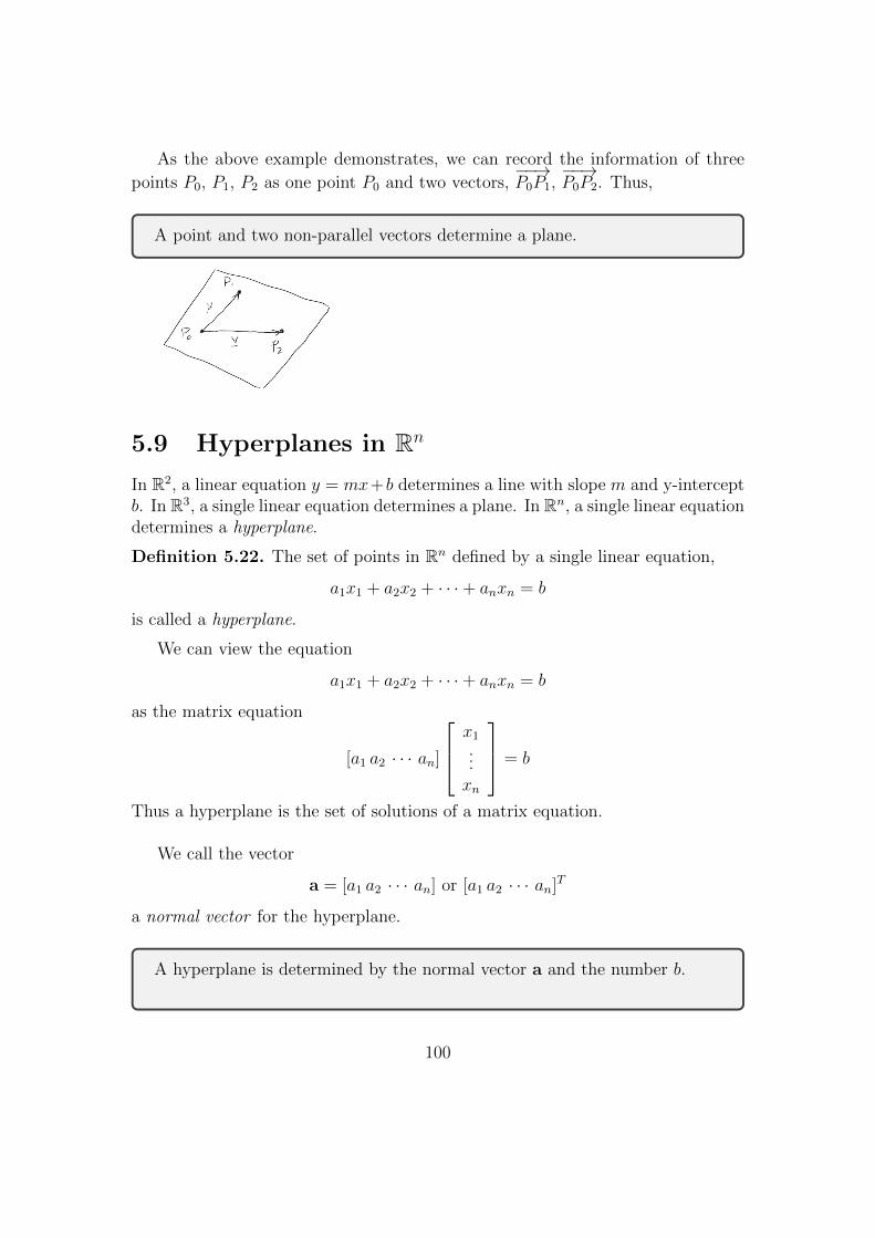
As the above example demonstrates, we can record the information of three
points P0, P1, P2 as one point P0 and two vectors,−−→P0P1,
−−→P0P2. Thus,
A point and two non-parallel vectors determine a plane.
5.9 Hyperplanes in Rn
In R2, a linear equation y = mx+b determines a line with slope m and y-interceptb. In R3, a single linear equation determines a plane. In Rn, a single linear equationdetermines a hyperplane.
Definition 5.22. The set of points in Rn defined by a single linear equation,
a1x1 + a2x2 + · · ·+ anxn = b
is called a hyperplane.
We can view the equation
a1x1 + a2x2 + · · ·+ anxn = b
as the matrix equation
[a1 a2 · · · an]
x1...xn
= b
Thus a hyperplane is the set of solutions of a matrix equation.
We call the vector
a = [a1 a2 · · · an] or [a1 a2 · · · an]T
a normal vector for the hyperplane.
A hyperplane is determined by the normal vector a and the number b.
100

5.10 Application: binary classifiers in R2
Suppose we are perform a series of experiments where we add different quantitiesof two chemicals (let’s call them A and B) together and observe the colour ofthe mixture. We know that, depending on the amount of the two chemicals, themixture will turn red or blue. The goal of the experiments is to find an equation(depending on the quantities of chemicals added) that will predict the colour ofthe resulting mixture. Such an equation can be called a “binary classifier” since itpredicts one of two (binary) experimental outcomes (classes).
We can record our series of experiments as points (xi, yi) ∈ R2. For the ithexperiment, xi is the amount of chemical A in millilitres and yi is the amountof chemical B in millilitres. To each point we also associate the outcome of ourexperiment: whether the mixture was red or blue. We can do this visually bycolouring the points red or blue (see Figure).
This is a nice graphical representation of our experimental data, but we haven’tsolved the problem yet. We want to find an equation that predicts whether themixture will be red or blue. One example of such an equation, would be an equationof a line,
y = mx+ b
(where m and b are coefficients we haven’t determined yet) that divides our datapoints into the two classes of red and blue: e.g. all the red outcomes lie below theline, and all the blue outcomes lie above. In other words, we want that all the reddata points (xi, yi) satisfy
yi ≤ mxi + b
and all the blue data points satisfy
yi ≥ mxi + b
Looking at the figure for this example, we can see that there are several lines thatwill solve our problem. Which one should we pick?
First, we can make the following hypothesis to narrow down the problem: givenwhat we know about mixing chemicals, we reason that it is likely the colour ofthe mixture only depends on the ratio m = x/y of the two chemicals. We havesome evidence for this: the data point on the x axis tells us that if we only addchemical A the mixture is red, and the data point on the y axis tells us that if weonly add chemical B, the mixture is blue. In other words, our line separating thetwo classes should go through the origin (set the coefficient b = 0).
Thus we have reduced our problem to finding a suitable value for m, but again,there are many choices. One reasonable choice is to pick the line that is “furthest”from both sets of points. To quantify furthest, we need to use the notion of distance
101

between a point and a line1. This is the basic idea behind the maximal marginclassifier : for your binary classifier, choose the line that maximizes the distancesto points in both data sets2. See the Figures for an illustration.
This example illustrates a large family of problems in applied mathematicscalled “classification problems.” In classification problems, one has a collectionof data points labelled by classes, and one seeks an equation (or equations) thatwill sort the data points into classes. This type of problem is extremely broad; itcontains everything from the relatively simple example described above, to prob-lems such as detecting cancer from a radiological scan which are at the forefrontof modern research. Some general characteristics of these problems are as follows:
• In general, it may be impossible to find a line that divides the two classes.In this case one might consider variation on the maximal margin classifiercalled the support vector classifier or more general non-linear versions calledsupport vector machines.
• In the example above each data point was a pair of numbers because we hadtwo relevant pieces of information (amount of chemical A and amount ofchemical B). In general classification problems there will be a fixed numbern of relevant quantities and each data point is an n-tuple of numbers. Forinstance, each radiological scan might be a 64 × 64 pixel black and whiteimage, which can be interpreted as a 4096-tuple. By the end of the class,you will have all the tools necessary to understand the maximal marginclassifier for n-dimensional data.
• It is also common that there are more than just two classes.
Hopefully, this application illustrates how geometry of Rn is useful in solving manypractical problems.
5.11 Discussion: geometry of the universe
1A reader might find it useful at this point to go back in the notes and recall the meaning ofthis in terms of orthogonal projections.
2In general, the maximal margin classifier does not have the added constraint that b = 0,which was specific to our example.
102

Key concepts from Chapter 5
The parallelogram rule, definition of a line in Rn, the distance between twopoints, the length of a vector, the dot product, properties of vector lengthand dot product, the Cauchy Schwartz inequality, the triangle inequality, thedefinition of orthogonal vectors, the definition of lines and planes in R3,three non-collinear points determine a plane, a point and two non-parallelvectors determine a plane, the cross-product, properties of the cross-product,definition of a hyperplane in Rn, a point and a normal vector determine ahyperplane.
103
Chapter 6
Linear transformations
In calculus of several variables, one studies real valued functions of several vari-ables, which are functions f : R2 → R, f : R3 → R and so on, and vector fields,which are just functions F : R2 → R2, F : R3 → R3 and so on.
In linear algebra, we are interested in a very special class of functions T : Rn →Rm called linear transformations. The theory of linear transformations is inti-mately connected to vector geometry, the study of systems of linear equations andmatrix algebra.
6.1 Functions from Rn to Rm
Definition 6.1. A function F from Rn to Rm is a rule that assigns a pointF (x) ∈ Rm to every point x ∈ Rn. The set Rn is called the domain of F andthe set Rm is called the codomain of F .
We often use the notation F : Rn → Rm to mean “F is a function from Rn toRm.”
In calculus one often considers functions whose domain is some subset of R. Inthis class we focus on functions whose domain is all of R or all of Rn.
Example 6.2. Here are some examples of functions from Rn to Rm.
(a) A real valued function of one variable, is a function from R1 to R1. Forinstance,
f(x) = sin(x), g(x) = x2, h(x) = 2x+ 1, k(x) = 5x.
104

(b) A real valued function of two variables is a function from R2 to R1. Forinstance,
T (x, y) = x2 + 2xy + 1, S(x, y) = 3x− y.
If we write elements of R2 as vectors, then these functions might be writtenlike this:
T
([xy
])= x2 + 2xy sin(x) + 1, S
([xy
])= 3x− y.
(c) The general form of a function from R3 to R3 is
F (x, y, z) = (F1(x, y, z), F2(x, y, z), F3(x, y, z)) .
Here F1(x, y, z), F2(x, y, z), F3(x, y, z) are real valued functions of three vari-ables. In other words, each FI is a map from R to R3.
For example, here are some functions from R3 to R3.
F (x, y, z) = (1, 0, 0), G(x, y, z) = (x+ y, z − y, x+ 2),
H(x, y, z) = (x− 2y, z − x, y + z + x).
We can also write these functions in vector form:
F
xyz
=
100
, G x
yz
=
x+ yz − yx+ 2
,
H
xyz
=
x− 2yz − x
y + z + x
.Check your understanding
The formulaF (w, x, y, z) = (x+ w, y2)
defines a function. What is the domain and codomain of F?
105

6.2 Linear transformations
In linear algebra, we are primarily interested in a very special kind of functionfrom Rn to Rm called a “linear transformation.”
Definition 6.3. A function T : Rn → Rm is a linear transformation if for allvectors u,v ∈ Rn and for all scalars c ∈ R, both of the following conditions aretrue:
(a) T (u + v) = T (u) + T (v).
(b) T (cu) = cT (u).
It is common to say “T is linear” when one means “T is a linear transforma-tion.”
If T : Rn → Rm is a linear transformation, then T (0) = 0.
Check your understanding
Let u =
[13
]and v =
[1−1
].
Suppose that T : R2 → R2 is a linear transformation such that
T (u) =
[10
]T (v) =
[01
].
What isT (3u + 2v)?
If T : Rn → Rm is a linear transformation, then for all t1, · · · tk ∈ R andu1, . . . ,uk ∈ Rn,
T (c1u1 + · · ·+ ckuk) = c1T (u1) + · · ·+ ckT (uk).
In other words, linear transformations send linear combinations to linearcombinations.
106

In-class exercise
For each of the functions below, defined in Example 6.2, determine whetherthe function is a linear transformation.
•f(x) = sin(x), g(x) = x2, h(x) = 2x+ 1, k(x) = 5x.
•T
([xy
])= x2 + 2xy sin(x) + 1, S
([xy
])= 3x− y.
•F (x, y, z) = (1, 0, 0), G(x, y, z) = (x+ y, z − y, x+ 2),
H(x, y, z) = (x− 2y, z − x, y + z + x).
A function T : Rn → Rm is a linear transformation if for every c ∈ R andu,v ∈ Rn,
T (u + cv) = T (u) + cT (v).
Proof. Suppose that T satisfies T (u+cv) = T (u)+cT (v) for all vectors u,v ∈ Rn
and all scalars c ∈ R. Then, by setting c = 1, since T is linear
T (u + v) = T (u) + T (v)
and by setting u = 0,
T (c0) = cT (v).
Therefore, T is a linear transformation.
6.3 Matrix transformations are linear
Given a m×n matrix A, matrix-vector multiplication defines a map TA : Rn → Rm
by the formulaTA(x) := Ax
where the expression on the right hand side is matrix-vector multiplication. Sinceit is defined using a matrix, we call TA a matrix transformation.
Matrix transformations are linear.
107

Proof. Let u and v be vectors in Rn and let c be a scalar. Then,
TA(u + cv) = A(u + cv) (Defintion of TA)
= Au + A(cv) (Property of matrix multiplication)
= Au + cAv (Property of matrix multiplication)
= TA(u) + cTA(v) (Definition of TA).
Hence, TA(u + cv) = TA(u) + cTA(v). This means that the function TA is a lineartransformation.
6.4 Transformations of R2
Example 6.4. Rotation around a point by θ degrees is a linear transfor-mation
F (x, y) = (cos(θ)x− sin(θ)y, sin(θ)x+ cos(θ)y).
Example 6.5. Translation is not a linear transformation. If (a, b) ∈ R2,translation by (a, b) is the function
F (x, y) = (x, y) + (a, b) = (x+ a, y + b).
Example 6.6. Scaling is a linear transformation. Given k ∈ R, we can definethe function
F (x, y) = (kx, ky).
108

Example 6.7. Scaling in one coordinate is a linear transformation.
F (x, y) = (kx, y).
Example 6.8. Shear transformation is a linear transformation.
F (x, y) = (x+ ay, y).
Example 6.9. Projection to a line through the origin is a linear transfor-mation.
109

Example 6.10. Reflection around a line through the origin is a lineartransformation. Reflection through the y-axis:
F (x, y) = (−x, y).
Reflection through the x-axis:
F (x, y) = (x,−y).
Reflection through the line y = x:
F (x, y) = (y, x).
Reflection through the line y = −x:
F (x, y) = (−y,−x).
Example 6.11. Reflection through the origin is a linear transformation.Reflection through the origin:
F (x, y) = (−x,−y).
110

6.5 The matrix of a linear transformation
In-class exercise
We showed that the function
H
xyz
=
x− 2yz − x
y + z + x
is a linear transformation. Find a 3× 3 matrix A so that
A
xyz
=
x− 2yz − x
y + z + x
.In other words, find a matrix A so that H = TA.
In general, if T : Rn → Rm is a linear transformation, we can always find am× n matrix A so that T = TA. Since any vector in Rn,
x1x2...xn
= x1e1 + x2e2 + · · ·+ xnen,
we know that since T is a linear transformation,
T
x1x2...xn
= x1T (e1) + x2T (e2) + · · ·+ xnT (en) .
111
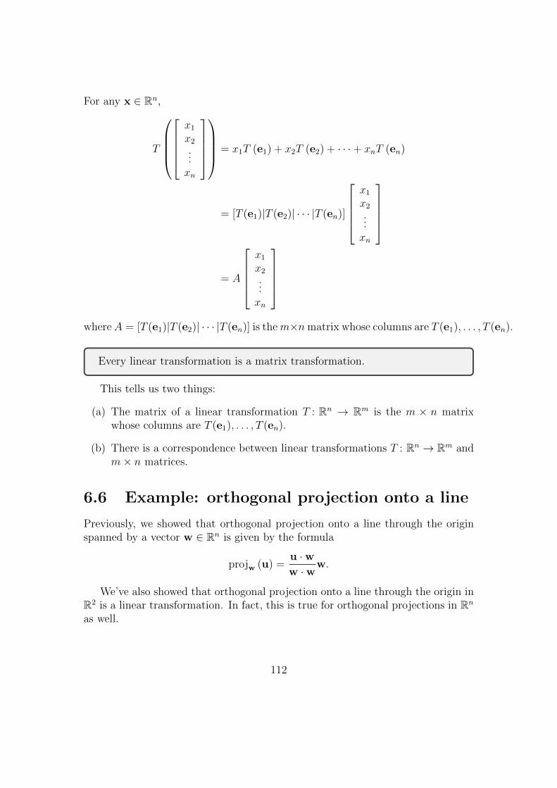
For any x ∈ Rn,
T
x1x2...xn
= x1T (e1) + x2T (e2) + · · ·+ xnT (en)
= [T (e1)|T (e2)| · · · |T (en)]
x1x2...xn
= A
x1x2...xn
whereA = [T (e1)|T (e2)| · · · |T (en)] is them×nmatrix whose columns are T (e1), . . . , T (en).
Every linear transformation is a matrix transformation.
This tells us two things:
(a) The matrix of a linear transformation T : Rn → Rm is the m × n matrixwhose columns are T (e1), . . . , T (en).
(b) There is a correspondence between linear transformations T : Rn → Rm andm× n matrices.
6.6 Example: orthogonal projection onto a line
Previously, we showed that orthogonal projection onto a line through the originspanned by a vector w ∈ Rn is given by the formula
projw (u) =u ·ww ·w
w.
We’ve also showed that orthogonal projection onto a line through the origin inR2 is a linear transformation. In fact, this is true for orthogonal projections in Rn
as well.
112
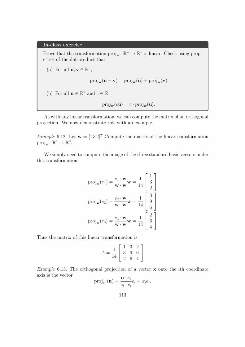
In-class exercise
Prove that the transformation projw : Rn → Rn is linear. Check using prop-erties of the dot-product that:
(a) For all u,v ∈ Rn,
projw(u + v) = projw(u) + projw(v)
(b) For all u ∈ Rn and c ∈ R,
projw(cu) = c · projw(u).
As with any linear transformation, we can compute the matrix of an orthogonalprojection. We now demonstrate this with an example.
Example 6.12. Let w = [1 3 2]T Compute the matrix of the linear transformationprojw : R3 → R3.
We simply need to compute the image of the three standard basis vectors underthis transformation.
projw(e1) =e1 ·ww ·w
w =1
14
132
projw(e2) =
e2 ·ww ·w
w =1
14
396
projw(e3) =
e3 ·ww ·w
w =1
14
264
Thus the matrix of this linear transformation is
A =1
14
1 3 23 9 62 6 4
Example 6.13. The orthogonal projection of a vector x onto the ith coordinateaxis is the vector
projei (u) =u · eiei · ei
ei = xiei.
113

The matrix of this projection is the n×n matrix, all of whose entries are 0, exceptaii = 1.
6.7 Composition of linear transformations
If f : Rn → Rm and g : Rm → Rp are functions, then the composition of g with fis the function g ◦ f : Rn → Rp defined by the formula
g ◦ f(x) := g(f(x)).
As always, brackets are important! The expression on the right hand side means“first apply the function f to the vector x to get f(x), then apply the function gto the vector f(x).”
Example 6.14. For example, consider the functions f, g : R→ R defined by f(x) =x2 + 2, and g(x) = x2. Then
g ◦ f(x) = g(f(x)) = g(x2 + 1) = (x2 + 1)2 = x4 + 2x2 + 1
andf ◦ g(x) = f(g(x)) = f(x2) = (x2)2 + 1 = x4 + 1.
Warning
The composition g ◦ f is only defined if the codomain of f and the domainof g are the same. For instance, if f : R → R2 and g : R → R, then thecomposition
f ◦ g
is defined, but the composition
g ◦ f
is not defined.
If A is a m× n matrix and B is a p×m matrix, then by properties of matrixalgebra, and the definition of composition of functions,
TB ◦ TA(x) = B(Ax) = (BA)x = TBA(x)
Thus we see that
114

If A is a m× n matrix and B is a p×m matrix, then
TB ◦ TA = TBA
This tells us two things:
(a) Composition of linear transformations corresponds to matrix multiplication!
(b) Since TBA is a matrix transformation, and matrix transformations are linear,we know that:
The composition of two linear transformations is a linear transformation.
Warning
If T : Rn → Rn and S : Rn → Rn, then we can define the compositions T ◦Sand S ◦ T , but in general
T ◦ S 6= S ◦ T.
Check your understanding
Can you think of two linear transformations T and S where T ◦ S 6= S ◦ T?
6.8 Kernel and image
There are two important sets associated to every linear transformation.
Definition 6.15. The kernel of a linear transformation T : Rn → Rm is the set
ker(T ) := {x ∈ Rn : T (x) = 0} .
The image of a linear transformation T : Rn → Rm is the set
im(T ) := {T (x) ∈ Rm : x ∈ Rn} .
Note that the kernel of a linear transformation is a set of vectors in the domain,Rn, whereas the image is a set of vectors in the codomain, Rm.
115

SinceTA(x) = Ax
we see that the setker(TA) = {x ∈ Rn : Ax = 0}
which is exactly the set of solutions of the system of linear equations Ax = 0.
Similarly, saying there exists x ∈ Rn such that TA(x) = b is the same assaying that the system of linear equations
Ax = b
is consistent. Equivalently, b is contained in the span of the columns of A.
Problem 4. Let T : R3 → R3 be given by
T (x) =
x1 + x2 + x3x2 + 2x3−x1 + x3
.Write the kernel of T as the span of a set of vectors.
Solution. The matrix of T is
A =
1 1 10 1 2−1 0 1
Thus, we want to write the solution set of Ax = 0 as the span of a set of vectors.We know that the set of solutions to Ax = 0 is the span of the set of basic solutions,so we just need to compute the basic solutions. First, row reducing, 1 1 1
0 1 2−1 0 1
→ · · · →1 0 −1
0 1 20 0 0
.Therefore, there is one basic solution, and the solution set is
ker(T ) = span
1−21
.
116

Problem 5. Let T : R3 → R3 be given by
T (x) =
x1 + x2 + x3x2 + 2x3−x1 + x3
.Write the image of T as the span of a set of vectors.
Solution. We have computed the matrix A of T above. The image of T is the set
im(T ) = {b ∈ R3 : Ax = b is consistent}
Since Ax = b is consistent if and only if b is contained in the span of the columnsof A, we see that
im(T ) = span
1
0−1
, 1
10
, 1
21
.
Definition 6.16. A linear transformation T : Rn → Rm is called injective (orone-to-one) if
ker(T ) = {0} .A linear transformation T : Rn → Rm is called surjective (or onto) if
im(T ) = Rm.
The terminology of “injective” and “surjective” for linear transformations comesfrom a more general definition for maps (linear or not). Since we are only concernedwith linear transformations, the definition above is sufficient for the purposes ofthis course.
• TA is injective if and only if Ax = 0 has only the trivial solution.
• TA is surjective if and only if for every b, the system Ax = b isconsistent.
Example 6.17. The transformation T from the problems above is not injectivesince ker(T ) 6= {0}. It is also not surjective: since the rank of A is 2, by The-orem 6.25, the system Ax = b is not consistent for every b ∈ R3, thus im(T ) 6= R3.
117

Example 6.18. Rotation by θ degrees in R2 is injective and surjective. Indeed, forany value of θ, the matrix of the linear transformation is
A =
[cos(θ) − sin(θ)sin(θ) cos(θ)
].
The quantity ad − bc = cos2(θ) + sin2(θ) = 1, so A is invertible (see Chapter 4).By the big theorem for square matrices, since A is invertible, system Ax = 0 hasonly the trivial solution, so TA is injective.
Similarly, by the big theorem for square matrices, since A is invertible, for ev-ery b ∈ R2, the system Ax = b is consistent, so TA is surjective.
Example 6.19. Let
A =
1 00 11 −1
, and B =
[1 0 00 1 0
].
The linear transformation TA : R2 → R3 is injective but not surjective.
The linear transformation TB : R3 → R2 is surjective but not injective.
Since BA = I2, the composition TB ◦ TA = TBA = TI2 : R2 → R2 is both injec-tive and surjective.
The composition TA ◦ TB = TAB : R3 → R3 is neither injective nor surjective,since
AB =
1 00 11 −1
[ 1 0 00 1 0
]=
1 0 00 1 00 0 0
,so
ker(TAB) =
0
0z
: z ∈ R
6= {0}and
im(TAB) =
xy0
: x, y ∈ R
6= R3.
In-class exercise
Let w = [1 3 2]T .What is the image and kernel of projw?
118

6.9 Invertible linear transformations
Definition 6.20. A function f : Rn → Rm is invertible if there is a map g : Rm →Rn such that
• For all x ∈ Rn, g(f(x)) = x, and
• For all x ∈ Rm, f(g(x)) = x.
The map g is called the inverse of f and sometimes denoted by f−1.
Example 6.21. The function f : R→ R defined by f(x) = 5x+ 2 is invertible. Theinverse g : R→ R is defined by g(x) = 1
5(x− 2), since
f(g(x)) = 5
(1
5(x− 2)
)+ 2 = (x− 2) + 2 = x
g(f(x)) =1
5((5x+ 2)− 2) =
1
5(5x) = x.
Warning
We have now used the word “invertible” and the notation “−1” to mean twodifferent things:
• A square matrix A is invertible if there is a matrix B such that AB =BA = I. The matrix B is called the inverse of A and denoted by A−1.
• A function f is invertible if there is a function g such that f ◦ g(y) = yand g ◦ f(x) = x. The function g is called the inverse of f and isdenoted by f−1.
These two statements look very similar, and the next example shows thatfor linear transformations they are intimately related. But the meaning isdifferent!
Theorem 6.22. The following two statements are equivalent:
(a) The linear transformation T : Rn → Rn is invertible (as a function).
(b) the n× n matrix A of the linear transformation is invertible (as a matrix).
Warning
If n 6= m, then a linear transformation T : Rn → Rm cannot ever be invert-ible. We will see why later in the course.
119
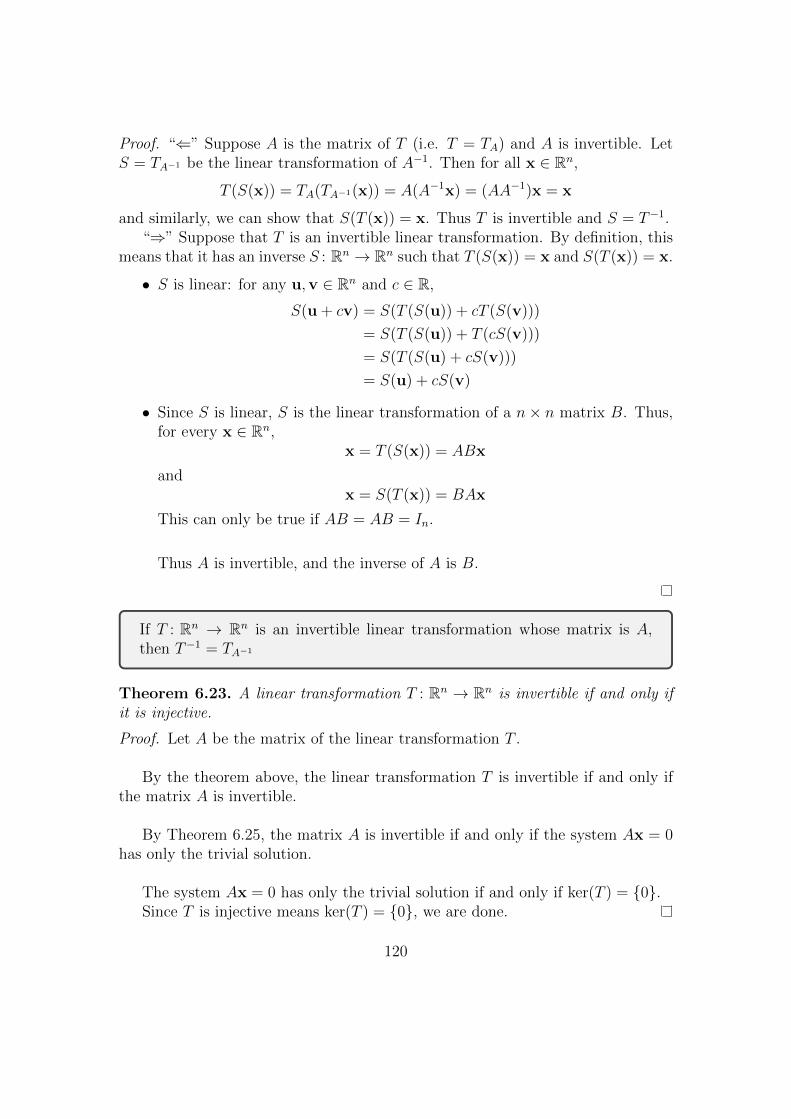
Proof. “⇐” Suppose A is the matrix of T (i.e. T = TA) and A is invertible. LetS = TA−1 be the linear transformation of A−1. Then for all x ∈ Rn,
T (S(x)) = TA(TA−1(x)) = A(A−1x) = (AA−1)x = x
and similarly, we can show that S(T (x)) = x. Thus T is invertible and S = T−1.“⇒” Suppose that T is an invertible linear transformation. By definition, this
means that it has an inverse S : Rn → Rn such that T (S(x)) = x and S(T (x)) = x.
• S is linear: for any u,v ∈ Rn and c ∈ R,
S(u + cv) = S(T (S(u)) + cT (S(v)))
= S(T (S(u)) + T (cS(v)))
= S(T (S(u) + cS(v)))
= S(u) + cS(v)
• Since S is linear, S is the linear transformation of a n× n matrix B. Thus,for every x ∈ Rn,
x = T (S(x)) = ABx
andx = S(T (x)) = BAx
This can only be true if AB = AB = In.
Thus A is invertible, and the inverse of A is B.
If T : Rn → Rn is an invertible linear transformation whose matrix is A,then T−1 = TA−1
Theorem 6.23. A linear transformation T : Rn → Rn is invertible if and only ifit is injective.
Proof. Let A be the matrix of the linear transformation T .
By the theorem above, the linear transformation T is invertible if and only ifthe matrix A is invertible.
By Theorem 6.25, the matrix A is invertible if and only if the system Ax = 0has only the trivial solution.
The system Ax = 0 has only the trivial solution if and only if ker(T ) = {0}.Since T is injective means ker(T ) = {0}, we are done.
120
Theorem 6.24. A linear transformation T : Rn → Rn is invertible if and only ifit is surjective.
Proof. Let A be the matrix of the linear transformation T .
By the theorem above, the linear transformation T is invertible if and only ifthe matrix A is invertible.
By Theorem 6.25, the matrix A is invertible if and only if for every b ∈ Rn,the system Ax = b is consistent.
For every b ∈ Rn, the system Ax = b is consistent if and only if im(T ) = Rn.Since T is surjective means im(T ) = Rn, we are done.
We can summarize these results by adding three more items to the list ofequivalent statements for square matrices:
Theorem 6.25. [The big theorem for square matrices, part 2] Suppose A is a n×nmatrix. The following statements are equivalent:
(a) The matrix A is invertible.
(b) The matrix equation Ax = b has exactly one solution for all n × 1 columnvectors b.
(c) The homogeneous matrix equation Ax = 0 has exactly one solution (thetrivial solution).
(d) The rank of A is n.
(e) The reduced row-echelon form of A is I.
(f) There exists a n× n matrix B such that AB = I.
(g) There exists a n× n matrix B such that BA = I.
(h) A can be written as a product of elementary matrices.
(i) The linear transformation TA : Rn → Rn is invertible.
(j) The linear transformation TA : Rn → Rn is injective (ker(TA) = {0}).
(k) The linear transformation TA : Rn → Rn is surjective (im(TA) = Rn).
121

6.10 Discussion: solving nonlinear problems by
linear approximation
122

Key concepts from Chapter 6
Functions Rn → Rm, definition of linear transformations, properties of lin-ear transformations, matrix linear transformations, transformations of R2,computing the matrix of a linear transformation, orthogonal projections ontoa line through the origin is a linear transformation, composition of functions,the composition of two linear transformations is a linear transformation,composition of linear transformations corresponds to matrix multiplication,definition of kernel and image of linear transformations, definition of invert-ible functions, the big theorem for square matrices (part 2).
123

Chapter 7
Subspaces, span, and linearindependence
We have already learned about lines and hyperplanes in Rn. We might think ofthese as “straight” or “flat” objects in linear algebra. When n > 3, there is anatural generalization of lines through the origin and hyperplanes through the ori-gin called “subspaces.” Subspaces show up many different ways: in the study ofsystems of linear equations, vector geometry, matrix algebra, and linear transfor-mations.
Once we have defined what a subspace is, we are immediately interested indescribing subspaces in a similar way to how we described lines through the ori-gin (as the span of a vector) and planes in R3 (as the span of two non-parallelvectors). This leads to a natural question: “what is the fewest vectors we needto span a subspace?” and this question naturally leads to the notions of “linearindependence,” “basis” and “dimension.”
7.1 Subspaces
Definition 7.1. A set of points in Rn, S, is called a subspace of Rn if the followingthree conditions are satisfied:
I) (S contains the origin) 0 ∈ S.
II) (S is closed under vector addition) If u,v ∈ S, then u + v ∈ S.
III) (S is closed under scalar multiplication) If u ∈ S and c ∈ R, then cu ∈ S.
124

Check your understanding
Suppose that S is a subspace of R3 that contains the vectors
u =
10−1
, v =
011
.Using the fact that S is a subspace, explain why each of the following vectorsis also contained in S. 0
00
, 0
22
, 1
10
.Example 7.2. Let’s look at some examples.
1. Lines through the origin are subspaces: Given a nonzero vector w ∈ Rn,the line through the origin with direction w is the set
L = {tw ∈ Rn : t ∈ R} = span{w}.
To show L is a subspace of Rn, we check the three conditions:
I) Since 0v = 0, the zero vector is in L.
II) If u,v ∈ L, then u = tw and v = sw for some t, s ∈ R.
Thus, u + v = tw + sw = (t + s)w ∈ L. So L is closed under vectoraddition.
III) If tw ∈ L, then for any c ∈ R, ctw ∈ L. Thus L is closed under scalarmultiplication.
Thus we see that the line L is a subspace of Rn.
2. Lines not through the origin are not subspaces: A line that does notcontain the point 0 fails condition I) of the definition.
3. Planes through the origin in R3 are subspaces: This is true because ofthe next example, which is more general (a hyperplane in R3 is a plane).
4. Hyperplanes through the origin are subspaces: Recall that a hyperplaneH in Rn, containing the origin, is defined by a single homogeneous equation:
H = {x ∈ Rn : a1x1 + a2x2 + · · ·+ anxn = 0} .
To show H is a subspace of Rn, we check the three conditions:
125

I) Since a10 + a20 + · · ·+ an0 = 0, we see that the zero vector is in H.
II) If x,y ∈ H, then
a1(x1 + y1) + a2(x2 + y2) + · · ·+ an(xn + yn) = a1x1 + a2x2 + · · ·+ anxn
+ a1y1 + a2y2 + · · ·+ anyn
= 0 + 0 = 0.
Thus, x + y ∈ H. So H is closed under vector addition.
III) If x ∈ H, then for any c ∈ R,
a1(cx1) + a2(cx2) + · · ·+ an(cxn) = c(a1x1 + a2x2 + · · ·+ anxn)
= c(0) = 0
Thus cx ∈ H.
Thus we see that the hyperplane H is a subspace of Rn.
5. The circle in R2 centred at (1, 0) with radius 1 is not a subspace: Thecircle in R2 centred at (1, 0) with radius 1 is the set of vectors
S =
{[xy
]∈ R2 :
√(x− 1)2 + y2 = 1
}Let’s see if this set satisfies the conditions for being a subspace.
I) S satisfies this condition.
II) S does not satisfy this condition. The points (1, 1) and (2, 0) are containedin S but (1, 1) + (2, 0) = (3, 1) is not contained in S.
III) S does not satisfy this condition. The point (2, 0) is contained in S butthe point 2 · (2, 0) = (4, 0) is not.
6. The set Rn itself a subspace of Rn. There is almost nothing to check:
I) 0 ∈ Rn.
II) The sum of two vectors in Rn is a vector in Rn.
III) Scalar multiples of a vector in Rn is a vector in Rn.
In-class exercise
Is the set S = {(0, . . . , 0)} a subspace of Rn? Check the three conditions.
126
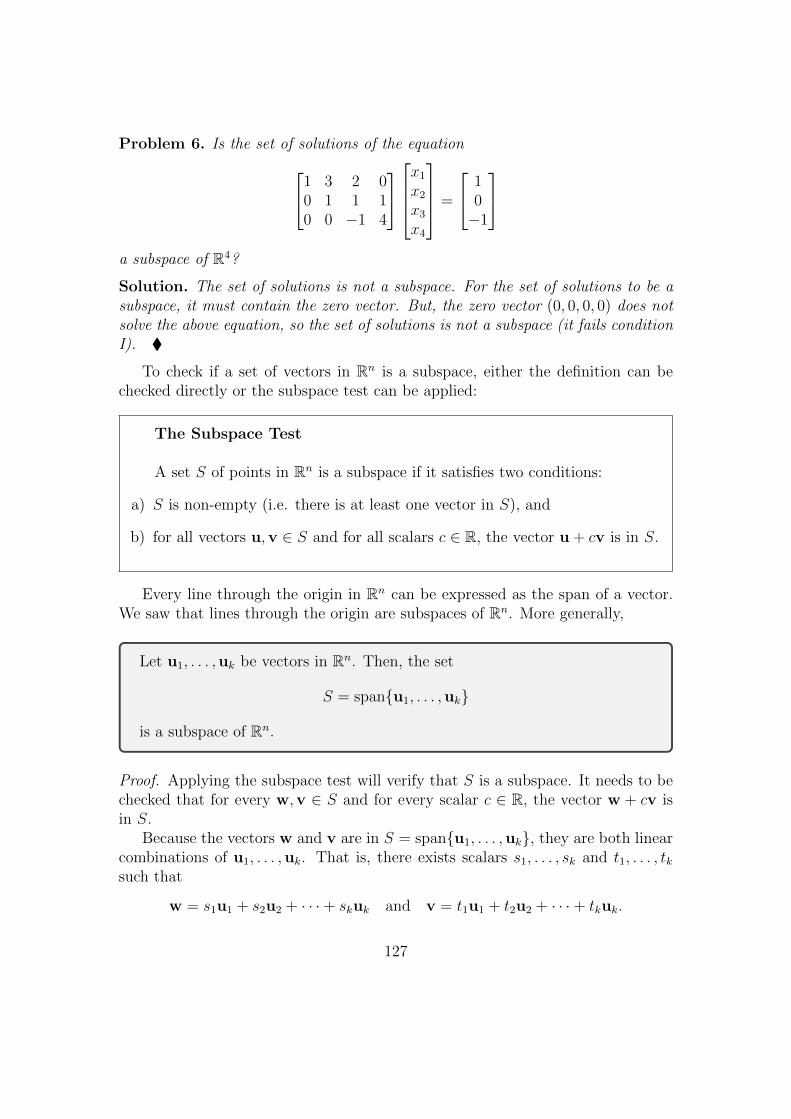
Problem 6. Is the set of solutions of the equation1 3 2 00 1 1 10 0 −1 4
x1x2x3x4
=
10−1
a subspace of R4?
Solution. The set of solutions is not a subspace. For the set of solutions to be asubspace, it must contain the zero vector. But, the zero vector (0, 0, 0, 0) does notsolve the above equation, so the set of solutions is not a subspace (it fails conditionI). �
To check if a set of vectors in Rn is a subspace, either the definition can bechecked directly or the subspace test can be applied:
The Subspace Test
A set S of points in Rn is a subspace if it satisfies two conditions:
a) S is non-empty (i.e. there is at least one vector in S), and
b) for all vectors u,v ∈ S and for all scalars c ∈ R, the vector u + cv is in S.
Every line through the origin in Rn can be expressed as the span of a vector.We saw that lines through the origin are subspaces of Rn. More generally,
Let u1, . . . ,uk be vectors in Rn. Then, the set
S = span{u1, . . . ,uk}
is a subspace of Rn.
Proof. Applying the subspace test will verify that S is a subspace. It needs to bechecked that for every w,v ∈ S and for every scalar c ∈ R, the vector w + cv isin S.
Because the vectors w and v are in S = span{u1, . . . ,uk}, they are both linearcombinations of u1, . . . ,uk. That is, there exists scalars s1, . . . , sk and t1, . . . , tksuch that
w = s1u1 + s2u2 + · · ·+ skuk and v = t1u1 + t2u2 + · · ·+ tkuk.
127

Thus,
w + cv = (s1u1 + s2u2 + · · ·+ skuk) + (t1u1 + t2u2 + · · ·+ tkuk)
= (s1 + ct1)u1 + (s2 + ct2)u2 + · · ·+ (sk + ctk)uk.
Since w + cv can be written as a linear combination of the vectors u1, . . . ,uk, wehave shown that
w + cv ∈ span{u1, . . . ,uk} = S.
By the subspace test, we have shown that S is a subspace.
Check your understanding
The set of solutions of a system of linear equations Ax = b is a set ofvectors in Rn.
For which values of b is the set of solutions a subspace of Rn?
7.2 The span of a set of vectors
As we saw in the previous section, the span of a set of vectors in Rn is a subspaceof Rn. There are many different ways to express a subspace as the span of a setof vectors.
Example 7.3. R3 can be written as a span of a set of vectors many different ways.
1. R3 can be written as the span of the set of standard basis vectors,
R3 = span
1
00
,0
10
,0
01
.
Since for any vector in R3,xyz
= x
100
+ y
010
+ z
001
.2. R3 can be written as the span of the set of standard basis vectors along with
any other vectors. For instance,
R3 = span
1
00
,4
00
,0
10
,0
01
, 1
2−4
,3
11
.
128

Since for any vector in R3,xyz
= x
100
+ 0
400
+ y
010
+ z
001
+ 0
12−4
+ 0
311
3. R3 can be written as the span of three vectors many other ways. For instance,
R3 = span
1
0−1
,2
10
,0
21
.
4. Since two vectors in R3 either span the set {0} (if they are both zero), or aline (if they are parallel), or a plane (if they are not parallel), then for any twovectors in R3,
R3 6= span{u,v}.
We need at least 3 vectors to span R3!
Check your understanding
Consider the two spans,
span
1
00
,0
10
,
span
0
00
,1
00
,5
00
,0
10
120
, 1−10
.
Are these two subspaces of R3 the same or different? Can you describe themgeometrically?
Example 7.4. Let’s look at some more examples.
1. Two parallel vectors span the same line: As we saw earlier, if k 6= 0, then
span{kx} = span{x}
On the other hand, if x is nonzero and k = 0, then
span{kx} = {0} 6= span{x}.
129
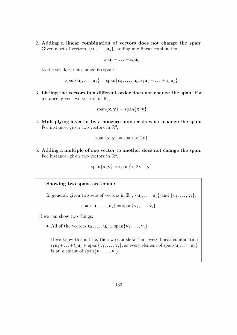
2. Adding a linear combination of vectors does not change the span:Given a set of vectors, {u1, . . . ,uk}, adding any linear combination
s1u1 + . . .+ skuk
to the set does not change its span:
span{u1, . . . ,uk} = span{u1, . . . ,uk, s1u1 + . . .+ skuk}
3. Listing the vectors in a different order does not change the span: Forinstance, given two vectors in R3,
span{x,y} = span{x,y}
4. Multiplying a vector by a nonzero number does not change the span:For instance, given two vectors in R3,
span{x,y} = span{x, 2y}
5. Adding a multiple of one vector to another does not change the span:For instance, given two vectors in R3,
span{x,y} = span{x, 2x + y}
Showing two spans are equal:
In general, given two sets of vectors in Rn, {u1, . . . ,uk} and {v1, . . . ,vi},
span{u1, . . . ,uk} = span{v1, . . . ,vi}
if we can show two things:
• All of the vectors u1, . . . ,uk ∈ span{v1, . . . ,vi}.
If we know this is true, then we can show that every linear combinationt1u1+. . .+tkuk ∈ span{v1, . . . ,vi}, so every element of span{u1, . . . ,uk}is an element of span{v1, . . . ,vi}.
130
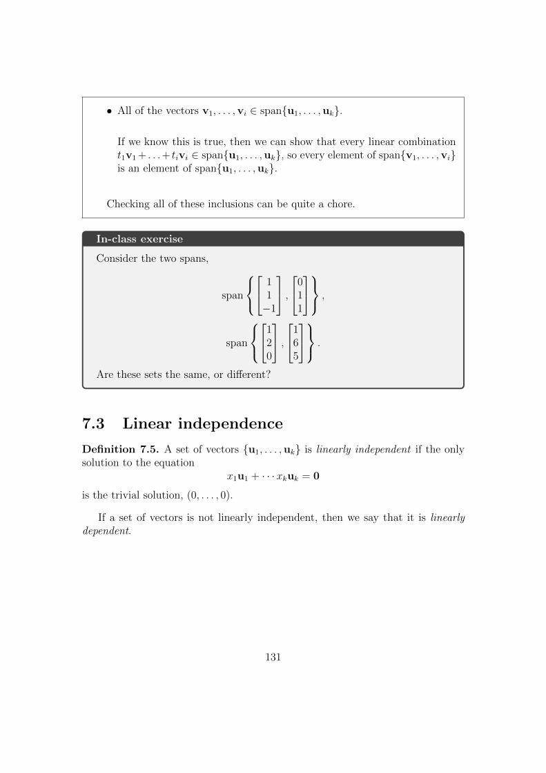
• All of the vectors v1, . . . ,vi ∈ span{u1, . . . ,uk}.
If we know this is true, then we can show that every linear combinationt1v1 + . . .+ tivi ∈ span{u1, . . . ,uk}, so every element of span{v1, . . . ,vi}is an element of span{u1, . . . ,uk}.
Checking all of these inclusions can be quite a chore.
In-class exercise
Consider the two spans,
span
1
1−1
,0
11
,
span
1
20
,1
65
.
Are these sets the same, or different?
7.3 Linear independence
Definition 7.5. A set of vectors {u1, . . . ,uk} is linearly independent if the onlysolution to the equation
x1u1 + · · ·xkuk = 0
is the trivial solution, (0, . . . , 0).
If a set of vectors is not linearly independent, then we say that it is linearlydependent.
131
Check your understanding
Is the set of vectors 1
00
,0
10
linearly independent?
Is the set of vectors0
00
,1
00
,5
00
,0
10
120
, 1−10
linearly independent?
Example 7.6. Let’s look at some examples.
1. A set of one nonzero vector is linearly independent: If u 6= 0, then theonly solution to the equation
xu = 0
is x = 0, so by definition, the set {u} is linearly independent.
On the other hand, the set {0} is linearly dependent, since the equation
x0 = 0
has many solutions (x can be any number).
2. Any set containing 0 is linearly dependent: If a set of vectors {u1, . . . ,uk}contains the vector 0, then it is linearly dependent. Indeed, if uj = 0 for some1 ≤ j ≤ k, then
0u1 + · · ·+ 1uj + · · ·+ 0uk = 0 + · · ·+ 10 + · · ·+ 0 = 0,
so (0, . . . , 1, . . . , 0) is a nontrivial solution to the equation
x1u1 + · · ·+ xkuk = 0,
so the set of vectors is not linearly independent. In other words, it is linearlydependent.
132
3. A set of two nonzero vectors is linearly independent if and only ifthey are not parallel: Suppose we have a set of two nonzero vectors {u,v}in Rn.
If u and v are parallel, then there is a number k such that v = ku. If this istrue, then
(−k)u + v = −v + v = 0
so the set {u,v} is linearly dependent.
On the other hand, if u and v are linearly dependent, then there is a nontrivialsolution (x1, x2) to the equation
x1u + x2v = 0
sou = −x2
x1v
so u and v are parallel.
Warning
In the previous example we explained that for a set of two nonzero vectors{u,v}, the following two statements are equivalent:
(a) {u,v} is linearly independent.
(b) u and v are not parallel.
This doesn’t work so simply for three or more vectors, it is best to usethe definition of linearly independent when you have a set of three or morevectors.
If we view the equation
x1u1 + · · ·xkuk = 0
as the matrix-vector equation
[u1| · · · |uk]
x1...xk
=
0...0
. (7.7)
133

then we see that
The following statements are equivalent:
• The set {u1, . . . ,uk} is linearly independent
• The matrix equation (7.7) has only the trivial solution.
• The matrix [u1| · · · |uk] has rank k.
Determining if a set of vectors is linearly independent:
We know that linear independence of a set of vectors {u1, . . . ,uk} isequivalent to the matrix [u1| · · · |uk] having rank k.
Thus in order to determine if a set of vectors {u1, . . . ,uk} is linearly inde-pendent, we do the following.
1. Write the vectors as columns of a matrix A = [u1| · · · |uk].
2. Use row operations to put the matrix A into REF.
3. From the REF, read off the number of leading entries (rank) of the matrixA.
Once this is done, there are two possibilities:
a. If rank(A) = k (the number of vectors in the set), then the set{u1, . . . ,uk} is linearly independent.
b. If rank(A) < k, then the set {u1, . . . ,uk} is linearly dependent.
134

In-class exercise
The following statement is true:
Every set of more than n vectors in Rn is linearly dependent.
For instance, every set of 4 vectors in R3 is linearly dependent.
Can you explain why?
7.4 Basis
Definition 7.8. Let S be a subspace of Rn. A set of vectors {u1, . . . ,uk} in S isa basis for S if both of the following conditions are satisfied:
I) span{u1, . . . ,uk} = S.
II) The set {u1, . . . ,uk} is linearly independent.
The vectors in a basis are called basis vectors.
Check your understanding
Find a basis for the subspace
span
0
00
,1
00
,5
00
,0
10
120
, 1−10
From our characterizations of span and linear independence in previous sec-
tions, we see that
135

A set of vectors {u1, . . . ,uk} in S is a basis for S if
I) For every b ∈ S, the matrix equation
[u1| · · · |uk]x = b
is consistent.
II) The matrix equation[u1| · · · |uk]x = 0
has exactly one solution.
We can phrase this slightly differently
A set of vectors {u1, . . . ,uk} in S is a basis for S if
I) For every b ∈ S, the matrix equation
[u1| · · · |uk]x = b
is consistent.
II) The matrix [u1| · · · |uk] has rank k (the number of vectors).
Example 7.9. Let’s look at some examples.
1. A basis for a line through the origin: Given a nonzero vector w ∈ Rn, theline through the origin with direction w is the set
L = {tw ∈ Rn : t ∈ R} = span{w}.
Since w 6= 0, the set {w} is linearly independent.
Thus, {w} is a basis for L.
2. A basis for a plane in R3: A plane P in R3 is spanned by two nonparallelvectors u and v. Moreover, two nonparallel vectors are linearly independent.Thus, the set {u,v} is a basis for the plane P = span{u,v}.
3. A basis for the set Rn. We have shown that the standard basis vectorse1, . . . , en span Rn and are linearly independent, so they are a basis for Rn.
136
Let B be a basis for a subspace S. Then, each vector in S can be writtenas a unique linear combination of basis vectors.
Finding a basis for the span of a set of vectors:
Given k vectors u1, . . . ,uk ∈ Rn, we know that S = span{u1, . . . ,uk} is asubspace of Rn.
In order to find a basis for S, we do the following:
1. Write the vectors u1, . . . ,uk as the columns of a n × k matrix A =[u1| . . . |uk].
2. Row-reduce the matrix A until it is in row echelon form R.
3. Identify the columns cj1 , . . . , cjl of the matrix R that contain leading entries.
4. The set of corresponding vectors {uj1 , . . . ,ujl} is a basis for S.
Proof. In order to prove that {uj1 , . . . ,ujl} is a basis for S, we must prove that
• (span) span{uj1 , . . . ,ujl} = S
• (linear independence) {uj1 , . . . ,ujl} is linearly independent.
Span: Since R is in row echelon form, the span of the vectors containing leadingentries cj1 , . . . , cjl equals the span of the set of vectors c1, . . . , ck (see exercisesfrom earlier in the chapter).
Since A → R by elementary row operations, there is an invertible product ofelementary matrices, call it E, so that R = EA. Then A = E−1R. Since
span{cj1 , . . . , cjl} = span{c1, . . . , ck}
it follows that
span{uj1 , . . . ,ujl} = span{E−1cj1 , . . . , E−1cjl}= span{E−1c1, . . . , E
−1ck}= span{u1, . . . ,uk}
137

(see the exercise in the tutorial).
Linear independence: Since R is in row echelon form, the set of vectorscontaining leading entries, {cj1 , . . . , cjl} is linearly independent.
Since E−1 is invertible, it follows that the set of vectors
{uj1 , . . . ,ujl} = {E−1cj1 , . . . , E−1cjl}
is linearly independent (see the tutorial).
In-class exercise
Find a basis for the subspace
span
1
01
,2
02
,1
02
,4
05
7.5 Dimension
Subspaces and bases have the following important property:
Suppose S is a subspace of Rn.
Every basis for S has the same number of vectors.
This allows us to make the following definition.
Definition 7.10. The dimension of a subspace S is the number of vectors in anybasis for S. The dimension of S is denoted dimS.
The dimension of the subspace {0} is 0 by convention.
Example 7.11. Let’s look at some examples.
1. The dimension of a line through the origin is 1: Given a nonzero vectoru, we saw that {u} is a basis for the line L = span{u}. Thus,
dimL = 1.
138

2. The dimension of Rn is n: Since the set of standard basis vectors {e1, . . . , en}is a basis for Rn,
dimRn = n.
3. The dimension of a plane containing the origin in R3 is 2: Since twononparallel vectors are a basis for a plane P = span{u,v} we know that
dimP = 2.
4. The dimension of a hyperplane containing the origin in Rn is n − 1:We will see why this is true in the next chapter.
Theorem 7.12. Let S be a subspace with dimS = k 6= 0. Let U = {u1, . . . ,um}be a set of m vectors in S. Then,
(a) If m < k, then U does not span S.
(b) If m > k, then U is not linearly independent.
(c) If m < k and U is linearly independent, then U can be extended to a basisfor S.
(d) If m > k and U spans S, then U contains a basis for S.
(e) If m = k and U is linearly independent, then U is a basis for S.
(f) If m = k and U spans S, then U is a basis for S.
(g) If S ′ is a subspace of S and dimS ′ = k, then S ′ = S.
7.6 Discussion:
139

Key concepts from Chapter 7
Subspace, span of a set of vectors is a subspace, determining whether twospans are the same, definition of linearly independent, determining whether aset of vectors is linearly independent, definition of a basis, finding a basis forthe span of a set of vectors, dimension of a subspace, facts about dimension.
140
Chapter 8
The fundamental subspaces of amatrix
There are three important subspaces associated to am×nmatrix A: the null space,the column space, and the row space. In this chapter we study these subspaces andhow they are related to each other and the other theories studied in this course.
8.1 The null space of a matrix
Definition 8.1. Let A be an m× n matrix. The null space of A is the set
null(A) := {x ∈ Rn : Ax = 0}.
In other words, the null space of a matrix A is the set of solutions of thehomogeneous system
Ax = 0.
The null space of Am×n is a subspace of Rn.
Proof. Apply the subspace test: Suppose that u,v ∈ S and c ∈ R. u,v ∈ S meansthat both u and v are solutions to the matrix equation Ax = 0.
We need to check that u + cv ∈ S, i.e. the vector u + cv is also a solution toAx = 0. We compute,
A(u + cv) = Au + cAv
= 0 + c0
= 0.
141
Thus, u + cv is also a solution to Ax = 0, so u + cv ∈ S. By the subspace test,we have shown that S is a subspace of Rn.
Example 8.2. Lets look at some examples.
1. The plane through the origin in R3 normal to a vector. If n ∈ R3 is thevector normal to a plane through the origin, P , then
P ={x ∈ R3 : n · x = 0
}If A = [n1 n2 n3], then
null(A) ={x ∈ R3 : Ax = 0
}.
Since Ax = n · x, these two sets are the same:
null(A) = P .
2. Hyperplanes through the origin More generally, if A = [a1 a2 · · · an] is arow vector, then the matrix equation
Ax = 0
is simply the homogeneous equation
a1x1 + a2x2 + · · ·+ anxn = 0.
The set of solutions to this equation is precisely the hyperplane through theorigin,
null(A) = {x ∈ Rn : a1x1 + a2x2 + · · ·+ anxn = 0} .
Thus hyperplanes through the origin are just an example of the null space of amatrix.
3. The line through the origin perpendicular to a plane through theorigin in R3. Recall that a plane through the origin in R3 can be expressed asthe span of two linearly independent vectors u,v ∈ R3:
P = span{u,v}.
The line through the origin in R3 perpendicular to P is the set of all x ∈ R3
that are orthogonal to u and v:
L ={x ∈ R3 : x · u = 0 and x · v = 0
}.
142

If
A =
[u1 u2 u3v1 v2 v3
]then
null(A) ={x ∈ R3 : Ax = 0
}= L.
If A is a m×n matrix, and TA : Rn → Rm is the matrix linear transformationof A, then
null(A) = ker(TA).
“The null space of A is the kernel of the transformation TA”
Since every linear transformation is a matrix linear transformation, this alsotells us:
The kernel of a linear transformation T : Rn → Rm is a subspace of Rn.
Problem 7. Find a basis for null(A) where
A =
1 3 3 2 −9−2 −2 2 −8 22 3 0 7 13 4 −1 11 −8
.Solution. We want to find a basis for the set of solutions of the equation Ax = 0.Performing elementary row operations on A, we get the reduced row echelon formof A,
1 3 3 2 −9−2 −2 2 −8 22 3 0 7 13 4 −1 11 −8
→
1 0 −3 5 00 1 2 −1 00 0 0 0 10 0 0 0 0
.We know that the set of solutions (i.e. the null space of A) to this homogeneousequation is spanned by the set of basic solutions, so
null(A) = span
−51010
,
3−2100
.
143

Since the two vectors in this set are not parallel, they are linearly independent.Thus, the set
−51010
,
3−2100
.
spans null(A) and is linearly independent, so it is a basis for null(A). Since it hasa basis of two vectors, we see that
dim(null(A)) = 2.
In general, the set of basic solutions is always linearly independent, so
The set of basic solutions to the equation Ax = 0 is a basis for the subspacenull(A).
Since the dimension of a subspace equals the number of vectors in a basis, thistells us
Suppose A is a m× n matrix with rank r.
The dimension of null(A) is n− r (the number of basic solutions).
Example 8.3. Since a hyperplane in Rn is the null space of a 1 × n matrix, andfor any 1 × n, the system Ax = 0 has n − 1 basic solutions, the dimension of ahyperplane in Rn is n− 1.
Finding a basis for null(A):
In order to find a basis for null(A),
(a) Find the RREF of A.
(b) Using the RREF of A, write down the set of basic solutions.
The set of basic solutions is a basis.
144
In-class exercise
Find a basis for the null space of the matrix
A =
[2 1 4 22 1 1 1
].
What is the dimension of the null space?
8.2 The column space of a matrix
Definition 8.4. Let A be an m × n matrix with columns a1, . . . , an ∈ Rm. Thecolumn space of A is the set
col(A) := span{a1, . . . , an}.
Since the column space of a matrix is defined as the span of a set of vectors,we automatically know that:
The column space of Am×n is a subspace of Rm.
Since
col(A) = span{a1, . . . , an} = {Ax ∈ Rm : x ∈ Rn} = im(TA)
we see that
If A is a m×n matrix, and TA : Rn → Rm is the matrix linear transformationof A, then
col(A) = im(TA).
“The column space of A is the image of the transformation TA”
Since every linear transformation is a matrix linear transformation, this alsotells us that
The image of a linear transformation T : Rn → Rm is a subspace of Rm.
145

Problem 8. Find a basis for col(A) where
A =
1 3 3 2 −9−2 −2 2 −8 22 3 0 7 13 4 −1 11 −8
.Solution. We want to find a basis for the set
col(A) = span
1−223
,
3−234
,
320−1
,
2−8711
,−921−8
.
This is a set of 5 vectors in R4, so it is linearly dependent. We need to removesome vectors so that the span is the same, but it is linearly independent.
We know from the previous section that reduced row echelon form of A is1 0 −3 5 00 1 2 −1 00 0 0 0 10 0 0 0 0
.The columns of this row echelon form that contain leading entries are columns1,2,5. By the result of the previous chapter, this tells us that the set
1−223
,
3−234
,−921−8
is a basis for col(A). Since it has a basis of three vectors, we see that
dim(col(A)) = 3.
Warning
Elementary row operations may change the span of the columns of a matrix!If A→ R by elementary row operations, then col(A) 6= col(R).
Suppose A is a m× n matrix with rank r.
The dimension of col(A) is r (the number of linearly independent columns).
146

Finding a basis for col(A):
Follow the algorithm from Chapter 7 on finding a basis for the span of aset of vectors.
In-class exercise
Find a basis for the column space of the matrix
A =
[2 1 4 22 1 1 1
].
What is the dimension of the column space?
8.3 The row space of a matrix
Definition 8.5. Let A be an m × n matrix with rows denoted r1, . . . , rm ∈ Rn.The row space of A is the set
row(A) := span{r1, . . . , rm}.
Since the row space of a matrix is defined as the span of a set of vectors, weautomatically know that:
The row space of Am×n is a subspace of Rn.
Since the rows of A are the columns of AT , we automatically know that
Since the rows of A are the columns of AT , we see that
row(A) = col(AT )
“The row space of A is the column space of AT”
Also, since the columns of A are the rows of AT ,
col(A) = row(AT ).
“The column space of A is the row space of AT”
147

Problem 9. Find a basis for row(A) where
A =
1 3 3 2 −9−2 −2 2 −8 22 3 0 7 13 4 −1 11 −8
.Solution. We want to find a basis for the set
row(A) = span
1332−9
,−2−22−82
,
23071
,
34−111−8
.
We know from the previous section that reduced row echelon form of A is1 0 −3 5 00 1 2 −1 00 0 0 0 10 0 0 0 0
.Since row operations do not change the span of the rows columns, we know that
row(A) = span
10−350
,
012−10
,
00001
,
00000
.
Of course, this set contains a zero vector, so it is linearly dependent. If we throwaway the zero vector, then the span does not change, so we have
row(A) = span
10−350
,
012−10
,
00001
.
Thus, the set
10−350
,
012−10
,
00001
148

spans row(A) and is linearly independent, so it is a basis for row(A). Since it hasa basis of three vectors, we see that
dim(row(A)) = 3.
In general,
The set of nonzero row vectors in a row echelon form of the matrix A is abasis for the subspace row(A).
Suppose A is a m× n matrix with rank r.
The dimension of row(A) is r (the number of nonzero rows in a REF of A).
Finding a basis for row(A):
1. Find a REF of A.
2. The non-zero rows of the REF are a basis for row(A).
In-class exercise
Find a basis for the row space of the matrix
A =
[2 1 4 22 1 1 1
].
What is the dimension of the row space?
8.4 Row and column spaces
Instead of saying “dimension of the null space” some people like to use the word“nullity”. I have no idea why.
149
Definition 8.6. Let A be a matrix. The nullity of A is the dimension of the nullspace of A. That is,
nullity(A) := dim(null(A)).
Theorem 8.7 (Rank-Nullity Theorem). Let A be a m× n matrix. Then,
rank(A) + nullity(A) = n = #{columns of A}.
Proof. We saw in the previous sections that if r = rank(A), then
nullity(A) = dim(null(A)) = n− r.
Thusrank(A) + nullity(A) = r + (n− r) = n.
Check your understanding
Check that the rank-nullity theorem is true for the exercise from the lecture.Check that
rank
([2 1 4 22 1 1 1
])+ nullity
([2 1 4 22 1 1 1
])= 4.
8.5 Big theorems
First off, we can three more facts to our big list for square matrices.
Theorem 8.8 (The big theorem for n×n matrices, part 3). Suppose A is a n×nmatrix. The following statements are equivalent:
(a) The matrix A is invertible.
(b) The matrix equation Ax = b has exactly one solution for all n × 1 columnvectors b.
(c) The homogeneous matrix equation Ax = 0 has exactly one solution (thetrivial solution).
(d) The rank of A is n.
(e) The reduced row-echelon form of A is I.
150

(f) There exists a n× n matrix B such that AB = I.
(g) There exists a n× n matrix B such that BA = I.
(h) A can be written as a product of elementary matrices.
(i) The linear transformation TA : Rn → Rn is invertible.
(j) The linear transformation TA : Rn → Rn is injective (ker(TA) = {0}).
(k) The linear transformation TA : Rn → Rn is surjective (im(TA) = Rn).
(l) null(A) = {0}.
(m) col(A) = Rn.
(n) row(A) = Rn.
We can also add two other theorems. These theorems apply to matrices thatmight not be square.
Theorem 8.9 (List of equivalent statements for m× n matrices). Suppose A is am× n matrix. The following statements are equivalent:
(a) The rank of A is n.
(b) The homogeneous matrix equation Ax = 0 has exactly one solution (thetrivial solution).
(c) row(A) = Rn.
(d) The columns of A are linearly independent.
(e) There exists a n×m matrix B such that BA = I.
(f) The linear transformation TA : Rn → Rm is injective (ker(TA) = {0}).
(g) null(A) = {0}.
Example 8.10. Let
A =
1 00 11 −1
.• The rank of A is 2.
151
• The matrix equation Ax = 0 has exactly one solution.
• The rows of A are [1 0], [0 1], [1 − 1]. The span of these rows is R2.
• The columns of A are linearly independent.
• The matrix
B =
[1 0 00 1 0
].
is a left inverse to A, BA = I2.
• We saw in the previous chapter that TA is injective.
• The null space of A is {0}
Theorem 8.11. [List of equivalent statements for m× n matrices] Suppose A isa m× n matrix. The following statements are equivalent:
(a) The rank of A is m.
(b) The matrix equation Ax = b is consistent for all n× 1 column vectors b.
(c) col(A) = Rm.
(d) The rows of A are linearly independent.
(e) There exists a n×m matrix B such that AB = I.
(f) The linear transformation TA : Rn → Rn is surjective (im(TA) = Rm).
In-class exercise
Give an example of a 2× 3 matrix that satisfies the conditions of Theorem8.11.
152

Key concepts from Chapter 8
Definition of the null space, finding a basis for the null space, definition ofthe column space, finding a basis for the column space, definition of the rowspace, finding a basis for the row space, big theorem for square matrices, twolists of equivalent statements for m× n matrices.
153

Chapter 9
Determinants
9.1 Definition of the determinant
The determinant is a rule that assigns to each square matrix a number. Themost important property of the determinant is that it gives a simple method fordetermining if a matrix is invertible: If the determinant of a square matrix A isnon-zero, the matrix is invertible.
The definition of a the determinant of a n×n matrix is a bit strange. It is firstdefined for 1× 1 matrices, then for 2× 2 matrices, then for 3× 3 matrices, and soon.
Definition 9.1. The determinant of a 1× 1 matrix [a] is a.
Example 9.2. The determinant of [−3] is −3. The determinant of [0] is 0.
Definition 9.3. Let A be an n × n matrix. The (i, j)-submatrix of A is the(n− 1)× (n− 1) matrix obtained by removing the ith row and jth column from A.It is denoted by Aij:
Aij =
a11 · · · a1j · · · a1n...
......
ai1 · · · aij · · · ain...
......
an1 · · · anj · · · ann
154
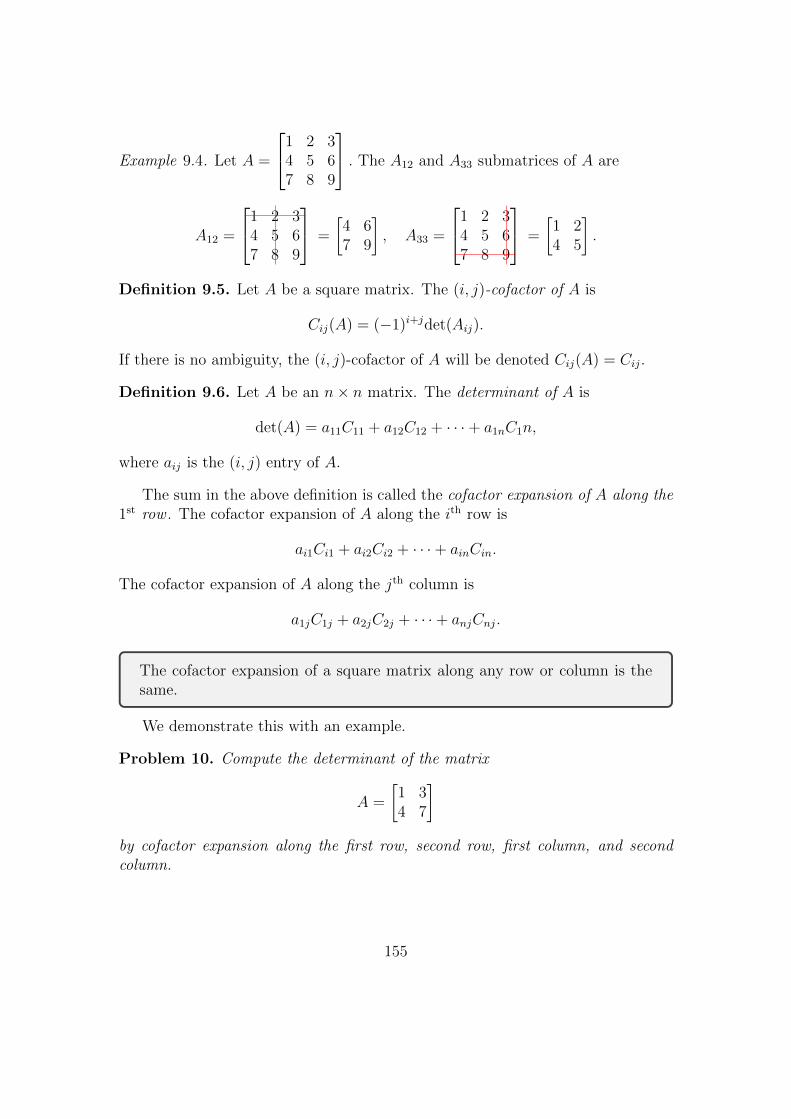
Example 9.4. Let A =
1 2 34 5 67 8 9
. The A12 and A33 submatrices of A are
A12 =
1 2 34 5 67 8 9
=
[4 67 9
], A33 =
1 2 34 5 67 8 9
=
[1 24 5
].
Definition 9.5. Let A be a square matrix. The (i, j)-cofactor of A is
Cij(A) = (−1)i+jdet(Aij).
If there is no ambiguity, the (i, j)-cofactor of A will be denoted Cij(A) = Cij.
Definition 9.6. Let A be an n× n matrix. The determinant of A is
det(A) = a11C11 + a12C12 + · · ·+ a1nC1n,
where aij is the (i, j) entry of A.
The sum in the above definition is called the cofactor expansion of A along the1st row . The cofactor expansion of A along the ith row is
ai1Ci1 + ai2Ci2 + · · ·+ ainCin.
The cofactor expansion of A along the jth column is
a1jC1j + a2jC2j + · · ·+ anjCnj.
The cofactor expansion of a square matrix along any row or column is thesame.
We demonstrate this with an example.
Problem 10. Compute the determinant of the matrix
A =
[1 34 7
]by cofactor expansion along the first row, second row, first column, and secondcolumn.
155

Solution. The submatrices and cofactors of A are computed:
A11 =
[1 34 7
]=[7]
=⇒ c11 = (−1)1+1 det(7) = 7
A12 =
[1 34 7
]=[4]
=⇒ c12 = (−1)1+2 det(4) = −4
A21 =
[1 34 7
]=[3]
=⇒ c21 = (−1)2+1 det(3) = −3
A22 =
[1 34 7
]=[1]
=⇒ c22 = (−1)2+2 det(1) = 1
Therefore, the determinant of A is
det(A) =
a11C11 + a12C12 = 1 · 7 + 3(−4) = −5 (1st row)
a11C11 + a21C21 = 1 · 7 + 4(−3) = −5 (1st column)
a21C21 + a22C22 = 4(−3) + 7 · 1 = −5 (2nd row)
a12C12 + a22C22 = 3(−4) + 7 · 1 = −5 (2nd column). �
The determinant of a 2× 2 matrix[a11 a12a21 a22
]is
det(A) = a11C11 + a12C12
= a11a22 − a12a21.
Check your understanding
Compute det
[1 36 −5
].
Is the matrix invertible?
156

The following statements are equivalent.
• The determinant of a 2× 2 matrix
A =
[a11 a12a21 a22
]equals 0.
• The columns of A, [a11a21
],
[a12a22
]are parallel (the columns are linearly dependent).
• The rows of A are parallel (the rows are linearly dependent).
• The rank of A is less than 2.
• A is not invertible.
Problem 11. Compute det
1 2 34 5 67 8 9
.
Solution. By definition
det
1 2 34 5 67 8 9
= a11C11 + a12C12 + a13C13.
The cofactors are computed:
A11 =
[5 68 9
]=⇒ C11 = (−1)1+1 det
[5 68 9
]= 5 · 9− 8 · 6 = −3
A12 =
[4 67 9
]=⇒ C12 = (−1)1+2 det
[4 67 9
]= −(4 · 9− 7 · 6) = 6
A13 =
[4 57 8
]=⇒ C13 = (−1)1+3 det
[4 57 8
]= 4 · 8− 7 · 5 = −3
157

Therefore, the determinant of A is
det(A) = a11C11 + a12C12 + a13C13
= 1(−3) + 2(6) + 3(−3)
= 0. �
The determinant of a 3× 3 matrix
A =
a11 a12 a13a21 a22 a23a31 a32 a33
is given by the formula
det(A) = a11 det
[a22 a23a32 a33
]− a12 det
[a21 a23a31 a33
]+ a13 det
[a21 a22a31 a32
]= a11(a22a33 − a32a23)− a12(a21a33 − a31a23) + a13(a21a32 − a31a22).
Problem 12. Compute det
−2 −2 −24 3 7−1 0 10
.
Solution. Using the general formula above,
det
−2 −2 −24 3 7−1 0 10
= −2(3 · 10− 7 · 0) + 2(4 · 10− 7(−1))− 2(4 · 0− 3(−1))
= 28. �
In class exercise
Compute the determinant of
A =
1 2 0 45 6 7 80 10 0 013 14 0 16
.Hint: if you choose the right cofactor expansion, the computation will beshorter.
158
In class exercise
Compute the determinant of
A =
1 2 0 40 6 7 80 0 3 00 0 0 8
.Hint: if you choose the right cofactor expansion, the computation will beshorter.
The determinant of an upper (or lower) trianglular matrix equals the productof the diagonal entries.
9.2 Properties of the determinant
In the previous section, we observed the following fact in some examples.
Theorem 9.7. Let A be a square matrix. The determinant of A is equal to thecofactor expansion of A along any row or column.
From this theorem, we can deduce some properties of determinants.
Properties of the determinant:
Let A be a square matrix.
(a) If A has a row or column of zeros, then its determinant equals zero.
(b) det(A) = det(AT ).
Proof. (a) Cofactor expanding along the zero row or zero column proves thatthe determinant is zero.
(b) Since the rows of A are equal to the columns of AT , cofactor expanding Aalong rows gives the same result as cofactor expanding AT along columns.
159

Suppose that A is a square matrix with two identical rows. Then the deter-minant of A is zero.
In class exercise
Compute the determinants of the following matrices.
A =
2 0 00 5 00 0 −1
, B =
0 0 −10 5 02 0 0
,
C =
2 0 00 10 00 0 −1
, D =
2 0 −10 5 00 0 −1
.What elementary row operations were performed to obtain B,C, and D fromthe matrix A?
The following theorem, in particular, relates determinants to elementary rowoperations.
Theorem 9.8. Let A be a square matrix. Elementary row operations performedon the matrix A change the determinant of A in the following ways:
(a) Interchanging two rows of A changes the sign of the determinant. That is,
if ARi↔Rj−→ A′, then
det(A′) = − det(A).
(b) Multiplying a row by a scalar c multiplies the determinant by c. That is, if
ARj→cRj−→ A′, then
det(A′) = c det(A).
(c) Adding a multiple of one row to another leaves the determinant unchanged.
That is, if ARi→Ri+cRj−→ A′, then
det(A′) = det(A).
We saw earlier in the course that a 2× 2 matrix is invertible if and only if thedeterminant is not zero. In fact, this is true in general.
Theorem 9.9. Let A be a n×n matrix. The following statements are equivalent.
160

(a) A is invertible.
(b) det(A) 6= 0.
The next most important property of the determinant is the following multi-plicative property.
Theorem 9.10 (Multiplicative property of the determinant). Let A and B ben× n matrices. Then,
det(AB) = det(A) det(B).
This theorem is actually tricky to prove. The left hand side of the equation inthe above theorem involves matrix multiplication while the right hand side involvesregular multiplication.
More properties of the determinant:
Let A, A1, . . . , Ak be n× n matrices.
(a) det(A1A2 · · ·Ak) = det(A1) det(A2) · · · det(Ak).
(b) If k is a positive integer, then det(Ak) = det(A)k.
(c) If A is invertible, then det(A−1) = det(A)−1.
(d) If c ∈ R, then det(cA) = cn det(A).
(e) det(AB) = det(BA), even when AB 6= BA.
Warning
In general, there is no nice formula relating det(A+B) and det(A)+det(B).
We finish this section by adding one more item to our long list of equivalentstatements for square matrices.
Theorem 9.11 (The big theorem for n×n matrices, part 3). Suppose A is a n×nmatrix. The following statements are equivalent:
(a) The matrix A is invertible.
(b) The matrix equation Ax = b has exactly one solution for all n × 1 columnvectors b.
161

(c) The homogeneous matrix equation Ax = 0 has exactly one solution (thetrivial solution).
(d) The rank of A is n.
(e) The reduced row-echelon form of A is I.
(f) There exists a n× n matrix B such that AB = I.
(g) There exists a n× n matrix B such that BA = I.
(h) A can be written as a product of elementary matrices.
(i) The linear transformation TA : Rn → Rn is invertible.
(j) The linear transformation TA : Rn → Rn is injective (ker(TA) = {0}).
(k) The linear transformation TA : Rn → Rn is surjective (im(TA) = Rn).
(l) null(A) = {0}.
(m) col(A) = Rn.
(n) row(A) = Rn.
(o) det(A) 6= 0.
9.3 Determinants and area
There is a simple relationship between determinants and areas.
Theorem 9.12. Let D be a region of finite area in R2. Let TA : R2 → R2 be thelinear transformation TA(x) = Ax. Then,
area(T (D)) = | det(A)|area(D).
This is illustrated in the following examples.
Example 9.13 (Scaling in the y-direction). Let T : R2 → R2 be given by
T
([xy
])=
[x3y
].
The linear transformation T maps the unit square as follows:
162

x
y
Area = 1
x
y
Area = 3
T
T ( 10 ) = ( 1
0 )T ( 0
1 ) = ( 03 )
The map T sends the unit square (with area one) to the rectangle (with areathree). The map T scales area by three. It is straightforward to check that thedeterminant of the matrix representing T is three.
Example 9.14 (Shear in the x-direction). Let T : R2 → R2 be given by
T
[xy
]=
[1 20 1
] [xy
]=
[x+ 2yy
].
The map T acts on the unit square as in the picture:
x
y
Area = 1
x
y
Area = 1
T
T ( 10 ) = ( 1
0 )T ( 0
1 ) = ( 21 )
The linear transformation T does not change the area, and it is easy to check thatthe determinant of the matrix representing T is one. (The fact that a shear doesnot change the areas is an example of “Cavalieri’s principle.”)
Problem 13. What is the area of enclosed by the ellipse
x2
a2+y2
b2= 1?
9.4 Application: multivariable integration and
the determinant of the Jacobian
163

Key concepts from Chapter 9
Definition of the determinant using cofactor expansions, computing determi-nants using cofactor expansions, properties of determinants, determinants ofelementary matrices, determinants of products of matrices, det(A) 6= 0 iff Ais invertible, determinants of 2× 2 matrices and area.
164

Chapter 10
Eigenvalues and eigenvectors
10.1 Eigenvalues and Eigenvectors
Definition 10.1. Let A be an n × n matrix. If there is a scalar λ ∈ R and anon-zero vector u ∈ Rn such that
Au = λu,
then λ is an eigenvalue of A and u is an eigenvector of A corresponding to theeigenvalue λ.
Example 10.2. For each of the following 2 × 2 matrices, find all the eigenvaluesand corresponding eigenvectors by using the definition.
(a) A =
[2 00 −5
].
(b) A = 110
[1 33 9
].
(c) A =
[1 10 1
].
(d) A =
[0 10 0
].
(e) A =
[0 11 0
].
(f) A =
[0 00 0
].
165

(g) A =
[0 −11 0
].
(h) A =
[1 22 1
].
Give a geometric description of the linear transformation TA : R2 → R2 corre-sponding to each matrix A.
10.2 Computing eigenvalues and eigenvectors
To compute the eigenvalues and eigenvectors of a matrix A, it is easiest to firstfind the eigenvalues of A and then find the corresponding eigenvectors.
The following statements are equivalent:
(a) Au = λu for some non-zero vector u.
(b) (A− λI)u = 0 for some non-zero vector u.
(c) null(A− λI) 6= {0}.
(d) A− λI is not invertible.
(e) det(A− λI) = 0.
The last item on this list of equivalent statments provides a method for com-puting eigenvalues of a matrix.
Definition 10.3. The polynomial
cA(λ) = det(A− λI)
is called the characteristic polynomial of A.
The eigenvalues of A are the roots of the polynomial
cA(λ) := det(A− λI).
166

Computing Eigenvalues of a square matrix
Given a n×n matrix A, its eigenvalues can be computed in the following way.
1. Compute the characteristic polynomial cA(λ) = det(A− λI) by computingthe determinant of A− λI.
2. Compute the roots of cA(λ) (i.e. values of λ that solve the equation cA(λ) =0). The roots are the eigenvalues of A.
Problem 14. Compute the eigenvalues of the matrix
A =
[2 11 2
].
Solution. The eigenvalues of A are the roots of its characteristic polynomial cA(x).
cA(λ) = det
([2 11 2
]− λ
[1 00 1
])= det
[2− λ 1
1 2− λ
]= (2− λ)2 − 1
= λ2 − 4λ+ 3
= (λ− 3)(λ− 1).
Since the roots of cA(λ) are 3 and 1, the eigenvalues of A are 3 and 1.
In-class exercise
Use the characteristic polynomial to compute the eigenvalues of the followingmatrices.
A =
[0 11 0
], B =
[2 10 2
], C =
[1 10 2
].
The last result in this subsection relates the eigenvalues of a square matrix toits invertibility.
Let A be a square matrix. The following statements are equivalent:
(a) The matrix A is invertible.
(b) 0 is not an eigenvalue of A
167

Check your understanding
Suppose that A is a square matrix and det(A) = 3. Is 0 an eigenvalue of A?
10.3 Eigenspaces
The following statements are equivalent:
(a) u is an eigenvector of A corresponding to the eigenvalue λ.
(b) u is a nonzero vector and u ∈ null(A− λI).
Definition 10.4. Let A be a square matrix and let λ be an eigenvalue of A. Theeigenspace of A corresponding to the eigenvalue λ is the set
Eλ(A) := null(A− λI).
Since it is defined as the null space of a matrix,
Eigenspaces, Eλ(A), of an n× n matrix A are subspaces of Rn.
Problem 15. Find a basis for R2 consisting of eigenvectors of
A =
[2 11 2
].
Solution. From problem 14, the eigenvalues of A were found to be
λ1 = 3 and λ2 = 1.
In order to find a basis for R2 consisting an eigenvectors of A, a basis will be foundfor each eigenspace of A, and taken together, these will form a basis for A.
The eigenspaces of A are computed as follows:
E3(A) = null
([2 11 2
]− 3
[1 00 1
])= null
[−1 11 −1
]= span
{[11
]}.
168

Therefore, a basis for E3(A) is {[11
]}.
Similarly,
E1(A) = null
([2 11 2
]−[1 00 1
])= null
[1 11 1
]= span
{[−11
]}.
Therefore, a basis for E1(A) is {[−11
]}.
So, a basis for R2 consisting of eigenvectors of A is{[11
],
[−11
]}.
�
Problem 16. Find the eigenvalues of the matrix
A =
1 2 −11 0 14 −4 5
.Write each eigenspace of A as spanning set.
Solution. The eigenvalues of A are the roots of its characteristic polynomial:
cA(λ) = det
1 2 −11 0 14 −4 5
− λ1 0 0
0 1 00 0 1
= det
1− λ 2 −11 −λ 14 −4 5− λ
= −λ3 + 6λ2 − 11λ+ 6.
169

After applying the rational roots theorem and using polynomial long division (orusing a calculator), the characteristic polynomial factors as
cA(λ) = −λ3 + 6λ2 − 11λ+ 6
= −(λ− 3)(λ− 2)(λ− 1).
The eigenvalues of A are the roots of its characteristic polynomial: 3, 2, and 1.The eigenspaces of A are
E3(A) = null(A− 3I) = null
−2 2 −11 −3 14 −4 2
= span
−1
14
E2(A) = null(A− 2I) = null
−1 2 −11 −2 14 −4 3
= span
−2
14
E1(A) = null(A− I) = null
0 2 −11 −1 14 −4 4
= span
−1
12
. �
In-class exercise
Compute the eigenspaces corresponding to each eigenvalue of the followingmatrices.
A =
[0 11 0
], B =
[1 00 1
], C =
[1 10 1
].
10.4 Algebraic multiplicity of eigenvalues
Example 10.5. Let p(λ) = (λ− 3)4(λ− 1)(λ− 4)2. The root 3 has multiplicity 4.The root 1 has multiplicity 1. The root 4 has multiplicity 2.
Definition 10.6. Suppose λ is an eigenvalue of A. The algebraic multiplicity ofthe eigenvalue λ is the multiplicity of λ as a root of the characteristic polynomial,cA.
170

Check your understanding
Let A =
2 0 0 00 2 0 00 0 3 00 0 0 1
.
What are the eigenvalues of A? What are their algebraic multiplicities?
The next theorem relates the multiplicity of an eigenvalue of a matrix to thedimension of the corresponding eigenspace.
Theorem 10.7. Let A be a square matrix. Suppose that λ is an eigenvalue of Awith algebraic multiplicity m. Then,
1 ≤ dim(Eλ(A)) ≤ m.
In-class exercise
For each matrix below, compare the algebraic multiplicity of the eigenvalue1, and the dimension of the eigenspace E1.
A =
[0 11 0
], B =
[1 00 1
], C =
[1 10 1
].
10.5 Diagonalization
Diagonal matrices are great for a bunch of reasons:
• They commute. If A and B are both diagonal, then AB = BA.
• We can easily see what their eigenvalues and eigenvectors are.
• The linear transformation TA of a diagonal matrix A acts on Rn in a verysimple way.
• It is easy to compute their determinants and check if they are invertible.
• If a diagonal matrix is invertible, it is easy to compute its inverse.
• Computing products of diagonal matrices takes less time (computationally)than computing a product of two matrices in general.
171

Definition 10.8. A square matrix A is diagonalizable if there exists a diagonalmatrix D and an invertible matrix P such that
A = PDP−1.
A square matrix A is diagonalizable if and only if it has n linearly indepen-dent eigenvectors.
Check your understanding
Which of the matrices below are diagonalizable?
A =
[0 11 0
], C =
[1 10 1
], D =
[0 −11 0
].
Diagonalizing a matrix:
In order to diagonalize a n× n matrix A,
1. Compute the eigenvalues of A. (if the characteristic polynomial does notfactor completely, then A is not diagonalizable).
2. Compute the eigenspaces of each of the eigenvalues of A.
At this point, there are two possibilities.
(a) If the dimensions of the eigenspaces of A add to n (for each eigenvalueλ, dim(Eλ) = mλ), then A is diagonalizable. The matrices P and D canthen be computed from a basis for the eigenspaces of A (see examplesbelow).
(b) Otherwise (if the dimensions of the eigenspaces don’t add to n), then Ais not diagonalizable.
Problem 17. Let
A =
1 2 −11 0 14 −4 5
.Diagonalize A. That is, find a diagonal matrix D and an invertible matrix P suchthat A = PDP−1.
172

Solution. It can be verified (as an exercise!) that
• The eigenvalues of A are 1, 2, and 3.
• The corresponding eigenspaces are
E1(A) = span
−1
12
, E2(A) = span
−2
14
, and,
E3(A) = span
−1
14
.
• A basis for R3 consisting of eigenvectors of A is
β =
−1
12
,−2
14
,−1
14
.
Using the observations from the previous example, choose the change of basis ma-trix P to be
P =
−1 −2 −11 1 12 4 4
=⇒ P−1 =
0 2 −12
−1 −1 01 0 1
2
and choose the diagonal matrix
D =
1 0 00 2 00 0 3
.Note that the diagonal entries of D are the eigenvalues of A and the columns of Pare eigenvectors of A, which are in a corresponding order to the eigenvalues alongthe diagonal of D.
It can be checked (as an exercise!) that
A = PDP−1,
which solves the problem. �
173

It is particularly important to note that the diagonalizability of an n×n matrixdepends on whether or not that matrix has n linearly independent eigenvectors.Therefore, it is important to know when a matrix has linearly independent eigen-vectors. The following theorems provide helpful information on determining thelinear independence of the eigenvectors of a matrix.
Theorem 10.9. Let A be a square matrix. If u1, . . . , uk are eigenvectors of Acorresponding to k distinct eigenvalues, then the set {u1, . . . , uk} is linearly inde-pendent.
This theorem will be proven at the end of this subsection. Its proof will be viainduction, and can be skipped.
Let A be an n× n matrix. If A has n distinct eigenvalues, then A is diago-nalizable.
Recall that if A is a square matrix and and λ is an eigenvalue of A withmultiplicity m, then,
1 ≤ dimEλ(A) ≤ m.
Suppose that A is a square matrix and the characteristic polynomial of Afactors fully (that is, it factors entirely into linear terms, with no irreduciblequadratic terms). Then, if A has eigenvalues λ1, . . . , λk with multiplicitiesm1, . . . ,mk, the following statements are equivalent:
(a) the matrix A is diagonalizable
(b) for each 1 ≤ i ≤ k,
dimEλi(A) = mi for all i.
Problem 18. Is H =
4 −1 −2−6 3 48 −2 −4
diagonalizable?
Solution. The characteristic polynomial of H is
cH(x) = det
4 −1 −2−6 3 48 −2 −4
= (4− x)[(3− x)(−4− x) + 8] + [−6(−4− x)− 32]− 2[12− 8(3− x)]
= −x(x− 1)(x− 2).
174
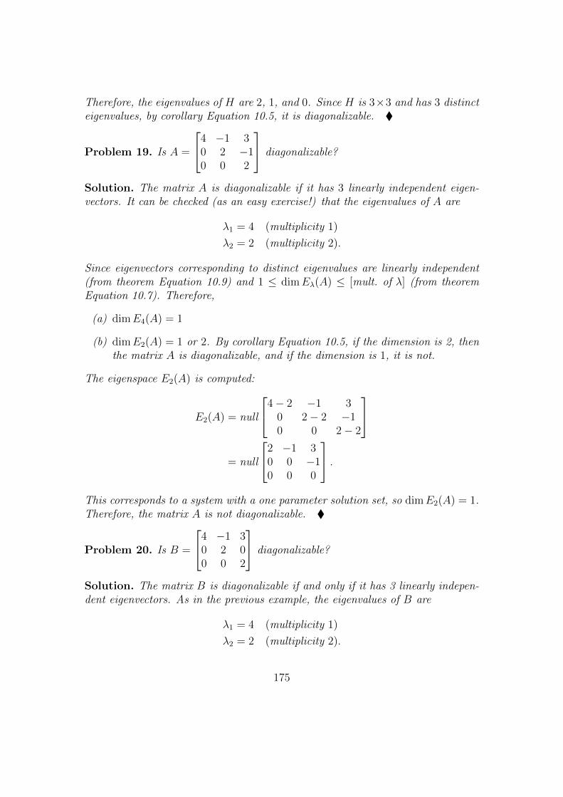
Therefore, the eigenvalues of H are 2, 1, and 0. Since H is 3×3 and has 3 distincteigenvalues, by corollary Equation 10.5, it is diagonalizable. �
Problem 19. Is A =
4 −1 30 2 −10 0 2
diagonalizable?
Solution. The matrix A is diagonalizable if it has 3 linearly independent eigen-vectors. It can be checked (as an easy exercise!) that the eigenvalues of A are
λ1 = 4 (multiplicity 1)
λ2 = 2 (multiplicity 2).
Since eigenvectors corresponding to distinct eigenvalues are linearly independent(from theorem Equation 10.9) and 1 ≤ dimEλ(A) ≤ [mult. of λ] (from theoremEquation 10.7). Therefore,
(a) dimE4(A) = 1
(b) dimE2(A) = 1 or 2. By corollary Equation 10.5, if the dimension is 2, thenthe matrix A is diagonalizable, and if the dimension is 1, it is not.
The eigenspace E2(A) is computed:
E2(A) = null
4− 2 −1 30 2− 2 −10 0 2− 2
= null
2 −1 30 0 −10 0 0
.This corresponds to a system with a one parameter solution set, so dimE2(A) = 1.Therefore, the matrix A is not diagonalizable. �
Problem 20. Is B =
4 −1 30 2 00 0 2
diagonalizable?
Solution. The matrix B is diagonalizable if and only if it has 3 linearly indepen-dent eigenvectors. As in the previous example, the eigenvalues of B are
λ1 = 4 (multiplicity 1)
λ2 = 2 (multiplicity 2).
175

And, as in the previous problem, the dimension of E2(A) needs to be determined.If the dimension is 2, then A is diagonalizable. If the dimension is 1, then A isnot diagonalizable. The dimension is computed:
E2(A) = null
2 −1 30 0 00 0 0
.This is a 2 dimensional subspace. Therefore, A is diagonalizable. �
Now, theorem Equation 10.9 is proven:
Proof of theorem Equation 10.9. It needs to be shown that if u1, . . . , uk are eigen-vectors of a matrix A corresponding to distinct eigenvalues, then those vectorsform a linearly independent set. The proof proceeds by induction.
Base case: Suppose that there is only one eigenvector, u1. Then, since eigen-vectors are non-zero by definition, the set {u1} is linearly independent.
Induction hypothesis: Suppose that the theorem is true for when there are k eigen-vectors.
Inductive step: Suppose that u1, . . . , uk, uk+1 are k+ 1 eigenvectors for the matrixA corresponding to k+1 distinct eigenvalues λ1, . . . , λk+1. Then, these vectors arelinearly independent if the only solution to
a1u1 + · · ·+ akuk + ak+1uk+1 = 0 (10.10)
is a1 = · · · = ak+1 = 0.The linear map T given by T (x) = Ax is applied to equation (10.10). Since
T (0) = 0, this equation becomes
0 = A(a1u1 + · · ·+ akuk + ak+1uk+1)
= λ1a1u1 + · · ·+ λkakuk + λk+1ak+1uk+1. (10.11)
Then, subtracting λk+1(a1u1 + · · ·+ akuk + ak+1uk+1) from both sides of equation(10.11), and noting that a1u1 + · · ·+ akuk + ak+1uk+1 = 0 by assumption, yields
0 = a1(λ1 − λk+1)u1 + · · ·+ ak(λk − λk+1)uk + ak+1(λk+1 − λk+1)uk+1
= a1(λ1 − λk+1)u1 + · · ·+ ak(λk − λk+1)uk. (10.12)
Then, by the induction hypothesis, all of the coefficients in equation (10.12) mustbe zero. Since all of the eigenvalues are distinct, this implies that a1 = · · · = ak =0. Hence, equation (10.10) reduces to
0 = ak+1uk+1,
176

which is only possible if ak+1 = 0. Therefore, all of the coefficients a1, . . . , ak+1
are zero, and the set of eigenvectors is linearly independent, which concludes theproof.
10.6 Application: google page rank
10.7 Application: eigenvalues and eigenvectors
in classical and quantum mechanics
177

Key concepts from Chapter 10
Definition of eigenvalues and eigenvectors, the characteristic polynomial,computing eigenvalues, computing eigenspaces, properties of eigenvalues andeigenspaces, diagonalizing a matrix.
178

Chapter 11
Orthogonality
Orthogonal projection in R2. Pictures.
11.1 Orthogonality
Recall that two nonzero vectors u and v are called “orthogonal” if u ·v = 0. If thetwo vectors are non-zero, then this means that the angle formed by two orthogonalvectors is π/2.
Warning
The vector 0 is orthogonal to every vector, since 0 · u = 0.
Definition 11.1. A set {u1, . . . ,uk} of k vectors in Rn is called an orthogonal setif whenever i 6= j, the vectors ui and uj are orthogonal.
Definition 11.2. A set {u1, . . . ,uk} of k non-zero vectors in Rn is an orthonormalset if it is an orthogonal set with the additional property that every vector in theset is a unit vector.
In-class exercise
Is
1
11
,−3
12
,−1
5−4
an orthogonal set?
Is
1
21
, 0
1−2
,−2
10
an orthogonal set?
179
Theorem 11.3. An orthogonal set of nonzero vectors is linearly independent.
Proof. Let {u1, . . . ,uk} be an orthogonal set of nonzero vectors. It needs to beshown that the only solution to the equation
0 = x1u1 + · · ·+ xkuk
is the trivial solution x1 = · · · = xk = 0.
For each i, we can take the dot product of this equation with ui,
0 = x1u1 + · · ·+ xkuk
⇒ 0 · ui = (x1u1 + · · ·+ xkuk) · ui⇒ 0 = x1(u1 · ui) + · · ·+ xi(ui · ui) + · · ·+ xk(uk · ui)⇒ 0 = x1(0) + · · ·+ xi(ui · ui) + · · ·+ xk(0) since ui · uj = 0
⇒ 0 = xi(ui · ui)⇒ 0 = xi since ui 6= 0
Thus, for every i, xi = 0, so we have shown that the only solution to the equation
0 = x1u1 + · · ·+ xkuk
is the trivial solution; in other words, the set {u1, . . . ,uk} is linearly independent.
Recall that a set is a basis for a subspace if it spans the subspace and is linearlyindependent. Thus, the theorem above tells us that any orthogonal set which spansa subspace is automatically a basis for that subspace.
Definition 11.4. An orthogonal set that is also a basis for a subspace S is calledan orthogonal basis of S. An orthonormal set that is also a basis for a subspaceS is called an orthonormal basis of S.
Example 11.5. The set of standard unit vectors {e1, . . . , en} is an orthonormalbasis for Rn since
• The set {e1, . . . , en} is orthogonal, since ei · ej = 0 whenever i 6= j.
• The set {e1, . . . , en} is a basis for Rn (we checked this in Chapter 7).
• The vectors are unit vectors: ||ei|| = 1 for every 1 ≤ i ≤ n.
Example 11.6. As we saw in the previous example, the standard basis for Rn is anorthonormal basis. Of course, there are many other orthogonal and orthonormalbases. In this example we describe different orthogonal bases of R2 and R3.
180

(a) As we saw above, the standard basis
{[10
],
[01
]}is an orthonormal basis
for R2.
(b) If we rotate the two vectors in the standard basis for R2 by some angle θ,then the result is a different orthonormal basis. Using the rotation matrix,[
cos(θ) − sin(θ)sin(θ) cos(θ)
] [10
]=
[cos(θ)sin(θ)
][cos(θ) − sin(θ)sin(θ) cos(θ)
] [01
]=
[− sin(θ)cos(θ)
]The new set of vectors is thus{[
cos(θ)sin(θ)
],
[− sin(θ)cos(θ)
]}.
This set is orthogonal since[cos(θ)sin(θ)
]·[− sin(θ)cos(θ)
]= − sin(θ) cos(θ) + sin(θ) cos(θ) = 0.
Thus this new set gives an orthogonal basis for R2. Furthermore, for each ofthe two vectors in this set, we see that∣∣∣∣∣∣∣∣ [cos(θ)
sin(θ)
] ∣∣∣∣∣∣∣∣ =√
cos2(θ) + sin2(θ) = 1∣∣∣∣∣∣∣∣ [− sin(θ)cos(θ)
] ∣∣∣∣∣∣∣∣ =√
(− sin(θ))2 + cos2(θ) = 1
(c) If we scale the two vectors in the standard basis for R2 by non-zero num-
bers then we still have an orthogonal basis. For instance
{[30
],
[02
]}is an
orthogonal basis for R2, but it is not an orthonormal basis.
(d) The basis
1
00
,0
10
is an orthonormal basis for the subspace S ⊆ R2
defined as
S =
xy
0
∈ R3 : x, y ∈ R
181

which is a plane in R3 (sometimes called the xy-plane in R3).
The linear transformation of R3 “rotation by an angle of θ in the xy-plane”is described by the matrix cos(θ) − sin(θ) 0
sin(θ) cos(θ) 00 0 1
If we apply this transformation to the vectors in the basis for S above, weget a different orthonormal basis for S,
cos(θ)sin(θ)
0
,− sin(θ)
cos(θ)0
There is a straightforward formula for writing a vector u as a linear combina-
tion of the vectors s1, . . . , sk in an orthogonal basis.
Let β = {s1, . . . , sk} be an orthogonal basis for a subspace S. If u ∈ S, then
u =
(u · s1‖s1‖2
)s1 +
(u · s2‖s2‖2
)s2 + · · ·+
(u · sn‖sn‖2
)sn
= projs1u + projs2u + · · ·+ projsnu.
Proof. Since β is a basis, we know the vector x can be written uniquely as
u = c1s1 + c2s2 + · · ·+ cnsn
for some coefficients c1, . . . , cn ∈ R. By taking the dot product of u with the basisvector si, the coefficient ci can be computed, as follows.
u · si = (c1s1 + c2s2 + · · ·+ cnsn) · si= c1(s1 · si) + · · ·+ ci(si · si) + · · ·+ cn(sn · si)= ci(si · si) (since sj · si = 0 for all i 6= j)
= ci ‖si‖2 .
Rearranging yields
ci =u · si‖si‖2
.
182

In-class exercise
Show that the sets1 =
1−130
, s2 =
−2111
, s3 =
1101
, s4 =
1103−11
.
is orthogonal by computing dot-products of every pair of vectors in the set.
Normalize the vectors in this basis to turn it into an orthonormal basis forR4.
Since the set β in the previous exercise is orthogonal, we know that
• Since β is orthogonal, it is linearly independent.
• Since β is a set of 4 linearly independent vectors in R4, it is a basis for R4.
• Thus we can conclude that β is an orthogonal basis for R4.
Problem 21. Write the vector (1, 3, 2, 4) as a linear combination of the vectorsin the orthogonal basis β from the previous exercise.
Solution. The formula above is applied:1324
=4
11
1−130
+7
7
−2111
+8
3
1101
+−7
231
1103−11
. �
11.2 Orthogonal complements
Definition 11.7. Let S be a subspace of Rn. The orthogonal complement of S isthe set
S⊥ = {x ∈ Rn : x · s = 0 for all s ∈ S}.
Example 11.8. The orthogonal complement of a subspace of R2 or R3 is easy tovisualize and understand geometrically.
(a) In R2:
183

• The orthogonal complement of the trivial subspace {0} is the set
{0}⊥ = {x ∈ R2 : x · 0 = 0} = R2.
• The orthogonal complement of a line through the origin spanned by anon-zero vector u, L = span{u} = {tu : t ∈ R}, is the set
L⊥ = {x ∈ R2 : x · (tu) = 0 for all t ∈ R} = {x ∈ R2 : x · u = 0}.
This set is simply the line through the origin orthogonal to u.
• The orthogonal complement of the subspace R2 is the set
(R2)⊥ = {x ∈ R2 : x · y = 0 for all y ∈ R2} = {0}.
(b) In R3:
• Similar to the case in R2, the orthogonal complement of the trivialsubspace {0} is the set
{0}⊥ = {x ∈ R3 : x · 0 = 0} = R3.
• The orthogonal complement of a line through the origin in R3 spannedby a non-zero vector u, L = span{u} = {tu : t ∈ R}, is the set
L⊥ = {x ∈ R3 : x · (tu) = 0 for all t ∈ R} = {x ∈ R3 : x · u = 0}.
This set is simply the plane through the origin orthogonal to u. This isthe plane through the origin in R3 determined by the normal vector u.
• Suppose that P = span{u,v} is a plane through the origin in R3 (inparticular the two vectors are linearly independent). The orthogonalcomplement of P is
P⊥ ={x ∈ R3 : x · (su + tv) = 0 for all s, t ∈ R
}={x ∈ R3 : x · u = 0 and x · v = 0
}There are several ways to express this set. One particularly instructivething is to observe that{
x ∈ R3 : x · u = 0 and x · v = 0}
= null
([u1 u2 u3v1 v2 v3
]).
We also know from the tutorials that when u and v are not parallel
null
([u1 u2 u3v1 v2 v3
])= span{u× v}.
In other words, the subspace P⊥ equals the line through the originorthogonal to P .
184

• Finally, (R3)⊥ = {0}.
The following fact is useful for computing the orthogonal complement of a sub-space.
Theorem 11.9. Let A be a m× n matrix. Then
row(A)⊥ = null(A).
Proof. To show these two subspaces are equal, we show both inclusions: row(A)⊥ ⊆null(A) and null(A) ⊆ row(A)⊥.
The key step in this proof is to remember that, by definition of matrix multi-plication, if A is a matrix with rows u1, . . . ,um, then
Ax =
u1 · x...
um · x
.• First, we show that row(A)⊥ ⊆ null(A).
If x ∈ row(A)⊥, then u1 · x = 0 for all 1 ≤ i ≤ m, so
Ax =
u1 · x...
um · x
=
0...0
,so x ∈ null(A).
• Second, we show that null(A) ⊆ row(A)⊥.
If x ∈ null(A), then we know that Ax = 0. Thus we know thatu1 · x...
um · x
=
0...0
.This tells us that x is orthogonal to the vectors u1, . . . ,um.
185

Since row(A) = span{u1, . . . ,um}, we know that for any y = t1u1 + · · · +tmum ∈ row(A),
x · y = x · (t1u1 + · · ·+ tmum)
= t1x · u1 + · · ·+ tmx · um= 0
Thus x ∈ row(A)⊥.
Any subspace S ⊆ Rn can be expressed as the row space of a matrix (just takethe vectors in a spanning set and write them as the rows of a matrix). Since thenull space of a matrix is a subspace of Rn, Theorem 11.9 immediately tells us that
If S is a subspace of Rn, then the orthogonal complement, S⊥, is also asubspace of Rn.
By the rank-nullity theorem, we know that for a m× n matrix A,
dim(row(A)) + dim(null(A)) = n.
Combining this with Theorem 11.9, we see that
dim(row(A)) + dim(row(A)⊥) = dim(row(A)) + dim(null(A)) = n.
This gives us the following result.
If S is a subspace of Rn, then
dim(S) + dim(S⊥) = n.
Theorem 11.9 also gives us an algorithm for computing a basis for the orthog-onal complement of a subspace.
Algorithm for computing the orthogonal complement of a sub-space:
If we are given a subspace S ⊆ Rn as the span of a set of vectors S =span{u1, . . . ,um}, then we can compute a basis for S⊥ as follows:
186

1. Make the vectors u1, . . . ,um the rows of a m× n matrix A.
2. Compute a basis for null(A) = S⊥ by computing the basic solutions.
Problem 22. Let
S = span
b1 =
1−2−210
, b2 =
−243−12
.
Find a basis for S⊥.
Solution. By Theorem 11.9,
S⊥ = null
[1 −2 −2 1 0−2 4 3 −1 2
].
Computing basic solutions of this matrix, we see that
21000
,
10110
,
40201
is a basis for this null space, which makes it a basis for S⊥. �
We end this section by observing that since for any matrix A,
row(AT ) = col(A),
Theorem 11.9 immediately implies the following fact.
If A is a m× n matrix, then
col(A)⊥ = null(AT ).
(note that these are both subspaces of Rm)
Proof. Applying Theorem 11.9 to the matrix AT we have that
col(A)⊥ = row(AT )⊥ = null(AT ).
187
11.3 Orthogonal projection onto a subspace
Recall that a nonzero vector u ∈ Rn spans a line L = span{u}. In Chapter 5 westudied the following problem:
The problem of orthogonal projection onto a line:
Given a vector v ∈ Rn, find vectors v1 and v2 so that
• v = v1 + v2
• v1 is parallel to u (contained in the line L) and v2 is orthogonal to u(contained in the hyperplane normal to u).
In Chapter 5, we discovered that we can always find such vectors, and they aregiven by formulas:
v1 = projuv =v · uu · u
u
v2 = v − projuv = v − v · uu · u
u.
Given a subspace S of Rn, we would like to solve a similar problem.
The problem of orthogonal projection onto a subspace:
Given a vector v ∈ Rn, find vectors v1 and v2 so that
• v = v1 + v2
• v1 is contained in S and v2 is orthogonal to S (contained in S⊥).
The solution to this problem is similar to the solution to the problem of or-thogonal projection onto a line.
• First, suppose that {u1, . . . ,uk} is an orthogonal basis for S. Since it is abasis, we know that v1 ∈ S can be written as
v1 = x1u1 + · · ·+ xkuk
for some coefficients x1, . . . , xk.
188
• We can solve for the coefficients x1, . . . , xk one by one. For each ui, we seethat
ui · v = ui · (v1 + v2)
= ui · v1 + ui · v2
= ui · (x1u1 + · · ·+ xkuk)
= x1(ui · u1) + · · ·+ xk(ui · uk)= xi(ui · ui)
Thus we see thatxi =
ui · vui · ui
sov1 =
u1 · vu1 · u1
u1 + · · ·+ uk · vuk · uk
uk = proju1v + · · ·+ projuk
v
Definition 11.10. Let S be a non-zero subspace. Let {u1, . . . ,uk} be an orthog-onal basis for S. The orthogonal projection of v onto S is denoted projSv andgiven by the formula
projSv =u1 · vu1 · u1
u1 + · · ·+ uk · vuk · uk
uk = proju1v + · · ·+ projuk
v.
Example 11.11. Consider the subspace S = {(x, y, 0) ∈ R3 : x, y ∈ R}. Theorthogonal projection of v = [8 6 − 9] onto S can be computed using the basis{e1, e2} for S:
projSv = proje1v + proje2v =
860
∈ S• The vector v2 is then found by rearranging the equation
v = v1 + v2
to solve for v2,
v2 = v − v1 = v − proju1v − · · · − projuk
v
• The vector v2 is orthogonal to S, since for every ui in the orthogonal basisfor S above,
ui · v2 = ui · (v − proju1v − · · · − projuk
v)
= ui · v − ui · proju1v − · · · − ui · projuk
v
= ui · v − ui · projuiv
= ui · v − ui ·(
ui · viui · ui
ui
)= 0
Thus v2 ∈ S⊥.
189

We call the vector v2 the projection of v orthogonal to S. It is sometimes denotedprojS⊥v.
Example 11.12. Continuing from the previous example, the subspace S⊥ = {(0, 0, z) ∈R3 : z ∈ R}. The projection of v = [8 6 − 9] orthogonal to S is
projS⊥v = v − projSv =
00−9
∈ SSimilar to orthogonal projection onto lines, orthogonal projection onto sub-
spaces has several properties:
Properties of orthogonal projection:
Suppose S is a subspace of Rn. Then
• T (x) = projS(x) is a linear transformation with
– ker(T ) = S⊥
– im(T ) = S.
• For any vector v ∈ Rn, projS(v) ∈ S.
• If v ∈ S, then projS(v) = v.
• If v ∈ S⊥, then projS(v) = 0.
Problem 23. The set 2−21
, 2
1−2
is orthogonal. Compute the projection of
774
onto S = span
2−21
, 2
1−2
.
Solution. Apply the definition of projection onto a subspace (Equation 11.10):
projs
774
=4
9
2−21
+13
9
21−2
. �
190

11.4 The Gram-Schmidt algorithm
In this section, we describe an algorithm for solving the following problem.
Given a basis {u1, . . . ,uk} for a subspace S ⊆ Rn, find an orthogonal basisfor S.
Let’s try to do this for a simple example.
Problem 24. Find an orthogonal basis for the subspace S = span
2
10
,1
01
.
The Gram-schmidt algorithm
Suppose that {u1, . . . ,uk} is a basis for a subspace S ⊆ Rn. In order tocompute an orthogonal basis for S, compute
v1 = u1
v2 = u2 − projv1u2
v3 = u3 − projv1u3 − projv2
u3
...
vk = uk − projv1uk − projv2
uk − · · · − projvk−1uk.
By construction, the set {v1, . . . ,vk}, is an orthogonal basis for S.
Further, the set {v1
‖v1‖, . . . ,
vk‖vk‖
}.
is an orthonormal basis for S.
Problem 25. The set
1110
,−10−11
,−100−1
is a basis for its span, which is a subspace of R4. Transform this basis into anorthogonal basis.
191
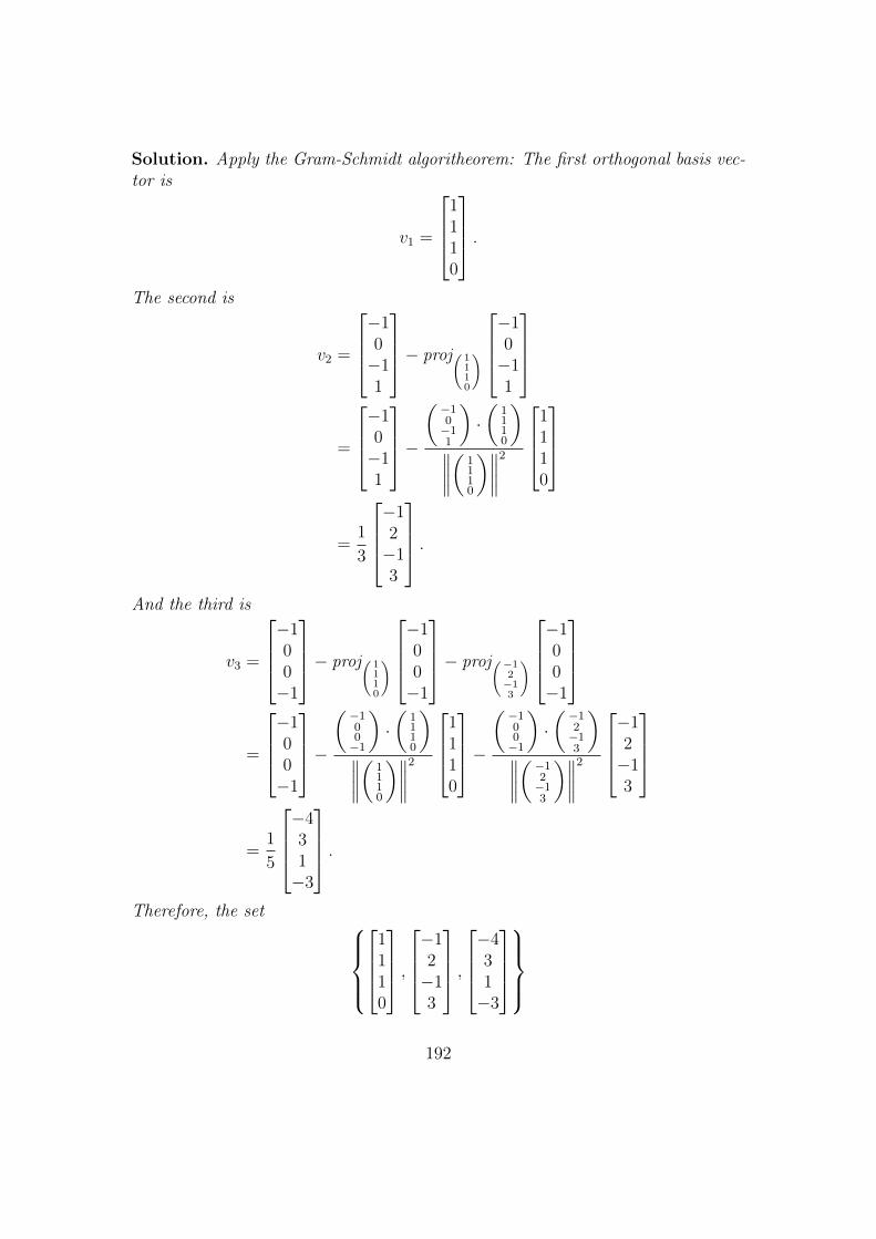
Solution. Apply the Gram-Schmidt algoritheorem: The first orthogonal basis vec-tor is
v1 =
1110
.The second is
v2 =
−10−11
− proj( 1110
)−10−11
=
−10−11
−( −1
0−11
)·(
1110
)∥∥∥∥( 1
110
)∥∥∥∥2
1110
=1
3
−12−13
.And the third is
v3 =
−100−1
− proj( 1110
)−100−1
− proj(−12−13
)−100−1
=
−100−1
−( −1
00−1
)·(
1110
)∥∥∥∥( 1
110
)∥∥∥∥2
1110
−( −1
00−1
)·( −1
2−13
)∥∥∥∥( −12−1
3
)∥∥∥∥2−12−13
=1
5
−431−3
.Therefore, the set
1110
,−12−13
,−431−3
192

is an orthogonal basis for the subspace given in the problem. �
11.5 Application: QR factorization and linear
regression
193

Key concepts from Chapter 11
Definition of orthogonal basis, definition of orthonormal basis, examples oforthogonal and orthonormal bases, orthogonal complements, Theorem 11.9,properties of orthogonal complements, orthogonal projection onto a subspace,properties of orthogonal projection onto a subspace, the Gram-Schmidt algo-rithm.
194

Chapter 12
Singular Value Decomposition
In Chapter 10 we learned that if a square matrix A is orthogonally diagonalizable,then we can understand the transformation TA as a composition of linear scalingsin the directions spanned by the eigenvectors.
12.1 Singular Value Decomposition
12.2 Application: principal component analysis
Suppose that the assignment and test scores of 100 students in a linear algebraclass are recorded into an array in the following way: the students are orderedalphabetically by name, and their scores are recorded into the corresponding row ofan array. If the course had 7 assignments and 3 tests, then the resulting array wouldhave dimensions 100 × 14. For instance, the first row in the array, correspondingto the scores of Arthur Aardvark, might look like this:89 49 61 72 33 99 74 90 89 80
...
195

Appendix A
Extra examples for Chapter 1
In this appendix we provide several additional worked computational examples.
Problem 26 (system with a unique solution). Solve the system
x+ y = 7
x− y = 1.
Solution. Adding the two equations yields
2x = 8 =⇒ x = 4.
Substituting this into either original equation yields y = 3. Therefore, the uniquesolution is (x, y) = (4, 3). �
Problem 27 (System with infinitely many solutions). Solve the system
x+ y = 7 (1)
− 3x− 3y = −21 (2).
Solution. Since equation (2) is −3 times equation (1), if (x, y) solves (1), then italso solves (2), and vice-versa. So, the solutions are
x = t, y = 7− t =⇒ (x, y) = (t, 7− t), t ∈ R.
The set of solutions can be written using set-builder notation as follows.{(t, 7− t) ∈ R2 : t ∈ R
}. �
196

Problem 28 (System with no solutions). Solve the system
x+ y = 4 (1)
2x+ 2y = −4 (2)
Solution. Subtracting 2 times equation (1) from equation (2) yields
0x+ 0y = −12,
which has no solutions. Hence, this system is inconsistent. �
Problem 29. Solve the system
4x1 + x3 = 4
x2 + 3x3 − x5 = 3
x4 + 2x5 = 5.
Solution. The augmented matrix of this system is already in row-echelon form,so we don’t need to perform Gaussian elimination.
The leading variables are x1, x2, and x4. The free variables are x3 and x5.Thus we,
1. Set free variables equal to parameters: x3 = s and x5 = t.
2. Back substitute to solve for leading variables:
x4 + 2t = 5 =⇒ x4 = 5− 2t
x2 + 3s− t = 3 =⇒ x2 = 3 + t− 3s
4x1 + s = 4 =⇒ x1 = 1− s
4.
Therefore, the general form of a solution is
(1− s4, 3 + t− 3s, s, 5− 2t, t)
where t and s are parameters. The solution set is{(1− s
4, 3 + t− 3s, s, 5− 2t, t
)∈ R5 : t, s ∈ R
}. �
197

Problem 30. Solve the system of linear equations
2x1 + x2 − x3 = 1
x1 + x2 + x3 = 6
−3x1 + 2x2 + 4x3 = 13.
Solution. The corresponding augmented matrix is simplified with elementary rowoperations: 2 1 −1 1
1 1 1 6−3 2 4 13
R1↔R2−→
1 1 1 62 1 −1 1−3 2 4 13
R2−2R1−→R3+3R1
1 1 1 60 −1 −3 −110 5 7 31
R3+5R2−→
1 1 1 60 −1 −3 −110 0 −8 −24
.This matrix is in row-echelon form. From this augmented matrix we obtain theequations:
x1 + x2 + x3 = 6
−x2 − 3x3 = −11
−8x3 = −24.
Every variable is a leading variable, so there are no parameters. We solve theseequations by back-substitution. From the third equation, we obtain:
x3 = 3
then we substitute this into the second equation to obtain:
−x2 = −11 + 3(3) = −2 =⇒ x2 = 2.
Finally, substituting these equations into the first equation we obtain:
x1 = 6− (2)− (1) = 1.
Thus there is exactly one solution,
x1 = 1, x2 = 2, x3 = 3.
The set of solutions is {(1, 2, 3)}. �
198

Problem 31. Solve the system
x+ y + z = 6
2x+ y − z = 1
x+ 2y + 4z = 15.
Solution. This system has corresponding augmented matrix1 1 1 62 1 −1 11 2 4 15
.The (1, 1) entry will be used to eliminate the remaining terms in the first column:1 1 1 6
2 1 −1 11 2 4 15
R2−2R1−→R3−R1
1 1 1 60 −1 −3 −110 1 3 9
.Then, using the (2, 2) entry to reduce the matrix to echelon form yields1 1 1 6
0 −1 −3 −110 1 3 9
R3+R2−→
1 1 1 60 −1 −3 −110 0 0 −2
The last row corresponds to the equation 0x+0y+0z = −2, which has no solutions!Thus the system is inconsistent and has no solutions. �
Problem 32. Find the reduced row-echelon form of the matrix1 1 1 60 −1 −3 −110 0 0 −2
.Solution. The solution is given by row reducing. Since the matrix is already inechelon form, all that is left is to use row operations to change the pivots to bothbe 1 and to clear out the remaining terms in the pivot columns. The (2, 1) entryis used to clear out its column and then is changed to be 1:1 1 1 6
0 −1 −3 −110 0 0 −2
R1+R2−→
1 0 −2 −50 −1 −3 −110 0 0 −2
−R2−→
1 0 −2 −50 1 3 110 0 0 −2
.The (3, 4) entry is used to clear its column:1 0 −2 −5
0 1 3 110 0 0 −2
−12R3
−→
1 0 −2 −50 1 3 110 0 0 1
R1+5R3−→R2−11R3
1 0 −2 00 1 3 00 0 0 1
.Note that the pivot columns are all zero except for the pivots. �
199
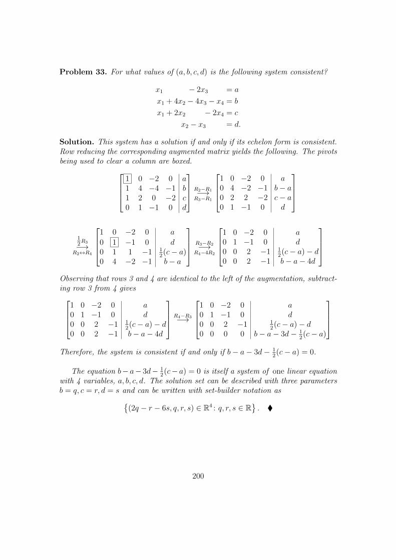
Problem 33. For what values of (a, b, c, d) is the following system consistent?
x1 − 2x3 = a
x1 + 4x2 − 4x3 − x4 = b
x1 + 2x2 − 2x4 = c
x2 − x3 = d.
Solution. This system has a solution if and only if its echelon form is consistent.Row reducing the corresponding augmented matrix yields the following. The pivotsbeing used to clear a column are boxed.
1 0 −2 0 a1 4 −4 −1 b1 2 0 −2 c0 1 −1 0 d
R2−R1−→R3−R1
1 0 −2 0 a0 4 −2 −1 b− a0 2 2 −2 c− a0 1 −1 0 d
12R3
−→R2↔R4
1 0 −2 0 a
0 1 −1 0 d0 1 1 −1 1
2(c− a)
0 4 −2 −1 b− a
R3−R2−→R4−4R2
1 0 −2 0 a0 1 −1 0 d0 0 2 −1 1
2(c− a)− d
0 0 2 −1 b− a− 4d
Observing that rows 3 and 4 are identical to the left of the augmentation, subtract-ing row 3 from 4 gives
1 0 −2 0 a0 1 −1 0 d0 0 2 −1 1
2(c− a)− d
0 0 2 −1 b− a− 4d
R4−R3−→
1 0 −2 0 a0 1 −1 0 d0 0 2 −1 1
2(c− a)− d
0 0 0 0 b− a− 3d− 12(c− a)
Therefore, the system is consistent if and only if b− a− 3d− 1
2(c− a) = 0.
The equation b− a− 3d− 12(c− a) = 0 is itself a system of one linear equation
with 4 variables, a, b, c, d. The solution set can be described with three parametersb = q, c = r, d = s and can be written with set-builder notation as{
(2q − r − 6s, q, r, s) ∈ R4 : q, r, s ∈ R}. �
200

Appendix B
Tutorials
B.1 Tutorial 1: solving systems of linear equa-
tions
In this tutorial we will practice using Gaussian elimination to solve a system oflinear equations and describing the set of solutions. We will also check our under-standing of some terminology and finish the proof of Theorem 1.13 in the lecturenotes.
Background: Chapter 1. If you have forgotten the definition of a word in thisworksheet, try looking it up in the index.
1. Consider the following system of linear equations in the variables x1, x2, x3, x4, x5.
3x1 + 2x2 + x5 = 4 + x3
x2 = 4 + x4
+x3 = 5 + x1 + x2 + 3x4
(a) Write the augmented matrix for this system and use Gaussian elimina-tion to put the matrix in row-echelon form.
(b) What is the reduced row-echelon form of the coefficient matrix?
(c) What is the rank of the coefficient matrix for this system?
(d) Use the result from part (a) to describe the set of solutions to thissystem of linear equations.
(e) Is the system consistent or inconsistent?
201

(f) How many solutions does this system of linear equations have? Relateyour answer to part (c).
2. Give examples of systems of linear equations in three variables (call them x,y, and z) with each of the following properties, or explain why no exampleexists. Justify your answers.
(a) A system with exactly one solution, (1, 1,−1).
(b) A system that is inconsistent.
(c) A system with infinitely many solutions, such that the solutions satisfythe equation x+ y = z.
(d) A system with exactly four solutions.
(e) A system whose augmented matrix has rank 2.
(f) A system whose augmented matrix has rank 0.
(g) A system whose augmented matrix has rank 4.
(h) A system whose augmented matrix has rank 5.
3. Suppose that a, b, c, d, e, and f are numbers and
ax+ by = e
cx+ dy = f
is a system of linear equations in the variables x and y.
(a) Prove that if (x0, y0) and (x1, y1) are solutions to this system, then forevery real number t ∈ R, the pair
(tx1 + (1− t)x0, ty1 + (1− t)y0)
is a solution.
(b) Use part (a) to explain why a 2× 2 system of linear equations can onlyhave 0 solutions, 1 solution or infinitely many solutions.
(c) Your answer to part (b) is a proof of Theorem 1.13 for the special case oftwo equations in two variables. Can you adapt this proof to the generalcase (m equations in n variables)?
202

4. The second elementary operation on systems of linear equations is “multiplyan equation by a non-zero number.” Why is it not “multiply an equation bya number”?
5. Suppose that the rank of the augmented matrix [A|b] of an inconsistent sys-tem of linear equations is r. What is the rank of the coefficient matrix A?
What if the system of linear equations is consistent?
6. (food for thought) In class we learned that the important feature of elemen-tary operations on a system of linear equations is Theorem 1.18: they do notchange the set of solutions of the system.
Of course, we can define many other ‘operations’ on systems of linear equa-tions that are not elementary operations. For each of the following operationson systems of equations, discuss whether it will change the set of solutions.You may want to try the operations on some simple examples.
For simplicity, suppose we are only discussing systems of linear equations inthree variables, x1, x2, x3.
(a) Add a new equation to the system of linear equations.
(b) Delete an equation from the system of linear equations.
(c) Multiply the coefficient of x1 in each equation by 5.
(d) In each equation, switch the coefficients of x1 and x3. For example,
x1 − 2x2 + 5x3 = 0→ 5x1 − 2x2 + x3 = 0.
(e) Replace the constant terms in each equation with 0.
(f) In each equation, add the coefficient of x1 to the coefficient of x2. Forexample,
x1 − 2x2 + x3 = 0→ x1 − x2 + x3 = 0.
(g) In each equation, set x3 = 1.
B.2 Tutorial 2: matrix algebra
In this tutorial we will explore matrix algebra, with a focus on the comparison withhighschool algebra.
203

Background: Highschool algebra and material from Chapter 2.
1. Suppose that A is a 2 × 3 matrix, B is a 3 × 2 matrix, u is a 3 × 1 columnvector, and w is a 1 × 3 row vector. Which the following expressions areequal? Justify your answers using properties of matrix algebra.
(i) uw(B − AT )
(ii) wTuT(B − AT
)(iii) −
(AwTuT −BTwTuT
)T(iv) (BTuw)T − (uw)TAT
(v) BBT
(vi) BTB
2. Suppose A is the 2× 2 matrix
A =
[1 11 0
]Find all 2× 2 matrices B that solve the matrix equation
AB = BA.
Use set-builder notation to describe your final answer.
Hint: Convert the matrix equation into a system of linear equations. Solvethe system of equations. Convert your answer back into a matrix.
3. Consider the following list of algebraic identities and facts that are true whenx, y, and z are real numbers.
(a) x+ y = y + x
(b) xy = yx (hint: compare this equation with question 2)
(c) If xy = xz and x 6= 0, then y = z.
(d) x2 + 2xy + y2 = (x+ y)2
(e) x2y2 = xyxy
(f) x2 ≥ 0
204

(g) If x2 = 1, then x = ±1. (compare with your answer to question 4).
(h) If xy = 0, then x = 0 or y = 0.
Which of these algebraic identities/facts are true if the numbers x, y, andz are replaced with matrices A,B, and C? Be careful to specify what thenumber of rows and columns of the matrices must be in order for the equa-tions to make any sense.
For example: for part (a), the corresponding equation with matrices isA + B = B + A. For this equation to make sense, A and B must bothhave the same number of rows and columns. Is this equation always true forany m× n matrices? Can you cite a fact from class?
If the identity for matrices is true, explain why. If it is not true, give anexample that demonstrates it is false.
4. We know from highschool algebra that the roots of a quadratic polynomialp(x) = ax2 + bx+ c are given by the formula
x =−b±
√b2 − 4ac
2a.
Using matrix multiplication, addition, and scalar multiplication, we can writean analogous matrix equation for n× n matrices X, and scalars a, b, and c,
aX2 + bX + cIn = 0.
Here In is the n×n identity matrix and 0 is the n×n zero matrix. Althoughthese matrix equations look like quadratic polynomials, the set of solutionsis very different.
(a) Can you find some or all solutions to the matrix equation X2 − I = 0when X is a 2 × 2 matrix? How does your answer compare to thesolutions to the equation x2 − 1 = 0? Describe your answer with set-builder notation.
(b) Is it possible to use Gaussian elimination to find the set of all solutionsto the matrix equation in part (a)?
205

We know from highschool that the quadratic polynomial p(x) = ax2 + bx+ conly has real roots if the discriminant ∆ := b2−4ac is a non-negative number(∆ ≥ 0). For example, the descriminant of the polynomial
q(x) = x2 + 1
is ∆ = −4 and q(x) has no real roots.
Suppose X is a 2× 2 matrix. Unlike q(x) = 0, the matrix equation
X2 + I = 0
does have solutions!
(c) Find all solutions of the matrix equation X2 + I = 0. How does youranswer compare to the set of solutions of the equation x2 + 1 = 0? Useset-builder notation to describe your answer.
5. A square matrix A = [aij]n×n is called upper triangular if
aij = 0 when i > j.
(i) Write down the general form of a 2 × 2 and 3 × 3 upper triangularmatrix.
(ii) Show that the product of two upper-triangular matrices is upper-triangular.(Hint: try the cases n = 2, 3 first, then see if you can make your argu-ment general).
6. A matrix A is called purple1 if A = AT . For each of the following statements,say whether it is true or false. Justify your answers with an explanation.
(i) The matrix
A =
1 11 00 0
is purple.
1The real word for this property is symmetric.
206
(ii) The matrix
A =
[1 11 0
]is purple.
(iii) The matrix
A =
[1 01 0
]is purple.
(iv) If A is a purple matrix, then A is a square matrix.
(v) If A and B are purple n× n matrices, then A+B is purple.
(vi) If A and B are purple n× n matrices, then 3A+ 8BT is purple.
(vii) If B is a m× n matrix, then BBT is a purple m×m matrix and BTBis a purple n× n matrix.
(viii) If A is a purple matrix, then A2 is a purple matrix.
(ix) If A is a purple matrix, then A3 is a purple matrix.
(x) If A and B are purple n× n matrices, then AB is purple.
(xi) If A and B are n× n matrices and B is purple, then ABA is purple.
(xii) If A and B are n× n matrices and B is purple, then ABAT is purple.
7. (food for thought) Operations on matrices effect their rank in interestingways. Here are some questions to think about (we will return to them laterin the course, after test 1).
For each item below, suppose A and B are matrices so that the operationsmake sense.
(i) What is the relation between rank(A) and rank(AT )?
(ii) What is the relation between rank(A), rank(B) and rank(A+B)?
(iii) What is the relation between rank(A), rank(B) and rank(AB)?
For each of these questions, you can explore what is true by trying out vari-ous examples with different A and B.
In the following two questions, we explore some matrix operations other thanthe ones introduced in chapter 2. These operations have their own interestingproperties and are useful in many applications. Let’s explore these opera-tions.
207
8. If A and B are matrices with the same dimension n×m, then we can definethe element-wise multiplication A ∨ B (this notation is not standard) to bethe n×m matrix whose i, jth entry is simply ai,jbi,j.
(i) Compute the element-wise multiplication of
A =
0 13 40 9
and
B =
1 11 −13 0
.(ii) What properties does element-wise multiplication have? For instance,
is it always true that A∨B = B∨A? Is it always true that A∨(B+C) =A ∨ B + A ∨ C (provided the operations are defined)? Can you thinkof other properties to check?
(iii) Describe the differences between matrix multiplication AB and element-wise matrix multiplication A ∨B.
(iv) If A is a square matrix, then you can compute A ∨ A. What can yousay about the matrix A ∨ A?
B.3 Tutorial 3: More systems of linear equations
In this tutorial we will practice: using matrix algebra to study systems of linearequations, and determining whether a vector is contained in a span.
Background: Chapter 3 of the lecture notes.
1. (warm-up) Compute the basic solutions of the following homogeneous systemof equations.
3x1 + 2x2 + x5 = x3
x2 = x4
x3 = x1 + x2 + 3x4
208

Compare your answer with Problem 1 from Tutorial 1. Write the solutionsto Problem 1 from Tutorial 1 as the sum of a particular solution plus ahomogeneous solution.
2. Suppose A is a 2 × 4 matrix and u =
1100
and v =
1011
are basic
solutions of the homogeneous system Ax = 0.
Are the follow statements true or false? Justify your answers.
(i)
0−111
is a solution.
(ii)
6333
is a solution.
(iii)
1000
is a solution.
(iv) There are 3 basic solutions.
(v) There are 2 basic solutions.
(vi) The rank of A is 2.
(vii) Every solution is a linear combination of u and v.
3. Use matrix algebra to prove the following theorem.
Theorem: Suppose that u1, . . .uk are solutions of the matrixequation Ax = b. If t1, . . . , tk are real numbers such that
t1 + t2 + · · ·+ tk = 1,
then the linear combination
t1u1 + t2u2 + · · ·+ tkuk
is a solution of the matrix equation Ax = b.
209
Once you are done proving this theorem, go back and use this result toanswer question 3 in tutorial 1 again.
5. Suppose u and v are m×1 column vectors. Which of the following statementsare always true? Justify your answers.
(i) 0m×1 ∈ span {u,v}(ii) u ∈ span {u,v}(iii) 2u− v ∈ span {u,v}(iv) 2u− v ∈ span {2u− v,u + v}(v) u ∈ span {u + v, 2u + 2v}(vi) b ∈ span {u,v} for every m× 1 column vector b.
Suppose A is a m× 2 matrix with columns u and v as above. Which of thefollowing statements are always true? Justify your answers.
(i) The homogeneous system Ax = 0 is consistent.
(ii) The system Ax = u is consistent.
(iii) The system Ax = 2u− v is consistent.
(iv) The system Ax = u + v is consistent.
(v) The system Ax = b is consistent for every m× 1 column vector b.
(vi) The system Ax = u + b is consistent for every m× 1 column vector b.
B.4 Tutorial 4: Matrix inverses
In this tutorial we will practice finding matrix inverses, using the big theorem forsquare matrices, and using properties of matrix inverses.
Background: Chapter 4 of the lecture notes.
1. (warm-up) For each of the following matrices, determine whether the matrixis invertible and, if it is invertible, find its inverse.
A =
1 0 12 1 11 1 1
, B =
1 0 12 1 11 0 1
210

If the matrix is invertible, write the matrix and its inverse as a product ofelementary matrices.
2. Consider a homogeneous system of two equations in the variables x1, x2 witharbitrary coefficients a, b, c, d,
ax1 + bx2 = 0
cx1 + dx2 = 0
For what values of a, b, c, d does this system have exactly one solution? Givea complete explanation of your answer.
3. Definition: A square matrix A is called orange2 if
ATA = I and AAT = I.
(i) Which elementary matrices are orange?
(ii) Find two examples of orange matrices that aren’t elementary matrices(hint: try products of elementary matrices).
(iii) Is the identity matrix orange? Why?
(iv) A orange matrix is always invertible. What is the inverse?
(v) Show that if A is orange, then AT is orange.
(vi) Show that the product of two n× n orange matrices is orange.
4. Suppose that A is a n× n matrix such that Ax = b has a solution for everyb ∈ Rn. Which of the following statements are true? Explain your answer.
(i) A is invertible.
(ii) Ax = 0 is consistent.
(iii) The span of the columns of A is Rn.
(iv) There are elementary matrices E1, . . . , Ek such that Ek · · ·E1A = I.
(v) AT is invertible.
(vi) The span of the columns of AT is Rn.
(vii) The equation A−1x = b has a unique solution for every b ∈ Rn.
(viii) The rank of A is n.
2The real word for this property is orthogonal.
211

(ix) A3 is invertible.
5. Use the Big Theorem for Square Matrices to prove the following statement.
If A is invertible, then A does not have a row of zeros.
On the other hand, consider the following statement:
If A does not have a row of zeros, then A is invertible.
Is this statement true?
Hint: Look at your results from the warm-up.
6. In this question A and B are n× n matrices.
(i) Show that if AB is invertible, then B is invertible.
Warning: Be careful that your logic is not circular. If you write B−1
in your proof, then you have implicitly assumed B is invertible whiletrying to explain why B is invertible.
(ii) Suppose that A is invertible and AB is not invertible. Explain why Bcannot be invertible.
(iii) Use part (b) to complete the proof from the section on the matrixinversion algorithm. Show that if E1, . . . , Ek are elementary matrices,and Ek · · ·E2E1A is not invertible, then A is not invertible.
7. (bonus) Suppose that A is an invertible n × n matrix and u,v are nonzeron× 1 column vectors.
(i) The Sherman-Morrison formula says that if 1 + vTA−1u 6= 0, thenA+ uvT is invertible and the inverse is given by the formula
(A+ uvT )−1 = A−1 − 1
1 + vTA−1uA−1uvTA−1.
Verify the Sherman-Morrison formula.
This formula is used in many applications for quickly computing inversesof large matrices: If you have a matrix C = A+B where A is a matrixwhose inverse you can easily compute (maybe A is a diagonal matrix,
212

for example) and B is a matrix of rank 1 (i.e. B = uvT ), then theSherman-Morrison formula gives you a fast way to compute the inverseof C.
(ii) Suppose that 1 + vTA−1u = 0. Is A + uvT invertible? Justify youranswer.
B.5 Tutorial 5: Vector geometry
Background: Chapter 5 of the lecture notes.
1. (i) Find the equation of the plane that contains the points
(2, 4, 4), (2,−2, 2), (4, 2, 2) ∈ R3.
(ii) Find the equation of the plane that contains the points
(2, 1, 3), (3, 0, 2), (3, 3, 3) ∈ R3.
(iii) Show that the two planes from part (a) and part (b) are the same.
(iv) (food for thought) What trick did I use come up with the three pointsfor part (b) using the three points from part (a) so that I knew the twoplanes would be the same without having to check?
2. (i) Show that the three points
P0 = (5, 6, 1), P1 = (−1,−2, 3), P2 = (11, 14,−1)
are collinear.
(ii) Describe all the planes that contain all three points, P0, P1, P2 (thereare infinitely many).
Hint: use normal vectors.
3. (i) Show that if two vectors u,v ∈ Rn are parallel, then
projuv = v.
(ii) Show that if u,v ∈ Rn are orthogonal, then
projuv = 0.
213

(iii) Show that for any vectors u,v ∈ Rn,
||projuv|| ≤ ||v||.
Hint: Use the definition of projuv and properties of the dot-product.
4. Show that for any two vectors, u = [u1 u2 u3] and v = [v1 v2 v3], the vector
x = u× v
is a solution of the matrix equation[u1 u2 u3v1 v2 v3
]x = 0.
5. Three points, P0, P1, P2 ∈ R3 are called collinear if they all lie on the sameline.
(i) Are the points (0, 0, 0), (1, 0, 0), (−10, 0, 0) collinear?
(ii) Are the points (0,−1, 4), (0,−1, 7), (0,−1, 10) collinear?
(iii) Are the points (2, 0, 0), (0, 1, 0), (0, 0, 1) collinear?
(iv) Show that the following two statements are equivalent:
• P0 = (x0, y0, z0), P1 = (x1, y1, z1), P2 = (x2, y2, z2) are collinear.
• There is a number t ∈ R such that
x2 = tx1 + (1− t)x0y2 = ty1 + (1− t)y0z2 = tz1 + (1− t)z0
Hint: use the fact that a point and a vector determine a line.
(v) Use part (d) to show that if P0, P1, P2 are collinear, then the matrix x0 y0 z0x1 y1 z1x2 y2 z2
has rank ≤ 2.
214
(vi) Compute the rank of the matrix from part (e) for the three points fromparts (a)-(c).
6. Consider the two vectors
u =
12−1
,v =
011
(i) Show that u and v are not parallel.
(ii) Write the equation of the plane through the origin determined by thevectors u and v (use the cross-product to find a normal vector).
(iii) Show that the plane through the origin determined by the vectors uand v equals the set
span{u,v}.
This has two steps:
• Show that any linear combination tu+sv is a solution to the equa-tion from part (b).
• Show that any point that solves the equation from part (b) can bewritten as a linear combination tu + sv.
7. Let Q1 = (1,−1) and Q2 = (−1, 1). Describe the set of points P = (x, y)such that
d(P,Q1) = d(P,Q2).
215

8. (bonus) The area of a parallelogram in R2 with adjacent sides u and v canbe computed with the formula
Area = ||u||||v|| sin(θ)
where θ is the angle between u and v.
Use this formula and other properties of angles and dot products to show
that if u =
[ac
]and v =
[bd
], then
Area = ad− bc.
One approach: we know Area2 = ||u||2||v||2 sin2(θ) = ||u||2||v||2(1−cos2(θ)).Plug in formulas and simplify.
B.6 Tutorial 6: Linear transformations
Background: Chapter 6 of the lecture notes.
1. Suppose that
u =
121
, v =
101
, w =
110
.Let T be the linear transformation such that
T (u) =
100
, T (v) =
010
, T (w) =
001
.(i) Use properties of linear transformations to find the matrix of T .
Hint: first, write the standard basis vectors e1, e2, e3 as linear combi-nations of u,v,w. Second, use properties of linear transformations tocompute the vectors T (e1), T (e2), T (e3).
(ii) This linear transformation is invertible. Use the matrix from part (a)to compute the matrix of T−1.
216

(iii) There is another (quicker) way to find the matrix of T−1 without usingthe matrix from part (a). What is it?
2. Consider two linear transformations of R2,
Tθ
([xy
])=
[cos(θ) − sin(θ)sin(θ) cos(θ)
] [xy
]F
([xy
])=
[−1 00 1
] [xy
]The transformation Tθ rotates R2 by an angle of θ in a counterclockwisedirection. The transformation F reflects points in R2 about the y-axis.
(i) Consider the three vertices of a triangle, P0 = (1, 0), P1 = (−1, 1) andP2 = (−1,−1).
When θ = π/2, Tπ/2 describes a counter-clockwise rotation of R2 by anangle of π/2.
For all three points, P0, P1, P2, compute
Tπ/2(P0), Tπ/2(P1), Tπ/2(P2).
Illustrate your computation by drawing the three points, and their im-age under Tπ/2 in R2.
Draw a picture of the image of the triangle under Tπ/2.
(ii) For all three points, P0, P1, P2, compute
F (P0), F (P1), F (P2).
Illustrate your computation by drawing the three points, and their im-age under F in R2.
Draw a picture of the image of the triangle under F
217

(iii) We can compose F and Tπ/2 two ways.
For all three points, P0, P1, P2, compute their image under the transfor-mation F ◦ Tπ/2. Draw a picture of the result.
For all three points, P0, P1, P2, compute their image under the transfor-mation Tπ/2 ◦ F . Draw a picture of the result.
(iv) Compare the two pictures from part (c). Does F ◦ Tπ/2 = Tπ/2 ◦ F?
3. For each item below, give an example of a linear transformation with thatproperty or explain why no linear transformation with that property exists.
(i) T is injective and surjective.
(ii) T is injective but not surjective.
(iii) T is surjective but not injective.
(iv) T : R3 → R3 is invertible.
(v) T : R3 → R3 is invertible but not injective.
(vi) T : R3 → R3 is injective but not surjective
(vii) For every nonzero vector x, T (x) 6= x and T ◦ T (x) = x.
Hint: can you think of a matrix A 6= I so that A2 = I?
(viii) T : R3 → R3 and the image of T is span{[1 5 2]T}.(ix) T : R→ R3 and the image of T is span{[1 5 2]T}.(x) T : R2 → R3 and the image of T is span{[1 5 2]T}.
4. Given a column vector u =
u1...un
∈ Rn.
We know that uTu is a number, and uuT is a n× n matrix.
218

(i) Use the definition of the orthogonal projection projux to show thatthe matrix of the linear transformation T (x) = projux is given by theformula
A =1
uTuuuT .
(ii) Use the result from part (a) to compute the matrix of the orthogonal
projection proju : R3 → R3 for the vector u =
−121
.
(iii) For the orthogonal projection in part (b), write the sets ker(proju) andim(proju) as the span of a set of vectors.
(iv) Use the result from part (a), and properties of matrix algebra, to showthat the matrix A of orthogonal projection onto a line is always purple(Remember, A is purple if A = AT ).
5. A linear transformation T : Rn → Rn is called covfefe if for every vectorx ∈ Rn,
||T (x)|| = ||x||.
(i) Which of the following linear transformations R2 → R2 are covfefe?
i. Rotation by θ degrees.
ii. Reflection through a coordinate axis.
iii. Scaling (dilation) by a factor of k.
iv. The shear transformation with matrix[1 a0 1
].
v. Orthogonal projection onto a line through the origin.
(ii) Describe in words what a covfefe transformation does geometrically.
(iii) Recall that a square matrix A is called orange if AAT = ATA = I.Show that if A is orange, then the linear transformation TA(x) = Ax iscovfefe.
(iv) Show that if a linear transformation T is covfefe, then ker(T ) = {0}.(v) Use the result of part (d) and the Theorems from section 6.9 of the
lecture notes to explain why every covfefe linear transformation is in-vertible.
219
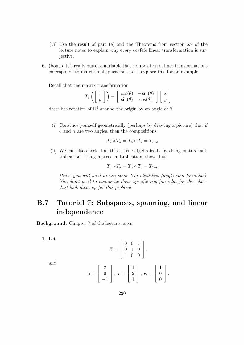
(vi) Use the result of part (e) and the Theorems from section 6.9 of thelecture notes to explain why every covfefe linear transformation is sur-jective.
6. (bonus) It’s really quite remarkable that composition of liner transformationscorresponds to matrix multiplication. Let’s explore this for an example.
Recall that the matrix transformation
Tθ
([xy
])=
[cos(θ) − sin(θ)sin(θ) cos(θ)
] [xy
]describes rotation of R2 around the origin by an angle of θ.
(i) Convince yourself geometrically (perhaps by drawing a picture) that ifθ and α are two angles, then the compositions
Tθ ◦ Tα = Tα ◦ Tθ = Tθ+α.
(ii) We can also check that this is true algebraically by doing matrix mul-tiplication. Using matrix multiplication, show that
Tθ ◦ Tα = Tα ◦ Tθ = Tθ+α.
Hint: you will need to use some trig identities (angle sum formulas).You don’t need to memorize these specific trig formulas for this class.Just look them up for this problem.
B.7 Tutorial 7: Subspaces, spanning, and linear
independence
Background: Chapter 7 of the lecture notes.
1. Let
E =
0 0 10 1 01 0 0
.and
u =
20−1
, v =
121
, w =
100
.220

(i) Compare the subspaces S = span{u} and S ′ = span{Eu}.(ii) Compare the subspaces S = span{v} and S ′ = span{Ev}.(iii) Compare the subspaces S = span{u,v} and S ′ = span{Eu, Ev}.(iv) Compare the subspaces S = span{u,w} and S ′ = span{Eu, Ew}.(v) Compare the subspaces S = span{u,v,w} and S ′ = span{Eu, Ev, Ew}.
2. Which of the following sets are subspaces of R2? Justify your answer. Drawa picture of what the set looks like.
(i) A line.
(ii) A point.
(iii) A circle of radius 2 centred at (0, 2).
(iv) R2.
(v) The set of points equidistant from (1, 1) and (−1,−1).
(vi) The set of points {(x, y) ∈ R2 : y = x2}.(vii) The set of points {(x, y) ∈ R2 : x ≥ 0}.(viii) The set of points {(x, y) ∈ R2 : x2 ≥ 0}.
3. True or false.
(i) If S is a subspace of Rn, then dim(S) < n.
(ii) If S is a subspace of Rn, then dim(S) > 0.
(iii) If {u,v} is a set of two vectors in R3, then there is a vector w so that{u,v,w} is a basis for R3.
(iv) If {u,v,w,x} is a set of vectors in R3, then it is linearly dependent.
(v) If 0 is not contained in a set of vectors U , then U is linearly independent.
(vi) If S and S ′ are subspaces of Rn with dim(S) = dim(S ′), then S = S ′.
4. Suppose S is a set of points in Rn and T : Rn → Rm is a linear transformation.
Define the setS ′ = {T (x) : x ∈ S} ⊆ Rm.
We call S ′ the image of S under T .
221
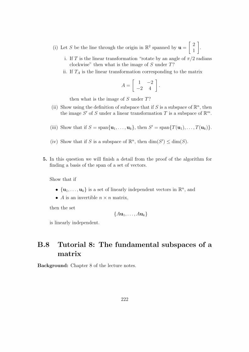
(i) Let S be the line through the origin in R2 spanned by u =
[21
].
i. If T is the linear transformation “rotate by an angle of π/2 radiansclockwise” then what is the image of S under T?
ii. If TA is the linear transformation corresponding to the matrix
A =
[1 −2−2 4
].
then what is the image of S under T?
(ii) Show using the definition of subspace that if S is a subspace of Rn, thenthe image S ′ of S under a linear transformation T is a subspace of Rm.
(iii) Show that if S = span{u1, . . . ,uk}, then S ′ = span{T (u1), . . . , T (uk)}.
(iv) Show that if S is a subspace of Rn, then dim(S ′) ≤ dim(S).
5. In this question we will finish a detail from the proof of the algorithm forfinding a basis of the span of a set of vectors.
Show that if
• {u1, . . . ,uk} is a set of linearly independent vectors in Rn, and
• A is an invertible n× n matrix,
then the set{Au1, . . . , Auk}
is linearly independent.
B.8 Tutorial 8: The fundamental subspaces of a
matrix
Background: Chapter 8 of the lecture notes.
222

1. Let
A =
1 −2 0 0 32 −5 −3 −2 60 5 15 10 02 6 18 8 6
The reduced row echelon form of A is
R =
1 −2 0 0 30 1 3 2 00 0 1 1 00 0 0 0 0
(i) What is the rank of A?
(ii) Find a basis for null(A). What is the nullity of A?
(iii) Find a basis for col(A). What is the dimension of the column space of A?
(iv) Find a basis for row(A). What is the dimension of the row space of A?
(v) Check the rank-nullity theorem for A.
(vi) Write a basis for the column and row space of AT .
(hint: the rows of A are the columns of AT and vis versa)
(vii) What is the rank of AT ? Why?
(It’s important to note that you know the rank of AT without havingto row-reduce AT )
(viii) What is the dimension of the null space of AT ?(It’s important to note that you can answer this question without find-ing a basis for the null space of AT )
2. In this question we will explore examples and theory related to Theorem 8.9in the lecture notes.
223

(i) Are the statements in Theorem 8.9 true for the matrix
A =
1 −22 −50 52 6
?
(ii) Are the statements in Theorem 8.9 true for the matrix
A =
[1 −2 12 −5 0
]?
(iii) Are the statements in Theorem 8.9 true for the matrix
A =
[1 72 −5
]?
(iv) Is it possible for any of the statements in Theorem 8.9 to be true for amatrix with fewer rows than columns (m < n)? Why?
(v) Use the result from part (d) to explain the following fact.
Fact: If A is a m× n matrix and m < n, then the matrix equation
XA = In
has no solutions (i.e. there is no n×m matrix X that solves this equa-tion). In other words, A cannot have a left inverse.
(vi) Give an example of a 4× 3 matrix A such that every statement in The-orem 8.9 is false for A.
(vii) Give an example of a linear transformation T : R3 → R4 that is notinjective.
3. In this question we will explore examples and theory related to Theorem 8.11in the lecture notes.
(i) Are the statements in Theorem 8.11 true for the matrix
A =
1 −22 −50 52 6
?
224

(ii) Are the statements in Theorem 8.11 true for the matrix
A =
[1 −2 12 −5 0
]?
(iii) Are the statements in Theorem 8.11 true for the matrix
A =
[1 72 −5
]?
(iv) Is it possible for any of the statements in Theorem 8.9 to be true for amatrix with fewer columns than rows (n < m)? Why?
(v) Use the result from part (d) to explain the following fact.
Fact: If A is a m× n matrix and n < m, then the matrix equation
AX = Im
has no solutions (i.e. there is no n×m matrix X that solves this equa-tion). In other words, A cannot have a right inverse.
(vi) Give an example of a 3× 4 matrix A such that every statement in The-orem 8.11 is false for A.
(vii) Give an example of a linear transformation T : R4 → R3 that is notsurjective.
4. In this question we will explore how matrix multiplication effects the nullspace and rank of a matrix.
The proofs of the theorems at the end of this question are bonus exercises,but the statements of the theorems are something that everyone should know.
(i) Consider the matrices
A =
[1 −11 1
], B =
[1 −2 01 1 1
]
225

Compute a basis for null(B) and null(AB). Use the result of yourcomputation to explain that
null(B) = null(AB).
(ii) Consider the matrices
A =
[1 11 1
], B =
[1 −2 01 1 1
]Compute a basis for null(B) and null(AB). Use the result of yourcomputation to explain that
null(B) ⊆ null(AB).
but the two subspaces are not equal.
(iii) Show that, in general, if A is a m× n matrix and B is a n× p matrix,then
null(B) ⊆ null(AB).
Hint: You simply need to show that every element of null(B) is an ele-ment of null(AB). In order to do this, you need to use the definition of“null space” and a simple matrix algebra argument.
(iv) (bonus) Use part (c) and the rank-nullity theorem to conclude the fol-lowing theorem:
Theorem: If A is a m× n matrix and B is a n× p matrix, then
rank(B) ≥ rank(AB).
(v) There is a similar but slightly different fact:
Theorem: If C is a n×m matrix and D is a p× n matrix, then
rank(D) ≥ rank(DC).
(bonus) Prove this theorem.
Hint: Although this theorem is different from the previous one, you canuse the previous one to prove it. Look at the theorem from the previousquestion. Use the fact that taking transposes does not change rank, butit does change the order of multiplication.
226

(vi) In part (a), we saw an example where A was invertible and we observedthat null(B) = null(AB).
In fact, this is true in general:
Theorem: If A is an invertible n× n matrix and B is a n× p matrix,then
null(B) = null(AB).
(bonus) Prove this theorem.
Hint: By the result from part (c), we know that null(B) ⊆ null(AB).To show that null(AB) ⊆ null(B), use the fact that the homogeneoussystem Ax = 0 has a unique solution when when A is invertible.
Here is a hint for a different, slightly more complicated proof.
Hint for proof 2: First, use the fact that A can be written as a productof elementary matrices to explain why the rank of A and AB must bethe same. Second, combine the rank-nullity theorem, the result frompart (c), and Theorem 7.12(g) from the lecture notes.
B.9 Tutorial 9: Determinants
Background: Chapter 9 of the lecture notes.
1. (warm-up) Use cofactor expansion to compute the determinant of the fol-lowing matrices.
(i) A =
[1 20 3
].
(ii) B =
1 4 26 1 −13 1 1
.
227
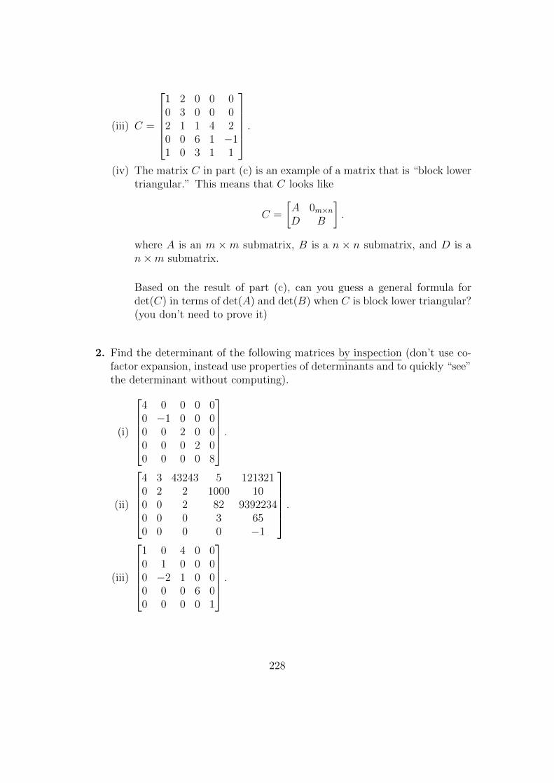
(iii) C =
1 2 0 0 00 3 0 0 02 1 1 4 20 0 6 1 −11 0 3 1 1
.(iv) The matrix C in part (c) is an example of a matrix that is “block lower
triangular.” This means that C looks like
C =
[A 0m×nD B
].
where A is an m ×m submatrix, B is a n × n submatrix, and D is an×m submatrix.
Based on the result of part (c), can you guess a general formula fordet(C) in terms of det(A) and det(B) when C is block lower triangular?(you don’t need to prove it)
2. Find the determinant of the following matrices by inspection (don’t use co-factor expansion, instead use properties of determinants and to quickly “see”the determinant without computing).
(i)
4 0 0 0 00 −1 0 0 00 0 2 0 00 0 0 2 00 0 0 0 8
.
(ii)
4 3 43243 5 1213210 2 2 1000 100 0 2 82 93922340 0 0 3 650 0 0 0 −1
.
(iii)
1 0 4 0 00 1 0 0 00 −2 1 0 00 0 0 6 00 0 0 0 1
.
228

(iv)
0 1 0 0 01 0 0 0 00 0 0 1 00 0 1 0 00 0 0 0 1
.
(v)
0 0 0 0 10 1 0 0 00 0 100 0 00 0 0 1 01 0 0 0 0
.
(vi)
0 0 0 0 10 0 0 0 00 0 100 0 00 0 0 1 01 0 0 0 0
.
3. Suppose that A and B are 3×3 matrices with det(A) = −1 and det(B) = 2.Compute each of the following determinants using properties of the determi-nant.
(i) det(2A2)
(ii) det(A3B5)
(iii) det(BABABAB2)
(iv) det(3A2B−1)
(v) det(3(A2B−1)T )
4. Consider the matrix
A =
[1 2 01 0 3
].
(i) Compute det(AAT )
(ii) Compute det(ATA)
(iii) Here is a fake proof that det(AAT ) = det(ATA) (which we know is falseby our computations in part (a) and (b)). Try to explain the mistakein this fake proof.
229

Fake proof: We show that det(AAT ) = det(ATA) using properties ofdeterminants.
det(AAT ) = det(A) det(AT ) since det(AB) = det(A) det(B)
= det(AT ) det(A) since the order of multiplying two numbers doesn’t matter
= det(ATA) since det(AB) = det(A) det(B)
(iv) (food for thought) The computations from part (a) and (b) tell us thatone of the matrices AAT and ATA is invertible, but the other is not.Can you relate this to Theorems 8.9 and 8.11 in the lecture notes?
B.10 Tutorial 10: Eigenvalues, eigenevectors,
and diagonalization
Background: Chapter 10 of the lecture notes.
1. (warm-up) Compute the eigenvalues and corresponding eigenspaces for thematrices below.
[7 4−3 −1
],
[4 −2−3 9
],
4 2 3−1 1 −32 4 9
, 4 0 0−1 4 −30 0 1
.Which of the matrices are diagonalizable? For each matrix that is diagonal-izable, compute its diagonalization.
2. In this question we explore an application of matrix diagonalization: com-puting large powers of a matrix3
3Computing the matrix product AB (where A and B are n×n matrices) using the definitionof matrix multiplication is an algorithm that takes an order of n3 operations (one is countedevery time you add, multiply two numbers together). For instance, if you try to computeA1000, and A is a 10 × 10 matrix, you will use roughly 1, 000, 000 operations. However, if A isdiagonalized, you only need to compute powers of diagonal entries, which is much faster.
It is interesting to note that there are clever algorithms for matrix multiplication that are moreefficient than the definition when taking products of large matrices (even if the matrices aren’tdiagonalizable). See the Strassen algorithm on wikipedia.
230

(i) If A = PDP−1, then there is a simple formula for Ak (where k is apositive integer). What is it?
(ii) For each of the matrices from question 1 that are diagonalizable, useformula from part (a) to compute A2017 (you don’t need to simplifypowers of numbers that appear in your final answer).
3. Suppose that A and B are 3×3 matrices. Which of the following statementsare true or false, and why?
(i) If −2 is an eigenvalue of A, then −8 is an eigenvalue of A3.
(ii) If −2 is an eigenvalue of A, then −8 is an eigenvalue of 2A3.
(iii) If −2 is an eigenvalue of A and −2 is an eigenvalue of B, then 4 is aneigenvalue of AB.
(iv) If −2 is an eigenvalue of A and −2 is an eigenvalue of B, then −2 is aneigenvalue of A+B.
(v) If A2 = I, then the only eigenvalues of A are 1 or -1.
(vi) If A2 = A, then the only eigenvalues of A are 1.
(vii) If A has two distinct eigenvalues, then A is diagonalizable.
(viii) If A is invertible, then A is diagonalizable.
4. In this question we will add another fact to our list of equivalent statementsfor n× n matrices.
Theorem Suppose that A is a n× n matrix. The following two statementsare equivalent.
(i) A is invertible.
(ii) 0 is not an eigenvalue of A.
Hint: use the characteristic polynomial, and the list of statements equivalentto (a).
5. Suppose u ∈ Rn is nonzero. Orthogonal projection onto the line spanned byu is the linear transformation T (x) = proju(x).
Recall that we showed in Tutorial 6, question 4 that the matrix of this lineartransformation is given by the formula
A =1
uTuuuT .
231

(i) Show that 1 and 0 are eigenvalues of A by using the definition of eigen-values (find some eigenvectors for these eigenvalues). Hint: this questionmay be easier if you think about the geometric properties of proju.
(ii) What are the eigenspaces E0(A) and E1(A)? Can you describe themgeometrically? What are their dimensions?
(iii) Use the result of parts (a) and (b), together with what we know abouteigenvalues and eigenvectors, to conclude that 0 and 1 are the onlyeigenvalues of A. Hint: the facts in section 10.4 of the lecture notesmight be useful.
(iv) Use the result of part (c) to explain why A is diagonalizable. What isthe matrix D of the diagonalization? (you don’t need to find a formulafor P )
B.11 Tutorial 11: Orthogonality
Background: Chapter 11 of the lecture notes.
1. Let
S = span
1−2003
,
02101
,
10400
,
10104
⊆ R5
(i) Use Gram-Schmidt to compute an orthogonal basis for the subspace S.
(ii) Compute a basis for S⊥ using the fact that row(A)⊥ = null(A). Thenuse Gram-Schmidt to compute an orthogonal basis for S⊥.
(iii) Use the computations from parts (a) and (b) to confirm the formula
dim(S) + dim(S⊥) = n
for this example.
(iv) Check that if the vectors from the orthogonal basis obtained in part (a)for S and the vectors from the orthogonal basis obtained in part (b) forS⊥ are combined into one set, then the resulting set of 5 vectors is anorthogonal basis for R5.
232

2. Let
v =
23−114
.(i) Use the result of Question 1.(a) to compute the orthogonal projection
projS(v).
(ii) Use the formulaprojS⊥(v) = v − projS(v)
and the result from 2.(a) to compute projS⊥(v).
(iii) Check that the vectors computed in 2.(a) and 2.(b) are orthogonal.
(iv) Use the orthonormal basis for S⊥ from question 1.(b) to compute projS⊥(v)by using the definition of orthogonal projection onto the subspace S⊥
(you should get the same answer as in 2.(b)).
Would it have been possible to compute projS(v) and projS⊥(v) withouthaving first computed an orthogonal basis for S in question 1?
3. Suppose that S is a subspace of Rn with dimension k. For each statementbelow, say whether it is true or false. Can you explain why?
(i) dim(S⊥) = n− k.
(ii) If x is contained in both S and S⊥, then x = 0.
(iii) The orthogonal complement of S⊥ is S. In other words, (S⊥)⊥ = S.
(iv) If {u1, . . . ,uk} is an orthogonal set, then it is linearly independent.
(v) For any vector x ∈ Rn,
||x||2 = ||projSx||2 + ||projS⊥x||2.
4. Recall from earlier tutorials that we called a n × n matrix A is orange4 ifAAT = ATA = I.
(i) Show that A is orange if and only if the columns of A are an orthonormalbasis for Rn. Hint: Recall that the ij-entry of AB is the dot-product ofthe ith row of A and the jth column of B.
4In the lecture notes, we called this orthogonal.
233

(ii) Show that if u and v are orthogonal, and A is orange, then Au and Avare orthogonal.
(iii) Show that if {u1, . . . ,uk} is an orthogonal set, then {Au1, . . . , Auk} isan orthogonal set.
(iv) Recall from an earlier tutorial that we showed the following: If A isorthogonal, then for any vector u, ||Au|| = ||u||.
(v) Show that if {u1, . . . ,uk} is an orthonormal set, then {Au1, . . . , Auk}is an orthonormal set.
234

Appendix C
Tutorial sample solutions
C.1 Tutorial 1-4
Tutorial 1
1. (a) The augmented matrix of this system is: 3 2 −1 0 1 40 1 0 −1 0 4−1 −1 1 −3 0 5
(b) It has RREF: 1 0 0 −1 1
252
0 1 0 −1 0 40 0 1 −5 1
2232
• The rank of the coefficient matrix is 3.
• The set of solutions to this SLE is:{(5
2+ s− 1
2t, 4 + s,
23
2+ 5s− 1
2t, s, t
)∈ R5 | s, t ∈ R
}.
• The system is consistent.
• There are infinitely many solutions to this system. This is because therank (3) of the coefficient matrix is less than the number of columns inthe coefficient matrix (5).
235
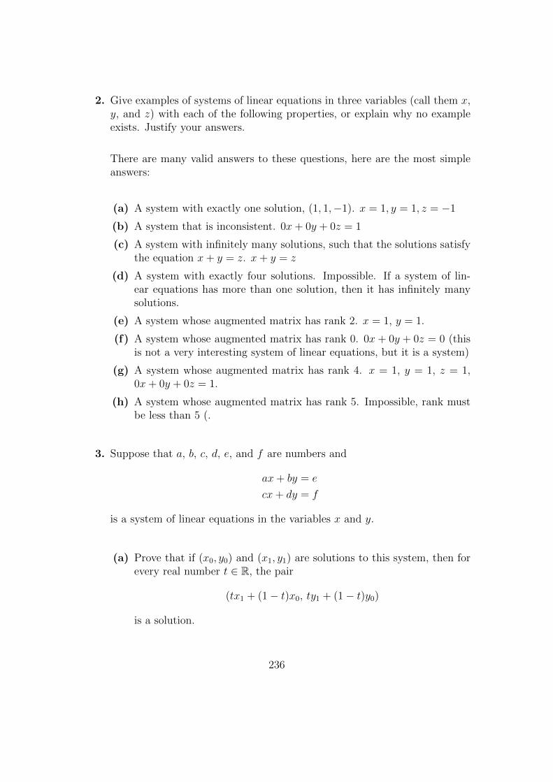
2. Give examples of systems of linear equations in three variables (call them x,y, and z) with each of the following properties, or explain why no exampleexists. Justify your answers.
There are many valid answers to these questions, here are the most simpleanswers:
(a) A system with exactly one solution, (1, 1,−1). x = 1, y = 1, z = −1
(b) A system that is inconsistent. 0x+ 0y + 0z = 1
(c) A system with infinitely many solutions, such that the solutions satisfythe equation x+ y = z. x+ y = z
(d) A system with exactly four solutions. Impossible. If a system of lin-ear equations has more than one solution, then it has infinitely manysolutions.
(e) A system whose augmented matrix has rank 2. x = 1, y = 1.
(f) A system whose augmented matrix has rank 0. 0x + 0y + 0z = 0 (thisis not a very interesting system of linear equations, but it is a system)
(g) A system whose augmented matrix has rank 4. x = 1, y = 1, z = 1,0x+ 0y + 0z = 1.
(h) A system whose augmented matrix has rank 5. Impossible, rank mustbe less than 5 (.
3. Suppose that a, b, c, d, e, and f are numbers and
ax+ by = e
cx+ dy = f
is a system of linear equations in the variables x and y.
(a) Prove that if (x0, y0) and (x1, y1) are solutions to this system, then forevery real number t ∈ R, the pair
(tx1 + (1− t)x0, ty1 + (1− t)y0)
is a solution.
236

Proof. To show that for any t ∈ R,
(tx1 + (1− t)x0, ty1 + (1− t)y0)
is a solution to the system of equations, we must plug these pairs ofnumbers into both equations and show that the equation is true.
For the first equation,
a(tx1 + (1− t)x0) + b(ty1 + (1− t)y0) = t(ax1 + by1) + (1− t)(ax0 + by0)
= t(e) + (1− t)(e)= e
so the equation is true.
For the second equation,
c(tx1 + (1− t)x0) + d(ty1 + (1− t)y0) = t(cx1 + dy1) + (1− t)(cx0 + dy0)
= t(f) + (1− t)(f)
= f
so the equation is true.
Since the pair satisfies both equations in the system, it is a solution ofthe system.
(b) Use part (a) to explain why a 2× 2 system of linear equations can onlyhave 0 solutions, 1 solution or infinitely many solutions.
Proof. First, without explaining anything, we know that there are threepossibilities: the system has 0 solutions, the system has 1 solution, orthe system has more than one solution.
We just need to explain why in the last case, if a system has more thanone solution, then it has infinitely many solutions.
If the system has more than one solution, then it has at least twosolutions. Let’s call those solutions (x0, y0), (x1, y1). Part (a) tells usthat if these two pairs are solutions, then every pair
(tx1 + (1− t)x0, ty1 + (1− t)y0)
237
is a solution as well. But since there are infinitely many numbers t ∈ R,this means there are infinitely many pairs
(tx1 + (1− t)x0, ty1 + (1− t)y0) .
So the system has infinitely many solutions.
4. If we multiply an equation by 0, then we can potentially introduce newsolutions to the system. For example, consider the system
x+ y = 2
x− y = 0.
It has a unique solution, (1, 1).
If we multiply the second equation in this system by 0, the system becomesjust x+ y = 2, whose solutions are of the form (1 + t, 1− t).
Thus, multiplying an equation by 0 can change the set of solutions to thesystem.
The point of elementary operations is that they don’t change the set of solu-tions. This is why the second elementary operation is multiplying an equa-tion by a nonzero number.
5. The following two statements are equivalent:
• The augmented matrix [A|b], corresponds to an inconsistent system oflinear equations.
• A row echelon form of [A|b] contains the row [0 · · · 0 1].
If a A row echelon form of [A|b] contains the row [0 · · · 0 1], then there is aleading entry in the last column of the row echelon form.
Since the row echelon form of [A|b] has r leading entries (rank = r), and oneof those leading entries is in the last column, A has r − 1 leading entries.
If the system is consistent, then all the leading 1’s in a row echelon form of[A|b] are in the coefficient part of the augmented matrix (not the last col-umn), so rank(A) = r = rank([A|b]).
238
For example, the augmented matrix in REF
[A|b] =
1 0 0 −1 1
252
0 1 0 −1 0 40 0 0 0 0 10 0 0 0 0 0
corresponds to an inconsistent system of equations because the third row is[0 0 0 0 0 1].
The rank of [A|b] is 3. The coefficient matrix
A =
1 0 0 −1 1
2
0 1 0 −1 00 0 0 0 00 0 0 0 0
has rank 3− 1 = 2.
Tutorial 2
1. (a) and (c) are equal. (b) and (d) are equal. In general, (e) and (f) are notequal (they don’t even have the same number of rows and columns! Onematrix is m×m, the other is n× n).
2. First, let
B =
[w xy z
]where w, x, y, z are variables we want to solve for.
Next, evaluate both sides of the matrix equation AB = BA,[1 11 0
] [w xy z
]=
[w xy z
] [1 11 0
][w + y x+ zw x
]=
[w + x wy + z y
].
239

This matrix equation is equivalent to the system of equations
w + y = w + x
x+ z = w
w = y + z
x = y
After a little work, we can solve this system and find that the solutions are
w = s+ t
x = s
y = s
z = t
for any s, t ∈ R. Thus the set of matrices B that solve the matrix equationis {[
s+ t ss t
]: s, t ∈ R
}
3. Consider the following list of algebraic identities and facts that are true whenx, y, and z are real numbers.
(a) A + B = B + A. By properties of matrix addition, this is always truewhen A,B are m× n matrices.
(b) AB = BA. This is not always true! For instance, take
A =
[1 00 −1
], B =
[0 11 0
](c) If AB = AC and A 6= 0, then B = C. This is not always true! For
instance, take
A =
[0 10 0
], B =
[1 00 0
], C =
[0 10 0
].
We see that A 6= 0 and B 6= C, but AB = AC.
4. (a) Can you find some or all solutions to the matrix equation X2 − I = 0?
There are a couple quick solutions, namely X = I and X = −I. Forthe others,
240

Write X as
X =
[a bc d
].
Then we have that
X2 =
[a2 + bc b(a+ d)c(a+ d) d2 + bc
].
For this to be equal to I, we need the following equations to all besatisfied:
a2 + bc = 1 (C.1)
b(a+ d) = 0 (C.2)
c(a+ d) = 0 (C.3)
d2 + bc = 1 (C.4)
(C.5)
We will solve this case by case. Since both b(a+d) = 0 and c(a+d) = 0,either both of b and c must be 0, or a+ d = 0. If b and c are 0, then weget that a2 = d2 = 1, which give the solutions:
[±1 00 ±1
].
If a + d = 0, then we have that a = −d. Then for any choice of a, b, cthat satisfy bc = 1− a2, the matrix
X =
[a bc −a
]will square to I.
(b) Is it possible to use Guassian elimination to solve this system of equa-tions? No. The system of equations (C.1) above is not a system oflinear equations in the variables (a, b, c, d).
6. A matrix A is called purple1 if A = AT . For each of the following statements,say whether it is true or false. Justify your answers with an explanation.
1The real word for this property is symmetric.
241

(i) False.
(ii) True.
(iii) False.
(iv) True.
(v) True.Proof: If A and B are purple, then
(A+B)T = AT +BT By properties of transpose.
= A+B Since A, B are purple.
so A+B is purple.
(vi) True.
(vii) True.Proof: We show BBT is purple. For any matrix B,
(BBT )T = (BT )TBT By properties of transpose.
= BBT By properties of transpose.
so BBT is purple.
(viii) True.
(ix) True.
(x) False.
Explanation: In general, properties of matrix algebra tell us that
(AB)T = BTAT By properties of transpose.
= BA Since A and B are purple.
but it is not always true that AB = BA! So it is not always true thatAB is purple.
(xi) True.
Proof: If A and B are purple, then
(ABA)T = ATBTAT By properties of transpose.
= ABA Since A, B are purple.
so ABA is purple.
242

(xii) True.
Tutorial 3
1. This system has augmented matrix: 3 2 −1 0 1 00 1 0 −1 0 0−1 −1 1 −3 0 0
It has RREF: 1 0 0 −1 1
20
0 1 0 −1 0 00 0 1 −5 1
20
Therefore, the set of solutions is{(
s− 1
2t, s, 5s− 1
2t, s, t
)|s, t ∈ R
}.
The solutions to the system in question 1, tutorial 1 will be given by anyparticular solution to that system plus a solution to this system.
An example of a particular solution to the non-homogeneous system of equa-tions from question 1, tutorial 1 is(
5
2, 4,
23
2, 0, 0
).
2. (i) True.
Explanation: 0−111
= (−1)
1100
+
1011
.so it is a linear combination of basic solutions, so it is a solution.
243
(ii) True.
Explanation: 6333
= 3
1100
+ 3
1011
.so it is a linear combination of basic solutions, so it is a solution.
(iii) False.
Explanation: The matrix equation0−111
= s
1100
+ t
1011
.has no solutions.
(iv) False.
Explanation: Looking at the form of the two basic solutions we aregiven, we can deduce that x1, x3 are leading variables and x2, x4 arefree variables.
Thus there are exactly two basic solutions (one for each free variable).
(v) True.
(vi) True.
Explanation: The rank of A equals the number of leading variables,which is 2.
(vii) True.
Explanation: We know from our explanation in part (d) that there areonly two basic solutions: u,v.
We know that the set of solutions to a homogeneous system equals thespan of the basic solutions.
244

3. Proof. Suppose that u1, . . .uk are solutions of the matrix equation Ax = b.If t1, . . . , tk are real numbers such that
t1 + t2 + · · ·+ tk = 1.
To show thatt1u1 + t2u2 + · · ·+ tkuk
is a solution of the matrix equation Ax = b we just need to plug it into theleft hand side of the equation and show that the equation is true.
A(t1u1 + t2u2 + · · ·+ tkuk) = A(t1u1) + A(t2u2) + · · ·+ A(tkuk) matrix algebra
= t1(Au1) + t2(Au2) + · · ·+ tk(Auk) matrix algebra
= t1(b) + t2(b) + · · ·+ tk(b) since Aui = b
= (t1 + t2 + · · · tk)b matrix algebra
= 1b since t1 + t2 + · · ·+ tk = 1
= b.
Thus, we have shown that
t1u1 + t2u2 + · · ·+ tkuk
is a solution of the matrix equation Ax = b.
4. If a system Ax = b has the trivial solution, then it is homogeneous. Explainwhy this is true.
The system has the trivial solution means that x = 0 is a solution.
This means that the equation A0 = b is true.
But 0 = A0 = b, so it must be the case that b = 0.
Since b = 0, the original equation Ax = b is homogeneous.
5. Suppose u and v are m×1 column vectors. Which of the following statementsare always true? Justify your answers.
245

(i) True. 0 = 0u + 0v, so u is a linear combination of u and v.
(ii) True. u = 1u + 0v.
(iii) True. 2u− v is a linear combination of u and v.
(iv) True. 2u−v = 1(2u−v) + 0(u + v). So 2u−v is a linear combinationof 2u− v and u + v.
(v) False. This is not always true. For example, u = [1 0]T , v = [1 1]T .
(vi) False. This is not always true. For example, u = [1 0]T , v = [2 0]T .Then b = [0 1]T is not in the span.
Suppose A is a m× 2 matrix with columns u and v as above. Which of thefollowing statements are always true? Justify your answers.
(i) True.
(ii) True.
(iii) True.
(iv) True.
(v) False. Compare with (f) above.
(vi) False.
Tutorial 4
1. A is invertible, B is not invertible.
2. By the big theorem for square matrices, the system has exactly one solutionif and only if A is invertible.
We know that the matrix [a bc d
]is invertible if and only if ad− bc 6= 0.
Thus, the system has exactly one solution if and only if ad− bc 6= 0.
246

3. Definition: A square matrix A is called orange2 if
ATA = I and AAT = I.
(i) The only elementary matrices that are orange are: the identity matrix,the elementary matrix corresponding to multiplying a row by -1, andthe elementary matrices corresponding to interchanging two rows.
(ii) Find two examples of orange matrices that aren’t elementary matrices(hint: try products of elementary matrices).
(iii) First, IT = I. Second, IT I = II = I and IIT = II = I.
(iv) A orange matrix is always invertible. What is the inverse? AT .
(v) Explanation: By definition, AT is invertible if there is a matrix B suchthat ATB = I and BAT = I.
We already know that ATA = I and AAT = I, so we know that AT isinvertible.
(vi) Proof: Suppose that A and B are orange matrices. We need to showthat (AB)(AB)T = I and (AB)T (AB) = I.
First,
(AB)(AB)T = (AB)(BTAT ) By properties of transpose.
= A(BBT )AT Matrix algebra.
= A(I)AT B is orange.
= (AI)AT Matrix algebra.
= AAT Matrix algebra.
= I A is orange.
2The real word for this property is orthogonal.
247

Second,
(AB)T (AB) = (BTAT )(AB) By properties of transpose.
= BT (ATA)B Matrix algebra.
= BT (I)B A is orange.
= BT (IB) Matrix algebra.
= BTB Matrix algebra.
= I B is orange.
4. Note first that the criteria that Ax = b has a solution for all b ∈ Rn isequivalent to A being invertible by the big theorem on square matrices (part1).
(i) True. (by big theorem)
(ii) True. (always true)
(iii) True. (as the b that make the system consistent are precisely the ele-ments of the span of the columns).
(iv) True. (by big theorem and in particular the matrix inversion algorithm)
(v) True. (the transpose of an invertible matrix is invertible)
(vi) True. (similar to (c) )
(vii) True. (by big theorem and the fact that A−1 is invertible).
(viii) True. (by big theorem)
(ix) True. (since A is invertible, A3 is invertible).
5. Use the Big Theorem for Square Matrices to prove the following statement.
If A is invertible, then A does not have a row of zeros.
Proof. By the big theorem, since A is invertible, we know that the rank ofA is n.
Since the rank of A is n, any REF of A has n leading entries.
Since A is n × n, this means that every row in the REF of A contains aleading entry.
248

Thus, A cannot have a row of zeros (since there would be a row of zeros inthe REF).
If A does not have a row of zeros, then A is invertible.
This statement is false. For example, the matrix[1 11 1
]does not have a row of zeros, and it is not invertible.
C.2 Tutorial 5-8
Tutorial 5: Vector geometry
Background: Chapter 5 of the lecture notes.
1. (i) Find the equation of the plane that contains the points
(2, 4, 4), (2,−2, 2), (4, 2, 2) ∈ R3.
Solution: We will give these points names: P0 = (2, 4, 4), P1 = (2,−2, 2),and P2 = (4, 2, 2).
We calculate that−−→P0P1 =
0−6−2
, and−−→P1P2 =
240
.
Let a =−−→P0P1 ×
−−→P1P2 =
8−412
.
Therefore, the equation of the plane containing P0, P1, and P2 is a·x = b,and we just need to calculate b. To do this we plug in one point. P1 willgive us: b = (8)(2) + (−4)(−2) + (12)(2) = 48. Therefore the equationof the plane is
8x− 4y + 12z = 48.
249
(ii) Find the equation of the plane that contains the points
Q0 = (2, 1, 3), Q1 = (3, 0, 2), Q2 = (3, 3, 3) ∈ R3.
Solution: First,
−−−→Q0Q1 =
1−1−1
, −−−→Q0Q2 =
120
.Second,
a =−−−→Q0Q1 ×
−−−→Q0Q2 =
2−13
.The equation of the plane is then
a · x = a ·Q0
which gives2x1 − x2 + 3x3 = 12.
(iii) Show that the two planes from part (a) and part (b) are the same.
Solution: The equation we obtained in part (a) was
8x− 4y + 12z = 48.
The equation we obtained in part (b) was
2x1 − x2 + 3x3 = 12.
The first equation equals 4 times the second equation, so the set ofsolutions to these two equations is the same. (in other words, these twosystems of one equation differ by a single elementary operation).
2. (i) Show that the three points
P0 = (5, 6, 1), P1 = (−1,−2, 3), P2 = (11, 14,−1)
are collinear.
Solution: We can see by inspection that
P2 = 2P0 − P1 = (1− (−1))P0 + (−1)P1,
so the three points are collinear.
250

(ii) Describe all the planes that contain all three points, P0, P1, P2 (thereare infinitely many).
Solution: The line containing the three points is parallel to the vector
d =−−→P0P1 = (−6,−8, 2).
The set of vectors that are orthogonal to d (normal vectors to planesthat contain the line) is the set
{n = (n1, n2, n3) ∈ R3 : n · d = 0}
Which is just the set of solutions of the equation
−6n1 − 8n2 + 2n3 = 0.
After solving this system we find
{n = (n1, n2, n3) ∈ R3 : n·d = 0} = {n = ((t−4s)/3, s, t) ∈ R3 : s, t ∈ R}.
All the planes containing the line are of the form
n · x = n · P0
t− 4s
3x1 + sx2 + tx3 =
5(t− 4s)
3+ 6s+ t.
where for each plane the numbers s, t ∈ R have been fixed, and x1, x2, x3are the variables.
Notice that some of these equations will determine the same plane, butthere is still infinitely many planes that contain this line.
3. (i) Show that if two vectors u,v ∈ Rn are parallel, then
projuv = v.
Solution: If u and v are parallel, that means that ku = v for somescalar k. Therefore
proju(v) =u · vu · u
u by definition of proj
= ku · uu · u
u since ku = v
= ku cancelling
= v since ku = v
251

(ii) Show that if u,v ∈ Rn are orthogonal, then
projuv = 0.
Solution: If u and v are orthogonal then u · v = 0, so
proju(v) =u · vu · u
u =0
u · uu = 0u = 0.
(iii) Show that for any vectors u,v ∈ Rn,
||projuv|| ≤ ||v||.
Solution 1: We use the Cauchy-Schwartz inequality in the key step.
||proju(v)|| = ||u · vu · u
u|| definition of proj
= |u · vu · u
|||u|| sinceu · vu · u
is a scalar.
=|u · v||u · u|
||u||
=|u · v|||u||2
||u||
=|u · v|||u||
≤ ||u||||v||||u||
Cauchy-schwartz
= ||v||
Solution 2: ||proju(v)||2 = (u·vu·uu) · (u·v
u·uu) = (u·v)2u·u = ||u||2||v||2 cos2 θ
||u||2 =
||v||2 cos2 θ ≤ ||v||2
4. Show that for any two vectors, u = [u1 u2 u3] and v = [v1 v2 v3], the vector
x = u× v
is a solution of the matrix equation[u1 u2 u3v1 v2 v3
]x = 0.
252
Solution: Note that by definition of matrix-vector multiplication,[u1 u2 u3v1 v2 v3
]x =
[u · xv · x
].
By properties of the cross-product, we know that (u × v) · u = 0 and (u ×v) · v = 0. Thus[
u1 u2 u3v1 v2 v3
](u× v) =
[u · (u× v)v · (u× v)
]=
[00
]so u× v is a solution.
5. Three points, P0, P1, P2 ∈ R3 are called collinear if they all lie on the sameline.
(i) Are the points (0, 0, 0), (1, 0, 0), (−10, 0, 0) collinear? Solution: Yes
(ii) Are the points (0,−1, 4), (0,−1, 7), (0,−1, 10) collinear? Solution: Yes
(iii) Are the points (2, 0, 0), (0, 1, 0), (0, 0, 1) collinear? Solution: No
(iv) Show that the following two statements are equivalent:
• P0 = (x0, y0, z0), P1 = (x1, y1, z1), P2 = (x2, y2, z2) are collinear.
• There is a number t ∈ R such that
x2 = tx1 + (1− t)x0y2 = ty1 + (1− t)y0z2 = tz1 + (1− t)z0
Solution: P0, P1, P2 collinear means that P2 lies on the line determinedby P0 and P1. This means that P2 is contained in the line
L ={P0 + t
−−→P0P1 : t ∈ R
}.
P2 ∈ L means there is a number t ∈ R so that (using vector notation)
P2 = P0 + t−−→P0P1 =
x0y0z0
+ t
x1 − x0y1 − y0z1 − z0
=
tx1 + (1− t)x0ty1 + (1− t)y0tz1 + (1− t)z0
.253

(v) Use part (d) to show that if P0, P1, P2 are collinear, then the matrix x0 y0 z0x1 y1 z1x2 y2 z2
has rank ≤ 2.
Solution: By part (d), we know that if P0, P1, P2 are collinear, thenthere is a number t ∈ R so that
x2 = tx1 + (1− t)x0y2 = ty1 + (1− t)y0z2 = tz1 + (1− t)z0
Thus x0 y0 z0x1 y1 z1x2 y2 z2
=
x0 y0 z0x1 y1 z1
tx1 + (1− t)x0 ty1 + (1− t)y0 tz1 + (1− t)z0
Thus if we perform the row operations “subtract t times R2 to R3” and“subtract 1− t times R1 to R3”, then the result will be x0 y0 z0
x1 y1 z10 0 0
so the matrix must have rank ≤ 2.
This fact can be useful for checking whether three points are collinear,since it is often easy to compute the rank of a matrix.
6. Consider the two vectors
u =
12−1
,v =
011
(i) Show that u and v are not parallel.
254

Solution: If k
12−1
=
011
, we have that simultaneously k must be
0 and 1/2, so there can be no such k. Therefore these vectors are notparallel.
(ii) Write the equation of the plane through the origin determined by thevectors u and v (use the cross-product to find a normal vector).
Solution: u × v =
2 · 1− (−1) · 1(−1) · 0− 1 · 1
1 · 1− 2 · 0
=
3−11
. Therefore the plane
going through the origin determined by these two vectors is
(u× v) ·
xyz
=
3−11
·xyz
= 3x− y + z = 0.
(iii) Show that the plane through the origin determined by the vectors uand v equals the set
span{u,v}.
This has two steps:
• Show that any linear combination tu+sv is a solution to the equa-tion from part (b).
• Show that any point that solves the equation from part (b) can bewritten as a linear combination tu + sv.
Solution: Let’s use the notation
P ={
(x, y, z) ∈ R3 : 3x− y + z = 0}.
• Any linear combination tu + sv is a solution to the equation frompart (b), since
(u× v) · (tu + sv) = s(u× v) · u + t(u× v) · v = s0 + t0 = 0.
Thus we know that span{u,v} ⊆ P . (note that this argumentworks for any plane through the origin since we just used proper-ties of dot and cross products).
255

7. Let Q1 = (1,−1) and Q2 = (−1, 1). Describe the set of points P = (x, y)such that
d(P,Q1) = d(P,Q2).
Solution: For P = (x, y), we have
d(P,Q1) =√
(x− 1)2 + (y + 1)2
d(P,Q2) =√
(x+ 1)2 + (y − 1)2
Thus the conditiond(P,Q1) = d(P,Q2)
simplifies to(x− 1)2 + (y + 1)2 = (x+ 1)2 + (y − 1)2
Expanding both sides gives
x2 − 2x+ 1 + y2 + 2y + 1 = x2 + 2x+ 1 + y2 − 2y + 1
and this simplifies tox = y.
Thus the set of all points is the line
L = {(x, y) ∈ R2 : x = y}.
256

8. (bonus) The area of a parallelogram in R2 with adjacent sides u and v canbe computed with the formula
Area = ||u||||v|| sin(θ)
where θ is the angle between u and v.
Use this formula and other properties of angles and dot products to show
that if u =
[ac
]and v =
[bd
], then
Area = ad− bc.
Solution: We know that the area of the triangle satisfies
Area2 = ||u||2||v||2 sin2(θ) = ||u||2||v||2(1− cos2(θ)) = ||u||2||v||2 − (u · v)2.
Plugging in u =
[ac
]and v =
[bd
], we get
Area2 = ||u||2||v||2 − (u · v)2
= (a2 + c2)(b2 + d2)− (ab+ cd)2
= a2b2 + a2d2 + c2b2 + c2d2 − a2b2 − 2abcd− c2d2
= a2d2 − 2abcd+ b2c2
= (ad− bc)2
ThusArea = ad− bc.
Tutorial 6: Linear transformations
Background: Chapter 6 of the lecture notes.
1. Suppose that
u =
121
, v =
101
, w =
110
.Let T be the linear transformation such that
T (u) =
100
, T (v) =
010
, T (w) =
001
.257

(i) Use properties of linear transformations to find the matrix of T .
Solution: First, after some thought, we see that
e1 = w − 1
2u +
1
2v
e2 =1
2u− 1
2v
e3 =1
2v −w +
1
2u
By properties of linear transformations, we know that
T (e1) = T (w − 1
2u +
1
2v)
= T (w)− 1
2T (u) +
1
2T (v)
=
−1/21/21
T (e2) = T (
1
2u− 1
2v)
=1
2T (u)− 1
2T (v)
=
1/2−1/2
0
T (e3) = T (
1
2v −w +
1
2u)
=1
2T (v)− T (w) +
1
2T (u)
=
1/21/2−1
Thus, the matrix of T is −1/2 1/2 1/2
1/2 −1/2 1/21 0 −1
(ii) This linear transformation is invertible. Use the matrix from part (a)
to compute the matrix of T−1.
258

Solution: Using matrix inversion algorithm to compute the inverse ofthe matrix from part (a).
(iii) There is another (quicker) way to find the matrix of T−1 without usingthe matrix from part (a). What is it?
Solution: The inverse linear transformation T−1 satisfies T−1(T (x)) =x. Thus from what we are given, we know that
T−1(e1) = u, T−1(e2) = v, T−1(e3) = w.
Thus the matrix of T−1 is
[u|v|w] =
1 1 12 0 11 1 0
.
3. For each item below, give an example of a linear transformation with thatproperty or explain why no linear transformation with that property exists.
(i) T is injective and surjective.
Solution: T (x, y) = (x, y) is both injective and surjective.
(ii) T is injective but not surjective.
Solution: T : R2 → R3 given by T (x, y) = (x, y, 0) is injective but notsurjective.
(iii) T is surjective but not injective.
Solution: T : R3 → R2 given by T (x, y, z) = (x, y) is surjective but notinjective.
(iv) T : R3 → R3 is invertible.
Solution: T : R3 → R3 given by T (x, y, z) = (x, y, z) is invertible.
259

(v) T : R3 → R3 is invertible but not injective.
Solution: This is impossible by Theorem in the lecture notes.
(vi) T : R3 → R3 is injective but not surjective.
Solution: This is impossible. By Theorem , since T is injective, it isinvertible. By Theorem , since T is invertible, it is surjective.
(vii) For every nonzero vector x, T (x) 6= x and T ◦ T (x) = x.
Solution: T : R2 → R2 given by T (x, y) = (−x,−y).
(viii) T : R3 → R3 and the image of T is span{[1 5 2]T}.
Solution: T : R3 → R3 given by orthogonal projection onto the linespanned by [1 5 2]T .
(ix) T : R→ R3 and the image of T is span{[1 5 2]T}.
Solution: Take TA where
A =
152
.Solution:
(x) T : R2 → R3 and the image of T is span{[1 5 2]T}.
Solution: Take TA where
A =
1 15 52 2
.
4. Given a column vector u =
u1...un
∈ Rn.
We know that uTu is a number, and uuT is a n× n matrix.
260
(i) Use the definition of the orthogonal projection projux to show thatthe matrix of the linear transformation T (x) = projux is given by theformula
A =1
uTuuuT .
Solution: We simply need to check that for all x,
projux =1
uTuuuTx.
This is true since
projux =u · xu · u
u by definition of orthogonal projection
= u
(uTx
uTu
)properties of dot-product
=u(uTx)
uTurearranging
=(uuT )x
uTuassociativity of matrix mult.
=1
uTuuuTx rearranging again.
(ii) Use the result from part (a) to compute the matrix of the orthogonal
projection proju : R3 → R3 for the vector u =
−121
.
Solution: The matrix
A =1
uTuuuT =
1
6
1 −2 −1−2 4 2−1 2 1
.(iii) For the orthogonal projection in part (b), write the sets ker(proju) and
im(proju) as the span of a set of vectors.
Solution:
• The image of orthogonal projection onto a line is the line itself, so
image(T ) = span
−1
21
.
261

• The kernel of orthogonal projection on to the line equals the setof solutions to the equation Ax = 0. We can find a spanning setfor this set by computing the basic solutions of this homogeneoussystem, which gives
ker(T ) = span
2
10
, 1
01
.
Another way to understand this solution is that we have found aspanning set for the plane through O with normal vector u.
(iv) Use the result from part (a), and properties of matrix algebra, to showthat the matrix A of orthogonal projection onto a line is always purple(Remember, A is purple if A = AT ).
Solution: Using properties of matrix algebra, we check that
AT =
(1
uTuuuT
)T=
1
uTu
(uuT
)Tsince
1
uTuis a scalar
=1
uTu(uT )TuT properties of matrix transpose
=1
uTuuuT properties of matrix transpose
= A.
5. A linear transformation T : Rn → Rn is called covfefe if for every vectorx ∈ Rn,
||T (x)|| = ||x||.
(i) Which of the following linear transformations R2 → R2 are covfefe?
i. Rotation by θ degrees is covfefe.
ii. Reflection through a coordinate axis is covfefe.
iii. Scaling (dilation) by a factor of k is only covfefe if k = ±1.
iv. The shear transformation with matrix[1 a0 1
]is only covfefe if a = 0.
262

v. Orthogonal projection onto a line through the origin is never cov-fefe.
(ii) Describe in words what a covfefe transformation does geometrically.
Solution: A covfefe transformation preserves the lengths of vectors (al-terantively, one could say that a covfefe transformation preserves thedistance of points from the origin).
(iii) Recall that a square matrix A is called orange if AAT = ATA = I.Show that if A is orange, then the linear transformation TA(x) = Ax iscovfefe.
Solution: If A is orange, then we check
||TA(x)||2 = ||Ax||2 by definition of TA
= (Ax) · (Ax) properties of vector length
= (Ax)T (Ax) properties of dot product
= xTATAx properties of matrix transpose
= xTx since A is orange
= ||x||2
Thus ||TA(x)|| = ||x||.(iv) Show that if a linear transformation T is covfefe, then ker(T ) = {0}.
Solution: In order to show equality of two sets, we must show thatker(T ) ⊆ {0} and {0} ⊆ ker(T ). The second inclusion is true for anylinear transformation, so we only need to check the first one.
To see that ker(T ) ⊆ {0}, we use the definition of ker(T ).
If x ∈ ker(T ), then T (x) = 0.
Since T is covfefe, this implies that
||x|| = ||T (x)|| = ||0|| = 0.
But if ||x|| = 0, then x = 0.
263

(v) Use the result of part (d) and the Theorems from section 6.9 of thelecture notes to explain why every covfefe linear transformation is in-vertible.
Solution: By part (d), we know that T is injective. By Theorem 6.23,this tells us that T is invertible.
(vi) Use the result of part (e) and the Theorems from section 6.9 of thelecture notes to explain why every covfefe linear transformation is sur-jective.
Solution: By part (e) we know that T is invertible. By Theorem 6.24in the lecture notes, this tells us that T is surjective.
Tutorial 7:
Background: Chapter 7 of the lecture notes.
1. Let
E =
0 0 10 1 01 0 0
.and
u =
20−1
, v =
121
, w =
100
.(i) Compare the subspaces S = span{u} and S ′ = span{Eu}. Solution:
They are different.
(ii) Compare the subspaces S = span{v} and S ′ = span{Ev}. Solution:They are the same.
(iii) Compare the subspaces S = span{u,v} and S ′ = span{Eu, Ev}.
Solution: They are different. Indeed,
S = span{u,v} = span
2
0−1
, 1
21
264

and
S ′ = span{Eu, Ev} = span
−1
02
, 1
21
.
The vector
−102
∈ S ′, but it is not contained in S since
−102
= s
20−1
+ t
121
=
2s+ t2tt− s
has no solutions. (first, t must be 0, but then the third and first entriesare the equations −1 = 2s and 2 = −s, which has no solutions).
Since S ′ contains a vector that is not in S, the two sets are different.
(iv) Compare the subspaces S = span{u,w} and S ′ = span{Eu, Ew}.
Solution: They are the same. Indeed,
S = span{u,w} = span
2
0−1
, 1
00
S ′ = span{Eu, Ew} = span
−1
02
, 0
01
.
If you look carefully at both of these spans, you will see that both ofthem equal the subspace
x0z
∈ R3 : x, z ∈ R
In other words, the sets {u,w} and {Eu, Ew} are two different basesfor the same subspace.
One way to describe what is happening here is that the transformationgiven by E, TE : R3 → R3 preserves the subspace above, since for any
265

vector in this subspace,
TE
x0z
= E
x0z
=
z0x
which is still in the subspace.
(v) Compare the subspaces S = span{u,v,w} and S ′ = span{Eu, Ev, Ew}.Solution: They are the same. They are both 3 dimensional spaces inR3, so they both must be R3.
2. Which of the following sets are subspaces of R2? Justify your answer. Drawa picture of what the set looks like.
(i) A line is not a subspace unless it contains the origin.
(ii) A point is not a subspace unless it is the origin.
(iii) A circle of radius 2 centred at (0, 2) is not a subspace.
(iv) R2 is a subspace.
(v) The set of points equidistant from (1, 1) and (−1,−1) is a subspace (itis the line y = −x).
(vi) The set of points {(x, y) ∈ R2 : y = x2} is not a subspace (it failsconditions II) and III).
(vii) The set of points {(x, y) ∈ R2 : x ≥ 0} is not a subspace. It failscondition III).
(viii) The set of points {(x, y) ∈ R2 : x2 ≥ 0} equals R2, which is a subspace.
3. True or false.
(i) If S is a subspace of Rn, then dim(S) < n. Solution: False. S could beRn in which case dim(S) = n. Otherwise dim(S) < n.
(ii) If S is a subspace of Rn, then dim(S) > 0. Solution: False. S could bethe zero subspace, {0}, in which case dim(S) = 0. Otherwise dim(S) >0.
(iii) If {u,v} is a set of two vectors in R3, then there is a vector w so that{u,v,w} is a basis for R3. Solution: False. It is only true if {u,v} islinearly independent.
266

(iv) If {u,v,w,x} is a set of vectors in R3, then it is linearly dependent.Solution: True. The maximum size of a linearly independent subset ofR3 is 3.
(v) If 0 is not contained in a set of vectors U , then U is linearly independent.
Solution: False. For example {[10
],
[−10
]} is linearly dependent.
(vi) If S and S ′ are subspaces of Rn with dim(S) = dim(S ′), then S = S ′.Solution: . False. For example, any two lines through the origin in R2
have dimension 1.
4. Suppose S is a set of points in Rn and T : Rn → Rm is a linear transformation.
Define the setS ′ = {T (x) : x ∈ S} ⊆ Rm.
We call S ′ the image of S under T .
(i) Let S be the line through the origin in R2 spanned by u =
[21
].
i. If T is the linear transformation “rotate by an angle of π/2 radiansclockwise” then what is the image of S under T?
Solution: The image of S under T is the line span{[
1−2
]}.
ii. If TA is the linear transformation corresponding to the matrix
A =
[1 −2−2 4
].
then what is the image of S under T?
Solution: SinceA
[21
]= 0, so the image of S under TA is span{A
[12
]} =
{0}.
(ii) Show using the definition of subspace that if S is a subspace of Rn, thenthe image S ′ of S under a linear transformation T is a subspace of Rm.Solution: We check each condition of being a subspace.
267

I) Since S is a subspace, 0 ∈ S. Since T is a linear transformation,T (0) = 0. Thus 0 ∈ S ′.
II) If u,v ∈ S ′, then u = T (x) and v = T (y) for x,y ∈ S.
Since S is a subspace, x + y ∈ S, so T (x + y) ∈ S ′. Finally, sinceT is a linear transformation,
T (x + y) = T (x) + T (y) = u + v.
Thus u + v ∈ S ′.
III) Suppose u = T (x) ∈ S ′ and k ∈ R.
Since S is a subspace, kx ∈ S. Thus T (kx) ∈ S ′. Finally, since Tis a linear transformation,
T (kx) = kT (x).
Thus kT (x) ∈ S ′.Solution 2: We can use the subspace test.
If y,y′ are vectors in S ′, and k ∈ R, then there are vectors x,x′ in Sso that T (x) = y, and T (x′) = y′. Since S is a subspace, x + kx′ ∈ S,so therefore y + ky′ = T (x + kx′), so y + ky′ ∈ S ′, showing that S ′ isa subspace.
(iii) Show that if S = span{u1, . . . ,uk}, then S ′ = span{T (u1), . . . , T (uk)}.
Solution: Suppose that y ∈ S ′. Then y = T (x) for some x ∈ S.Since S = span{u1, . . . ,uk }, there are scalars t1, . . . , tk, so that x =t1u1 + . . . + tkuk. Therefore y = T (x) = T (t1u1 + . . . + tkuk) =t1T (u1) + . . .+ tkT (uk).
(iv) Show that if S is a subspace of Rn, then dim(S ′) ≤ dim(S).
Solution: If {u1, . . . ,uk } is a basis for S, then by the result of theprevious item, {T (u)1, . . . , T (uk) } contains a basis for S ′. Thereforedim(S) = k ≥ dim(S ′).
268
5. In this question we will finish a detail from the proof of the algorithm forfinding a basis of the span of a set of vectors.
Show that if
• {u1, . . . ,uk} is a set of linearly independent vectors in Rn, and
• A is an invertible n× n matrix,
then the set{Au1, . . . , Auk}
is linearly independent.
Solution: To show that {Au1, . . . , Auk} is linearly independent, we showthat the only solution to the equation
x1(Au1) + · · ·+ xk(Auk) = 0
is x1, . . . , xk = 0.
By matrix algebra,
x1(Au1) + · · ·+ xk(Auk) = A(x1u1 + · · ·+ xkuk).
Since A is invertible, if A(x1u1 + · · ·+xkuk) = 0, then x1u1 + · · ·+xkuk = 0.
Finally, since {Au1, . . . , Auk} is linearly independent, if x1u1+· · ·+xkuk = 0,then x1, . . . , xk = 0.
Tutorial 8
Background: Chapter 8 of the lecture notes.
1. Let
A =
1 −2 0 0 32 −5 −3 −2 60 5 15 10 02 6 18 8 6
269

The reduced row echelon form of A is
R =
1 −2 0 0 30 1 3 2 00 0 1 1 00 0 0 0 0
(i) What is the rank of A? 3
(ii) Find a basis for null(A). What is the nullity of A?
null(A) = 2
(iii) Find a basis for col(A). What is the dimension of the column space of A?
dim(col(A)) = 3
(iv) Find a basis for row(A). What is the dimension of the row space of A?
dim(row(A)) = 3
(v) Check the rank-nullity theorem for A.
2 + 3 = 5
(vi) Write a basis for the column and row space of AT .
(hint: the rows of A are the columns of AT and vis versa)
(vii) What is the rank of AT ? Why?
rank(AT ) = rank(A) = 3
(viii) What is the dimension of the null space of AT ?
dim(null(AT ) = 4− rank(AT ) = 4− 3 = 1.
270
2. In this question we will explore examples and theory related to Theorem 8.9in the lecture notes.
(i) Are the statements in Theorem 8.9 true for the matrix
A =
1 −22 −50 52 6
?
Solution: Yes
(ii) Are the statements in Theorem 8.9 true for the matrix
A =
[1 −2 12 −5 0
]?
Solution: No
(iii) Are the statements in Theorem 8.9 true for the matrix
A =
[1 72 −5
]?
Solution: Yes. But this matrix is also invertible so the statements inTheorem 8.8 are also true.
(iv) Is it possible for any of the statements in Theorem 8.9 to be true for amatrix with fewer columns than rows (m < n)? Why?
Solution: No. If m < n, then rank(A) ≤ m < n. Thus rank(A) = n isimpossible.
(v) Use the result from part (d) to explain the following fact.
Fact: If A is a m× n matrix and m < n, then the matrix equation
XA = In
has no solutions (i.e. there is no n×m matrix X that solves this equa-tion). In other words, A cannot have a left inverse.
Solution: By part (d), all of the equivalent statements in Theorem 8.9are false for A.
271
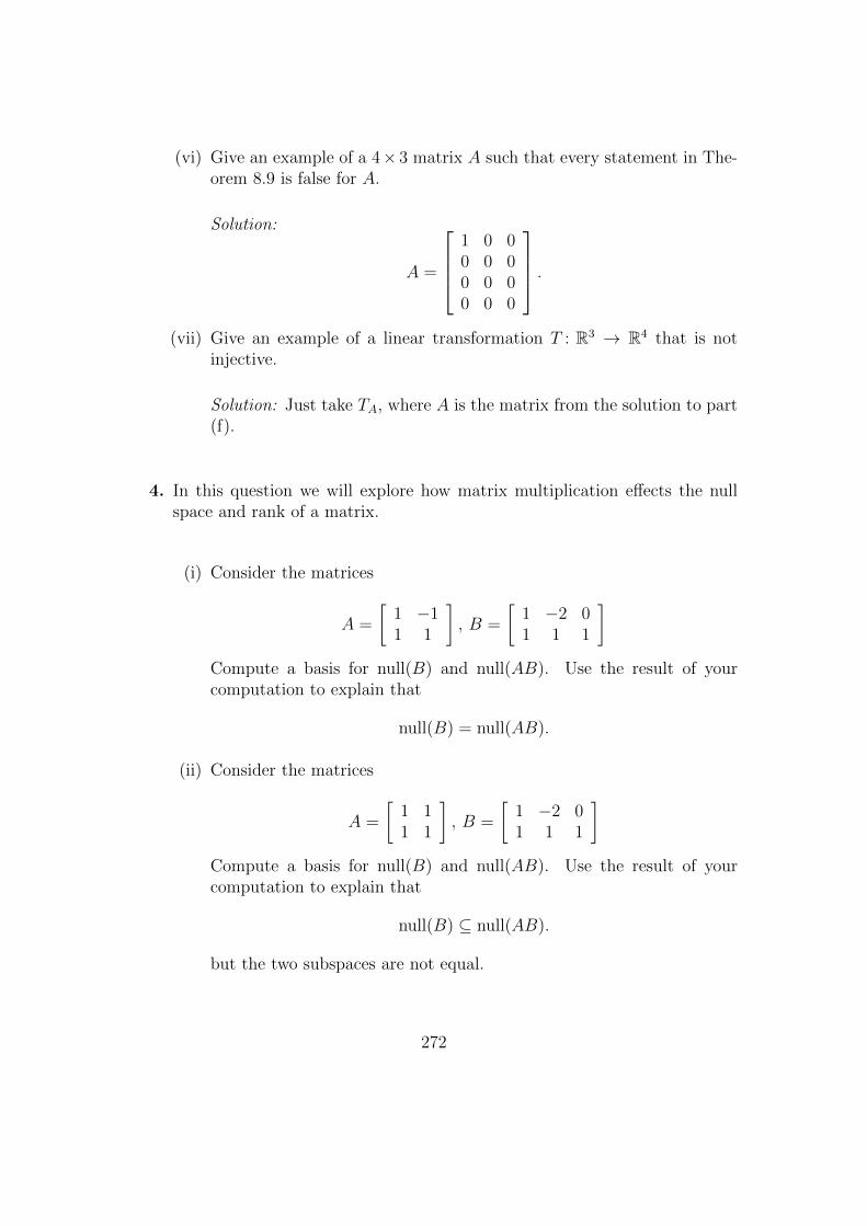
(vi) Give an example of a 4× 3 matrix A such that every statement in The-orem 8.9 is false for A.
Solution:
A =
1 0 00 0 00 0 00 0 0
.(vii) Give an example of a linear transformation T : R3 → R4 that is not
injective.
Solution: Just take TA, where A is the matrix from the solution to part(f).
4. In this question we will explore how matrix multiplication effects the nullspace and rank of a matrix.
(i) Consider the matrices
A =
[1 −11 1
], B =
[1 −2 01 1 1
]Compute a basis for null(B) and null(AB). Use the result of yourcomputation to explain that
null(B) = null(AB).
(ii) Consider the matrices
A =
[1 11 1
], B =
[1 −2 01 1 1
]Compute a basis for null(B) and null(AB). Use the result of yourcomputation to explain that
null(B) ⊆ null(AB).
but the two subspaces are not equal.
272

(iii) Show that, in general, if A is a m× n matrix and B is a n× p matrix,then
null(B) ⊆ null(AB).
Proof. Suppose that v ∈ null(B) (this means that Bv = 0).
Then ABv = A(Bv) = A0 = 0.
Therefore v ∈ null(AB).
Since we have shown that every element of null(B) is an element ofnull(AB), we have shown that
null(B) ⊆ null(AB).
(iv) (bonus) Use part (c) and the rank-nullity theorem to conclude the fol-lowing theorem:
Theorem: If A is a m× n matrix and B is a n× p matrix, then
rank(B) ≥ rank(AB).
Proof. The rank-nullity theorem for the m× p matrix AB tells us that
p = rank(AB) + nullity(AB).
The rank-nullity theorem for the n× p matrix B tells us that
p = rank(B) + nullity(B).
Combining these two equations gives us the equation
rank(AB) + nullity(AB) = rank(B) + nullity(B).
By part (c), we know that null(B) ⊆ null(AB), so nullity(B) ≤ nullity(AB).
Therefore since
rank(AB) + nullity(AB) = rank(B) + nullity(B)
and nullity(B) ≤ nullity(AB), we know that
rank(B) ≥ rank(AB).
273

(v) There is a similar but slightly different fact:
Theorem: If C is a n×m matrix and D is a p× n matrix, then
rank(D) ≥ rank(DC).
Solution:
Proof. We can use part (d) and the magic of matrix transposes. We seethat
rank(DC) = rank(CTDT ) since transpose does not change rank
≤ rank(DT ) by part (d)
= rank(D) since transpose does not change rank
(vi) In part (a), we saw an example where A was invertible and we observedthat null(B) = null(AB).
In fact, this is true in general:
Theorem: If A is an invertible n× n matrix and B is a n× p matrix,then
null(B) = null(AB).
Prove this theorem.
Proof 1: To show that the two sets are equal, we show two things.
First, by part (c), we already know that null(B) ⊆ null(AB).
Second, we can show that if A is invertible, then null(AB) ⊆ null(B).
Indeed, if A is invertible, and x ∈ null(AB), then
Bx = (A−1A)Bx = A−1(ABx) = A−1(0) = 0.
Thus, x ∈ null(B).
274

finally, since we have shown that null(B) ⊆ null(AB) and null(AB) ⊆null(B), we know that
null(B) = null(AB).
Proof 2: By part (c), we know that null(B) ⊆ null(AB).
Thus, in order to show that null(B) = null(AB), it is sufficient to ex-plain why they have the same dimension (since by Theorem 7.12(g), ifS ⊆ S ′ and dim(S) = dim(S ′), S = S ′).
Since A is invertible, we know that rank(AB) = rank(B) (this is truesince A is a product of elementary matrices). By the rank-nullity the-orem, this tells us that
dim(null(AB)) = n− rank(AB) = n− rank(B) = dim(null(B)).
This completes the proof.
C.3 Tutorial 9-11
Tutorial 9: Determinants
Background: Chapter 9 of the lecture notes.
1. (warm-up) Use cofactor expansion to compute the determinant of the fol-lowing matrices.
(i) det(A) = 3
(ii) det(B) = −28
(iii) det(C) = −84
(iv) In general, det
([A 0m×nD B
])= det(A) det(B).
2. Find the determinant of the following matrices by inspection (don’t use co-factor expansion, instead use properties of determinants and to quickly “see”the determinant without computing).
275

(i) det
4 0 0 0 00 −1 0 0 00 0 2 0 00 0 0 2 00 0 0 0 8
= 4(−1)(2)(2)(8).
(ii) det
4 3 43243 5 1213210 2 2 1000 100 0 2 82 93922340 0 0 3 650 0 0 0 −1
= (4)(2)(2)(3)(−1)
(iii) det
1 0 4 0 00 1 0 0 00 −2 1 0 00 0 0 6 00 0 0 0 1
= 6
(iv) det
0 1 0 0 01 0 0 0 00 0 0 1 00 0 1 0 00 0 0 0 1
= (−1)(−1)(1) = 1
(v) det
0 0 0 0 10 1 0 0 00 0 100 0 00 0 0 1 01 0 0 0 0
= (−1)(100) = −100
(vi) det
0 0 0 0 10 0 0 0 00 0 100 0 00 0 0 1 01 0 0 0 0
= (−1)(0)(100) = 0
3. Suppose that A and B are 3×3 matrices with det(A) = −1 and det(B) = 2.Compute each of the following determinants using properties of the determi-nant.
(i) det(2A2) = 23(−1)(−1)
(ii) det(A3B5) = (−1)3(2)5
(iii) det(BABABAB2) = (−1)3(2)5
276

(iv) det(3A2B−1) = 33(−1)2(1/2)
(v) det(3(A2B−1)T ) = det(3A2B−1) = 33(−1)2(1/2)
4. Consider the matrix
A =
[1 2 01 0 3
].
(i)det(AAT ) = 49
(ii)det(ATA) = 0
(iii) The problem with the fake proof is the step det(AAT ) = det(A) det(AT ).Since A is not a square matrix, the expressions det(A) and det(AT )aren’t defined, so this step is nonsense.
Tutorial 10: Eigenvalues, eignevectors, and diagonalization
Background: Chapter 10 of the lecture notes.
1. Compute the eigenvalues and corresponding eigenspaces for the matricesbelow. Which of the matrices are diagonalizable? For each matrix that isdiagonalizable, compute its diagonalization.
(i) [7 4−3 −1
]Eigenvalues: 1,5.
E1 = span
{[−23
]}E5 = span
{[−21
]}There are two distinct eigenvalues, so this matrix is diagonalizable. Onepossible diagonalization is[
7 4−3 −1
]=
[−2 −23 1
] [1 00 5
] [1/4 1/2−3/4 −1/2
]
277
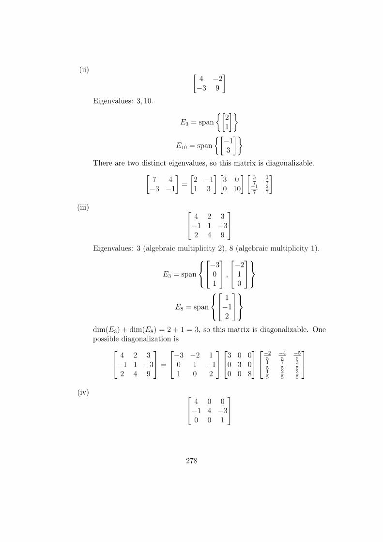
(ii) [4 −2−3 9
]Eigenvalues: 3, 10.
E3 = span
{[21
]}E10 = span
{[−13
]}There are two distinct eigenvalues, so this matrix is diagonalizable.[
7 4−3 −1
]=
[2 −11 3
] [3 00 10
] [37
17
−17
27
](iii) 4 2 3
−1 1 −32 4 9
Eigenvalues: 3 (algebraic multiplicity 2), 8 (algebraic multiplicity 1).
E3 = span
−3
01
,−2
10
E8 = span
1−12
dim(E3) + dim(E8) = 2 + 1 = 3, so this matrix is diagonalizable. Onepossible diagonalization is 4 2 3
−1 1 −32 4 9
=
−3 −2 10 1 −11 0 2
3 0 00 3 00 0 8
−25 −45
−55
15
75
35
15
25
35
(iv) 4 0 0
−1 4 −30 0 1
278

Eigenvalues: 4 (algebraic multiplicity 2), 1 (algebraic multiplicity 1).
E4 = span
0
10
E1 = span
0
11
dim(E4)+dim(E1) = 1+1 = 2 < 3, so this matrix is not diagonalizable.
2. In this question we explore an application of matrix diagonalization: com-puting large powers of a matrix.
(i) If A = PDP−1 then using associativity of matrix multiplication, we seethat
Ak = (PDP−1)k = (PDP−1)(PDP−1) · · · (PDP−1)(PDP−1)= PD(P−1P )D(P−1P ) · · · (P−1P )D(P−1P )DP−1 = PDkP−1
(ii) For each of the matrices from question 1 that are diagonalizable, useformula from part (a) to compute A2017 (you don’t need to simplifypowers of numbers that appear in your final answer).
i. [7 4−3 −1
]2017=
[−2 −23 1
] [1 00 5
]2017 [1/4 1/2−3/4 −1/2
]=
[−2 −23 1
] [1 00 52017
] [1/4 1/2−3/4 −1/2
]=
1
4
[−2 −2 · 52017
−6 52017
] [1 2−3 −1
]=
1
4
[−2 + 6 · 52017 −4 + 2 · 52017
−6− 3 · 52017 −12− 52017
]ii. [
7 4−3 −1
]2017=
[2 −11 3
] [32017 0
0 102017
] [37
17
−17
27
]=
1
7
[6 · 32017 + 102017 2 · 32017 − 2 · 102017
32018 − 3 · 102017 32017 + 6 · 102017
]
279
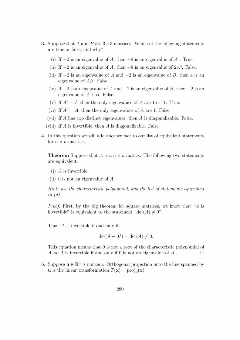
3. Suppose that A and B are 3×3 matrices. Which of the following statementsare true or false, and why?
(i) If −2 is an eigenvalue of A, then −8 is an eigenvalue of A3. True.
(ii) If −2 is an eigenvalue of A, then −8 is an eigenvalue of 2A3. False.
(iii) If −2 is an eigenvalue of A and −2 is an eigenvalue of B, then 4 is aneigenvalue of AB. False.
(iv) If −2 is an eigenvalue of A and −2 is an eigenvalue of B, then −2 is aneigenvalue of A+B. False.
(v) If A2 = I, then the only eigenvalues of A are 1 or -1. True.
(vi) If A2 = A, then the only eigenvalues of A are 1. False.
(vii) If A has two distinct eigenvalues, then A is diagonalizable. False.
(viii) If A is invertible, then A is diagonalizable. False.
4. In this question we will add another fact to our list of equivalent statementsfor n× n matrices.
Theorem Suppose that A is a n× n matrix. The following two statementsare equivalent.
(i) A is invertible.
(ii) 0 is not an eigenvalue of A.
Hint: use the characteristic polynomial, and the list of statements equivalentto (a).
Proof. First, by the big theorem for square matrices, we know that “A isinvertible” is equivalent to the statement “det(A) 6= 0”.
Thus, A is invertible if and only if
det(A− 0I) = det(A) 6= 0.
This equation means that 0 is not a root of the characteristic polynomial ofA, so A is invertible if and only if 0 is not an eigenvalue of A.
5. Suppose u ∈ Rn is nonzero. Orthogonal projection onto the line spanned byu is the linear transformation T (x) = proju(x).
280

Recall that we showed in Tutorial 6, question 4 that the matrix of this lineartransformation is given by the formula
A =1
uTuuuT .
(i) Show that 1 and 0 are eigenvalues of A by using the definition of eigen-values (find some eigenvectors for these eigenvalues). Hint: this questionmay be easier if you think about the geometric properties of proju.
Solution: The way to show that 0 and 1 are eigenvalues for A is to usethe definition and find eigenvectors.
First, observe that
Au =
(1
uTuuuT
)u =
1
uTuu(uTu) = u = 1u
so λ = 1 is an eigenvalue of A, and u is an eigenvector for this eigenvalue.
Second, if v is nonzero and orthogonal to u, then
Av =
(1
uTuuuT
)v =
1
uTuu(uTv) = 0 = 0v
so λ = 0 is an eigenvalue of A, and v is an eigenvector for this eigenvalue.
Tutorial 11: Orthogonality
Background: Chapter 11 of the lecture notes.
1. Let
S = span
1−2003
,
02101
,
10400
,
10104
⊆ R5
(i) Use Gram-Schmidt to compute an orthogonal basis for the subspace S.
Final answer: Note that the fourth vector in the set above is a lin-ear combination of the previous vectors in the set, so when performing
281

Gram-Schmidt, the vector s4 will compute to be 0 and we throw it out.
One way to write the final answer is:
(1,−2, 0, 0, 3), (1, 26, 14, 0, 17), (73,−94, 275, 0,−87).
(ii) Compute a basis for S⊥ using the fact that row(A)⊥ = null(A). Thenuse Gram-Schmidt to compute an orthogonal basis for S⊥.
After row-reducing, we see that the basic solutions are
(−32,−7, 8, 0, 6), (0, 0, 0, 1, 0).
This is already an orthogonal basis.
(iii) Use the computations from parts (a) and (b) to confirm the formula
dim(S) + dim(S⊥) = n
for this example.
We check,dim(S) + dim(S⊥) = 3 + 2 = 5.
2. Let
v =
23−114
.(i) Use the result of Question 1.(a) to compute the orthogonal projection
projS(v).
projS(v) =8
14
1−2003
+2 + 78− 14 + 4 · 17
1162
12614017
+2 · 73− 3 · 94− 275− 4 · 87
97359
73−942750−87
=1
17
244−9074
282

(I realize the numbers in this computation get a little out of hand. Wepromise not to put a problem where you have to multiply numbers thislarge on the final)
(ii) Use the formulaprojS⊥(v) = v − projS(v)
and the result from 2.(a) to compute projS⊥(v).
projS⊥(v) =
23−114
− 1
17
244−9074
=1
17
327−81−6
(iii) Check that the vectors computed in 2.(a) and 2.(b) are orthogonal.
1
17
244−9074
· 1
17
327−81−6
=1
172(2 ·32+44 ·7+(−9) ·(−8)+0+74 ·(−6)) = 0
(iv) Use the orthonormal basis for S⊥ from question 1.(b) to compute projS⊥(v)by using the definition of orthogonal projection onto the subspace S⊥
(you should get the same answer as in 2.(b)).
projS⊥(v) =2(−32) + 3(−7) + (−1)8 + 4(6)
1173
−32−7806
+1
1
00010
=1
17
327−81−6
3. Suppose that S is a subspace of Rn with dimension k. For each statement
below, say whether it is true or false. Can you explain why?
(i) dim(S⊥) = n− k.
True. This follows from the rank-nullity theorem (see the lecture notes).
283
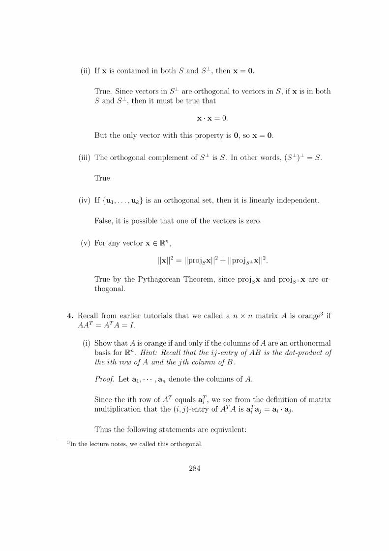
(ii) If x is contained in both S and S⊥, then x = 0.
True. Since vectors in S⊥ are orthogonal to vectors in S, if x is in bothS and S⊥, then it must be true that
x · x = 0.
But the only vector with this property is 0, so x = 0.
(iii) The orthogonal complement of S⊥ is S. In other words, (S⊥)⊥ = S.
True.
(iv) If {u1, . . . ,uk} is an orthogonal set, then it is linearly independent.
False, it is possible that one of the vectors is zero.
(v) For any vector x ∈ Rn,
||x||2 = ||projSx||2 + ||projS⊥x||2.
True by the Pythagorean Theorem, since projSx and projS⊥x are or-thogonal.
4. Recall from earlier tutorials that we called a n × n matrix A is orange3 ifAAT = ATA = I.
(i) Show that A is orange if and only if the columns of A are an orthonormalbasis for Rn. Hint: Recall that the ij-entry of AB is the dot-product ofthe ith row of A and the jth column of B.
Proof. Let a1, · · · , an denote the columns of A.
Since the ith row of AT equals aTi , we see from the definition of matrixmultiplication that the (i, j)-entry of ATA is aTi aj = ai · aj.
Thus the following statements are equivalent:
3In the lecture notes, we called this orthogonal.
284
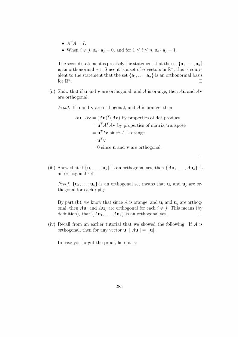
• ATA = I.
• When i 6= j, ai · aj = 0, and for 1 ≤ i ≤ n, ai · aj = 1.
The second statement is precisely the statement that the set {a1, . . . , an}is an orthonormal set. Since it is a set of n vectors in Rn, this is equiv-alent to the statement that the set {a1, . . . , an} is an orthonormal basisfor Rn.
(ii) Show that if u and v are orthogonal, and A is orange, then Au and Avare orthogonal.
Proof. If u and v are orthogonal, and A is orange, then
Au · Av = (Au)T (Av) by properties of dot-product
= uTATAv by properties of matrix transpose
= uT Iv since A is orange
= uTv
= 0 since u and v are orthogonal.
(iii) Show that if {u1, . . . ,uk} is an orthogonal set, then {Au1, . . . , Auk} isan orthogonal set.
Proof. {u1, . . . ,uk} is an orthogonal set means that ui and uj are or-thogonal for each i 6= j.
By part (b), we know that since A is orange, and ui and uj are orthog-onal, then Aui and Auj are orthogonal for each i 6= j. This means (bydefinition), that {Au1, . . . , Auk} is an orthogonal set.
(iv) Recall from an earlier tutorial that we showed the following: If A isorthogonal, then for any vector u, ||Au|| = ||u||.
In case you forgot the proof, here it is:
285

Proof. If A is orthogonal and u ∈ Rn, then
||Au|| =√
(Au) · (Au) by properties of dot-product, length
=√
(Au)T (Au) by properties of dot-product
=√
uTATAu by properties of matrix transpose
=√
uTu since A is orange
= ||u|| by properties of dot-product, length.
(v) Show that if {u1, . . . ,uk} is an orthonormal set, then {Au1, . . . , Auk}is an orthonormal set.
Proof. We already showed in part (c) that if {u1, . . . ,uk} is an orthog-onal set and A is orange, then {Au1, . . . , Auk} is an orthogonal set.
An orthonormal set is an orthogonal set with every vector a unit vector.
It remains to show that if ||ui|| = 1 for 1 ≤ i ≤ n, then ||Aui|| = 1 for1 ≤ i ≤ n.
But we know from part (d) that if A is orange, then ||Aui|| = ||ui|| = 1for 1 ≤ i ≤ n. Thus {Au1, . . . , Auk} is an orthonormal set.
286

Index
Basis, 135Basis vectors, 135
Cavalieri’s principle, 163Characteristic polynomial, 166Cofactor, 155Cofactor expansion, 155Column space, 145
Determinant, 155Diagonalizable matrix, 172Diagonalization, 172Dimension, 138distance, 90dot product, 91
Eigenspace, 168Eigenvalue, 165Eigenvector, 165elementary operations, 27elementary row operations, 29
Function, 104
Gaussian elimination, 32Gram-Schmidt algorithm, 191
Homomorphism, 161hyperplane in Rn, 100
image of a linear transformation, 115
kernel of a linear transformation, 115
leading entry, 30length, 90
linear combination, 55, 58linear equation, 14Linear transformation, 106linearly independent, 131
matrix, 26addition, 38column vector, 26entries, 26inverse, 69invertible, 67matrix product, 45matrix-vector product, 42rank, 33row vector, 26scalar multiplication, 39square matrix, 26transpose, 49zero matrix, 39
n-tuple, 17norm, 90Null space, 141Nullity, 150
orthogonal, 93Orthogonal basis, 180Orthogonal complement, 183Orthogonal set, 179Orthonormal set, 179
parallel vectors, 87, 88plane in R3, 96Projection onto a subspace, 189
287

Rank-Nullity theorem, 150Row space, 147row-echelon form, 30
set of solutionsparameter, 22
solution of a linear equation, 17span, 56Submatrix, 154subspace, 124system of linear equations, 19
associated homogeneous system, 62augmented matrix, 24basic solutions, 60coefficient matrix, 24consistent, 23constant matrix, 24homogeneous system, 57inconsistent, 23particular solution, 63solution, 19trivial solution, 57
The Subspace Test, 127
unit vector, 91
288