CSC2420 Spring 2016: Lecture 2

Allan Borodin

January 21,2016

1 / 1

Announcements and todays agendaFirst part of assignment 1 was posted last weekend. I plan to assignmore questions as we discuss additional topics. Please try to work onthe questions week by week and not postpone until the due date. Iwill set due date for assignment 1 after I assign more questions.I try to post the slides within a day or so of the lecture and usuallypost what was discussed. Some times I will post all the intendedslides for context.Todays agenda

1 Review and continue discussion of the set packing problem.2 Sketch s-set packing greedy algorithm analyis3 Abstraction of s-set packing to (s + 1)-claw free graphs.4 State O(

√m)-approximationi for set packing.

5 Priority algorithms with revocable acceptances (for packing problems).The “greedy” algorithm for weighted interval scheduling (WIS) andweighted job interval scheduling problem (WJIS).

6 Abstraction of WIS (resp. WJIS) to max independent set in chordalgraphs and (respectively) inductive 2-independent graphs.

7 Priority stack algorithms.8 The random order model. (ROM) 2 / 1

Greedy algorithms for the set packing problem

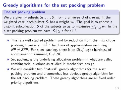
The set packing problem

We are given n subsets S1, . . . ,Sn from a universe U of size m. In theweighted case, each subset Si has a weight wi . The goal is to choose adisjoint subcollection S of the subsets so as to maximize

∑Si∈S wi . In the

s-set packing problem we have |Si | ≤ s for all i .

This is a well studied problem and by reduction from the max clique

problem, there is an m12−ε hardness of approximation assuming

NP 6= ZPP. For s-set packing, there is an Ω(s/ log s) hardness ofapproximation assuming P 6= NP.

Set packing is the underlying allocation problem in what are calledcombinatorial auctions as studied in mechanism design.

We will consider two “natural” greedy algorithms for the s-setpacking problem and a somewhat less obvious greedy algorithm forthe set packing problem. These greedy algorithms are all fixed orderpriority algorithms.

3 / 1

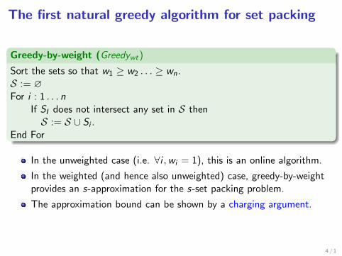
The first natural greedy algorithm for set packing

Greedy-by-weight (Greedywt)

Sort the sets so that w1 ≥ w2 . . . ≥ wn.S := ∅For i : 1 . . . n

If SI does not intersect any set in S thenS := S ∪ Si .

End For

In the unweighted case (i.e. ∀i ,wi = 1), this is an online algorithm.

In the weighted (and hence also unweighted) case, greedy-by-weightprovides an s-approximation for the s-set packing problem.

The approximation bound can be shown by a charging argument.

4 / 1

Two types of approximation arguments

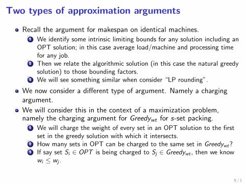
Recall the argument for makespan on identical machines.1 We identify some intrinsic limiting bounds for any solution including an

OPT solution; in this case average load/machine and processing timefor any job.

2 Then we relate the algorithmic solution (in this case the natural greedysolution) to those bounding factors.

3 We will see something similar when consider “LP rounding”.

We now consider a different type of argument. Namely a chargingargument.

We will consider this in the context of a maximization problem,namely the charging argument for Greedywt for s-set packing.

1 We will charge the weight of every set in an OPT solution to the firstset in the greedy solution with which it intersects.

2 How many sets in OPT can be charged to the same set in Greedywt?3 If say set Si ∈ OPT is being charged to Sj ∈ Greedywt , then we know

wi ≤ wj .

5 / 1

The second natural greedy algorithm for set packing

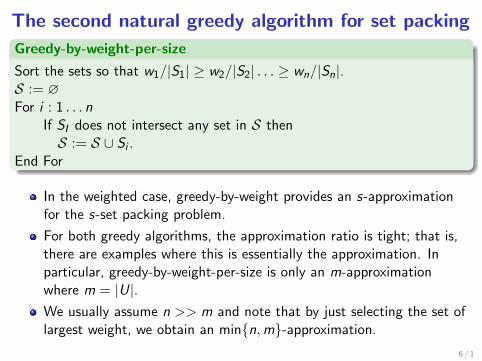
Greedy-by-weight-per-size

Sort the sets so that w1/|S1| ≥ w2/|S2| . . . ≥ wn/|Sn|.S := ∅For i : 1 . . . n

If SI does not intersect any set in S thenS := S ∪ Si .

End For

In the weighted case, greedy-by-weight provides an s-approximationfor the s-set packing problem.

For both greedy algorithms, the approximation ratio is tight; that is,there are examples where this is essentially the approximation. Inparticular, greedy-by-weight-per-size is only an m-approximationwhere m = |U|.We usually assume n >> m and note that by just selecting the set oflargest weight, we obtain an minn,m-approximation.

6 / 1

Improving the approximation for greedy set packing

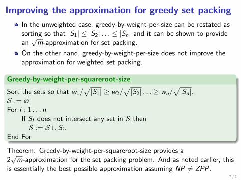
In the unweighted case, greedy-by-weight-per-size can be restated assorting so that |S1| ≤ |S2| . . . ≤ |Sn| and it can be shown to providean√m-approximation for set packing.

On the other hand, greedy-by-weight-per-size does not improve theapproximation for weighted set packing.

Greedy-by-weight-per-squareroot-size

Sort the sets so that w1/√|S1| ≥ w2/

√|S2| . . . ≥ wn/

√|Sn|.

S := ∅For i : 1 . . . n

If SI does not intersect any set in S thenS := S ∪ Si .

End For

Theorem: Greedy-by-weight-per-squareroot-size provides a2√m-approximation for the set packing problem. And as noted earlier, this

is essentially the best possible approximation assuming NP 6= ZPP.7 / 1

Another way to obtain an O(√m) approximation

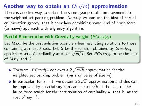
There is another way to obtain the same aysmptototic improvement forthe weighted set packing problem. Namely, we can use the idea of partialenumeration greedy; that is somehow combining some kind of brute force(or naive) approach with a greedy algorithm.

Partial Enumeration with Greedy-by-weight (PGreedyk)

Let Maxk be the best solution possible when restricting solutions to thosecontaining at most k sets. Let G be the solution obtained by Greedywtapplied to sets of cardianlity at most

√m/k . Set PGreedyk to be the best

of Maxk and G .

Theorem: PGreedyk achieves a 2√

m/k-approximation for theweighted set packing problem (on a universe of size m)

In particular, for k = 1, we obtain a 2√m approximation and this can

be improved by an arbitrary constant factor√k at the cost of the

brute force search for the best solution of cardinality k ; that is, at thecost of say nk .

8 / 1

(k + 1)-claw free graphs

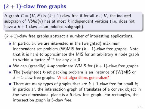
A graph G = (V ,E ) is (k + 1)-claw free if for all v ∈ V , the inducedsubgraph of Nbhd(v) has at most k independent vertices (i.e. does nothave a k + 1 claw as an induced subgraph).

(k + 1)-claw free graphs abstract a number of interesting applications.

In particular, we are interested in the (weighted) maximumindependent set problem (W)MIS for (k + 1)-claw free graphs. Notethat it is hard to approximate the MIS for an arbiitrary n node graphto within a factor n1−ε for any ε > 0.

We can (greedily) k-approximate WMIS for (k + 1)-claw free graphs.

The (weighted) k-set packing problem is an instance of (W)MIS onk + 1-claw free graphs. What algorithms generalize?

There are many types of graphs that are k + 1 claw free for small k;in particular, the intersection graph of translates of a convex object inthe two dimensional plane is a 6-claw free graph. For rectangles, theintersection graph is 5-claw free.

9 / 1

Extensions of the priority model: priority withrevocable acceptances

For packing problems, we can have priority algorithms with revocableacceptances. That is, in each iteration the algorithm can now rejectpreviously accepted items in order to accept the current item.However, at all times, the set of currently accepted items must be afeasible set and all rejections are permanent.

Within this model, there is a 4-approximation algorithm for theweighted interval selection problem WISP (Bar-Noy et al [2001], andErlebach and Spieksma [2003]), and a ≈ 1.17 inapproximation bound(Horn [2004]). More generally, the algorithm applies to the weightedjob interval selection problem WJISP resulting in an 8-approximation.

The model has also been studied with respect to the proportionalprofit knapsack problem/subset sum problem (Ye and B [2008])improving the constant approximation. And for the general knapsackproblem, the model allows a 2-approximation.

10 / 1

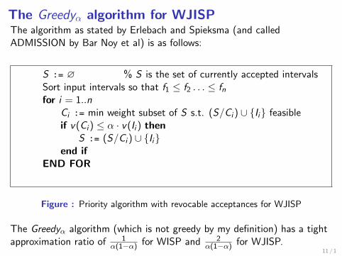
The Greedyα algorithm for WJISPThe algorithm as stated by Erlebach and Spieksma (and calledADMISSION by Bar Noy et al) is as follows:

S := ∅ % S is the set of currently accepted intervalsSort input intervals so that f1 ≤ f2 . . . ≤ fnfor i = 1..n

Ci := min weight subset of S s.t. (S/Ci ) ∪ Ii feasibleif v(Ci ) ≤ α · v(Ii ) then

S := (S/Ci ) ∪ Iiend if

END FOR

Figure : Priority algorithm with revocable acceptances for WJISP

The Greedyα algorithm (which is not greedy by my definition) has a tightapproximation ratio of 1

α(1−α) for WISP and 2α(1−α) for WJISP.

11 / 1

Priority Stack AlgorithmsFor packing problems, instead of immediate permanent acceptances,in the first phase of a priority stack algorithm, items (that have notbeen immediately rejected) can be placed on a stack. After all itemshave been considered (in the first phase), a second phase consists ofpopping the stack so as to insure feasibility. That is, while poppingthe stack, the item becomes permanently accepted if it can befeasibly added to the current set of permanently accepted items;otherwise it is rejected. Within this priority stack model (whichmodels a class of primal dual with reverse delete algorithms and aclass of local ratio algorithms), the weighted interval selectionproblem can be computed optimally.For covering problems (such as min weight set cover and min weightSteiner tree), the popping stage is insure the minimality of thesolution; that is, while popping item I from the stack, if the currentset of permanently accepted items plus the items still on the stackalready consitute a solution then I is deleted and otherwise itbecomes a permanently accepted item.

12 / 1

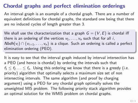
Chordal graphs and perfect elimination orderings

An interval graph is an example of a chordal graph. There are a number ofequivalent definitions for chordal graphs, the standard one being that thereare no induced cycles of length greater than 3.

We shall use the characterization that a graph G = (V ,E ) is chordal iffthere is an ordering of the vertices v1, . . . , vn such that for all i ,Nbdh(vi ) ∩ vi+1, . . . , vn is a clique. Such an ordering is called a perfectelimination ordering (PEO).

It is easy to see that the interval graph induced by interval intersection hasa PEO (and hence is chordal) by ordering the intervals such thatf1 ≤ f2 . . . ≤ fn. Using this ordering we know that there is a greedy (i.e.priority) algorithm that optimally selects a maximum size set of nonintersecting intervals. The same algorithm (and proof by chargingargument) using a PEO for any chordal graph optimally solves theunweighted MIS problem. The following priority stack algorithm providesan optimal solution for the WMIS problem on chordal graphs.

13 / 1

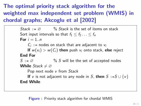
The optimal priority stack algorithm for theweighted max independent set problem (WMIS) inchordal graphs; Akcoglu et al [2002]

Stack := ∅ % Stack is the set of items on stackSort input intervals so that f1 ≤ f2 . . . ≤ fnFor i = 1..n

Ci := nodes on stack that are adjacent to viIf w(vi ) > w(Ci ) then push vi onto stack, else reject

End ForS := ∅ % S will be the set of accepted nodesWhile Stack 6= ∅

Pop next node v from StackIf v is not adjacent to any node in S , then S :=S ∪ v

End While

Figure : Priority stack algorithm for chordal WMIS14 / 1

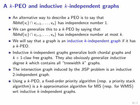
A k-PEO and inductive k-independent graphs

An alternative way to describe a PEO is to say thatNbhd(vi ) ∩ vi+1, . . . , vn has independence number 1.

We can generalize this to a k-PEO by saying thatNbhd(vi ) ∩ vi+1, . . . , vn has independence number at most k .

We will say that a graph is an inductive k-independent graph if it hasa k-PEO.

Inductive k-independent graphs generalize both chordal graphs andk + 1-claw free graphs. They also obviously generalize inductivedegree k which contains all “treewidth k” graphs.

The intersection graph induced by the JISP problem is an inductive2-independent graph.

Using a k-PEO, a fixed-order priority algorithm (resp. a priority stackalgorithm) is a k-approximation algorithm for MIS (resp. for WMIS)wrt inductive k-independent graphs.

15 / 1

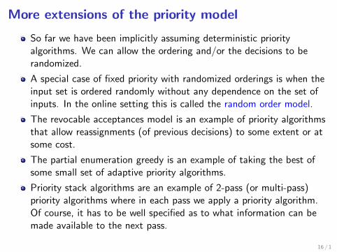
More extensions of the priority model

So far we have been implicitly assuming deterministic priorityalgorithms. We can allow the ordering and/or the decisions to berandomized.

A special case of fixed priority with randomized orderings is when theinput set is ordered randomly without any dependence on the set ofinputs. In the online setting this is called the random order model.

The revocable acceptances model is an example of priority algorithmsthat allow reassignments (of previous decisions) to some extent or atsome cost.

The partial enumeration greedy is an example of taking the best ofsome small set of adaptive priority algorithms.

Priority stack algorithms are an example of 2-pass (or multi-pass)priority algorithms where in each pass we apply a priority algorithm.Of course, it has to be well specified as to what information can bemade available to the next pass.

16 / 1

The random order model (ROM)

Motivating the random order model

The random order model provides a nice compromise between the oftenunrealistic negative results for worst case (even randomized) onlinealgorithms and the often unrealistic positive setting of inputs beinggenerated by simple distributions.

In many online scenarios, we do not have realistic assumptions as tothe distributional nature of inputs (so we default to worst caseanalysis). But in many applications we can believe that inputs doarrive randomly or more precisely uniformly at random.

The ROM can be (at least) traced back to what is called the(classical) secretary (aka marriage or dowry) problem, popularized ina Martin Gardner Scientific American article.

As Fiat et al (SODA 2015) note, perhaps Johannes Kepler(1571-1630) used some secretary algorithm when interviewing 11potential brides over two years.

17 / 1

The secretary problem

The classical problem (which has now been extended and studied in manydifferent variations is as follows:

The classic problem (as in the Gardiner article) assumes anadversarially chosen set of distinct values for (say N) items that arrivein random order (e.g. candidates for a position, offers for a car, etc.).N is assumed to be known.

Once an item (e.g. secretary) is chosen, that decision is irrevocable.Hence, this boils down to finding an optimal stopping rule, a subjectthat can be considered part of stochastic optimization.

The goal is to select one item so as to maximize the probability thatthe item chosen is the one of maximum value.

For any set of N values, maximizing the probability of choosing thebest item immediately yields a bound for the expected (over therandom orderings) value of the chosen item. For an “ordinalalgorithm”, these two measures are essentially the same. Why?

18 / 1

The secretary problem continued

It is not difficult to show that any deterministic or randomized(adversarial order) online algorithm has competitive ratio 1 at mostO( 1

N ). Hence the need to consider the ROM model to obtain moreinteresting (and hopefully more meaningful) results.

We note (and this holds more generally) that “positive results” forthe ROM model subsume the stochastic optimization scenario whereinputs are generated by an unknown (and hence known) i.i.d. process.Why?

There are many variations and extensions of the secretary problemsome of which we will consider later (or at least mention).

In general, any online problem can be studied with respect to theROM model.

1Recall that for maximization problems, competitive and approximation ratios cansometimes presented as fractions α = ALG

OPT≤ 1 and sometimes as ratios c = OPT

ALG≥ 1. I

will try to follow the convention mainly used in each application.19 / 1

The optimal stopping rule for the classical secretaryproblem

The amusing history of the secretary problem and the following result istaken up by Ferguson in a 1989 article.

Theorem: For N and r , there is an exact formula for the probability ofselecting the maximum value item after observing the first r items, andthen selecting the first item (if any) that exceeds the value of the itemsseen thus far. In the limit as N →∞, the optimal stopping rule is toobserve (i.e. not take) the first r = N/e items. The probability ofobtaining the best item is then 1/e and hence the expected value of theitem chosen is at least 1

e vmax .

20 / 1

Variations and extensions of the secretary problem

Instead of maximizing the probability of choosing the best item, wecan maximize the expected rank of the chosen item.

Perhaps the most immediate extension is to be choosing k elements.

This has been generalized to the matroid secretary problem byBabaioff. For arbitrary matroids, the approximation ratio remains anopen problem.

Another natural extension is to generalize the selection of one item tothe online (and ROM) edge weighted bipartite matching problem,where say N = |L| items arrive online to be matched with items in R.In online matching the goal is usually to maximize the size (for theunweighted case) or weight of a maximum matching.

I will next to discuss online matching and then later (hopefully) theextension to the adwords problem where the online nodes L representadvertisers/bidders with budgets and preferences/values for the Rnodes representing keywords/queries.

21 / 1

The unweighted bipartite matching problem

Before leaving (for now) online, ROM and priority algorithms, I want tobriefly discuss one more (surprising) ROM algorithm (equivalently for thisalgorithm, a randomized online algorithm) that has generated a good dealof recent research.

Let G = (U,V ,E ) be an unweighted bipartite graph with edgesE ⊂ U × V . Lets say that the vertices in U are the online verticesthat arrive one at a time u1, . . . un, revealing the offline nodes in V towhich they are adjacent.

The online algorithm must irrecvocably decide whether and how tomatch ui to an unmatched v ∈ V (if there is such a node).

It is easy to see that any greedy algorithm (i.e. one that matcheseach ui if possible) produces a maximal matching and hence is a12 -approximation (following the convention here for using fractionalapproximation ratios). This is also a tight bound for any deterministiconline algorithm as can be seen by a simple 2× 2 bipartite graph.

22 / 1

The Karp, Vazirani, Varizani (KVV) algorithm

The KVV Ranking algorithm chooses a random permutation of thenodes in V and then when a node u ∈ U appears, it matches u to thehighest ranked unmatched v ∈ V such that (u, v) is an edge (if sucha v exists).

Aside: making a random choice for each u is still only a 12 approx.

The analysis of this algorithm can be used to show that there is adeterministic greedy algorithm in the ROM model.

That is, let v1, . . . , vn be any fixed ordering of the vertices and letthe nodes in U enter randomly, then match each u to the firstunmatched v ∈ V according to the fixed order.

To argue this, consider fixed orderings of U and V ; the claim is thatthe matching will be the same whether U or V is entering online.

23 / 1

The KVV result and recent progress

KVV Theorem

Ranking provides a (1− 1/e) ≈ .63 approximation.

Original analysis is not rigorous.

There is an alternative proof (and extension) by Goel and Mehta[2008], and other proofs (e.g. in Birnbaum and Mathieu [2008]).

KVV show that the (1− 1/e) bound is essentially tight for anyrandomized online (i.e. adversarial input) algorithm. In the ROMmodel, Goel and Mehta state inapproximation bounds of 3

4 (fordeterministic) and 5

6 (for randomized) algorithms.

In the ROM model, Karande, Mehta, Tripathi [2011] show thatRanking achieves approximation at least .653 (beating 1− 1/e) andno better than .727.

24 / 1