UNIVERSITY OF OKLAHOMA

GRADUATE COLLEGE

Q ESTIMATE USING SPECTRAL DECOMPOSITION

A THESIS

SUBMITTED TO THE GRADUATE FACULTY

in partial fulfillment of the requirements for the

Degree of

MASTER OF SCIENCE

By

TOAN DAONorman, Oklahoma

2013

Q ESTIMATE USING SPECTRAL DECOMPOSITION

A THESIS APPROVED FOR THECONOCO PHILLIPS SCHOOL OF GEOLOGY AND GEOPHYSICS

BY

Dr. Kurt J. Marfurt, Chair

Dr. G. Randy Keller

Dr. Tim Kwiatkowski

c© Copyright by TOAN DAO 2013All Rights Reserved.

ACKNOWLEDGEMENTS

This thesis would not have been possible without my adviser, Dr. Kurt J.

Marfurt for giving me all the support, guidance and freedom to explore an ocean

of knowledge without getting lost. From him I started to truly understand that

learning is a lifetime process. When I complained about the new generations of

students not adequately equipped with a solid foundation of the basic science,

his response was: ”You never will have all the technical skills you will need.

Just watch me at 62 years old learning C++. Who would have thought I’d be

learning my twelfth computer language?”. Thank you for these words. I will

carry them for many years ahead.

I would like to thank Dr. Tim Kwiatkowski and Dr. G. Randy Keller for

their advice, encouragement and hours of code debugging. I would also like

to send my special thanks Dr. Vikram Jayaram for helping me look into the

problems with a different view and in the completion of the important writing

process.

I owe my deepest gratitude to my family and all my friends.

Last but not least, I would like to thank the sponsors to the Attribute-

Assisted Seismic Processing and Interpretation consortium for their financial

support.

iv

TABLE OF CONTENTS

1 INTRODUCTION 1

1.1 Motivation . . . . . . . . . . . . . . . . . . . . . . . . . . . . . . 1

1.2 Previous work . . . . . . . . . . . . . . . . . . . . . . . . . . . . 1

1.3 Hypothesis . . . . . . . . . . . . . . . . . . . . . . . . . . . . . . 2

2 THEORY 3

2.1 Definitions and terminology . . . . . . . . . . . . . . . . . . . . 3

2.2 The effect of attenuation on a seismic pulse . . . . . . . . . . . . 5

2.3 The attenuation-dispersion relation . . . . . . . . . . . . . . . . 7

2.4 The effect of attenuation on seismic data . . . . . . . . . . . . . 9

2.5 Q estimation using the spectral ratio method . . . . . . . . . . . 13

2.6 Q estimation using the average frequency method . . . . . . . . 14

3 SPECTRAL DECOMPOSITION 15

3.1 Spectral decomposition using the Continuous Wavelet Transform 15

3.2 Singularities and the Maxima Wavelet Matrix . . . . . . . . . . 15

3.3 Spectral decomposition using the maxima modulus lines with a

matching pursuit scheme . . . . . . . . . . . . . . . . . . . . . . 16

4 Q ESTIMATION USING SPECTRAL DECOMPOSITION 34

4.1 Spectral decomposition techniques for Q estimation . . . . . . . 34

4.2 Data pre-conditioning . . . . . . . . . . . . . . . . . . . . . . . 37

4.3 Principal Component Analysis . . . . . . . . . . . . . . . . . . . 38

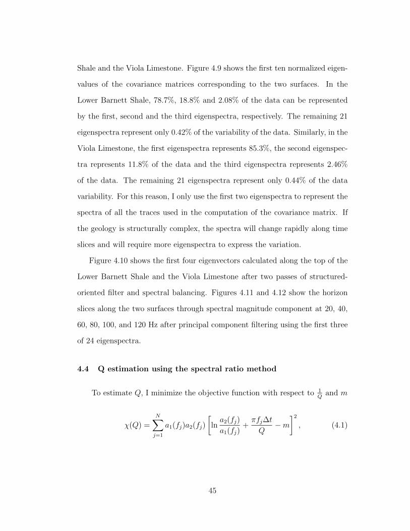
4.4 Q estimation using the spectral ratio method . . . . . . . . . . . 45

v

4.5 Application and Discussion . . . . . . . . . . . . . . . . . . . . . 51

5 CONCLUSIONS 56

REFERENCES 58

A THE CONTINUOUS WAVELET TRANSFORM 60

A.1 Definitions . . . . . . . . . . . . . . . . . . . . . . . . . . . . . . 60

A.2 The CWT applied to spectral analysis . . . . . . . . . . . . . . 61

A.3 The Morlet wavelet . . . . . . . . . . . . . . . . . . . . . . . . . 62

B PRINCIPAL COMPONENT ANALYSIS 64

C GRAPHICAL USER INTERFACES 66

C.1 The aaspi spec cwt GUI . . . . . . . . . . . . . . . . . . . . . . 66

C.2 The aaspi complex stratal slice GUI . . . . . . . . . . . . . . . . 68

C.3 The aaspi complex pca spectra GUI . . . . . . . . . . . . . . . . 70

vi

LIST OF FIGURES

2.1 (a) Seismic pulse at times t = 0.5, 1.0, 1.5, 2.0, 2.5 s, constant

Q = 2 and (b) seismic pulse at time t = 1.0s with different values

of Q. Note that the attenuation operator does not modify the

phase such that energy can arrive before t = 0 s. . . . . . . . . . 6

2.2 (a) The temporal waveform of the Dirac delta function from the

origin after traveling a distance of z = 500 m with the reference

velocity of v0 = 5000 m/s in an attenuating medium with causal-

ity taken into account for Q = 30, v0 = 5000 m/s and f0 = 30

Hz and (b) its spectral maginitude. The area between the curve

and 1 represents the amount of energy loss. . . . . . . . . . . . . 10

2.3 A 2D line through seismic amplitude data (a) without Q compen-

sation and (b) with Q compensation. The yellow arrows indicate

the reservoirs (after Wang, 2008). . . . . . . . . . . . . . . . . . 11

2.4 A 2D line through acoustic impedance computed from seismic

data (a) without Q compensation and (b) with Q compensation

(after Wang, 2008). . . . . . . . . . . . . . . . . . . . . . . . . . 12

3.1 A (a) representative seismic data trace, d(t), (b) its spectral mag-

nitude components co-rendered with the maxima modulus lines

(ridges), (c) its spectral phase components c(t, f), (d) the real

part of the J=17 composite wavelets generated by integrating

over the ridges and (e) the imaginary part of the J=17 compos-

ite wavelets generated by integrating over the ridges. . . . . . . 17

vii

3.2 Vertical slices of spectral decompositions at frequencies 20 Hz, 40

Hz, 60 Hz, 80 Hz, 100 Hz and 120 Hz. . . . . . . . . . . . . . . . 18

3.3 The magnitude spectra of the real and imaginary ridges that are

associated with the strongest events of the signal in Figure 3.1. . 19

3.4 Flowchart of the matching pursuit algorithm. . . . . . . . . . . 22

3.5 The original signal and its reconstruction after 1 through 10 iter-

ations. The J=17 MML wavelets (the real part), w(t) shown in

Figure 3.1d were used for the first iteration, approximating the

major characteristics and overall amplitude of the input data.

The number, location, and the form of the wavelets changes with

each iteration, such that the model converges to the input signal. 23

3.6 The magnitude spectra of the original signal and its reconstruc-

tion after 1 through 10 iterations using the real part of the max-

ima wavelets. . . . . . . . . . . . . . . . . . . . . . . . . . . . . 24

3.7 The original signal and its residual after 1 through 10 iterations. 25

3.8 The L-2 norm of the reconstructed signals and residuals at iter-

ations 1 through 10 using the real part of the maxima wavelet

matrix. . . . . . . . . . . . . . . . . . . . . . . . . . . . . . . . . 26

3.9 The original signal and its reconstruction after 1 through 10 it-

erations. The J=17 MML wavelets (the imaginary part), w(t)

shown in Figure 3.1e were used for the first iteration, approx-

imating the major characteristics and overall amplitude of the

input data. The number, location, and the form of the wavelets

changes with each iteration, such that the model converges to the

input signal. . . . . . . . . . . . . . . . . . . . . . . . . . . . . . 27

viii

3.10 The magnitude spectra of the original signal and its reconstruc-

tion after 1 through 10 iterations using the imaginary part of the

maxima wavelets. . . . . . . . . . . . . . . . . . . . . . . . . . . 28

3.11 The L-2 norm of the reconstructed signals and residuals at it-

erations 1 through 10 using the imaginary part of the maxima

wavelet matrix. . . . . . . . . . . . . . . . . . . . . . . . . . . . 29

3.12 A vertical slice through (a) seismic amplitude data and the data

reconstruction after (b) one, (c) three, (d) five and (e) seven and

(f) nine iterations using the real part of the maxima wavelet matrix. 30

3.13 A vertical slice through (a) seismic amplitude data and the resid-

ual data after (b) one, (c) three, (d) five and (e) seven and (f)

nine iterations using the real part of the maxima wavelet matrix. 31

3.14 A vertical slice through (a) seismic amplitude data and the data

reconstruction after (b) one, (c) three, (d) five and (e) seven

and (f) nine iterations using the imaginary part of the maxima

wavelet matrix. . . . . . . . . . . . . . . . . . . . . . . . . . . . 32

3.15 A vertical slice through a) seismic amplitude data and the resid-

ual data after (b) one, (c) three, (d) five and (e) seven and (f)

nine iterations using the real part of the maxima wavelet matrix. 33

4.1 (a) A single realization of the P-wave velocity and its correspond-

ing seismic signal, the spectra of the signal using (b) Short-Time

Fourier Transform, (c) Gabor transform, (d) S-transform and (e)

Continuous Wavelet Transform (After Reine et al., 2009). . . . . 35

ix

4.2 The theoretical and estimated Q of (a) the realization plotted in

Figure 4.1 and (b) the mean of 20 realizations using four different

spectral decomposition techniques. The variable-window trans-

forms have a better and stable match to the models (After Reine

et al., 2009). . . . . . . . . . . . . . . . . . . . . . . . . . . . . . 36

4.3 A representative vertical slice through (a) the original prestack

time migrated seismic amplitude volume, (b) the seismic ampli-

tude data after two passes of structure-oriented filtering using a

110 by 110 ft circular 5-trace window by 10 ms (11 samples) and

(c) the rejected noise volume computed by subtracting the data

shown in Figure 4.3b from that shown in Figure 4.3a. . . . . . . 39

4.4 A representative time slice through (a) the original prestack time

migrated seismic amplitude volume, (b) the seismic amplitude

data after two passes of SOF and (c) the rejected noise volume

computed by subtracting the data shown in Figure 4.4b from that

shown in Figure 4.4a. . . . . . . . . . . . . . . . . . . . . . . . . 40

4.5 A representative time slice through (a) the original prestack time

migrated seismic amplitude volume and (b) the seismic amplitude

data after two passes of SOF and spectral whitening. . . . . . . 41

4.6 Vertical slices through spectral components at (a) 20, (b) 40, (c)

60, (d) 80, (e) 100, and (f) 120 Hz computed from the data shown

in Figure 4.5b after two passes of SOF and spectral balancing.

Note that the frequency response is similar in the 20-100 Hz range

but falls off at 120 Hz. . . . . . . . . . . . . . . . . . . . . . . . 42

x

4.7 Time slices at t=1.3 s through the spectral magnitude compo-

nents at (a) 20, (b) 40, (c) 60, (d) 80, (e) 100, and (f) 120 Hz

computed from the data shown in Figure 4.4b after SOF and

spectral balancing. . . . . . . . . . . . . . . . . . . . . . . . . . 43

4.8 Horizons slices along the top Lower Barnett Shale horizon through

spectral magnitude components at (a) 20, (b) 40, (c) 60, (d) 80,

(e) 100, and (f) 120 Hz. . . . . . . . . . . . . . . . . . . . . . . 44

4.9 First five normalized eigenvalues of the covariance matrix corre-

sponding to the top of the Lower Barnett Shale and the Viola

Limestone. . . . . . . . . . . . . . . . . . . . . . . . . . . . . . . 46

4.10 The real and imaginary parts of the first four eigenvectors calcu-

lated along the top of the (a), (b) Lower Barnett Shale and (c),

(d) the Viola Limestone after two passes of SOF and spectral

balancing. . . . . . . . . . . . . . . . . . . . . . . . . . . . . . . 47

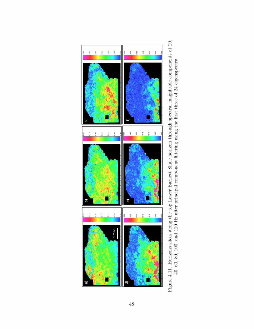
4.11 Horizons slices along the top Lower Barnett Shale horizon through

spectral magnitude components at 20, 40, 60, 80, 100, and 120

Hz after principal component filtering using the first three of 24

eigenspectra. . . . . . . . . . . . . . . . . . . . . . . . . . . . . . 48

4.12 Horizons slices along the top Viola Limestone horizon through

spectral magnitude components at 20, 40, 60, 80, 100, and 120

Hz after principal component filtering using the first three of 24

eigenspectra. . . . . . . . . . . . . . . . . . . . . . . . . . . . . . 49

4.13 (a) Normalized spectra at two points on the top of the Lower

Barnett Shale and Viola Limestone and (b) log of their spectral

ratio. The red line indicates the trend of the curve. . . . . . . . 52

xi

4.14 (a) Vertical slice of the seismic amplitude data, time structure

map of the top of (b) the Lower Barnett Shale and (c) the Viola

Limestone. . . . . . . . . . . . . . . . . . . . . . . . . . . . . . . 54

4.15 Quality factor Q computed between the top of the Lower Barnett

Shale and top of the Viola limestone using equation 4.10 . . . . 55

4.16 (a) Synthetic tuning model and (b) its corresponding ICWT de-

convolution (after Matos and Marfurt, 2011). . . . . . . . . . . . 55

A.1 A Morlet wavelet with β = 1.15, fc = 3.0 Hz. . . . . . . . . . . . 63

A.2 The spectrum of the Morlet wavelet in Figure A.1. . . . . . . . . 63

C.1 Q estimation flow chart. . . . . . . . . . . . . . . . . . . . . . . 67

C.2 The aaspi spec cwt GUI. . . . . . . . . . . . . . . . . . . . . . 69

C.3 The aaspi spec cwt GUI. . . . . . . . . . . . . . . . . . . . . . 69

C.4 The aaspi complex stratal slice GUI. . . . . . . . . . . . . . 70

C.5 The aaspi complex pca spectra GUI. . . . . . . . . . . . . . 71

xii

ABSTRACT

Attenuation is an important seismic property, especially in exploration seis-

mology since it greatly influences seismic data quality. As the industry is shifting

to explore ever thinner reservoirs, better understanding of attenuation can help

to improve the data quality as well as characterize rock properties and reservoir

heterogeneity.

Because of its capability to detect local changes, spectral decomposition

using the Continuous Wavelet Transform can be used to quantify the quality

factor Q (reciprocal of attenuation) over a seismic interval which for the case

of this study will be between the top and the base of the Lower Barnett Shale.

I introduce an improvement over the previously developed Inverse Continuous

Wavelet Transform deconvolution. The maxima modulus lines (ridges) created

by connecting the singularities obtained from spectral decomposition identify

the strongest and the most continuous events. The maxima wavelet matrix

formed by integrating along the maxima lines make up the basis functions to

model the signal. A residual signal is obtained to which we can apply the same

process to iteratively update the model. The modeled signal converges such

that the strongest and most continuous information is updated first. This algo-

rithm attempts to overcome two limitations of the Inverse Continuous Wavelet

Transform deconvolution (Matos and Marfurt, 2011) that the amplitude of the

reconstructed data is not preserved while only the largest events are represented

and smaller amplitude events are removed.

Variable-window transforms decompose the data into frequency bands amenable

to Q estimation using the spectral ratio technique. Before estimating Q, I pre-

xiii

condition the data using two passes of structured-oriented filter and spectral bal-

ancing. To furthermore enhance the signal-to-noise ratio, I use horizon-based

Principal Component Analysis (PCA) to uncorrelate the spectral component

data. The computed Q values are unrealistic due to the previous processing

workflow and complexity of the geology.

xiv

Chapter 1

INTRODUCTION

1.1 Motivation

Seismic attenuation is one of the most fundamental mechanisms of elastic

waves propagating through the earth. There are two coupled processes associ-

ated with attenuation: dissipation and dispersion. The dissipation process sup-

presses the seismic amplitude while the dispersion process distorts the phases.

Attenuation acts as a time-variant low-pass filter with a monotonically increas-

ing phase spectrum. The direct consequence of these processes on seismic data

is that the seismic wavelet becomes more stretched and its amplitude becomes

exponentially smaller with time and depth. These processes also contribute to

the non-stationary behavior of the seismic wavelet and decreasing resolution

with time and depth. As we explore for ever thinner and more subtle hydro-

carbon reservoirs, improving the resolution by compensating for attenuation

becomes more important. Furthermore, attenuation, if quantified, can be used

as a seismic attribute to characterize rock properties, reservoir heterogeneity

and the success of completion processes.

1.2 Previous work

Work on wave attenuation can be found in early literature in different fields,

especially in physics and chemistry. Some of the most recent work to estimate Q

includes Tonn (1991) who estimates attenuation using both time and frequency

methods, and by Singleton et al. (2006) who decomposes the data using Gabor

1

wavelets. Wang (2008) attempts to correct for the attenuation effect rather than

estimating it. His inverse filters correct for amplitude, phase or both at the same

time. Van der Baan (2012) considers the inverse filter a bandwidth enhancement

process that can be approximated by time-varying Wiener deconvolution.

Chapter 2 summarizes the theory of attenuation. Chapter 3 introduces spec-

tral decomposition and data reconstruction using the maxima modulus line with

a matching pursuit scheme. Chapter 4 shows how to precondition the the spec-

tral components using complex Principal Component Analysis. These filtered

data are then used to estimate Q using an iteratively reweighted least-squares

spectral ratio method. Chapter 5 summarizes the results and discusses limita-

tion of the method.

1.3 Hypothesis

The Fourier Transform measures the global periodicity of a signal resulting

in coefficients for a suite of sines and cosines spanning the entire length of the

seismic trace. The Continuous Wavelet Transform, on the other hand, uses the

concept of a temporarily-windowed mother wavelet that is scaled, translated

down the trace and then correlated with the signal to detect local changes with

respect to time. Since attenuation changes the amplitude and phase of the

signal with time, the Continuous Wavelet Transform can be used to estimate

and compensate for attenuation effects.

2

Chapter 2

THEORY

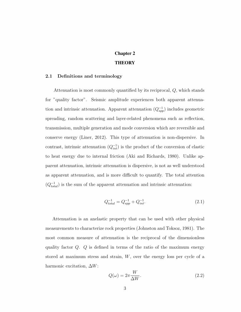
2.1 Definitions and terminology

Attenuation is most commonly quantified by its reciprocal, Q, which stands

for ”quality factor”. Seismic amplitude experiences both apparent attenua-

tion and intrinsic attenuation. Apparent attenuation (Q−1app) includes geometric

spreading, random scattering and layer-related phenomena such as reflection,

transmission, multiple generation and mode conversion which are reversible and

conserve energy (Liner, 2012). This type of attenuation is non-dispersive. In

contrast, intrinsic attenuation (Q−1int) is the product of the conversion of elastic

to heat energy due to internal friction (Aki and Richards, 1980). Unlike ap-

parent attenuation, intrinsic attenuation is dispersive, is not as well understood

as apparent attenuation, and is more difficult to quantify. The total attention

(Q−1total) is the sum of the apparent attenuation and intrinsic attenuation:

Q−1total = Q−1

app +Q−1int. (2.1)

Attenuation is an anelastic property that can be used with other physical

measurements to characterize rock properties (Johnston and Toksoz, 1981). The

most common measure of attenuation is the reciprocal of the dimensionless

quality factor Q. Q is defined in terms of the ratio of the maximum energy

stored at maximum stress and strain, W , over the energy loss per cycle of a

harmonic excitation, ∆W :

Q(ω) = 2πW

∆W. (2.2)

3

The attenuation coefficient α is defined in terms of Q using Kolsky’s (1955)

Q model:

α =ω

2v

1

Q(ω), (2.3)

where ω is the temporal frequency measured in radian/s and v is the phase

velocity.

The amplitude A is proportional to W 1/2. Assuming Q >> 1, equation 2.2

can be rewritten in term of the ratio between the change in amplitude, ∆A over

the amplitude, A:

1

Q(ω)=

1

π

∆A

A. (2.4)

The amplitude A decreases by πQ

in one period T = 2πω

. Therefore, the amplitude

at time t, A(t), can be written as

A(t) = A0(1− π

Q)n, (2.5)

where A0 is the amplitude at time t = 0 and n = ωt2π

is the number of periods.

Taking the limit as ωt→∞ gives:

A(t) = A0e− ωt

2Q . (2.6)

Replacing t = xv

to obtain the amplitude as a function of distance gives

A(x) = A0e− ωx

2vQ . (2.7)

Equations 2.6 and 2.7 show that amplitude decreases exponentially with time

and distance.

4

2.2 The effect of attenuation on a seismic pulse

Consider a delta function as a seismic pulse traveling with velocity v along

the x axis in a viscoelastic medium characterized by the function Q(z, ω). To

be able to derive the shape of the pulse at time t, I decompose the pulse into

Fourier components

U(z, ω) =

∫R

δ(t− z

v)eiωtdt = e

iωzv . (2.8)

The pulse u(z, t) at time t and location z is reconstructed by summing all the

Fourier components after applying Q(z, ω) using equation 2.7:

u(z, t) =1

2π

∫R

e−ωz

2vQ(z,ω)U(z, ω)e−iωtdω. (2.9)

Equation 2.9 does not have an analytic expression if Q(z, ω) is an arbitrary

function. To simplify the calculation, I assume Q(z, ω) be a constant. Equation

2.9 now can be expressed as

u(z, t) =1

π

z2vQ

( z2vQ

)2 + ( zv− t)2

. (2.10)

The pulse u(z, t) at the same time t and location z is plotted in Figure 2.1

for different values of Q at different times. The shape of the pulse at time t is

dictated by the value of Q. Lower values of Q (higher attenuation) will decrease

the amplitude and broaden the wavelet. Higher values of Q (lower attenuation)

will keep the amplitude and shape of the wavelet closer to the shape of the

original pulse. An exponential curve can be fit to be tangential to all the

peaks of the pulse, which is in agreement with the behavior of the amplitude

5

Fig

ure

2.1.

(a)

Sei

smic

puls

eat

tim

est

=0.

5,1.

0,1.

5,2.

0,2.

5s,

const

antQ

=2

and

(b)

seis

mic

puls

eat

tim

et

=1.

0sw

ith

diff

eren

tva

lues

ofQ

.N

ote

that

the

atte

nuat

ion

oper

ator

does

not

modif

yth

ephas

esu

chth

aten

ergy

can

arri

veb

efor

et

=0

s.

6

in equation 2.7. Aki and Richards (1980) indicate that this constant-Q model

is physically not possible because a pulse at any given time t > 0 and Q 6= ∞

can respond to the stress before it arrives, violating the causality principle.

To address this problem, Q(z, ω) must be a function of ω. In general, higher

frequencies will be attenuated faster and travel faster than lower frequencies.

2.3 The attenuation-dispersion relation

Let u(z, t) be a vertically traveling plane wave at at position z and time t,

u(z, t) =

∫S0(ω)ei(ωt−kz)dω (2.11)

where k is the wavenumber and S0(ω) is the source wavelet in the frequency

domain. In an attenuating medium, k is a complex number

k =ω

v(ω)+ iα(ω) = kr(1 +

i

2Q(ω)), (2.12)

where α(ω) is the attenuation factor, Q(ω) is the quality factor and v(ω) is the

phase velocity.

Futterman (1962) shows that attenuation and dispersion must be coupled

such that u(x, t) responds after the stress is applied at the source location.

Using this result to guarantee the causality of the system, Aki and Richards

(1980) derive the relationship connecting frequency ω, phase velocity v(ω) and

attenuation factor α(ω) to guarantee u(z, t) = 0 before the earliest possible

arrival time t = zv∞

,

ω

v(ω)=

ω

v∞+ H[α(ω)], (2.13)

where he defines v∞ = limω→∞

v(ω) and the operator H denotes the Hilbert trans-

7

form. The phase of u(z, t) depends on the the Hilbert transform of the atten-

uation factor α(ω) which involves all the frequencies, giving rise to alternative

Q models.

Q models for the phase velocity include Kolsky’s (1955) constant-Q model,

Strick’s (1967) power law model, Kjartansson’s (1979) model, Muller’s (1983)

model, Azimi et al.’s (1968) second and third model, the Cole-Cole (1941) model

and the standard linear solid. Wang and Guo (2004) show that it is possible

to modify the parameters of Kolsky’s (1955) model to match the other mod-

els. Ursin and Toverud (2004) examined all these models and found all were

equivalent in the 10-100 Hz seismic spectrum. All the Q models discussed re-

quire a reference phase velocity, v0 and a reference frequency, ω0. For instance,

Futterman (1962) proposes a term γF

k =ω

v0

[1− 1

πQln(

ω

ω0

)] =ω

v0

γF , (2.14)

while Kjartansson (1979) models the wavenumber differently using γK

k =ω

v0

(ω

ω0

)−1πQ =

ω

v0

γK . (2.15)

Substituting one of the above expressions for the wavenumber k into equation

2.11 gives

u(t, t0) =

∫S0(ω)exp

[iω(t0γ − t)

]exp(− ωt0γ

2Q

)dω, (2.16)

where γ takes one of the functions γF or γK .

Equation 2.16 can be rewritten in term of the inverse Fourier transform of a

8

function:

u(t, t0) = F−1[S0(ω)exp

(iωt0γ

)exp(− ωt0γ

2Q

)](2.17)

The first exponential term in equation 2.17 models the phase while the second

exponential term models the amplitude of the wavelet. The reference phase

velocity and frequency serve as a standard to compare the behavior at all other

frequencies. For simplicity, let the source wavelet s(t) = δ(t), S(ω) = 1, Q = 30,

v∞ = 6250 m/s, v0 = 5000 m/s and f0 = 30 Hz. Using equation 2.17 with

Futterman’s model, I obtain the temporal waveform and the spectral magnitude

of the pulse at z = 500 m and plot them in Figure 2.2. The shape of the pulse

spreads but dies out before time t = zv∞

= 0.08 s.

2.4 The effect of attenuation on seismic data

The earth acts as a low-pass filter in which the higher frequency components

are suppressed more than the lower frequency components. This phenomenon

causes a number of issues in seismic exploration as high frequencies are as im-

portant as low frequencies. First of all, attenuation lowers the seismic data

quality if the high frequency components of the data fall below the noise level.

Figure 2.3a shows a 2D line after acoustic inversion from seismic data without Q

compensation. Figure 2.3b shows the same 2D line after acoustic inversion from

data with Q compensation. In both figures, the white vertical lines outline the

well log. The strata in Figure 2.3b match the well-log data better than those in

Figure 2.3a. We immediately notice that Figure 2.3 contains higher frequencies

and therefore shows more detail. Some of the structures are imaged better in

this figure such as a fault at x = 13 km and t = 4.0 s. In Figure 2.3, this fault

is more difficult to see since part of the high frequency data are missing.

9

Fig

ure

2.2.

(a)

The

tem

por

alw

avef

orm

ofth

eD

irac

del

tafu

nct

ion

from

the

orig

inaf

ter

trav

elin

ga

dis

tance

ofz

=50

0m

wit

hth

ere

fere

nce

velo

city

ofv 0

=50

00m

/sin

anat

tenuat

ing

med

ium

wit

hca

usa

lity

take

nin

toac

count

forQ

=30

,v 0

=50

00m

/san

df 0

=30

Hz

and

(b)

its

spec

tral

mag

init

ude.

The

area

bet

wee

nth

ecu

rve

and

1re

pre

sents

the

amou

nt

ofen

ergy

loss

.

10

Fig

ure

2.3.

A2D

line

thro

ugh

seis

mic

amplitu

de

dat

a(a

)w

ithou

tQ

com

pen

sati

onan

d(b

)w

ithQ

com

pen

sati

on.

The

yellow

arro

ws

indic

ate

the

rese

rvoi

rs(a

fter

Wan

g,20

08).

11

Fig

ure

2.4.

A2D

line

thro

ugh

acou

stic

imp

edan

ceco

mpute

dfr

omse

ism

icdat

a(a

)w

ithou

tQ

com

pen

sati

onan

d(b

)w

ithQ

com

pen

sati

on(a

fter

Wan

g,20

08).

12

Figures 2.4 shows another example by Wang (2008) that demonstrates the

effect of Q on seismic data. The reservoir indicated by the yellow arrows is better

imaged with Q compensation. Part of the reservoir on the right of Figure 2.4a

cannot be imaged or interpreted with the same confidence as that in Figure 2.4b.

Through the Q compensation process, the frequency bandwidth is broadened

and the waveform is squeezed and more symmetric.

2.5 Q estimation using the spectral ratio method

The spectral ratio method is a robust frequency-domain method to estimate

Q. Given two points x1, x2 and their magnitude spectra a1(f), a2(f), Q is

calculated between the two points by comparing the energy of the signal at all

the available frequencies. For each frequency f , a2(f) can be expressed in terms

of a1(f) and Q as:

a2(f) = g(z1, z2)a1(f)exp(−πf∆z

Qv

)(2.18)

where ∆z = z2 − z1 and g(z1, z2) is a frequency-independent function incor-

porating the effects of spherical divergence, dependence of the pulse amplitude

on impedance, source strength, recorder gain and angular dependence of the

radiation pattern (Costag and Ernest, 1987).

Taking the natural logarithm of both side of equation 2.18 gives

lna2(f)

a1(f)= ln g(z1, z2)− πf∆z

Qv. (2.19)

or in terms of travel time:

13

lna2(f)

a1(f)= ln g(t1, t2)− πf∆t

Q. (2.20)

Cross-plotting ln a2(f)a1(f)

versus frequency f yields a linear relationship whose slope

is p = −π∆zQv

= −π∆tQ

, from which Q can be calculated.

2.6 Q estimation using the average frequency method

In an attenuating medium, the frequency spectrum of a wavelet is contin-

uously changing where the amount of change is a function of Q. Treating f as

a random variable with probability density function, a2(f), Hauge (1981) finds

the average frequency,

f =

∫fa2(f)df, (2.21)

and variance

σ2f =

∫(f − f)2a2(f)df (2.22)

of the spectrum to be related by

df

dz= − 2π

Qvσ2f , (2.23)

or in terms of travel time:

df

dt= −2π

Qσ2f . (2.24)

In practice, spectral ratio methods are more commonly used and are more

robust than the average frequency method.

14

Chapter 3

SPECTRAL DECOMPOSITION

3.1 Spectral decomposition using the Continuous Wavelet Trans-

form

The Continuous Wavelet Transform introduced by Morlet et al. (1982) is

one of the more popular techniques used in spectral decomposition, breaking

broadband seismic data into its time-frequency components. The mathematics

of the Continuous Wavelet Transform is summarized in Appendix A.

Figures 3.1 show a representative seismic signal and its spectral magnitude

and phase computed using the complex Morlet wavelets. A vertical slice of the

spectrum describes the behavior of a particular frequency over time. Likewise

a horizontal slice is the frequency profile at that specific time. The magnitude

spectrum indicates that the frequencies range from 10-80 Hz and are localized

at t = 1.30, 1.36, 1.40 and 1.45 seconds. Figure 3.2 shows a suite of frequency

components of a vertical slice of the data. Note that the variation in each of the

magnitude components can be observed. The vertical slice through the original

data is shown in Figure 3.14a.

3.2 Singularities and the Maxima Wavelet Matrix

Mallat (2009) defined singularities in the complex time-frequency domain,

c(j, f), as the local maxima of the magnitude of the CWT coefficients along

the time axis (Figure 3.1b). Mallat (2009) noted that singularities associated

with the spectral peaks form ridges in the time-frequency domain, which when

15

convolved with the corresponding wavelet and summed represent the more im-

portant features of the original input seismic trace. Rather than use the corre-

sponding wavelet at each frequency component to reconstruct the data, Matos

and Marfurt (2011) convolved the maximum modulus lines (ridges) (MML)

with a broader band wavelet, thereby extending the bandwidth of the data,

resulting in what they called inverse continuous wavelet transform deconvolu-

tion (ICWTD). There are two limitations of both Mallat (2009) and Matos

and Marfurt’s (2011) algorithms. First, the amplitude of the reconstruction is

not preserved, while second, only the largest events are represented, such that

smaller amplitude but perhaps important events are removed.

The maxima wavelet matrix, W, is formed by integrating along the sets of

connected singularities (ridges) after placing the center of the wavelet ψf,τ (t) at

each singularity. W forms the basis for the input signal d where the jth column

wj is localized about the time of the jth ridge. In general, the singularities fall

between discrete samples. Although assigning the ridges for purposes of QC to

the nearest sample such as shown in Figures 3.1d and e are adequate for display

purposes, a more accurate estimate will improve the temporal resolution of the

maxima wavelet matrix. I therefore fit a parabola between c(tj−1, f), c(tj, f)

and c(tj+1, f) about each peak to obtain the peak time at a fractional sample

values prior to summation.

3.3 Spectral decomposition using the maxima modulus lines with a

matching pursuit scheme

Figure 3.4 demonstrates the flowchart of the matching pursuit algorithm

to decompose the data into the ridge components. I modify Mallat’s (2009)’s

16

Fig

ure

3.1.

A(a

)re

pre

senta

tive

seis

mic

dat

atr

ace,

d(t)

,(b

)it

ssp

ectr

alm

agnit

ude

com

pon

ents

co-r

ender

edw

ith

the

max

ima

modulu

slines

(rid

ges)

,(c

)it

ssp

ectr

alphas

eco

mp

onen

tsc(t,f

),(d

)th

ere

alpar

tof

theJ

=17

com

pos

ite

wav

elet

sge

ner

ated

by

inte

grat

ing

over

the

ridge

san

d(e

)th

eim

agin

ary

par

tof

theJ

=17

com

pos

ite

wav

elet

sge

ner

ated

by

inte

grat

ing

over

the

ridge

s.

17

Fig

ure

3.2.

Ver

tica

lsl

ices

ofsp

ectr

aldec

omp

osit

ions

atfr

equen

cies

20H

z,40

Hz,

60H

z,80

Hz,

100

Hz

and

120

Hz.

18

Figure 3.3. The magnitude spectra of the real and imaginary ridges that areassociated with the strongest events of the signal in Figure 3.1.

19

workflow by convolving and summing the appropriate wavelets along the MMLs,

ridge by ridge, forming a composite wavelet for each of the J ridges (3.1d and

e). I then least-squares fit the J composite wavelets to the input data, forming

a modeled (fit) trace, and a residual (error) trace. The standard least-squares

solution to minimize the objective function g(x) = ||rk −Mx||2 is given by

x = (MTM + εI)−1MT rk, (3.1)

where x is the vector that contains the coefficients of the maxima wavelets, ε is

a small preconditioning factor and I is the identity matrix.

This process is repeated, with each iteration operating on the residual of the

previous iteration, updating the modeled data trace until the process converges

to an acceptably small residual. This algorithm has many similarities to match-

ing pursuit (e.g. Liu and Marfurt, 2007) except that in this paper the locations

of the wavelets fall along the ridges of a suite of spectral components rather

than at the peak envelope of the undecomposed input or residual trace. Figure

3.5 shows the original time domain signal and its reconstruction after one to ten

iterations using the real part of the maxima wavelet matrix. Figure 3.7 shows

the frequency spectra of the original signal and each of the reconstruction.

Figure 3.9 shows the original time domain signal and its reconstruction after

one to ten iterations using the imaginary part of the maxima wavelet matrix.

Figure 3.10 shows the frequency spectra of the original signal and each of the

reconstruction. Figure 3.14 shows a representative vertical line through the

original seismic data and its data reconstruction after one, three and five itera-

tions. The first iteration is Matos et al.’s (2011) ICWTD. While converging to

the original data, the reconstructed data reject the steeply dipping noise.

20

Using the real part of the maxima wavelet matrix to reconstruct the data is

better than the imaginary part because the input data is zero-phase and the real

part of the maxima wavelet matrix associated with the real part of the Morlet

wavelet matches with the zero-phase data better. Similarly, the imaginary part

of the maxima wavelet matrix associated with the imaginary part of the Morlet

wavelet is out of phase with the zero-phase data.

21

Figure 3.4. Flowchart of the matching pursuit algorithm.

22

Fig

ure

3.5.

The

orig

inal

sign

alan

dit

sre

const

ruct

ion

afte

r1

thro

ugh

10it

erat

ions.

TheJ

=17

MM

Lw

avel

ets

(the

real

par

t),w

(t)

show

nin

Fig

ure

3.1d

wer

euse

dfo

rth

efirs

tit

erat

ion,

appro

xim

atin

gth

em

ajo

rch

arac

teri

stic

san

dov

eral

lam

plitu

de

ofth

ein

put

dat

a.T

he

num

ber

,lo

cati

on,

and

the

form

ofth

ew

avel

ets

chan

ges

wit

hea

chit

erat

ion,

such

that

the

model

conve

rges

toth

ein

put

sign

al.

23

Fig

ure

3.6.

The

mag

nit

ude

spec

tra

ofth

eor

igin

alsi

gnal

and

its

reco

nst

ruct

ion

afte

r1

thro

ugh

10it

erat

ions

usi

ng

the

real

par

tof

the

max

ima

wav

elet

s.

24

Fig

ure

3.7.

The

orig

inal

sign

alan

dit

sre

sidual

afte

r1

thro

ugh

10it

erat

ions.

25

Figure 3.8. The L-2 norm of the reconstructed signals and residuals atiterations 1 through 10 using the real part of the maxima wavelet matrix.

26

Fig

ure

3.9.

The

orig

inal

sign

alan

dit

sre

const

ruct

ion

afte

r1

thro

ugh

10it

erat

ions.

TheJ

=17

MM

Lw

avel

ets

(the

imag

inar

ypar

t),w

(t)

show

nin

Fig

ure

3.1e

wer

euse

dfo

rth

efirs

tit

erat

ion,

appro

xim

atin

gth

em

ajo

rch

arac

teri

stic

san

dov

eral

lam

plitu

de

ofth

ein

put

dat

a.T

he

num

ber

,lo

cati

on,

and

the

form

ofth

ew

avel

ets

chan

ges

wit

hea

chit

erat

ion,

such

that

the

model

conve

rges

toth

ein

put

sign

al.

27

Fig

ure

3.10

.T

he

mag

nit

ude

spec

tra

ofth

eor

igin

alsi

gnal

and

its

reco

nst

ruct

ion

afte

r1

thro

ugh

10it

erat

ions

usi

ng

the

imag

inar

ypar

tof

the

max

ima

wav

elet

s.

28

Figure 3.11. The L-2 norm of the reconstructed signals and residuals atiterations 1 through 10 using the imaginary part of the maxima wavelet

matrix.

29

Fig

ure

3.12

.A

vert

ical

slic

eth

rough

(a)

seis

mic

amplitu

de

dat

aan

dth

edat

are

const

ruct

ion

afte

r(b

)on

e,(c

)th

ree,

(d)

five

and

(e)

seve

nan

d(f

)nin

eit

erat

ions

usi

ng

the

real

par

tof

the

max

ima

wav

elet

mat

rix.

30

Fig

ure

3.13

.A

vert

ical

slic

eth

rough

(a)

seis

mic

amplitu

de

dat

aan

dth

ere

sidual

dat

aaf

ter

(b)

one,

(c)

thre

e,(d

)five

and

(e)

seve

nan

d(f

)nin

eit

erat

ions

usi

ng

the

real

par

tof

the

max

ima

wav

elet

mat

rix.

31

Fig

ure

3.14

.A

vert

ical

slic

eth

rough

(a)

seis

mic

amplitu

de

dat

aan

dth

edat

are

const

ruct

ion

afte

r(b

)on

e,(c

)th

ree,

(d)

five

and

(e)

seve

nan

d(f

)nin

eit

erat

ions

usi

ng

the

imag

inar

ypar

tof

the

max

ima

wav

elet

mat

rix.

32

Fig

ure

3.15

.A

vert

ical

slic

eth

rough

a)se

ism

icam

plitu

de

dat

aan

dth

ere

sidual

dat

aaf

ter

(b)

one,

(c)

thre

e,(d

)five

and

(e)

seve

nan

d(f

)nin

eit

erat

ions

usi

ng

the

real

par

tof

the

max

ima

wav

elet

mat

rix.

33

Chapter 4

Q ESTIMATION USING SPECTRAL DECOMPOSITION

4.1 Spectral decomposition techniques for Q estimation

The output of spectral decomposition serves as the input to estimate Q.

There are as many techniques to estimate Q as methods of decomposition.

Reine et al. (2009) create 1D frequency-dependent stochastic model whose

Vp = 2000 m/s, ρ = 2100 kg/m3, standard deviation of Vp, σv = 7.5%, and

standard deviation of the incompressibility fluctuations, σk = 15%.

Figure 4.1 show one realization of the transmitted signal and its spectral de-

composition using Short-Time window Fourier Transform, the Gabor transform,

the S-transform and the Continuous Wavelet Transform. Figure 4.2a shows the

frequency-dependent Q of the realization in Figure 4.1.

20 realizations of the model are generated and decomposed into frequency

bands using four different methods. Figure 4.2b shows the theoretical and mean

measured 1/Q profiles. From the experiments, Reine et al. (2009) conclude that

the attenuation measurements made by variable-window continuous wavelet

transform and S-transform are both more stable and give stronger match to

the model than the fixed window Fourier Transform. Based on this result, I will

attempt to compute Q using the Continuous Wavelet Transform technique that

I develop in Chapter 3.

34

Fig

ure

4.1.

(a)

Asi

ngl

ere

aliz

atio

nof

the

P-w

ave

velo

city

and

its

corr

esp

ondin

gse

ism

icsi

gnal

,th

esp

ectr

aof

the

sign

alusi

ng

(b)

Shor

t-T

ime

Fou

rier

Tra

nsf

orm

,(c

)G

abor

tran

sfor

m,

(d)

S-t

ransf

orm

and

(e)

Con

tinuou

sW

avel

etT

ransf

orm

(Aft

erR

eine

etal

.,20

09).

35

Figure 4.2. The theoretical and estimated Q of (a) the realization plotted inFigure 4.1 and (b) the mean of 20 realizations using four different spectral

decomposition techniques. The variable-window transforms have a better andstable match to the models (After Reine et al., 2009).

36

4.2 Data pre-conditioning

The target area is contaminated with the steeply dipping high frequency

noise which I interpret to be migration operator aliasing. Before estimating

Q, I apply structure-oriented filter (SOF) to the data. Figure 4.3a shows a

representative vertical slice through the original prestack time migrated seis-

mic amplitude volume. Figure 4.3b shows the same slice after two passes of

structure-oriented filtering using a 110 by 110 ft circular 5-trace window by 10

ms (11 samples). Much of the high-frequency dipping noise cutting across the

relatively flat has been rejected. Figure 4.3c shows the rejected noise computed

by subtracting the data shown in Figure 4.3b from that shown in Figure 4.3a.

Note that the rejected noise is higher frequency but spatially chaotic and not

correlated to geology. Figures 4.4 show a representative time slice at t = 1.3 s

through the original seismic amplitude data, the filtered data and the rejected

noise. Note that the short wavelength ”checkboard” noise cutting across the

relatively flat reflectors that correspond to the migration aliasing artifacts seen

previously in Figure 4.3a is filtered out.

The structure-oriented filtered seismic amplitude data shown in 4.3b are then

spectrally whitening within a 5-130 Hz window, with a preconditioning of 4%.

Figures 4.5 show a representative time slice through the original prestack time

migrated seismic amplitude volume and the seismic amplitude data after two

passes of SOF and spectral whitening. The white arrows indicate thin reflectors

in the target area that are better resolved. Figures 4.6 show vertical slices

through spectral components at 20, 40, 60, 80, 100, and 120 Hz computed from

the data shown in Figure 4.5b after two passes of SOF and spectral balancing.

Note that the frequency response is similar in the 20-100 Hz range but falls off at

37

120 Hz. Figures 4.7 show time slices at t=1.3 s through the spectral magnitude

components at 20, 40, 60, 80, 100, and 120 Hz computed from the data shown

in Figure 4.4b after SOF and spectral balancing. Figures 4.8 show horizons

slices along the top Lower Barnett Shale horizon through spectral magnitude

components at 20, 40, 60, 80, 100, and 120 Hz.

4.3 Principal Component Analysis

Seismic data are noisy such that we need to condition our data before using

the Q estimation methods I introduced in chapter 2. First, I need to interpolate

the complex spectra along user defined surfaces. Specifically, I interpolate real

and imaginary components along a suite of stratal slices (Appendix C). Next I

filter the spectra of the two surfaces using Principal Component Analysis, an

orthogonal linear transformation that estimates the correlation between mea-

surements. There are a number of methods to implement the PCA algorithm.

In this thesis, I use the one described by Guo et al. (2009), which is summarized

in Appendix B.

Given the spectra of a data volume, each frequency component represents a

measurement. The measurements are normalized to zero-mean, then input to

the PCA algorithm. If the spectra along a given horizon or stratal slice have

the same shape, they will be completely defined by the first eigenspectrum.

Eigenspectra that are associated with second, third, forth, and so on largest

eigenvalues reveal variations in the spectra that are critical to the Q estimation

algorithm.

Figure 4.10 shows the real and the imaginary parts of the first five eigen-

spectra of the covariance matrices computed along the top of the Lower Barnett

38

Figure 4.3. A representative vertical slice through (a) the original prestacktime migrated seismic amplitude volume, (b) the seismic amplitude data aftertwo passes of structure-oriented filtering using a 110 by 110 ft circular 5-tracewindow by 10 ms (11 samples) and (c) the rejected noise volume computed by

subtracting the data shown in Figure 4.3b from that shown in Figure 4.3a.

39

Figure 4.4. A representative time slice through (a) the original prestack timemigrated seismic amplitude volume, (b) the seismic amplitude data after twopasses of SOF and (c) the rejected noise volume computed by subtracting the

data shown in Figure 4.4b from that shown in Figure 4.4a.

40

Figure 4.5. A representative time slice through (a) the original prestack timemigrated seismic amplitude volume and (b) the seismic amplitude data after

two passes of SOF and spectral whitening.

41

Fig

ure

4.6.

Ver

tica

lsl

ices

thro

ugh

spec

tral

com

pon

ents

at(a

)20

,(b

)40

,(c

)60

,(d

)80

,(e

)10

0,an

d(f

)12

0H

zco

mpute

dfr

omth

edat

ash

own

inF

igure

4.5b

afte

rtw

opas

ses

ofSO

Fan

dsp

ectr

albal

anci

ng.

Not

eth

atth

efr

equen

cyre

spon

seis

sim

ilar

inth

e20

-100

Hz

range

but

falls

offat

120

Hz.

42

Fig

ure

4.7.

Tim

esl

ices

att=

1.3

sth

rough

the

spec

tral

mag

nit

ude

com

pon

ents

at(a

)20

,(b

)40

,(c

)60

,(d

)80

,(e

)10

0,an

d(f

)12

0H

zco

mpute

dfr

omth

edat

ash

own

inF

igure

4.4b

afte

rSO

Fan

dsp

ectr

albal

anci

ng.

43

Fig

ure

4.8.

Hor

izon

ssl

ices

alon

gth

eto

pL

ower

Bar

net

tShal

ehor

izon

thro

ugh

spec

tral

mag

nit

ude

com

pon

ents

at(a

)20

,(b

)40

,(c

)60

,(d

)80

,(e

)10

0,an

d(f

)12

0H

z.

44

Shale and the Viola Limestone. Figure 4.9 shows the first ten normalized eigen-

values of the covariance matrices corresponding to the two surfaces. In the

Lower Barnett Shale, 78.7%, 18.8% and 2.08% of the data can be represented

by the first, second and the third eigenspectra, respectively. The remaining 21

eigenspectra represent only 0.42% of the variability of the data. Similarly, in the

Viola Limestone, the first eigenspectra represents 85.3%, the second eigenspec-

tra represents 11.8% of the data and the third eigenspectra represents 2.46%

of the data. The remaining 21 eigenspectra represent only 0.44% of the data

variability. For this reason, I only use the first two eigenspectra to represent the

spectra of all the traces used in the computation of the covariance matrix. If

the geology is structurally complex, the spectra will change rapidly along time

slices and will require more eigenspectra to express the variation.

Figure 4.10 shows the first four eigenvectors calculated along the top of the

Lower Barnett Shale and the Viola Limestone after two passes of structured-

oriented filter and spectral balancing. Figures 4.11 and 4.12 show the horizon

slices along the two surfaces through spectral magnitude component at 20, 40,

60, 80, 100, and 120 Hz after principal component filtering using the first three

of 24 eigenspectra.

4.4 Q estimation using the spectral ratio method

To estimate Q, I minimize the objective function with respect to 1Q

and m

χ(Q) =N∑j=1

a1(fj)a2(fj)

[lna2(fj)

a1(fj)+πfj∆t

Q−m

]2

, (4.1)

45

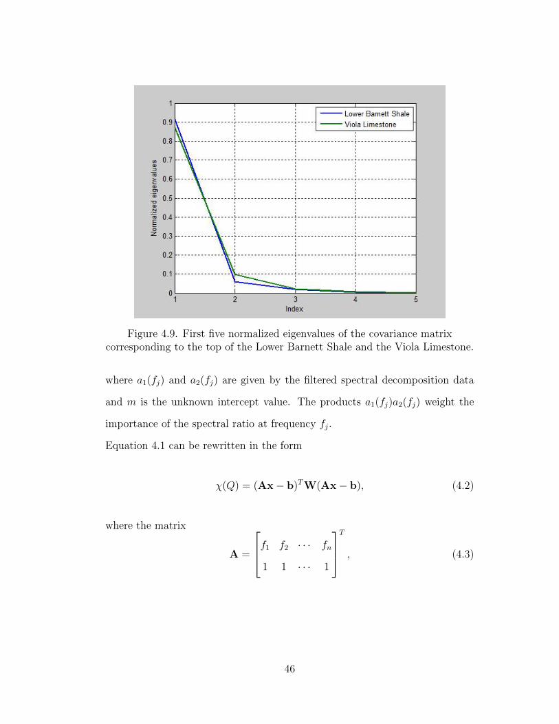
Figure 4.9. First five normalized eigenvalues of the covariance matrixcorresponding to the top of the Lower Barnett Shale and the Viola Limestone.

where a1(fj) and a2(fj) are given by the filtered spectral decomposition data

and m is the unknown intercept value. The products a1(fj)a2(fj) weight the

importance of the spectral ratio at frequency fj.

Equation 4.1 can be rewritten in the form

χ(Q) = (Ax− b)TW(Ax− b), (4.2)

where the matrix

A =

f1 f2 · · · fn

1 1 · · · 1

T

, (4.3)

46

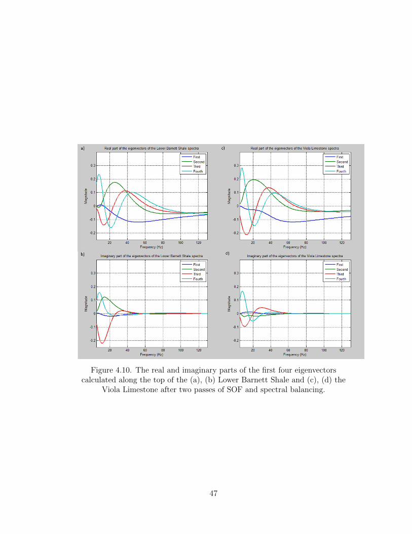
Figure 4.10. The real and imaginary parts of the first four eigenvectorscalculated along the top of the (a), (b) Lower Barnett Shale and (c), (d) the

Viola Limestone after two passes of SOF and spectral balancing.

47

Fig

ure

4.11

.H

oriz

ons

slic

esal

ong

the

top

Low

erB

arnet

tShal

ehor

izon

thro

ugh

spec

tral

mag

nit

ude

com

pon

ents

at20

,40

,60

,80

,10

0,an

d12

0H

zaf

ter

pri

nci

pal

com

pon

ent

filt

erin

gusi

ng

the

firs

tth

ree

of24

eige

nsp

ectr

a.

48

Fig

ure

4.12

.H

oriz

ons

slic

esal

ong

the

top

Vio

laL

imes

tone

hor

izon

thro

ugh

spec

tral

mag

nit

ude

com

pon

ents

at20

,40

,60

,80

,10

0,an

d12

0H

zaf

ter

pri

nci

pal

com

pon

ent

filt

erin

gusi

ng

the

firs

tth

ree

of24

eige

nsp

ectr

a.

49

the weight matrix W is an N by N diagonal matrix

W =

a1(f1)a2(f1)

a1(f2)a2(f2)

. . .

a1(fN)a2(fN)

, (4.4)

the vector

b =

[ln a2(f1)

a1(f1)ln a2(f2)

a1(f2)· · · ln a2(fn)

a1(fn)

]T, (4.5)

and the unknown vector

x =

[−π∆t

Qm

]T. (4.6)

The standard weighted least squares solution is

xw = (ATWA)−1WATb. (4.7)

To enhance the stability of the solution, I solve this optimization problem using

iteratively re-weighted least squares to remove outliners. The residual r is given

by

r = b−Axw. (4.8)

50

The new weight matrix W is an N by N diagonal matrix:

W =

11+|r1|2

11+|r2|2

. . .

11+|rN |2

. (4.9)

Minimizing the objective function but now with the weight W, the solution is

x = (ATWA)−1WATb. (4.10)

Figure 4.13 shows the filtered normalized spectra at two representative points

on the top of lower Barnett Shale and Viola Limestone.

4.5 Application and Discussion

Figure 4.14a shows a vertical slice of the seismic amplitude data rendered

with the time structure maps of the top of the Lower Barnett Shale and the Viola

Limestone. Figure 4.15 shows the computed Q map. The estimated Q values

are not correct due to a number of factors. In terms of processing, accurate Q

values require very careful processing workflow that do not dramatically alter the

frequency content of the data. In particular, stretch due to migration algorithms

introduces a distortion of the resulting spectrum. If the picked velocity is too

fast or too slow, the imaged reflector will be under or over corrected. After stack

high frequencies will be attenuated, while low frequencies will be preserved. My

data were stacked by a commercial processor so I have no quality control over

51

Figure 4.13. (a) Normalized spectra at two points on the top of the LowerBarnett Shale and Viola Limestone and (b) log of their spectral ratio. The red

line indicates the trend of the curve.

52

the velocities. If the top of the Lower Barnett is improperly imaged due to an

inaccurate velocity and if the Viola were accurately imaged, I would expect a

broad band signal at the Viola, giving rise to a negative value of Q.

The travel times at different offsets sample different geology, thereby smear-

ing any Q effect. My data are at a depth of about 7000 ft with a maximum

offset of 14000 ft. For the Lower Barnett, vertically traveling energy travels 300

ft while the far offset energy incident at 45◦ travels 420 ft, thereby suffering

greater attenuation. Q is laterally smeared over an area of 600 ft.

Rao and Wang (2009) find that attenuation is also closely associated with

fractures. Fractures smaller than or equal to a half-wavelength of seismic acts

as single diffraction points and in practice, with a limited frequency band, a

significant number of small fractures may be missed and the attenuation mea-

surement may be inaccurate. Tuning effects also give rise to spectral changes.

Figures 4.16 shows a synthetic tuning model and its ICWT deconvolution which

is close to the original model. Convolution of two opposite-sign reflection coef-

ficients that are close to each other with the source wavelet is equivalent to a

differentiator in time domain or amplifying the high frequencies.

Equal-sign reflection coefficients with the source wavelet is an integration

operator in the frequency domain which preserves the low frequencies but at-

tenuates higher frequencies. The shift from lower (Lower Barnett) to higher

peak frequency (Viola) as shown in Figure 4.13 is frequently observed in the

data and probably the result of thin beds. Such a shift produces an unrealistic

negative Q value.

53

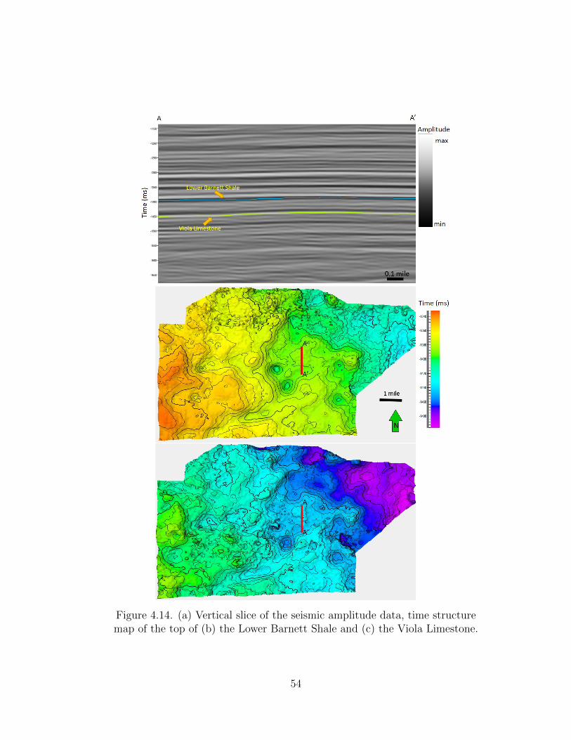
Figure 4.14. (a) Vertical slice of the seismic amplitude data, time structuremap of the top of (b) the Lower Barnett Shale and (c) the Viola Limestone.

54

Figure 4.15. Quality factor Q computed between the top of the Lower BarnettShale and top of the Viola limestone using equation 4.10 .

Figure 4.16. (a) Synthetic tuning model and (b) its corresponding ICWTdeconvolution (after Matos and Marfurt, 2011).

55

Chapter 5

CONCLUSIONS

The ridges or connected singularities obtained from the Continuous Wavelet

Transform contain the most important information in the data. The maxima

wavelet matrix derived from the ridges makes up the basis to model the data

in such a manner that the amplitude is preserved and the smaller events are

updated into the model at later iteration. The first iteration of the maxima

wavelet matching is equivalent to the Inverse Continuous Wavelet Transform

deconvolution proposed by Matos and Marfurt (2011).

Spectral decomposition using the Continuous Wavelet Transform is able to

detect the local change in amplitude and phase in greater detail and can there-

fore can be used to estimate attenuation. In principle, accurate spectral com-

ponents should provide a means to estimate Q. I applied such a workflow

to a Barnett Shale survey that was acquired after 400 wells were drilled and

completed using hydraulic fracturing. My resulting Q images are difficult to

interpret and perhaps inaccurate due to inaccurate velocities at the top and

bottom of the reservoir. If the data are of good quality, the anomalous spectral

behavior may be due to as yet poorly understood mechanics of gas charged,

fractured shale. A number of factors were addressed as to why the methods did

not work including data quality due to picking velocity, migration artifacts and

the effects on frequencies of fractures and tuning effects. In addition, wide angle

stack smears out the Q effect as the seismic wave at different offsets. A careful

processing workflow is necessary in order to not alter the frequency response of

the data and accurately estimate Q, such as high resolution velocity picking,

56

near-angle stack and non-stretch NMO.

57

REFERENCES

Aki, K., and P.G. Richards, 1980, Quantitative Seismology: Theory andMethods: W. H. Freeman & Co.

Azimi, S. A., A. V. Kalinin, V. V. Kalinin, and B. L. Pivovarov, 1968, Impulseand transient characteristics of media with linear and quadratic absorptionlaws: Izvestiya, Physics of the Solid Earth, 2, 88-93.

Cole, K. S., and R. H. Cole, 1941, Dispersion and absorption in dielectrics:I. Alternating current characteristics: Journal of Chemical Physics, 9,342-351.

Costag, G. M., and K. R. Ernest, 1987, Seismic attenuation and Poisson’sratios in oil sands from crosshole measurements: Journal of the CanadianSociety of Exploration Geophysicists, 23, 46-55.

Futterman, W. I., 1962, Dispersive body waves: Journal of Geophysical Re-search, 67, 5279-5291.

Guo, H., K. J. Marfurt, and J. Liu (2009), Principal component spectralanalysis, Geophysics, 74, 35-43.

Hauge, P., 1981, Measurements of attenuation from vertical seismic profles:Geophysics, 46, 1548-1558.

Johnston, D. H., and M. N. Toksoz, 1974, Definitions and terminology inSeismic Wave Attenuation: Geophysics Reprint Series, 2, Society of Ex-ploration Geophysics.

Kjartansson, E., 1979, Constant Q-wave propagation and attenuation: Jour-nal of Geophysical Research, 84, 4737-4748.

Kolsky, H., 1955, The propagation of stress pulses in viscoelastic solid: Philo-sophical Magazine, 1, 691-710.

Liner, C. C., 2012, Elements of Seismic Dispersion: A Somewhat PracticalGuide to Frequency-dependent Phenomena: Society of Exploration Geo-physicists.

Liu, J. L., and K. J. Marfurt, 2007, Instantaneous spectral attributes to detectchannels: Geophysics, 72, 23-31.

58

Mallat, S., 2009, A wavelet tour of signal processing: Academic Press.

Matos, M. C., and K. J. Marfurt, 2011, Inverse continuous wavelet transformdeconvolution: 81st Annual International Meeting of the SEG, ExpandedAbtracts, 1861-1865

Morlet, J., G. Arens, E. Fourgeau and D. Giard, 1982, Wave propagation andsampling theory - Part II: Sampling theory and complex waves, Geophysics,47, 222-236.

Muller, G., 1983, Rheological proporties and velocity dispersion of a mediumwith power-law dependence of Q on frequency: Journal of GeophysicalResearch, 54, 2029.

Rao, Y. and Y. Wang, Fracture effects in seismic attenuation images recon-structed by waveform tomography: Geophysics, 74, 2534.

Reine, C., M. van der Baan, and C. Roger (2009), The robustness of seismicattenuation measurements using fixed- and variable-window time-frequencytransforms: Geophysics, 74, 123-135.

Strick, E., 1967, The determination of Q, dynamic viscosity and transientcreep curves from wave propagation measurements: Geophysical Journal.Royal Astronomical Society, 13, 197-218.

Tonn, R., 1991, The determination of the seismic quality factor Q fromVSP data: A comparison of different computational methods: Geophys-ical Prospecting, 39, 1-27

Ursin, B., and T. Toverud, 2002, Comparison of seismic dispersion and atten-uation models: Studia Geophysica et Geodaetic, 46, 293-320.

Van der Baan M., 2012 Bandwidth enhancement: Inverse Q filtering or time-varying Wiener deconvolution?: Geophysics, 77, 133-142.

Wang, Y., and J. Guo, 2004, Modified Kolsky model for seismic attenuationand dispersion: Journal of Geophysics and Engineering, 1, 187-196.

Wang, Y., 2008, Seismic inverse Q Filtering: Blackwell Publishing.

59

Appendix A

THE CONTINUOUS WAVELET TRANSFORM

A.1 Definitions

The Continuous Wavelet Transform (CWT) is a time-frequency method

that decomposes a signal into duration-limited, band-passed components (Mal-

lat, 2009). Higher-frequency components are short-duration, broad-band while

low frequency components are long-duration, narrow-band signals. The CWT

is an excellent tool to analyze non-stationary seismic signal, providing useful

information of time-frequency localization. An advantage of the CWT is that

one can design a mother wavelet Ψ(t) depending on the nature of the signal

and the features one wishes to detect, provided that the wavelet satisfies the

following conditions:

1. Absolute integrability, ∫|Ψ(t)|dt <∞, (A.1)

2. Square integrability or finite energy,

∫|Ψ(t)|2dt <∞, and (A.2)

3. Admissibilty or zero DC-component,

∫Ψ(t)dt = 0. (A.3)

60

The wavelet at scale a and centered at time τ is given by

ψa,τ (t) =1√a

Ψ(t− τa

). (A.4)

The CWT of a signal d(t) is defined by:

c(a, τ) =< s,Ψa,τ >≡1√a

∫s(t)ψ∗(

t− τa

)dt, (A.5)

where ψ∗ denotes the complex conjugate of ψ.

The inverse transform is performed by integrating over all scales and delay

times:

d(t) =1

CΨ

∫c(a, b)

1√a

Ψ(t− τa

)da

a2dτ, (A.6)

where CΨ is a constant associated with the wavelet and is defined by

CΨ =

∫ +∞

0

|Ψ(ω)|2

ωdω, (A.7)

where Ψ(ω) denotes the Fourier transform of Ψ(t).

For a real signal d(t), the inverse transform can be computed as

d(t) =2

CΨ

Re[ ∫

c(a, τ)1√aψ(a, τ)

da

a2dτ]. (A.8)

A.2 The CWT applied to spectral analysis

Equations A.5 and A.8 are useful in data compression and filtering, and

are commonly used in suppressing air wave noise. As interpreters, we are also

interested in time-frequency analysis that quantifies the localization of frequen-

cies in time. To do so, given a mother wavelet with centered frequency 1Hz, I

61

replace the scale a with 1f

where f is the central frequency of the wavelet. Then

the CWT will have the form

c(f, τ) =√f

∫d(t)Ψ∗(f(t− τ))dt, (A.9)

while its corresponding inverse transform has the form

d(t) =1

CΨ

∫c(f, τ)

√fΨ(f(t− τ))dfdτ. (A.10)

A.3 The Morlet wavelet

This thesis and much CWT work use Morlet wavelets. A complex Morlet

wavelet in the time domain is given by

Ψβ,fc(t) =β√π

[exp(

2πifct)

exp(−β2t2

2

)− exp

(− 2β2

)], (A.11)

where 1β

is the standard deviation or the time-bandwidth and fc is the central

frequency of the wavelet in Hz. In practice, exp(− 2β2

)is very small for

the value of β I use that the wavelet becomes approximately but not strictly

admissible.

Figure A.1 shows a Morlet wavelet whose frequency bandwidth, β = 1.15 Hz

and the central frequency, fc = 3.0 Hz.

62

Figure A.1. A Morlet wavelet with β = 1.15, fc = 3.0 Hz.

Figure A.2. The spectrum of the Morlet wavelet in Figure A.1.

63

Appendix B

PRINCIPAL COMPONENT ANALYSIS

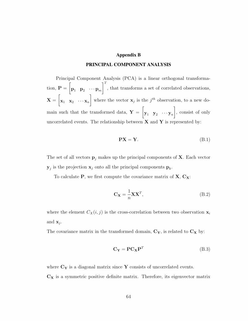
Principal Component Analysis (PCA) is a linear orthogonal transforma-

tion, P =

[p1 p2 · · ·pm

]T, that transforms a set of correlated observations,

X =

[x1 x2 · · ·xn

]where the vector xj is the jth observation, to a new do-

main such that the transformed data, Y =

[y1 y2 · · ·yn

], consist of only

uncorrelated events. The relationship between X and Y is represented by:

PX = Y. (B.1)

The set of all vectors pj makes up the principal components of X. Each vector

yj is the projection xj onto all the principal components pk.

To calculate P, we first compute the covariance matrix of X, CX:

CX =1

nXXT , (B.2)

where the element CX(i, j) is the cross-correlation between two observation xi

and xj.

The covariance matrix in the transformed domain, CY, is related to CX by:

CY = PCXPT (B.3)

where CY is a diagonal matrix since Y consists of uncorrelated events.

CX is a symmetric positive definite matrix. Therefore, its eigenvector matrix

64

V is an orthonormal matrix and satisfies VT = V−1. It can be verified that

P = V is a solution to equation B.3.

By picking P = V, P can be rewritten as the sum of weighted outer-products

of the principal components (eigenvalue decomposition):

P =m∑j=1

ejpjpTj , (B.4)

where ej is the eigenvalue associated with the eigenvector pj.

Substituting equation B.4 into equation B.1 gives:

Y =

[m∑j=1

ejpjpTj

]X. (B.5)

Without loss of generality, suppose the eigenvalues ej’s are sorted in descending

order e1>e2> · · ·>em>0. Then define Yk to be the partial sum of Y:

Yk =

[k∑j=1

ejpjpTj

]X. (B.6)

In practice, assuming that the large variance is associated with important struc-

tures and small variance is associated with noise, limiting the number of terms

in the sum is a filter that enhances the SNR.

PCA can be extended to apply to complex data. The mathematics is the

same as for real data, except the covariance matrix of X, CX, is a self-adjoint

matrix: CX = CHX.

65

Appendix C

GRAPHICAL USER INTERFACES (GUIs)

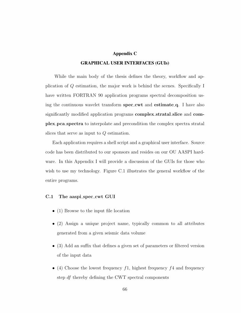
While the main body of the thesis defines the theory, workflow and ap-

plication of Q estimation, the major work is behind the scenes. Specifically I

have written FORTRAN 90 application programs spectral decomposition us-

ing the continuous wavelet transform spec cwt and estimate q. I have also

significantly modified application programs complex stratal slice and com-

plex pca spectra to interpolate and precondition the complex spectra stratal

slices that serve as input to Q estimation.

Each application requires a shell script and a graphical user interface. Source

code has been distributed to our sponsors and resides on our OU AASPI hard-

ware. In this Appendix I will provide a discussion of the GUIs for those who

wish to use my technology. Figure C.1 illustrates the general workflow of the

entire programs.

C.1 The aaspi spec cwt GUI

• (1) Browse to the input file location

• (2) Assign a unique project name, typically common to all attributes

generated from a given seismic data volume

• (3) Add an suffix that defines a given set of parameters or filtered version

of the input data

• (4) Choose the lowest frequency f1, highest frequency f4 and frequency

step df thereby defining the CWT spectral components

66

Figure C.1. Q estimation flow chart.

67

• (5) Check the box if you want the output spectral magnitude and/or phase

as a 4D cube in the order t, f, cdp no, line no

• (6) Check the box if you want the output magnitude components

• (7) Check the box if you want the output phase components

• (8) Click to change the tab to modify MPI and other less commonly

modified variables

• (9) Check the box if you wish to use MPI

• (10) Enter the number of processors per node

• (11) Enter the list of nodes, separated by blanks. Default=localhost

• (12) Check the box if you want verbose output for debugging

• (13) Enter the range for output inline and crossline ranges.

C.2 The aaspi complex stratal slice GUI

• (1) Browse to the 4D spectral magnitude and spectral phase volume pre-

viously generated by program spec cwt or spec cmp

• (2) Browse to input the upper and lower stratal surfaces saved in Earth

Vision format.

• (3) Define the number of output slices, minimum is 2

• (4) Enter an unique project name and suffix

• (5) Enter times to either include or exclude the waveform along the picked

horizons. A positive value will be added to the horizon.

68

Figure C.2. The aaspi spec cwt GUI.

Figure C.3. The aaspi spec cwt GUI.

69

Figure C.4. The aaspi complex stratal slice GUI.

C.3 The aaspi complex pca spectra GUI

• (1) Browse and find the spectral magnitude and spectral phase stratal

slice input files

• (2) Enter a unique project name and suffix

• (3) Start time and end time will be read automatically from the input files

• (4) Enter the lowest and highest frequency (in Hz) to be analyzed

• (5) Enter number of principle components to generate

• (6) Check the boxes for output file options.

70

Figure C.5. The aaspi complex pca spectra GUI.

71