Embed Size (px)
Citation preview

UNIVERSITY OF OKLAHOMA
GRADUATE COLLEGE
IMPROVING FAULT IMAGES USING A DIRECTIONAL LAPLACIAN OF A
GAUSSIAN OPERATOR
A THESIS
SUBMITTED TO THE GRADUATE FACULTY
in partial fulfillment of the requirements for the
Degree of
MASTER OF SCIENCE
By
GABRIEL MACHADO ACOSTA
Norman, Oklahoma
2016

IMPROVING FAULT IMAGES USING A DIRECTIONAL LAPLACIAN OF A
GAUSSIAN OPERATOR
A THESIS APPROVED FOR THE
CONOCOPHILLIPS SCHOOL OF GEOLOGY AND GEOPHYSICS
BY
______________________________
Dr. Kurt Marfurt, Chair
______________________________
Dr. Roger Slatt
______________________________
Dr. John Pigott

© Copyright by GABRIEL MACHADO ACOSTA 2016
All Rights Reserved.

To my dear family, and those friends that more than friends, but are like family to me.
To all of you.

iv
Acknowledgements
I would like to thank the sponsors of the Attribute-Assisted Seismic Processing
and Interpretation Consortium for their guidance and financial support. I would also like
to thank Schlumberger for providing Petrel licenses used in the current research paper.
Finally, the NZPAM for providing access to their data to the geoscience community at
large.

v
Table of Contents
Acknowledgements .............................................................................................................. iv
List of Figures ....................................................................................................................... vi
Abstract ................................................................................................................................. xi
Chapter 1: Directional Laplacian of a Gaussian theory ...................................................... 1
Eigenvector estimation of fault dip and azimuth .................................................... 1
Fault smoothing and edge enhancement using the directional Laplacian of a
Gaussian operator ......................................................................................... 3
Directional smoothing and sharpening .................................................................... 4
Chapter 2: dLoG application on two New Zealand basins ................................................. 7
Great South Basin...................................................................................................... 7
Canterbury Basin ..................................................................................................... 16
Chapter 3: dLoG as a preconditioner for ant-tracking and automatic fault picking ........ 22
The ant-tracking algorithm ..................................................................................... 22
Fault object extraction............................................................................................. 32
Chapter 4: Conclusions ....................................................................................................... 39
References ............................................................................................................................ 40
Appendix: Geologic Background of the Great South Basin ............................................. 42

vi
List of Figures
Figure 1. Cartoon showing reflectors (as solid red lines) and a coherence anomaly (as
black dotted line). The analysis window (in green) is a circle centered on the analysis
point (in orange). The eigenvector v3 is perpendicular to the fault plane reflector (blue
arrow), while the normal vector n is perpendicular to the reflector (red arrow). The
dLoG operator (red negative and blue positive) is short in the direction parallel to v3 and
three times longer in the direction parallel to v1 and v2 ...................................................... 5
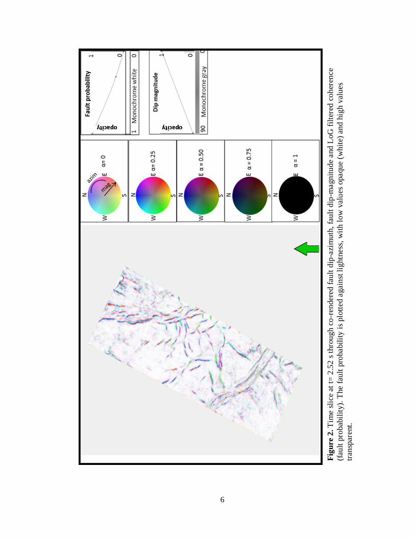
Figure 2. Time slice at t= 2.52 s through co-rendered fault dip-azimuth, fault dip-
magnitude and LoG filtered coherence (fault probability). The fault probability is
plotted against lightness, with low values opaque (white) and high values transparent. .. 6
Figure 3. (a) Time slice at t=2.52 s and (b) vertical slice along AA' through a seismic
amplitude volume with a bin size of 12.5 by 25 m.............................................................. 8
Figure 4. (a) Time slice at t=2.52 s and (b) vertical slice along AA' through a coherence
volume computed from the seismic amplitude data shown in Figure 3. The orientation
of the coherence anomalies in (a) are shown on Figure 2. .................................................. 9
Figure 5. (a) Time slice at t=2.52 s and (b) vertical slice along AA' through the
directional dLoG attribute computed from the coherence volume shown in Figure 5. (c)
Filter applied to coherence computed from the dip magnitude of v3 that suppresses
features parallel to reflector dip. Block blue arrows indicate faults that are now more
continuous and easier to identify. ....................................................................................... 11
Figure 6. Time slice at t=2.52 s through co-rendered fault dip-azimuth, fault dip-
magnitude, fault probability and seismic amplitude. The fault dip magnitude and
azimuth are computed from v3. The opacity used for each attribute is displayed on top

vii
of the color bar. Fault dip azimuth is plotted against a cyclical color bar, fault dip
magnitude against a monochrome gray scale, the dLoG attribute against a monochrome
white scale and seismic amplitude against a black and white binary color bar. Fault dip
azimuth and magnitude can be easily characterized through this combination of
attributes. Sharpened events sub parallel to the vertical slices appear smeared (blue and
yellow on the N-S line, red and green on the E-W line). .................................................. 13
Figure 7. (a) Time slice at t= 2.8 s through co-rendered fault dip-azimuth, fault dip-
magnitude, fault probability and seismic amplitude. The fault dip magnitude and
azimuth are computed from v3. The opacity used for each attribute is displayed on top
of the color bar. Fault dip azimuth is plotted against a cyclical color bar, fault dip
magnitude against monochrome gray the fault probability attribute against monochrome
white and seismic amplitude against a black and white dipole color bar. Shale
dewatering features are pointed with the blue block arrow. (b) and (c) show two vertical
lines with orthogonal orientation and the seismic image of the shale dewatering features
with an outward dipping trend. ........................................................................................... 15
Figure 8. Time slice at t=2.04 s through a) coherence, b) dLoG of coherence fault
probability c) co-rendered fault dip-azimuth, fault dip-magnitude and dLoG of
coherence (“fault” probability). The fault dip magnitude and azimuth are computed
from v3. The transparency function used for each attribute is displayed on top of the
color bar. Fault dip azimuth is plotted against a cyclical color bar, fault dip magnitude
against a monochrome gray color bar, fault probability against a monochrome white
color bar. Channel features are easily recognized through the conventional coherence,

viii
but sharpened and cleaner after dLoG filtering. The channel edges are further
characterized by combining with fault dip magnitude and azimuth attributes. ............... 17
Figure 9. Time slice at t= 2.52 s through faults shown in Figure 6 highlighting near
horizontal discontinuities through the use of a taper which hinders any feature with a
dip greater than 25°.............................................................................................................. 18
Figure 10. Time slice at t= 2.52 s through faults corresponding to Figure 6 with a dip
magnitude filter that reflects features whose dip is less than 65°. .................................... 19
Figure 11. 3D view of two vertical lines through the seismic amplitude volume, and a
box probe through co-rendered fault dip azimuth and fault dip magnitude showing
polygonal faulting. The fault probability modulates the opacity, where vowels with
α<0.5 are being rendered transparent. Lineaments that are less than 25° of dip to the
reflector have been filtered out. .......................................................................................... 20
Figure 12. The same image as Figure 11, but now with faults with N and S azimuths
rendered transparent. Thus a synthetic and antithetic fault system is highlighted .......... 21
Figure 13. A model of how real ants find the shortest path. (a) Ants arrive at a decision
point. (b) Some ants choose the upper path and some the lower path. The choice is
random. (c) Since the ants move at approximately a constant speed, the ants that choose
the lower, shorter, path reach the opposite decision point faster than those that choose
the upper, longer, path. (d) Pheromone accumulates at a higher rate on the shorter path
due to a higher amount of ants crossing it. The number of dashed lines is approximately
proportional to the amount of pheromone deposited by ants (taken from Dorigo et al.,
1997). .................................................................................................................................... 23

ix
Figure 14. (a) Time slice through a fault attribute (variance) with (b) corresponding ant
tracking results (after Iske et al., 2005). ............................................................................. 24
Figure 15. Seismic amplitude of survey from the Taranaki Basin. Relatively flat
geology on top of normally faulted sequences below 1500 ms. Block arrow indicates an
unconformity. ....................................................................................................................... 25
Figure 16. The same vertical section from Figure 15 through (a) variance attribute and
(b) corresponding ant-tracked attribute. The stereonet shows that ants were constrained
to search within a cone of 30° about the vertical (fault dips > 60°). ................................ 26
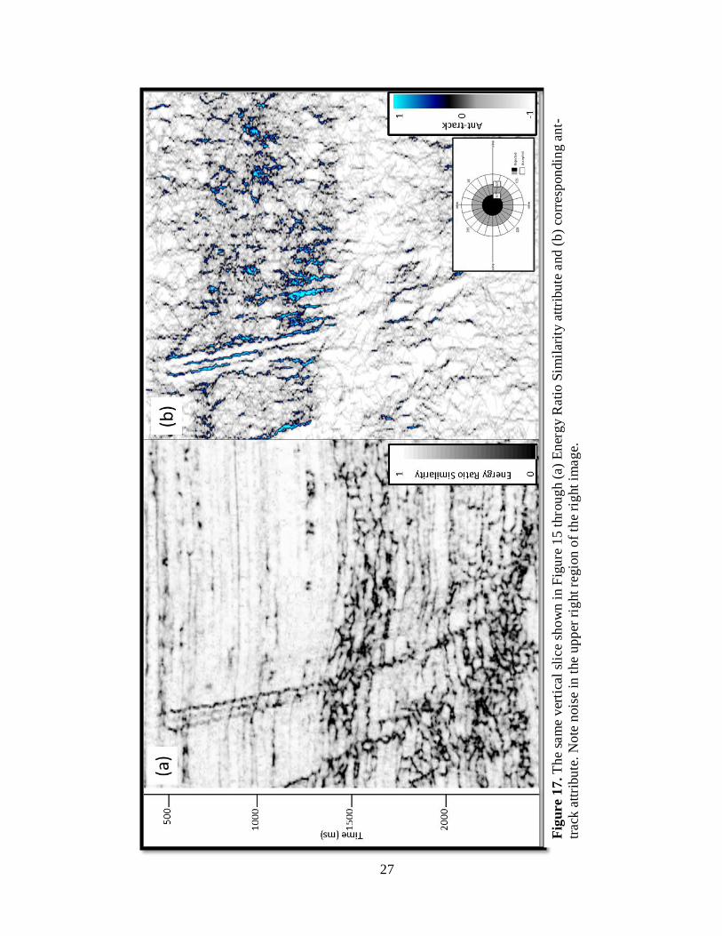
Figure 17. The same vertical slice shown in Figure 15 through (a) Energy Ratio
Similarity attribute and (b) corresponding ant-track attribute. Note noise in the upper
right region of the right image. ........................................................................................... 27
Figure 18. The same vertical slice shown in Figure 15 through (a) first iteration of LoG
attribute and (b) corresponding ant-track attribute. Note noise diminishment in the upper
right region of the right image. ........................................................................................... 28
Figure 19. The same vertical slice shown in Figure 15 through (a) fault probability after
the third iteration of dLoG filtering and (b) corresponding ant-track attribute. Note noise
diminishment in the upper right region of the right image and improved fault resolution.
............................................................................................................................................... 29
Figure 20. Workflow for automatic fault object extraction. ............................................. 33
Figure 21 (a) Seismic cross-section showing three manually picked faults that are
displayed (b) in 3D. Time slice is through the dLoG attribute fault probability. ............ 36
Figure 22. Fault extraction patches (left) for LoG, variance and energy ratio similarity.
The histograms to the right represent the patches sorted by surface area. ....................... 37

x
Figure 23. Histogram showing the similarity of computer-assisted fault extraction to
manually extracted faults shown in Figure 21 for faults generated using (a) LoG and (b)
variance. ............................................................................................................................... 38

xi
Abstract
Fault picking is a critical, but human-intensive component of seismic
interpretation. In a bid to improve fault imaging in seismic data, I have applied a
directional Laplacian of a Gaussian (dLoG) operator to sharpen fault features within a
coherence volume. I compute an M by M matrix of the second moment distance-
weighted coherence tensor values that fall within a 3D spherical analysis window about
each voxel. The eigenvectors of this matrix define the orientation of planar
discontinuities while the corresponding eigenvalues determine whether these
discontinuities are significant. The eigenvectors, which quantify the fault dip-
magnitude and dip-azimuth, define a natural coordinate system for both smoothing and
sharpening the planar discontinuity. By comparing the vector dip of the discontinuity to
the vector dip of the reflectors, I can apply a filter to either suppress or enhance
discontinuities associated with unconformities or low signal-to-noise ratio shale-on-
shale reflectors. Such suppression become useful in the implementation of subsequent
skeletonization algorithms. Automatic fault picking processes for accelerated
interpretation of basins also become much easier to implement and more accurate. I
demonstrate the value and robustness of the technique through application to two 3D
post stack data volumes from offshore New Zealand, which exhibit polygonal faulting,
shale dewatering, and mass-transport complexes. Finally, I use these filtered faults as
input to an ant-tracking algorithm and automatic fault extraction and find significant
improvement in the speed and accuracy of fault interpretation.

1
Chapter 1: Directional Laplacian of a Gaussian theory
The next section is extracted from Machado et al (2016).
Eigenvector estimation of fault dip and azimuth
This work is based on Barnes’ (2006) contribution to edge detection methods,
where he constructed a second moment tensor using an edge attribute, αm, = 1 – cm ,
where cm is coherence, with an M-voxel analysis window
, (1)
where the variables xim and xjm are the distances from the center of the analysis window
along axis i and j of the mth data point respectively. In order to numerically support the
dLoG operator, the analysis window needs to include at least seven traces along the x
and y-axes, thereby defining a sphere of points in x, y and z where the z axis defines
depth converted samples.
In the absence of an anomaly the value of αm in equation 1 will be zero. In a
three-dimensional setting, the second moment tensor C has three eigenvalues, λj, and
eigenvectors, vj. By construction:
. (2)
The values of λ3 and v3 are key to subsequent analysis. If λ1 ≈ λ2 >> λ3, the edge
attribute defines a plane that is normal to the third eigenvector, v3. . If λ1 ≈ λ2 ≈ λ3 then
the coherence data represents either chaotic (λ3 large) or homogeneous (λ3 small) seismic
facies. In such cases, the orientation of the geological feature becomes randomized and
does not represent a planar discontinuity. The eigenvectors v1 and v2 define a plane that
M
m
m
M
m
mjmim
ij
xx
C
1
1
321

2
least-squares fits the cloud of edge attributes, αm. Figure 1 shows a cartoon of the
analysis window used to calculate the attribute enhancement.
In order to display the orientation of a planar feature, I define the “fault” dip
magnitude, θ, to be
)ACOS( 33v , (3)
and the “fault” dip azimuth, to be
, (4)
with the three components of eigenvector v3 defined as
333322311ˆˆˆ vvv xxxv3 (5)
where the x1-axis is oriented positive to the North, the x2-axis positive to the East, and
the x3-axis positive down. Here I use the word “fault” in quotes; while I am interested in
mapping and enhancing faults, this method works similarly for mapping any
discontinuity, such as angular unconformities. If the input attributes αm were most
positive curvature, I would sharpen fold axes. The word “fault” will help me
differentiate these dips from those of the reflector’s dip-magnitude and dip-azimuth that
I will discuss later. Using a multiattribute display technique described by Marfurt
(2015), I plot fault dip-azimuth against a cyclical color bar, fault dip-magnitude against
a monochrome gray scale, and the fault probability against a monochrome white scale
(Figure 2). Note in this image that the fault dip-azimuth ranges between -1800 and
+1800. Thus a near vertical fault dipping towards the southwest may be described by
(θ=800, ψ=-1200) and appears as green, while one dipping to the northeast may be
described by (θ=800, ψ=+600) and appears as magenta. The accuracy of the fault dip
magnitude depends on the accuracy of the time-depth conversion described earlier. This

3
color mapping results in horizontal features such as unconformities appearing as
monochrome gray.
Fault smoothing and edge enhancement using the directional Laplacian of a Gaussian
operator
Laplacian operators are commonly used in sharpening photographic images
(Millan and Valencia, 2005). Unfortunately, such sharpening can exacerbate short
wavelength noise. In contrast, Gaussian operators are used to smooth such images. The
“Laplacian of a Gaussian” or LoG operator avoids some of the artifacts of the Laplacian
operator itself by smoothing high frequency artifacts prior to sharpening. Using the
associative law when creating the operator, one finds that
. (6)
The composite LoG operator will have the general form:
, (7)
where σ2 defines the variance of the Gaussian smoother.
Such a mathematical implementation has two advantages. First, one can
precompute the LoG operator, rather than cascade two separate operations, resulting in
a more efficient algorithm. Second, one is no longer restricted to orienting the Laplacian
operator along the seismic acquisition axes, allowing one to implement a directional
filter.
(LG)αGαL
M
m
mmmmmmm xxxxxx
12
2
3
2
2
2
1
2
2
3
2
2
2
1
4 2exp
31
1
LGα

4
Directional smoothing and sharpening
I modify the dLoG operator to be directional, smoothing along the direction
perpendicular to the planar discontinuity defined by the eigenvectors v1 and v2. I define
the Gaussian to be elongated along the planar axes:
*
+ , (8)
where Σ is defined as:
(
) (9)
And where σ1= σ2= 3σ3, and where x’ indicates the coordinates of the voxels in the
analysis window within the rotated coordinate system, aligned with the hypothesized
fault. In my examples, the bin size Δy = 25m, Δx = 12.5m; to have good numerical
support of the dLoG I set σ3 = 25 m and σ1= σ2= 75 m. In my original (unprimed
system), the Gaussian then becomes:
[ ] , (10)
where R is the rotation matrix that aligns the new x’-axis with v3 given by:
. (11)
The second derivative of the Gaussian in the x3’direction can be written as:
*
+ *
(
)+ , (12)
where γ represents a normalization term.
vvvvvvvvv
332313
322212
312111
R
3
2
3
2
2
2
1
2
12
3
3
2
3
2
exp42
xxxxnorm
dx
Gd
3
2
3
2
2
2
1
2
12
3
3
2
3
2
exp42
xxxxnorm
dx
Gd
3
2
3
2
2
2
1
2
12
3
3
2
3
2
exp42
xxxxnorm
dx
Gd
3
2
3
2
2
2
1
2
12
3
3
2
3
2
exp42
xxxxnorm
dx
Gd
3
2
3
2
2
2
1
2
12
3
3
2
3
2
exp42
xxxxnorm
dx
Gd

5
Figure 1. Cartoon showing reflectors (as solid red lines) and a coherence anomaly (as
black dotted line). The analysis window (in green) is a circle centered on the analysis
point (in orange). The eigenvector v3 is perpendicular to the fault plane reflector (blue
arrow), while the normal vector n is perpendicular to the reflector (red arrow). The
dLoG operator (red negative and blue positive) is short in the direction parallel to v3 and
three times longer in the direction parallel to v1 and v2
6
Fig
ure 2
. T
ime
slic
e at
t=
2.5
2 s
thro
ug
h c
o-r
ender
ed f
ault
dip
-azi
mu
th,
fau
lt d
ip-m
agn
itu
de
and
LoG
fil
tere
d c
oh
eren
ce
(fau
lt p
robab
ilit
y).
The
fau
lt p
robabil
ity
is
plo
tted a
gain
st lig
htn
ess,
wit
h l
ow
val
ues
opaqu
e (w
hit
e) a
nd h
igh v
alu
es
tran
spar
ent.
7
Chapter 2: dLoG application on two New Zealand basins
The next section was also published in Machado et al (2016).
I evaluate my proposed algorithm by applying it to two seismic volumes from
offshore New Zealand. The first survey is over the Great South Basin (GSB) that lies
off the southeast coast of the South Island of New Zealand. The basin formed during the
mid-Cretaceous and is divided into several highly faulted sub-basins. The second
survey is from the Canterbury Basin of the eastern coast of South Island, New Zealand.
A geologic summary is provided in the Appendix.
Great South Basin
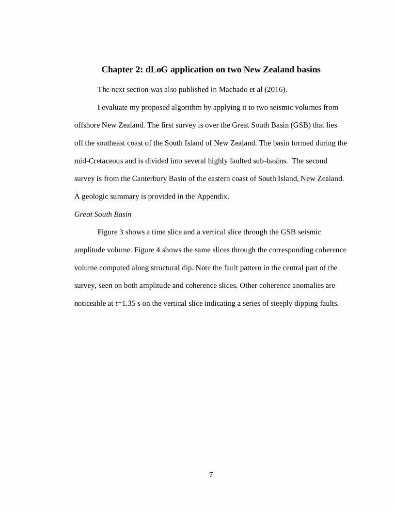
Figure 3 shows a time slice and a vertical slice through the GSB seismic
amplitude volume. Figure 4 shows the same slices through the corresponding coherence
volume computed along structural dip. Note the fault pattern in the central part of the
survey, seen on both amplitude and coherence slices. Other coherence anomalies are
noticeable at t=1.35 s on the vertical slice indicating a series of steeply dipping faults.

8
Figure 3. (a) Time slice at t=2.52 s and (b) vertical slice along AA' through a seismic
amplitude volume with a bin size of 12.5 by 25 m.
9
Figure 4. (a) Time slice at t=2.52 s and (b) vertical slice along AA' through a coherence
volume computed from the seismic amplitude data shown in Figure 3. The orientation
of the coherence anomalies in (a) are shown on Figure 2.

10
I now sharpen the image shown in Figure 4 through the application of the dLoG
operator and display the results in Figure 5. Using a conversion velocity of 3000 m/s
and a 75 m radius analysis window the directional LoG filter sharpens the fault features
and removes high frequency noise from the input coherence volume. In addition to
sharpening, I apply a filter (Figure 5c) that suppresses coherence anomalies parallel to
reflector dip. Fault features indicated by block arrows are more prominent and easier to
pick while some of the noise is suppressed. The conversion velocity was the same as
that used to compute reflector dip and azimuth.
Note that the dLoG filter followed by a dip magnitude filter enhances the faults
at t=1.35 s in the upper portion of the vertical cross-section and improved its continuity.

11
Figure 5. (a) Time slice at t=2.52 s and (b) vertical slice along AA' through the
directional dLoG attribute computed from the coherence volume shown in Figure 5. (c)
Filter applied to coherence computed from the dip magnitude of v3 that suppresses
features parallel to reflector dip. Block blue arrows indicate faults that are now more
continuous and easier to identify.

12
Figure 6 shows the components of eigenvector v3 co-rendered with the
directional dLoG fault probability volume. The fault or unconformity dip–magnitude
with respect to the reflector of any given planar event is defined by v33. I plot this
attribute against saturation in an HLS display. The azimuth, ψ, of steeply dipping planar
events (typically faults) is computed from equation 4, where axis 1 is North. Fault
probability values are plotted against transparency such that high fault probability
events appear to be transparent on an otherwise white background.

13
Figure 6. Time slice at t=2.52 s through co-rendered fault dip-azimuth, fault dip-
magnitude, fault probability and seismic amplitude. The fault dip magnitude and
azimuth are computed from v3. The opacity used for each attribute is displayed on top
of the color bar. Fault dip azimuth is plotted against a cyclical color bar, fault dip
magnitude against a monochrome gray scale, the dLoG attribute against a monochrome
white scale and seismic amplitude against a black and white binary color bar. Fault dip
azimuth and magnitude can be easily characterized through this combination of
attributes. Sharpened events sub parallel to the vertical slices appear smeared (blue and
yellow on the N-S line, red and green on the E-W line).

14
Figure 6 clearly exhibits the orientation of the fault systems present in the data.
The southern faults on the time slice show a predominant southwest dipping direction
(green), while in the northern region I can see an eastward dipping direction. On most
of the faults, I can see a nearly parallel fault of opposite azimuth, representing the
fundamental motion of faults defining horsts and grabens appearing as green/pink
(west/east) and the blue/yellow (north/south) linear couplets. On the vertical slices, the
orientation of the fault azimuth is more clearly seen. Faults sub parallel to the vertical
slice appear “blurred”. Notice the northward-dipping faults in the upper left portion of
the image, with the events clearly shown in the overlaid seismic amplitude.

15
Figure 7. (a) Time slice at t= 2.8 s through co-rendered fault dip-azimuth, fault dip-
magnitude, fault probability and seismic amplitude. The fault dip magnitude and
azimuth are computed from v3. The opacity used for each attribute is displayed on top
of the color bar. Fault dip azimuth is plotted against a cyclical color bar, fault dip
magnitude against monochrome gray the fault probability attribute against monochrome
white and seismic amplitude against a black and white dipole color bar. Shale
dewatering features are pointed with the blue block arrow. (b) and (c) show two vertical
lines with orthogonal orientation and the seismic image of the shale dewatering features
with an outward dipping trend.

16
The dip magnitude of the fault features is also displayed on Figure 6. Notice
how the southern fault system (right side of the image) is less bright than the northern
one, which indicates that it is less vertical. Most of the horizontal events were
suppressed by the application of the filter shown in Figure 5c.
Canterbury Basin
Figure 7 shows a seismic image of shale dewatering features from the
Canterbury Basin survey acquired in New Zealand. The directional Laplacian of a
Gaussian highlights and sharpens the linear features, while the eigenvectors represent
their azimuth and dip magnitude. Examination of the polygonal fault system highlighted
shows an outward-dipping trend for most of the features.
Figure 8 shows seismic images of a turbidity system in the Canterbury Basin
survey before and after directional dLoG filtering of coherence. The coherence image in
Figure 8a shows channels in the central and northeastern portion of the image. Figure
8b after dLoG and dip magnitude filtering shows an image that is noticeably cleaner,
with discontinuities more sharply defined. Finally, Figure 8c shows the steeply dipping
edge channels through the “fault” dip-magnitude and dip-azimuth. Notice how the
northern edge of the channels of the central portion of the image is dipping northward.
This can also provide information on the nature and depositional direction of the
sediments.

17
Figure 8. Time slice at t=2.04 s through a) coherence, b) dLoG of coherence fault
probability c) co-rendered fault dip-azimuth, fault dip-magnitude and dLoG of
coherence (“fault” probability). The fault dip magnitude and azimuth are computed
from v3. The transparency function used for each attribute is displayed on top of the
color bar. Fault dip azimuth is plotted against a cyclical color bar, fault dip magnitude
against a monochrome gray color bar, fault probability against a monochrome white
color bar. Channel features are easily recognized through the conventional coherence,
but sharpened and cleaner after dLoG filtering. The channel edges are further
characterized by combining with fault dip magnitude and azimuth attributes.
18
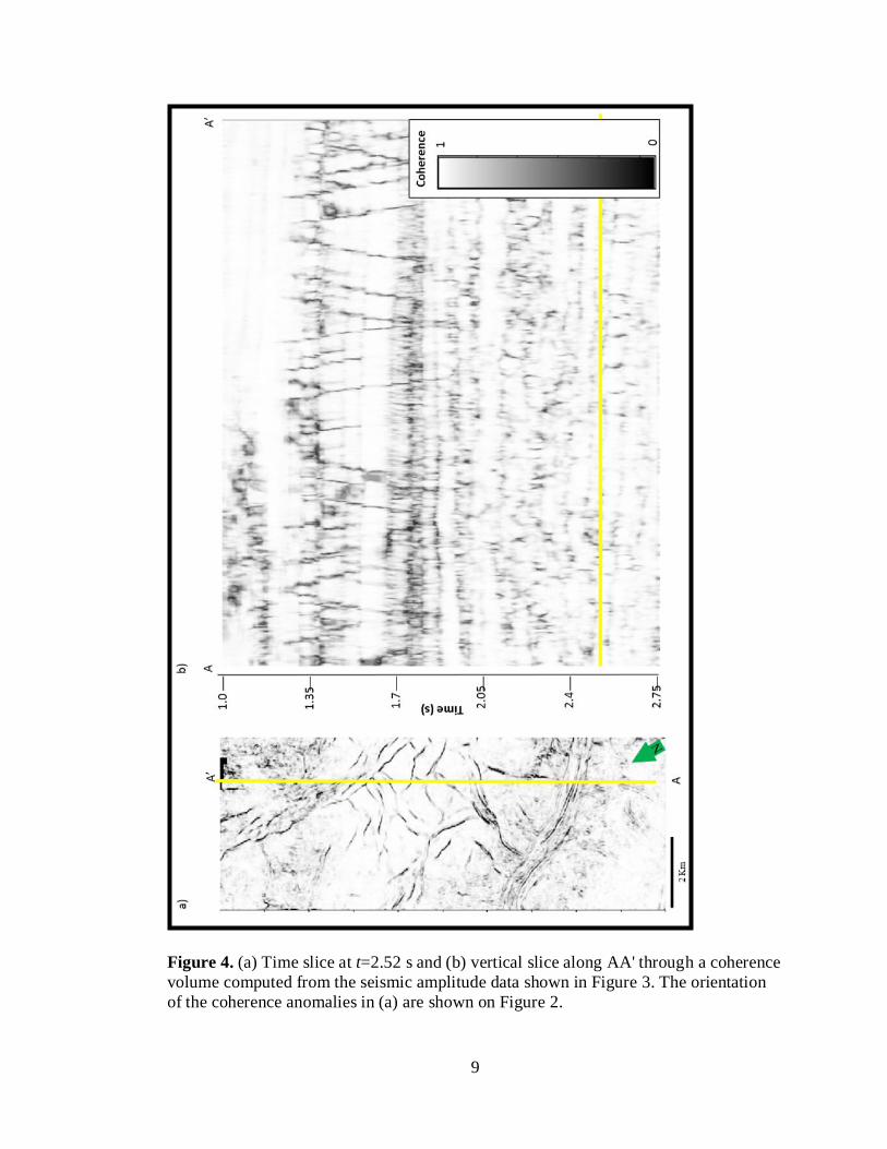
Figures 5-8 showed images generated using the dip magnitude filter described in
Figure 5c. Similar filters can be designed on either dip-azimuth. Figures 9 and 10 show
two different tapers applied to the same dataset at the same depth as the one shown on
Figure 6. In Figure 9, I enhance low coherence events parallel to structural dip, and
reject discontinuities with a dip greater than 25°. Such features appear grayer since the
reflectors are relatively flat.
Figure 9. Time slice at t= 2.52 s through faults shown in Figure 6 highlighting near
horizontal discontinuities through the use of a taper which hinders any feature with a
dip greater than 25°.
In contrast, Figure 10 shows the same slices as in Figure 9 but with a filter that
rejected features with a dip magnitude less than 65°. The faults are brighter since they
are steeper with less of a gray overprint in the display. The faults in the central part of
the survey are more steeply dipping while those to the north have been filtered out.

19
Figure 10. Time slice at t= 2.52 s through faults corresponding to Figure 6 with a dip
magnitude filter that reflects features whose dip is less than 65°.
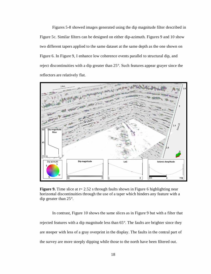
In Figure 11, a box probe was created to isolate and show the 3D image of the
polygonal fault system from the Canterbury Basin dataset. Through co-rendered fault
dip-azimuth and dip-magnitude, with opacity modulated by the dLoG fault probability
attribute, I was able to generate a 3D image of the fault planes. Outward dipping trends
can be seen, especially on the right side of the image.
20
Figure 11. 3D view of two vertical lines through the seismic amplitude volume, and a
box probe through co-rendered fault dip azimuth and fault dip magnitude showing
polygonal faulting. The fault probability modulates the opacity, where vowels with
α<0.5 are being rendered transparent. Lineaments that are less than 25° of dip to the
reflector have been filtered out.
Figure 12 shows the same box probe as Figure 11. By making use of the same
co-rendering parameters I am able to isolate faulting features within a limited range of
azimuth. Such manipulation of the dip azimuth of these features allows me to highlight
antithetic faulting in the basin, as shown by the opposed dipping directions of the faults
portrayed.

21
Figure 12. The same image as Figure 11, but now with faults with N and S azimuths
rendered transparent. Thus a synthetic and antithetic fault system is highlighted

22
Chapter 3: dLoG as a preconditioner for ant-tracking and automatic
fault picking
Fault picking is a human intensive labor involved in every aspect of any oil and
gas exploration and production endeavor. In resource plays faults can be geologic
hazard to avoid, while in conventional plays they may also form traps for potential
hydrocarbons accumulation. Because many surveys have dozens or even hundreds of
faults to be selected and analyzed for interpretation, different approaches have been
proposed to solve this problem. One such approach is the ant-tracking algorithm. I used
a commercial implementation of ant-tracking with and without the dLoG attribute to
evaluate the automatic fault extraction process for a dataset from the New Zealand
Taranaki basin.
The ant-tracking algorithm
Ant tracking is an algorithm inspired by the collective foraging behavior of a
real ant colony in the nature (Zhao et al., 2015). The concept was first introduced by in
the nineties by Colorni et al. (1991) and Dorigo et al. (1997) but only recently has it
been adopted by different software platforms as a mean to guide the automatic fault
extraction process. Figure 13, taken from Dorigo et al. (1997), explains the concept
behind the ant tracking quite well. First ants are randomly sprinkled on a grid point after
which they take one of several allowed pathways. Each ant can proceed a fixed number
of steps. If the ant finds food it can go further. If not, it dies. Each deposits pheromones
as it travels and more ants come that way. In this manner, the shorter paths with more
food will be populated with the most ants

23
Figure 13. A model of how real ants find the shortest path. (a) Ants arrive at a decision
point. (b) Some ants choose the upper path and some the lower path. The choice is
random. (c) Since the ants move at approximately a constant speed, the ants that choose
the lower, shorter, path reach the opposite decision point faster than those that choose
the upper, longer, path. (d) Pheromone accumulates at a higher rate on the shorter path
due to a higher amount of ants crossing it. The number of dashed lines is approximately
proportional to the amount of pheromone deposited by ants (taken from Dorigo et al.,
1997).
This concept of swarm intelligence may be applied to geological problems. The
idea is to distribute a large number of agents (ants) into a volume so that they move
along fault surfaces highlighted by some edge enhancement attribute, such as
coherence. Where there are grid points that do not fulfill the conditions for a fault, such
as a continuous seismic reflector surface, agents will be terminated shortly (Iske et al.,
2005). Figure 14 from Iske et al., (2005) illustrates how the ant-tracking algorithm helps
to delineate fault and discontinuities while rejecting noise.

24
Figure 14. (a) Time slice through a fault attribute (variance) with (b) corresponding ant
tracking results (after Iske et al., 2005).
Figure 15 shows a vertical slice through a seismic amplitude volume acquired
over the Taranaki Basin, New Zealand. Note the relatively flat geology for the first
second of seismic data, followed by an unconformity, which is inferred to be an incised
valley. The next part of the seismic section is highly faulted.

25
Figure 15. Seismic amplitude of survey from the Taranaki Basin. Relatively flat
geology on top of normally faulted sequences below 1500 ms. Block arrow indicates an
unconformity.
Figures 16 through 19 show the same cross section shown on Figure 15 through
three different edge enhancement attributes. Each attribute was used as input to generate
an ant-tracking attribute for subsequent automatic fault extraction.

26
Fig
ure 1
6. T
he
sam
e v
erti
cal
sect
ion
fro
m F
igu
re 1
5 t
hro
ugh
(a)
var
ian
ce a
ttri
bu
te a
nd
(b)
corr
esp
on
din
g a
nt-
trac
ked
att
ribu
te.
The
ster
eon
et s
ho
ws
that
ants
wer
e co
nst
rain
ed t
o s
earc
h w
ithin
a c
on
e o
f 3
0°
abou
t th
e v
erti
cal
(fau
lt d
ips
> 6
0°)
.
27
Fig
ure 1
7. T
he
sam
e v
erti
cal
slic
e sh
ow
n i
n F
igu
re 1
5 t
hro
ug
h (
a) E
ner
gy R
atio
Sim
ilar
ity a
ttri
bu
te a
nd
(b
) co
rres
pon
din
g a
nt-
trac
k a
ttri
bu
te.
No
te n
ois
e in
the
up
per
rig
ht
regio
n o
f th
e ri
ght
imag
e.

28
Fig
ure 1
8. T
he
sam
e v
erti
cal
slic
e sh
ow
n i
n F
igu
re 1
5 t
hro
ug
h (
a) f
irst
ite
rati
on o
f L
oG
att
ribu
te a
nd (
b)
corr
espo
ndin
g a
nt-
trac
k
attr
ibu
te.
No
te n
ois
e dim
inis
hm
ent
in t
he
upp
er r
igh
t re
gio
n o
f th
e ri
gh
t im
age.

29
Fig
ure 1
9. T
he
sam
e v
erti
cal
slic
e sh
ow
n i
n F
igu
re 1
5 t
hro
ug
h (
a)
fau
lt p
rob
abil
ity a
fter
th
e th
ird
iter
atio
n o
f d
LoG
fil
teri
ng a
nd
(b)
corr
esp
ond
ing a
nt-
track
att
ribu
te.
No
te n
ois
e dim
inis
hm
ent
in t
he
upp
er r
ight
regio
n o
f th
e ri
gh
t im
ag
e an
d i
mpro
ved
fau
lt
reso
luti
on
.

30
The variance on Figure 16 does a good job in highlighting discontinuities but is
relatively unfocused, which results in a more diffuse ant-track image. Energy ratio
similarity (Figure 17) is a measurement of coherence that works very well with
highlighting and sharpening discontinuities as faults, but also highlights other types of
discontinuities which also affects the corresponding ant-track image. The subtle vertical
discontinuities in the upper right portion of the ant-track algorithm will represent a
challenge for the later automatic fault extraction.
Figure 18 shows the same vertical slice through the directional Laplacian of a
Gaussian fault probability attribute computed iteratively. In the first iteration, I enhance
steeply dipping features but suppress features parallel to reflector dip. With these
stratigraphic features removed, the second iteration of fault enhancement is better able
to link up faults that were previously cut by unconformities and other stratigraphic
discontinuities. The third iteration (Figure 19a) reduces noise such that the resulting
image looks cleaner and sharper. Furthermore, subsequent ant-tracking (Figure 19b)
shows significantly less noise in the upper right portion of the image, which will make
the fault extraction process much simpler.
For each one of the ant-tracked attributes shown on Figures 16-19, the
parameters were as following:

31
Table 1 Ant-tracking parameters for edge enhancement attributes
Ant-tracking Parameter Value
Number of ants 7
Ant track deviation 2
Ant step size 3
Illegal steps allowed 1
Legal steps required 3
Stop criteria 5
The number of ants refers to the ant density the program will be allowed for
fault tracking. A higher value means higher density, but also higher computational time.
Ant track deviation refers to the amount of illegal steps allowed outside of a delimited
fault. The higher this value the more interconnected features will appear in the final
result. The ant step size refers to how many voxels or ants per step are allowed, which
translates into higher resolution for smaller sizes. Illegal steps allowed are the amount
of steps that the algorithm will take outside of a delimited discontinuity. Legal steps
required refers to how connected the faults must be in order distinguish edges from
noise. The stop criteria value is the percentage of illegal steps allowed before
terminating an agents life.

32
Fault object extraction
With the computed attributes I next evaluate how the different images affect a
commercial automatic fault extraction tool. To validate the process, I manually picked
three faults from the seismic data, thus generating my control groups. With considerable
self-confidence, I assume manually picked faults are the closest approximation to
reality. Figure 21 shows a 3D image of the manually picked faults, along a
representative amplitude slice from which they were taken. All three faults are
prominent in the seismic survey, so they did not represent a big challenge to pick
The workflow for the commercial automatic fault object extraction software
requires an edge enhancement attribute as input. The extraction program generates an
array of fault patches that follows the discontinuities. These patches may be manually
selected and merged to shape the different faults within the survey. Distributions of the
fault patches are generated in the form of histograms which serves to filter them by
surface area, dip azimuth, dip magnitude and height, among others.
A general workflow for the automatic fault extraction is displayed on Figure 20.
First, from an amplitude volume, I compute coherence or other edge enhancement
attribute. Then, through the use of the directional Laplacian of a Gaussian, I enhance
vertical and suppress horizontal features, which will be skeletonized in a subsequent
step with an ant-tracking algorithm. The resulting fault patches are sorted by surface
area, dip azimuth and dip magnitude. For this example I focused on surface area as the
decisive parameter to filter patches. If the patches are too small, they will be rejected.
Otherwise, I will merge them to recreate the manually picked faults

33
Fig
ure 2
0. W
ork
flo
w f
or
auto
mat
ic f
ault
obje
ct e
xtr
act
ion
.

34
Using ant tracking for the attributes shown on Figures 16-19, fault patches were
created and merged to recreate the faults that had already been manually picked. Figure
21 shows a visual and quantitative comparison of the fault patches generated. The
histogram generated for each fault extraction process shows how the different
algorithms affect its accuracy and effectiveness. The less the user needs to interact with
the program, the more effective the workflow becomes in accelerating the fault
definition process
Examining Figure 22a the dLoG input generates the least amount of patches.
The dLoG patches are larger and more continuous, making the future merging process
easier. In the case of variance, the image is fairly good, but gives rise to more small
fault patches and lacks the continuity of dLoG, which results in a more difficult fault
extraction. Finally, the energy ratio similarity is the attribute that yields the worst
results, since its sensitivity to stratigraphic anomalies results in some horizontal
artifacts, such that the manual merging step in the extraction process becomes much
more difficult.
Analyzing the histograms on Figure 22 of the dLoG attribute note the percentage
of small fault patches (<1000 m2) is significantly smaller (about 30% of the patches)
than for the energy ratio similarity. Likewise, the percentage of big fault patches (>5000
m2) is significantly higher for the dLoG computation.
In a bid to quantify the effectiveness and advantages of each attribute for the
fault extraction process, I created a surface out of each fault: first the manually picked
and then the automatically extracted. Afterward, I subtracted the surface generated for
each attribute from the one generated from the manually picked faults. Assuming that

35
the manually picked faults are closer to reality, the closer the subtraction approaches
zero, the more accurate the automatic extraction was, thereby quantifying the attribute
computation. The difference between the automatic fault extraction and the manually
picked one has a significantly higher percentage of zeroes than the computed using the
variance attribute. I did not consider the energy ratio similarity attribute for this
comparison since it did not allow for a proper patch merging process.

36
Fig
ure 2
1 (
a)
Sei
smic
cro
ss-s
ecti
on s
ho
win
g t
hre
e m
anu
ally
pic
ked
fau
lts
that
are
dis
pla
yed
(b)
in 3
D. T
ime
slic
e is
thro
ug
h t
he
dL
oG
att
ribu
te f
ault
pro
bab
ilit
y.

37
Figure 22. Fault extraction patches (left) for LoG, variance and energy ratio similarity.
The histograms to the right represent the patches sorted by surface area.

38
Fig
ure 2
3. H
isto
gra
m s
ho
win
g t
he
sim
ilar
ity o
f co
mpu
ter-
ass
iste
d f
ault
extr
acti
on
to m
anu
ally
extr
act
ed f
ault
s sh
ow
n i
n F
igu
re 2
1
for
fau
lts
gen
erat
ed u
sin
g (
a) L
oG
an
d (
b)
var
iance
.

39
Chapter 4: Conclusions
Fault image enhancement remains a pivotal objective in seismic data
interpretation. Eigenvector analysis provides a means of volumetrically comparing the
dip-magnitude and dip-azimuth of linear discontinuities. The directional Laplacian of a
Gaussian sharpens fault images and improves fault continuity seen on the input
coherence volume.
I thus have measures not only of strength of discontinuities but also of their
orientation. Using such measures, I can reject or enhance geologic features and noise
aligned with reflector dip, or generate image of faults that fall within an interpreter-
defined azimuthal orientation. Such quantification of the orientation may facilitate
statistical correlation of production to a given fault set or provide the anisotropic
variogram used in geostatistical analysis of turbidite and fluvial deltaic deposits.
Application of the same algorithm to curvature anomalies provides measures of dip and
azimuth of axial planes.
Automatic fault extraction processes benefit from the application of this attribute
enhancement. Not only do fault patches become more continuous and recognizable for
merging and interpretation, noise removal improves the speed at which such
computations may be performed. The accuracy of the process also becomes improved,
as the automatically extracted faults closely resemble the reality represented by the
manually picked faults.

40
References
Aare, V., and B. Wallet, 2011, A robust and compute-efficient variant of the Radon
transform: GCSSEPM 31st Annual Bob. F. Perkins Research Conference on Seismic
attributes – New views on seismic imaging: Their use in exploration and production,
550-586.
Barnes, A. E., 2006, A filter to improve seismic discontinuity data for fault
interpretation: Geophysics, 71, P1-P4.
Colorni, A., M. Dorigo, and V. Maniezzo, 1991, Distributed optimization by ant
colonies: Proceedings of European Conference on Artificial Life, 134–142.
Dorigo, M., and L. M. Gambardella, 1997, Ant colony system: a cooperative learning
approach to the traveling salesman problem: IEEE Transactions on Evolutionary
Computation, 1, no. 1, 53– 66.
Great South-Canterbury Province. (2015, December 07). Retrieved May 07, 2016, from
http://www.nzpam.govt.nz/cms/tools-and-servives/geoscience-exploration-data.
Iske, A., and Randen, T. (2005). Mathematical methods and modelling in hydrocarbon
exploration and production. Berlin: Springer.
Machado, G., A. Abdulmohsen, B. Hutchinson, O. Oluwatobi, and K. Marfurt, 2016.
Display and enhancement of volumetric fault images. Interpretation V 4, No. 1, pp,
SB51- SB61
Marfurt. K, 2015, Techniques and best practices in multiattribute display: Interpretation,
1, B1-B23.
41
Marfurt, K. J., 2006: Robust estimates of reflector dip and azimuth: Geophysics, 71,
P29-P40.
Millán M. S., and E. Valencia, 2006, Color image sharpening inspired by human vision
models: Applied Optics, 45, Issue 29, 7684-7697 doi.org/10.1364/AO.45.007684
Russell, B.H., 1989, Statics corrections – a tutorial: Canadian Geophysical Society,
http://74.3.176.63/publications/recorder/1989/03mar/mar1989-statics-corrections.pdf.,
accessed 12 April, 2016.
Zhao, Y., Yue Y., Huang J., Yu Q., Liu Bingqing., and C. Liu 2015, Study and
application of three parameters wavelet multi-scale ant tracking technology. SEG
Technical Program Expanded Abstracts 2015: pp. 1866-1870.

42
Appendix: Geologic Background of the Great South Basin
The Great South Basin (GSB) is one of the largest basins of New Zealand, with
a surface area of approximately 200000 km2. The basin is a complex intracontinental of
Cretaceous age failed rifts, evolving into subsiding basins during the Late Cretaceous
and Paleocene. Figure A1 shows the areal extent of the Great South Basin, along with
the Canterbury Basin to the north. The thickness approaches 6 km, which equals almost
20000 ft.
The basin has horst and grabens architecture, with plays that have been explored
since the late 1960s including stratigraphic drape over basement highs, faulted
anticlines, folds, turbidity channels, and basin floor fans, among others. Figure A2
shows a vertical cross section of the Great South Basin colored by the age of the
sediments. All petroleum system elements are present in the basin (Figure A3).

43
Figure A1 Location of Great South Basin. Thicknesses in the basin range from 0-6 km
(from a New Zealand Petroleum and Mineral report, 2015).

44
Figure A2. Vertical cross section of the Great South Basin with sediments colored by
age of deposition (from a New Zealand Petroleum and Mineral report, 2015).
Figure A3. Petroleum system elements from the Great South Basin (from a New
Zealand Petroleum and Mineral report, 2015).