University of Hawaii Active Learning with Support Vector Machines By: Estefan Ortiz

University of Hawaii

Active Learning with Support Vector Machines

By: Estefan Ortiz


Outline

Introduction Machine Learning Motivation for the need of Active Learning Active and Passive learners Formulation of Active learning

Support Vector Machines Review of SVMs Version Space Reformulation of SVMs in Version Space

Active Learning using SVMs Formulation of Active Learning using SVMs Querying Algorithms

Implementation of Active Learning using SVMs Data sets used Results Observations and lessons learned Future research and suggested improvements

Conclusion


Machine Learning

Machine learning The purpose of any type of machine learning is to be able teach a learner an

underlying process from observed examples or data. Supervised training

We are given training examples and their corresponding labels. Our task is to teach the machine to recognize the correspondence between the

data and the labels. For classification this amounts to learning the classes associated to underlying

data. In training we present the learner with a feature vector and its corresponding

label and ask it to adjust itself to learn the relationship.


Supervised Learning

What is assumed for this type of learning is that we have gathered a significant amount of data. (Feature vectors and their labels)

The data gathered is usually randomly sampled from some underlying probability distribution.

For each sample in our data set we are able to assign it a label. Consider two situations:

Situation 1: We have limited resources for feature data and to gather large amounts of random samples may be too expensive.

Situation 2: We have access to a large quantity of unlabeled feature data. But to label the data will cost us something. Usually time or money


Motivation for Active Learning

Situation 1: Limited resources This situation may come from a machine process in which it is too costly to

halt the process to take large samples or measurements. In this case we would like a method to choose the “best” set of samples such

that when we train our learner will have a good set of training data. Situation 2: Large amount of unlabeled data

This situation occurs in article classification to some topic. There is a large database of articles, the task is for someone to read through and

assign to each article a topic. The cost is time and money to assign a topic to every article. We would like to choose the “best” set of examples to be labeled so that our

cost is low and our training set is good for our learner. In both situations it would be beneficial to devise a way to choose the

“best” examples for our training set.


Active and Passive Learners

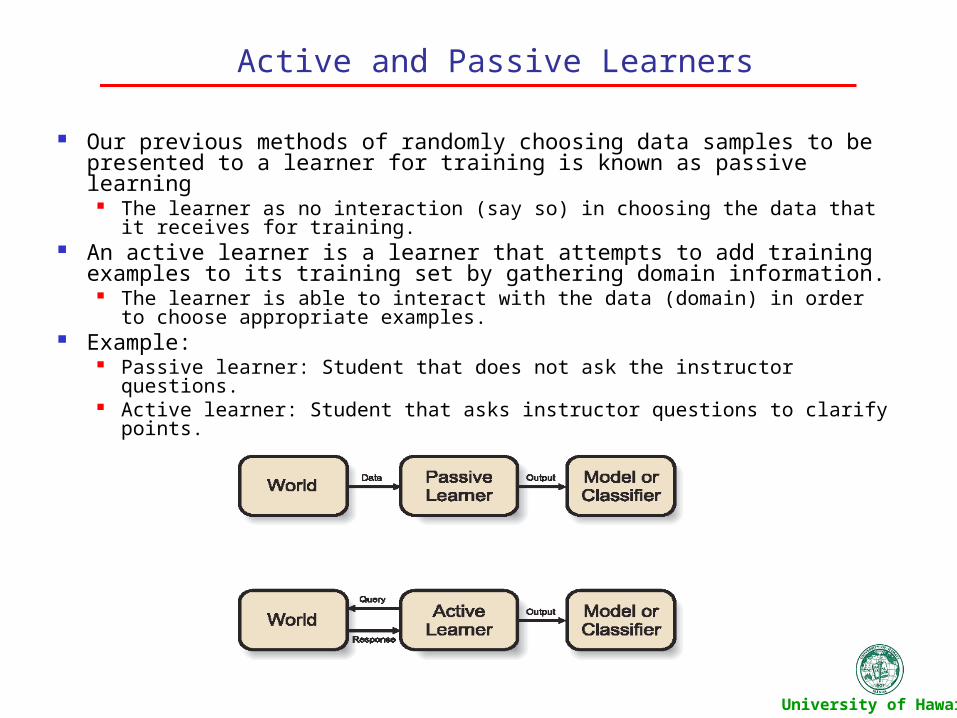
Our previous methods of randomly choosing data samples to be presented to a learner for training is known as passive learning

The learner as no interaction (say so) in choosing the data that it receives for training.

An active learner is a learner that attempts to add training examples to its training set by gathering domain information.

The learner is able to interact with the data (domain) in order to choose appropriate examples.

Example: Passive learner: Student that does not ask the instructor questions. Active learner: Student that asks instructor questions to clarify points.


Active Learning: A Formal Definition

Definition: Active Learning (Schon and Cohn) Active learning is the closed loop phenomenon of a learner selecting

actions or making queries that influence what data are added to its training set.

This formulation has its origins in pool based learning Given pool of unlabeled data we are only allowed to choose n samples

to be labeled for training. Pool based learning also arises from situations in which unlabeled data

is easily available.

The main concept involved in active learning is finding ways to obtain good requests (queries) from the data pool.


Active Learning: Formulation

Define the following concepts needed for active learning Notion of a Model and its associated Model Loss A querying component q such that it will illicit response r from the domain or

data. A type of learner.

The Model will have the following properties: It has some intrinsic loss (Model Loss) due to the lack of knowledge of the

domain space. We are afforded the ability to reduce this loss by making queries q to the data

and using the received responses r.


Active Learning using Support Vector Machines

Outline of application of active learning with support vector machines Review notions of support vector machines as they apply to active learning

SVMs as a binary classifier Feature Space via kernel methods Form of the set of classifiers in feature space

Version Space Assumptions for version space Version Space a Visual Example Reformulation of SVMs in Version space

Model and Model Loss formulated for SVMs Version Space as the model Justification

Querying Algorithm Simple Margin


Review of Support Vector Machines

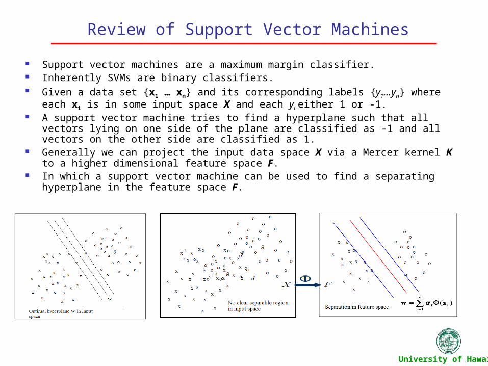
Support vector machines are a maximum margin classifier. Inherently SVMs are binary classifiers. Given a data set {x1 … xn} and its corresponding labels {y1…yn} where each xi is in some input

space X and each yi either 1 or -1. A support vector machine tries to find a hyperplane such that all vectors lying on one side of the

plane are classified as -1 and all vectors on the other side are classified as 1. Generally we can project the input data space X via a Mercer kernel K to a higher dimensional

feature space F. In which a support vector machine can be used to find a separating hyperplane in the feature

space F.


Review of Support Vector Machines

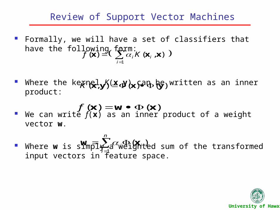
Formally, we will have a set of classifiers that have the following form:

Where the kernel K(x,y) can be written as an inner product:

We can write f(x) as an inner product of a weight vector w.

Where w is simply a weighted sum of the transformed input vectors in feature space.

n

iii Kf

1

),()( xxx

)()(),( yxyx K

)()( xwx f

n

iii

1

)(xw


Version Space

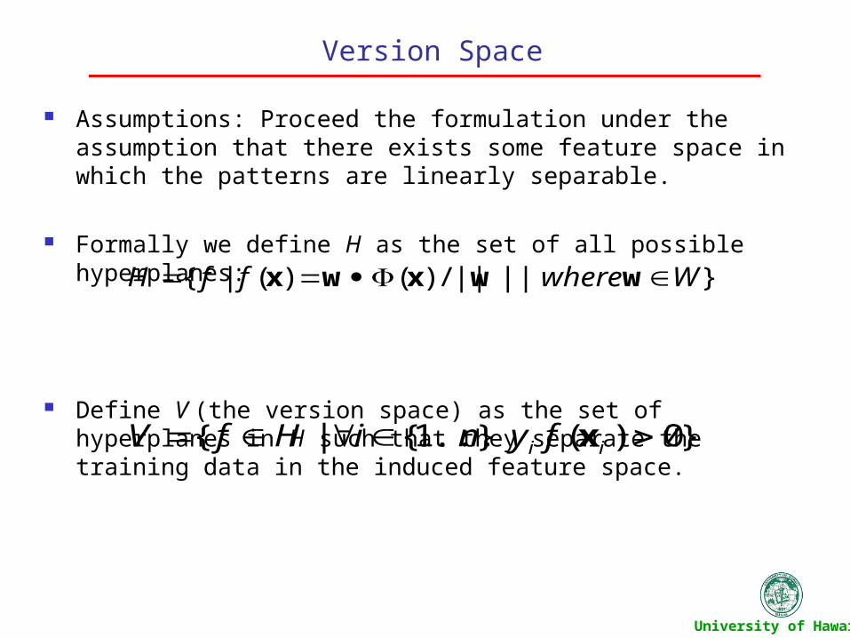
Assumptions: Proceed the formulation under the assumption that there exists some feature space in which the patterns are linearly separable.

Formally we define H as the set of all possible hyperplanes:

Define V (the version space) as the set of hyperplanes in H such that they separate the training data in the induced feature space.

}||||/)()(|{ WwhereffH wwxwx

}0)(}...1{|{ ii fyniHfV x


Version Space: Visual Example

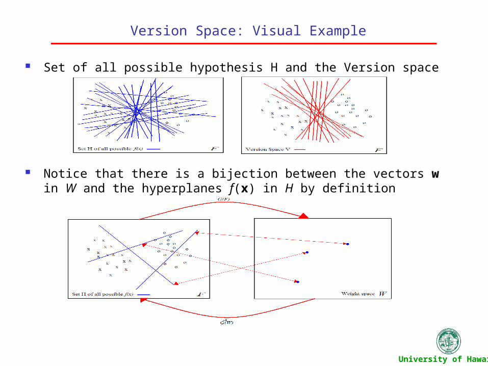
Set of all possible hypothesis H and the Version space

Notice that there is a bijection between the vectors w in W and the hyperplanes f(x) in H by definition


Version Space contd.

Since there is a bijection between H and W we can redefine the version space as.

Suppose, we observe a single input vector xi in feature space (and its corresponding label) and we wish to classify it via some hyperplane.

By doing so we limit the set of hyperplanes to those that will classify xi correctly.

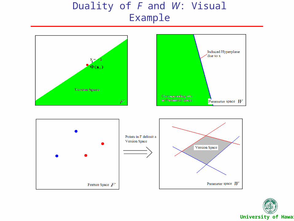
In the parameter space W this has the effect of restricting points in W (w’s) to lie on one side of a hyperplane or the other in W.

This leads to the duality between the feature space F and parameter space W. Formally stated points in F correspond to hyperplanes in W.

}1,0))((,1|||||{ niyWV ii xwww


Duality of F and W: Visual Example


Reformulation of SVMs in Version Space

We know that SVMs find the hyperplane that maximizes the margin in feature space F.

This problem can be reformulated such that:

This formulation is finding w in the version space such that it maximizes the minimum distance to any of the delimiting hyperplanes.

A SVM will find the w such that: w is the center of the largest hypersphere. In which this hypersphere can be placed in the version space without intersecting

the delimiting hyperplanes formed from the labeled training data.

niyandytosubjectMaximize iiiiiF :10))((,1||||))},(({min{ xwwxww


Active Learning using SVMs

An active learner has three main components (f,q,X) f is the classifier X is a set of labeled training data q is the query function that is able to query an unlabeled data set U

Define the model in this setting as version space V. Define the model loss as the size of the version space. Want to query the unlabeled data pool U such that we decrease the model

loss. Finding the best query q so that the response r will return a data point

which reduces the size of the version space Define the size or area of a version space as the surface area that

surrounds the hypersphere ||w|| =1. Denote it as Area(V).


Justification of Version Space as a Model

If we had all the possible training data we could find the optimal w* which will exist somewhere in the parameter space W.

We know that w* will lie in each of the version spaces created by each of the queries to the unlabeled data set U.

Decreasing the version space will in turn reduce the area which w* can exist.

Which in turn gives a w that is closer to the optimal w*.


Querying function

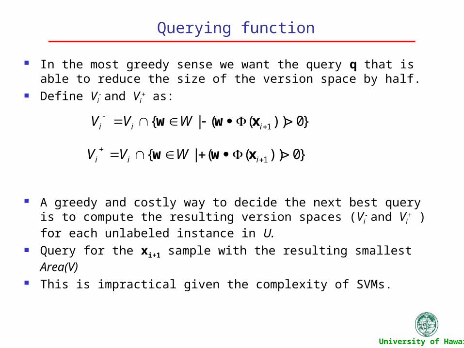
In the most greedy sense we want the query q that is able to reduce the size of the version space by half.

Define Vi- and Vi

+ as:

A greedy and costly way to decide the next best query is to compute the resulting version spaces (Vi

- and Vi+ ) for each unlabeled instance in U.

Query for the xi+1 sample with the resulting smallest Area(V) This is impractical given the complexity of SVMs.

}0))((|{ 1

iii WVV xww

}0))((|{ 1

iii WVV xww


Querying Algorithm

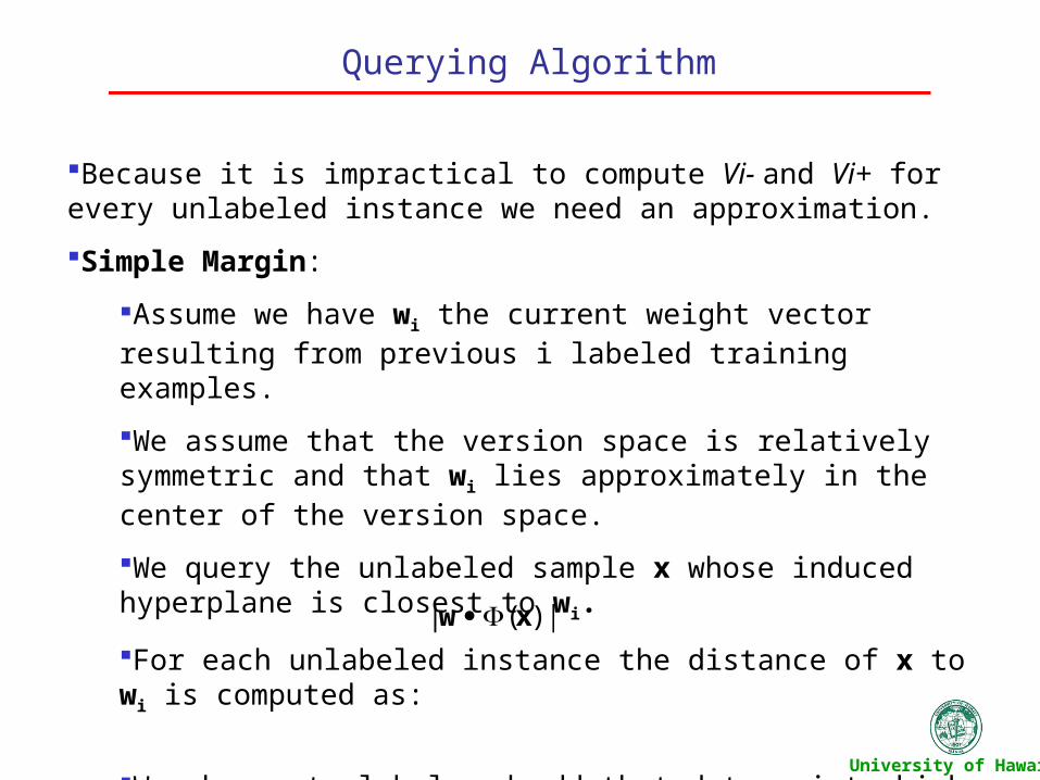
Because it is impractical to compute Vi- and Vi+ for every unlabeled instance we need an approximation.

Simple Margin:

Assume we have wi the current weight vector resulting from previous i labeled training examples.

We assume that the version space is relatively symmetric and that wi lies approximately in the center of the version space.

We query the unlabeled sample x whose induced hyperplane is closest to wi.

For each unlabeled instance the distance of x to wi is computed as:

We choose to label and add that data point which is closest to wi.

|)(| xw


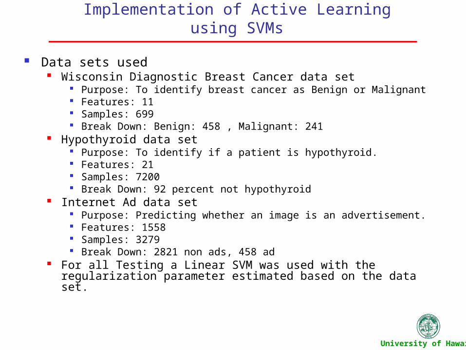
Implementation of Active Learning using SVMs

Data sets used Wisconsin Diagnostic Breast Cancer data set

Purpose: To identify breast cancer as Benign or Malignant Features: 11 Samples: 699 Break Down: Benign: 458 , Malignant: 241

Hypothyroid data set Purpose: To identify if a patient is hypothyroid. Features: 21 Samples: 7200 Break Down: 92 percent not hypothyroid

Internet Ad data set Purpose: Predicting whether an image is an advertisement. Features: 1558 Samples: 3279 Break Down: 2821 non ads, 458 ad

For all Testing a Linear SVM was used with the regularization parameter estimated based on the data set.


Wisconsin Breast Caner Data

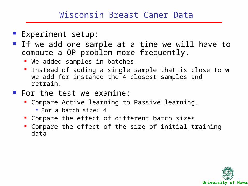
Experiment setup: If we add one sample at a time we will have to compute a QP

problem more frequently. We added samples in batches. Instead of adding a single sample that is close to w we add for instance

the 4 closest samples and retrain. For the test we examine:

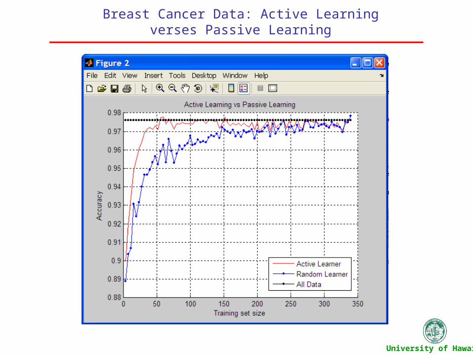
Compare Active learning to Passive learning. For a batch size: 4

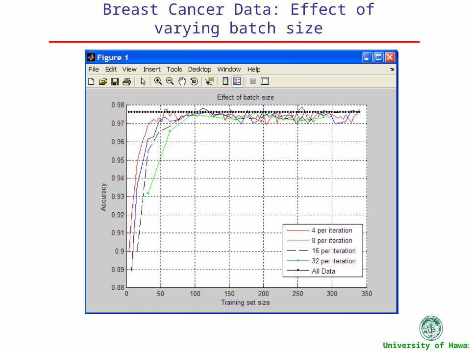
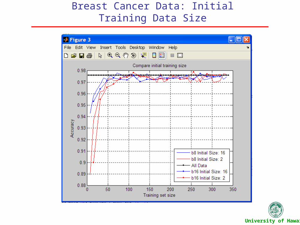
Compare the effect of different batch sizes Compare the effect of the size of initial training data


Breast Cancer Data: Active Learning verses Passive Learning


Breast Cancer Data: Effect of varying batch size


Breast Cancer Data: Initial Training Data Size


Hypothyroid Data Set

For the test we examine: Compare Active learning to Passive learning.

For a batch size: 8 Compare the effect of different batch sizes Compare the effect of the size of initial training data


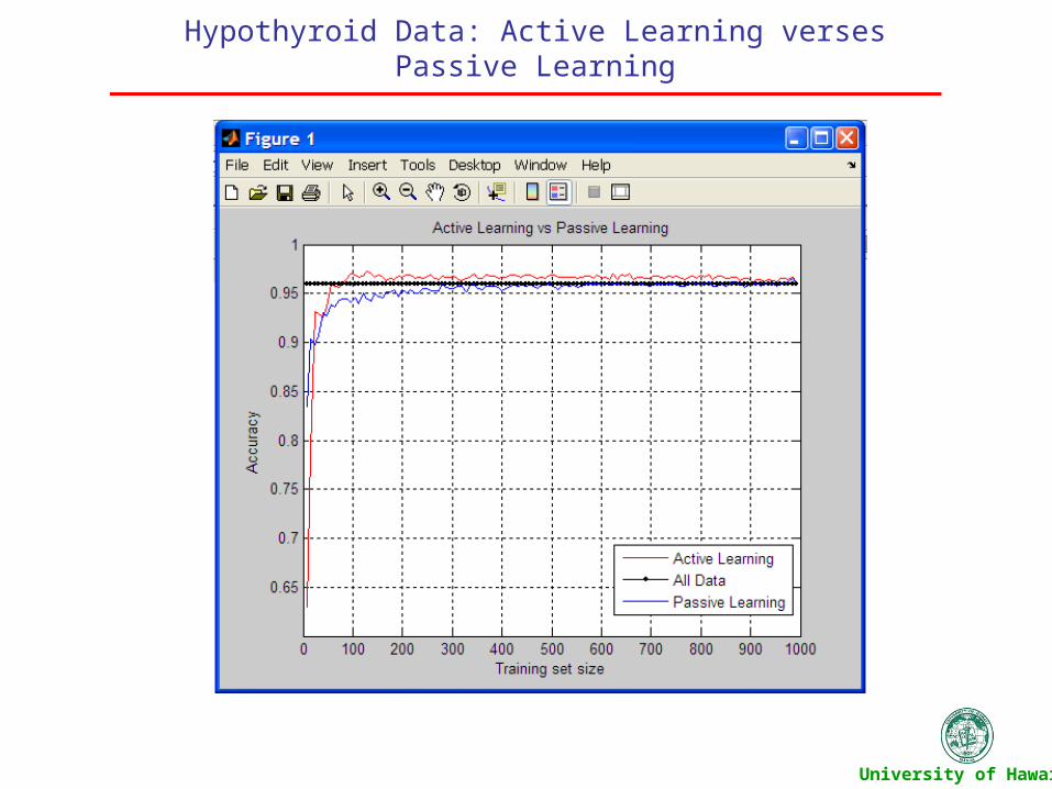
Hypothyroid Data: Active Learning verses Passive Learning


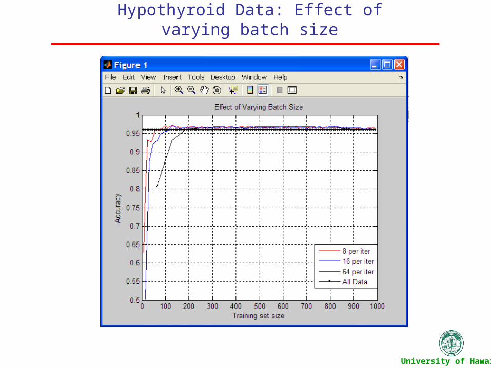
Hypothyroid Data: Effect of varying batch size


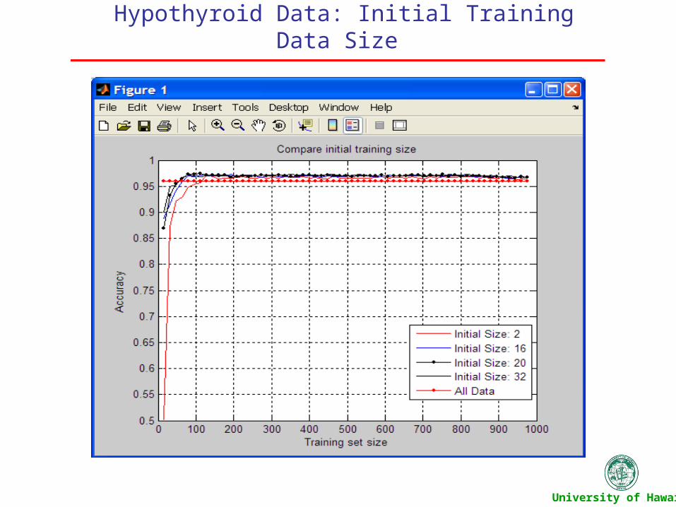
Hypothyroid Data: Initial Training Data Size


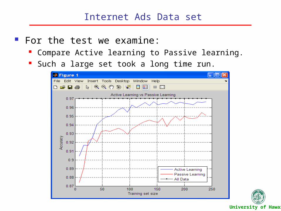
Internet Ads Data set

For the test we examine: Compare Active learning to Passive learning. Such a large set took a long time run.


Conclusions and Future Research

The test results reaffirmed our notion that active learning would perform better than that of a passive learner.

Achieved good generalization . This was able to be accomplished with a smaller data set.

Active learning is a viable technique to use in practice. From our results we can see that the initial number of samples

does effect the performance of active learning. Determine a method to make active learning less dependent on

the size of the initial set of labeled parameters.

Documents

University of Hawaii Active Learning with Support Vector Machines By: Estefan Ortiz