University of Groningen

Strategic interactions in environmental economicsHeijnen, Pim

IMPORTANT NOTE: You are advised to consult the publisher's version (publisher's PDF) if you wish to cite fromit. Please check the document version below.

Document VersionPublisher's PDF, also known as Version of record

Publication date:2007

Link to publication in University of Groningen/UMCG research database

Citation for published version (APA):Heijnen, P. (2007). Strategic interactions in environmental economics s.n.

CopyrightOther than for strictly personal use, it is not permitted to download or to forward/distribute the text or part of it without the consent of theauthor(s) and/or copyright holder(s), unless the work is under an open content license (like Creative Commons).

Take-down policyIf you believe that this document breaches copyright please contact us providing details, and we will remove access to the work immediatelyand investigate your claim.

Downloaded from the University of Groningen/UMCG research database (Pure): http://www.rug.nl/research/portal. For technical reasons thenumber of authors shown on this cover page is limited to 10 maximum.

Download date: 06-05-2018

Chapter 4

Modeling strategic responsesto car and fuel taxation∗

4.1 Introduction

Cars and fuels used for their propulsion are among the most heavily taxed

consumer goods in many countries. In the Netherlands, for example, 42 per-

cent of the consumer price of a new car and 71 percent of the consumer price

of gas are taxes. As a result 13 percent of tax revenues accrues from car use

and ownership. Similar figures are observed throughout the European Union.

The large stakes at hand and the central role of car ownership and use in

daily life make that car and fuel taxation is a subject of continuous public

debate and lobbying.

In the economics literature four types of contributions can be identified

that are relevant for analyzing car and fuel taxation. The first type of contri-

butions are studies that estimate the price elasticity of kilometrage, a para-

meter which is crucial in projecting consumers’ responses to tax changes. This

literature shows a wide range of estimates and suggests that the elasticity is

generally small but non-negligible; see e.g. Goodwin (1992) and Greene, Kahn

and Gibson (1999). The second type of contributions is applied research that

focuses on the environmental impact of car use and various types of fuel; see

for example Crawford and Smith(1995) and Michealis (1995).1 Typically, this

*This Chapter is a version of Heijnen and Kooreman (2006).1Most EU countries have implemented a differential tax treatment (DTT) favoring the

use of diesel. A notable exception is the United Kingdom that – apart from a slightly higher

excise on diesel fuel, treats diesel and gasoline cars equally. The general conclusion fromthe literature is that there is no unambiguous net difference between diesel and gasoline interms of the various emissions, taking into account differences in engine and fuel efficiency.

62 Modeling strategic responses to car and fuel taxation

literature focuses on ‘first-order’ effects, and ignores any possible behavioral

effects in response to changes in the tax regime.

A third type of contributions addresses the question of optimal vehicle

and fuel taxation. In the case of car taxation, it is prohibitively costly (as

yet) to monitor how much of each pollutant each car produces. Several arti-

cles (most notably Fullerton and West, 2002) have investigated second-best

taxes in which different types of cars and different types of fuels can be taxed

differently. Fullerton and West conclude, that even though the number of

instruments is much smaller than the number of pollutants, welfare in the

second-best case can come close to first-best welfare. de Borger (2001) exam-

ines a similar question, but with more emphasis on the decision to buy a car.

The government is restricted to a lump-sum tax on car-ownership and excise

on fuel. Due to the fact that pollution is directly related to the number of

kilometers driven, the optimal taxes are essentially Pigovian. Calthrop and

Proost (2003) provide a good summary of the optimal taxation of cars. In

these kind of studies, neither the car market nor the fuel market are allowed

to be imperfect.

A fourth type of contributions – more recent and small in number – con-

siders potential responses to taxation from an industrial organization per-

spective. The most notable paper in this respect is Verboven (2002), who

provides strong empirical evidence that car manufacturers take advantage of

the favorable differential tax treatment (DTT) for diesel fuel by increasing

the mark-up for diesel cars. More specifically, he finds that 75 to 90 percent

of the price differential between gasoline and diesel cars can be explained by

mark-up differences. Clearly, such responses might well mitigate the intended

effect of the policy.

While Verboven’s analysis is an important step towards a more complete

analysis of the taxation effects, additional steps are necessary. First, Ver-

boven assumes that the price elasticity of demand for kilometrage is exactly

zero. While the empirical literature has generated small price elasticities for

kilometrage demand on average, the assumption of completely inelastic de-

mand is unattractive in any analysis on taxation. Even when elasticities are

small, behavioral effects can be substantial when taxes are high (note that in

many countries taxes almost double consumer prices).2 Secondly, it is likely

DTT might serve as an implicit subsidy on freight transportation in an attempt to boost acountry’s competitiveness. Such a policy, however, is known to be inefficient from a supra-national point of view.

2In theory, moreover, a zero price elasticity of kilometrage would allow fuel producers

Chapter 4 63

that DTT also affects the pricing behavior of fuel companies, an aspect not

analyzed in Verboven.

The purpose of this Chapter is to set further steps to a coherent eco-

nomic analysis of car and fuel taxation by developing a model that describes

the interactions between the actors involved: consumers, car producers, fuel

producers and the government. The model also provides a framework for a

normative analysis of optimal car and fuel taxation.

A possible long-term effect of high fuel prices is the introduction of more

fuel efficient cars. However, the impact of fuel prices on car design in general

and fuel efficiency in particular is doubtful: Goldberg (1998) examines the

effects of minimum quality standards, in particular a requirement that the

corporate average fuel efficiency (CAFE) exceeds 26 miles per gallon. Her

conclusion is that an immense increase (780%) in gasoline prices is needed to

have the same effect on the efficiency of cars as CAFE. I therefore take fuel

efficiency as given.

Section 2 describes the consumer side of the model. I focus on the con-

sumer’s choice between two versions of a car that differ in engine type. The

two types require different fuels and have (possibly) different fuel efficiency.

This leads to a mixed discrete-continuous model of consumer behavior, with

a condition for the optimal fuel type, and the optimal kilometrage conditional

on fuel type. After allowing for preference heterogeneity, the consumer model

yields population fractions of fuel types and a kilometrage distribution, given

consumer car prices and consumer fuel prices (i.e. inclusive of taxes). Section

3 considers the behavior of car manufacturers and fuel producers. In both

markets I consider the monopoly as well as the full competitiveness case.

For each of the four possible configurations, I derive the optimal price levels,

conditional on the behavior of all other actors in the market and the gov-

ernment. Section 4 then characterizes (Nash) equilibria conditional on tax

levels. Section 5 discusses the issue of optimal car and fuel taxation, when

the government focuses on environmental as well as on budgetary targets. In

particular, I investigate the effects of a tax policy in which car taxes fully

depend on car use. Section 6 concludes.

to increase fuel prices (and profits) beyond limits (unless the fuel market would be fullycompetitive).

64 Modeling strategic responses to car and fuel taxation

4.2 The consumer

Consider the following indirect utility function (see Appendix 4.A for the

derivation):

ujk = y − ρp∗jk − τjk + ajk +1

λe−λπjkθj

0 + vj , (4.1)

where j denotes the car model, k = G, D engine type, gasoline or diesel,

ujk utility derived from owning and using car model (j, k), y is income, ρ

an annualization coefficient3, p∗jk price of car (j, k), including sales tax, τjk

annual lump-sum tax on car (j, k), ajk mean intrinsic utility of consuming

(j, k), λ a price sensitivity parameter, θj0 a heterogeneity parameter, and πjk

fuel cost of driving one kilometer, the marginal cost of driving. It is the

product of the inverse fuel efficiency of a car (in liters/km, denoted by wjk)

and the consumer fuel price per liter, denoted by r∗k. Thus πjk = wjk · r∗kwhere the consumer fuel price is calculated as r∗k = (rk + tk)(1 + tvat); rk the

before tax fuel price set by the fuel producer, tk excise and tvat value added

taxes.

The error term vj has zero expectation, and measures the unobserved

utility of consuming a car of model j. Given my focus on the choice between

the two types of engines, I make the simplifying assumption that cars only

differ in engine type and in the error vj . Since the latter cancels out in the

utility difference ujD − ujG, I suppress the subscript j in the sequel.

From Roy’s identity it follows that the demand for kilometrage equals:

θk = θ0e−λπk , (4.2)

where θk denotes the amount the owner of a car with engine k drives given

πk. Note that πD < πG implies θD > θG. The price elasticity ǫ is defined as:

ǫ =dθk

dπk

πk

θk= −λθk

πk

θk= −λπk. (4.3)

The higher the variable cost (πk) of using engine type k, the more sensitive

the consumer is to price changes.

Consumer heterogeneity is introduced through θ0, which can be inter-

preted as the amount of kilometers a car owner would drive if πk = 0. Let

θ0 ∈ Θ ⊂ R+. F is the cumulative distribution function of Θ.

3See Hausman (1979). The annualization coefficient is defined as follows. Suppose aproduct that costs one euro lasts T years and is also replaced every T years. A consumer hasan implicit discount rate of r. Let ρ be such that this consumer is indifferent between payingone euro every T years or ρ euro every year. It can be shown that ρ = r

1+r× 1

1−(1+r)−T .

Chapter 4 65

There exists a unique θ0, denoted as θ∗, such that uD = uG. Using (4.1)

we obtain:

θ∗ =∆a − ρ∆p∗ − ∆τ1λ [e−λπG − e−λπD ]

, (4.4)

where ∆x = xD − xG for a variable x. Equation (4.4) is an extension of

Verboven (2002, equation 2) If λ → 0, then the denominator converges to

∆π, as can be verified using the rule of L’Hopital.

Consumers for which θ0 < θ∗ choose a gasoline car. The market share of

gasoline cars is defined as:

sG = P(θ0 < θ∗) = FΘ(θ∗). (4.5)

Note that sG = 1 − sD is the market share of diesel cars.

Let observed kilometrage demand be denoted by θ. Then:

θ =

{

θG if θ0 < θ∗θD else

(4.6)

Note that in Verboven’s model (λ → 0) the demand for kilometrage is θ = θ0,

i.e. independent of fuel type.

The expected value of θ0 given that θ0 ≥ θ∗ is:

E[θ0|θ0 ≥ θ∗] =

∫

z≥θ∗zfΘ(z)dz

1 − FΘ(θ∗). (4.7)

The average diesel car owner will drive:

EθD = E[θ0|θ0 ≥ θ∗]e−λπD , (4.8)

and will demand wDEθD liters of fuel. Similarly, demand for gasoline is given

by:

wGEθG = wGE[θ0|θ0 ≤ θ∗]e−λπG , (4.9)

where

E[θ0|θ0 ≤ θ∗] =

∫

z≤θ∗zfΘ(z)dz

FΘ(θ∗). (4.10)

Note that utility goes to infinity if λ tends to zero. In this sense it does not

converge to the model in Verboven (2002). However, as shown in Appendix

4.B, the difference in utility for two different cases (e.g. different prices) does

converge to a finite number. I will normalize utility to zero for the case in

which there is perfect competition in both markets. Utility in other cases will

be the utility relative to this benchmark-case of perfect competition. Since a

change in λ entails a change in the consumer’s preferences, comparing utility

levels for different λ’s is not meaningful.

66 Modeling strategic responses to car and fuel taxation

4.3 The producers

4.3.1 The car manufacturers

Given my interest in the effects of price and taxation differentials, I follow

Verboven (2002) in using a stylized model of car pricing behavior that focuses

on the price differentials between diesel and gasoline cars.

The firm equips the cars with either a gasoline engine or a diesel engine.

The profit of the firm is given by:

Πcar = (pG − cG)sG + (pD − cD)(1 − sG), (4.11)

where pk is the price of car model k = G, D before taxes and ck the constant

marginal cost of this model. The consumer price of car model k is given by

p∗k = pk(1 + tk) + βk, where tk denotes value added taxes on cars and βk a

lump-sum tax or subsidy on the sale of a car (not to be confused with the

annual car tax).

One case I will consider is a fully competitive market with pG = cG and

pD = cD. As an alternative consider the car manufacturer to be a monop-

olist. The monopolist sets the price of the diesel version such that (4.11) is

maximized, assuming that consumers do not substitute to other cars. Differ-

entiating (4.11) with respect to pD we obtain:

(pG − cG)∂sG

∂pD+ (1 − sG) − (pD − cD)

∂sG

∂pD= 0. (4.12)

Substituting

∂sG

∂pD=

∂sG

∂θ∗× ∂θ∗

∂p∗D× ∂p∗D

∂pD= fΘ(θ∗)

−ρ(1 + tD)1λ [e−λπG − e−λπD ]

in (4.12) yields:

∆p = ∆c − 1 − FΘ(θ∗)

fΘ(θ∗)× e−λπG − e−λπD

ρλ(1 + tD). (4.13)

Equation (4.13) is an extension of Verboven (2002, equation 8) that al-

lows for a possibly non-zero price elasticity. Note that (4.13) is an implicit

expression in ∆p as θ∗ is a function of ∆p.

4.3.2 The fuel producers

As in the case of the car market, I will consider the competitive and the

monopoly case in the fuel market. The profits of the firm are given by:

Πfuel = (rG − bG)sGwGEθG + (rD − bD)sDwDEθD (4.14)

Chapter 4 67

In the competitive case, rG = bG and rD = bD. In the monopoly case, the

fuel producer maximizes (4.14) with respect to rG and rD.

In the determination of optimal fuel pricing different time dimensions

might be distinguished. For example one could assume that in the short run

changes in fuel prices affect kilometrage, but not the diesel/gasoline market

shares. In the very long run one might also endogenize fuel efficiency (an

extension not considered in this Chapter). In this Chapter, the focus will be

on the long term; consumers can respond to changes in prices by switching

between engine types.

4.4 Equilibria

I consider all four possible combinations of car market and fuel market forms:

Case 1: both markets are competitive

Case 2: the fuel market is competitive, the car market is monopolistic

Case 3: the fuel market is monopolistic, the car market is competitive

Case 4: both markets are monopolistic

4.4.1 Numerical aspects

Cases 2 and 4 require to solve ∆p from (4.13). In general, the solution can

only be obtained numerically. As a specification for FΘ(·) I choose the log-

normal distribution, a distribution function that combines a parsimonious

parameterization with a plausible shape. Appendix 4.C gives the required

corresponding expressions for kilometrage conditional on fuel type. In all cal-

culations I obtained (at most) one numerical solution to (4.13) corresponding

with a profit maximum.

Cases 3 and 4 require to maximize (4.14) with respect to rG and rD. The

first order conditions are highly nonlinear (recall that sG, EθG, and EθD all

depend on rD and/or rG), with potentially multiple solutions. I therefore

choose to maximize (4.14) using grid search.

4.4.2 Parameter values

The values of the exogenous variables in the ‘base scenario’ are given in Table

4.1. The distribution of θ0 (the number of kilometers that would be driven if

the marginal costs of driving were zero or if kilometrage demand would be

68 Modeling strategic responses to car and fuel taxation

fully price inelastic) is lognormal with parameters µ = 10 and σ = 0.6, which

implies a mean of 26370 kilometers and a standard deviation of 17359. In

addition, I choose three different values of the price sensitivity parameters:

λ = 5, λ = 1 and λ = 0. This implies a kilometrage elasticity of −0.4, −0.08

and 0, respectively, if the fuel price is 1 and the inverse fuel inefficiency is

0.08. This corresponds with the range of elasticities found in the empirical

literature (cf. Goodwin, 1992). I take ρ = 0.15 (implying an annual discount

rate of 6.64% when the lifetime is 10 years). These choices, in combination

with the current Dutch tax rates, generate a kilometrage distribution that

roughly mimics the observed kilometrage distribution in the Netherlands in

terms of shape and moments (Personenautopanel 1999). 4

4.4.3 Results

Table 4.1 reports the implied values of the endogenous variables for the tax

base scenario (based on the current Dutch tax rates). Comparing the results

for different values of λ for each case, we see that by adding the restric-

tion that λ = 0 (i.e. the model as used in Verboven (2002)) we would have

overestimated both the market share of diesel cars and the price difference be-

tween diesel and gasoline cars. The assumption that the elasticity of demand

for kilometrage is not zero implies that owning a diesel car becomes more

valuable and more consumers want to buy a diesel car. More price-sensitive

consumers (on average) drive less and the optimal premium on diesel cars

(i.e. ∆p in Cases 2 and 4) is therefore lower.

The first three columns apply to Case 1 (both markets are competitive),

and differ only in the value of the price sensitivity parameter λ. The larger

price sensitivity in the first column leads to a lower diesel share (1 − sG),

a smaller conditional kilometrage for both diesel and gasoline, and a lower

total kilometrage. The price elasticities in the first column are five times as

large as those in the second column (a fact that immediately follows from

(4.3)). Given the competitiveness of both markets, prices are fully determined

by production costs and taxes and do not depend on the price sensitivity

parameter.

4The Kolmogorov-Smirnov statistic (KS-statistic) measures the maximal distance be-tween the sample cumulative distribution function and the proposed true cumulative distri-bution function (Lindgren, 1993, pp. 479–481). The KS-statistic lies between zero (perfectfit) and one (bad fit). The data is taken from the Personenautopanel, a survey of car-owninghouseholds in the Netherlands. For each household yearly kilometrage is known. There are2381 observations. Under the assumption of log-normality, the KS-statistic is 0.06. So, thefit is fairly good.

Chapter 4 69

Table

4.1

:E

quilib

rium

valu

es(t

ax

bas

esc

enari

o)

Case

1Case

2Case

3Case

4

fuelm

ark

et

com

p.

fuelm

ark

et

com

p.

fuelm

ark

et

mono.

fuelm

ark

et

mono.

car

mark

et

com

p.

car

mark

et

mono.

car

mark

et

com

p.

car

mark

et

mono.

λ=

5λ

=1

λ=

0λ

=5

λ=

1λ

=0

λ=

5λ

=1

λ=

5λ

=1

Fuelpri

ces

befo

reta

xes

rG

0.3

40.3

40.3

40.3

40.3

40.3

45.8

887.8

82.7

912.2

3r

D0.3

00.3

00.3

00.3

00.3

00.3

02.6

114.3

12.3

113.1

9Fuelpri

ces

aft

er

taxes

r∗ G

1.1

61.1

61.1

61.1

61.1

61.1

67.7

5105.3

34.0

715.3

1r∗ D

0.7

40.7

40.7

40.7

4074

0.7

43.4

817.4

13.1

316.0

8Ela

stic

itie

sofkm

w.r

.t.pri

ces

eG

-0.4

60

-0.0

93

0-0

.464

-0.0

93

0-3

.101

-8.4

27

-1.6

28

-1.2

25

eD

-0.2

22

-0.0

440

0-0

.222

-0.0

44

0-1

.045

-1.0

44

-0.9

40

-0.9

65

Pro

fit

fuelcom

pany

Πf

ue

l0

00

00

01208

7797

1097

7621

Thre

shold

θ∗

25920

19742

18434

41797

35356

34025

14531

2534

38656

26082

Exp.km

gaso

line

Eθ

G10140

12194

12721

13152

17602

18930

476

03962

4758

Exp.km

die

sel

Eθ

D33772

34505

34854

47299

49846

50688

11064

9281

21741

16138

Exp.km

Eθ

19429

24965

26370

18030

24539

26370

8480

9279

7060

9186

Mark

et

share

gaso

line

sG

0.6

069

0.4

276

0.3

833

0.8

572

0.7

849

0.7

657

0.2

441

0.0

002

0.8

257

0.6

109

Pri

ce

diff

ere

nce

cars

befo

reta

xes

∆p

500

500

500

2606

3408

3219

500

500

2857

5844

Pri

ce

diff

ere

nce

cars

aft

er

taxes

∆p∗

3087

3087

3087

6726

7785

8111

3087

3087

7160

12312

Tax

revenue

R3401

3657

3718

3393

3755

3856

3401

4868

3036

4674

Tota

lfu

eluse

E1289

1602

1680

1307

1749

1872

511

557

489

609

CO

24.7

95.9

96.2

84.7

86.4

16.8

71.9

32.1

11.8

02.2

6Part

icula

tes

1.9

42.7

52.9

71.2

51.8

52.0

21.1

01.2

20.6

00.9

2Exp.uti

lity

U0

00

-134

-259

-754

725

-16066

-2386

1773

Exogenous

varia

ble

s:

ρ=

0.1

5,

µ=

10,

σ=

0.6

,∆

c=

500,

wG

=0.0

8,

wD

=0.0

6,

bG

=0.3

4,

bD

=0.3

0,

τD

=844,

τG

=416,

tG

=0.6

35,

tD

=0.3

23,

tv

at

=0.1

9,∆

β=

2223

70 Modeling strategic responses to car and fuel taxation

Columns 4, 5 and 6 in Table 4.1 report on Case 2, a car market monopoly

combined with a competitive fuel market. The before tax mark-up difference

between diesel and gasoline cars equals 81 percent of total price difference

((2606-500)/2606) if λ = 1, and 85 percent if λ = 5. Due to the relatively

higher consumer price of diesel cars, the diesel share is lower under a car

market monopoly. This is also the case for total kilometrage (although both

conditional kilometrages increase).

The assumption of a fuel market monopoly yields to very high fuel prices,

in particular when the car market is not a monopoly, and when price sensi-

tivity is low (note that in this model fuel prices tend to infinity when λ → 0).

Note that a fuel market monopoly at least halves the total numbers of kilo-

meters driven. If competition policy in both markets would induce a shift

from Case 4 (both markets monopoly) to Case 1 (both markets competitive),

for example, consumer utility increases, but tax revenues could decline while

emissions (using total fuel use as a crude proxy) would increase. From a bud-

getary and environmental viewpoint some market power in the fuel and car

market might therefore be a blessing in disguise.

The question which of the four cases best describes the actual situation

is a difficult empirical one that I cannot address in this Chapter. On the

basis of the overall plausibility of implied values of the endogenous variables,

I conjecture that Case 2 (competitive fuel market, car market monopoly)

with λ somewhat lower than 5 provides the best description of the stylized

empirical facts: i.e. the market share of gasoline cars (approx. 85%), fuel

prices (approx. e1.20 for gasoline and approx. e0.80 for diesel) and average

kilometers driven (approx. 20, 000 kilometer).

Tables 4.2 and 4.3 display – in terms of elasticities – how the endogenous

variables in the models respond to a change in one of the tax rates. I focus

on the excise tax rate on diesel, tD (Table 4.2) and on the annual lump-

sum tax on diesel, τD (Table 4.3). In Case 1 (both markets are competitive)

there are no strategic responses by producers, only an effect on consumer

behavior. The increased tax rate on diesel decreases the total number of

kilometers (elasticity -0.16) and increases total tax revenues (elasticity 0.02).

The results for Case 2 (competitive fuel market, monopoly car market) show

how strongly the strategic response on the part of the car manufacturer can

affect the impact of the tax change. When the diesel tax rate increases, the

car manufacturer responds by lowering the mark-up difference between diesel

and gasoline car (i.e. by making diesel cars less expensive), as a result of which

the decrease in total kilometrage and the increase in total tax revenues are

Chapter 4 71

much smaller than in Case 1. When the fuel market is a monopoly as well

(Cases 3 and 4), the effects of strategic responses are even more pronounced.

The fuel producer now responds by lowering the before tax fuel prices, in

particular of gasoline. Note that this occurs both in case of an increase in

the diesel fuel tax rate (Table 4.2) and in case of an increase lump-sum diesel

tax (Table 4.3). This induces a substitution from diesel to gasoline cars, and

a net decrease in total tax revenues in Case 4.

In Case 4 the fuel producer “competes” with the car manufacturer in

extracting consumer surplus. As a result fuel prices and profits of the fuel

producers in Case 4 are lower than in Case 3 (see Table 4.1).

In order to gain some further insight in the properties of the model and

the effects of the various taxes, I have also simulated the effects of large

changes in the various tax rates to reveal possibly non-linear patterns (the

elasticities in Tables 4.2 and 4.3 are calculated on the basis of a one percent

tax increase). Here I confine myself to Case 2 with λ = 5. While many of

the effects are monotone, there also are some noteworthy nonlinear patterns,

in particular the relationship between total fuel use and the excise tax rate

on diesel fuel (tD). Initially, total fuel use decreases when the diesel tax in-

creases. For higher level of the diesel tax rate, however, total fuel use starts

to increase. The explanation is that the high diesel tax rate induces an in-

creasing proportion of consumers to opt for a gas version, which has a lower

fuel efficiency.

4.5 The government and taxation

In setting tax rates, the government might be interested in several (partly

conflicting) targets related to car ownership and use. The first one is annu-

alized tax revenue. For each fuel type i = D,G, the tax revenue is the sum

of three components: annual fixed ownership taxes τi, annualized purchase

taxes (ρ(p∗i − pi)) and fuel taxes (wi(r∗i − ri)Eθi). Thus total tax revenue R

is:

R =∑

i=D,G

si {τi + ρ(p∗i − pi) + wi(r∗i − ri)Eθi} (4.15)

The second aspect is total pollution defined as:

E =∑

i=D,G

siwiviEθi, (4.16)

where vi (i = D,G) are fuel specific pollution intensities. Both fuels emit

a wide range of pollutants CO2, CO, NOx, HCs, SO2 and particulates.

72 Modeling strategic responses to car and fuel taxation

Table

4.2

:Tax

elasticitiesw

.r.t.tD

(λ=

5)

Case

1Case

2Case

3Case

4

fuelm

ark

et

com

p.

fuelm

ark

et

com

p.

fuelm

ark

et

mono.

fuelm

ark

et

mono.

car

mark

et

com

p.

car

mark

et

mono.

car

mark

et

com

p.

car

mark

et

mono.

Fuelpric

es

befo

reta

xes

rG

0.0

00.0

0-0

.323

-0.0

65

rD

0.0

00.0

0-0

.038

-0.0

04

Fuelpric

es

afte

rta

xes

r∗G

0.0

00.0

0-0

.292

-0.0

53

r∗D

0.5

18

0.5

18

0.0

76

0.1

19

Ela

sticitie

sofkm

w.r.t.

pric

es

eG

0.0

00

0.0

00

-0.2

92

-0.0

53

eD

0.5

18

0.5

18

0.0

76

0.1

19

Pro

fit

fuelcom

pany

Πf

ue

l0

0-0

.134

-0.0

67

Thre

shold

θ∗

0.5

40

0.3

47

0.2

25

0.1

93

Exp.km

gaso

line

Eθ

G0.3

45

0.1

52

1.0

90

0.1

77

Exp.km

die

sel

Eθ

D0.2

24

0.1

52

0.0

04

0.0

33

Exp.km

Eθ

-0.1

58

-0.0

95

-0.1

28

-0.1

08

Mark

et

share

gaso

line

sG

0.5

68

0.1

52

0.4

83

0.1

00

Pric

ediff

ere

nce

cars

befo

reta

xes

∆p

0.0

00

-0.3

93

0.0

00

-0.2

40

Pric

ediff

ere

nce

cars

afte

rta

xes

∆p∗

0.0

00

-0.2

72

0.0

00

-0.1

66

Tax

revenue

R0.0

21

0.0

03

0.0

13

-0.0

11

Tota

lfu

eluse

E-0

.055

-0.0

26

-0.1

20

-0.0

56

Exp.utility

U0.1

71

0.0

61

-0.1

42

0.0

11

Exogenous

varia

ble

s:

ρ=

0.1

5,

µ=

10,

σ=

0.6

,∆

c=

500,

wG

=0.0

8,

wD

=0.0

6,

bG

=0.3

4,

bD

=0.3

0,

τD

=844,

τG

=416,

tG

=0.6

35,

tD

=0.3

23,

tv

at

=0.1

9,∆

β=

2223

Chapter 4 73

Table

4.3

:Tax

elas

tici

ties

w.r

.t.τ D

(λ=

5)

Case

1Case

2Case

3Case

4

fuelm

ark

et

com

p.

fuelm

ark

et

com

p.

fuelm

ark

et

mono.

fuelm

ark

et

mono.

car

mark

et

com

p.

car

mark

et

mono.

car

mark

et

com

p.

car

mark

et

mono.

Fuelpri

ces

befo

reta

xes

rG

0.0

00.0

0-1

.548

-0.1

11

rD

0.0

00.0

0-0

.307

-0.1

69

Fuelpri

ces

aft

er

taxes

r∗ G

0.0

00.0

0-1

.397

-0.0

91

r∗ D

0.0

00.0

0-0

.273

-0.1

48

Ela

stic

itie

sofkm

w.r

.t.pri

ces

eG

0.0

00

0.0

00

-1.3

97

-0.0

91

eD

0.0

00

0.0

00

-0.2

73

-0.1

48

Pro

fit

fuelcom

pany

Πf

ue

l0

0-0

.170

-0.0

77

Thre

shold

θ∗

0.9

47

0.5

74

1.2

74

0.5

06

Exp.km

gaso

line

Eθ

G0.6

05

0.2

50

5.4

86

0.3

87

Exp.km

die

sel

Eθ

D0.5

96

0.4

42

0.7

63

0.5

19

Exp.km

Eθ

-0.1

39

-0.0

86

-0.0

08

-0.0

86

Mark

et

share

gaso

line

sG

0.9

93

0.2

50

2.7

31

0.2

60

Pri

ce

diff

ere

nce

cars

befo

reta

xes

∆p

0.0

00

0.0

69

0.0

00

0.1

52

Pri

ce

diff

ere

nce

cars

aft

er

taxes

∆p∗

0.0

00

-0.0

20

0.0

00

0.1

05

Tax

revenue

R0.0

06

-0.0

05

-0.0

54

-0.0

18

Tota

lfu

eluse

E0.0

28

0.0

16

-0.2

68

0.0

12

Exp.uti

lity

U0.1

84

0.0

66

0.1

43

-0.0

25

Exogenous

varia

ble

s:

ρ=

0.1

5,

µ=

10,

σ=

0.6

,∆

c=

500,

wG

=0.0

8,

wD

=0.0

6,

bG

=0.3

4,

bD

=0.3

0,

τD

=844,

τG

=416,

tG

=0.6

35,

tD

=0.3

23,

tv

at

=0.1

9,∆

β=

2223

74 Modeling strategic responses to car and fuel taxation

According to Khare and Sharma (2003, Table 15), per kilometer driven a

gasoline car emits relatively large quantities of CO2 while diesel cars emit

relatively large amounts of particulates. These two pollutants also represent

global (CO2) and local (particulates) effects. If the emissions of both pol-

lutants are roughly proportional to fuel use, then ceteris paribus a decrease

in fuel use will mean less CO2 and less particulates. If a tax reform would

cause a drastic shift towards diesel, then it is possible that the emissions of

particulates will nonetheless increase.

Therefore, I will use three measures for emissions: total fuel use, CO2-

emissions, and particulate-emissions. I assume that for each kilometer driven,

a gasoline car emits 287.8 grams of CO2 and 0.032 grams of particulates,

while a diesel car emits 227.1 grams of CO2 and 0.131 grams of particulates

(cf. Khare and Sharma, 2003, Table 15). For instance, in the case of CO2-

emissions: wGvG = 287.8 and wDvD = 227.1

Total kilometrage, a central variable in congestion analysis, is obtained

as a special case of (4.16) by equating the pollution intensities to the fuel

efficiencies, i.e. vi = 1/wi:

K =∑

i=D,G

siEθi, (4.17)

Another special case is total fuel use (vi = 1).5

The final aspect I consider is consumer welfare, which I define as:

U =∑

i=D,G

si

{

y − ρp∗i − τi + ai +1

λe−λπiE(θ0|i)

}

(4.18)

This is average indirect utility. Although consumers probably also care about

emissions, the influence of an individual consumer on total emissions is neg-

ligible and will enter their utility function as a constant. This provides a

strong rationale for the government to apply a corrective tax (cf. Cremer and

Thisse, 1999).

In general, optimal tax rates obviously depend on how these various as-

pects are weighed in the government’s objective function.

A frequently debated policy proposal in The Netherlands and elsewhere is

5Note that evaluating R and K requires to know p∗

D and p∗

G (rather than ∆p∗ only).In the calculations below, I set p∗

G = 20000 (average sales price) and then calculate p∗

D byadding ∆p∗ as predicted by the model.

Chapter 4 75

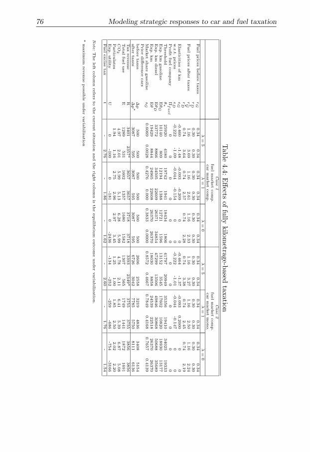
to make all car related taxes fully dependent on car use.6 I simulate the effects

of this move from lump-sum vehicle tax to tax on car use (‘variabilisation’)

for Cases 1 and 2. I set τD = τG = ∆β = 0, retain the VAT tax (i.e. tvat),

and then choose t ≡ tG = tD such that the taxation generates the same

total tax revenues as in the tax base scenario. Since the favorable purchase

tax treatment for gas cars disappears in this tax schedule, I eliminate the

favorable diesel fuel tax treatment in the new policy scenario by imposing

tG = tD; if the favorable diesel fuel tax treatment would be retained, the

share of gasoline cars would be essentially zero. Table 4.4 reports the effects

of such a policy. In Case 1 with a low price sensitivity (λ = 1), consumer

fuel prices under variabilisation would more than double, while the share of

gasoline car owners would essentially vanish. The total number of kilometers

decreases, but as a consequence of substitution towards diesel only by about

10 percent. Total fuel use decreases by 15 percent, as a consequence of both

the lower number of kilometers and the higher diesel fuel efficiency. Due to

the substitution towards diesel, the emission of particulates rises by 8%.

In Case 1 with a high price sensitivity (λ = 5) it appears not to be

possible to generate the same tax revenues under variabilisation. The higher

consumer fuel price generates a strong decrease in the number of kilometers,

the effect of which on total revenues is stronger than the effect of the higher

per liter revenue. The maximum revenue that can be obtained in this case is

two thirds of the revenue in the tax base scenario; the consumer fuel prices

are then three to five times as high as the consumer fuel prices in the tax

base scenario. Case 2 shows similar patterns for the two different values of

the price sensitivity parameter.

If the price sensitivity of kilometrage is sufficiently low, the variabilisation

policy has the possibility of inducing a tax revenue neutral shift towards lower

a kilometrage and a more fuel efficient engine type. On the other hand, it also

implies a drop in expected consumer utility. Note, however, that the model

does not account for the possibly positive effect of lower aggregate emissions

on consumer utility.

Note that by using the model in Verboven (2002) (λ = 0) I would have

underestimated the size of the excise on fuel. Also in this case it is always

possible to generate the same tax revenues under variabilisation.

6The European Parliament requested the abolishment of purchase taxes on cars in or-der to ‘increase competitiveness of car markets between EU countries’ (NRC Handelsblad,November 7, 2003).

76 Modeling strategic responses to car and fuel taxation

Table

4.4

:E

ffects

offu

llykilom

etrage-based

taxatio

nCase

1Case

2

fuelm

ark

et

com

p.

fuelm

ark

et

com

p.

car

mark

et

com

p.

car

mark

et

mono.

λ=

5λ

=1

λ=

0λ

=5

λ=

1λ

=0

Fuelpric

es

befo

reta

xes

rG

0.3

40.3

40.3

40.3

40.3

40.3

40.3

40.3

40.3

40.3

40.3

40.3

4r

D0.3

00.3

00.3

00.3

00.3

00.3

00.3

00.3

00.3

00.3

00.3

00.3

0Fuelpric

es

afte

rta

xes

r∗G

1.1

63.6

91.1

62.6

11.1

62.3

31.1

63.2

71.1

62.5

01.1

62.2

4r∗D

0.7

43.6

40.7

42.5

70.7

42.2

80.7

43.3

80.7

42.4

50.7

42.1

9Ela

sticitie

sofkm

eG

-0.4

60

-1.4

8-0

.093

-0.2

09

00

-0.4

64

-1.3

7-0

.093

0.2

000

00

w.r.t.

pric

es

eD

-0.2

22

-1.0

9-0

.044

-0.1

54

00

-0.2

22

-1.0

1-0

.044

-0.1

47

00

Pro

fit

fuelcom

pany

Πf

ue

l0

00

00

00

00

00

0T

hre

shold

θ∗

25920

4180

19742

1941

18434

1806

41797

20949

35356

19410

34025

19333

Exp.km

gaso

line

Eθ

G10140

809

12194

1388

12721

1596

13152

3545

17602

10820

18930

13177

Exp.km

die

sel

Eθ

D33772

8866

34505

22609

26371

34854

47299

13506

49846

30868

50688

35689

Exp.km

Eθ

19429

8844

24965

22608

26370

26370

18030

8858

24539

22518

26370

26370

Mark

et

share

gaso

line

sG

0.6

069

0.0

028

0.4

276

0.0

00

0.3

833

0.0

000

0.8

572

0.4

667

0.7

849

0.4

168

0.7

657

0.4

139

Pric

ediff

ere

nce

cars

befo

reta

xes

∆p

500

500

500

500

500

500

2606

2558

3219

4836

3408

5154

afte

rta

xes

∆p∗

3087

595

3087

595

3087

595

6726

3042

7785

5750

8111

6136

Tax

revenue

R3401

2357*

3657

3657

3718

3718

3393

2349*

3755

3755

3856

3856

Tota

lfu

eluse

E1289

531

1602

1357

1680

1582

1307

565

1749

1441

1872

1691

CO

24.9

72.0

15.9

95.1

36.2

85.9

94.7

82.1

16.4

15.3

96.8

75.0

8Partic

ula

tes

1.9

41.1

62.7

52.9

62.9

73.4

51.2

51.0

01.8

52.5

02.0

22.2

0Exp.utility

U0

-100

0-1

81

0-2

436

-134

-252

-259

-686

-754

-3166

Fuelexcise

tax

t-

2.7

6-

1.8

6-

1.6

2-

2.6

0-

1.7

6-

1.5

4

Note

:T

he

left

colu

mn

refe

rsto

the

curre

nt

situatio

nand

the

right

colu

mn

isth

eequilib

rium

outc

om

eunder

varia

bilisa

tion.

*m

axim

um

revenue

possib

leunder

varia

bilisa

tion

Chapter 4 77

4.6 Concluding remarks

The analysis of car and fuel taxation is complicated by the many interactions

between the actors involved: consumers, car producers, fuel producers and

the government. This Chapter has provided a coherent framework in which

these interactions are made explicit. The analysis emphasizes that optimal

tax rates do not only depend on the precise form of the government’s objective

function and the empirical values of the model parameters; the market forms

in both the fuel and the car market are essential as well.

As an application of the model, I analyzed the effects of a move of lump-

sum vehicle taxation toward taxing vehicle use. If the price sensitivity of

kilometrage is sufficiently low, such a variabilisation policy can induce a tax

revenue neutral shift towards lower kilometrage and a larger share of the

more fuel efficient engine type. Both these effects reduce fuel use and CO2-

emissions, but due to the substition towards diesel-powered cars particulate

emissions will increase. If the price sensitivity is relatively high full variabil-

isation may not be possible without a loss of tax revenues.

Another potential application of the model is to analyze the effects of an

increase in fuel production costs, for example as a result of increased crude oil

prices. Goel and Nelson (1999) provide empirical evidence that in such cases

governments tend to lower fuel taxes in order to mitigate the effect of the

price increase for consumers. I consider the extension of the present model to

allow for endogenous government behavior – possibly in a vote-maximization

framework – as a challenging further step toward a coherent analysis of car

and fuel taxation.

78 Modeling strategic responses to car and fuel taxation

4.A Derivation of the indirect utility function

Consumers receive extra utility when they drive more, other things equal.

This can be incorporated in two equivalent ways: assume a demand function

for kilometrage and derive (indirect) utility from the demand function or

assume a utility function dependent on the amount of kilometers consumed

and then derive the demand function and the indirect utility.

4.A.1 Starting point: a utility function

Let (j, k) be given, then the utility of the consumer depends on the expen-

diture on other goods (z) as a function of θjk and the utility received from

consuming θjk. If y∗ = y−ρp∗jk−τjk, then z = y∗−πjkθ

jk. The utility received

from consuming θjk is f(θj

k), where f(·) > 0, f(·)′ > 0 and f(·)′′ < 0. Utility

is given by:

ujk(θjk) = y∗ − πjkθ

jk + ajk + f(θj

k). (4.19)

Maximize with respect to θjk:

dujk(θjk)

dθjk

= −πjk + f ′(θjk) = 0 =⇒ f ′(θj

k) = πjk. (4.20)

From (4.20) follows the demand function of θjk. Substituting the demand

function in (4.19) gives the indirect utility.

4.A.2 Starting point: a demand function

Suppose the demand function of θjk is given by:

θjk = θj

0e−λπjk , (4.21)

where θj0 and λ are parameters. Note that if the variable costs are zero,

the consumer will drive θj0 kilometers. So, θj

0 is the maximum amount of θjk

the consumer will ‘purchase’. Substituting (4.21) in (4.19) gives the indirect

utility, but only if the function f(·) is chosen in such a way that the demand

function that follows from (4.20) is the same as the demand function given

in (4.21).

4.A.3 Equivalence

From (4.21) follows:

πjk =log θj

k − log θj0

−λ= − 1

λ[log θj

k − log θj0]. (4.22)

Chapter 4 79

Substituting this into (4.20) gives:

f ′(θjk) = − 1

λ[log θj

k − log θj0]. (4.23)

Integrating over θjk:

f(θjk) = − 1

λ

∫

[log θjk − log θj

0]dθjk = − 1

λ[θj

k log θjk − θj

k − θjk log θj

0]. (4.24)

After some rearranging the following is obtained:

f(θjk) = −θj

k

λ[log

(

θjk

θj0

)

− 1]. (4.25)

From θjk/θj

0 ≤ 1 it follows that f > 0. Note that f ′(θjk) = (−1/λ)[log θj

k −log θj

0] > 0 and f ′′(θjk) = −1/(λθj

k) < 0. Substitute (4.21) and (4.25) in (4.19)

to obtain the indirect utility function given in (4.1).

I would like to end by making some remarks about the function f(·):

1. f(0) = −∞

2. f(θj0e) = 0

3. f ′(θj0) = 0 and f(θj

0) = θj0/λ > 0.

This implies, that ∀θ ∈ [0, θj0] f ′(θ) ≥ 0 and ∀θ ∈ (θj

0, θj0e] f ′(θ) < 0. Since

f ′(θjk) = πjk and πjk is finite and non-negative, θj

k ∈ (0, θj0].

4.B Normalizing utility

The starting point in (4.1) is:

ujk = y − ρp∗jk − τjk + ajk +1

λe−λπjkθj

0 + vj . (4.26)

For convenience I drop the j subscript and the error term vj :

uk = y − ρp∗k − τk + ak +1

λe−λπkθ0. (4.27)

Suppose we have two scenarios. In the first scenario, the after tax sales price

of a car is p∗,Ik and the price of fuel is πIk. In the second scenario, the after tax

sales price of a car is p∗,IIk and the price of fuel is πII

k . It is always possible

80 Modeling strategic responses to car and fuel taxation

to normalize the utility in one of the scenarios to zero. Suppose utility in

scenario II is equal to zero. It follows that utility in the first scenario now is:

y − ρp∗,Ik − τk + ak +1

λe−λπI

kθ0 − y + ρp∗,IIk + τk − ak − 1

λe−λπII

k θ0 =

(4.28)

ρ(p∗,IIk − p∗,Ik ) +

θ0

λ[e−λπI

k − e−λπIIk ] ≡ ∆u

(4.29)

As long as λ > 0, the calculation of ∆u is straightforward. Suppose λ = 0.

Then the difference in utility is:

limλ→0

∆u = ρ(p∗,IIk − p∗,Ik ) + θ0 lim

λ→0

e−λπIk − e−λπII

k

λ(4.30)

= ρ(p∗,IIk − p∗,Ik ) + θ0 lim

λ→0[−πI

ke−λπI

k + πIIk e−λπII

k ] (4.31)

= ρ(p∗,IIk − p∗,Ik ) + θ0[π

IIk − πI

k] < ∞. (4.32)

Note that the difference in utility is just the difference in annualized car price

plus the difference in fuel cost evaluated in θ0. This is a consequence of the

quasi-linear utility and the fact that if λ = 0, then a person will always drive

θ0.

4.C The lognormal distribution

If θ0 ∼ LN(µ, σ2), then log θ0 ∼ N(µ, σ2). Let Φ(.|µ, σ2) denote the c.d.f. of

a normal distribution with mean µ and variance σ2. Then:

F (θ∗) = Pr(θ0 < θ∗) = Φ(log θ∗|µ, σ2) (4.33)

and

f(θ∗) =1

θ∗σ√

2πexp

[

−1

2

(

log θ∗ − µ

σ

)2]

. (4.34)

The required expressions for the expectation of θ0 conditional on fuel type

are

E(θ0|θ0 < θ∗) = exp(µ +1

2σ2) × Φ(log θ∗|µ + σ2, σ2)

Φ(log θ∗|µ, σ2)(4.35)

and

E(θ0|θ0 > θ∗) = exp(µ +1

2σ2) × 1 − Φ(log θ∗|µ + σ2, σ2)

1 − Φ(log θ∗|µ, σ2). (4.36)

See, for example, Aitchison and Brown (1957).