Embed Size (px)
Citation preview
UNIVERSITY OF CALIFORNIARIVERSIDE
Measurement of The Single Top Quark Production Cross Section at√s=1.96 TeV
A Dissertation submitted in partial satisfactionof the requirments for the degree of
Doctor of Philosphy
in
Physics
by
Mark Anthony Padilla
December 2011
Dissertation Commitee:Dr. Stepen Wimpenny, ChairpersonDr. Robert ClareDr. Jose Wudka

Copyright byMark Anthony Padilla
2011

The Dissertation of Mark Anthony Padilla is approved:
Committee Chairperson
University of California, Riverside

Acknowledgments
I would first and foremost like to thank my mother and father Cecilia and Rumaldo
Padilla for their love and support throughtout the years. None of this would have
been possible without them. Secondly, I would like to thank my wife Mehgan for
all her support throughtout the past six years, thankyou honey, I love you. I would
especially like to thank my advisor Stepen Wimpenny for all his guidance and support
and in helping me undertand many of the topics related to particle physics, thanks a
million Steve.
I would like to give special thanks to the Single Top Group at Fermilab for all
their help and support throughout the years. Liang, thanks for always being willing
to help with root, C++ ect., your helped me more than you know. Victor, thanks
for always pushing me and always having the time to help with code and many other
things related to the single top group. Reinhard, thankyou for your help and always
giving me clear and proper direction relative to the task at hand. Ann, thankyou for
always being more than willing to help and for some hard lessons learned. Cecilia,
thanks for keeping us on track with the big picture and helping us realize what needs
to be done. Nathan, thanks for helping me trouble shoot those annoying pieces of
code and collaborating with me on the BDTs. Jyoti, Wiegang and Yun-Tse thanks
for always being more than willing to help and the hard work all three of you have
put into the group, good luck in the future.
iv

As for my peers and teachers that have had a direct influence on helping me gain a
greater understanding of physics I would like to thank Medina, Gordon, Bob, Ryan,
George, Ben, Tim, Kathy, Dennis, Gil, Santino, Vince and Bruce, thanks for the
inspiration!
v

To Rumaldo Padilla 1940 - 2006,
the best father ever.
vi

ABSTRACT OF THE DISSERTATION
Measurement of The Single Top Quark Production Cross Section at√s=1.96 TeV
by
Mark Anthony Padilla
Doctor of Philosophy, Graduate Program in Physics
University of California, Riverside, December 2011
Dr. Stephen Wimpenny, Chairperson
Within the standard model top quarks are predicted to be most often produced in
pairs via the strong interaction. However they can also be produced singly through
the weak interation. This is a rarer process with many experimental challenges. It is
interesting because it provides a new window to search for evidence of physics beyond
the standard model picture, such as a fourth generation of quarks or to search for
insight into the Higgs Mechanism. Single top production also provides a direct way
to calculate the CKM matrix element Vtb.
This thesis presents new measurements for single top quark production in the
s+ t, s and t channels using 5.4 fb−1 of data collected at the DØ detector at Fermilab
in Batavia, IL. The analysis was performed using Boosted decision trees to separate
signal from background and Bayesian statistcs to calculate all the cross sections. The
results obtained are:
s channel : σ(pp→tb+X) = 0.68+0.41−0.39 pb,
t channel : σ(pp→tqb+X) = 3.03+0.78−0.66 pb,
Combined s+ t channels : σ(pp→tb+X, tqb+X) = 3.01+0.80−0.75 pb.
vii

The s channel has a Gaussian significance of 1.6σ, the t channel 5.5σ and the
s + t 4.3σ. The results are consistent with the standard model predictions within
one standard deviation. By combining these results with the results for two other
analyses (using different MVA techniques) improved results of:
Combined s+ t channels : σ(pp→tb+X, tqb+X) = 3.43+0.73−0.74 pb,
t channel : σ(pp→tqb+X) = 2.90+0.59−0.59 pb,
were obtained. These give a 5.6σ significance for the combined s+ t channel and 5.5σ
for the t channel.
viii

Contents
Acknowledgments iv
Dedication vi
Abstract vii
List of Tables ix
List of Figures x
1 Introduction 1
2 Theory 3
2.1 The Standard Model . . . . . . . . . . . . . . . . . . . . . . . . . . . 3
2.1.1 Particles . . . . . . . . . . . . . . . . . . . . . . . . . . . . . . 3
2.1.2 Forces . . . . . . . . . . . . . . . . . . . . . . . . . . . . . . . 4
2.1.3 Gauge Theories . . . . . . . . . . . . . . . . . . . . . . . . . . 4
2.2 The Top Quark . . . . . . . . . . . . . . . . . . . . . . . . . . . . . . 6
2.2.1 Top Quark Production . . . . . . . . . . . . . . . . . . . . . . 7
2.2.2 Pair Production . . . . . . . . . . . . . . . . . . . . . . . . . . 7
2.3 Single Top Quark . . . . . . . . . . . . . . . . . . . . . . . . . . . . . 11
ix

2.3.1 Introduction . . . . . . . . . . . . . . . . . . . . . . . . . . . . 11
2.3.2 Production . . . . . . . . . . . . . . . . . . . . . . . . . . . . 11
2.3.3 Signal and Background . . . . . . . . . . . . . . . . . . . . . . 12
2.3.4 CKM Matrix Element |Vtb| . . . . . . . . . . . . . . . . . . . . 14
2.3.5 Polarization . . . . . . . . . . . . . . . . . . . . . . . . . . . . 16
2.3.6 Beyond The Standard Model . . . . . . . . . . . . . . . . . . . 16
3 Accelerators and Detectors 18
3.1 Introduction . . . . . . . . . . . . . . . . . . . . . . . . . . . . . . . . 18
3.2 Cockroft-Walton Pre-accelerator . . . . . . . . . . . . . . . . . . . . . 19
3.3 Linear Accelerator (Linac) . . . . . . . . . . . . . . . . . . . . . . . . 21
3.4 Proton Booster Ring . . . . . . . . . . . . . . . . . . . . . . . . . . . 21
3.5 Fermilab Main Injector . . . . . . . . . . . . . . . . . . . . . . . . . . 21
3.6 Antiproton Production . . . . . . . . . . . . . . . . . . . . . . . . . . 22
3.7 Tevatron . . . . . . . . . . . . . . . . . . . . . . . . . . . . . . . . . . 23
3.8 DØ Detector . . . . . . . . . . . . . . . . . . . . . . . . . . . . . . . 24
3.8.1 DØ Coordinate System . . . . . . . . . . . . . . . . . . . . . . 24
3.8.2 Central Tracking System . . . . . . . . . . . . . . . . . . . . . 26
3.8.3 DØ Calorimeters . . . . . . . . . . . . . . . . . . . . . . . . . 30
3.8.4 Muon Detectors . . . . . . . . . . . . . . . . . . . . . . . . . . 33
3.8.5 Luminosity Monitor . . . . . . . . . . . . . . . . . . . . . . . 34
3.9 Trigger Framework . . . . . . . . . . . . . . . . . . . . . . . . . . . . 36
4 Event Reconstruction 39
4.1 Charged Track Reconstruction . . . . . . . . . . . . . . . . . . . . . . 39
4.2 Primary Vertex . . . . . . . . . . . . . . . . . . . . . . . . . . . . . . 41
4.3 Electron Identification . . . . . . . . . . . . . . . . . . . . . . . . . . 42
x
4.4 Muon Reconstruction . . . . . . . . . . . . . . . . . . . . . . . . . . . 45
4.5 Jet Reconstruction . . . . . . . . . . . . . . . . . . . . . . . . . . . . 46
4.5.1 Calibration of the Jet Energy Scale . . . . . . . . . . . . . . . 48
4.5.2 b-Jet Identification . . . . . . . . . . . . . . . . . . . . . . . . 51
4.6 Reconstruction of Missing Transverse Energy, /ET . . . . . . . . . . . 52
5 Data Samples and Event Selection 55
5.1 The RunII Data Sample . . . . . . . . . . . . . . . . . . . . . . . . . 55
5.2 Simulated Event Samples . . . . . . . . . . . . . . . . . . . . . . . . . 56
5.2.1 Simulation of Single Top Signal . . . . . . . . . . . . . . . . . 57
5.2.2 Background Event Simulation . . . . . . . . . . . . . . . . . . 57
5.3 Modeling the QCD Multijet Background . . . . . . . . . . . . . . . . 61
5.4 The Effects of the Top Mass Uncertainty . . . . . . . . . . . . . . . . 61
5.5 Determination of the W+Jets and Multijet Background Normilizations 62
5.6 Event Selection . . . . . . . . . . . . . . . . . . . . . . . . . . . . . . 64
5.6.1 General Preselection Requirements . . . . . . . . . . . . . . . 64
5.6.2 Electron+Jets Channel Preselection . . . . . . . . . . . . . . . 66
5.6.3 Muon+Jets Channel Preselection . . . . . . . . . . . . . . . . 67
5.7 Analysis Subsamples and Preliminary Data-Simulation Comparisions 69
6 Monte Carlo Model Corrections and Statistical Uncertainties 74
6.1 Detector Response Corrections . . . . . . . . . . . . . . . . . . . . . . 74
6.2 Theoretical Uncertainties . . . . . . . . . . . . . . . . . . . . . . . . . 78
6.3 Residual Systematic Uncertainties . . . . . . . . . . . . . . . . . . . . 80
6.3.1 Normalization Effects . . . . . . . . . . . . . . . . . . . . . . . 82
6.3.2 Shape-changing Effects . . . . . . . . . . . . . . . . . . . . . . 85
6.3.3 Summary of Residual Uncertainties . . . . . . . . . . . . . . . 87
xi
7 Boosted Decision Trees 89
7.1 Introduction . . . . . . . . . . . . . . . . . . . . . . . . . . . . . . . . 89
7.2 Sample Preparation . . . . . . . . . . . . . . . . . . . . . . . . . . . . 92
7.3 Training . . . . . . . . . . . . . . . . . . . . . . . . . . . . . . . . . . 92
7.3.1 Splitting a Node . . . . . . . . . . . . . . . . . . . . . . . . . 93
7.3.2 Boosting . . . . . . . . . . . . . . . . . . . . . . . . . . . . . . 94
7.3.3 Parameters . . . . . . . . . . . . . . . . . . . . . . . . . . . . 95
7.3.4 Implementation . . . . . . . . . . . . . . . . . . . . . . . . . . 97
7.3.5 Selection of Input Variables . . . . . . . . . . . . . . . . . . . 97
7.4 Transformation of the BDT Discriminant . . . . . . . . . . . . . . . . 107
7.5 Background Cross Checks . . . . . . . . . . . . . . . . . . . . . . . . 109
8 Analysis 112
8.1 Cross Section Measurment . . . . . . . . . . . . . . . . . . . . . . . . 112
8.1.1 Bayesian Approach . . . . . . . . . . . . . . . . . . . . . . . . 113
8.1.2 Systematic Uncertainties . . . . . . . . . . . . . . . . . . . . . 115
8.2 Results . . . . . . . . . . . . . . . . . . . . . . . . . . . . . . . . . . . 116
8.2.1 Expected Results . . . . . . . . . . . . . . . . . . . . . . . . . 116
8.2.2 Observed Results . . . . . . . . . . . . . . . . . . . . . . . . . 118
8.3 Ensemble Tests . . . . . . . . . . . . . . . . . . . . . . . . . . . . . . 122
8.3.1 Significance . . . . . . . . . . . . . . . . . . . . . . . . . . . . 126
8.3.2 Asymptotic approximation of the log-likelihood ratio . . . . . 126
8.3.3 Measured Significance . . . . . . . . . . . . . . . . . . . . . . 127
8.4 |Vtb| Measurement . . . . . . . . . . . . . . . . . . . . . . . . . . . . . 130
9 Comparison of Results 132
9.1 DØ and CDF Measurements . . . . . . . . . . . . . . . . . . . . . . . 132
xii

9.1.1 Comparisons . . . . . . . . . . . . . . . . . . . . . . . . . . . 133
10 Conclusions 139
A Decision Tree Outputs 141
B Residual Systematic Errors 145
B.1 Normalization Uncertainties . . . . . . . . . . . . . . . . . . . . . . . 145
B.2 Shape and Normalization Uncertainties . . . . . . . . . . . . . . . . . 149
Bibliography 156
xiii

List of Tables
2.1 Elementary Particles and their properties. . . . . . . . . . . . . . . . 4
2.2 Top quark branching fractions [7] . . . . . . . . . . . . . . . . . . . . 7
2.3 On mass shell W boson branching ratios [8] . . . . . . . . . . . . . . 8
2.4 QCD prediction for the NLO cross section for single top quark produc-
tion at√s=1.96TeV . . . . . . . . . . . . . . . . . . . . . . . . . . . 12
4.1 Definitions for three classes of electron candidates. . . . . . . . . . . . 45
5.1 Luminosity breakdown of the Run II dataset as a function of trigger
version. . . . . . . . . . . . . . . . . . . . . . . . . . . . . . . . . . . 56
5.2 Sizes of the signal and background simulated event samples. The labels
Run IIa and Run IIb, denote that these events were reconstructed with
the software used for the data from these subsets of the data. . . . . . 58
5.3 Fitted W+Jets and QCD Multijet Scale Factors for each of the 24 fits. 63
5.4 Comparison of observered and predicted yields for the the single tagged
event samples. . . . . . . . . . . . . . . . . . . . . . . . . . . . . . . . 70
5.5 Comparison of observered and predicted yields for the the double tagged
event samples. . . . . . . . . . . . . . . . . . . . . . . . . . . . . . . . 71
xiv
6.1 Residual systematic uncertainties after improvements to detector and
process simulations. Where ranges are given, these correspond to 2, 3
and 4 jet events. . . . . . . . . . . . . . . . . . . . . . . . . . . . . . . 88
7.1 List of individual object kinematics. . . . . . . . . . . . . . . . . . . . 100
7.2 List of event variables. . . . . . . . . . . . . . . . . . . . . . . . . . . 100
7.3 List of variables using the sign of lepton charge. . . . . . . . . . . . . 100
7.4 Calculated mass, pT and the HT variables. . . . . . . . . . . . . . . . 101
7.5 Reconstructed top quark variables. . . . . . . . . . . . . . . . . . . . 101
7.6 Reconstructed W boson variables. . . . . . . . . . . . . . . . . . . . . 102
7.7 Angular Correlations. . . . . . . . . . . . . . . . . . . . . . . . . . . . 102
8.1 Expected cross sections for s+t, s and t channels in pb. . . . . . . . . 118
8.2 Expected posterior peak over half-width ratios for s+t, s and t channels.118
8.3 Expected cross sections in individual analysis channels (e,µ) combined. 119
8.4 Observed cross sections for s+t, s and t channels in pb. . . . . . . . . 119
8.5 Observed posterior peak over half-width ratios for s+t, s and t channels.119
8.6 Observed cross sections in individual analysis channels (e,µ) combined. 120
8.7 Cross section inputs for each individual channel. . . . . . . . . . . . . 122
8.8 Parameters of the likelihood which are used in the calculation of the
significances using the AALR approach. . . . . . . . . . . . . . . . . . 128
8.9 Expected and observed results for the single top cross sections. . . . . 130
9.1 DØ significance results for s+ t, s and t channels. . . . . . . . . . . . 135
9.2 DØ and CDF significance results for s+ t, s and t channels. . . . . . 137
B.1 Residual normalization systematic uncertainties: two jets with 1-btag.
These values are used as input parameters to the BDT analysis. . . . 146
xv

B.2 Residual normalization systematic uncertainties: two jets with 2-btags.
These values are used as input parameters to the BDT analysis. . . . 146
B.3 Residual normalization systematic uncertainties: three jets with 1-btag.
These values are used as input parameters to the BDT analysis. . . . 147
B.4 Residual normalization systematic uncertainties: three jets with 2-
btags. These values are used as input parameters to the BDT analysis. 147
B.5 Residual normalization systematic uncertainties: four jets with 1-btag.
These values are used as input parameters to the BDT analysis. . . . 148
B.6 Residual normalization systematic uncertainties: four jets with 2-btags.
These values are used as input parameters to the BDT analysis. . . . 148
xvi

List of Figures
2.1 The fundamental particles and their interactions [2]. The lines con-
necting the particles indicate which interaction can take place. . . . . 5
2.2 Feynman diagrams for tt production. The top diagram shows quark-
antiquark annihilation, the bottom three show gluon fusion [9]. . . . 9
2.3 Pie chart representing all branching fractions for for tt pair events [9]. 10
2.4 Feynman diagram at LO for t-channel production. . . . . . . . . . . . 12
2.5 Feynman diagram at LO for s-channel production. . . . . . . . . . . . 13
2.6 Feynman diagrams for background processes related to single top quark
production. W+jets (top-left), Z+jets(top-right), tt(middle-left), Diboson(middle-
right) and QCD multijets (bottom). . . . . . . . . . . . . . . . . . . . 15
2.7 Feynman diagrams showing BSM processes through the s-channel (left)
and t-channel (right) single top quark production. . . . . . . . . . . . 17
3.1 Diagram of Fermilab’s chain of accelerators. . . . . . . . . . . . . . . 18
3.2 (a) The Cockroft-Walton Accelerator. (b) Voltage multiplier circuit
diagram. . . . . . . . . . . . . . . . . . . . . . . . . . . . . . . . . . . 20
3.3 H− ion production in the magnetron. . . . . . . . . . . . . . . . . . . 20
3.4 Schematic diagram of the Target and Lens system. [19]. . . . . . . . . 23
xvii

3.5 Schematic of the experimental hall and the DØ detector. The location
of each of the major subsystems is shown, along with the position of
the on-detector readout electronics. . . . . . . . . . . . . . . . . . . . 25
3.6 DØ coordinate system. . . . . . . . . . . . . . . . . . . . . . . . . . . 25
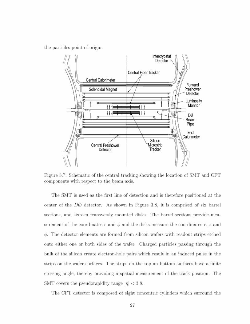
3.7 Schematic of the central tracking showing the location of SMT and
CFT components with respect to the beam axis. . . . . . . . . . . . . 27
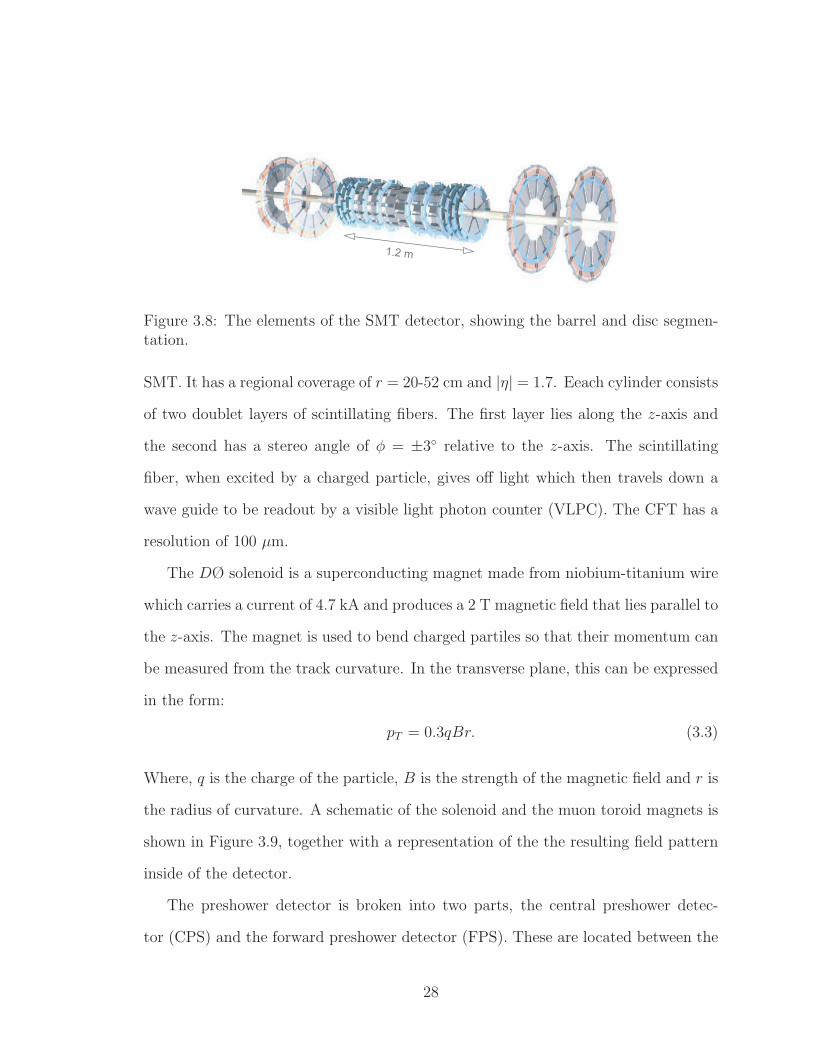
3.8 The elements of the SMT detector, showing the barrel and disc seg-
mentation. . . . . . . . . . . . . . . . . . . . . . . . . . . . . . . . . . 28
3.9 Schematic representation of the DØ magnets and the magnetic field
within the detector volume. . . . . . . . . . . . . . . . . . . . . . . . 29
3.10 Schematic diagram shown the DØ central endcap calorimeters. The
cut away shows the details of the calorimeter modules [26]. . . . . . 30
3.11 Depiction of a photon shower where X◦ represents one radiation length. 31
3.12 Structure of a unit cell in the liquid Ar calorimeter modules. . . . . . 32
3.13 Schematic of one octant of the DØ central and encap calorimeters.
The shaded regions show the projective structure of the calorimeter
towers and their map onto pseudorapidity. . . . . . . . . . . . . . . . 33
3.14 Exploded view of the DØ muon detection system. The top diagram
shows the the configuration of the A, B and C layers in the barrel and
forward regions. The bottom diagram shows the location of the barrel
and forward scintillation counters. . . . . . . . . . . . . . . . . . . . . 35
3.15 Diagram of the Luminosity monitors at DØ [26]. . . . . . . . . . . . . 36
3.16 Block diagram of the DØ framework, showing the data-flow through
the three levels of the trigger. . . . . . . . . . . . . . . . . . . . . . . 37
xviii
3.17 Block diagram of L1 and L2 showing what systems they are connected
to [26]. All detectors are listed on the left where the calorimeter (CAL)
is initially connected to the level 1 trigger, the central tracking trig-
ger (CTT) is defined as both the preshower detectors (CPS and FPS)
and the fiber tracker (CFT) and is also connected to the L1 trigger.
The SMT goes straight to L2 where the muon system begins at L1.
The forward proton detector (FPD) and the Luminosity monitor are
also connected to L1 initally. . . . . . . . . . . . . . . . . . . . . . . . 38
4.1 Diagram of track reconstruction using the AA algorithm. . . . . . . . 41
4.2 Schematic of the parton fragmentation process and the particle show-
ering used to detect the fragmentation products in the calorimeters. . 48
4.3 Fη measurements as a function of η for |η| < 3.5. . . . . . . . . . . . . 50
4.4 Diagram of the MPF method for a γ + jet event. . . . . . . . . . . . 51
4.5 Schematic of a 3-jet event in which one of the jets originates from a
b-quark and has a displaced secondary vertex. The origin of the non-
tagged jets is consistent with the primary vertex. . . . . . . . . . . . 53
5.1 Lowest order Feynman diagrams for the s and t channel signal processes
and the principle backgrounds. . . . . . . . . . . . . . . . . . . . . . . 60
5.2 Triangle cut in the |∆φ(leading jet, /ET)| vs. /ET plane. . . . . . . . . . 65
5.3 Triangle cut in the second leading jet pT vs. HT (alljets) plane. . . . . 66
5.4 Triangle cuts in the /ET vs. |∆φ(e, /ET )| plane. . . . . . . . . . . . . . 67
5.5 Triangle cuts in the /ET vs. |∆φ(µ, /ET)| plane. . . . . . . . . . . . . . 69
5.6 Colour scheme plot key used to label Data, siganl and background
events for plots. . . . . . . . . . . . . . . . . . . . . . . . . . . . . . . 72
xix

5.7 Comparison of the observed and predicted yields for 15 of the kinematic
variables used as inputs to the BDT. . . . . . . . . . . . . . . . . . . 73
6.1 The two plots on the left are εfake−e and QCDWeight = εfake−e/(1 −
εfake−e). The two on the right are the same thing with the real electron
contamination subtracted out. . . . . . . . . . . . . . . . . . . . . . . 81
6.2 The plot on the left has no correction whereas the plot on the right
has been corrected. . . . . . . . . . . . . . . . . . . . . . . . . . . . . 81
7.1 Schematic of a decision tree showing the effects of branching and the
terminal leaves. The blue circles represent nodes which are split into
daughter nodes. Each daughter node is subjected to an independent
test to see wether it will contiue to be split or end as a terminal
leaf (green). Here F and P stand for fail and pass the nodal test. . . . 91
7.2 Example plots showing separation power and cross section significance
versus the number of boosts. . . . . . . . . . . . . . . . . . . . . . . . 96
7.3 Data-Simulation comparison for selected variables I. . . . . . . . . . . 103
7.4 Data-Simulation comparison for selected variables II. . . . . . . . . . 104
7.5 Data-Simulation comparison for selected variables III. . . . . . . . . . 105
7.6 Data-Simulation comparison for selected variables IV. . . . . . . . . . 106
7.7 Discriminant Transformation Histogram a.) is the raw distribution, b.)
is the transformed distribution and c.) is the transformation function. 108
7.8 BDT cross check samples for s+t, s and t where the histograms dom-
inated by red correspond to tt events and the green dominated ones
indicate W+Jet events. . . . . . . . . . . . . . . . . . . . . . . . . . . 110
xx

7.9 BDT cross check samples for s+t, s and t where the histograms dom-
inated by red correspond to tt events and the green dominated ones
indicate W+Jet events. . . . . . . . . . . . . . . . . . . . . . . . . . . 111
8.1 Representation of a 1D posterior density distribution where the peak of
the curve represents a cross section measurement and ∆σ its uncertainty.115
8.2 Representation of shape changing uncertainties. . . . . . . . . . . . . 116
8.3 Expected posterior density distributions for s+t (top left), s (top right)
and t (bottom). The results include both statistical and systematic
uncertainties. . . . . . . . . . . . . . . . . . . . . . . . . . . . . . . . 117
8.4 BDT output distributions for s+t, s and t channel analyses with all six
channels combined. The top row corresponds to the linear scale, the
middle the log scale and the bottom are zoomed plots showing signal
excess over background. . . . . . . . . . . . . . . . . . . . . . . . . . 120
8.5 Observed posterior density distributions for the single top s+t (top
left), s (top right) and t (bottom) analyses. . . . . . . . . . . . . . . . 121
8.6 Results of ensemble tests for the combined s+ t channel analysis. The
observed linear behavior indicates the absence of bias from the analysis
procedure. . . . . . . . . . . . . . . . . . . . . . . . . . . . . . . . . . 123
8.7 Results of ensemble tests for the combined s channel analysis. The
observed linear behavior indicates the absence of bias from the analysis
procedure. . . . . . . . . . . . . . . . . . . . . . . . . . . . . . . . . . 124
8.8 Results of ensemble tests for the combined t channel analysis. The
observed linear behavior indicates the absence of bias from the analysis
procedure. . . . . . . . . . . . . . . . . . . . . . . . . . . . . . . . . . 125
xxi
8.9 Probability density vs. log-likehood significance for the s + t channel
analysis. . . . . . . . . . . . . . . . . . . . . . . . . . . . . . . . . . . 128
8.10 Probability density vs. log-likehood significance for the s channel anal-
ysis. . . . . . . . . . . . . . . . . . . . . . . . . . . . . . . . . . . . . 129
8.11 Probability density vs. log-likehood significance for the t channel anal-
ysis. . . . . . . . . . . . . . . . . . . . . . . . . . . . . . . . . . . . . 130
8.12 Posterior densities for both |VtbfL1 |2 (left) and |Vtb|2 (right). . . . . . . 131
9.1 DØ cross section results for 2.3 fb−1, 5.4 fb−1. . . . . . . . . . . . . . 135
9.2 Cross section results for 2.3 fb−1 (DØ), 5.4 fb−1 (DØ) and 3.2 fb−1
(CDF) data sets. . . . . . . . . . . . . . . . . . . . . . . . . . . . . . 136
9.3 2D posterior density for BNN Combination t. Below are the 1D pos-
terior densities for both s and t obtained by integrating over both axes. 138
A.1 Boosted decision tree outputs for the s + t channel. The first row
consists of the once tagged 2,3 and 4 jet samples, the second row the
twice tagged 2,3 and 4 jet samples, the third row the 1-2 tagged 2,3
and 4 jet samples and the last row consists of the once tagged 2-4 jets
combined sample, the twice tagged 2-4 jets combined sample and the
combined sample of 1-2 tags and 2-4 jets. . . . . . . . . . . . . . . . . 142
A.2 Boosted decision tree outputs for the s channel. The first row consists
of the once tagged 2,3 and 4 jet samples, the second row the twice
tagged 2,3 and 4 jet samples, the third row the 1-2 tagged 2,3 and 4 jet
samples and the last row consists of the once tagged 2-4 jets combined
sample, the twice tagged 2-4 jets combined sample and the combined
sample of 1-2 tags and 2-4 jets. . . . . . . . . . . . . . . . . . . . . . 143
xxii

A.3 Boosted decision tree outputs for the t channel. The first row consists
of the once tagged 2,3 and 4 jet samples, the second row the twice
tagged 2,3 and 4 jet samples, the third row the 1-2 tagged 2,3 and 4 jet
samples and the last row consists of the once tagged 2-4 jets combined
sample, the twice tagged 2-4 jets combined sample and the combined
sample of 1-2 tags and 2-4 jets. . . . . . . . . . . . . . . . . . . . . . 144
B.1 Combined s+ t channel discriminant, showing the effects of a ±1 fluc-
tuation in each systematic. The plots are for events with a single b tag.
The left column is for the 2 jet events, the center column is for 3 jet
events and the right column is for 4 jet events. . . . . . . . . . . . . . 150
B.2 Combined s+ t channel discriminant, showing the effects of a ±1 fluc-
tuation in each systematic. The plots are for events with a two b tags.
The left column is for the 2 jet events, the center column is for 3 jet
events and the right column is for 4 jet events. . . . . . . . . . . . . . 151
B.3 Combined s channel discriminant, showing the effects of a ±1 fluctu-
ation in each systematic. The plots are for events with a single b tag.
The left column is for the 2 jet events, the center column is for 3 jet
events and the right column is for 4 jet events. . . . . . . . . . . . . . 152
B.4 Combined s channel discriminant, showing the effects of a ±1 fluctu-
ation in each systematic. The plots are for events with a two b tags.
The left column is for the 2 jet events, the center column is for 3 jet
events and the right column is for 4 jet events. . . . . . . . . . . . . . 153
xxiii

B.5 Combined t channel discriminant, showing the effects of a ±1 fluctua-
tion in each systematic. The plots are for events with a single b tag.
The left column is for the 2 jet events, the center column is for 3 jet
events and the right column is for 4 jet events. . . . . . . . . . . . . . 154
B.6 Combined t channel discriminant, showing the effects of a ±1 fluctu-
ation in each systematic. The plots are for events with a two b tags.
The left column is for the 2 jet events, the center column is for 3 jet
events and the right column is for 4 jet events. . . . . . . . . . . . . . 155
xxiv

Chapter 1
Introduction
It all started when I was eight years old with firecrakers and toy cars. I always won-
dered what toy cars were made of so I decided to use a firecraker to blow up the
minuature car to find out. After many attempts I finally accomplished my task with
a suitable sized firecraker (M-80), however I was not impressed. My experiment yieled
burnt plastic and charred metal. Years later I find that I’m still doing the same thing,
well, not demolishing toy cars but trying to figure out the fundamental constituent’s
of nature and their processes. The model that best describes the fundamental par-
ticles of nature and how those particles interact with one another is known as the
Standard Model (SM). The interactions between fundamental particles occur via the
four known forces of nature: electromagnetic, strong, weak and gravitaional. The
SM only incorporates the first three of these forces and it has been very successful in
describing nature and its interactions. However, like many theories it is still a work
in progress. One way to probe the limits of a theory is through the use of a high
energy particle accelerator.
The second largest particle accelerator in the world is the Tevatron which is located
at Fermilab in Batavia, IL. This is the machine that was used for the discovery of
1

the Top Quark in 1995 by the DØ and CDF collaborations. The discovery was huge,
because not only did it further validate the SM, but it also resulted in the observation
of the most massive fundamental particle ever observed. The top quark weighs in at
approximatley 172 GeV, which is over 170 times the mass of a proton. Because of its
large mass, the top quark makes a good starting point to search for theories beyond
the current standard model. In 1995 the discovery of the top quark was based on
the production of tt pairs through the strong force. More recently (2009) single top
quark production was observed for the first time. This proceeds through the weak
force in three production channels, called the s, t, and tW channels. This analysis
makes refined measurements of the combined s+t channel cross section, and separate
measurements of the s and t channel cross sections. The tW channel is not currently
measurable because of the large background coming from tt pair production, which
is kinematically almost indistinguishable.
This thesis presents the following chapters: Chapter 2 gives an overview of the
standard model and current theories relating to particle physics. Chapter 3 describes
the accelerator used to produce top quarks and the DØ detector which was used
to observe them. Chapter 4 discusses how objects such as electrons, muons and
other physics objects are reconstructed from a proton antiproton collision. Chapter
5 describes the data collection, signal and background modeling, and the basic event
selection. The corrections made to the Monte Carlo simulation and the systematic
uncertainties are discussed in Chapter 6. Chapters 7 and 8 discuss the use of Boosted
Decisions Trees to identify the signal and the measurement of the cross sections.
Lastly, Chapters 9 and 10 compare the results to previous measurements and the
predictions of theory.
2

Chapter 2
Theory
2.1 The Standard Model
2.1.1 Particles
In the Standard model the fundamental particles are divided into three categories
which are, Leptons, Quarks and Bosons. The leptons and quarks are fermions and
they both carry half integer spin. The bosons are the force carriers and they have
integer spin. The lepton and quark families are separated into three generations as
shown in Table 2.1. Each generation has two doublets: one of quarks and the second
of leptons associated with it. Each quark doublet consists of a particle with +2/3e
charge and a second particle with -1/3e charge whereas the lepton doublets have one
particle with +1e charge and a second which is neutral. The particle masses vary with
the first generation being the lightest and the third the heaviest. For each particle in
all generations there is an associated anti-particle with the same mass but opposite
charge. The particles in the first generation are the basic building blocks for the
known universe.
3

Quark Lepton
Generation Flavor Charge Mass(MeV/c2) Flavor Charge Mass(MeV/c2)I Up(u) +2/3e 7.5 Electron(e) -e 0.511
Down(d) -1/3e 4.2 Neutrino(νe) 0 <2.0×10⁻⁴
II Charm(c) +2/3e 1.1×10³ Muon(µ) -e 105Strange(s) -1/3e 150 Neutrino(νµ) 0 <0.19
III Top(t) +2/3e 173×103 Tau(tau) -e 1784Bottom(b) -1/3e 4.2×10³ Neutrino(ντ ) 0 <18.2
Table 2.1: Elementary Particles and their properties.
2.1.2 Forces
Whenever we look out into nature it is safe to say that we always observe things inter-
acting. This takes place via the four fundamental forces: gravity, electromagnetism,
weak and strong. Each force is transmitted through a mediating boson. In the case
of gravity, the boson is called the graviton. However theorists have had serious is-
sues reconciling general relativity with quantum mechanics, therefore gravity in not
included within our current standard model. The photon is the mediator particle for
the electromagnetic force and the mediators for the weak force are the W+, W− and
Z bosons. Gluons mediate the strong force. Last but not least is the Higgs Boson
which is predicted by the SM and is suppose to give rise to the particle mass. The
Higgs boson has not yet been observed, and there are on going searches taking place
at CERN (Large Hadron Collider) and Fermilab(Tevatron). These searches have ex-
cluded some of the mass regions where the Higgs could exist, however no siganl has
been observed sofar. A diagram of the particles and their associated interactions is
shown in Figure 2.1.
2.1.3 Gauge Theories
Gauge Theory is a mathematical model created by physicists in order to explain
the interactions of fermions. The field theory which combines the effects of special
4

Figure 2.1: The fundamental particles and their interactions [2]. The lines connectingthe particles indicate which interaction can take place.
relativity and quantum mechanics is known as quantum field theory (QFT). The main
concept behind a gauge theory is that the Lagrangian remains invariant for local and
global symmetry transformations where the global is just a subset of the local. The
theory began in the 1920’s when physicists were trying to create a quantum theory for
the electromagnetic interaction. This is now called quantum electrodynamics (QED).
If we extrapolate form the 1920’s to now, one of the most successful gauge theories
is the standard model of particle physics.
The gauge group SU(2)L × U(1)Y represents the electroweak interaction which
is the unifying group for the electromagnetic (U(1)) and weak interactions (SU(2)).
The subscript L points out that the weak force is associated with only left-handed
particles and Y signifies the weak hypercharge. The gauge group SU(3)C is associated
with the strong interaction where the C indicates color charge. Together these groups
form the standard model gauge group, SU(3)C × SU(2)L × U(1)Y .
One final note should be presented, that of “spontaneous symmetry breaking”. If
the symmetry of the gauge group SU(2)L × U(1)Y is to remain unbroken then this
5

requires that all its mediator particles be massles. Through experiment we have seen
that the W and Z bosons have masses of 80.4 Gev and 91.2 GeV [1]. To deal with this
inconsistency theorists created the “Higgs Mechanism”. This allows for the W and
Z bosons to have mass while preserving the theory. However the introduction of this
produces another particle called the Higgs Boson, which has not yet been observed.
2.2 The Top Quark
The roots of the top quark lie in a postulate made by Makoto Kobayashi and Toshihide
Maskawa in 1973. They were trying to understand CP violation in Kaon decays [3] by
introducing a new generation of quarks which is now known to be the third generation.
However, it was not until 1977 that one of the quarks in the third generation doublet,
the b quark, was discoverd [4]. Following the generational pattern of the SM the b
quark was predicted to have an isospin partner named the t or top quark. Some 18
years later the top quark was finally observed by the DØ and CDF collaborations [5].
The top quark is by far the heaviest particle in the SM model, weighing in at a
massive 172 GeV (∼170mproton). It is similar to the u and c quarks in that it is a
spin-1/2 particle and carries a charge of +2/3e. However, because the top quark is so
massive it decays very rapidly with a lifetime of ∼ 5× 10⁻²⁶s, which means it has no
time to hadronize before it decays. This special property allows physicists to study
the poloraization and the angular correlations related to its decay products. The top
quark interacts through both the strong and weak forces where the strong interaction
produces tt pairs and the weak interaction produces top quarks singly. Both these
production modes are discussed in the following sections. This thesis focuses on the
analysis of the single top quark production mode.
6

2.2.1 Top Quark Production
Currently, the Tevatron at Fermilab and the LHC at CERN are the only two particle
accelerators in the world capable of creating top quarks. Here, we will only focus on
top quarks created at Fermilab since this thesis is based on data taken from there.
The Tevatron creates top quarks by colliding a proton with an antiproton at a center
of mass energy of 1.96 TeV. There are two types of production modes: tt pairs and
single top quark production. Between these two, pair production dominates.
2.2.2 Pair Production
As mentioned earlier, the top quark was first observed in 1995 by the DØ and CDF
collaborations. It was obsereved in pairs, one top and one anti-top. The different
sub-processes in which tt production occurs is shown by the Feynman diagrams in
Figure 2.2. Of these, the top diagram (qq annihilation) is the dominant production
mode at the Tevatron. Currently, the tt production cross section is measured to be
7.78+0.77−0.64 [6]. The qq annhilation accounts for around 85% of the cross section, with
the remaining 15% coming from the gluon fusion processes (bottom three diagrams).
After the top quarks are created they decay very quickly to a W boson and a b quark
almost 100% of the time. The branching fractions for the top quark decay can be
seen in Table 2.2.
Decay Mode Branching Fractiont → Wd ∼ 0.006%t → Ws ∼ 0.17%t → Wb ∼ 99.8%
Table 2.2: Top quark branching fractions [7].
Clearly the t → Wb decay dominates. In this mode the b quark fragments into
7

a jet of particles while the W boson decays into a lepton and a neutrino or qq pair.
The branching ratios for W decay are shown in Table 2.3. All tt pair branching
Decay Mode Branching FractionW+ → eν (10.75±0.13)W+ → µν (10.57±0.15)W+ → τν (11.25±0.20)W+ → hadrons (67.60±0.27)
Table 2.3: On mass shell W boson branching ratios [8].
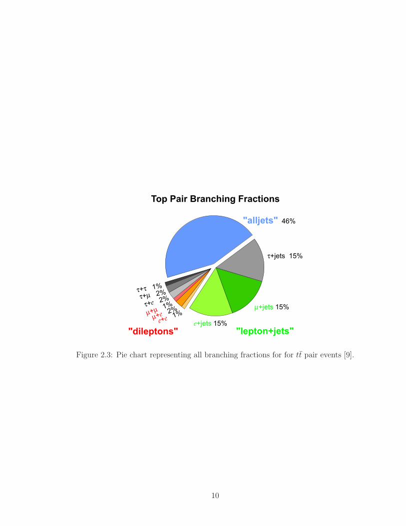
fractions are shown in Figure 2.3. The dilepton process accounts for 9% of all tt pair
production, 45% for lepton+jets and 46% for alljets.
8
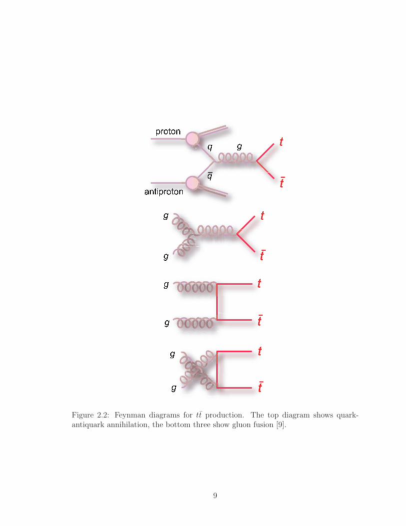
Figure 2.2: Feynman diagrams for tt production. The top diagram shows quark-antiquark annihilation, the bottom three show gluon fusion [9].
9
τ+τ 1%
τ+µ 2%
τ+e 2%
µ+µ 1%
µ+e 2%
e+e 1%
e+jets 15%
µ+jets 15%
τ+jets 15%
"alljets" 46%
"lepton+jets""dileptons"
Top Pair Branching Fractions
Figure 2.3: Pie chart representing all branching fractions for for tt pair events [9].
10

2.3 Single Top Quark
2.3.1 Introduction
Single top quark production is unlike tt pair production in that it does not occur
through the strong interaction but the weak, also we only get one top quark instead
of two. At the Tevatron this process occurs about once in every 10 billion events
making it a very difficult particle to detect. In 2009, the single top quark process was
first observed by the DØ and CDF collaborations [10], 14 years after the top quark
was first observed. This was quite a triumph in the physics community, not only
because it took a long time to find but because this opens up a new area for searches
for physics that may lie outside the SM. It also has allowed us to study different
properties associated with the top quark. The last three sections of this chapter is
devoted to a brief description of the properties of the top quark and Beyond the
standard model (BSM) searches.
2.3.2 Production
The single top quark is produced in three different channels, that is the t channel,
the s channel and the Wt channel. The latter channel has the smallest cross section
at the Tevatron and is neglected here because of this and its similarity to the tt state.
The t channel is the dominant channel follwed by the s channel. The next-to-leading
order (NLO) quantum chromodynamics (QCD) predictions for the cross sections for
the three channels is shown in Table 2.4 [11].
The t channel process occurs when a quark from the proton (antiproton) exchanges
an off mass shell W boson with a b quark producing a single top quark. The b
quark comes from a gluon which originates from the antiproton (proton) sea then
11
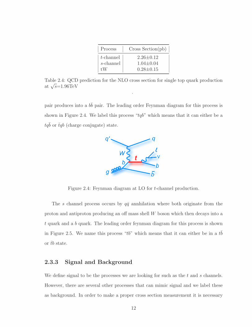
Process Cross Section(pb)
t-channel 2.26±0.12s-channel 1.04±0.04tW 0.28±0.15
Table 2.4: QCD prediction for the NLO cross section for single top quark productionat
√s=1.96TeV
.
pair produces into a bb pair. The leading order Feynman diagram for this process is
shown in Figure 2.4. We label this process “tqb” which means that it can either be a
tqb or tqb (charge conjugate) state.
Figure 2.4: Feynman diagram at LO for t-channel production.
The s channel process occurs by qq annhilation where both originate from the
proton and antiproton producing an off mass shell W boson which then decays into a
t quark and a b quark. The leading order feynman diagram for this process is shown
in Figure 2.5. We name this process “tb” which means that it can either be in a tb
or tb state.
2.3.3 Signal and Background
We define signal to be the processes we are looking for such as the t and s channels.
However, there are several other processes that can mimic signal and we label these
as background. In order to make a proper cross section measurement it is necessary
12

Figure 2.5: Feynman diagram at LO for s-channel production.
to be able to discriminate between the two. If we look back to Figures 2.4 and 2.5 we
can see the decay products for the two signal channels. What we are looking for when
these events occur are the following: One isolated lepton (e or µ) with high pT , large
/ET in the form of a neutrino, 1-2 b-tagged jets and 1-3 light quark jets both with
high pT . We also need to consider that some jets come from the remaining quarks
in the proton and antiproton. This will be discussed in more detail in the selection
chapter (Chapter 5).
The background processes that can mimic single top production are: W+jets,
Z+jets, tt, QCD and Diboson production. The feynman diagrams for each of these
processes are shown in Figure 5.1. The following list summarizes how each of the
background processes can mimic a single top signal:
• Two jets which are close together can be merged into a single jet leading to a
lower jet multiplicity,
• A lepton can be misidentified as a jet and vice versa,
• Jets can be mistagged as b jets when they are not,
• A second lepton in the event (e or µ) may not be detected leading to a fake /ET .
Also some of the jet energies may be misreconstructed which can also lead to a
13

fake /ET .
As an example consider the QCD process in Figure 5.1 (bottom). This is an all jet final
state. However if one of the jets fakes the lepton signature, another is misidentified
by the b-tagging algorithm and the remaining jets energy is not fully measured, then
the resulting signature is one lepton, /ET , and two jets. This would pass the event
selection for a single top event.
2.3.4 CKM Matrix Element |Vtb|
CKM stands for Cabibbo-Kobayashi-Maskawa, which are the last names of the physi-
cists that created the CKM matrix. Nicola Cabibbo initially introduced (1963) a
matrix that described the probability that d and s quarks would decay to u quarks
through the weak interaction. In 1974 the Charm quark was observed and this matrix
became a 2×2 matrix. Kobayashi and Maskawa later came along and realized that
another quark generation needed to be added to explain CP violation because the
two generation of quarks did not do the job. The CKM matrix then became a 3×3
matrix which can be seen below.
d′
s′
b′
=
Vud Vus Vub
Vcd Vcs Vcb
Vtd Vts Vtb
d
s
b
(2.1)
Each of the CKM elements when squared (|Vxy|2) denote the probability that quark
x decay to quark y. If the CKM matrix assumes unitarity and only three quark
generations then we get the following relation:
|Vub|2 + |Vcb|2 + |Vtb|2 = 1. (2.2)
14
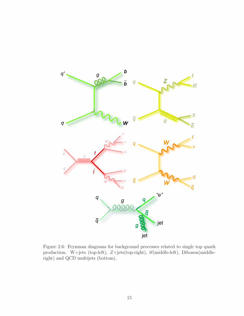
Figure 2.6: Feynman diagrams for background processes related to single top quarkproduction. W+jets (top-left), Z+jets(top-right), tt(middle-left), Diboson(middle-right) and QCD multijets (bottom).
15
Here, the first two components (|Vub| and |Vcb|) have been measured very accurat-
ley [1] which leads to a value for |Vtb|. However, |Vtb|2 is also directly proportional to
the single top quark cross section. Thus a measurement of the singletop cross section
allows us to measure |Vtb| without imposing the three generations and unitarity con-
straint. The relationship between the Wtb vertex and the matrix elemnet |Vtb| can
be seen through the following factor:
− igw
2√2Vtbγ
µ(1− γ5). (2.3)
This thesis presents a measurement of |Vtb| which can be seen in Section 8.4.
2.3.5 Polarization
As stated earlier, the lifetime of the top quark is ∼ 5× 10⁻²⁶s and because of this the
top quark does not fragment. A consequence of this is that all of its spin information
is transmitted to its decay particles (W and b). In the SM the weak interactions are
left handed which means that single top quarks come in a polarized state. The W
helicity (spin + polorization) is then transffered directly to the top decay products
which can be measured. The angles with which the decay products form relative to
the top quark can also be used to identify single top quark production. Studies on
polarization and angular correlations of the top quark can be see in the following
references [12, 13, 14]. These measured properties also add to the validation of the
SM.
2.3.6 Beyond The Standard Model
We briefly talked about one BSM search in Section 2.3.4 (the existence of more than
three generations of quarks). Lets discuss a few more that have a direct connection to
16
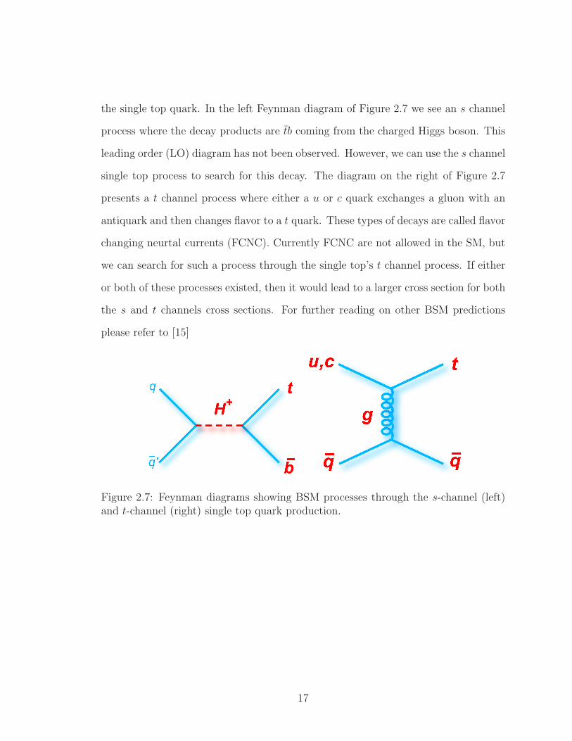
the single top quark. In the left Feynman diagram of Figure 2.7 we see an s channel
process where the decay products are tb coming from the charged Higgs boson. This
leading order (LO) diagram has not been observed. However, we can use the s channel
single top process to search for this decay. The diagram on the right of Figure 2.7
presents a t channel process where either a u or c quark exchanges a gluon with an
antiquark and then changes flavor to a t quark. These types of decays are called flavor
changing neurtal currents (FCNC). Currently FCNC are not allowed in the SM, but
we can search for such a process through the single top’s t channel process. If either
or both of these processes existed, then it would lead to a larger cross section for both
the s and t channels cross sections. For further reading on other BSM predictions
please refer to [15]
Figure 2.7: Feynman diagrams showing BSM processes through the s-channel (left)and t-channel (right) single top quark production.
17
Chapter 3
Accelerators and Detectors
3.1 Introduction
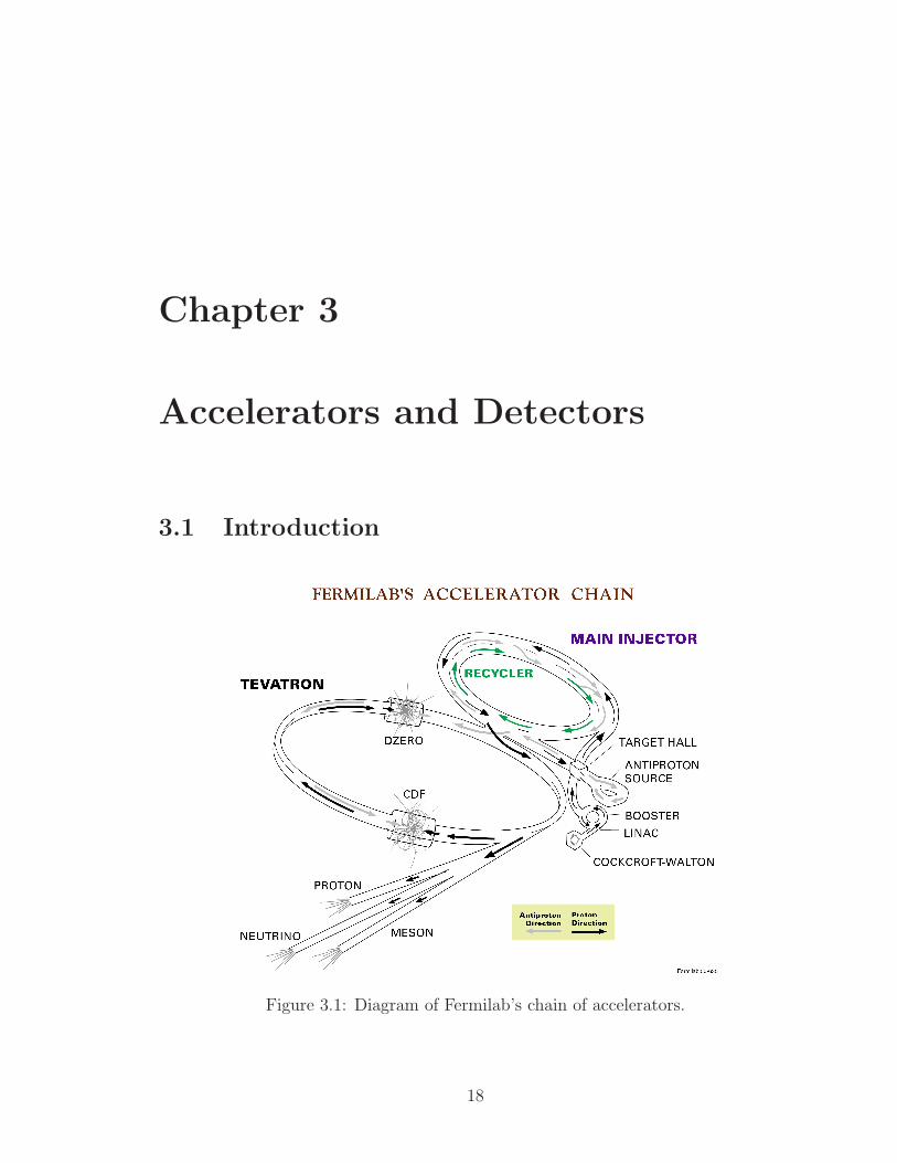
Figure 3.1: Diagram of Fermilab’s chain of accelerators.
18

The Tevatron at Fermilab is the second largest synchrotron in the world. It
accelerates protons and antiprotons up to ∼1 TeV each and collides them at two
detector sites (DØ and CDF) located on opposite sides of the Tevatron ring. The
resulting collisions occur at a center of mass energy of 1.96 TeV. The collision produces
all SM particles excluding the Higgs boson. This chapter discusses the acceleration
sequence used to reach collisions at this energy. This thesis is based on data taken
from the detector site DØ.
In order to get a collision to occur at the center of either the DØ or CDF detectors
we must first understand how the whole process unfolds. The following sections
describe the chain of accelerators and storage rings used to produce pp collisions.
3.2 Cockroft-Walton Pre-accelerator
The first stage of acceleration begins with the Cockroft-Walton pre-accelerator. This
consists of a dome which is mounted on three or four legs as there are two, however
only one is used during acceleration. The legs act as a voltage multiplier (Figure 3.2).
The multiplier takes low voltage AC power input (75 kV) and through the use of
capacitors and diodes steps up the voltage to a provide a DC output voltage of
750 kV. Located within the dome is a bottle of hydrogen gas (H2) and a magnetron.
The Hydrogen molecules get pumped into the magnetron which converts the gas to
H− ions (Figure 3.3). The hydrogen ions (H−) are extracted by an extractor electrode
and accelerated to 750 KeV through a tunnel which is connected to the dome and
grounded at the wall. The H− ions are then transferred to the “750 KeV line” which
has an electrostatic chopper that chops the beam into bunches (40µs each) before
they enter the Linac.
19
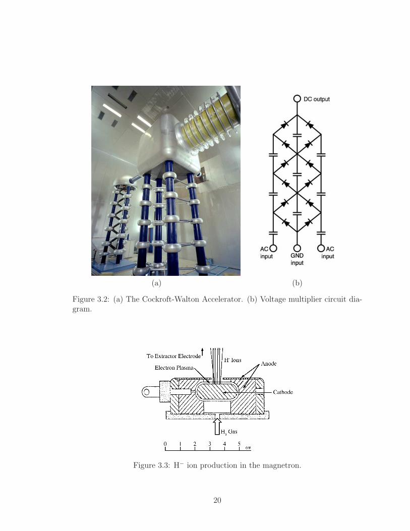
(a) (b)
Figure 3.2: (a) The Cockroft-Walton Accelerator. (b) Voltage multiplier circuit dia-gram.
Figure 3.3: H− ion production in the magnetron.
20

3.3 Linear Accelerator (Linac)
The Linac is divided into two parts, low energy drift tubes (DTL) and the high energy
side coupled (SCL) linacs [16]. The DTL is 79 m long and consists of five tanks, each
powered by a 5 MW amplifier which produces a 201 MHz RF signal. The DTL
accelerates the H− ion bunches from 750 KeV to 116 MeV. The SCL is 67 m long and
consists of seven modules each powered by a 12 MW Klystron amplifier which creates
a 805 MHz RF signal. This section takes the 116 MeV ion bunches and accelrates
them to 400 MeV. The 400 MeV ion bunches from the Linac are sent to the Proton
Booster ring for further acceleration.
3.4 Proton Booster Ring
This is the first synchrotron in the acceleration process [17]. It is a 75 m radius
ring that uses 19 RF cavities to accelerate the beam from 400 MeV to 8 GeV. As
the energy is increased the magnet current is synchronously increased to keep the
beam on a circular orbit. At injection the 400 MeV ion bunches are passed through
a carbon foil, which is used to strip off the electrons leaving only the protons to
accelerate around the synchrotron. Once enough protons are accumulated at 8 GeV
they are transferred to the Main Injector.
3.5 Fermilab Main Injector
The Main Injector is also a synchrotron and has a radius of ∼528 m. The main
injector is a very versatile accelerator that has many “Modes of Operation” [18]. One
of the main modes performs the acceleration of both protons and antiprotons from 8
GeV to 150 GeV for injection into the Tevatron. For protons this is quite easy since
21

they are coming from the Booster. However, for antiprotons the process is involved
as we first have to produce them. This defines a second mode of operation in which
protons are accelerated from 8 GeV to 120 GeV and then sent to the antiproton
source where they are used to produce antiprotons. The next section will cover the
production of antiprotons.
3.6 Antiproton Production
Antiprotons are created by colliding 120 GeV protons from the Main Injector with a
Nickel-Iron alloy target. This produces a jet of particles, some of which are antipro-
tons. A Lithium collection lens is then used to focus the negatively charged particles
using a pulesed magnetic field. This is followed by a magnet which is used to mo-
mentum select the antiprotons that have an energy of about 8 GeV. Antiprotons are
produced every 2.4 seconds through this process. A diagram of this process can be
seen in Figure 3.4. The antiprotons are then transferred to the debuncher.
The Debuncher is a synchrotron that takes the shape of a rounded triangle with
an average radius of 90 m. It is used to reduce the transverse momentum spread of
the beam through stochastic cooling [19] and debunches the beam by using RF kicks
to produce a continous antiproton beam. The debuncher does no acceleration and it
maintains the beam energy of 8 GeV.
From the debuncher the beam is transferred to the antiproton accumulator. This
is very similar to the debuncher and resides in the same tunnel. It has an average
radius of 75 m and is used to further cool the beam. Unlike the debuncher the beam
stays in the accumulator for several hours and it is rebunched before being extracted
to the last element of the antiproton production complex, the recycler.
The Recycler is a storage ring which resides just above the Main Injector. It is
22

Figure 3.4: Schematic diagram of the Target and Lens system. [19].
used for the third phase of the beam cooling. It uses both stochastic and electron
cooling [20]. Once the Recycler is sufficiently filled with antiprotons the 8 GeV beam
is sent to the Main Injector for acceleration to 150 GeV.
3.7 Tevatron
Once there is a sufficient number of antiprotons the Main Injector injects the 150 GeV
proton beam into the Tevatron in 36 bunches where each bunch is separated by 396 ns.
In addition, after every 12th bunch there is an additional 2.64 µs separation. Once the
protons are loaded then the same thing is done with the antiprotons, the combined
operation is referred to as a “store”. The Tevatron is the last synchrotron is the
acceleration process. It is a ∼4 mile ring which accelrates the beams from 150 GeV
to 980 GeV each. It uses superconducting magnets and RF cavities to steer and
accelerate the beams. The protons and antiprotons travel in opposite directions in
23
the same tunnel by rotating around one another in a helical path. At two loactions
there are two detectors (DØ and CDF) where the beams are brought into collision.
This gives pp collisions with a center of mass energy of 1.96 TeV.
3.8 DØ Detector
The initial design for the DØ detector was the merger of two somewhat different
proposals, a non magnetic detector with precision calorimetry and a detector with
extensive muon detection over a large range of rapidity. This is the basis of the
Run I DØ detector which was operated from 1992 until 1996 [22]. Between 1996
and the start of Run II in 2001, the detector was upgraded with the addition of
a central magnetic field, a new central tracking system and a new forward muon
spectrometer [23]. The present detector has four main detection systems: a central
tracking system, a preshower system, central and forward calorimeters and central and
forward muon spectrometers. Each of the sub-systems is described in the following
sections.
3.8.1 DØ Coordinate System
DØ uses a right-handed coordinate system centered at the middle of the DØ detector.
The z-axis points along the path of the proton, the x-axis points outward along the
radius of the Tevatron and the y-axis points upward (Figure 3.6). Thus the position
of a particle originating from a collision at x = y = z = 0 can be defined in terms of
its distance from the origin, r =√
x2 + y2, and two angles θ and φ. θ is defined as
the polar angle with respect to +z-axis and φ is the azimuthal anlgle, defined with
respect to the +x-axis. Rather than using θ, it is often more convenient to use the
24
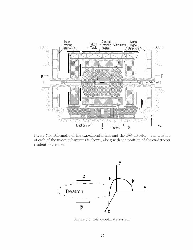
Figure 3.5: Schematic of the experimental hall and the DØ detector. The locationof each of the major subsystems is shown, along with the position of the on-detectorreadout electronics.
Figure 3.6: DØ coordinate system.
25
pseudorapity, η, which is defined by:
η ≡ − ln
(
tanθ
2
)
. (3.1)
This is an approximation of the true rapidity, y, in the relativistic limit m << E,
which is valid in almost all of the cases considered here. The rapidity of a particle is
Lorentz invariant and is given by:
y =1
2ln
(
E + pzE − pz
)
, (3.2)
The psedorapidity is approximately Lorentz invariant and is more convenient variable
than y, because the particle density per unit η is much more uniform than that of y.
In practice there is a finite spread in the z-position of the collision point, so that
collisions often do not occur exactly at x = y = z = 0. In this case the pseudorapidity
is defined with respect to the collision vertex.
3.8.2 Central Tracking System
Charged particle detection and measurement is performed by the central tracking
system. For DØ this has two components, the silicon microstrip tracker (SMT) and
the central fiber tracker (CFT). The trackers are located inside of a solenoidal magnet
which produces a 2 Tesla magnetic field (Figure 3.7). The combined tracker-magnet
system is used to locate and identify particles and measure their momentum. It
also locates the position of the collision or primary interaction. The SMT and CFT
trackers loacte the position of particles as they pass through them and the bend of
the track in the magnetic field provides a measurement of the particle momentum.
Once this is done we can then use sophisticated algorithms to identify and trace back
26
the particles point of origin.
Figure 3.7: Schematic of the central tracking showing the location of SMT and CFTcomponents with respect to the beam axis.
The SMT is used as the first line of detection and is therefore positioned at the
center of the DØ detector. As shown in Figure 3.8, it is comprised of six barrel
sections, and sixteen transversly mounted disks. The barrel sections provide mea-
surement of the coordinates r and φ and the disks measure the coordinates r, z and
φ. The detector elements are formed from silicon wafers with readout strips etched
onto either one or both sides of the wafer. Charged particles passing through the
bulk of the silicon create electron-hole pairs which result in an induced pulse in the
strips on the wafer surfaces. The strips on the top an bottom surfaces have a finite
crossing angle, thereby providing a spatial measurement of the track position. The
SMT covers the pseudorapidity range |η| < 3.8.
The CFT detector is composed of eight concentric cylinders which surround the
27
1.2 m
Figure 3.8: The elements of the SMT detector, showing the barrel and disc segmen-tation.
SMT. It has a regional coverage of r = 20-52 cm and |η| = 1.7. Eeach cylinder consists
of two doublet layers of scintillating fibers. The first layer lies along the z-axis and
the second has a stereo angle of φ = ±3◦ relative to the z-axis. The scintillating
fiber, when excited by a charged particle, gives off light which then travels down a
wave guide to be readout by a visible light photon counter (VLPC). The CFT has a
resolution of 100 µm.
The DØ solenoid is a superconducting magnet made from niobium-titanium wire
which carries a current of 4.7 kA and produces a 2 T magnetic field that lies parallel to
the z-axis. The magnet is used to bend charged partiles so that their momentum can
be measured from the track curvature. In the transverse plane, this can be expressed
in the form:
pT = 0.3qBr. (3.3)
Where, q is the charge of the particle, B is the strength of the magnetic field and r is
the radius of curvature. A schematic of the solenoid and the muon toroid magnets is
shown in Figure 3.9, together with a representation of the the resulting field pattern
inside of the detector.
The preshower detector is broken into two parts, the central preshower detec-
tor (CPS) and the forward preshower detector (FPS). These are located between the
28

Figure 3.9: Schematic representation of theDØmagnets and the magnetic field withinthe detector volume.
29

solenoid and the calorimeters. The CPS has a regional coverage of |η| < 1.3 at a
radius of 72 cm and the FPS covers 1.5 < |η| < 2.5. The CPS is composed of a lead
radiator followed by three layers of scintillating fibers. The FPS consists of two layers
of scintillating fibers, a lead radiator then another two layers of scintillating fibers.
The location of the detectors is shown in Figure 3.7. The preshower detector helps
in the identification of electrons and photons which begin to shower when hitting the
radiator. It also aids in the identification of heavier particles which will leave only
single tracks.
3.8.3 DØ Calorimeters
Figure 3.10: Schematic diagram shown the DØ central endcap calorimeters. The cutaway shows the details of the calorimeter modules [26].
The DØ calorimetry is divided into three sections, the central module (CC) and
the two endcap modules (ECN, ECS) (Figure 3.10). It is designed to measure the en-
30
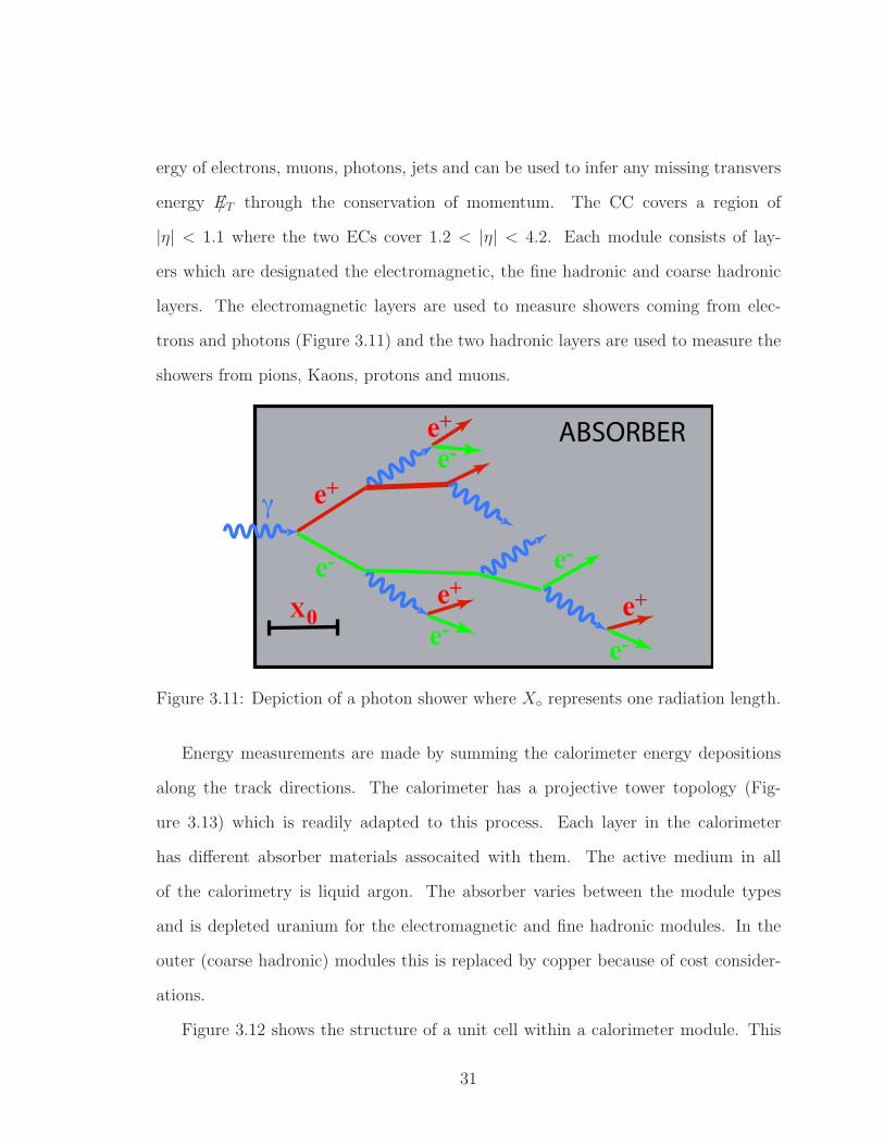
ergy of electrons, muons, photons, jets and can be used to infer any missing transvers
energy /ET through the conservation of momentum. The CC covers a region of
|η| < 1.1 where the two ECs cover 1.2 < |η| < 4.2. Each module consists of lay-
ers which are designated the electromagnetic, the fine hadronic and coarse hadronic
layers. The electromagnetic layers are used to measure showers coming from elec-
trons and photons (Figure 3.11) and the two hadronic layers are used to measure the
showers from pions, Kaons, protons and muons.
Figure 3.11: Depiction of a photon shower where X◦ represents one radiation length.
Energy measurements are made by summing the calorimeter energy depositions
along the track directions. The calorimeter has a projective tower topology (Fig-
ure 3.13) which is readily adapted to this process. Each layer in the calorimeter
has different absorber materials assocaited with them. The active medium in all
of the calorimetry is liquid argon. The absorber varies between the module types
and is depleted uranium for the electromagnetic and fine hadronic modules. In the
outer (coarse hadronic) modules this is replaced by copper because of cost consider-
ations.
Figure 3.12 shows the structure of a unit cell within a calorimeter module. This
31
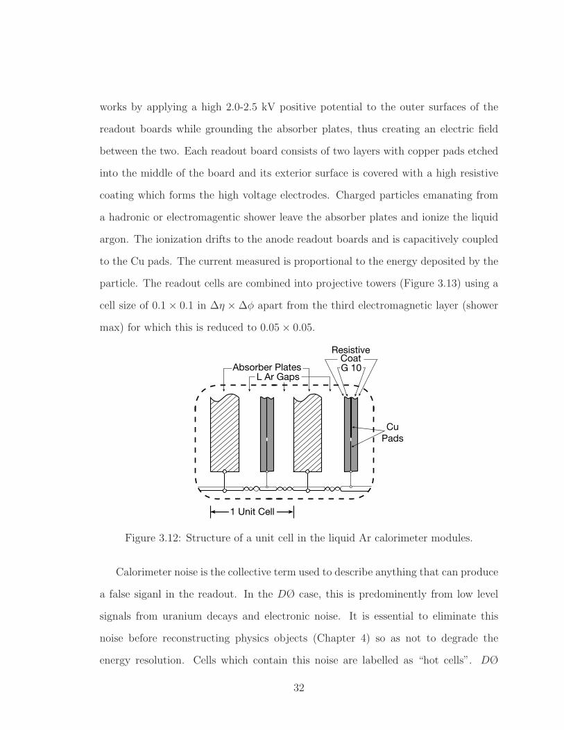
works by applying a high 2.0-2.5 kV positive potential to the outer surfaces of the
readout boards while grounding the absorber plates, thus creating an electric field
between the two. Each readout board consists of two layers with copper pads etched
into the middle of the board and its exterior surface is covered with a high resistive
coating which forms the high voltage electrodes. Charged particles emanating from
a hadronic or electromagentic shower leave the absorber plates and ionize the liquid
argon. The ionization drifts to the anode readout boards and is capacitively coupled
to the Cu pads. The current measured is proportional to the energy deposited by the
particle. The readout cells are combined into projective towers (Figure 3.13) using a
cell size of 0.1 × 0.1 in ∆η ×∆φ apart from the third electromagnetic layer (shower
max) for which this is reduced to 0.05× 0.05.
Figure 3.12: Structure of a unit cell in the liquid Ar calorimeter modules.
Calorimeter noise is the collective term used to describe anything that can produce
a false siganl in the readout. In the DØ case, this is predominently from low level
signals from uranium decays and electronic noise. It is essential to eliminate this
noise before reconstructing physics objects (Chapter 4) so as not to degrade the
energy resolution. Cells which contain this noise are labelled as “hot cells”. DØ
32
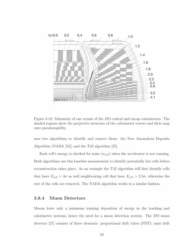
Figure 3.13: Schematic of one octant of the DØ central and encap calorimeters. Theshaded regions show the projective structure of the calorimeter towers and their maponto pseudorapidity.
uses two algorithms to identify and remove them: the New Anomalous Deposits
Algorithm (NADA [24]) and the T42 algorithm [25].
Each cell’s energy is checked for noise (σcell) when the accelerator is not running.
Both algorithms use this baseline measurement to identify potentially hot cells before
reconstruction takes place. As an example the T42 algorithm will first identify cells
that have Ecell > 4σ as well neighbouring cell that have Ecell > 2.5σ, otherwise the
rest of the cells are removed. The NADA algorithm works in a similar fashion.
3.8.4 Muon Detectors
Muons leave only a minimum ionizing deposition of energy in the tracking and
calorimeter systems, hence the need for a muon detection system. The DØ muon
detector [27] consists of three elements: proportional drift tubes (PDT); mini drift
33

tubes (MDT); an array of scintillation counters and three 1.8 T toroidal magnets.
The central part of the muon system covers the region |η| < 1 and the forward part
covers 1 < |η| < 2. The muon spectrometer is divided into the A, B and C layers
where the toroidal magnets lie between layers A and B. An expanded view of the
chambers and scintillation counters is shown in Figure 3.14.
The PDTs and MDTs measure the position and momentum of the muons passing
through them, with the PDTs in the barrel (central) part of the detector, and the
MDTs the forward regions. Both types of drift tubes have a similar construction.
The two sides of each drift tube have a negative voltage applied to them, while the
wire running down the middle of the tube that has a positive voltage. The drift tubes
are filled with a inert gas mixture that gets ionized when muons pass through. The
electrons that drift toward the anode wire and produce a signal pulse on the wire.
The ionization takes a finite (drift) time to reach the anode. For the PDTs, this is
500 ns, and for the MDTs it is 100 ns. The scintillation counters work much the same
way as the scintillating fibers and have a response time of 1.6 ns that allows for precise
timing measurements. Because of this they are able to correlate muon hits with bunch
crossings and can also determine if a muon came from a pp collision or from outside
of the detector (Cosmic ray Muons). The toridal magnets are used to bend muons in
the 1.8 T field which allows for more precise measurements of momentum.
3.8.5 Luminosity Monitor
The DØ luminosity monitors (LM) consists of two circular detectors made of 24
scintillating tiles each. The detectors are located at ±144 cm along the z-axis and
has a regional coverage of 2.7 < |η| < 4.4 (Figure 3.15). The luminosity is measured
34

Figure 3.14: Exploded view of the DØ muon detection system. The top diagramshows the the configuration of the A, B and C layers in the barrel and forwardregions. The bottom diagram shows the location of the barrel and forward scintillationcounters.
35

by the following equation:
L =fNLM
σLM
. (3.4)
Where, f is the frequency of the crossing beam, NLM is the average number of in-
elastic collisions and σLM is the effective cross section [26]. The LM is also used to
discriminate between pp interactions and the beam and it can also be used to make
a quick measurement of the position of the interaction vertex along the z-axis.
Figure 3.15: Diagram of the Luminosity monitors at DØ [26].
3.9 Trigger Framework
The job of the trigger framework is set up to analyze the data coming from all the
detection systems that comprise the DØ detector and decide which of the events
should be recorded for analysis. The raw event rate of 1.7 MHz would result in the
need to record more than one petabyte of data per second, which is far too large
to handle. The practical limit is a trigger rate of ∼100 Hz for recording to tape,
requiring a rate reduction of ∼ 2× 10⁴. This is done using the three trigger level DØ
framework (Figure 3.16).
The lowest level trigger (L1) consists of firmware and hardware and reduces the
event rate of 1.7 MHz to 2 KHz. This needs to make decisions very quickly (3.5 µs)
36
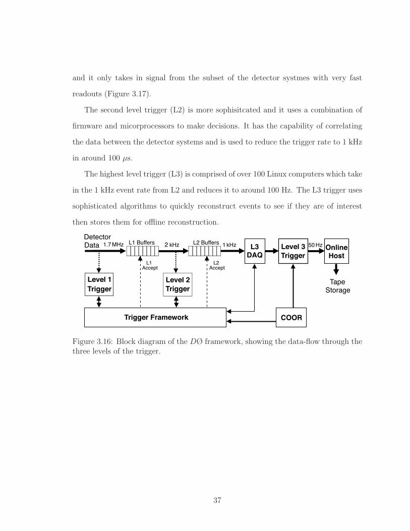
and it only takes in signal from the subset of the detector systmes with very fast
readouts (Figure 3.17).
The second level trigger (L2) is more sophisitcated and it uses a combination of
firmware and micorprocessors to make decisions. It has the capability of correlating
the data between the detector systems and is used to reduce the trigger rate to 1 kHz
in around 100 µs.
The highest level trigger (L3) is comprised of over 100 Linux computers which take
in the 1 kHz event rate from L2 and reduces it to around 100 Hz. The L3 trigger uses
sophisticated algorithms to quickly reconstruct events to see if they are of interest
then stores them for offline reconstruction.
Figure 3.16: Block diagram of the DØ framework, showing the data-flow through thethree levels of the trigger.
37
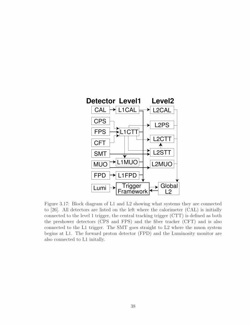
Figure 3.17: Block diagram of L1 and L2 showing what systems they are connectedto [26]. All detectors are listed on the left where the calorimeter (CAL) is initiallyconnected to the level 1 trigger, the central tracking trigger (CTT) is defined as boththe preshower detectors (CPS and FPS) and the fiber tracker (CFT) and is alsoconnected to the L1 trigger. The SMT goes straight to L2 where the muon systembegins at L1. The forward proton detector (FPD) and the Luminosity monitor arealso connected to L1 initally.
38

Chapter 4
Event Reconstruction
When a pp inelastic collision occurs at DØ there are many particles produced that
travel through the detector and are measured by the tracking system and the calorime-
ters. It is the job of the reconstruction code to convert the raw signals (pulse-heights
and positions) into reconstructed charged and neutral particles. These in turn are
grouped into jets and projected to their point of origin, to define production vertices.
For this analysis, the principal objects of interest are electrons, muons, jets (light and
heavy quark), the position of primary and secondary vertices, and the missing en-
ergy ( /ET ). To reconstruct and identify physics objects there are ceartin requirements
that must be followed, which are discussed in the following sections.
4.1 Charged Track Reconstruction
When charged particles traverse the SMT and CFT they deposit only a small amount
of energy via dEdx
and their presence is identified by a pulse or hit in a specific part of
the detector readout. The reconstruction code takes these hits and builds them in to
tracks eminating from a vertex or point of production for a particular event. Since
39

both the SMT and CFT are inside a strong magnetic field the extrapolated tracks are
curved. For any particular hard interaction there will be many hits corresponding to
many tracks making the process of track finding complicated. In order to solve this
problem DØ uses two different algorithms to define tracks. These are the histogram
track finding (HTF) [28] and the alternative AA [29] algorithms. To define the final
set of tracks in an event these algorithms are combined using global track reconstruc-
tion (GTR). GTR relies on a Kalman Filter algorithm [30] which cleans and smooths
the tracks before they are stored for analysis.
The HTF method [28] uses all possible hits in (x, y) space and maps them to
points in (ρ, φ) space while taking account of the point of interaction. Here, ρ is the
curvature of the track and φ is the direction of the track. Using these two parameters
2D histograms are built allowing the identification of tracks. If there is a particle
corresponding to a collection of hits in the tracking volume then those hits should all
have the same curvature and direction. These appear as peaks in the 2D histograms
thus allowing the identification of tracks. In contrast, the hits associated with other
tracks will be spread uniformly throughout the hitogram. For a detailed description
of the algorithm please see Ref. [28].
The AA algorithm [29] begins with a hypothesis that a track must have at least
three hits in the SMT in order to be reconstructed. All three hits must occur in
succession where the first hit can be in either an SMT barrel or F-disk. The second
hit must form an angle with the first hit and relative to the beam spot where ∆φ <
0.08 (Figure 4.1). The third hit is required to have a “radiusMin” > 30 cm and an
“impactMax” < 2.5 cm (Figure 4.1), where radiusMin is the radius of curvature of the
track and impactMax is the axial impact parameter with respect to x = y = z = 0.
Also, all three hits are required to have a fit of χ2 < 16. If all these requirements are
met the algorithm extrapolates outwards to the following tracking layers searching for
40

Figure 4.1: Diagram of track reconstruction using the AA algorithm.
more hits assocaiated with that track. As the number of hits grows the track fit is still
required to have a χ2 < 16. If there are many hits on one layer then the algorithm
creates a new hypothesis. The whole process continues until the detector ends or
three successive layers are missed. For a detailed discussion please see Ref. [29].
Tracks from both the HTF and AA are then analyzed using global track recon-
struction (GTR). GTR uses a Kalman Filter to refit, clean and smooth the tracks
resulting in a final set of tracks.
4.2 Primary Vertex
The primary vertex is defined as the location of the hard inelastic collision between the
proton and antiproton. The process of locating the interaction point is complicated
by the presence of secondary vertices, such as those from b quark decays, and the
41

presence of multiple interactions when running at high luminosity.
To deal with these complications DØ uses an adaptive primary vertex algo-
rithm [31] to identify the position of the primary vertex. This is done in three steps:
track selection, vertex fitting, and vertex selection.
Tracks are selected by requiring at least two hits in the SMT and a pT > 0.5. The
selected tracks are then clustered relative to the z-axis and must be within 2 cm of
each other in z. Vertex fitting then uses a 2-pass process, where the first pass fits
the clustered tracks to a common vertex , and the second pass chooses the clusters
that are consistent with the position of the beam spot. The clustering is done using
a Kalman Filter which removes tracks with a high χ2 until a χ2/ndf < 10 is achieved
for the cluster. In the second pass only the clusters which lie within 5σ of beam spot
are retained. Lastly, the primary vertex is chosen from the remaining candidates by
selecting the vertex which has the minimum probability of being a minimum bias
interaction [32].
4.3 Electron Identification
The signature of an electron in the DØ detector is a track in the central tracker
which matches to an electromagnetic shower in calorimeters. Electromagnetic cluster
candidates are identified from the energy deposited in the calorimeter towers using a
basic cone algorithm [33] with the requirement that almost all of the energy is found
in the EM calorimeter. To be considered an electron candidate, a cluster must have
a track from the central tracker which spatially matches to the cluster. The criteria
used for both steps are discussed below.
Cluster candidates are identified using three criteria for the energy profile within
the calorimeter. These are the cluster electromagnetic fraction, fEM , its isolation,
42

fiso, and its H-matrix χ2, χ2H . These are defined below. The EM fraction is defined
by:
fEM =EEM
Etotal
. (4.1)
Where, EEM is the amount of electromagnetic energy in the cluster and Etotal is the
total cluster energy. A cone size ∆R = 0.2, where ∆R =√
∆η2 +∆φ2, is used
for energy clustering and clusters are only retained if they have an electromagnetic
fraction, fEM > 0.9. The next step is the cluster isolation requirement, which is
defined using the equation:
fiso =Etotal(R < 0.4)− EEM(R < 0.2)
EEM(R < 0.2). (4.2)
Where, Etotal(R < 0.4) is the energy observed in a cone of size ∆R = 0.4, centered on
the electromagnetic cluster and EEM(R < 0.2) is the cluster energy. For an isolated
electron, fiso should peak close to zero. The requirements used in this analysis are
listed in Table 4.1, below.
The last requirement for the cluster selection is a cut on transverse and depth
profiles of the electromagnetic shower in the calorimeter. This is done using the
H-matrix χ2, χ2H [34], which compares the observed profiles to those expected for
an electron on the same energy. This uses seven shower shape variables to define
a 7 × 7 covariace matrix. The matrix is then used to calculate a χ2H by comparing
the observed and predicted energy depositions. The seven inputs to χ2H are: the
fractions of the energy in each of the four layers of the electromagnetic calorimeter,
the transverse width of the shower in the fourth layer (position of shower max),
log10(EEM) and the z position of the primary vertex. To be retained, a cluster is
required to have χ2H < 50.
43
At this point, the cluster list contains both electron and photon candidates. The
last part of the selection is to require a match between the cluster and a track from the
central tracker. This is done using a cut on the probability of the matching χ2, P (χ2).
This contains contribution from both the spatial matching and the energy-momentum
matching between the cluster and the track.
An important factor for this analysis is the ability to simulate the background
from QCD events in which the electron signature is faked due to jet fluctuations
or charge/neutral pion overlaps. As this is very difficult to simulate reliably with
a monte carlo, this is done using a subset of the data. For this we define one last
measure of electron quality, the electron likelihood,
Le(~x) =PS(~x)
PS(~x) + PB(~x), (4.3)
where the vector ~x has seven dimensions and the subscripts S and B denote signal
(genuine electrons) and background (fake electrons). The dimension of x are: fEM ,
P (χ2spatialmatch), track-cluster
Epratio, χ2
H , track distance of closest approach to the
primary vertex, Σ∆R = 0.4 (track pT ), Σ∆R = 0.05 (no tracks) [35]. The cones for the
last two of these are defined with respect to the cluster axis. For the purpose of later
clarity it is convenient at this point to define three classes of electron candidates,
which are denoted ultraloose, loose and tight. The ultraloose category is used to
define the misidentification background from QCD and the loose and tight categories
are used in the selection of signal events (see later). These are defined in Table 4.1
below.
44

Quantity Ultraloose Loose Tight
fEM > 0.9 > 0.9 > 0.9χ2H < 50 < 50 < 50
fiso < 0.2 < 0.2 < 0.2pT > 15 GeV > 15 GeV > 15 GeVP (χ2) NA > 0 > 0Track match pT NA > 5 GeV > 5 GeVTracks match with PV NA ∆z < 1 CM ∆z < 1 CMLe NA NA > 0.85
Table 4.1: Definitions for three classes of electron candidates.
4.4 Muon Reconstruction
If a muon track has a momentum ≥ 3.5 GeV , it will be seen by the tracking system,
the calorimeters and the muon detectors. In this analysis, muon candidates are
required to have hits in all three layers of the muon system. The B and C layer
chambers see no magnetic field so that the BC segment of the track is found as a
straight line. To define a muon track candidate, the extrapolation of a segment found
in the B and C layers is required to match to a segment in the A layer chambers and
to a track in the central tracker. For this analysis two categories of muon candidates
are used. These are based on the extent to which the track is isolated and both are
used in the selection of signal events (see later).
Loosely isolated muons candidates are required to have at least two hits in both
the A layer and combined B+C layer chambers. To reject the background from cosmic
ray muons, candidates are also required to have hits in the A and B+C layer muon
scintillators which are within 10 ns of the bunch crossing time. They must also have
a match to a track in the central tracker with a χ2 < 4 if the track has a dca < 0.2 cm
with respect to the primary vertex or a dca < 0.02 cm for hits in the SMT. To
be retained for further analysis, muon candidates must have pT > 4 GeV and have
45
∆R (µ, nearest jet) > 0.5.
A second category, designated as tightly isolated muons, must satisfy the loose
isolation requirements and cuts on two additional quantities which look at the pT -
normalized energy and momentum flow about the muon track. These are the scaled
track halo [36] and the scaled calorimeter halo [36] cuts, which are defined as:
ScaledTrackHalo = |∑
Tracks
pTpT (µ)
|, for,∆R(track,muontrack) < 0.5, (4.4)
ScaledCalorimeterHalo = |∑
cells
ET
pT (µ)|, for, 0.1 < ∆R(cells,muoncal-track) < 0.4.
(4.5)
In equation 4.4 the requirment is that the total transverse momentum of tracks sur-
rounding the muon track in a cone of ∆R < 0.5 must be less than 20% of the muon
pT . Same idea is used in equation 4.5 however, here the sum of the energy excludes
the region ∆R < 0.1, which is occupied by the muon dEdx
deposition.
4.5 Jet Reconstruction
In a hadron collider, jets are frequently produced and can be defined as an associated
group of particles which come from the hadronization of a quark or gluon. Since a
typical jet contains both charged and neutral particles, full jet reconstruction requires
the information from both the hadronic and electromagnetic calorimeters. This is
done by clustering the energy deposited within a cone in ∆R space. The resulting
clustered energy is then associated with a hadronic jet. This process is discussed in
the follwing paragraphs.
DØ uses the Run II Improved Legacy Cone Algorithm (ILC) [38, 39] for jet
reconstruction. This algorithm is implemented in three steps. The first step takes
46

a number of calorimeter towers with pT > 0.5 GeV and forms pre-clusters. To
accomplish this, the algorithm starts from a pT -ordered list of towers and associates
the towers with pT > 1 MeV that lie within ∆R = 0.3 to form pre-clusters. The
associated towers are then removed from the list and the procedure is repeated until
all of the towers have been pre-clustered.
The next step is to form proto-jets. This starts from a pT -ordered list of the pre-
clusters. Starting from the highest energy pre-cluster, the pre-clusters are associated
within ∆R = 0.5 to form a proto-jet. The jet axis is then re-determined and the
process is iterated until either the jet energy converges or the pT of the jet falls below
4 GeV. All proto-jets with pT < 4 GeV are discarded, as are any pre-clusters that lie
within R = 0.25 of a stable proto-jet. The algorithm iterates the association until all
of the stable proto-jets have been identified.
The final step in the reconstruction process involves the merging and splitting of
prot-jets. Proto-jets which share more than 50% of their energy with another jet are
merged to form a single jet, whereas if the shared fraction is less than 50% the energy
is split to form two jets.
The jets used in this analysis are required to have pT > 15 GeV and to lie within
|η| < 3.4. They are also required to satisfy the quality criteria defined by the DØ
Jet-ID group [40]. These are designed to remove fake jets produced by noise in
the detector modules (hot cells) or problems in the associated electronics. Jets are
removed if more than 90% of their energy is coming from a single calorimeter cell
or the ratio of the most energetic to second most energetic cell is higher than ten.
They are also required to have a coarse hadronic energy fraction of below 44% and an
electromagnetic energy fraction between 5 and 95%. Five of the main requirements
are listed below.
47

Figure 4.2: Schematic of the parton fragmentation process and the particle showeringused to detect the fragmentation products in the calorimeters.
• The EM fraction is required to be 0.05 < fEM < 0.95.
• Jets occuring in the coarse hadronic layers must have a fCH < 0.44 for the CC
region and fCH < 0.46 for the EC.
• If a cell with the most energy has ten times more energy than the second most
energetic cell it is removed where fHOT = Ecell1
Ecell2< 10.
• If 90% of a jets energy is contained in one calorimeter tower it is removed.
4.5.1 Calibration of the Jet Energy Scale
Figure 4.2 shows a schematic of the evolution of a jet from production through to
detection by the calorimeters. Each parton from the hard scattering process undergoes
fragmentation and is detected by the calorimeters as the collection of particle showers,
48

which we have identified as a jet. The jet energy measured by the detector is different
from that of the parent parton because of the complications of the fragmentation
process folded with the effects of finite jet resolution and non-associated backgrounds.
To account for this difference we make corrections to the reconstructed jet in order
to obtain a better estimate of the energy of the parent parton. This is done using the
equation:
Ecorrectedjet =
Euncorrectedjet − Eo
Fη ×R× S, (4.6)
where, Euncorrectedjet is the jet energy measured after reconstruction and Eo is an offset
correction which allows for non-associated background. Fη represents the detector
relative response, R is the response, and S is the showering correction. The role of
these corrections is discussed below.
Eo: The offset correction, Eo, is assocaited with energy reconstructed as part of
the jet that is not coming from the parent parton. This energy comes from electronic
noise, uranium decays, interactions occuring in the same bunch crossing and pile-
up (energy due to other collisions which are not part of the same bunch crossing).
R: The response correction, R, is determined using the Missing ET Projection
Fraction method (MPF). This calculates how how much of the jet energy is not
measured by the detector. This missing energy comes from detector regions that are
not fully instrumented, and the regions of the detector which have a non-uniform
hadronic/electromagnetic energy ratio. This correction is the largest, and accounts
for 30% of the overall correction.
Fη: The relative response correction, Fη, is also determined using the MPF
method. The CC and EC calorimeters are resonably uniform whereas the regions
between the calorimeters (0.5 < |η| < 1.8) are not. Fη is used to correct these non-
uniformities and poorly instrumented regions. It is also used as a function of η to do
49
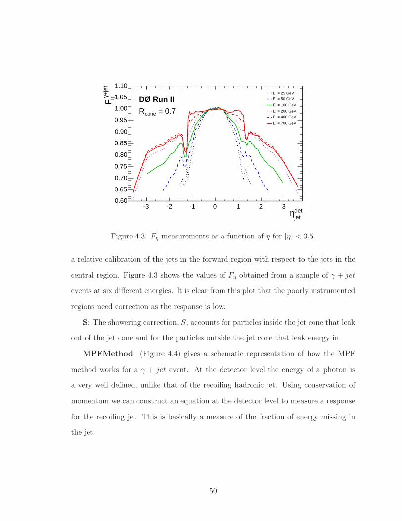
jetdetη
-3 -2 -1 0 1 2 3
η+
jet
γ F
0.60
0.65
0.70
0.75
0.80
0.85
0.90
0.95
1.00
1.05
1.10E’ = 25 GeV
E’ = 50 GeV
E’ = 100 GeV
E’ = 200 GeV
E’ = 400 GeV
E’ = 700 GeV
= 0.7coneR
DØ Run II
Figure 4.3: Fη measurements as a function of η for |η| < 3.5.
a relative calibration of the jets in the forward region with respect to the jets in the
central region. Figure 4.3 shows the values of Fη obtained from a sample of γ + jet
events at six different energies. It is clear from this plot that the poorly instrumented
regions need correction as the response is low.
S: The showering correction, S, accounts for particles inside the jet cone that leak
out of the jet cone and for the particles outside the jet cone that leak energy in.
MPFMethod: (Figure 4.4) gives a schematic representation of how the MPF
method works for a γ + jet event. At the detector level the energy of a photon is
a very well defined, unlike that of the recoiling hadronic jet. Using conservation of
momentum we can construct an equation at the detector level to measure a response
for the recoiling jet. This is basically a measure of the fraction of energy missing in
the jet.
50
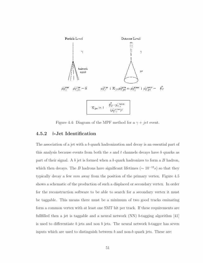
Figure 4.4: Diagram of the MPF method for a γ + jet event.
4.5.2 b-Jet Identification
The association of a jet with a b quark hadronization and decay is an essential part of
this analysis because events from both the s and t channels decays have b quarks as
part of their signal. A b jet is formed when a b quark hadronizes to form a B hadron,
which then decays. The B hadrons have significant lifetimes (∼ 10−12s) so that they
typically decay a few mm away from the position of the primary vertex. Figure 4.5
shows a schematic of the production of such a displaced or secondary vertex. In order
for the reconstruction software to be able to search for a secondary vertex it must
be taggable. This means there must be a minimum of two good tracks eminating
form a common vertex with at least one SMT hit per track. If these requirements are
fullfilled then a jet is taggable and a neural network (NN) b-tagging algorithm [41]
is used to differentiate b jets and non b jets. The neural network b-tagger has seven
inputs which are used to distinguish between b and non-b quark jets. These are:
51

• the significance of the decay length,
• the weighted sum of the track impact parameters,
• the probability that the jet originates from the primary vertex,
• the χ2/ndf of the secondary vertex fit,
• the number of tracks in the secondary vertex,
• the mass of the secondary vertex,
• the number of secondary vertices reconstructed within the jet.
The algorithm outputs a value between 0 and 1 that is associated to the probability
that the jet comes from a b-quark. The choice of a cut value in the network discrimi-
nant defines the operating point for the tagger. For this analysis we use the tight and
loose operating points, for which the discrimenent cuts are set to > 0.775 and 0.5,
respectively. The loose operating point is used for the case where an event is required
to have two b-tagged jets and the tight operating point is used if only one b-tagged
jet is required.
4.6 Reconstruction of Missing Transverse Energy,
/ET
In this analysis neutrinos are part of the signal we are looking for, however they are
not detected at the DØ detector. We can however, infer their transverse momentum
by using the conservation of momentum in the transverse plane. This is a two step
process in which we first form the sum of the calorimeter cell depositions and then
we apply corrections to account for the unmeasured energy due to any muons in the
52
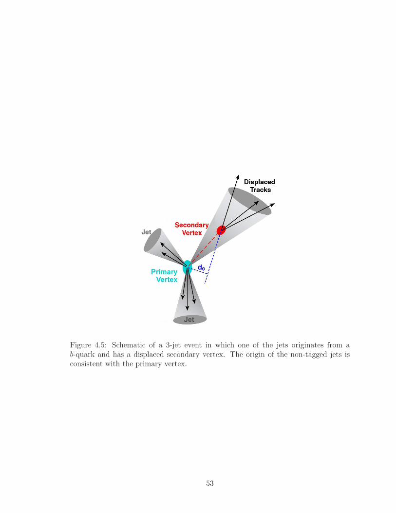
Figure 4.5: Schematic of a 3-jet event in which one of the jets originates from ab-quark and has a displaced secondary vertex. The origin of the non-tagged jets isconsistent with the primary vertex.
53

event. The calorimeter cell sum runs over the cell energies, assuming that they have
a common origin at the primary vertex. This uses the cell 3-momentum, ~p celli for each
of the i electromagnetic and hadronic cells which should vectorially sum to ∼zero if
no neutrinos or muons are present and the detector had a perfect resolution.
/~E uncorrT = −
∑
i
~p celli ; (4.7)
The presence of one or more muons in the event will modify the imbalance and only
a fraction of their momentum (that due to dEdx
in the calorimetry) is included in
the sum. In the second step, this is corrected for by modifying the summation to
include the muon 3-momentum, taken from the tracker, with a small adjustment to
the cell sum for the cells traversed by the muon track. The resolution can be further
improved if the event contains identifiable electrons or photons as their energies are
typically better measured than the simple cell sum would give. This is also covered
in the second level of correction. The best estimate of the transverse energy due to a
neutrino is,
/~E corrT = /~E uncorr
T −∑
objects
(
~p object −∑
i∈object~p celli
)
, (4.8)
where the object sum runs over all of the identified electrons, photons and muons,
~p object is the particle momentum and cell sum runs over all of the cells traversed by
the particle.
54

Chapter 5
Data Samples and Event Selection
After the Data and simulated event samples have been reconstructed we can begin
to use these samples to optimize the event selection. Initially the quality of the data
is checked in order to see if there are any needed corrections. Selection cuts are then
implemented to maximize the sensitivity for events that may contain signal. After the
selection of basic objects we then look at the signal:background (S:B) ratio which is
initially 1:185. This ratio improves to 1:20 when b tagging requirements are applied.
The following sections discuss the preliminary treatment of the data and monte carlo
events.
5.1 The RunII Data Sample
This analysis is based on the data taken during Tevatron run II, which was collected
during two data-taking runs between August 2002 and February 2006 (Run IIa) and
between June 2006 and June 2009 (RunIIb), which corresponds to an integrated
luminosity of 5.4 fb−1 (Table 5.1). To be accepted for analysis, an event is required to
satisfy at least one trigger from the list of several hundred active triggers from these
55
data periods. This requirement is an OR of all active triggers used in RunII data.
These are the γ/e/µ and e/µ+jets triggers. The resulting selection has been shown
to have a trigger efficiency 100% with ±5% uncertainty [42].
Data sample Trigger Version Integrated Luminosity [pb−1]Run IIa v8 – v14 1079Run IIb v15a 534
v15b 688v15c 397v16 2662
Total v8-16 5361
Table 5.1: Luminosity breakdown of the Run II dataset as afunction of trigger version.
5.2 Simulated Event Samples
To simulate the response of the DØ detector a model based on geant [43] is used.
This simulates the detector response to particles as they pass through it, including the
effects of the magnetic fields and any interactions with the material of the detector. In
order to simulate real data the output of geant is processed by three DØ packages,
DØGSTAR, DØSIM and DØTRIGSIM. DØGSTAR formats the raw data ouput
from geant such that it can be used by the other two packages [44]. DØSIM and
DØTRIGSIM are then used to include the effects of electronic noise and a model of
the trigger framework, respectively.
Due to the detector being upgraded after RunIIa both RunIIa and IIb are sim-
ulated separately. The following sections discuss the comparison of the data and
simulated events. This is followed in Chapter 6 by a discussion of corrections that
are needed to correct for additional resolution and modeling insufficiencies.
56

5.2.1 Simulation of Single Top Signal
We have generated samples of the s and t channel single top processes using the
comphep-singletop [45] event generator assuming a top quark mass of 172.5 GeV.
These have been processed through geant and reconstructed using the same software
used for data. We have compared these samples with samples generated using NLO
QCD calculations and we find good agreement [45]. We have chosen to use the
comphep-singletop generator, rather than the NLO QCD generator because it
preserves the correct spin information in the particle decays. pythia [47] was used
to process the generated samples which add the underlying event and initial and final
state radiation corrections. This occurs before geant processing and reconstruction.
Within pythia Tau and B hadron decays are modeled using , tauola [48] and
evtgen [49], respectively.
5.2.2 Background Event Simulation
The dominant backgrounds to single top production are the events from W+Jets,
Z+Jets, QCD multijets, tt and diboson production. Each of these are modeled using
monte carlo simulations except the QCD multijet background, which is obtained from
data.
The alpgen v-2.11 [50] event generator was used to simulate the backgrounds
from W+Jets, Z+Jets and tt production, and the the diboson backgrounds (WW ,
WZ and ZZ) were simulated using pythia. For this analysis a detailed discussion
of these calculations is given in reference [52]. For this analysis a zero-bias overlay of
events was used to improve the modeling of higher instantaneous luminosity. These
are events that are recorded without any trigger requirement.
Summarized in Table 5.2 is a list of all the cross sections and branching fractions
57

used in these simulations along with the amount of events generated in each sample.
Cross Section Branching RunIIa RunIIbEvent Type [pb] Fraction Events Events
tb → ℓ+jets 1.04+0.04−0.04 0.3240± 0.0032 0.6M 0.5M
tqb → ℓ+jets 2.26+0.12−0.12 0.3240± 0.0032 0.6M 0.5M
Total 3.30+0.16−0.16 0.3240± 0.0032 1.2M 1.0M
tt → ℓ+jets 7.46+0.48−0.67 0.4380± 0.0044 1.5M 1.3M
tt → ℓℓ 7.46+0.48−0.67 0.1050± 0.0010 1.5M 1.3M
Top pairs total 7.46+0.48−0.67 0.5430± 0.0054 3.0M 1.6M
Wbb → ℓνbb 90.5 0.3240± 0.0032 2.7M 3.0MWcc → ℓνcc 260 0.3240± 0.0032 2.7M 3.0MWjj → ℓνjj 23, 831 0.3240± 0.0032 55M 97MW+jets total 24,182 0.3240± 0.0032 60.4M 103M
Zbb → ℓℓbb 38.7 0.03366± 0.00002 0.7M 0.7MZcc → ℓℓcc 106 0.03366± 0.00002 0.7M 0.7MZjj → ℓℓjj 7, 032 0.03366± 0.00002 14M 4.0MZ+jets total 7,177 0.03366± 0.00002 15.4M 5.4M
WW → anything 11.6± 0.4 1.0± 0.0 2.0M 0.7MWZ → anything 3.25± 0.11 1.0± 0.0 1.0M 0.6MZZ → anything 1.33± 0.04 1.0± 0.0 1.0M 0.5MDiboson total 16.2± 0.6 1.0± 0.0 4.0M 1.8M
Table 5.2: Sizes of the signal and background simulated event samples. The labelsRun IIa and Run IIb, denote that these events were reconstructed with the softwareused for the data from these subsets of the data.
The experimental signatures for the signal processes are events which contain a
isolated lepton with high pT , large /ET (neutrino), 1-2 b jets and 1-3 light quark jets
all having a high pT . The backgrounds have slightly different characteristics which
can be used in their rejection. Each of these is discussed below, ranked in importance,
from greatest to least.
Figure 5.1 shows the Feynman diagrams for two W + b jet processes which can
mimic the single top signal. The one on the left clearly mimics a single top signal
with two b jets, a lepton and missing energy and the one on the right can also mimic
the signal if the jet on the top is misidentified as a b jet. These can be suppressed
by making use of the differences between the angular correlations for the signal and
backgrounds.
tt events can easily mimic the single top signatures as each event naturally con-
tains two b-quark jets. These are lepton+jets and dilepton events. The lepton+jets
58

evetns (Figure 5.1) produce events with additional high pt jets. Dilepton events can
also mimic single top if one of the leptons is not reconstructed. In this case the recon-
structed W mass and the amount of the missing energy cas be used as discriminators.
QCD multijet events start out as all jet events without significant /ET or high pT
leptons. To mimic the single top signal requires that the lepton comes from a b or
c quark decay within a jet, which gets misidentified as an isolated lepton, or the jet
may fluctuate and fake the signal of an electron. Most of the /ET part of the signature
generally arises due to mismeasurement of one or more of the jets energy in the event.
These events are unlikely, however the cross section for QCD multijet production is
so large that they ocurr at a detectable rate. These events are handled by knowing
that there are no W bosons or top quarks in the event.
Z+Jet production is also shown in Figure 5.1. For this process to fake a signal, one
of the leptons from the Z decay is not reconstructed, which provide the /ET signature.
Similar to the W case, the b jets can be real. Suppression of this background is done
by using the size of the /ET and by imposing a minimum pT cut on the b jets. Overall
Z+Jets make up a small protion of the total background.
Diboson events (WW , WZ, ZZ) can also fake the single top signature. In the
WW and WZ case one W decays leptonically and the other hadronically, giving the
high pT lepton + /ET and the b jets arise via bresstrahlung, as in the W (Z)+jets
cases. In the ZZ case, one Z must decay hadronically and the other leptonically
where the lepton gets misreconstructed. As for other cases, the b jets are due to
bremsstrahlung. The production cross sections for these three processes are so small
that they can safely be neglected.
59
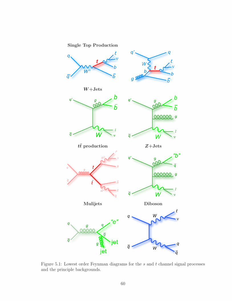
Single Top Production
W+Jets
tt production Z+Jets
Mulijets Diboson
Figure 5.1: Lowest order Feynman diagrams for the s and t channel signal processesand the principle backgrounds.
60

5.3 Modeling the QCD Multijet Background
As stated previously, the QCD multijet background is modeled using data. Two
samples are produced separatley, one for the electron channel and one for the muon
channel. These event samples are derived from a subset of the data which passes
almost all of the selection criteria. The samples are made orthogonal to the analysis
samples by inverting and removing some of the lepton identification cuts. For the
electron+jets channel the requirement for track matching is removed and the electron
likelihood cut is reversed to Le < 0.85. This allows the selection of fake electrons and
significantly increases the number of events for the QCD multijet sample. This also
distorts the shape of the lepton pT distribution. The method used to correct this
is discussed in Chapter 6. For muon+jets channel, the QCD sample is selected by
removing the muon and ∆R (µ, jet) requirements.
5.4 The Effects of the Top Mass Uncertainty
The top quark mass has a uncertainty of around 2 GeV [51]. This analysis is sensitive
to such a change in mass. To study this we have simulated single top and tt production
with three different top quark masses (170.0 GeV, 172.5 GeV and 175.0 GeV) [53].
The added benefit of this triples the statistics allowing a lower dependence on the top
quark mass. This new merged sample is only used to train Boosted Decision Trees
discussed in Chapter 7.
61

5.5 Determination of the W+Jets andMultijet Back-
ground Normilizations
The normilization of the single top and background samples other than W+Jets and
QCD multijets is done using the integrated luminosity and the cross sections listed in
Table 5.2. The W+Jets and QCD multijet are normalized to data using the equation:
N = λwjetsNwjets + λmultijetsNmultijets, (5.1)
where, N is the total number ofW+Jet and mulitjet events (N = NData−Nnon−wjets−MC),
λwjets and λmultijets are the nomalization scale factors which are anticorrelated. All
samples used here do not have any b tagging requirements. A simultaneous fit is
performed using three kinematic distributions which are sensitive to both λwets and
λmultijets. The distributions included in the fit are the lepton pT , /ET and the transverse
mass, MT (l, /ET ) [42]. In order to obtain values for both λs an iterative procedure is
used by first setting λwjets = 0 and solving for λmultijets using Eq. 5.1. A Kolmogorov-
Smirnov (KS) test is then used to measure the quality of the fit then repeated by
increasing λmultijets in steps of 0.001 to 4.0. The final normalization is chosen from the
fit result with the best combined KS fit for all three distributions. Table 5.3 shows
the final results used for RunIIa and RunIIb 2, 3 and 4 jet data samples and for the
electron and muon channels.
62

λwjets λmultijets
Run IIa Run IIb Run IIa Run IIbe µ e µ e µ e µ
2 jets 1.071 1.042 0.971 0.954 0.444 0.014 0.388 0.0343 jets 1.326 1.288 1.082 1.105 0.351 0.025 0.343 0.0454 jets 1.371 1.553 1.070 1.294 0.309 0.033 0.383 0.024
Table 5.3: Fitted W+Jets and QCD Multijet Scale Factors for each ofthe 24 fits.
63

5.6 Event Selection
The main point of the event selection cuts is to identify events that areW -like with one
isolated lepton, missing energy, and between two and four high pT jets. After a loose
preselection, the data is partitioned into samples with two, three and four jets. These
are collectively categorized as pertagged events, since no b tagging requirement has
been applied. The majority of the events areW+Jets with a small number of tt events
which dominate for higher jet multiplicities. Discussed below are the requirements
used for event preselection which are separated into three groups: general (applied to
all events), and electron (muon) channel which are additional cuts made specifically
for that channel.
5.6.1 General Preselection Requirements
Below are the general selection requirements used to pre-select data and simulated
events for the electron+jets and muon+jets channels.
For good quality data, runs that are identified as having detector or readout prob-
lems are rejected before any kinematic selections. Also, any runs having a negative
instantaneous luminosity is thrown out and the total integrated luminosity is cor-
rected for both effects.
Events are required to have at least one trigger firing in the OR list and have a
good primary vertex where |zPV| < 60 cm with at least three tracks connected to it.
This rejects events which are poorly defined trigger objects and that are at the edges
of the beamspot region. To be consistent with single top jet topology, it is required
that two to four jets have a pT > 15 GeV and exist in |ηdet| < 3.4. To remove some
of the backgrounds the leading jet must have a pT > 25 GeV. RunIIb has the highest
instantaneous luminosity, therefore additional cuts are made to remove fake jets and
64
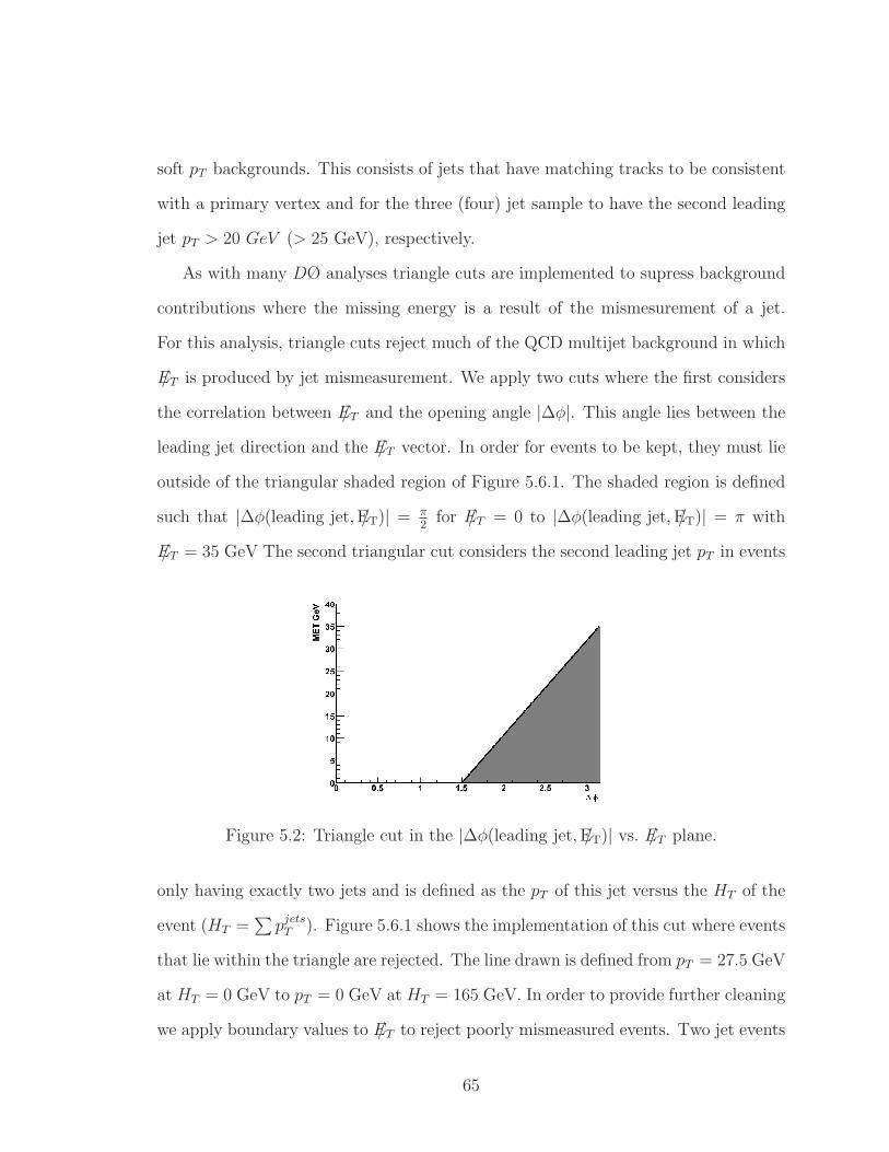
soft pT backgrounds. This consists of jets that have matching tracks to be consistent
with a primary vertex and for the three (four) jet sample to have the second leading
jet pT > 20 GeV (> 25 GeV), respectively.
As with many DØ analyses triangle cuts are implemented to supress background
contributions where the missing energy is a result of the mismesurement of a jet.
For this analysis, triangle cuts reject much of the QCD multijet background in which
/ET is produced by jet mismeasurement. We apply two cuts where the first considers
the correlation between /ET and the opening angle |∆φ|. This angle lies between the
leading jet direction and the /ET vector. In order for events to be kept, they must lie
outside of the triangular shaded region of Figure 5.6.1. The shaded region is defined
such that |∆φ(leading jet, /ET)| = π2for /ET = 0 to |∆φ(leading jet, /ET)| = π with
/ET = 35 GeV The second triangular cut considers the second leading jet pT in events
Figure 5.2: Triangle cut in the |∆φ(leading jet, /ET)| vs. /ET plane.
only having exactly two jets and is defined as the pT of this jet versus the HT of the
event (HT =∑
pjetsT ). Figure 5.6.1 shows the implementation of this cut where events
that lie within the triangle are rejected. The line drawn is defined from pT = 27.5 GeV
at HT = 0 GeV to pT = 0 GeV at HT = 165 GeV. In order to provide further cleaning
we apply boundary values to /ET to reject poorly mismeasured events. Two jet events
65

Figure 5.3: Triangle cut in the second leading jet pT vs. HT (alljets) plane.
are retained if their /ET lie between 20 GeV to 200 GeV and events with three to four
jets are kept if they lie between 25 Gev to 200 GeV.
Lastly, threshold cuts are required for eventHT (alljets) andHT (alljets, lepton, /ET ).
Also, these are implemented to reduce the background for soft QCD multijet events.
For HT (alljets) minimum thresholds of 50, 75 and 100 GeV are required for the two,
three and four jet events (RunIIa only). For RunIIb these are extended to 55, 80 and
110 GeV due to higher luminosity running conditions. For HT (alljets, lepton, /ET )
minimum thresholds of 120, 140 and 160 GeV are required for two, three and four jet
events for both RunIIa and RunIIb.
5.6.2 Electron+Jets Channel Preselection
For a candidate electron+jet event to be kept it is required to have one tight electron
with |ηdet| < 1.1 and pT > 15 that passes the tight electron ID requirements and is
consistent with primary vertex |∆z(e,PV)| < 1 cm. For events with ≥2 good jets the
pT is raised to 20 GeV. Events with an additional loose electron with pT > 15 GeV
and passes the loose electron definition are vetoed. Likewise, events with a tight
isolated muon with pT > 15 GeV and within |ηdet| < 2.0 are rejected as well. This
66
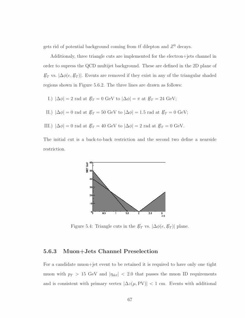
gets rid of potential background coming from tt dilepton and Z0 decays.
Additionaly, three triangle cuts are implemented for the electron+jets channel in
order to supress the QCD multijet background. These are defined in the 2D plane of
/ET vs. |∆φ(e, /ET )|. Events are removed if they exist in any of the triangular shaded
regions shown in Figure 5.6.2. The three lines are drawn as follows:
I.) |∆φ| = 2 rad at /ET = 0 GeV to |∆φ| = π at /ET = 24 GeV;
II.) |∆φ| = 0 rad at /ET = 50 GeV to |∆φ| = 1.5 rad at /ET = 0 GeV;
III.) |∆φ| = 0 rad at /ET = 40 GeV to |∆φ| = 2 rad at /ET = 0 GeV.
The initial cut is a back-to-back restriction and the second two define a nearside
restriction.
Figure 5.4: Triangle cuts in the /ET vs. |∆φ(e, /ET )| plane.
5.6.3 Muon+Jets Channel Preselection
For a candidate muon+jet event to be retained it is required to have only one tight
muon with pT > 15 GeV and |ηdet| < 2.0 that passes the muon ID requirements
and is consistent with primary vertex |∆z(µ,PV)| < 1 cm. Events with additional
67

loose muon with pT > 4 GeV and pass the loose muon requirements are vetoed.
Likwise, events with a loose electron that has pT > 15 GeV and within |ηdet| < 2.5
gets rejected. This gets rid of potential background coming from tt dilepton and Z0
decays.
The momentum of high pT muons can be severly miss measured, because of this
an additional track quality cut is required to reject events with this type of signature.
This cut is defined by imposing a restriction on the significance of the track curvature.
The track curvature is defined as:
|TrackCurvSig| = | q/pTσ(1/pT )
|, (5.2)
where, q and pT are the charge and transverse momentum of the charged track as-
sociated with the muon. RunIIa and RunIIb both have different values due to the
change in the amount of background considered in the tracker. There are two cuts
which are defined in the |TrackCurvSig| vs. |∆φ(µ, /ET )| plane. They are:
I.) |∆φ| from 0.875π to π rad when |TrackCurvSig| = 0, and |TrackCurvSig| from
0 to 4 (6) when |∆φ| = π rad for Run IIa (Run IIb) period;
II.) |∆φ| from 2 to π rad when |TrackCurvSig| = 0, and |TrackCurvSig| from 0 to
2 (3) when |∆φ| = π rad for Run IIa (Run IIb) period.
Additionaly, two triangle cuts are implemented to supress the QCD multijet back-
ground. Similar to the electron+jets channel, these are defined in the /ET vs. |∆φ(µ, /ET)|
plane. Events are removed if they exist in any of the triangular shaded regions shown
in Figure 5.6.3. The two bounding lines are drawn as follows:
I.) |∆φ| = 2.5 rad at /ET = 0 GeV to |∆φ| = π at /ET = 30 GeV;
II.) |∆φ| = 0 rad at /ET = 85 GeV to |∆φ| = 1.2 rad at /ET = 0 GeV;
68
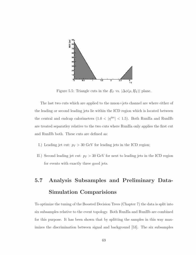
Figure 5.5: Triangle cuts in the /ET vs. |∆φ(µ, /ET)| plane.
The last two cuts which are applied to the muon+jets channel are where either of
the leading or second leading jets lie within the ICD region which is located between
the central and endcap calorimeters (1.0 < |ηdet| < 1.5). Both RunIIa and RunIIb
are treated separatley relative to the two cuts where RunIIa only applies the first cut
and RunIIb both. These cuts are defined as:
I.) Leading jet cut: pT > 30 GeV for leading jets in the ICD region;
II.) Second leading jet cut: pT > 30 GeV for next to leading jets in the ICD region
for events with exactly three good jets.
5.7 Analysis Subsamples and Preliminary Data-
Simulation Comparisions
To optimize the tuning of the Boosted Decision Trees (Chapter 7) the data is split into
six subsamples relative to the event topology. Both RunIIa and RunIIb are combined
for this purpose. It has been shown that by splitting the samples in this way max-
imizes the discrimination between signal and background [53]. The six subsamples
69
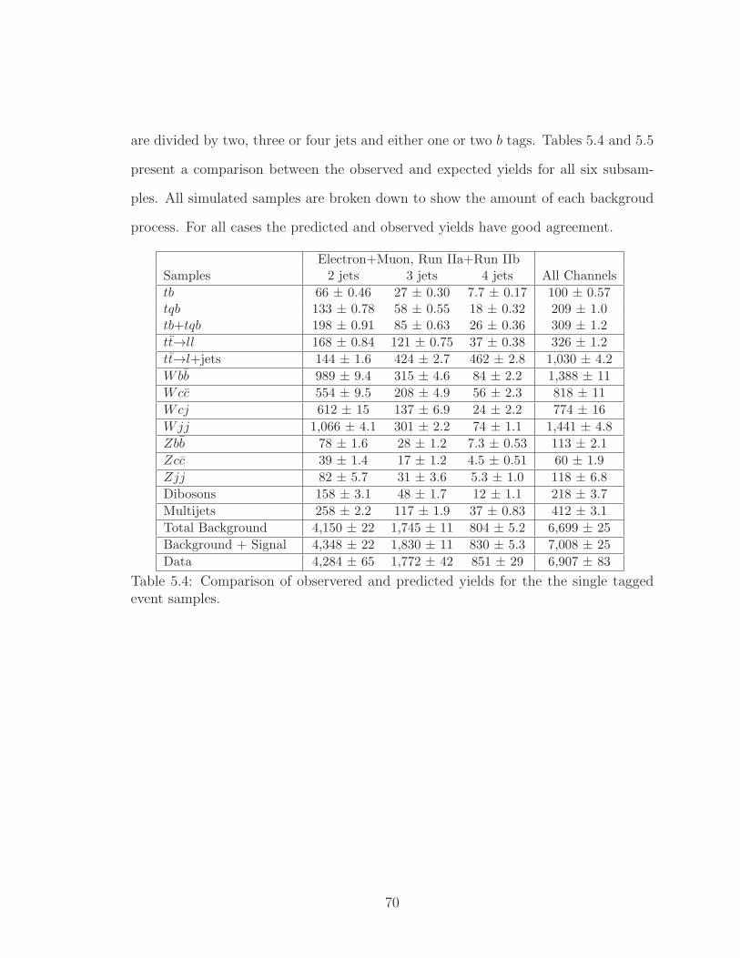
are divided by two, three or four jets and either one or two b tags. Tables 5.4 and 5.5
present a comparison between the observed and expected yields for all six subsam-
ples. All simulated samples are broken down to show the amount of each backgroud
process. For all cases the predicted and observed yields have good agreement.
Electron+Muon, Run IIa+Run IIbSamples 2 jets 3 jets 4 jets All Channels
tb 66 ± 0.46 27 ± 0.30 7.7 ± 0.17 100 ± 0.57tqb 133 ± 0.78 58 ± 0.55 18 ± 0.32 209 ± 1.0tb+tqb 198 ± 0.91 85 ± 0.63 26 ± 0.36 309 ± 1.2
tt→ll 168 ± 0.84 121 ± 0.75 37 ± 0.38 326 ± 1.2
tt→l+jets 144 ± 1.6 424 ± 2.7 462 ± 2.8 1,030 ± 4.2
Wbb 989 ± 9.4 315 ± 4.6 84 ± 2.2 1,388 ± 11
Wcc 554 ± 9.5 208 ± 4.9 56 ± 2.3 818 ± 11
Wcj 612 ± 15 137 ± 6.9 24 ± 2.2 774 ± 16
Wjj 1,066 ± 4.1 301 ± 2.2 74 ± 1.1 1,441 ± 4.8
Zbb 78 ± 1.6 28 ± 1.2 7.3 ± 0.53 113 ± 2.1
Zcc 39 ± 1.4 17 ± 1.2 4.5 ± 0.51 60 ± 1.9
Zjj 82 ± 5.7 31 ± 3.6 5.3 ± 1.0 118 ± 6.8
Dibosons 158 ± 3.1 48 ± 1.7 12 ± 1.1 218 ± 3.7
Multijets 258 ± 2.2 117 ± 1.9 37 ± 0.83 412 ± 3.1
Total Background 4,150 ± 22 1,745 ± 11 804 ± 5.2 6,699 ± 25
Background + Signal 4,348 ± 22 1,830 ± 11 830 ± 5.3 7,008 ± 25
Data 4,284 ± 65 1,772 ± 42 851 ± 29 6,907 ± 83
Table 5.4: Comparison of observered and predicted yields for the the single taggedevent samples.
70
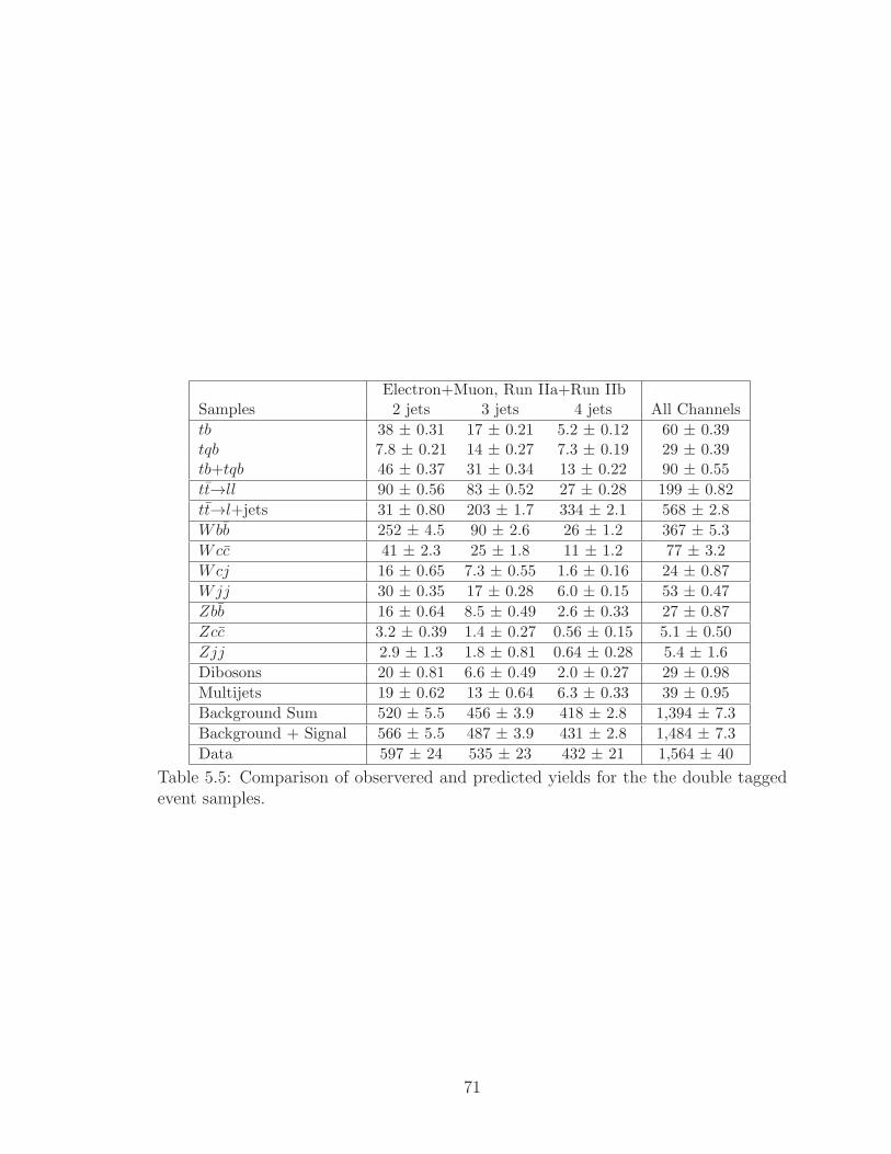
Electron+Muon, Run IIa+Run IIbSamples 2 jets 3 jets 4 jets All Channels
tb 38 ± 0.31 17 ± 0.21 5.2 ± 0.12 60 ± 0.39tqb 7.8 ± 0.21 14 ± 0.27 7.3 ± 0.19 29 ± 0.39tb+tqb 46 ± 0.37 31 ± 0.34 13 ± 0.22 90 ± 0.55
tt→ll 90 ± 0.56 83 ± 0.52 27 ± 0.28 199 ± 0.82
tt→l+jets 31 ± 0.80 203 ± 1.7 334 ± 2.1 568 ± 2.8
Wbb 252 ± 4.5 90 ± 2.6 26 ± 1.2 367 ± 5.3
Wcc 41 ± 2.3 25 ± 1.8 11 ± 1.2 77 ± 3.2
Wcj 16 ± 0.65 7.3 ± 0.55 1.6 ± 0.16 24 ± 0.87
Wjj 30 ± 0.35 17 ± 0.28 6.0 ± 0.15 53 ± 0.47
Zbb 16 ± 0.64 8.5 ± 0.49 2.6 ± 0.33 27 ± 0.87
Zcc 3.2 ± 0.39 1.4 ± 0.27 0.56 ± 0.15 5.1 ± 0.50
Zjj 2.9 ± 1.3 1.8 ± 0.81 0.64 ± 0.28 5.4 ± 1.6
Dibosons 20 ± 0.81 6.6 ± 0.49 2.0 ± 0.27 29 ± 0.98
Multijets 19 ± 0.62 13 ± 0.64 6.3 ± 0.33 39 ± 0.95
Background Sum 520 ± 5.5 456 ± 3.9 418 ± 2.8 1,394 ± 7.3
Background + Signal 566 ± 5.5 487 ± 3.9 431 ± 2.8 1,484 ± 7.3
Data 597 ± 24 535 ± 23 432 ± 21 1,564 ± 40
Table 5.5: Comparison of observered and predicted yields for the the double taggedevent samples.
71

Figure 5.7 shows the comparison of data with all the simulations for fifteen of the
variables used in the BDT analysis. Each comparison plot is a combination of all
six subsamples and show good agreement. At the split subsample level comparisons
similar to these also exhibit good agreement [42]. Figure 5.6 below presents the
colour scheme used throughout this analysis to label data, signal and background
events occuring in all plots.
Figure 5.6: Colour scheme plot key used to label Data, siganl and background eventsfor plots.
72
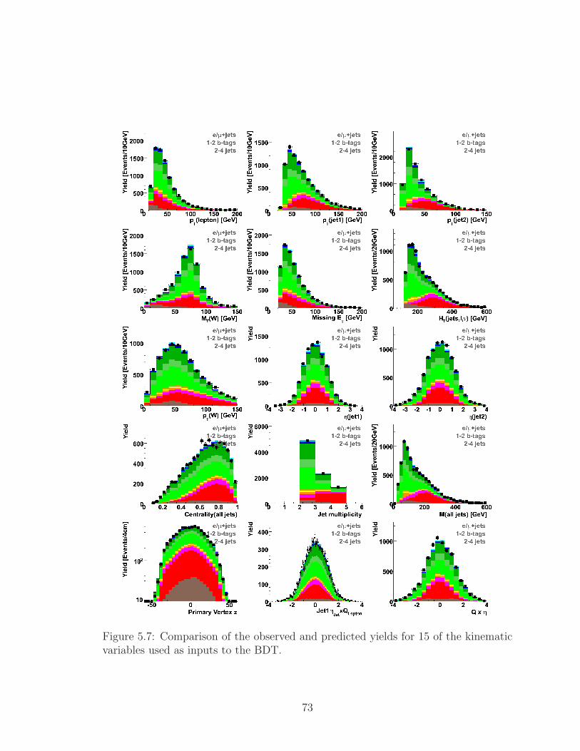
Figure 5.7: Comparison of the observed and predicted yields for 15 of the kinematicvariables used as inputs to the BDT.
73

Chapter 6
Monte Carlo Model Corrections
and Statistical Uncertainties
The DØ detector has been around for quite awhile where the effect of its aging is
present in the efficiencies of some of its components and resolution. The GEANT
model does take most of these effects into account, however it its not entirley correct
and additional corrections are needed to compensate for the residual differences. Cor-
rections to the underlying physics simulations are also needed to agree with current
values. These are discussed in the following sections.
6.1 Detector Response Corrections
Both RunIIa and RunIIb have different instantaneous luminosities. This is modeled
by adding together zero-bias events with corresponding simulated events. Because
zero-bias events are limited in size the MC instantaneous luminosity does not reflect
that of the instantaneous luminosity for data. Therefore, the MC instantaneous lumi-
nosity is reweighted to reflect the same value as data. Zero-bias events are recorded
74
data events which have no trigger requirements.
The position and size of the beam spot is also different for both run periods.
Specifically, when comparing these to simulated events we find that the primary
vertices z distributions are narrower than what is seen in data. Since this also affects
the acceptance calculations, a correction factor is given to simulated events so as to
be consistent with data. The correction factor is given as a function of instantaneous
luminosity and run period [54].
The electron identification efficiencies for monte carlo and data do not match,
with the former having higher efficiencies than that of data. Therefore, the monte
carlo events are reweighted using the equation
εe−ID =εDataPresel
εMCPresel
× εDataPostPresel
εMCPostPresel
(6.1)
where the terms in the correction are expressed in two parts, labeled preselection and
post preselection. The pre-selection ratio focuses on the electromagnetic fraction and
isolation efficiency contribution and is parametrized as a function of ηdet. The latter
ratio is parameterized in (ηdet, φ) and is determined by using a tag-and-probe analysis
of Z → ee events and takes account of the differences in the H-matrix term.
A similar correction is needed to obtain the muon identification efficiency values.
This is reweighted using the equation
εµ−ID =εDataReco
εMCReco
×εDataTrack|Reco
εMCTrack|Reco
×εDataIsolation|Track
εMCIsolation|Track
(6.2)
where each of the three correction terms relate to the uncertainties in the simulation of
the ID efficiency (Reco), the muon-central tracking matching efficiency (Track—Reco)
and the isolation efficiency (Isolation—Track), respectively. A tag and probe method
75

of Z → µµ events is used to determine each of these. The muon ID term is
parametrized as a function of (ηdet, φ), the track matching term in (z, ηCFT ) and
the isolation term in η [58, 59].
The simulation of the jet resolution also needs some adjustment to make it match
the data. For this analysis the DØ JSSR (Jet Smearing Shifting and Removal) is
used [60]. The re-weighting corrections are obtained from the comparison of simulated
and actual γ+jet events. These corrections are applied to each of the W+Jet, Z+Jet,
and diboson samples used in this analysis.
The last set of detector response corrections are used to match the simulated b
tagging efficiencies in monte carlo to those in data. The corrections are divided into
two parts for the b tagging process. Initially a jet must have enough information for
the b tagging algorithm to designate a jet as taggable, called the taggability efficiency.
Second is the efficiency for the algorithm to tag b jets, called the tagging efficiency.
Both these efficiencies are determined on a per jet basis from data and monte carlo
simulations. Ratios of the data and monte carlo effeciencies are then used to provide
the necessary correction factors. Since this procedure is quite involved, it is discussed
in detail below.
The taggability scale factor SFT can be defined as the number of taggable jets
divided by the total number of good jets. It is expressed in the form
SFT (pT , η, PVz) =T data(pT , η)
Tmc(pT , η), (6.3)
where T (pT , η) is the taggability efficiency as a function of the jet pT and η. SFT is
parametrized as a function of the jet pT , η, and the z position of the PVz. A scale
facotor can then be formed to preserve normalization for untaggable jets and is given
76

as:
SFT (pT , η, PVz) =1− T data(pT , η)
1− Tmc(pT , η). (6.4)
The scale factor per event can then be derived as:
NT∏
i=1
SFT (pT,i, ηdet,i, PVz,i)×NT∏
j=1
SFT (pT,j, ηdet,j , PVz,i), (6.5)
where NT and NT stand for the number of taggable and untaggable jets in each event.
To account for some of the correlations between the jets an additional correction,
SF (NT , NT ) is required, where:
SF (NT , NT ) =Edata(NT , NT )
EMC(NT , NT ). (6.6)
Here E represents the number of events in each sample. Thus the final taggability
scale factor is:
SF (NT , NT )×NT∏
i=1
SFT (pT,i, ηdet,i, PVz,i)×NT∏
j=1
SFT (pT,j, ηdet,j , PVz,i). (6.7)
This correction is applied to all of the simulated event samples.
The DØ b-ID provides the b tagging efficiencies for both data and monte carlo
events. These effecincies are a function of jet pT , η and the operating point of the
neutral network tagger, NNout. The following scale factors are then used to match
the monte carlo simulations to data:
SFtag(pT , η, NNout) =ǫdata(pT , η, NNout)
ǫmc(pT , η, NNout). (6.8)
77
Thus the per event scale factor is given by:
NT∏
i=1
SFtag(pT,i, ηi, NNout). (6.9)
NT is the number of taggable jets.
The regular b tagging algorithm is not used for the simulated W+light jets back-
ground due to the tagging algorithm accepting fake b tagged jets from this sample.
Using the regular b tagging algorithm would result in low statistical samples due to
the small fake probability. To get around this problem we use a random tagging tech-
nique [61]. This is implemented by selecting random untagged jets in the simulated
W+light jets samples and assigning them a 50% tag probability. All of the selected
jets which are taggable are then weighted using the appropriate scale factor.
6.2 Theoretical Uncertainties
This section provides a discussion for corrections made for various theoretical uncer-
tainties that have an affect on the background simulations. Specifically, the most
significant of these are the treatment of the W+heavy flavor background, the correc-
tions to the shape of the ZpT spectrum and the bias in the QCD multijet sample that
is used for the analysis in the electron channel.
The W+heavy flavor production cross sections are not accuratley known. This
must be considered because the W +bb background is sensitive to this analysis due to
the presence of real b quarks in events. In the previousDØ analysis [52], a heavy flavor
correction (λHF ) was measured and applied to the Wbb and Wcc samples to provide
better data-background agreement [52]. For this analysis studies were also performed,
resulting in a measured factor λHF=1 ± 12% [52]. Based on these measurements, a
78

correction was not needed, however its uncertainties are included.
alpgen [55] was used to simulate the Z+jets background. There is a difference in
shape of the ZpT spectrum between alpgen and current NLO predictions. Because
of this the simulated events are corrected so as to follow th NLO distribution.
The W+Jets and Z+Jets simulated backgrounds show good agreement with data,
however there are a few discrepancies in the the jet rapidity and angular correlations.
It is assumed that these discrepancies come about by using the leading log approxima-
tion in alpgen associated with the zero bias overlay being limited in the ICR region.
These discrepancies are corrected by applying a reweighting factor Ri to simulated
events before the b tag requirements. Each distribution is reweighted in the ith bin
and is defined by
Ri =Ni
NV+jets,i
, (6.10)
where, Ni is the number of observed events minus the predicted yields from all pro-
cesses other than W and Z+Jets (Ni = NData,i−NQCD+non−vjets,i). Nvjets,i is the sum
of the W and Z+Jets predicted event yields in bin i. These ratios are then plotted for
each of the angular distributions to be corrected and fitted to determine a reweighting
function. Five distributions are considered: η(jet1), η(jet2), ∆R(jet1, jet2), η(jet3)
and η(jet4). The reweighting is done sequentially, starting with η(jet1) and ending
with η(jet4), where η(jet3) and η(jet4) are used in the three jet and four jet sam-
ples, repectively. For a more detailed discussion of the reweighting process please see
reference [42].
The QCD multijet sample used for the electron channel analysis was derived from
data by applying all standard electron requirements except for the track matching
requirement and the electron likelihood cut, which was inverted (Le < 0.85). This
introduces a kinematic bias coming from fake electrons which needs to be corrected.
79
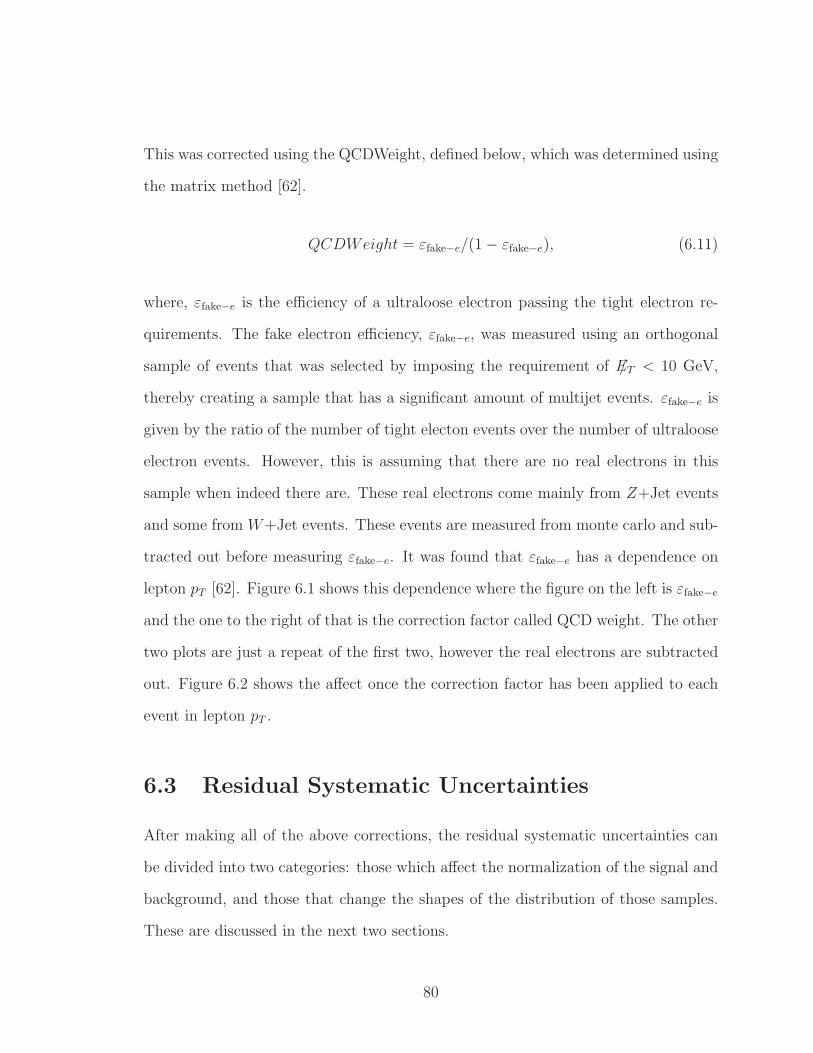
This was corrected using the QCDWeight, defined below, which was determined using
the matrix method [62].
QCDWeight = εfake−e/(1− εfake−e), (6.11)
where, εfake−e is the efficiency of a ultraloose electron passing the tight electron re-
quirements. The fake electron efficiency, εfake−e, was measured using an orthogonal
sample of events that was selected by imposing the requirement of /ET < 10 GeV,
thereby creating a sample that has a significant amount of multijet events. εfake−e is
given by the ratio of the number of tight electon events over the number of ultraloose
electron events. However, this is assuming that there are no real electrons in this
sample when indeed there are. These real electrons come mainly from Z+Jet events
and some from W+Jet events. These events are measured from monte carlo and sub-
tracted out before measuring εfake−e. It was found that εfake−e has a dependence on
lepton pT [62]. Figure 6.1 shows this dependence where the figure on the left is εfake−e
and the one to the right of that is the correction factor called QCD weight. The other
two plots are just a repeat of the first two, however the real electrons are subtracted
out. Figure 6.2 shows the affect once the correction factor has been applied to each
event in lepton pT .
6.3 Residual Systematic Uncertainties
After making all of the above corrections, the residual systematic uncertainties can
be divided into two categories: those which affect the normalization of the signal and
background, and those that change the shapes of the distribution of those samples.
These are discussed in the next two sections.
80
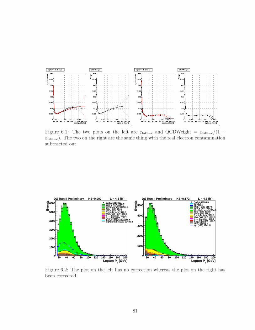
Figure 6.1: The two plots on the left are εfake−e and QCDWeight = εfake−e/(1 −εfake−e). The two on the right are the same thing with the real electron contaminationsubtracted out.
[GeV]T
Lepton P20 40 60 80 100 120 140 160 180 200
Eve
nts
0
1000
2000
3000
4000
5000
6000
20 40 60 80 100 120 140 160 180 2000
1000
2000
3000
4000
5000
6000 DATA 50170.0Wbb + jets 1278.7Wcc + jets 2887.6W + light jets 40799.9Zbb + jets 114.7Zcc + jets 110.2Z + light jets 1919.3WW / WZ / ZZ 1012.0
dilepton 167.7→ tt lep + jets 173.0→ ttQCD 1745.7
signal: tb (x100) 6588.5signal: tqb (x100) 12480.8
DØ Run II Preliminary L = 4.3 fb -1KS=0.000
[GeV]T
Lepton P20 40 60 80 100 120 140 160 180 200
Eve
nts
0
1000
2000
3000
4000
5000
20 40 60 80 100 120 140 160 180 2000
1000
2000
3000
4000
5000DATA 42984.0tb 64.4tqb 124.2Wbb + jets 1187.6Wcc + jets 2660.7W + light jets 32634.0Zbb + jets 132.8Zcc + jets 289.3Z + light jets 2999.3WW / WZ / ZZ 1082.3
dilepton 158.5→ tt lep + jets 159.4→ tt
QCD 1487.6tb (x10) 643.6tqb (x10) 1241.8
DØ Run II Preliminary L = 4.3 fb -1KS=0.172
Figure 6.2: The plot on the left has no correction whereas the plot on the right hasbeen corrected.
81
6.3.1 Normalization Effects
There are two luminosity uncertainties that affect this analysis. The calculation of the
integrated luminosity has an uncertainty of ±6.1%. This uncertainty was calculated
using RunIIa data where the main contribution is due to the ±5.4% uncertainty in
the knowledge of the inelastic pp cross section [63, 64]. The ±6.1% uncertainty is
then obtained by adding in quadrature the ±5.4% uncertainty with the uncertainties
which come from the modeling of the radiation damage to the luminosity monitor.
Additionally there is an uncertainty of ±1%, which originates in the reweighting
process used to model the differences in the instantaneous luminosity within the Run
IIa and IIb simulations.
The theoretical cross sections pertaining to this analysis also have an uncertainty.
For signal and tt the uncertainties are calculated in Refs. [65, 66]. These are cal-
culated by summing in quadrature the uncertainties due to the factorization scales,
kinematics, PDF and the knowledge of the top quark mass. For a nominal top quark
mass of 172.5 GeV the uncertainties are ±3.8% for the s channel, ±5.3% for the t
channel, ±4.8% for the the combined s and t channels and +6.4−9.0% for tt pair produc-
tion. The ±7.0% uncertainties in the diboson (WW , WZ, ZZ) cross sections are
taken from the values used by the DØ Higgs group [42]. The Z+Jets cross section
uncertainty is set to ±3.3% using with the results from reference [42].
The signal acceptance has an uncertainty of ±2.0% coming from the PDFs. This
was calculated by reweighting monte carlo events using 40 different CTEQ PDFs
and then calculating the acceptance with each PDF. The uncertainty was conserva-
tively estimated by taking the maximum change in the acceptance between the 40
PDF results. The PDF uncertainties for tt, diboson and Z+Jets are included in the
theoretical cross section uncertainties for each.
82

The uncertainty on branching fractions for aW boson decaying to any given lepton
is taken from the PDG results [1]. This gives an average uncertainty of ±1.5% which
is added into the uncertainties for monte carlo normalization.
The trigger efficiency for this analysis is approximatley∼100% with an uncertainty
of ±5.0%. The uncertainty was obtained by looking at the efficiencies of several
variables wich are sensitive to the triggers. Nearly all efficiencies lie between 95% and
105% and ±5.0% is taken as the representative uncertainty. The trigger efficiency
plots used in this estimate can be seen in Ref. [42].
There are two different uncertainties attributed to the primary vertex, one of
modeling and the other, selection. The primary vertex distribution in monte carlo is
reweighted to match that of data [54]. This reweighting has a ±0.05% uncertainty.
The selection efficiency for the primary vertex differs between monte carlo and data.
The uncertainty in this difference gives an additional uncertainty of ±1.4% [54].
The uncertainties for the electron and muon scale factors have been determined by
the DØ electron and muon ID groups using tag and probe methods. For electrons the
scale factor uncertainty is ± 4.8% [67], and for muons the corresponding uncertainty
is ± 2.1% [42, 68].
The effects of modeling color reconnection has an uncertainty. This is assessed by
comparing the results from the tune A Pro and tune AC Pro versions of the pythia
generator. Tune A Pro does not account for reconnection effects, whereas Tune AC
Pro does try to model them. The difference in the two values for a top mass analysis
is ± 1.0%, which is taken as the estimated uncertainty [69].
The uncertainties due to jet fragmentation and higher order affects were esti-
mated by comparing the acceptances for tt events using different monte carlo gen-
erators. For this study, events from alpgen+pythia were compared to those from
alpgen+herwig. This results in uncertainties of ±0.7%, ±3.7% and ±4.7% for the
83

two, three and four jet bins for the signal, Z+Jets and diboson samples. By including
the effects of higher order QCD contributions an estimation of those effects can be ob-
tained by comparing events from alpgen+herwig and MC@NLO+herwig. This
gives additional uncertainties of ±1.6%, ±1.7% and ±7.0% for the two, three and
four jet bins, respectively. These are applied to the tt samples used in this analysis.
tt samples were also used to estimate the uncertainties in the modeling of the initial
and final state radiation. This is done by generating a number of tt acceptances while
changing the ISR/FSR settings in pythia. These are then compared to the values
generated with the nomianl settings to measure the uncertainty. Taking into account
jet multiplicity the uncertainty ranges from ±0.8% to ±10.9% for the two, three and
four jet bins, respectively.
By taking into account what is known about b jet fragmentation, uncertainties
can be estimated using tt simulations. This is done by changing the tune settings of
the Bowler fragmentation function used by pythia [70]. By comparing the results of
the SLD and LEP tunes, the b fragmentation uncertainty was estimated to be ±2.0%.
This uncertainty is applied to the signal, tt and Zbb samples.
The uncertainty for the relative b/light jet response can be measured by first
taking the double ratio of the b and light jets pTs (measured from response) from a
simulated tt sample, given by:
(pDataT
pMCT
)b−jet
(pDataT
pMCT
)light−jet
. (6.12)
This results in a difference of ±1.8% [71]. The b jets response is then shifted down by
1.8% to to correct for this. The corresponding uncertainties are taken from the DØ
tt cross section analysis [72]. This gives uncertainties of ±0.4% (2 or 3 jet events) and
±0.3% (4 jet events). For single top, the corresponding uncertainties were measured
to be ±0.5%, ±0.8% and ±0.9% for two, three and four jet events, respectively.
84

Lastly, the Zbb sample has uncertainties of ±1.0%, ±0.6% and ±0.8% for two, three
and four jet topologies.
The uncertainty on the taggability efficiencies are measured by fluctuating the
scale factor up and down by one sigma for each monte carlo sample. The whole
analysis is repeated for both up and down samples and uncertainties range from
±3.1% to ±21.5% [42], where the range corresponds to one tag 2, 3 and 4 jet samples
and two tag 2, 3 and 4 jet samples.
The W+Jets heavy scale factor (λHF ) is used as an additional correction to the
Wbb and Wcc monte carlo samples. For this analysis it is measured with an uncer-
tainty of ±12.0% [42]. For a detailed discussion please see Ref. [42]. The uncertainty
on the Z+Jets heavy scale factor is measured in a similar fashion to that of W+Jets
and is also found to be ±12.0%.
The uncertainty coming from both W+Jet and QCD multijet normalizations is
calculated by comparing the final scale factors to ones that vary the most. This is
done separatley for each variable in both event samples. The resulting uncertainty
in the W+jets normalization is ±1.8% and for the QCD multijet normalization is
between 30 and 40%.
Sample statistics uncertainty is due to the finite size of both the data and monte
carlo samples and is given by 1√N. This uncertainty is considered in the final discrim-
inant output for each background sample.
6.3.2 Shape-changing Effects
The vertex confirmation (VC), jet energy scale (JES), jet energy resolution (JER), b
tagging (BTag) and angular corrections (AC) result in simulation changes which not
only change the sample yield (normaliztion), but also change the shape of some of
85

the kinematic distributions. The uncertainties due to these are estimated by running
the whole analysis for each correction, producing two samples for each, one that
fluctuates the corrections up one sigma and another down one sigma. The uncertainty
is taken as the difference in fractional yield between each of these and the nominal
simulated sample. The jet reconstruction and identification (JetID) shape uncertainty
is estimated by first not applying the jet ID correction factor. This produces a
systematic sample which is compared to the nominal sample in an MVA output. The
difference between the two is then cut in half where JetIDup is the nominal plus one
half and JetIDdown is the nominal minus one half.
The b tagging uncertainty is estimated from the uncertainty in the taggability
and tagging scale factors added in quadrature. The origin of these uncertainties is
the limited statistics of the event samples used to calculate the scale factors. The
uncertainty for single tagged events ranges from ±4.3% to ±14.0% for 2, 3 and 4 jets,
and for double tagged events ±5.8% to ±11.2% for 2, 3 and 4 jets.
The V+Jets angular correction procedure preserves the normalization of the W
and Z+Jets pretag samples. By b tagging these samples a normalization uncertainty
is introduced through the b tagging scale factors, giving a normalization uncertainty
of ±0.3%.
Uncertainties for jet reconstruction and identification originate from the depen-
dence on the primary vertex, luminosity and the calculated jet efficiencies. These
combine to give a normalization uncertainty of between ±0.04% and ±3.7%, where
the range corresponds to the 2, 3 and 4 jet samples. The uncertainty coming from the
JER corrections comes mainly from fits used to measure the resolution and depen-
dence on the luminosity [73]. The normalization uncertainty here ranges from ±0.2%
to ±11.6%, where the range corresponds to the 2, 3 and 4 jet samples.
The JES corrections introduce an uncertainty of between ±0.3% and ±14.6%,
86

where the uncertainty comes from the uncertainties in all of its correction factors [74]
The final uncertainty considered here is that indroduced by the vertex confirma-
tion. The precision of this correction is limited by the size of the samples used in its
calculation. For instance, very forward jets are complicated because there is almost
no tracker and only a few jets can be confirmed, which makes it harder to derive a cor-
rection, and consequently an increased uncertainty. These uncertainties lie between
±0.1% and ±9.6% which corresponds to the position of the jet in the detector.
6.3.3 Summary of Residual Uncertainties
Table 6.1 presents an overall summary of the residual uncertainties. Detailed lists of
the source and its uncertainties as a function of tag and jet multiplicity can be seen
in the tables of Appendix B. The second part of Appendix B presents several plots
showing the shape changing effects of these uncertainties that are present in the BDT
discriminants used for the s, t and the combined s+ t channel analyses.
87

Source Uncertainty %Normalization UncertaintiesIntegrated luminosity 6.1tt cross section 9.0Z+jets cross section 3.3WW , WZ, ZZ, cross sections 7.0Branching fractions 1.5Parton distribution functions 2.0(signal acceptances only)Triggers 5.0Instantaneous luminosity reweighting 1.0Primary vertex selection 1.4Color reconnection 1.0b/light jet response (0.3-1.0)Electron identification (2.8-3.8)Muon identification 2.1Jet fragmentation and higher order effects (0.7-7.0)ISR and FSR corrections (0.8-10.9)b-jet fragmentation 2.0Taggability (3.1-21.5)W+jets heavy-flavor correction 12.0Z+jets heavy-flavor correction 12.0W+jets normalization 1.8QCD multijet normalization (30-40)MC and multijets statistics (0.2-16)
Normalization and Shape UncertaintiesJet reconstruction and identification (0.04-3.7)JER corrections (0.2-11.6)JES corrections (0.3-14.6)Vertex confirmation (0.1-9.6)b tagging (single tag) (4.3-14.0)b tagging (double tag) (5.8-11.2)Angular correction 0.3
Table 6.1: Residual systematic uncertainties after improvements to detector and pro-cess simulations. Where ranges are given, these correspond to 2, 3 and 4 jet events.
88

Chapter 7
Boosted Decision Trees
7.1 Introduction
Once the selection and b tagging requirements have been applied (Chapter 5) the
signal to background ratio is around 1:20. In a traditional analysis further cuts are
applied to obtain a suitable S:B ratio (cut based analysis). However in this case
this proves ineffective as the excess of signal is smaller than the predicted background
uncertainty. Also, signal is lost when additional cuts are applied making the cut based
approach impractical for a singletop cross section measurement. In this analysis a
multivariate analysis (MVA) technique called Boosted Decision Trees (BDT) is used
for the anlyses optimization. BDTs take as input selected variables for each event
and provide an output dicriminant between 0 and 1, where events closer to 0 tend to
be background whereas events closer to 1 tend to be signal.
Historically decision trees first came to light within the statistics community in
1963 [75] and later became more popular in the 1980s as data mining and machine
learning algorithms [76]. It was not until the 1990s when more sophisticated decision
tree algorithms were developed such as boosted decision trees [77]. Boosted deci-
89
sion trees were first used in the high energy physics community by the MiniBooNE
experiment [78, 79].
Figure 7.1 shows an example of how a decision tree is created. It starts off with
an initial node which applies a cut criteria where events pass if their HT < 242 GeV
and fail if HT ≥ 242 GeV. The cut is chosen such that it maximizes the separation
between signal and background events in the initial data sample. This cut creates two
daughter nodes where new criteria can be applied to separate signal from background
for these nodes. The process is continued until ceartin criteria are not met which turns
the node into a terminal leaf. These criteria will be discussed later on in this chapter.
The leaf then represents the discriminant output value D(~xi) where ~xi corresponds
to the variables used to obtain that value. This is also referred to as the purity which
is defined as:
p =Σisi
Σisi + bi=
sleafsleaf + bleaf
, (7.1)
where si and bi are the weighted sums of signal and background events for the leaf.
This whole process is continued until all nodes become terminal leafs, thereby creating
a tree. This process is also called decision tree training.
The training of a single tree does not provide enough separation power between
signal and background for this analysis, however this can be enhanced by using the
technique called boosting. Boosting basically creates a forest of trees by reweighting
the misclassified events wihin the tree. All of the trees created by boosting are then
averaged for the final output. This recovers misclassified events and gives a smoother
approximation to the final discriminant output. It is discussed in more detail in
Section 7.3.2.
Some of the advantages for using decision trees in an anlysis are that events which
would be rejected in a cut based analysis are still retained. BDTs make it easy to
90
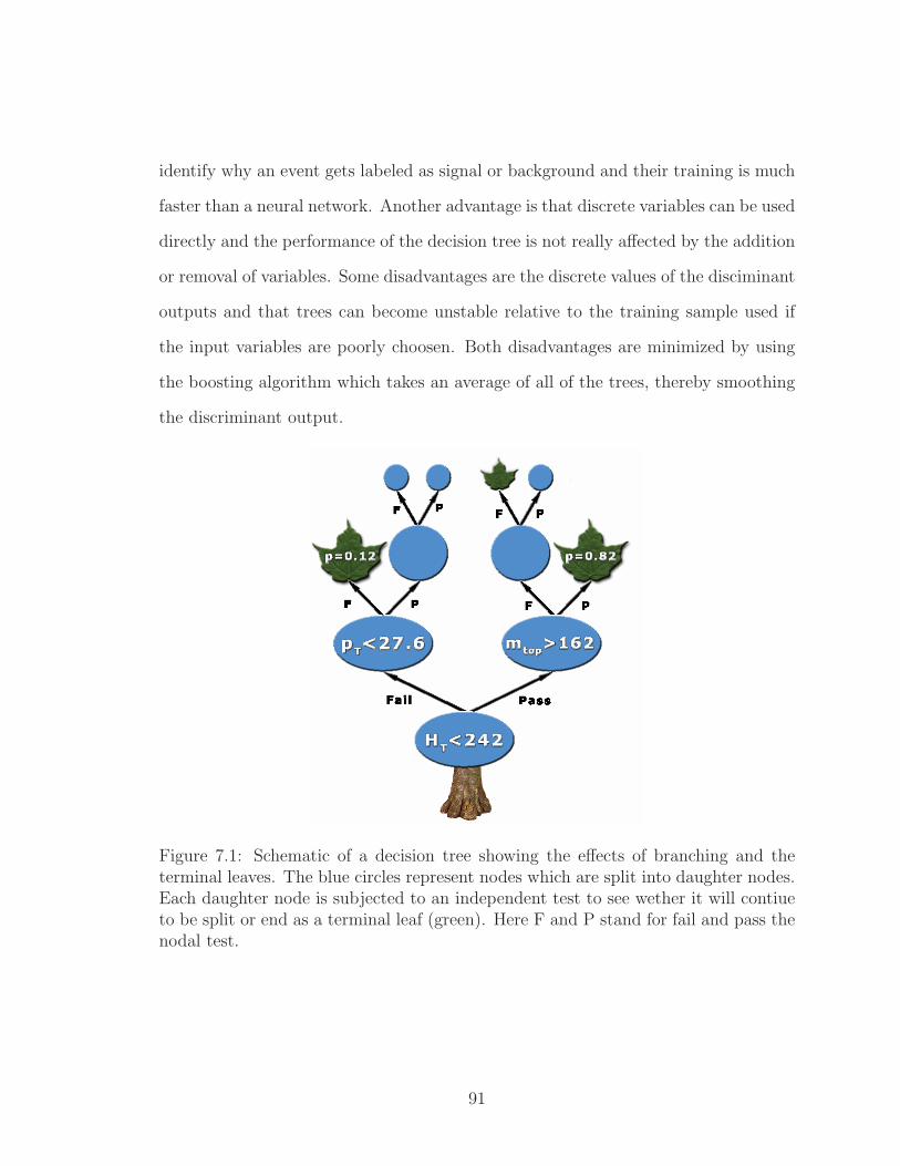
identify why an event gets labeled as signal or background and their training is much
faster than a neural network. Another advantage is that discrete variables can be used
directly and the performance of the decision tree is not really affected by the addition
or removal of variables. Some disadvantages are the discrete values of the disciminant
outputs and that trees can become unstable relative to the training sample used if
the input variables are poorly choosen. Both disadvantages are minimized by using
the boosting algorithm which takes an average of all of the trees, thereby smoothing
the discriminant output.
Figure 7.1: Schematic of a decision tree showing the effects of branching and theterminal leaves. The blue circles represent nodes which are split into daughter nodes.Each daughter node is subjected to an independent test to see wether it will contiueto be split or end as a terminal leaf (green). Here F and P stand for fail and pass thenodal test.
91

7.2 Sample Preparation
Three independent monte carlo subsamples are used for this analysis. These are
created by dividing the MC signal and background samples into three separate data
sets. The first of these is called the “training sample” and is used to train the BDTs.
The second is the “testing sample” which is used to train the MVAs used to combine
differennt BDTs. The third is called the “yield sample” and is used to calculate all
final cross section measurements. The data sample is unchanged and the simulated
samples are the only ones used in this way. The monte carlo datasets are split such
that the first event goes to the testing sample, the second the training sample and
the third and fourth are taken by the yield sample. This process is iterated until all
of the available events have been assigned. In total one fourth of all the MC samples
go to the training, one fourth to the testing and one half to the yield samples. Each
sample is then normalized back to the nominal luminosities set by multiplying the
training and testing samples by four and the yield sample by two.
7.3 Training
By using the training sample we can define an algorithm which describes how a de-
cision tree is built. Initially signal and background samples are normalized relative
to one another taking account of the normalization scales and correction factors dis-
cussed in Chapter 6. A node is then produced with both signal and background
events. A list of variables is then read into the BDT code where the variables have
been chosen to provide the best discrimination between signal and background. If no
splitting values are found that provide sufficient signal:background separation then
the node is defined to be a terminal leaf. If the data at a node can be split, then one
92

daughter node contains the events that pass the cut and one that fail the cut. If the
number of events in either daughter node falls below the minimum required, then the
node becomes a terminal leaf. This process is repeated many times until all of the
remaining daughter nodes have become terminal leafs. Each leaf is then assigned a
purity value using equation 7.1. This is shown schematically in Figure 7.1.
7.3.1 Splitting a Node
The splitting of a node into two daughters is by far the most significant and powerful
part in the training of a decision tree. This is done by first measuring the sample
impurity at the node. For this analysis the Gini Index [80] was used for this where:
G =sb
s+ b. (7.2)
Similar to the purity measure, s and b are the weighted sum of both signal and
background events for each node. Other impurity indexes are available, however it
has been shown that the Gini Index provides the best performance for this type of
analysis [80]. The best separation corresponds to the largest change of impurity ∆G
which is defined by:
∆G = G−GP −GF =sb
s+ b− sP bP
sP + bP− sF bF
sF + bF, (7.3)
where the subscripts P and F represent pass and fail for the daughter nodes created
by the split. A cut value is chosen such that it maximizes ∆G, thereby providing the
best separation between signal and background. This is done initially by reading in
the list of variables and sorting the events in the node relative to the variable being
used. ∆G is then calculated by going through each event in order and the highest
93

∆G is recorded. The algorithm moves to the next variable in the input list and the
process is repeated until the variable list is exhausted. The best ∆G is used to define
the nodal split.
7.3.2 Boosting
Boosting is used in this analysis to overcome some of the limitations previously stated.
It has also been shown to increase the overall performance by 20% [80]. The basic idea
behind boosting is to create an initial decision tree and then identify the misclassified
events within the tree. Misclassified events are then reweighted and a new decision
tree is created. This process is repeated until 30 trees are produced. Thirty repre-
sents the number of boosting cycles and was chosen because it gives the overall best
performance. The trees are then averaged to provide the final discriminant output.
Several different types of boosting algorithms are available in the literature, however
for this analysis the AdaBoost algorithm was chosen [77].
The AdaBoost algorithm works by first creating an initial decision tree. The
discriminant output of that tree is then used to find misclassified events by using the
relation |D(~xi)−zi| > 0.5 where zi is 1 (0) for signal (background). A misclassification
error (ǫn) is then calculated for the discriminant output as a weighted fraction of the
misclassified events. Using this error a tree weight is defined by:
αn = β × ln1− ǫnǫn
, (7.4)
where β is known as the boosting parameter. Each of the misclassified events are then
reweighted by eαn (which is always greater than one). A new decision tree is then
trained focusing on the misclassified events. This process is repeated for 30 cycles,
producing thirty decision trees. The decision trees are then averaged to obtain the
94
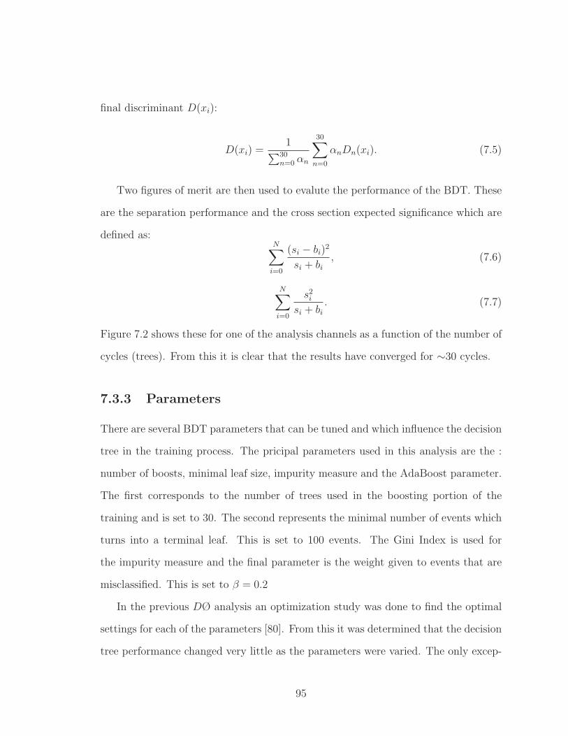
final discriminant D(xi):
D(xi) =1
∑30n=0 αn
30∑
n=0
αnDn(xi). (7.5)
Two figures of merit are then used to evalute the performance of the BDT. These
are the separation performance and the cross section expected significance which are
defined as:N∑
i=0
(si − bi)2
si + bi, (7.6)
N∑
i=0
s2isi + bi
. (7.7)
Figure 7.2 shows these for one of the analysis channels as a function of the number of
cycles (trees). From this it is clear that the results have converged for ∼30 cycles.
7.3.3 Parameters
There are several BDT parameters that can be tuned and which influence the decision
tree in the training process. The pricipal parameters used in this analysis are the :
number of boosts, minimal leaf size, impurity measure and the AdaBoost parameter.
The first corresponds to the number of trees used in the boosting portion of the
training and is set to 30. The second represents the minimal number of events which
turns into a terminal leaf. This is set to 100 events. The Gini Index is used for
the impurity measure and the final parameter is the weight given to events that are
misclassified. This is set to β = 0.2
In the previous DØ analysis an optimization study was done to find the optimal
settings for each of the parameters [80]. From this it was determined that the decision
tree performance changed very little as the parameters were varied. The only excep-
95

Number of trees included0 5 10 15 20 25 30
Sep
arat
ion
0.21
0.22
0.23
0.24
0.25
0.26
0.27
0.28
0.29
Separation vs number of trees included
Number of trees included0 5 10 15 20 25 30
Cro
ss S
ectio
n S
igni
fican
ce
1.55
1.6
1.65
1.7
1.75
1.8
1.85
1.9
1.95
Cross Section Significance vs number of trees included
Figure 7.2: Example plots showing separation power and cross section significanceversus the number of boosts.
96
tion was the effect of changing the number of boosting cycles. Because of this a new
study was performed for this analysis and it was found that 30 boosting cycles showed
optimal performance. The other parameters values were set to the same values as
were used in the previous DØ analysis [80].
7.3.4 Implementation
Decision trees are created and evaluated using the code package classifier located in
the DØ CVS code repository. Previous DØ Single Top Groups have also used this
code resulting in evidence and observation publications [80, 81]. The differences with
the code used for this comes mainly from the improvements and options which were
added to cope with large output files and the production of extensive plot lists for
each channel.
7.3.5 Selection of Input Variables
Selecting the input variables is a very important step in the definition of a BDT. The
variables must be chosen so as to effectively separate signal and background. If the
list of variables is too small, then the outcome is reflected in poor separation power.
On the other hand the addition of extra variables may have a negligible effect, unless
they have siginificant discrimination power. The addition of variables also makes
the training process more complex and slows down the construction of decision trees.
Because of this it is important to optimize both the number and the choice of variables
in order to minimize the complexity of the decision tree process. Fifty input variables
were chosen and used in the creation of decision trees for this analysis. To reduce the
added complexity, these same fifty variables are used for each of the six 1 tag×2,3
and 4 jet and 2 tag×2,3 and 4 jet channels.
97

The variable selection is divided into two steps. The first uses the ROOT imple-
mentation of the Kolmogorov-Smirnov (KS). This compares the data and simulated
distributions for any variable chosen by applying a quality test to determine if they
come from the same underlying distribution. The test gives a value between 0 and 1
where values closer to 0 suggest that the MC and data do not come from the same
underlying function and 1 suggests that they do and are typically well modeled. The
second step uses the BDT ranking method where each variable is assigned a ∆G
value. This is used to select the variables which provide the best separation between
signal and background. The combination of both these steps result in the list of fifty
input variables which were chosen for the analysis.
The first step is implemented by considering the KS value for all variables in each
of the six analysis channels. The KS values for each variable are added and then
divided by six to give the average for each variable. Only variables having an average
KS value ≥ 0.30 are kept for further analysis and individulal KS values < 0.01 are
rejected. This step provides a list of 136 variables which passes to the final BDT
ranking.
For the second step the list of 136 variables was used as inputs to train six BDTs,
one for each channel. Each BDT yields 30 trees, resulting in a ∆G sum over 180
calculations, per variable. The ∆Gs were then added and averaged and the fifty
variables with the highest ∆G were retained for the analysis. The data/MC distri-
butions for the fifty selected variables are shown in Figs 7.3-7.6 and they are listed
in Tables 7.1- 7.7 where they have been grouped into topological categories. A brief
discussion on the nomenclature of the variables is given below.
Jets are indexed by the order of their pT . For instance, jet1 has the highest pT ,
jet2 the second highest. The label “best” jet means the invariant mass M (W ,jet) is
the jet that gives a top quark mass closest to 172.5 GeV. Each event has one best
98

jet where the others are labeled “not best”. For once tagged samples, labels such as
“leading tagged jet” and “most b like jet” correspond to jets passing the b tagging
requirements, also the most b like jet is a jet with the highest BNN output. For twice
tagged samples, labels such as “leading tagged jet” and “second tagged jet” refer
to the order of their pT as well as passing the b tagging requirements. Labels such
as “leading light quark jet” and “second leading light quark jet” refer to jets which
are not b tagged and are also ordered by pT . Both the top quark and W boson are
reconstructed for many of the variables. The top quark is reconstructed using the
combined four vectors of the lepton, jet and nuetrino. The W boson is reconstructed
by using the lepton four momentum and the reconstructed neutrino pz. The neutrino
pz is unknown in the detector, however it can be estimated using the lepton four
momentum and the mass of the W . The pz solution found is quadratic yielding two
solutions. The first solution is labeled S1 and is chosen as the lower of the two values.
The second solution is labeled S2. Typically S1 is used.
99

Kinematic VariablesLeading Light Quark Jet E: Leading light quark jet energyηdet (jet1): ηdet fo the most b like jetη width (jetmost b like): Width of the most b-like jet in ηη width (jetnot best 1): Not the best leading jet width in ηpT (lepton): pT of the leptonpT (jetbest): pT of the best jetB tag NNBest Jet: NN output of the best jetLepton φdet direction: φdet of the leptonNeutrino pz: first solution for pz of the neutrino (S1)Not Best 1 φ width: Not the best leading jet width in φNot Best 2 φ width: Not the best 2nd leading jet width in φ
Table 7.1: List of individual object kinematics.
Event VariablesRun Period: RunIIa vs. RunIIb
Centrality (all jets):∑
HT∑E
Missing ET : pT of the /ET
Missing ET phi direction: φ direction of the /ET
Primary vertex z: Primary vertex position of z
Table 7.2: List of event variables.
Charge of the lepton times η
Q× η: of the leading light jetQ(lepton)× η(lepton): of the leptonQ(lepton)× η(best1): of the most b like jetJet1 ηjet ×Qlepton: of the leading jetNot Best 1 ηjet ×Qlepton: of not the best leading jet
Table 7.3: List of variables using the sign of lepton charge.
100
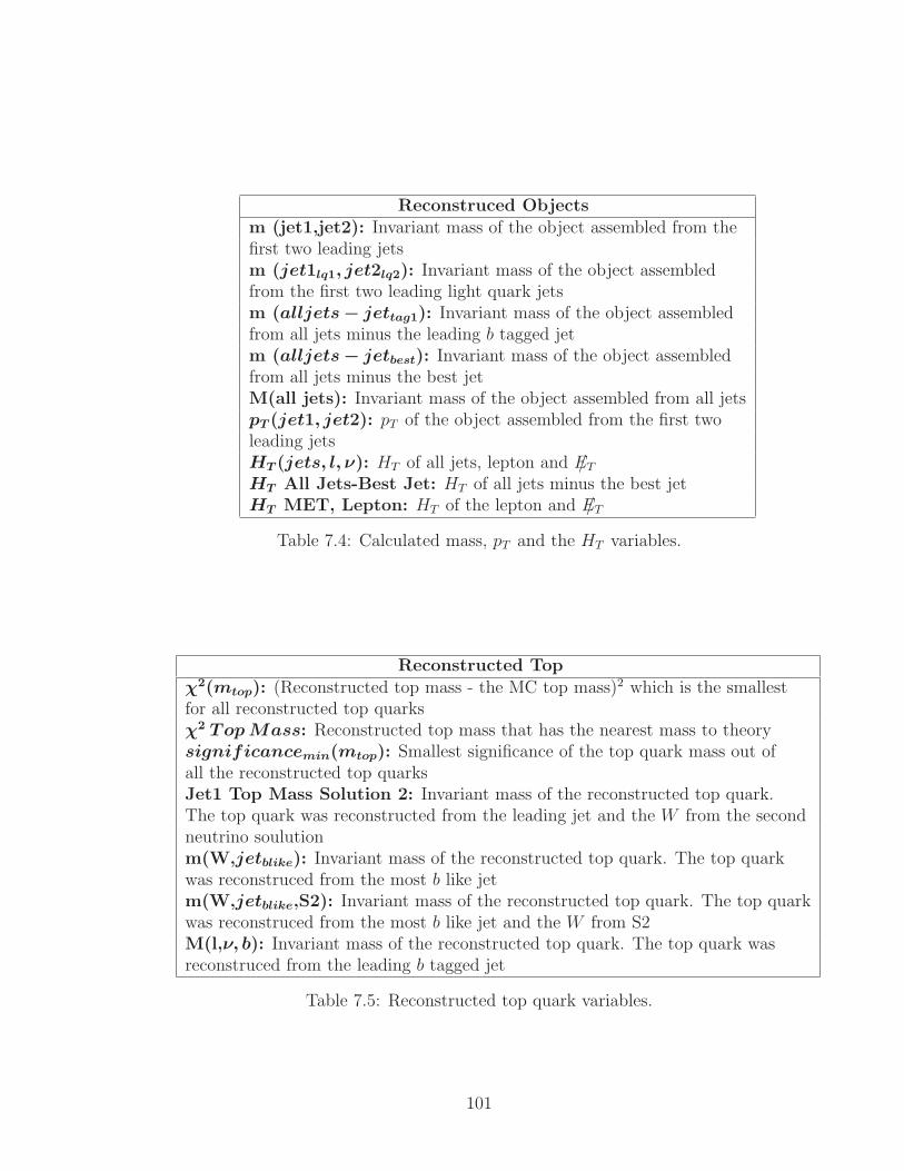
Reconstruced Objectsm (jet1,jet2): Invariant mass of the object assembled from thefirst two leading jetsm (jet1lq1, jet2lq2): Invariant mass of the object assembledfrom the first two leading light quark jetsm (alljets− jettag1): Invariant mass of the object assembledfrom all jets minus the leading b tagged jetm (alljets− jetbest): Invariant mass of the object assembledfrom all jets minus the best jetM(all jets): Invariant mass of the object assembled from all jetspT (jet1, jet2): pT of the object assembled from the first twoleading jetsHT (jets, l, ν): HT of all jets, lepton and /ET
HT All Jets-Best Jet: HT of all jets minus the best jetHT MET, Lepton: HT of the lepton and /ET
Table 7.4: Calculated mass, pT and the HT variables.
Reconstructed Topχ2(mtop): (Reconstructed top mass - the MC top mass)2 which is the smallestfor all reconstructed top quarksχ2 TopMass: Reconstructed top mass that has the nearest mass to theorysignificancemin(mtop): Smallest significance of the top quark mass out ofall the reconstructed top quarksJet1 Top Mass Solution 2: Invariant mass of the reconstructed top quark.The top quark was reconstructed from the leading jet and the W from the secondneutrino soulutionm(W,jetblike): Invariant mass of the reconstructed top quark. The top quarkwas reconstruced from the most b like jetm(W,jetblike,S2): Invariant mass of the reconstructed top quark. The top quarkwas reconstruced from the most b like jet and the W from S2M(l,ν, b): Invariant mass of the reconstructed top quark. The top quark wasreconstruced from the leading b tagged jet
Table 7.5: Reconstructed top quark variables.
101

Reconstructed W
Shericity (W, all jets): Shericity of all jets and the WAplanarity (all jets, W): Aplanarity of all jets and the WpT (W ): pT of the reconstructed WMT (W ): Transverse mass of the reconstructed W were mt = m2 + p2x + p2y
Table 7.6: Reconstructed W boson variables.
Angular CorrelationsDelta R all jets: minimum ∆R between any two jetsDelta φ Lepton MET: ∆φ between the lepton and /ET
Delta φ: ∆φ between jet2 and /ET
Most B like jet Delta φ: ∆φ between lepton and the most b like jetcos Best Lepton in CMF B-Tag: Cosine between the lepton in the b tagged topframe and the b tagged top in the center of mass frame. Here the b taggedtop is assembled from the leading b tagged jetcos Best Lepton in CMF: Cosine between the lepton in the best top frame and thebest top in the center of mass frame. Here the b tagged top is assembled from theleading b tagged jetcos Light quark Jet B-Tag: Cosine between the leading light quark jet and thelepton in b tagged top framecos(tag1,lepton)btaggedtop: Cosine between the leading tagged jet and the lepton inthe b tagged top framecos Lepton, Q×Z Best top: Cosine between the lepton and the z axis×Q(lepton)in the best top frame
Table 7.7: Angular Correlations.
102
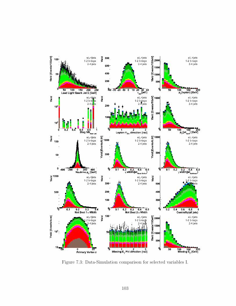
Figure 7.3: Data-Simulation comparison for selected variables I.
103

Figure 7.4: Data-Simulation comparison for selected variables II.
104
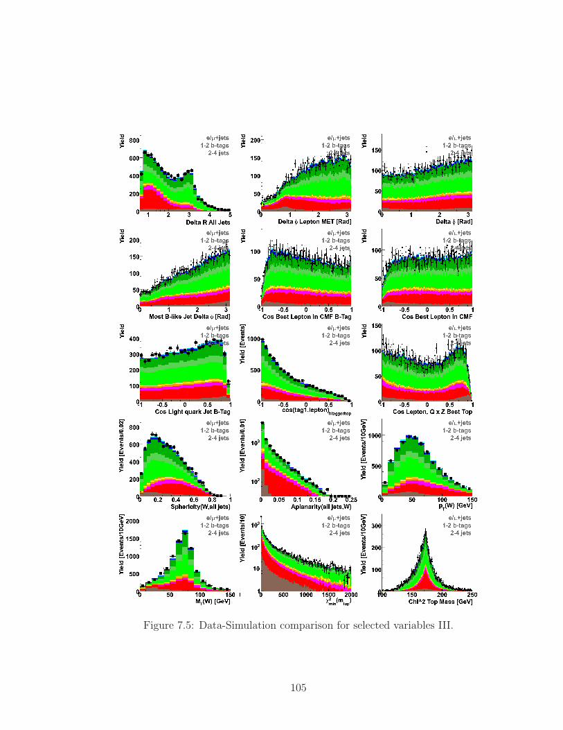
Figure 7.5: Data-Simulation comparison for selected variables III.
105
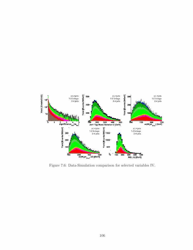
Figure 7.6: Data-Simulation comparison for selected variables IV.
106
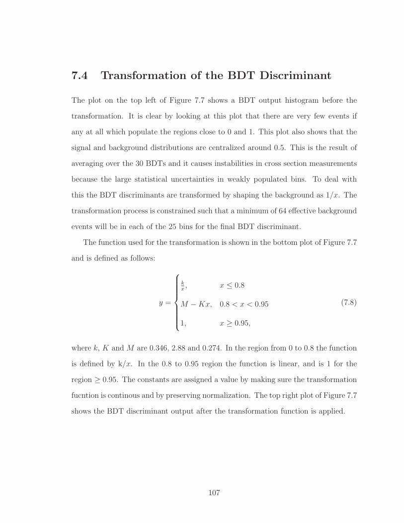
7.4 Transformation of the BDT Discriminant
The plot on the top left of Figure 7.7 shows a BDT output histogram before the
transformation. It is clear by looking at this plot that there are very few events if
any at all which populate the regions close to 0 and 1. This plot also shows that the
signal and background distributions are centralized around 0.5. This is the result of
averaging over the 30 BDTs and it causes instabilities in cross section measurements
because the large statistical uncertainties in weakly populated bins. To deal with
this the BDT discriminants are transformed by shaping the background as 1/x. The
transformation process is constrained such that a minimum of 64 effective background
events will be in each of the 25 bins for the final BDT discriminant.
The function used for the transformation is shown in the bottom plot of Figure 7.7
and is defined as follows:
y =
kx, x ≤ 0.8
M −Kx, 0.8 < x < 0.95
1, x ≥ 0.95,
(7.8)
where k, K and M are 0.346, 2.88 and 0.274. In the region from 0 to 0.8 the function
is defined by k/x. In the 0.8 to 0.95 region the function is linear, and is 1 for the
region ≥ 0.95. The constants are assigned a value by making sure the transformation
fucntion is continous and by preserving normalization. The top right plot of Figure 7.7
shows the BDT discriminant output after the transformation function is applied.
107
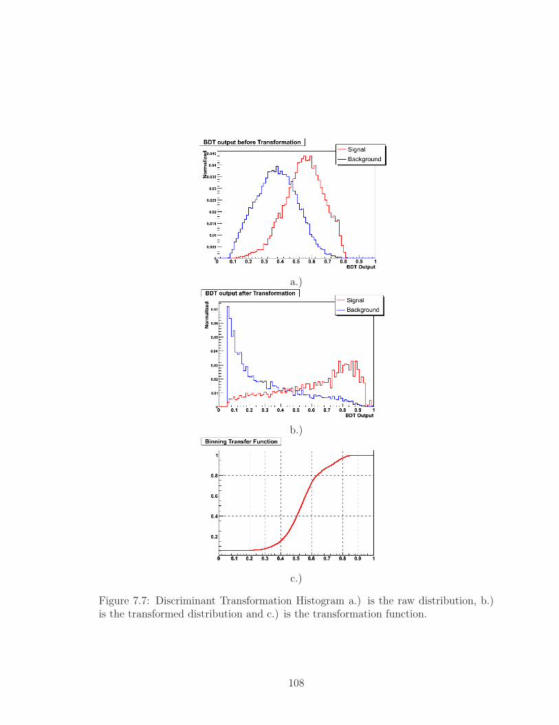
a.)
b.)
c.)
Figure 7.7: Discriminant Transformation Histogram a.) is the raw distribution, b.)is the transformed distribution and c.) is the transformation function.
108

7.5 Background Cross Checks
Two cross check samples are created for this analysis in order to check the modelling
of the background. This is done for the W+Jets and tt backgrounds. To ensure that
the discriminant outputs are dominated by these contributions additional selection
cuts are added. For the W+Jets check, HT < 175 GeV cut is applied and only events
with two jets are considered. For the tt check, a HT > 300 GeV cut is applied and
only events with four jets are considered. Figures 7.8 and 7.9 shows cross checks for
the s+t, s and t channel analyses. The first two rows are the cross checks for s+t, the
second two for s and the last two for t. Red indicates the tt contribution and green
indicates the W+Jets contribution. The last column for all three channels represent
the first two columns combined. These plots show good agreement between data and
simulation ensuring that the two main background for this analysis are well modeled.
109

tbtqb DT output0 0.2 0.4 0.6 0.8 1
Eve
nt Y
ield
0
10
20
30
40
-channelµe+1 b-tag
4 jets
tbtqb DT output0 0.2 0.4 0.6 0.8 1
Eve
nt Y
ield
0
10
20
30
40
tbtqb DT output0 0.2 0.4 0.6 0.8 1
Eve
nt Y
ield
0
10
20
30-channelµe+2 b-tags
4 jets
tbtqb DT output0 0.2 0.4 0.6 0.8 1
Eve
nt Y
ield
0
10
20
30
tbtqb DT output0 0.2 0.4 0.6 0.8 1
Eve
nt Y
ield
0
20
40
60
-channelµe+1-2 tags
4 jets
tbtqb DT output0 0.2 0.4 0.6 0.8 1
Eve
nt Y
ield
0
20
40
60
tbtqb DT output0 0.2 0.4 0.6 0.8 1
Eve
nt Y
ield
0
100
200
300
-channelµe+1 b-tag
2 jets
tbtqb DT output0 0.2 0.4 0.6 0.8 1
Eve
nt Y
ield
0
100
200
300
tbtqb DT output0 0.2 0.4 0.6 0.8 1
Eve
nt Y
ield
0
10
20
-channelµe+2 b-tags
2 jets
tbtqb DT output0 0.2 0.4 0.6 0.8 1
Eve
nt Y
ield
0
10
20
tbtqb DT output0 0.2 0.4 0.6 0.8 1
Eve
nt Y
ield
0
100
200
300
-channelµe+1-2 tags
2 jets
tbtqb DT output0 0.2 0.4 0.6 0.8 1
Eve
nt Y
ield
0
100
200
300
tb DT output0 0.2 0.4 0.6 0.8 1
Eve
nt Y
ield
0
20
40
60-channelµe+
1 b-tag 4 jets
tb DT output0 0.2 0.4 0.6 0.8 1
Eve
nt Y
ield
0
20
40
60
tb DT output0 0.2 0.4 0.6 0.8 1
Eve
nt Y
ield
0
10
20
30
40 -channelµe+2 b-tags
4 jets
tb DT output0 0.2 0.4 0.6 0.8 1
Eve
nt Y
ield
0
10
20
30
40
tb DT output0 0.2 0.4 0.6 0.8 1
Eve
nt Y
ield
0
20
40
60
-channelµe+1-2 tags
4 jets
tb DT output0 0.2 0.4 0.6 0.8 1
Eve
nt Y
ield
0
20
40
60
Figure 7.8: BDT cross check samples for s+t, s and t where the histograms dominatedby red correspond to tt events and the green dominated ones indicate W+Jet events.
110
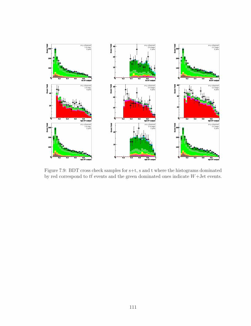
tb DT output0 0.2 0.4 0.6 0.8 1
Eve
nt Y
ield
0
100
200
300
-channelµe+1 b-tag
2 jets
tb DT output0 0.2 0.4 0.6 0.8 1
Eve
nt Y
ield
0
100
200
300
tb DT output0 0.2 0.4 0.6 0.8 1
Eve
nt Y
ield
0
10
20
30-channelµe+2 b-tags
2 jets
tb DT output0 0.2 0.4 0.6 0.8 1
Eve
nt Y
ield
0
10
20
30
tb DT output0 0.2 0.4 0.6 0.8 1
Eve
nt Y
ield
0
100
200
300
-channelµe+1-2 tags
2 jets
tb DT output0 0.2 0.4 0.6 0.8 1
Eve
nt Y
ield
0
100
200
300
tqb DT output0 0.2 0.4 0.6 0.8 1
Eve
nt Y
ield
0
20
40
-channelµe+1 b-tag
4 jets
tqb DT output0 0.2 0.4 0.6 0.8 1
Eve
nt Y
ield
0
20
40
tqb DT output0 0.2 0.4 0.6 0.8 1
Eve
nt Y
ield
0
10
20
30-channelµe+2 b-tags
4 jets
tqb DT output0 0.2 0.4 0.6 0.8 1
Eve
nt Y
ield
0
10
20
30
tqb DT output0 0.2 0.4 0.6 0.8 1
Eve
nt Y
ield
0
20
40
60 -channelµe+1-2 tags
4 jets
tqb DT output0 0.2 0.4 0.6 0.8 1
Eve
nt Y
ield
0
20
40
60
tqb DT output0 0.2 0.4 0.6 0.8 1
Eve
nt Y
ield
0
100
200
300
-channelµe+1 b-tag
2 jets
tqb DT output0 0.2 0.4 0.6 0.8 1
Eve
nt Y
ield
0
100
200
300
tqb DT output0 0.2 0.4 0.6 0.8 1
Eve
nt Y
ield
0
10
20
-channelµe+2 b-tags
2 jets
tqb DT output0 0.2 0.4 0.6 0.8 1
Eve
nt Y
ield
0
10
20
tqb DT output0 0.2 0.4 0.6 0.8 1
Eve
nt Y
ield
0
100
200
300
-channelµe+1-2 tags
2 jets
tqb DT output0 0.2 0.4 0.6 0.8 1
Eve
nt Y
ield
0
100
200
300
Figure 7.9: BDT cross check samples for s+t, s and t where the histograms dominatedby red correspond to tt events and the green dominated ones indicate W+Jet events.
111

Chapter 8
Analysis
This chapter gives an overview of this analysis starting with a discussion of how the
cross section measurements are made. This is followed by a discussion of systematic
uncertainties, results, significance and ends with measurement of the CKM matrix
element |Vtb|.
8.1 Cross Section Measurment
The measurement of the single top production cross sections is calculated using the
sets of six BDT discriminant outputs for each of the s channel, the t channel (see
Appendix A). For example, for the s+t channel analysis we use six BDT outputs, each
of which contains a 25 bin histogram giving a total of 150 independent s+ t channel
measurements. All of the cross section measurements and uncertainties are calculated
using the top statistics package [82, 83]. This employs both the fequentist and
bayesian approach, however for this analysis the latter is used. The package is also
used to validate the results which will be discussed in Section 8.3.
112

8.1.1 Bayesian Approach
In order to make a cross section measurement using the bayesian approach we initially
calculate the mean count d of both signal and background together. This is done for
each individual bin and defined by:
d = s+ b = αL σ +N∑
i=1
bi ≡ aσ +N∑
i=1
bi , (8.1)
where signal s = αLσ. Here α is the signal acceptance, L is the integrated luminosity,
σ is the cross section for the signal and a is defined as the effective luminosity αL.
The next step is to calculate the likelihood of observing a count D given the mean
count d. This is done using a Poisson distribution where the likelihood in each bin is
defined as:
L(D|d) = e−d dD
Γ(D + 1), (8.2)
where Γ is a Gamma function and is equal to D! when dealing with integer counts
of D as is the case for data. Since we are dealing with 150 bins we can build a total
likelihood by considering all bins as a product of each of the binned likelihoods:
L( ~D|~d) ≡ L( ~D|σ,~a,~b) =150∏
j=1
L(Dj|dj) , (8.3)
where ~D represents the vector for observed counts, ~d the vector for mean counts, and
~a and ~b the vectors for the effective luminosity and background.
The next step in the measurement is to use Baye’s theorem to calculate the pos-
terior probability density p(σ,~a,~b| ~D). This is done by integrating over vectors ~a and
113

~b to get the cross section posterior density given ~D which can be expressed as:
p(σ| ~D) =1
N
∫ ∫
L( ~D|σ,~a,~b)π(σ,~a,~b) d~a d~b . (8.4)
where the normalization constant N is calculated from∫ σmax
0p(σ| ~D)dσ = 1. The
prior probability density function is given by π(σ,~a,~b) and contains within it all the
information pertaining to σ, ~a and ~b. This information consists of the cross section,
yields for ~a and~b an all correlated systematic uncertainties. Since it is assumed that ~a
and~b are independent of σ we can then factorize the prior probability density function
as:
π(σ,~a,~b) = π(~a,~b)π(σ). (8.5)
By assuming π(σ) to be flat in σ, where:
π(σ) =1
σmax
, 0 < σ < σmax (8.6)
= 0, otherwise,
we avoid any potential bias towards a preferred cross section. Equation 8.4 can then
be rewritten as:
p(σ| ~D) =1
Nσmax
∫ ∫
L( ~D|σ,~a,~b)π(~a,~b) d~a d~b . (8.7)
In order to extract a cross section from p(σ| ~D) we plot p(σ| ~D) versus the cross section
and take the cross section as the mode (peak) of the curve shown in Figure 8.1
114
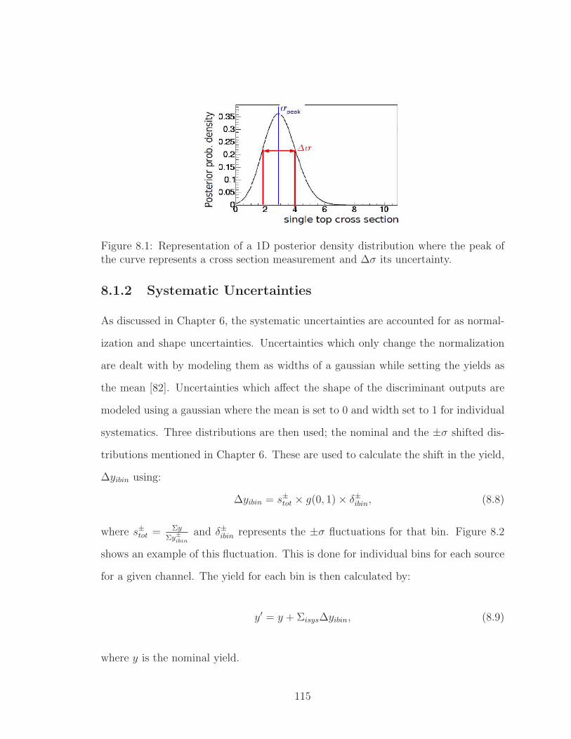
Figure 8.1: Representation of a 1D posterior density distribution where the peak ofthe curve represents a cross section measurement and ∆σ its uncertainty.
8.1.2 Systematic Uncertainties
As discussed in Chapter 6, the systematic uncertainties are accounted for as normal-
ization and shape uncertainties. Uncertainties which only change the normalization
are dealt with by modeling them as widths of a gaussian while setting the yields as
the mean [82]. Uncertainties which affect the shape of the discriminant outputs are
modeled using a gaussian where the mean is set to 0 and width set to 1 for individual
systematics. Three distributions are then used; the nominal and the ±σ shifted dis-
tributions mentioned in Chapter 6. These are used to calculate the shift in the yield,
∆yibin using:
∆yibin = s±tot × g(0, 1)× δ±ibin, (8.8)
where s±tot =Σy
Σy±ibin
and δ±ibin represents the ±σ fluctuations for that bin. Figure 8.2
shows an example of this fluctuation. This is done for individual bins for each source
for a given channel. The yield for each bin is then calculated by:
y′ = y + Σisys∆yibin, (8.9)
where y is the nominal yield.
115
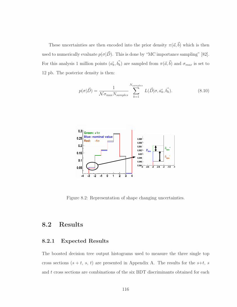
These uncertainties are then encoded into the prior density π(~a,~b) which is then
used to numerically evaluate p(σ| ~D). This is done by “MC importance sampling” [82].
For this analysis 1 million points ( ~ak, ~bk) are sampled from π(~a,~b) and σmax is set to
12 pb. The posterior density is then:
p(σ| ~D) =1
NσmaxNsamples
Nsamples∑
k=1
L( ~D|σ, ~ak, ~bk). (8.10)
Figure 8.2: Representation of shape changing uncertainties.
8.2 Results
8.2.1 Expected Results
The boosted decision tree output histograms used to measure the three single top
cross sections (s + t, s, t) are presented in Appendix A. The results for the s+t, s
and t cross sections are combinations of the six BDT discriminants obtained for each
116
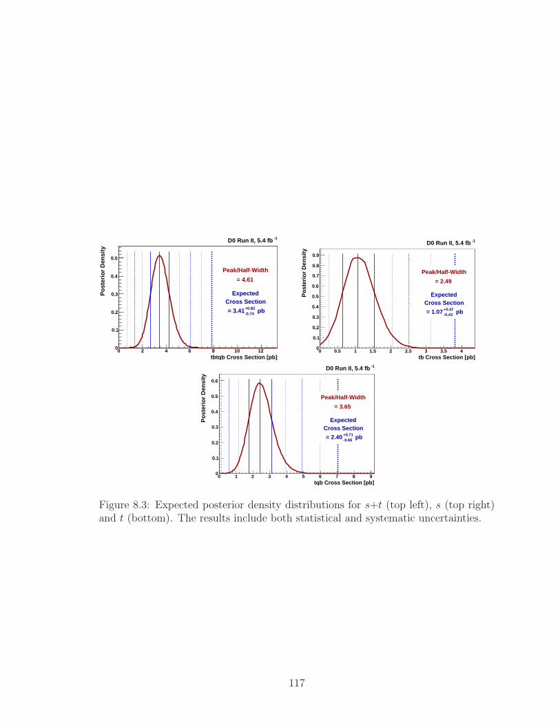
tbtqb Cross Section [pb]0 2 4 6 8 10 12
Pos
terio
r D
ensi
ty
0
0.1
0.2
0.3
0.4
0.5
-1D0 Run II, 5.4 fb
Peak/Half-Width
= 4.61
ExpectedCross Section
pb -0.74 +0.82 = 3.41
tb Cross Section [pb]0 0.5 1 1.5 2 2.5 3 3.5 4
Pos
terio
r D
ensi
ty
0
0.1
0.2
0.3
0.4
0.5
0.6
0.7
0.8
0.9
-1D0 Run II, 5.4 fb
Peak/Half-Width
= 2.49
ExpectedCross Section
pb -0.43 +0.47 = 1.07
tqb Cross Section [pb]0 1 2 3 4 5 6 7 8 9
Pos
terio
r D
ensi
ty
0
0.1
0.2
0.3
0.4
0.5
0.6
-1D0 Run II, 5.4 fb
Peak/Half-Width
= 3.65
ExpectedCross Section
pb -0.66 +0.71 = 2.40
Figure 8.3: Expected posterior density distributions for s+t (top left), s (top right)and t (bottom). The results include both statistical and systematic uncertainties.
117

cross section. The term expected refers to using only the MC signal and background
samples to make a cross section measurement. These measurements are done initially
so as not to bias subsequent measurements using the data. This also allows the
trouble shooting of unstable results and the optimization of the sensitivity in the
expected results. If the expected and observed results are consistent, this provieds
some confidence in the validity of the observed measurements.
The expected cross section results are shown in Table 8.1 and they are found to be
in good agreement with the SM values of 3.30 pb (s+t-channel), 1.04 pb (s-channel)
and 2.26 pb (t-channel). The corresponding bayesian posteriors are shown in Fig 8.3
for each cross section and the “peak over half-widths” are shown in Table 8.2. The
aim of these values is to provide an estimate of the sensitivity of the measurement.
Table 8.3 shows all the cross section measurements for the six individual channels.
In comparing the uncertainties of Tables 8.1 to 8.3 it is clear that by combining the
channels the uncertainty is reduced. The measurements for all individual channels
are presented in Table 8.3.
s+t-channel (pb) s-channel (pb) t-channel (pb)3.41+0.82
−0.74 1.07+0.47−0.43 2.40+0.71
−0.66
Table 8.1: Expected cross sections for s+t, s and t channels in pb.
s+t-channel s-channel t-channel4.61 2.49 3.65
Table 8.2: Expected posterior peak over half-width ratios for s+t, s and t channels.
8.2.2 Observed Results
This section presents the final cross section measurements obtained from the 5.4
fb−1dataset. All observed BDT discriminant outputs are shown in Appendix A.
118
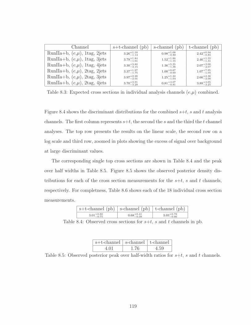
Channel s+t-channel (pb) s-channel (pb) t-channel (pb)RunIIa+b, (e,µ), 1tag, 2jets 3.26+1.18
−1.14 0.98+1.08−0.89 2.42+0.94
−0.85
RunIIa+b, (e,µ), 1tag, 3jets 3.79+1.84−1.61 1.52+1.86
−1.55 2.46+1.55−1.31
RunIIa+b, (e,µ), 1tag, 4jets 3.30+3.80−3.15 1.36+5.35
−1.36 2.07+3.00−2.07
RunIIa+b, (e,µ), 2tag, 2jets 3.37+1.97−1.75 1.00+0.67
−0.60 1.07+7.95−1.05
RunIIa+b, (e,µ), 2tag, 3jets 3.97+2.28−2.01 1.25+1.22
−1.04 2.66+2.36−2.00
RunIIa+b, (e,µ), 2tag, 4jets 3.70+3.91−3.29 0.81+4.07
−0.81 3.88+4.05−3.25
Table 8.3: Expected cross sections in individual analysis channels (e,µ) combined.
Figure 8.4 shows the discriminant distributions for the combined s+t, s and t analysis
channels. The first column represents s+t, the second the s and the third the t channel
analyses. The top row presents the results on the linear scale, the second row on a
log scale and third row, zoomed in plots showing the excess of signal over background
at large discriminant values.
The corresponding single top cross sections are shown in Table 8.4 and the peak
over half widths in Table 8.5. Figure 8.5 shows the observed posterior density dis-
tributions for each of the cross section measurements for the s+t, s and t channels,
respectively. For completness, Table 8.6 shows each of the 18 individual cross section
measurements.
s+t-channel (pb) s-channel (pb) t-channel (pb)3.01+0.80
−0.75 0.68+0.41−0.39 3.03+0.78
−0.66
Table 8.4: Observed cross sections for s+t, s and t channels in pb.
s+t-channel s-channel t-channel4.01 1.76 4.59
Table 8.5: Observed posterior peak over half-width ratios for s+t, s and t channels.
119
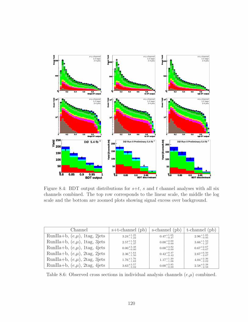
tbtqb DT output0 0.2 0.4 0.6 0.8 1
Eve
nt Y
ield
0
500
1000
-channelµe+1-2 tags2-4 jets
tbtqb DT output0 0.2 0.4 0.6 0.8 1
Eve
nt Y
ield
0
500
1000
tb DT output0 0.2 0.4 0.6 0.8 1
Eve
nt Y
ield
0
500
1000
-channelµe+1-2 tags2-4 jets
tb DT output0 0.2 0.4 0.6 0.8 1
Eve
nt Y
ield
0
500
1000
tqb DT output0 0.2 0.4 0.6 0.8 1
Eve
nt Y
ield
0
500
1000
-channelµe+1-2 tags2-4 jets
tqb DT output0 0.2 0.4 0.6 0.8 1
Eve
nt Y
ield
0
500
1000
tbtqb DT output0 0.2 0.4 0.6 0.8 1
Eve
nt Y
ield
210
310 -channelµe+1-2 tags2-4 jets
tbtqb DT output0 0.2 0.4 0.6 0.8 1
Eve
nt Y
ield
210
310
tb DT output0 0.2 0.4 0.6 0.8 1
Eve
nt Y
ield
210
310 -channelµe+1-2 tags2-4 jets
tb DT output0 0.2 0.4 0.6 0.8 1
Eve
nt Y
ield
210
310
tqb DT output0 0.2 0.4 0.6 0.8 1
Eve
nt Y
ield
210
310 -channelµe+1-2 tags2-4 jets
tqb DT output0 0.2 0.4 0.6 0.8 1
Eve
nt Y
ield
210
310
BDT output0.8 0.85 0.9 0.95 1
Yie
ld
0
50
100
150
200
250 -1DØ 5.4 fb
BDT output0.8 0.85 0.9 0.95 1
Yie
ld
0
50
100
150
200
250
BDT discriminant0.8 0.85 0.9 0.95 1
Yie
ld [E
vent
s/0.
04]
0
50
100
150
200 -1DØ Run II Preliminary 5.4 fb
BDT discriminant0.8 0.85 0.9 0.95 1
Yie
ld [E
vent
s/0.
04]
0
50
100
150
200
BDT discriminant0.8 0.85 0.9 0.95 1
Yie
ld [E
vent
s/0.
04]
0
50
100
150
200
-1DØ Run II Preliminary 5.4 fb
BDT discriminant0.8 0.85 0.9 0.95 1
Yie
ld [E
vent
s/0.
04]
0
50
100
150
200
Figure 8.4: BDT output distributions for s+t, s and t channel analyses with all sixchannels combined. The top row corresponds to the linear scale, the middle the logscale and the bottom are zoomed plots showing signal excess over background.
Channel s+t-channel (pb) s-channel (pb) t-channel (pb)RunIIa+b, (e,µ), 1tag, 2jets 3.24+1.25
−1.22 0.47+1.05−0.47 2.96+1.05
−0.95
RunIIa+b, (e,µ), 1tag, 3jets 2.57+1.52−1.37 0.00+2.00
−0.00 3.66+1.53−1.27
RunIIa+b, (e,µ), 1tag, 4jets 0.00+3.48−0.00 0.00+4.82
−0.00 0.67+2.67−0.67
RunIIa+b, (e,µ), 2tag, 2jets 2.36+1.64−1.50 0.42+0.47
−0.42 2.67+6.50−2.67
RunIIa+b, (e,µ), 2tag, 3jets 1.76+1.76−1.62 1.17+1.20
−1.06 4.04+2.36−2.02
RunIIa+b, (e,µ), 2tag, 4jets 3.63+3.57−3.02 0.00+3.85
−0.00 2.58+3.38−2.58
Table 8.6: Observed cross sections in individual analysis channels (e,µ) combined.
120
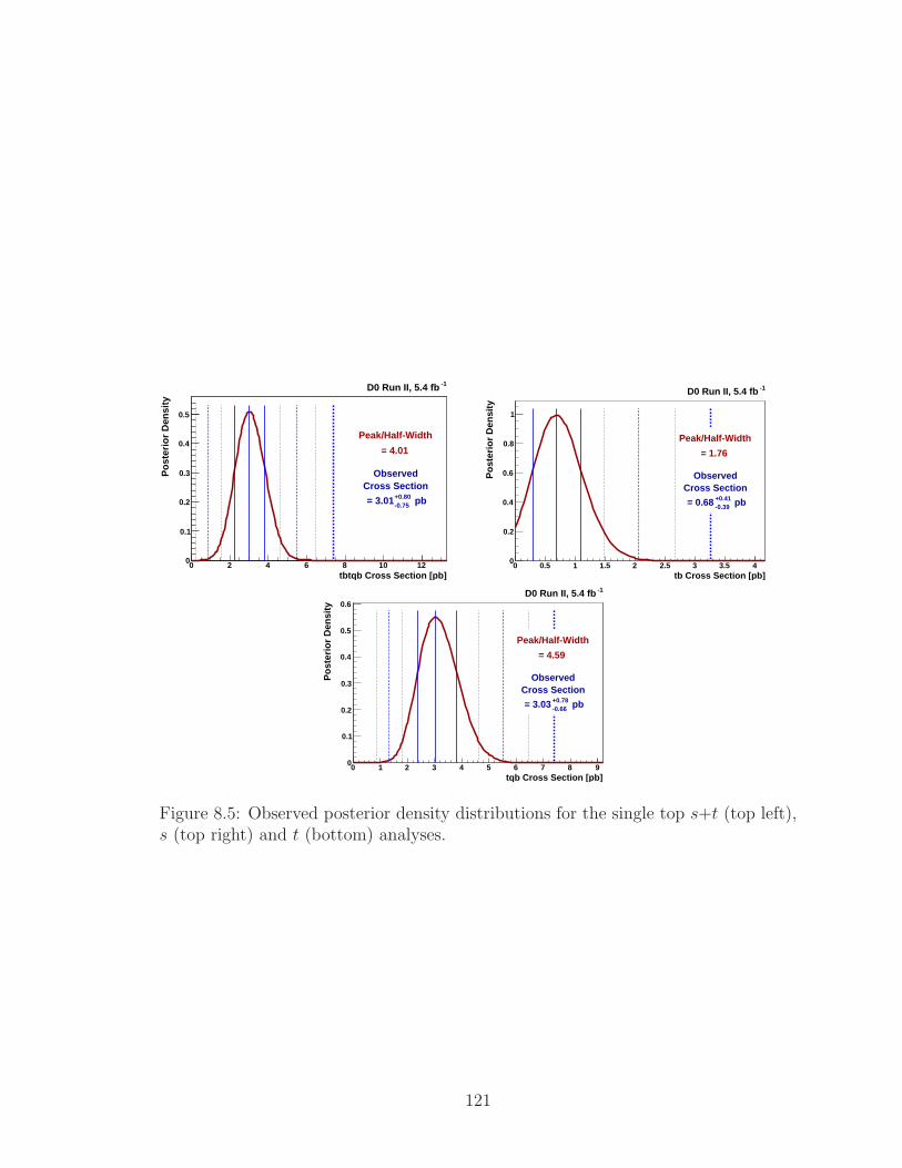
tbtqb Cross Section [pb]0 2 4 6 8 10 12
Pos
terio
r D
ensi
ty
0
0.1
0.2
0.3
0.4
0.5
-1D0 Run II, 5.4 fb
Peak/Half-Width
= 4.01
ObservedCross Section
pb -0.75 +0.80 = 3.01
tb Cross Section [pb]0 0.5 1 1.5 2 2.5 3 3.5 4
Pos
terio
r D
ensi
ty
0
0.2
0.4
0.6
0.8
1
-1D0 Run II, 5.4 fb
Peak/Half-Width
= 1.76
ObservedCross Section
pb -0.39 +0.41 = 0.68
tqb Cross Section [pb]0 1 2 3 4 5 6 7 8 9
Pos
terio
r D
ensi
ty
0
0.1
0.2
0.3
0.4
0.5
0.6
-1D0 Run II, 5.4 fb
Peak/Half-Width
= 4.59
ObservedCross Section
pb -0.66 +0.78 = 3.03
Figure 8.5: Observed posterior density distributions for the single top s+t (top left),s (top right) and t (bottom) analyses.
121
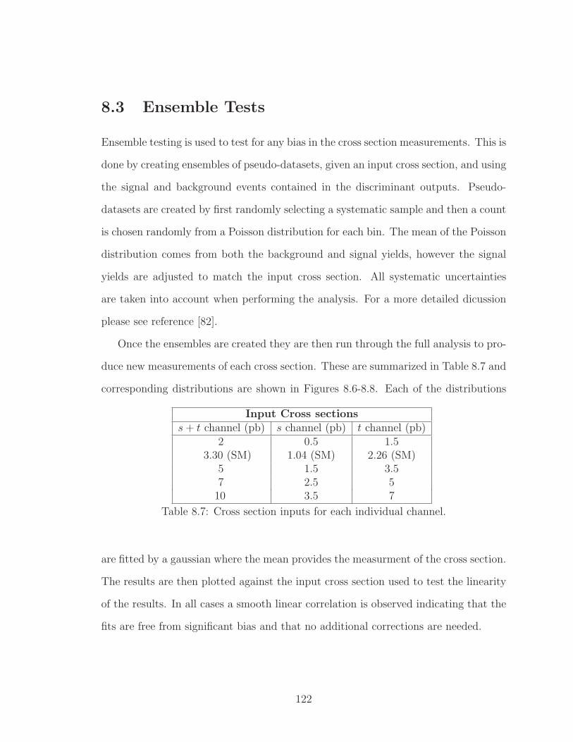
8.3 Ensemble Tests
Ensemble testing is used to test for any bias in the cross section measurements. This is
done by creating ensembles of pseudo-datasets, given an input cross section, and using
the signal and background events contained in the discriminant outputs. Pseudo-
datasets are created by first randomly selecting a systematic sample and then a count
is chosen randomly from a Poisson distribution for each bin. The mean of the Poisson
distribution comes from both the background and signal yields, however the signal
yields are adjusted to match the input cross section. All systematic uncertainties
are taken into account when performing the analysis. For a more detailed dicussion
please see reference [82].
Once the ensembles are created they are then run through the full analysis to pro-
duce new measurements of each cross section. These are summarized in Table 8.7 and
corresponding distributions are shown in Figures 8.6-8.8. Each of the distributions
Input Cross sectionss+ t channel (pb) s channel (pb) t channel (pb)
2 0.5 1.53.30 (SM) 1.04 (SM) 2.26 (SM)
5 1.5 3.57 2.5 510 3.5 7
Table 8.7: Cross section inputs for each individual channel.
are fitted by a gaussian where the mean provides the measurment of the cross section.
The results are then plotted against the input cross section used to test the linearity
of the results. In all cases a smooth linear correlation is observed indicating that the
fits are free from significant bias and that no additional corrections are needed.
122

LINEARITY TEST FOR BDT s+t CHANNEL
0 2 4 6 8 10 120
100
200
300
400
500
600
700
800
Measured cross section in ensembles full_ens_peakEntries 9250Mean 1.924RMS 0.7228
0.008±Mean: 1.935
Measured cross section in ensembles
0 2 4 6 8 10 120
100
200
300
400
500
600
700
800
Measured cross section in ensembles full_ens_peakEntries 10000Mean 3.214RMS 0.8008
0.008±Mean: 3.206
Measured cross section in ensembles
0 2 4 6 8 10 120
100
200
300
400
500
600
700
Measured cross section in ensembles full_ens_peakEntries 10000Mean 4.886RMS 0.8923
0.009±Mean: 4.885
Measured cross section in ensembles
0 2 4 6 8 10 12 14 16 18 200
200
400
600
800
1000
Measured cross section in ensembles full_ens_peakEntries 9750Mean 6.882RMS 1.023
0.010±Mean: 6.879
Measured cross section in ensembles
0 2 4 6 8 10 12 14 16 18 200
100
200
300
400
500
600
700
800
900
Measured cross section in ensembles full_ens_peakEntries 10000Mean 9.858RMS 1.271
0.013±Mean: 9.804
Measured cross section in ensembles
Input Single Top Cross Section [pb]0 2 4 6 8 10
Mea
sure
d S
ingl
e T
op C
ross
Sec
tion
[pb]
0
2
4
6
8
10
BDT Ensemble Linearity Test for s+t-channel
0.0017±Slope: 0.9857 0.0087±Intercept: -0.0396
uncertainty on the fit±Mean Values
68% CL
BDT Ensemble Linearity Test for s+t-channel
Figure 8.6: Results of ensemble tests for the combined s + t channel analysis. Theobserved linear behavior indicates the absence of bias from the analysis procedure.
123
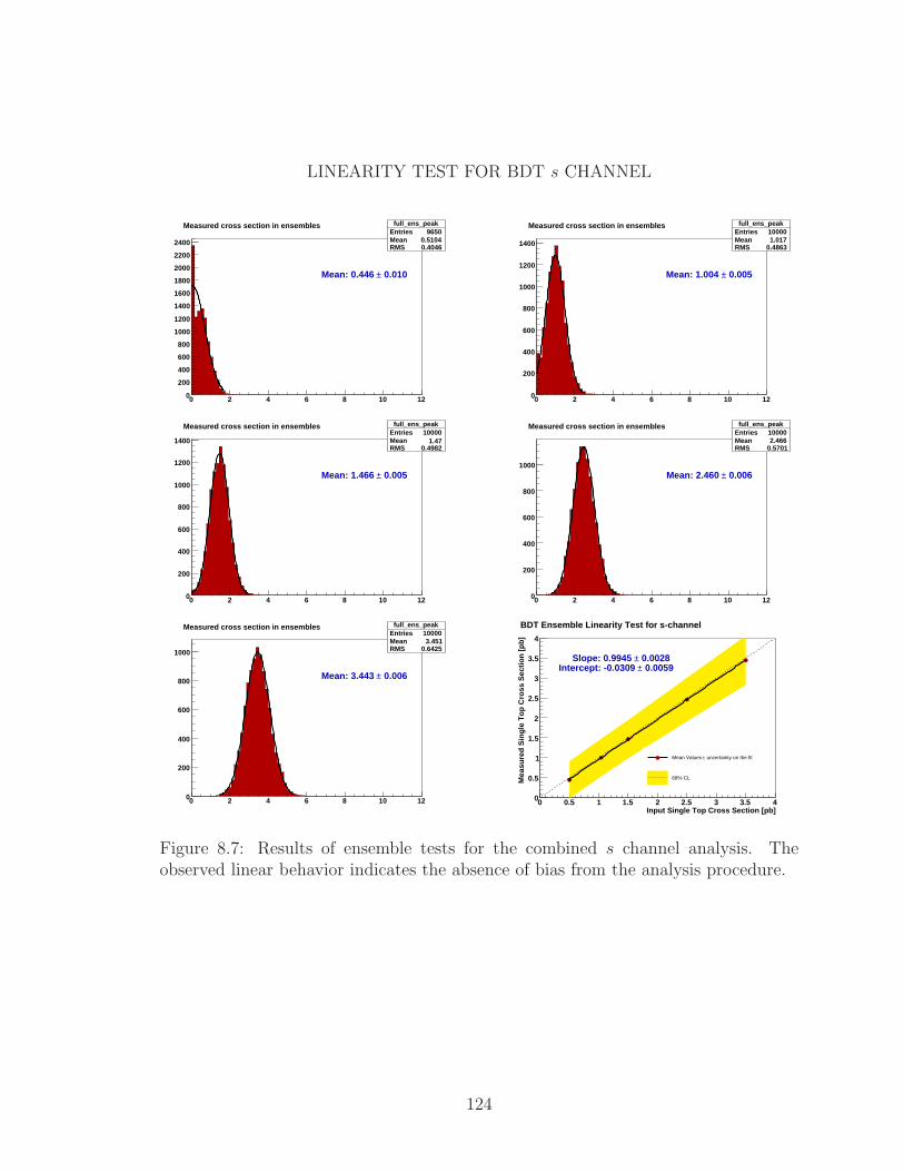
LINEARITY TEST FOR BDT s CHANNEL
0 2 4 6 8 10 120
200
400
600
800
1000
1200
1400
1600
1800
2000
2200
2400
Measured cross section in ensembles full_ens_peakEntries 9650Mean 0.5104RMS 0.4046
0.010±Mean: 0.446
Measured cross section in ensembles
0 2 4 6 8 10 120
200
400
600
800
1000
1200
1400
Measured cross section in ensembles full_ens_peakEntries 10000Mean 1.017RMS 0.4863
0.005±Mean: 1.004
Measured cross section in ensembles
0 2 4 6 8 10 120
200
400
600
800
1000
1200
1400
Measured cross section in ensembles full_ens_peakEntries 10000Mean 1.47RMS 0.4982
0.005±Mean: 1.466
Measured cross section in ensembles
0 2 4 6 8 10 120
200
400
600
800
1000
Measured cross section in ensembles full_ens_peakEntries 10000Mean 2.466RMS 0.5701
0.006±Mean: 2.460
Measured cross section in ensembles
0 2 4 6 8 10 120
200
400
600
800
1000
Measured cross section in ensembles full_ens_peakEntries 10000Mean 3.451RMS 0.6425
0.006±Mean: 3.443
Measured cross section in ensembles
Input Single Top Cross Section [pb]0 0.5 1 1.5 2 2.5 3 3.5 4
Mea
sure
d S
ingl
e T
op C
ross
Sec
tion
[pb]
0
0.5
1
1.5
2
2.5
3
3.5
4
BDT Ensemble Linearity Test for s-channel
0.0028±Slope: 0.9945 0.0059±Intercept: -0.0309
uncertainty on the fit±Mean Values
68% CL
BDT Ensemble Linearity Test for s-channel
Figure 8.7: Results of ensemble tests for the combined s channel analysis. Theobserved linear behavior indicates the absence of bias from the analysis procedure.
124

LINEARITY TEST FOR BDT t CHANNEL
0 2 4 6 8 10 120
200
400
600
800
1000
Measured cross section in ensembles full_ens_peakEntries 10150Mean 1.452RMS 0.6434
0.007±Mean: 1.453
Measured cross section in ensembles
0 2 4 6 8 10 120
200
400
600
800
1000
Measured cross section in ensembles full_ens_peakEntries 10100Mean 2.189RMS 0.7023
0.007±Mean: 2.188
Measured cross section in ensembles
0 2 4 6 8 10 120
100
200
300
400
500
600
700
800
Measured cross section in ensembles full_ens_peakEntries 10250Mean 3.426RMS 0.8145
0.008±Mean: 3.415
Measured cross section in ensembles
0 2 4 6 8 10 120
100
200
300
400
500
600
700
Measured cross section in ensembles full_ens_peakEntries 10000Mean 4.9RMS 0.9456
0.010±Mean: 4.902
Measured cross section in ensembles
0 2 4 6 8 10 12 14 16 18 200
100
200
300
400
500
600
700
800
Measured cross section in ensembles full_ens_peakEntries 8550Mean 6.876RMS 1.129
0.012±Mean: 6.867
Measured cross section in ensembles
Input Single Top Cross Section [pb]0 1 2 3 4 5 6 7 8
Mea
sure
d S
ingl
e T
op C
ross
Sec
tion
[pb]
0
1
2
3
4
5
6
7
8
BDT Ensemble Linearity Test for t-channel
0.0021±Slope: 0.9855 0.0076±Intercept: -0.0315
uncertainty on the fit±Mean Values
68% CL
BDT Ensemble Linearity Test for t-channel
Figure 8.8: Results of ensemble tests for the combined t channel analysis. The ob-served linear behavior indicates the absence of bias from the analysis procedure.
125
8.3.1 Significance
The statistical significance of a measurement is generally calculated by finding the
“p-value” of that measurement. The p-values from this analysis can be interpreted
as the probability of measuring a given cross section in data if the dataset contained
no single top events. Typically this is expressed in standard deviations where α
represents the p-value. The number of standard deviations is then given by
Nσ =√2erf−1(1− 2α). (8.11)
8.3.2 Asymptotic approximation of the log-likelihood ratio
In the previous DØ analysis, the cross section significance was calculated using en-
sembles of pseudo-datasets that contained no siganl [80]. This approach takes a large
amount of cpu time and translates to about a month of computing time. A more
effective approach called the log likelihood method channel analysis was used in the
t channel anlaysis [84, 86]. However, this too is very cpu intensive but less so than
ensemble testing. For this analysis the asymtotic approximation of the log-likelihood
method (AALR) has been used [86]. The results have been compared to the previous
analyses and are found to be consistent [53].
As stated earlier, the goal of measuring a significance is to obtain a p-value. In
the AALR method this is done by first defining the log-likelihood ratio
Q = −2 lnL(µ = 1)
L(µ = 0), (8.12)
where the likelihood is defined by L(µ). The likelihood includes all systematic for
σ = µσo, where µ is the strength parameter and σo the theoretical cross section for
126
the single top signal. The 1 represents the likelihood for a theoretical signal cross
section compared to the likelihood of no theoretical cross section (background only).
If a number of events are to be assesed by AALR given as signal strength of µ′
then the output distribution is a Gaussian whose mean and variance is
E[Q] = α2(1− 2µ′) (8.13)
V [Q] = 4α2, (8.14)
where α is defined as
α =
√
−2 ln LA(µ)LA(µ)
|µ− µ′| , (8.15)
and µ corresponds to the maximum value for the likelihood. Assuming that α is
independent of µ then we can then set µ′ = 0 and µ then becomes µexp = σexp/σo
where σexp is the expected cross section. This is the background only scenario where
the probability density ρ(Q) is given by a Gaussian with a mean and variance defined
as α2B and 4α2
B. For the signal plus background case the mean and variance become
−α2S+B and 4α2
S+B. In order to calculate the p-value we use the cumulative distribu-
tion for a Gaussian Φ with mean 0 and variance 1 for which the p-value is defined
as
p =
∫ Qobs
−∞ρ(Q)dQ = Φ
(
Qobs − α2
2α
)
. (8.16)
8.3.3 Measured Significance
Table 8.9 summarizes the parameters and significance calculations for s+t, s and t
channels analyses. Figs 8.9-8.11 show the expected and observed significances for
the three analyses. In each figure the green curve represents the background only
scenario and blue curve the signal plus background case. The position of the black
127
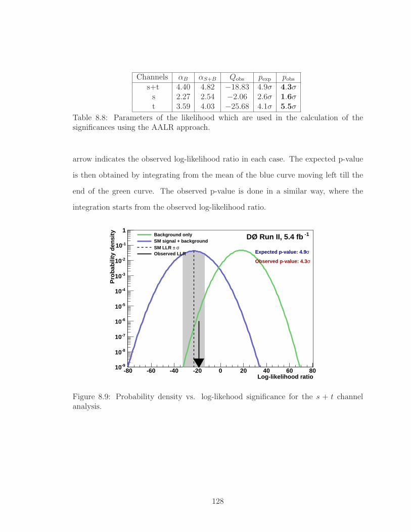
Channels αB αS+B Qobs pexp pobss+t 4.40 4.82 −18.83 4.9σ 4.3σs 2.27 2.54 −2.06 2.6σ 1.6σt 3.59 4.03 −25.68 4.1σ 5.5σ
Table 8.8: Parameters of the likelihood which are used in the calculation of thesignificances using the AALR approach.
arrow indicates the observed log-likelihood ratio in each case. The expected p-value
is then obtained by integrating from the mean of the blue curve moving left till the
end of the green curve. The observed p-value is done in a similar way, where the
integration starts from the observed log-likelihood ratio.
Log-likelihood ratio-80 -60 -40 -20 0 20 40 60 80
Pro
babi
lity
dens
ity
-910
-810
-710
-610
-510
-410
-310
-210
-110
1 -1DØ Run II, 5.4 fb
σExpected p-value: 4.9
σObserved p-value: 4.3
Background onlySM signal + background
σ ±SM LLR Observed LLR
Figure 8.9: Probability density vs. log-likehood significance for the s + t channelanalysis.
128

Log-likelihood ratio-80 -60 -40 -20 0 20 40 60 80
Pro
babi
lity
dens
ity
-910
-810
-710
-610
-510
-410
-310
-210
-110
1 -1DØ Run II, 5.4 fb
σExpected p-value: 2.6
σObserved p-value: 1.6
Background onlySM signal + background
σ ±SM LLR Observed LLR
Figure 8.10: Probability density vs. log-likehood significance for the s channel anal-ysis.
129
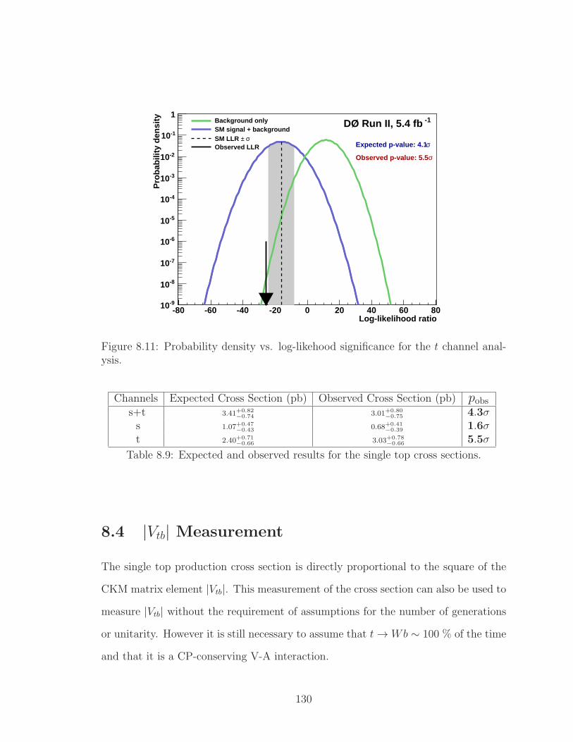
Log-likelihood ratio-80 -60 -40 -20 0 20 40 60 80
Pro
babi
lity
dens
ity
-910
-810
-710
-610
-510
-410
-310
-210
-110
1 -1DØ Run II, 5.4 fb
σExpected p-value: 4.1
σObserved p-value: 5.5
Background onlySM signal + background
σ ±SM LLR Observed LLR
Figure 8.11: Probability density vs. log-likehood significance for the t channel anal-ysis.
Channels Expected Cross Section (pb) Observed Cross Section (pb) pobss+t 3.41+0.82
−0.74 3.01+0.80−0.75 4.3σ
s 1.07+0.47−0.43 0.68+0.41
−0.39 1.6σt 2.40+0.71
−0.66 3.03+0.78−0.66 5.5σ
Table 8.9: Expected and observed results for the single top cross sections.
8.4 |Vtb| Measurement
The single top production cross section is directly proportional to the square of the
CKM matrix element |Vtb|. This measurement of the cross section can also be used to
measure |Vtb| without the requirement of assumptions for the number of generations
or unitarity. However it is still necessary to assume that t → Wb ∼ 100 % of the time
and that it is a CP-conserving V-A interaction.
130
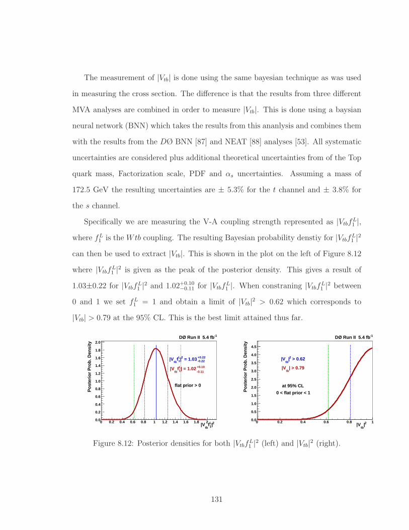
The measurement of |Vtb| is done using the same bayesian technique as was used
in measuring the cross section. The difference is that the results from three different
MVA analyses are combined in order to measure |Vtb|. This is done using a baysian
neural network (BNN) which takes the results from this ananlysis and combines them
with the results from the DØ BNN [87] and NEAT [88] analyses [53]. All systematic
uncertainties are considered plus additional theoretical uncertainties from of the Top
quark mass, Factorization scale, PDF and αs uncertainties. Assuming a mass of
172.5 GeV the resulting uncertainties are ± 5.3% for the t channel and ± 3.8% for
the s channel.
Specifically we are measuring the V-A coupling strength represented as |VtbfL1 |,
where fL1 is the Wtb coupling. The resulting Bayesian probability denstiy for |Vtbf
L1 |2
can then be used to extract |Vtb|. This is shown in the plot on the left of Figure 8.12
where |VtbfL1 |2 is given as the peak of the posterior density. This gives a result of
1.03±0.22 for |VtbfL1 |2 and 1.02+0.10
−0.11 for |VtbfL1 |. When constraning |Vtbf
L1 |2 between
0 and 1 we set fL1 = 1 and obtain a limit of |Vtb|2 > 0.62 which corresponds to
|Vtb| > 0.79 at the 95% CL. This is the best limit attained thus far.
2|1Lf
tb|V
0 0.2 0.4 0.6 0.8 1 1.2 1.4 1.6 1.8 2
Pos
terio
r P
rob.
Den
sity
0.0
0.2
0.4
0.6
0.8
1.0
1.2
1.4
1.6
1.8
2.0
-1DØ Run II 5.4 fb
-0.22 +0.22 = 1.032|1
Lftb
|V
-0.11
+0.10 | = 1.021Lf
tb|V
flat prior > 0
2|tb
|V0 0.2 0.4 0.6 0.8 1
Pos
terio
r P
rob.
Den
sity
0.0
0.5
1.0
1.5
2.0
2.5
3.0
3.5
4.0
4.5
-1DØ Run II 5.4 fb
> 0.622|tb
|V
| > 0.79tb
|V
at 95% CL
0 < flat prior < 1
Figure 8.12: Posterior densities for both |VtbfL1 |2 (left) and |Vtb|2 (right).
131
Chapter 9
Comparison of Results
9.1 DØ and CDF Measurements
In this chapter we compare results from DØ and CDF single top analyses and the
predictions of the NLO QCD. We also compare the result of this analysis with those
obtained from the previous (2009) DØ analyses [80]. The integrated luminosities for
these results are, 2.3fb−1 for (DØ 2009) [80], 5.4fb−1 for (this analysis) and 3.2fb−1
(CDF) [85].
The DØ single top group uses two different approaches to calculate cross sec-
tions. The first is the one dimensional approach which was discussed in Section 8.1.1.
This approach was used for the three MVA analyses: Boosted Decision Trees (this
analysis), Bayesian Neural Networks (BNN) and, Neural Evolution of Augmenting
Topologies (NEAT). Each MVA provides a cross section measurement for s+ t, s and
t channels. The results were combined using two different BNN methods. The first
used as input the results from the three sets of MVA results and is labelled BNN
Combination. The second, labelled BNN Combination 6, takes as input the s and
t measurements from the three MVA analyses, hence the number six. In both cases
132

the combined s+ t, s and t channel cross sections are measured.
The second method is a two dimensional approach. This is used specifically to
measure the separated s and t channel cross sections. It uses a two dimensional
posterior density function for the combined s and t channels. This is done without
making any assumption on the predicted cross sections. Using the 2D posterior
density we can then integrate over either s or t to obtain a 1D posterior density. This
is shown in Figure 9.3 for the BNN, which is labelled BNN Combination t method.
In this case the training was implemented so as to focus on the t channel. The BNN
Combination 6 method also uses the 2D approach and these results are compared to
the other methods in Fig 9.1. The significance values presented in Figures 9.1 and
9.2 are labelled 2D if the cross sections were obtained from the 2D method, otherwise
they are 1D measurements.
9.1.1 Comparisons
Fig 9.1 a) shows the comparison of the DØ results from the three different MVA
analyses and for the combinations for the combined s+ t-channel cross section. The
measurements are consistent within one sigma as well as being in agreement with the
predicted cross section of 3.30 ± 0.13 pb. Fig 9.1 b) shows the corresponding results
for the s channel and Fig 9.1 c), for the t channel. The results are all consistent
within one standard deviation. The s channel results are also consistent with the
predicted cross section (1.04 ± .04pb) at the one standard deviation level, apart from
the NEAT result, which is within 2 standard deviations. The t-channel results are
all consistent with theory (2.26 ± 0.12pb) and with eachother at the one standard
deviation level. Table 9.1 shows a list of significances for the three channels. The
results of note are the observed p-values for the t channel using BDTs (5.5σ), BNN
133

Combination t (5.5σ (2D)) and the s + t channel using BNN Combination 6 (5.6σ).
These are the best measurements for each of these channels.
Figure 9.2 compares these results with those from the previous DØ analysis and
with those from CDF. Good agreement is observed between the DØ results for the
s + t, s and t channels. The CDF combination is consistent within a 1-2 sigma
uncertainty and they tend to be less consistent with the theoretical predictions. The
significances of these results can be seen in Table 9.2.
134
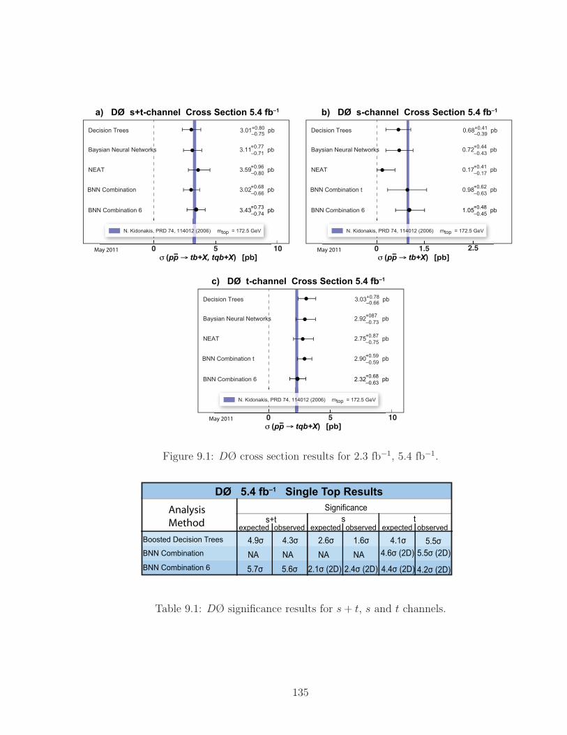
1050
σ (pp → tb+X, tqb+X) [pb]
N. Kidonakis, PRD 74, 114012 (2006) mtop = 172.5 GeV
BNN Combination 6 3.43+0.73
–0.74pb
BNN Combination 3.02+0.68
–0.66pb
NEAT 3.59+0.96
–0.80pb
Baysian Neural Networks 3.11+0.77
–0.71pb
Decision Trees 3.01+0.80–0.75
pb
May 2011
a) DØ s+t-channel Cross Section 5.4 fb–1
2.51.50
σ (pp → tb+X) [pb]
N. Kidonakis, PRD 74, 114012 (2006) mtop = 172.5 GeV
BNN Combination 6 1.05+0.48
–0.45pb
BNN Combination t 0.98+0.62
–0.63pb
NEAT 0.17+0.41
–0.17pb
Baysian Neural Networks 0.72+0.44
–0.43pb
Decision Trees 0.68+0.41–0.39
pb
May 2011
b) DØ s-channel Cross Section 5.4 fb–1
1050
σ (pp → tqb+X) [pb]
N. Kidonakis, PRD 74, 114012 (2006) mtop = 172.5 GeV
BNN Combination 6 2.32+0.68
–0.63pb
BNN Combination t 2.90+0.59
–0.59pb
NEAT 2.75+0.87
–0.75pb
Baysian Neural Networks 2.92+087
–0.73pb
Decision Trees 3.03+0.78–0.66
pb
May 2011
c) DØ t-channel Cross Section 5.4 fb–1
Figure 9.1: DØ cross section results for 2.3 fb−1, 5.4 fb−1.
DØ 5.4 fb–1 Single Top Results
Significance
s+t s texpected expected expectedobserved observed observed
Boosted Decision Trees
BNN Combination
BNN Combination 6
4.9σ
NA
5.7σ
4.3σ
NA
5.6σ
2.6σ
NA
2.1σ (2D)
1.6σ
NA
2.4σ (2D)
4.1σ
4.6σ (2D)
4.4σ (2D)
5.5σ
5.5σ (2D)
4.2σ (2D)
Analysis
Method
Table 9.1: DØ significance results for s+ t, s and t channels.
135
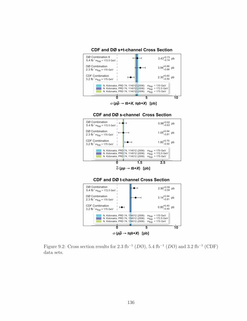
1050
σ (pp → tb+X, tqb+X) [pb]
50
N. Kidonakis, PRD 74, 114012 (2006) mtop = 172.5 GeV
N. Kidonakis, PRD 74, 114012 (2006) mtop = 175 GeV
N. Kidonakis, PRD 74, 114012 (2006) mtop = 170 GeV
CDF Combination3.2 fb
–1 mtop = 175 GeV
2.30+0.60
–0.50pb
DØ Combination2.3 fb
–1 mtop = 170 GeV
3.94+0.88
–0.88pb
DØ Combination 6 5.4 fb
–1 mtop = 172.5 GeV
3.43+0.73–0.74
pb
CDF and DØ s+t-channel Cross Section
2.51.50
σ (pp → tb+X) [pb]
2 51 50
N. Kidonakis, PRD 74, 114012 (2006) mtop = 172.5 GeV
N. Kidonakis, PRD 74, 114012 (2006) mtop = 175 GeV
N. Kidonakis, PRD 74, 114012 (2006) mtop = 170 GeV
CDF Combination3.2 fb
–1 mtop = 175 GeV
1.80+0.70
–0.50pb
DØ Combination2.3 fb
–1 mtop = 170 GeV
1.05+0.94
–0.81pb
DØ Combination 5.4 fb
–1 mtop = 172.5 GeV
0.98+0.62–0.63
pb
CDF and DØ s-channel Cross Section
1050
σ (pp → tqb+X) [pb]
50
N. Kidonakis, PRD 74, 114012 (2006) mtop = 172.5 GeV
N. Kidonakis, PRD 74, 114012 (2006) mtop = 175 GeV
N. Kidonakis, PRD 74, 114012 (2006) mtop = 170 GeV
CDF Combination3.2 fb
–1 mtop = 175 GeV
0.80+0.40
–0.40pb
DØ Combination2.3 fb
–1 mtop = 170 GeV
3.14+0.94
–0.81pb
DØ Combination 5.4 fb
–1 mtop = 172.5 GeV
2.90+0.59–0.59
pb
CDF and DØ t-channel Cross Section
Figure 9.2: Cross section results for 2.3 fb−1 (DØ), 5.4 fb−1 (DØ) and 3.2 fb−1 (CDF)data sets.
136

DØ and CDF Combination Single Top Results
Significances+t s t
expected expected expectedobserved observed observed
DØ 5.4 fb-1
DØ Comb6 5.4 fb-1
DØ 2.3 fb-1
NA
5.7σ
4.5σ
NA
5.6σ
5.0σ
2.7σ
2.1σ (2D)
NA
1.8σ
2.4σ (2D)
NA
4.6σ (2D)
4.4σ (2D)
3.7σ
5.5σ (2D)
4.2σ (2D)
4.8σ
Analysis
Method
CDF 3.2 fb-1 5.9σ 5.0σ NA NA NA NA
Table 9.2: DØ and CDF significance results for s+ t, s and t channels.
137

s-channel cross section [pb]0 2 4
t-ch
anne
l cro
ss s
ectio
n [p
b]
0
2
4
Measurement [1]
SM[2]Four generations
[3]Top-flavor
[4]FCNC
68% C.L.90% C.L.95% C.L.
s-channel cross section [pb]0 2 4
t-ch
anne
l cro
ss s
ectio
n [p
b]
0
2
4
[1] PRD 74: 114012, 2006[2] EPJ C49: 791, 2007[3] PRD 63: 014018, 2001[4] PRL 99: 191802, 2007
-1DØ 5.4 fb
s-channel cross section [pb]0 0.5 1 1.5 2 2.5 3
Pos
terio
r de
nsity
0
0.1
0.2
0.3
0.4
0.5
0.6
0.7 -1DØ Run II, 5.4 fb
Peak/Half-Width
= 1.56
ObservedCross Section
pb -0.63 +0.62 = 0.98
s-channel cross section [pb]0 0.5 1 1.5 2 2.5 3
Pos
terio
r de
nsity
0
0.1
0.2
0.3
0.4
0.5
0.6
0.7
t-channel cross section [pb]0 1 2 3 4 5 6
Pos
terio
r de
nsity
0
0.1
0.2
0.3
0.4
0.5
0.6
0.7 -1DØ Run II, 5.4 fb
Peak/Half-Width
= 4.94
ObservedCross Section
pb -0.59 +0.59 = 2.90
t-channel cross section [pb]0 1 2 3 4 5 6
Pos
terio
r de
nsity
0
0.1
0.2
0.3
0.4
0.5
0.6
0.7
Figure 9.3: 2D posterior density for BNN Combination t. Below are the 1D posteriordensities for both s and t obtained by integrating over both axes.
138
Chapter 10
Conclusions
This dissertaion presents measurements of the s+ t, s and t channel single top quark
cross sections using 5.4fb−1 of data collected at the DØ detector at Fermilab in
Batavai, IL. The data was classified into six subsamples according to the number of
jets and b tags for each of the channels. These samples were then used to train six
BDTs for each channel using Bayesian statistics and used to calculate the individual
cross sections. The final results are:
s channel : σ(pp→tb+X) = 0.68+0.41−0.39 pb,
t channel : σ(pp→tqb+X) = 3.03+0.78−0.66 pb,
Combined s+ t channels : σ(pp→tb+X, tqb+X) = 3.01+0.80−0.75 pb.
The s channel has a significance of 1.6σ, the s+ t channel 4.3σ and the t channel
5.5σ. The corresponding theoretical predictions are 1.04 ± 0.04 pb, 3.30 ± 0.13 pb
and 2.26 ± 0.12 pb. The observed results are consistent with the predictions to
within one standard deviation for each of the three measurements. These results
139

were combined with two parallel analyses using different MVA methods to provide
the final DØ results for 5.4fb−1. They give:
Combined s+ t channels : σ(pp→tb+X, tqb+X) = 3.43+0.73−0.74 pb,
t channel : σ(pp→tqb+X) = 2.90+0.59−0.59 pb.
The s+ t channel result has a significance of 5.6σ, and the t channel a significance
of 5.5σ. Both results are in good agreement with theoretical predictions and with the
results from this analysis.
140

Appendix A
Decision Tree Outputs
141
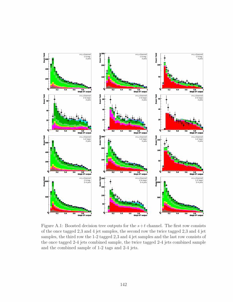
tbtqb DT output0 0.2 0.4 0.6 0.8 1
Eve
nt Y
ield
0
200
400
600
-channelµe+1 b-tag
2 jets
tbtqb DT output0 0.2 0.4 0.6 0.8 1
Eve
nt Y
ield
0
200
400
600
tbtqb DT output0 0.2 0.4 0.6 0.8 1
Eve
nt Y
ield
0
100
200
300 -channelµe+1 b-tag
3 jets
tbtqb DT output0 0.2 0.4 0.6 0.8 1
Eve
nt Y
ield
0
100
200
300
tbtqb DT output0 0.2 0.4 0.6 0.8 1
Eve
nt Y
ield
0
50
100
-channelµe+1 b-tag
4 jets
tbtqb DT output0 0.2 0.4 0.6 0.8 1
Eve
nt Y
ield
0
50
100
tbtqb DT output0 0.2 0.4 0.6 0.8 1
Eve
nt Y
ield
0
20
40
60
-channelµe+2 b-tags
2 jets
tbtqb DT output0 0.2 0.4 0.6 0.8 1
Eve
nt Y
ield
0
20
40
60
tbtqb DT output0 0.2 0.4 0.6 0.8 1
Eve
nt Y
ield
0
20
40
60
-channelµe+2 b-tags
3 jets
tbtqb DT output0 0.2 0.4 0.6 0.8 1
Eve
nt Y
ield
0
20
40
60
tbtqb DT output0 0.2 0.4 0.6 0.8 1
Eve
nt Y
ield
0
20
40
60
-channelµe+2 b-tags
4 jets
tbtqb DT output0 0.2 0.4 0.6 0.8 1
Eve
nt Y
ield
0
20
40
60
tbtqb DT output0 0.2 0.4 0.6 0.8 1
Eve
nt Y
ield
0
200
400
600
-channelµe+1-2 tags
2 jets
tbtqb DT output0 0.2 0.4 0.6 0.8 1
Eve
nt Y
ield
0
200
400
600
tbtqb DT output0 0.2 0.4 0.6 0.8 1
Eve
nt Y
ield
0
100
200
300 -channelµe+1-2 tags
3 jets
tbtqb DT output0 0.2 0.4 0.6 0.8 1
Eve
nt Y
ield
0
100
200
300
tbtqb DT output0 0.2 0.4 0.6 0.8 1
Eve
nt Y
ield
0
50
100
150
-channelµe+1-2 tags
4 jets
tbtqb DT output0 0.2 0.4 0.6 0.8 1
Eve
nt Y
ield
0
50
100
150
tbtqb DT output0 0.2 0.4 0.6 0.8 1
Eve
nt Y
ield
0
500
1000
-channelµe+1 b-tag 2-4 jets
tbtqb DT output0 0.2 0.4 0.6 0.8 1
Eve
nt Y
ield
0
500
1000
tbtqb DT output0 0.2 0.4 0.6 0.8 1
Eve
nt Y
ield
0
50
100
150
200 -channelµe+2 b-tags2-4 jets
tbtqb DT output0 0.2 0.4 0.6 0.8 1
Eve
nt Y
ield
0
50
100
150
200
tbtqb DT output0 0.2 0.4 0.6 0.8 1
Eve
nt Y
ield
0
500
1000
-channelµe+1-2 tags2-4 jets
tbtqb DT output0 0.2 0.4 0.6 0.8 1
Eve
nt Y
ield
0
500
1000
Figure A.1: Boosted decision tree outputs for the s+ t channel. The first row consistsof the once tagged 2,3 and 4 jet samples, the second row the twice tagged 2,3 and 4 jetsamples, the third row the 1-2 tagged 2,3 and 4 jet samples and the last row consists ofthe once tagged 2-4 jets combined sample, the twice tagged 2-4 jets combined sampleand the combined sample of 1-2 tags and 2-4 jets.
142
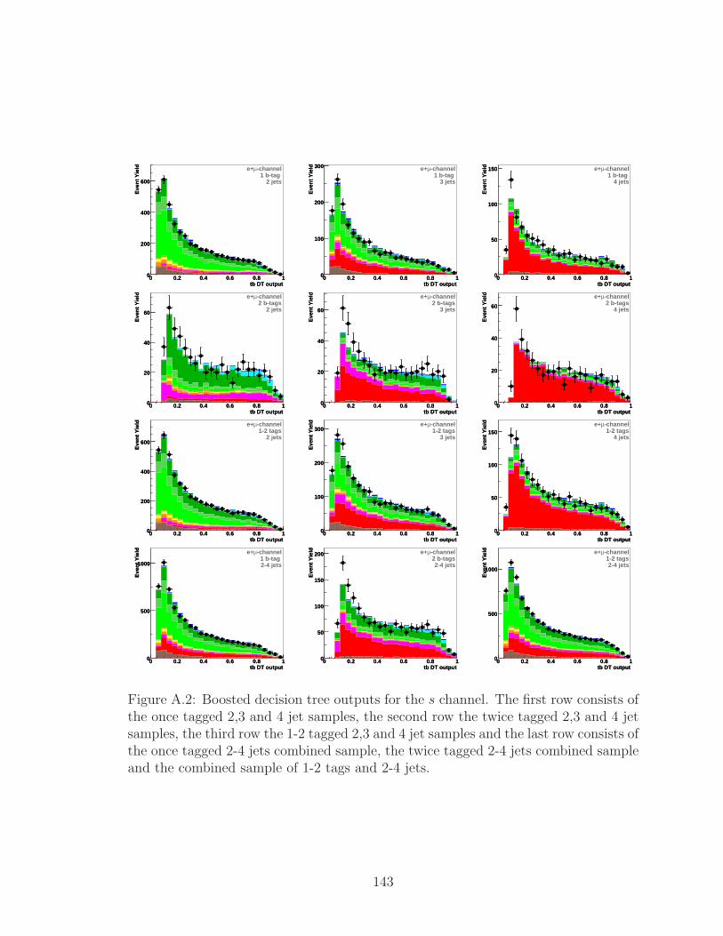
tb DT output0 0.2 0.4 0.6 0.8 1
Eve
nt Y
ield
0
200
400
600
-channelµe+1 b-tag
2 jets
tb DT output0 0.2 0.4 0.6 0.8 1
Eve
nt Y
ield
0
200
400
600
tb DT output0 0.2 0.4 0.6 0.8 1
Eve
nt Y
ield
0
100
200
300 -channelµe+1 b-tag
3 jets
tb DT output0 0.2 0.4 0.6 0.8 1
Eve
nt Y
ield
0
100
200
300
tb DT output0 0.2 0.4 0.6 0.8 1
Eve
nt Y
ield
0
50
100
150 -channelµe+1 b-tag
4 jets
tb DT output0 0.2 0.4 0.6 0.8 1
Eve
nt Y
ield
0
50
100
150
tb DT output0 0.2 0.4 0.6 0.8 1
Eve
nt Y
ield
0
20
40
60
-channelµe+2 b-tags
2 jets
tb DT output0 0.2 0.4 0.6 0.8 1
Eve
nt Y
ield
0
20
40
60
tb DT output0 0.2 0.4 0.6 0.8 1
Eve
nt Y
ield
0
20
40
60
-channelµe+2 b-tags
3 jets
tb DT output0 0.2 0.4 0.6 0.8 1
Eve
nt Y
ield
0
20
40
60
tb DT output0 0.2 0.4 0.6 0.8 1
Eve
nt Y
ield
0
20
40
60
-channelµe+2 b-tags
4 jets
tb DT output0 0.2 0.4 0.6 0.8 1
Eve
nt Y
ield
0
20
40
60
tb DT output0 0.2 0.4 0.6 0.8 1
Eve
nt Y
ield
0
200
400
600
-channelµe+1-2 tags
2 jets
tb DT output0 0.2 0.4 0.6 0.8 1
Eve
nt Y
ield
0
200
400
600
tb DT output0 0.2 0.4 0.6 0.8 1
Eve
nt Y
ield
0
100
200
300-channelµe+1-2 tags
3 jets
tb DT output0 0.2 0.4 0.6 0.8 1
Eve
nt Y
ield
0
100
200
300
tb DT output0 0.2 0.4 0.6 0.8 1
Eve
nt Y
ield
0
50
100
150-channelµe+1-2 tags
4 jets
tb DT output0 0.2 0.4 0.6 0.8 1
Eve
nt Y
ield
0
50
100
150
tb DT output0 0.2 0.4 0.6 0.8 1
Eve
nt Y
ield
0
500
1000
-channelµe+1 b-tag 2-4 jets
tb DT output0 0.2 0.4 0.6 0.8 1
Eve
nt Y
ield
0
500
1000
tb DT output0 0.2 0.4 0.6 0.8 1
Eve
nt Y
ield
0
50
100
150
200 -channelµe+2 b-tags2-4 jets
tb DT output0 0.2 0.4 0.6 0.8 1
Eve
nt Y
ield
0
50
100
150
200
tb DT output0 0.2 0.4 0.6 0.8 1
Eve
nt Y
ield
0
500
1000
-channelµe+1-2 tags2-4 jets
tb DT output0 0.2 0.4 0.6 0.8 1
Eve
nt Y
ield
0
500
1000
Figure A.2: Boosted decision tree outputs for the s channel. The first row consists ofthe once tagged 2,3 and 4 jet samples, the second row the twice tagged 2,3 and 4 jetsamples, the third row the 1-2 tagged 2,3 and 4 jet samples and the last row consists ofthe once tagged 2-4 jets combined sample, the twice tagged 2-4 jets combined sampleand the combined sample of 1-2 tags and 2-4 jets.
143
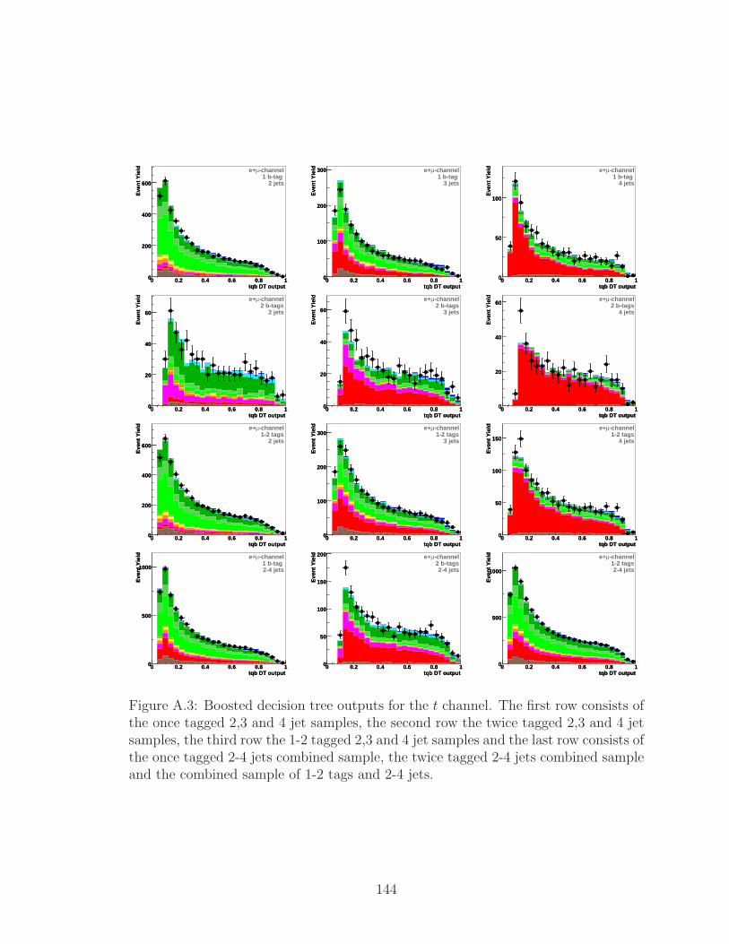
tqb DT output0 0.2 0.4 0.6 0.8 1
Eve
nt Y
ield
0
200
400
600
-channelµe+1 b-tag
2 jets
tqb DT output0 0.2 0.4 0.6 0.8 1
Eve
nt Y
ield
0
200
400
600
tqb DT output0 0.2 0.4 0.6 0.8 1
Eve
nt Y
ield
0
100
200
300 -channelµe+1 b-tag
3 jets
tqb DT output0 0.2 0.4 0.6 0.8 1
Eve
nt Y
ield
0
100
200
300
tqb DT output0 0.2 0.4 0.6 0.8 1
Eve
nt Y
ield
0
50
100
-channelµe+1 b-tag
4 jets
tqb DT output0 0.2 0.4 0.6 0.8 1
Eve
nt Y
ield
0
50
100
tqb DT output0 0.2 0.4 0.6 0.8 1
Eve
nt Y
ield
0
20
40
60
-channelµe+2 b-tags
2 jets
tqb DT output0 0.2 0.4 0.6 0.8 1
Eve
nt Y
ield
0
20
40
60
tqb DT output0 0.2 0.4 0.6 0.8 1
Eve
nt Y
ield
0
20
40
60
-channelµe+2 b-tags
3 jets
tqb DT output0 0.2 0.4 0.6 0.8 1
Eve
nt Y
ield
0
20
40
60
tqb DT output0 0.2 0.4 0.6 0.8 1
Eve
nt Y
ield
0
20
40
60-channelµe+2 b-tags
4 jets
tqb DT output0 0.2 0.4 0.6 0.8 1
Eve
nt Y
ield
0
20
40
60
tqb DT output0 0.2 0.4 0.6 0.8 1
Eve
nt Y
ield
0
200
400
600
-channelµe+1-2 tags
2 jets
tqb DT output0 0.2 0.4 0.6 0.8 1
Eve
nt Y
ield
0
200
400
600
tqb DT output0 0.2 0.4 0.6 0.8 1
Eve
nt Y
ield
0
100
200
300-channelµe+1-2 tags
3 jets
tqb DT output0 0.2 0.4 0.6 0.8 1
Eve
nt Y
ield
0
100
200
300
tqb DT output0 0.2 0.4 0.6 0.8 1
Eve
nt Y
ield
0
50
100
150
-channelµe+1-2 tags
4 jets
tqb DT output0 0.2 0.4 0.6 0.8 1
Eve
nt Y
ield
0
50
100
150
tqb DT output0 0.2 0.4 0.6 0.8 1
Eve
nt Y
ield
0
500
1000
-channelµe+1 b-tag 2-4 jets
tqb DT output0 0.2 0.4 0.6 0.8 1
Eve
nt Y
ield
0
500
1000
tqb DT output0 0.2 0.4 0.6 0.8 1
Eve
nt Y
ield
0
50
100
150
200 -channelµe+2 b-tags2-4 jets
tqb DT output0 0.2 0.4 0.6 0.8 1
Eve
nt Y
ield
0
50
100
150
200
tqb DT output0 0.2 0.4 0.6 0.8 1
Eve
nt Y
ield
0
500
1000
-channelµe+1-2 tags2-4 jets
tqb DT output0 0.2 0.4 0.6 0.8 1
Eve
nt Y
ield
0
500
1000
Figure A.3: Boosted decision tree outputs for the t channel. The first row consists ofthe once tagged 2,3 and 4 jet samples, the second row the twice tagged 2,3 and 4 jetsamples, the third row the 1-2 tagged 2,3 and 4 jet samples and the last row consists ofthe once tagged 2-4 jets combined sample, the twice tagged 2-4 jets combined sampleand the combined sample of 1-2 tags and 2-4 jets.
144
Appendix B
Residual Systematic Errors
B.1 Normalization Uncertainties
Tables B.1- B.6 show the effects of the systematic uncertainties (Section 6.3.1) for
the six jet and b tag categories used in the analysis. The values listed here are used
as inputs to the BDT discriminants that are used to measure the single top cross
sections. It should be noted that systematic samples which have a minus sign are
considered anti-correlated with other samples in the same row. This is a constraint
implemented in this analysis to preserve normalization.
145

UNCERTAINTIES FOR CHANNELS WITH TWO JETS
SINGLE TAG
Uncertainties %
Source ttll ttlj Wbb Wcc Wlp Zbb Zcc Zlp dibosons QCD tb t tb + t
Luminosity 6.1 6.1 — — — 6.1 6.1 6.1 6.1 — 6.1 6.1 6.1Cross section 9.0 9.0 — — — 3.3 3.3 3.3 7.0 — 3.8 5.3 4.8Branching fraction 1.5 1.5 — — — — — — — — 1.5 1.5 1.5PDF — — — — — — — — — — 2.0 2.0 2.0Triggers 5.0 5.0 — — — 5.0 5.0 5.0 5.0 — 5.0 5.0 5.0Luminosity 1.0 1.0 — — — 1.0 1.0 1.0 1.0 — 1.0 1.0 1.0ReweightingPrimary Vertex 1.4 1.4 — — — 1.4 1.4 1.4 1.4 — 1.4 1.4 1.4ReweightingColor Reconnection 1.0 1.0 — — — — — — — — 1.0 1.0 1.0b/light Jet Response −0.4 −0.4 — — — 1.0 — — — — 0.5 0.5 0.5Lepton ID 2.9 2.9 — — — 2.4 2.4 2.6 2.7 — 2.8 2.8 2.8Jet fragmentation and 1.6 1.6 — — — — — — — — 0.7 0.7 0.7higher orderISR/FSR 4.3 4.3 — — — — — — — — 0.8 0.8 0.8b-jet fragmentation 2.0 2.0 — — — 2.0 — — — — 2.0 2.0 2.0Taggability 7.1 5.6 5.6 5.1 6.2 6.2 6.4 5.8 5.7 — 6.6 5.9 6.1
λW
HF— — 12.0 12.0 — — — — — — — — —
λZ
HF— — — — — 12.0 12.0 — — — — — —
W+Jet and QCD — — 1.8 1.8 1.8 — — — — −34.6 — — —
Table B.1: Residual normalization systematic uncertainties: two jets with 1-btag.These values are used as input parameters to the BDT analysis.
DOUBLE TAG
Uncertainties %
Source ttll ttlj Wbb Wcc Wlp Zbb Zcc Zlp dibosons QCD tb t tb + t
Luminosity 6.1 6.1 — — — 6.1 6.1 6.1 6.1 — 6.1 6.1 6.1Cros section 9.0 9.0 — — — 3.3 3.3 3.3 7.0 — 3.8 5.3 4.8Branching fraction 1.5 1.5 — — — — — — — — 1.5 1.5 1.5PDF — — — — — — — — — — 2.0 2.0 2.0Triggers 5.0 5.0 — — — 5.0 5.0 5.0 5.0 — 5.0 5.0 5.0Luminosity 1.0 1.0 — — — 1.0 1.0 1.0 1.0 — 1.0 1.0 1.0ReweightingPrimary Vertex 1.4 1.4 — — — 1.4 1.4 1.4 1.4 — 1.4 1.4 1.4ReweightingColor Reconnection 1.0 1.0 — — — — — — — — 1.0 1.0 1.0b/light Jet Response −0.4 −0.4 — — — 1.0 — — — — 0.5 0.5 0.5Lepton ID 2.9 2.8 — — — 2.3 2.4 3.2 2.7 — 2.8 2.8 2.8Jet fragmentation and 1.6 1.6 — — — — — — — — 0.7 0.7 0.7higher orderISR/FSR 4.3 4.3 — — — — — — — — 0.8 0.8 0.8b-jet fragmentation 2.0 2.0 — — — 2.0 — — — — 2.0 2.0 2.0Taggability 3.5 3.2 3.8 3.7 4.4 3.8 3.4 3.6 3.4 — 3.5 3.9 3.6
λW
HF— — 12.0 12.0 — — — — — — — — —
λZ
HF— — — — — 12.0 12.0 — — — — — —
W+Jet and QCD — — 1.8 1.8 1.8 — — — — −34.9 — — —
Table B.2: Residual normalization systematic uncertainties: two jets with 2-btags.These values are used as input parameters to the BDT analysis.
146

UNCERTAINTIES FOR CHANNELS WITH THREE JETS
SINGLE TAG
Uncertainties %
Source ttll ttlj Wbb Wcc Wlp Zbb Zcc Zlp dibosons QCD tb t tb + t
Luminosity 6.1 6.1 — — — 6.1 6.1 6.1 6.1 — 6.1 6.1 6.1Cross section 9.0 9.0 — — — 3.3 3.3 3.3 7.0 — 3.8 5.3 4.8Branching fraction 1.5 1.5 — — — — — — — — 1.5 1.5 1.5PDF — — — — — — — — — — 2.0 2.0 2.0Triggers 5.0 5.0 — — — 5.0 5.0 5.0 5.0 — 5.0 5.0 5.0Luminosity 1.0 1.0 — — — 1.0 1.0 1.0 1.0 — 1.0 1.0 1.0ReweightingPrimary Vertex 1.4 1.4 — — — 1.4 1.4 1.4 1.4 — 1.4 1.4 1.4ReweightingColor Reconnection 1.0 1.0 — — — — — — — — 1.0 1.0 1.0b/light Jet Response 0.0 0.0 — — — 0.6 — — — — 0.8 0.8 0.8Lepton ID 2.8 2.8 — — — 2.5 2.5 2.7 2.7 — 2.7 2.8 2.8Jet fragmentation and 1.7 1.7 — — — — — — — — 3.7 3.7 3.7higher orderISR/FSR 2.2 2.2 — — — — — — — — −5.9 −5.9 −5.9b-jet fragmentation 2.0 2.0 — — — 2.0 — — — — 2.0 2.0 2.0Taggability 13.3 8.6 7.9 8.0 8.8 9.4 7.7 14.8 8.7 — 9.3 8.6 8.9
λW
HF— — 12.0 12.0 — — — — — — — — —
λZ
HF— — — — — 12.0 12.0 — — — — — —
W+Jet and QCD — — 1.8 1.8 1.8 — — — — −36.2 — — —
Table B.3: Residual normalization systematic uncertainties: three jets with 1-btag.These values are used as input parameters to the BDT analysis.
DOUBLE TAG
Uncertainties %
Source ttll ttlj Wbb Wcc Wlp Zbb Zcc Zlp dibosons QCD tb t tb + t
Luminosity 6.1 6.1 — — — 6.1 6.1 6.1 6.1 — 6.1 6.1 6.1Cross section 9.0 9.0 — — — 3.3 3.3 3.3 7.0 — 3.8 5.3 4.8Branching fraction 1.5 1.5 — — — — — — — — 1.5 1.5 1.5PDF — — — — — — — — — — 2.0 2.0 2.0Triggers 5.0 5.0 — — — 5.0 5.0 5.0 5.0 — 5.0 5.0 5.0Luminosity 1.0 1.0 — — — 1.0 1.0 1.0 1.0 — 1.0 1.0 1.0ReweightingPrimary Vertex 1.4 1.4 — — — 1.4 1.4 1.4 1.4 — 1.4 1.4 1.4ReweightingColor Reconnection 1.0 1.0 — — — — — — — — 1.0 1.0 1.0b/light Jet Response 0.0 0.0 — — — 0.6 — — — — 0.8 0.8 0.8Lepton ID 2.8 2.8 — — — 2.5 2.4 2.2 2.7 — 2.8 2.8 2.8Jet fragmentation and 1.7 1.7 — — — — — — — — 3.7 3.7 3.7higher orderISR/FSR 2.2 2.2 — — — — — — — — −5.9 −5.9 −5.9b-jet fragmentation 2.0 2.0 — — — 2.0 — — — — 2.0 2.0 2.0Taggability 9.3 5.9 6.8 6.6 6.7 6.9 7.2 6.3 8.4 — 6.3 6.4 6.4
λW
HF— — 12.0 12.0 — — — — — — — — —
λZ
HF— — — — — 12.0 12.0 — — — — — —
W+Jet and QCD — — 1.8 1.8 1.8 — — — — −36.0 — — —
Table B.4: Residual normalization systematic uncertainties: three jets with 2-btags.These values are used as input parameters to the BDT analysis.
147

UNCERTAINTIES FOR CHANNELS WITH FOUR JETS
SINGLE TAG
Uncertainties %
Source ttll ttlj Wbb Wcc Wlp Zbb Zcc Zlp dibosons QCD tb t tb + t
Luminosity 6.1 6.1 — — — 6.1 6.1 6.1 6.1 — 6.1 6.1 6.1Cross section 9.0 9.0 — — — 3.3 3.3 3.3 7.0 — 3.8 5.3 4.8Branching fraction 1.5 1.5 — — — — — — — — 1.5 1.5 1.5PDF — — — — — — — — — — 2.0 2.0 2.0Triggers 5.0 5.0 — — — 5.0 5.0 5.0 5.0 — 5.0 5.0 5.0Luminosity 1.0 1.0 — — — 1.0 1.0 1.0 1.0 — 1.0 1.0 1.0ReweightingPrimary Vertex 1.4 1.4 — — — 1.4 1.4 1.4 1.4 — 1.4 1.4 1.4ReweightingColor Reconnection 1.0 1.0 — — — — — — — — 1.0 1.0 1.0b/light Jet Response 0.3 0.3 — — — 0.8 — — — — 0.9 0.9 0.9Lepton ID 2.8 2.8 — — — 2.6 2.5 2.4 2.7 — 2.7 2.8 2.8Jet fragmentation and −7.0 −7.0 — — — — — — — — 4.7 4.7 4.7higher orderISR/FSR 0.8 0.8 — — — — — — — — −10.9 −10.9 −10.9b-jet fragmentation 2.0 2.0 — — — 2.0 — — — — 2.0 2.0 2.0Taggability 15.9 11.8 14.9 9.2 14.4 10.6 13.4 10.7 9.5 — 12.6 12.1 12.2
λW
HF— — 12.0 12.0 — — — — — — — — —
λZ
HF— — — — — 12.0 12.0 — — — — — —
W+Jet and QCD — — 1.8 1.8 1.8 — — — — −33.8 — — —
Table B.5: Residual normalization systematic uncertainties: four jets with 1-btag.These values are used as input parameters to the BDT analysis.
DOUBLE TAG
Uncertainties %
Source ttll ttlj Wbb Wcc Wlp Zbb Zcc Zlp dibosons QCD tb t tb + t
Luminosity 6.1 6.1 — — — 6.1 6.1 6.1 6.1 — 6.1 6.1 6.1Cross section 9.0 9.0 — — — 3.3 3.3 3.3 7.0 — 3.8 5.3 4.8Branching fraction 1.5 1.5 — — — — — — — — 1.5 1.5 1.5PDF — — — — — — — — — — 2.0 2.0 2.0Triggers 5.0 5.0 — — — 5.0 5.0 5.0 5.0 — 5.0 5.0 5.0Luminosity 1.0 1.0 — — — 1.0 1.0 1.0 1.0 — 1.0 1.0 1.0ReweightingPrimary Vertex 1.4 1.4 — — — 1.4 1.4 1.4 1.4 — 1.4 1.4 1.4ReweightingColor Reconnection 1.0 1.0 — — — — — — — — 1.0 1.0 1.0b/light Jet Response 0.3 0.3 — — — 0.8 — — — — 0.9 0.9 0.9Lepton ID 2.8 2.8 — — — 2.6 2.6 2.4 2.7 — 2.8 2.8 2.8Jet fragmentation and −7.0 −7.0 — — — — — — — — 4.7 4.7 4.7higher orderISR/FSR 0.8 0.8 — — — — — — — — −10.9 −10.9 −10.9b-jet fragmetation 2.0 2.0 — — — 2.0 — — — — 2.0 2.0 2.0Taggability 11.7 8.2 9.8 6.4 8.8 9.7 18.4 21.1 7.7 — 8.6 14.1 11.7
λW
HF— — 12.0 12.0 — — — — — — — — —
λZ
HF— — — — — 12.0 12.0 — — — — — —
W+Jet and QCD — — 1.8 1.8 1.8 — — — — −34.3 — — —
Table B.6: Residual normalization systematic uncertainties: four jets with 2-btags.These values are used as input parameters to the BDT analysis.
148

B.2 Shape and Normalization Uncertainties
The systematic uncertainties that change both the normalization and the shape of the
kinematic distributions are: jet reconstruction and identification,(JetID), jet energy
scale (JES), jet energy resolution (JER), primary vertex confirmation (VC), V+jets
angular corrections (AC), b tag scale factors (BTag). These systematics are divided
into two groups. The first being corrections that are applied before event selection
and the other after event selection. The JetID, JES, JER, and VC corrections are
all applied before event selection and change the amount of events passing selection,
event weight and jet multiplicity. The AC and BTag corrections are applied after
selection and only change event weight.
Figures [B.1-B.4] show the effects of each of these uncertainties on the boosted de-
cision tree output discriminants for s+t, s and t channel analyses. The AC systematic
is not included because the change in shape is very small.
149

0.1 0.2 0.3 0.4 0.5 0.6 0.7 0.8 0.90.4
0.6
0.8
1
1.2
1.4
1.6
1.8
JETIDσ +1
nominalJETIDσ -1
DT_output {EventWeight*(1)}
0.2 0.3 0.4 0.5 0.6 0.7 0.80.4
0.6
0.8
1
1.2
1.4
1.6
1.8
JETIDσ +1
nominalJETIDσ -1
DT_output {EventWeight*(1)}
0.1 0.2 0.3 0.4 0.5 0.6 0.7 0.80.4
0.6
0.8
1
1.2
1.4
1.6
1.8
JETIDσ +1
nominalJETIDσ -1
DT_output {EventWeight*(1)}
0.1 0.2 0.3 0.4 0.5 0.6 0.7 0.8 0.90.4
0.6
0.8
1
1.2
1.4
1.6
1.8
JESσ +1
nominalJESσ -1
DT_output {EventWeight*(1)}
0.2 0.3 0.4 0.5 0.6 0.7 0.80.4
0.6
0.8
1
1.2
1.4
1.6
1.8
JESσ +1
nominalJESσ -1
DT_output {EventWeight*(1)}
0.1 0.2 0.3 0.4 0.5 0.6 0.7 0.80.4
0.6
0.8
1
1.2
1.4
1.6
1.8
JESσ +1
nominalJESσ -1
DT_output {EventWeight*(1)}
0.1 0.2 0.3 0.4 0.5 0.6 0.7 0.8 0.90.4
0.6
0.8
1
1.2
1.4
1.6
1.8
JERσ +1
nominalJERσ -1
DT_output {EventWeight*(1)}
0.2 0.3 0.4 0.5 0.6 0.7 0.80.4
0.6
0.8
1
1.2
1.4
1.6
1.8
JERσ +1
nominalJERσ -1
DT_output {EventWeight*(1)}
0.1 0.2 0.3 0.4 0.5 0.6 0.7 0.80.4
0.6
0.8
1
1.2
1.4
1.6
1.8
JERσ +1
nominalJERσ -1
DT_output {EventWeight*(1)}
0.1 0.2 0.3 0.4 0.5 0.6 0.7 0.8 0.90.4
0.6
0.8
1
1.2
1.4
1.6
1.8
VCσ +1
nominalVCσ -1
DT_output {EventWeight*(1)}
0.2 0.3 0.4 0.5 0.6 0.7 0.80.4
0.6
0.8
1
1.2
1.4
1.6
1.8
VCσ +1
nominalVCσ -1
DT_output {EventWeight*(1)}
0.1 0.2 0.3 0.4 0.5 0.6 0.7 0.80.4
0.6
0.8
1
1.2
1.4
1.6
1.8
VCσ +1
nominalVCσ -1
DT_output {EventWeight*(1)}
0.1 0.2 0.3 0.4 0.5 0.6 0.7 0.8 0.90.4
0.6
0.8
1
1.2
1.4
1.6
1.8
BTagσ +1
nominalBTagσ -1
DT_output {EventWeight*(1)}
0.2 0.3 0.4 0.5 0.6 0.7 0.80.4
0.6
0.8
1
1.2
1.4
1.6
1.8
BTagσ +1
nominalBTagσ -1
DT_output {EventWeight*(1)}
0.1 0.2 0.3 0.4 0.5 0.6 0.7 0.80.4
0.6
0.8
1
1.2
1.4
1.6
1.8
BTagσ +1
nominalBTagσ -1
DT_output {EventWeight*(1)}
Figure B.1: Combined s+ t channel discriminant, showing the effects of a ±1 fluctua-tion in each systematic. The plots are for events with a single b tag. The left columnis for the 2 jet events, the center column is for 3 jet events and the right column isfor 4 jet events.
150
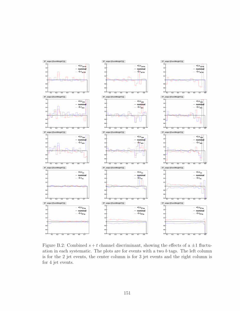
0.1 0.2 0.3 0.4 0.5 0.6 0.70.4
0.6
0.8
1
1.2
1.4
1.6
1.8
JETIDσ +1
nominalJETIDσ -1
DT_output {EventWeight*(1)}
0.2 0.3 0.4 0.5 0.6 0.7 0.80.4
0.6
0.8
1
1.2
1.4
1.6
1.8
JETIDσ +1
nominalJETIDσ -1
DT_output {EventWeight*(1)}
0.1 0.2 0.3 0.4 0.5 0.6 0.7 0.80.4
0.6
0.8
1
1.2
1.4
1.6
1.8
JETIDσ +1
nominalJETIDσ -1
DT_output {EventWeight*(1)}
0.1 0.2 0.3 0.4 0.5 0.6 0.70.4
0.6
0.8
1
1.2
1.4
1.6
1.8
JESσ +1
nominalJESσ -1
DT_output {EventWeight*(1)}
0.2 0.3 0.4 0.5 0.6 0.7 0.80.4
0.6
0.8
1
1.2
1.4
1.6
1.8
JESσ +1
nominalJESσ -1
DT_output {EventWeight*(1)}
0.1 0.2 0.3 0.4 0.5 0.6 0.7 0.80.4
0.6
0.8
1
1.2
1.4
1.6
1.8
JESσ +1
nominalJESσ -1
DT_output {EventWeight*(1)}
0.1 0.2 0.3 0.4 0.5 0.6 0.70.4
0.6
0.8
1
1.2
1.4
1.6
1.8
JERσ +1
nominalJERσ -1
DT_output {EventWeight*(1)}
0.2 0.3 0.4 0.5 0.6 0.7 0.80.4
0.6
0.8
1
1.2
1.4
1.6
1.8
JERσ +1
nominalJERσ -1
DT_output {EventWeight*(1)}
0.1 0.2 0.3 0.4 0.5 0.6 0.7 0.80.4
0.6
0.8
1
1.2
1.4
1.6
1.8
JERσ +1
nominalJERσ -1
DT_output {EventWeight*(1)}
0.1 0.2 0.3 0.4 0.5 0.6 0.70.4
0.6
0.8
1
1.2
1.4
1.6
1.8
VCσ +1
nominalVCσ -1
DT_output {EventWeight*(1)}
0.2 0.3 0.4 0.5 0.6 0.7 0.80.4
0.6
0.8
1
1.2
1.4
1.6
1.8
VCσ +1
nominalVCσ -1
DT_output {EventWeight*(1)}
0.1 0.2 0.3 0.4 0.5 0.6 0.7 0.80.4
0.6
0.8
1
1.2
1.4
1.6
1.8
VCσ +1
nominalVCσ -1
DT_output {EventWeight*(1)}
0.1 0.2 0.3 0.4 0.5 0.6 0.70.4
0.6
0.8
1
1.2
1.4
1.6
1.8
BTagσ +1
nominalBTagσ -1
DT_output {EventWeight*(1)}
0.2 0.3 0.4 0.5 0.6 0.7 0.80.4
0.6
0.8
1
1.2
1.4
1.6
1.8
BTagσ +1
nominalBTagσ -1
DT_output {EventWeight*(1)}
0.1 0.2 0.3 0.4 0.5 0.6 0.7 0.80.4
0.6
0.8
1
1.2
1.4
1.6
1.8
BTagσ +1
nominalBTagσ -1
DT_output {EventWeight*(1)}
Figure B.2: Combined s+ t channel discriminant, showing the effects of a ±1 fluctu-ation in each systematic. The plots are for events with a two b tags. The left columnis for the 2 jet events, the center column is for 3 jet events and the right column isfor 4 jet events.
151

0.1 0.2 0.3 0.4 0.5 0.6 0.7 0.80.4
0.6
0.8
1
1.2
1.4
1.6
1.8
JETIDσ +1
nominalJETIDσ -1
DT_tb_output {EventWeight*(1)}
0.1 0.2 0.3 0.4 0.5 0.6 0.70.4
0.6
0.8
1
1.2
1.4
1.6
1.8
JETIDσ +1
nominalJETIDσ -1
DT_tb_output {EventWeight*(1)}
0.1 0.2 0.3 0.4 0.5 0.6 0.70.4
0.6
0.8
1
1.2
1.4
1.6
1.8
JETIDσ +1
nominalJETIDσ -1
DT_tb_output {EventWeight*(1)}
0.1 0.2 0.3 0.4 0.5 0.6 0.7 0.80.4
0.6
0.8
1
1.2
1.4
1.6
1.8
JESσ +1
nominalJESσ -1
DT_tb_output {EventWeight*(1)}
0.1 0.2 0.3 0.4 0.5 0.6 0.70.4
0.6
0.8
1
1.2
1.4
1.6
1.8
JESσ +1
nominalJESσ -1
DT_tb_output {EventWeight*(1)}
0.1 0.2 0.3 0.4 0.5 0.6 0.70.4
0.6
0.8
1
1.2
1.4
1.6
1.8
JESσ +1
nominalJESσ -1
DT_tb_output {EventWeight*(1)}
0.1 0.2 0.3 0.4 0.5 0.6 0.7 0.80.4
0.6
0.8
1
1.2
1.4
1.6
1.8
JERσ +1
nominalJERσ -1
DT_tb_output {EventWeight*(1)}
0.1 0.2 0.3 0.4 0.5 0.6 0.70.4
0.6
0.8
1
1.2
1.4
1.6
1.8
JERσ +1
nominalJERσ -1
DT_tb_output {EventWeight*(1)}
0.1 0.2 0.3 0.4 0.5 0.6 0.70.4
0.6
0.8
1
1.2
1.4
1.6
1.8
JERσ +1
nominalJERσ -1
DT_tb_output {EventWeight*(1)}
0.1 0.2 0.3 0.4 0.5 0.6 0.7 0.80.4
0.6
0.8
1
1.2
1.4
1.6
1.8
VCσ +1
nominalVCσ -1
DT_tb_output {EventWeight*(1)}
0.1 0.2 0.3 0.4 0.5 0.6 0.70.4
0.6
0.8
1
1.2
1.4
1.6
1.8
VCσ +1
nominalVCσ -1
DT_tb_output {EventWeight*(1)}
0.1 0.2 0.3 0.4 0.5 0.6 0.70.4
0.6
0.8
1
1.2
1.4
1.6
1.8
VCσ +1
nominalVCσ -1
DT_tb_output {EventWeight*(1)}
0.1 0.2 0.3 0.4 0.5 0.6 0.7 0.80.4
0.6
0.8
1
1.2
1.4
1.6
1.8
BTagσ +1
nominalBTagσ -1
DT_tb_output {EventWeight*(1)}
0.1 0.2 0.3 0.4 0.5 0.6 0.70.4
0.6
0.8
1
1.2
1.4
1.6
1.8
BTagσ +1
nominalBTagσ -1
DT_tb_output {EventWeight*(1)}
0.1 0.2 0.3 0.4 0.5 0.6 0.70.4
0.6
0.8
1
1.2
1.4
1.6
1.8
BTagσ +1
nominalBTagσ -1
DT_tb_output {EventWeight*(1)}
Figure B.3: Combined s channel discriminant, showing the effects of a ±1 fluctuationin each systematic. The plots are for events with a single b tag. The left column isfor the 2 jet events, the center column is for 3 jet events and the right column is for4 jet events.
152
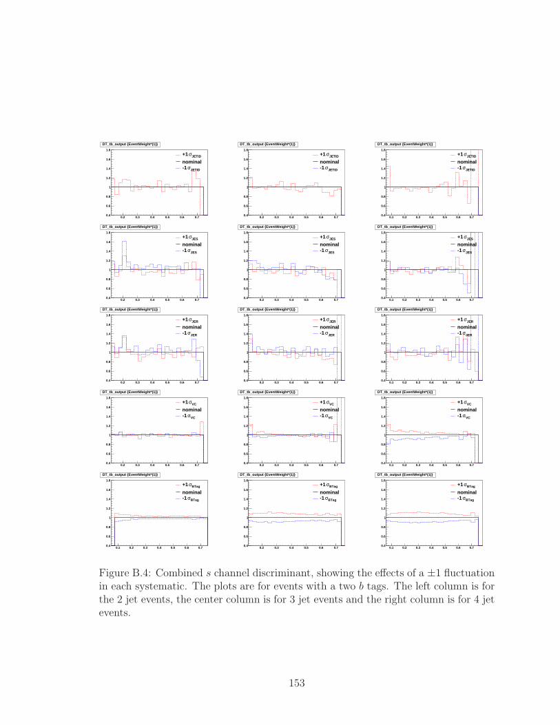
0.2 0.3 0.4 0.5 0.6 0.70.4
0.6
0.8
1
1.2
1.4
1.6
1.8
JETIDσ +1
nominalJETIDσ -1
DT_tb_output {EventWeight*(1)}
0.2 0.3 0.4 0.5 0.6 0.70.4
0.6
0.8
1
1.2
1.4
1.6
1.8
JETIDσ +1
nominalJETIDσ -1
DT_tb_output {EventWeight*(1)}
0.1 0.2 0.3 0.4 0.5 0.6 0.70.4
0.6
0.8
1
1.2
1.4
1.6
1.8
JETIDσ +1
nominalJETIDσ -1
DT_tb_output {EventWeight*(1)}
0.2 0.3 0.4 0.5 0.6 0.70.4
0.6
0.8
1
1.2
1.4
1.6
1.8
JESσ +1
nominalJESσ -1
DT_tb_output {EventWeight*(1)}
0.2 0.3 0.4 0.5 0.6 0.70.4
0.6
0.8
1
1.2
1.4
1.6
1.8
JESσ +1
nominalJESσ -1
DT_tb_output {EventWeight*(1)}
0.1 0.2 0.3 0.4 0.5 0.6 0.70.4
0.6
0.8
1
1.2
1.4
1.6
1.8
JESσ +1
nominalJESσ -1
DT_tb_output {EventWeight*(1)}
0.2 0.3 0.4 0.5 0.6 0.70.4
0.6
0.8
1
1.2
1.4
1.6
1.8
JERσ +1
nominalJERσ -1
DT_tb_output {EventWeight*(1)}
0.2 0.3 0.4 0.5 0.6 0.70.4
0.6
0.8
1
1.2
1.4
1.6
1.8
JERσ +1
nominalJERσ -1
DT_tb_output {EventWeight*(1)}
0.1 0.2 0.3 0.4 0.5 0.6 0.70.4
0.6
0.8
1
1.2
1.4
1.6
1.8
JERσ +1
nominalJERσ -1
DT_tb_output {EventWeight*(1)}
0.2 0.3 0.4 0.5 0.6 0.70.4
0.6
0.8
1
1.2
1.4
1.6
1.8
VCσ +1
nominalVCσ -1
DT_tb_output {EventWeight*(1)}
0.2 0.3 0.4 0.5 0.6 0.70.4
0.6
0.8
1
1.2
1.4
1.6
1.8
VCσ +1
nominalVCσ -1
DT_tb_output {EventWeight*(1)}
0.1 0.2 0.3 0.4 0.5 0.6 0.70.4
0.6
0.8
1
1.2
1.4
1.6
1.8
VCσ +1
nominalVCσ -1
DT_tb_output {EventWeight*(1)}
0.1 0.2 0.3 0.4 0.5 0.6 0.70.4
0.6
0.8
1
1.2
1.4
1.6
1.8
BTagσ +1
nominalBTagσ -1
DT_tb_output {EventWeight*(1)}
0.2 0.3 0.4 0.5 0.6 0.70.4
0.6
0.8
1
1.2
1.4
1.6
1.8
BTagσ +1
nominalBTagσ -1
DT_tb_output {EventWeight*(1)}
0.1 0.2 0.3 0.4 0.5 0.6 0.70.4
0.6
0.8
1
1.2
1.4
1.6
1.8
BTagσ +1
nominalBTagσ -1
DT_tb_output {EventWeight*(1)}
Figure B.4: Combined s channel discriminant, showing the effects of a ±1 fluctuationin each systematic. The plots are for events with a two b tags. The left column is forthe 2 jet events, the center column is for 3 jet events and the right column is for 4 jetevents.
153
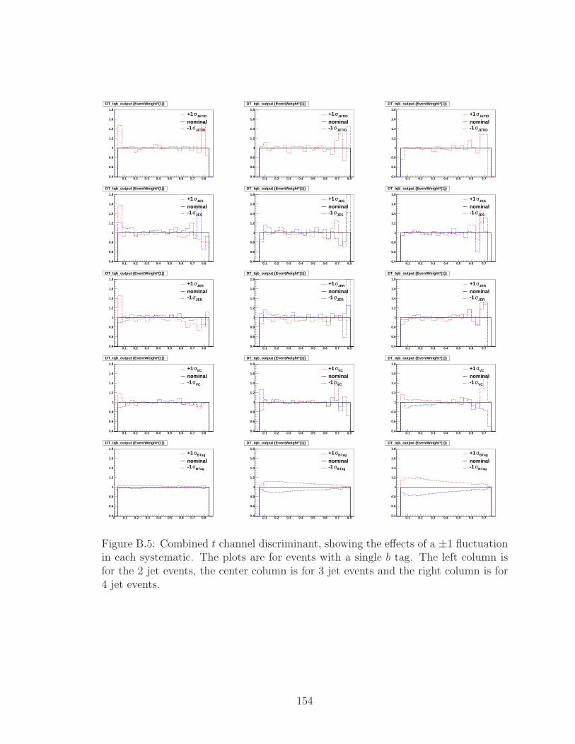
0.1 0.2 0.3 0.4 0.5 0.6 0.7 0.80.4
0.6
0.8
1
1.2
1.4
1.6
1.8
JETIDσ +1
nominalJETIDσ -1
DT_tqb_output {EventWeight*(1)}
0.1 0.2 0.3 0.4 0.5 0.6 0.7 0.80.4
0.6
0.8
1
1.2
1.4
1.6
1.8
JETIDσ +1
nominalJETIDσ -1
DT_tqb_output {EventWeight*(1)}
0.1 0.2 0.3 0.4 0.5 0.6 0.70.4
0.6
0.8
1
1.2
1.4
1.6
1.8
JETIDσ +1
nominalJETIDσ -1
DT_tqb_output {EventWeight*(1)}
0.1 0.2 0.3 0.4 0.5 0.6 0.7 0.80.4
0.6
0.8
1
1.2
1.4
1.6
1.8
JESσ +1
nominalJESσ -1
DT_tqb_output {EventWeight*(1)}
0.1 0.2 0.3 0.4 0.5 0.6 0.7 0.80.4
0.6
0.8
1
1.2
1.4
1.6
1.8
JESσ +1
nominalJESσ -1
DT_tqb_output {EventWeight*(1)}
0.1 0.2 0.3 0.4 0.5 0.6 0.70.4
0.6
0.8
1
1.2
1.4
1.6
1.8
JESσ +1
nominalJESσ -1
DT_tqb_output {EventWeight*(1)}
0.1 0.2 0.3 0.4 0.5 0.6 0.7 0.80.4
0.6
0.8
1
1.2
1.4
1.6
1.8
JERσ +1
nominalJERσ -1
DT_tqb_output {EventWeight*(1)}
0.1 0.2 0.3 0.4 0.5 0.6 0.7 0.80.4
0.6
0.8
1
1.2
1.4
1.6
1.8
JERσ +1
nominalJERσ -1
DT_tqb_output {EventWeight*(1)}
0.1 0.2 0.3 0.4 0.5 0.6 0.70.4
0.6
0.8
1
1.2
1.4
1.6
1.8
JERσ +1
nominalJERσ -1
DT_tqb_output {EventWeight*(1)}
0.1 0.2 0.3 0.4 0.5 0.6 0.7 0.80.4
0.6
0.8
1
1.2
1.4
1.6
1.8
VCσ +1
nominalVCσ -1
DT_tqb_output {EventWeight*(1)}
0.1 0.2 0.3 0.4 0.5 0.6 0.7 0.80.4
0.6
0.8
1
1.2
1.4
1.6
1.8
VCσ +1
nominalVCσ -1
DT_tqb_output {EventWeight*(1)}
0.1 0.2 0.3 0.4 0.5 0.6 0.70.4
0.6
0.8
1
1.2
1.4
1.6
1.8
VCσ +1
nominalVCσ -1
DT_tqb_output {EventWeight*(1)}
0 0.1 0.2 0.3 0.4 0.5 0.6 0.7 0.80.4
0.6
0.8
1
1.2
1.4
1.6
1.8
BTagσ +1
nominalBTagσ -1
DT_tqb_output {EventWeight*(1)}
0.1 0.2 0.3 0.4 0.5 0.6 0.7 0.80.4
0.6
0.8
1
1.2
1.4
1.6
1.8
BTagσ +1
nominalBTagσ -1
DT_tqb_output {EventWeight*(1)}
0.1 0.2 0.3 0.4 0.5 0.6 0.70.4
0.6
0.8
1
1.2
1.4
1.6
1.8
BTagσ +1
nominalBTagσ -1
DT_tqb_output {EventWeight*(1)}
Figure B.5: Combined t channel discriminant, showing the effects of a ±1 fluctuationin each systematic. The plots are for events with a single b tag. The left column isfor the 2 jet events, the center column is for 3 jet events and the right column is for4 jet events.
154
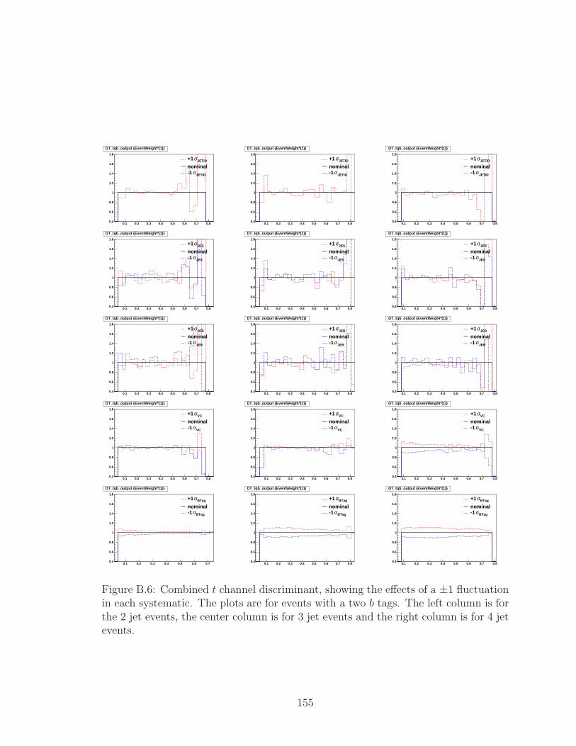
0.1 0.2 0.3 0.4 0.5 0.6 0.7 0.80.4
0.6
0.8
1
1.2
1.4
1.6
1.8
JETIDσ +1
nominalJETIDσ -1
DT_tqb_output {EventWeight*(1)}
0.1 0.2 0.3 0.4 0.5 0.6 0.7 0.80.4
0.6
0.8
1
1.2
1.4
1.6
1.8
JETIDσ +1
nominalJETIDσ -1
DT_tqb_output {EventWeight*(1)}
0.1 0.2 0.3 0.4 0.5 0.6 0.7 0.80.4
0.6
0.8
1
1.2
1.4
1.6
1.8
JETIDσ +1
nominalJETIDσ -1
DT_tqb_output {EventWeight*(1)}
0.1 0.2 0.3 0.4 0.5 0.6 0.7 0.80.4
0.6
0.8
1
1.2
1.4
1.6
1.8
JESσ +1
nominalJESσ -1
DT_tqb_output {EventWeight*(1)}
0.1 0.2 0.3 0.4 0.5 0.6 0.7 0.80.4
0.6
0.8
1
1.2
1.4
1.6
1.8
JESσ +1
nominalJESσ -1
DT_tqb_output {EventWeight*(1)}
0.1 0.2 0.3 0.4 0.5 0.6 0.7 0.80.4
0.6
0.8
1
1.2
1.4
1.6
1.8
JESσ +1
nominalJESσ -1
DT_tqb_output {EventWeight*(1)}
0.1 0.2 0.3 0.4 0.5 0.6 0.7 0.80.4
0.6
0.8
1
1.2
1.4
1.6
1.8
JERσ +1
nominalJERσ -1
DT_tqb_output {EventWeight*(1)}
0.1 0.2 0.3 0.4 0.5 0.6 0.7 0.80.4
0.6
0.8
1
1.2
1.4
1.6
1.8
JERσ +1
nominalJERσ -1
DT_tqb_output {EventWeight*(1)}
0.1 0.2 0.3 0.4 0.5 0.6 0.7 0.80.4
0.6
0.8
1
1.2
1.4
1.6
1.8
JERσ +1
nominalJERσ -1
DT_tqb_output {EventWeight*(1)}
0.1 0.2 0.3 0.4 0.5 0.6 0.7 0.80.4
0.6
0.8
1
1.2
1.4
1.6
1.8
VCσ +1
nominalVCσ -1
DT_tqb_output {EventWeight*(1)}
0.1 0.2 0.3 0.4 0.5 0.6 0.7 0.80.4
0.6
0.8
1
1.2
1.4
1.6
1.8
VCσ +1
nominalVCσ -1
DT_tqb_output {EventWeight*(1)}
0.1 0.2 0.3 0.4 0.5 0.6 0.7 0.80.4
0.6
0.8
1
1.2
1.4
1.6
1.8
VCσ +1
nominalVCσ -1
DT_tqb_output {EventWeight*(1)}
0.1 0.2 0.3 0.4 0.5 0.6 0.70.4
0.6
0.8
1
1.2
1.4
1.6
1.8
BTagσ +1
nominalBTagσ -1
DT_tqb_output {EventWeight*(1)}
0.1 0.2 0.3 0.4 0.5 0.6 0.7 0.80.4
0.6
0.8
1
1.2
1.4
1.6
1.8
BTagσ +1
nominalBTagσ -1
DT_tqb_output {EventWeight*(1)}
0.1 0.2 0.3 0.4 0.5 0.6 0.7 0.80.4
0.6
0.8
1
1.2
1.4
1.6
1.8
BTagσ +1
nominalBTagσ -1
DT_tqb_output {EventWeight*(1)}
Figure B.6: Combined t channel discriminant, showing the effects of a ±1 fluctuationin each systematic. The plots are for events with a two b tags. The left column is forthe 2 jet events, the center column is for 3 jet events and the right column is for 4 jetevents.
155

Bibliography
[1] K. Nakamura et al. (Particle Data Group),“The Review of Particle Physics” J.
Phys. G 37, 075021 (2010).
[2] Wikipedia. Standard model wikipedia, the free encyclopedia, 2011. [Online;
accessed 16-April-2011].
[3] M. Kobayashi, T. Maskawa, “CP-Violation in the Renormalizable Theory of
Weak Interaction”, Progress of Theoretical Physics 49 (2): 652, (1973).
[4] S. W. Herb et al., “Observation of a Dimuon Resonance at 9.5 GeV in 400 GeV
Proton-Nucleus Collisions”, Phys. Rev. Lett. 39,252(1977).
[5] S. Abachi et al.(DØ Collaboration), “Observation of the Top Quark”, Phys. Rev.
Lett. 74, 2632(1995); F. Abe et al.(CDF Collaboration),“Observation of the Top
Quark Production in ppbar Collisions”, Phys. Rev. Lett. 74,2626(1995).
[6] V. Avazov et al.(DØ Collaboration), “Measurement of the top quark pair pro-
duction cross section in the lepton+jets channel in proton-antiproton collisions at
√s=1.96 TeV,” FERMILAB-PUB-10/544-E, Submitted to Phys. Rev. D (2010).
[7] A. Quandt. “Top quark physics at hadron colliders”. The European Journal,
C48:835, (2006).
156

[8] C. Amsler et al., (Particle Data Group), Review of particle physics, Phys. Lett.
B 667, 1 (2008).
[9] A. Heinson, 2011. http://www-d0.fnal.gov/heinson/
[10] V.M. Abazov et al.(DØ Collaboration), “Observation of Single Top Quark Pro-
duction,” Phys. Rev. Lett. 103, 092001 (2009).
[11] N. Kidonakis, “Single Top Quark Production at the Fermilab Tevatron: Thresh-
old Resummation and Finite-Order Soft Gluon Corrections,” Phys. Rev. D 74,
114012 (2006).
[12] A. Heinson, et al., “Single top quarks at the Fermilab Tevatron”, Phys. Rev. D
56, 3114- 3128 (1997).
[13] G. Mahlon and S.J.Parke. “Improved spin basis for angular correlation studies in
single top quark production at the Tevatron”. Phys. Rev., D55:72497254, 1997.
[14] E. E. Boos and A. V. Sherstnev. “Spin effects in processes of single top quark
production at hadron colliders”. Phys. Lett., B534:97105, 2002.
[15] T. M. P. Tait and C. P. Yuan, “Single top quark production as a window to
physics beyond the standard model”, Phys. Rev. D 63, 1014018 (2000).
[16] “Linac Rookie Book,” version 2.1 (2006).
http://www-bdnew.fnal.gov/operations/rookie books/rbooks/
LINAC v2.pdf
[17] “Booster Rookie Book,” version 4.1 (2009).
http://www-bdnew.fnal.gov/operations/rookie books/rbooks/
Booster V4.1.pdf
157

[18] “Main Injector Rookie Book,” version 1.1 (2003).
http://www-bdnew.fnal.gov/operations/rookie books/rbooks/
Main Injector 1.1.pdf
[19] “Antiproton Source Rookie Book,” version 2.1 (2010).
http://www-bdnew.fnal.gov/operations/rookie books/rbooks/
Pbar 2.1.pdf
[20] “Recycler Rookie Book,” version 1.42 (2010).
http://www-bdnew.fnal.gov/operations/rookie books/rbooks/
Recycler RB v1.42.pdf
[21] “Tevatron Rookie Book,” version 2.3 (2009).
http://www-bdnew.fnal.gov/operations/rookie books/rbooks/
Tevatron 2.3.pdf
[22] S. Abachi et al. (DØ Collaboration), “The DØ Detector”, Nucl. Inst. Methods
A338, 185 (1994).
[23] S. Abachi et al. (DØ Collaboration), “The DØ Upgrade: The Detector and its
Physics”, Fermilab Technical Report Fermilab-Pub-96/357-E (1996).
[24] B. Olivier, U. Bassler, G. Bernardi, “NADA: A New Event by Event Hot Cell
Killer,” D Note 3687, (2000).
[25] J. Vilimant et al., “Technical Description of the T42 Algorithm for Calorimeter
Noise Suppression,” D Note 4146, (2003).
[26] V. M. Abazov et al. (DØ Collaboration), “The Upgraded DØ Detector”, Nucl.
Inst. Methods A565, 463 (2006).
158

[27] V.M. Abazov et al., “The muon system of the Run II DØ detector,” Nucl.
Instrum. Meth., A552 372-398 (2005).
[28] A. Khanov, “HTF: histogramming method of finding tracks. The algorithm de-
scription,” DØ Note 3778, (2000).
[29] G. Borissov. Ordering a chaos or .. technical details of aa tracking All D Meeting.
2003. http://www-d0.fnal.gov/global tracking/talks/
[30] H. Greenlee, “The D Kalman track fit,” DØ Note 4303, (2004).
[31] A. Schwartzman, C. Tully, “Primary Vertex Reconstruction by Means of Adap-
tive Vertex Fitting,” DØ Note 4918, (2005).
[32] A. Schwartzman and M. Narain. Probabilistic primary vertex selection.DØNote,
4042, 2002.
[33] J. Hays et al., Single Electron Efficiencies in p17 Data and Monte-Carlo, DØ
Note 5025 (2006).
[34] M. Narain, Electron identification in the DØ detector, Fermilab Meeting: DPF
92, Batavia, FERMILAB-CONF-93-054-E. (1992).
[35] J. Kozminski et al., “The Electron Likelihood in p14,” DØ Note 4449, (2003).
[36] P. Calfayan et al., Muon identification certification for p17 data. DØ Note, 5157,
2006.
[37] S. Cho et al., Muon identification certification for p20 data. DØ Note, 5824,
2008.
[38] G. Blazey, “Run II Jet Physics,” DØ Note 3750, (2000).
159

[39] E. Bustato, B. Andreui, “Jet Algorithms in the D Run II Software: Description
and Users Guide,” DØ Note 4457, (2004).
[40] A. Harel, “Jet ID Optimization,” DØ Note 4919, (2006).
[41] T. Scanlon, “Development and optimization on MC of a Neural Network tool to
identify b-jets,” DØ Note 4889, (2005).
[42] S. Bala et al.,“Single Top Quark Production in 5.4 fb−1 of Data Signal and
Background Modeling and Event Selection”, DØ Note 6099, (2011).
[43] R. Brun and F. Carminati, “GEANT: Detector Description and Simulation
Tool,” CERN Program Library Long Writeup, Report No. W5013 (1993).
[44] Y. Fisyak, J. Womersley, “DØgstar DØ GEANT Simulation of the Total Appa-
ratus Response”, DØ internal note 3191.
[45] E.E. Boos et al., “Method for Simulating Electroweak Top-Quark Produc-
tion Events in the NLO Approximation: SingleTop Generator,” Phys. Atom.
Nucl. 69, 1317 (2006). We use version 4.2p1.
[46] J. Pumplin et al., “New Generation of Parton Distributions with Uncertainties
from Global QCD Analysis,” J. High Energy Phys. 0207, 012 (2002). We used
versions CTEQ6M (signals) and CTEQ6L1 (backgrounds).
[47] T. Sjostrand, S. Mrenna, and P. Skands, “PYTHIA 6.4 Physics and Manual,”
J. High Energy Phys. 0608, 026 (2006). We used version 6.409.
[48] S. Jadach et al., “The Tau Decay Library TAUOLA: version 2.4,” Comput. Phys.
Commun. 76, 361 (1993). We used version 2.5.
160

[49] D.J. Lange, “The EvtGen Particle Decay Simulation Package,” Nucl. Instrum.
Meth. A 462, 152 (2001). We used a DØ version similar to version 00-14-05.
[50] M.L. Mangano et al., “ALPGEN, a Generator for Hard Multiparton Processes in
Hadronic Collisions,” J. High Energy Phys. 0307, 001 (2003). We used alpgen
version 2.11.
[51] Combination of CDF and DØ Results on the Mass of the Top Quark, arXiv:hep-
ex/0603039 (2006).
[52] The Single Top Working Group, “Single Top Quark Production in 2.3 fb−1 of
Data — Signal and Background Modeling and Event Selection”, DØ Note 5810
(2011)
[53] S. Bala et al., “Measurement of the Single Top Production Cross Section in 5.4
fb−1 of Data”, DØ Note 6128, (2011).
[54] H. Schellman, “The Longitudinal Shape of the Luminous Region at DØ,”
DØ Note 5142, (2006); H. Schellman, “Run IIb Longitudinal Beam Shape,”
DØ Note 5540, (2007).
[55] L. Wang, S. Eno, M. Sanders and J. Zhu, ”Measurement of the Shape of the
Boson Transverse Momentum Distribution using pp → Z/γ∗ → ee Events at the
Tevatron Collider”, DØ Note 5187 (2006).
[56] J. Hays et al., “Single Electron Efficiencies in p17 Data and Monte-Carlo using
p18.05.00 d0correct,” DØ Note 5105 (2006)
[57] O. Atramentov et al., “Electron and Photon Identification with p20 data,” DØ
Note 5761 (2008).
161

[58] S. Hche et al., “Matching Parton Showers and Matrix Elements,” hep-
ph/0602031.
[59] D. Gillberg, “Heavy Flavour Removal and Determination of Weighting Factors
for ALPGEN W+jets Monte Carlo,” DØ Note 5129 (2006).
[60] N. Makovec and J.-F. Grivaz, “Shifting, Smearing and Removing Simulated
Jets”, Internal DØ Note 4914 (2005).
[61] J. BackusMayes, “b-Tagging Studies in ZH → µµbb” Presentation in b-ID Meet-
ing DØ Collaboration Week 12 May, (2010).
[62] C.E. Gerber, A. Juste, G.J. Otero y Garzon, A. Tanasijczuk, “Studies on the
Instrumental Background in electron+jets+MET Final State Selections using
p17 Monte Carlo,” DØ Note 5955, (2009).
[63] T. Andeen et al., “The DØ experiments integrated luminosity for Tevatron Run
IIa,” FERMILAB-TM-2365 (2007)
[64] S. Klimenko, J. Konigsberg, T.M. Liss, FERMILAB-FN-0741 (2003).
[65] N. Kidonakis, “Single Top Quark Production at the Fermilab Tevatron: Thresh-
old Resummation and Finite-Order Soft Gluon Corrections,” Phys. Rev. D 74,
114012 (2006).
[66] Sven Moch and Peter Uwer, “Theoretical status and prospects for top-quark pair
production at hadron colliders,” Phys. Rev. D 78, 034003 (2008).
[67] J. Hays et al., “Single Electron Efficiencies in p17 Data and Monte-
Carlo using p18.05.00 d0correct,” DØ Note 5105, (2006); O. Atra-
mentov et al., ”Electron and Photon Identification with p20 data,”
162

DØ Note 5761, (2008). NOTE: We use the “re-certified EMID scale fac-
tors for p17, Winter and Summer 2009 datasets” provided by the EMID
group. https://plone4.fnal.gov/P1/D0Wiki/object-id/emid/emcert/
Redo Winter2009Summer2009/description redo winter09summer09
[68] T. Gadfort et al., “Muon Identification Certification for p17 Data,”
DØ Note 5157, (2006). Oleg Brandt et al., “Muon Identification Certification
for the Summer 2009 Extended Dataset (Run IIb-1 and -2)” DØ Note 6025
(2010).
[69] Frederic Deliot, Alexander Grohsjean, Christian Schwanenberger, Elizaveta Sha-
balina, Michael Wang, Daniel Wicke, Zhenyu Ye “Systematic Uncertainties in
Top Quark Measurements,” DØ Note 6024, (2010).
[70] Y. Peters, M. Begel, K. Hamacher, and D. Wicke, “Reweighting of the Fragmen-
tation Function for the DØ Monte Carlo,” DØ Note 5325, (2007).
[71] A. Harel, “An estimate of the data over MC, b over light jet response uncertainty
for RunIIa JES,” DØ Note 5654, (2008).
[72] Yvonne Peters, Frederic Deliot, Christian Schwanenberger, Elizaveta Shabalina,
“Measurement of the ttbar Cross Section using Kinematic and b-tagging Infor-
mation in the Lepton+Jets Channel with 5.3 fb−1,” DØ Note 6109, (2010).
[73] M. Voutilainen, “Jet pT resolution for Run IIa final JES (v7.2) with dijet J4S
jet correction.” DØ internal note 5499.
[74] JES Group, “Jet Energy Scale Determination at DØ Run II”, DØ internal note
5382.
163
[75] Morgan, James N. and John A. Sonquist, “Problems in the Analysis of Survey
Data, and a Proposal”, Journal of the American Statistical Association, 58:415-
435 (1963)
[76] L. Breiman, J. Friedman, C.J. Stone, and R.A. Olshen, “Classification and Re-
gression Trees”, Wadsworth, Stamford, (1984).
[77] Y. Freund and R.E. Schapire. A decision-theoretic generalization of on-line learn-
ing and an application to boosting. Journal of computer system sciences, 55:119,
1997.
[78] B.P. Roe, H.-J. Yang, J. Zhu, Y. Liu, I. Stancu, and G. McGregor. “Boosted
decision trees as an alternative to artificial neural networks for particle identifi-
cation”. Nucl. Instr. and Meth. A, 543:577, 2005.
[79] H.-J. Yang, B.P. Roe, and J. Zhu. “Studies of boosted decision trees for mini-
boone particle identification”. Nucl. Instr. and Meth. A, 555:370, 2005.
[80] The Single Top Working Group. Observation of single top quark production in
2.3 fb−1 of data using boosted decision trees. DØ Note, 5811, 2009.
[81] V.M. Abazov et al. (DØ Collaboration), “Evidence for production of single top
quarks”, Phys. Rev. D 78, 012005 (2008).
[82] S. Jain, H. Prosper and R. Schwienhorst, “Statistical Methods Implemented in
the Package top statistics,” DØ Note 5817 (2008).
[83] S. Jain et al., “Computing Limits Using a Bayesian Approach in the Package
top statistics,” DØ Note 5123 (2006).
[84] “Model-independent measurement of t-Channel Single Top Quark Production,”
DØ Note 5954.
164
[85] T. Aaltonen et al.,“First Observation of Electroweak Single Top Quark Produc-
tion,” arXiv:0903.0885 [hep-ex].
[86] G. Jain, K. Crammer, E. Gross and O. Vitells, “Asymptotic formulae for
likelihood-based tests of new physics,” 50 arXiv:1007.1727v2 (2010).
[87] R.M. Neal, “Bayesian Learning of Neural Networks”, (Springer-Verlag, New
York, 1996).
[88] K. O. Stanley and R. Miikkulainen, Evolving Neural Networks through Aug-
menting Topologies. Evolutionary Computation 10(2): 99-127
165