Embed Size (px)
Citation preview
University of California
Santa Barbara
The Analysis of DistributedSpatially Periodic Systems
A Dissertation submitted in partial satisfaction
of the requirements for the degree of
Doctor of Philosophy
in
Mechanical Engineering
by
Makan Fardad
Committee in charge:
Professor Bassam Bamieh, Chairperson
Professor Mihai Putinar
Professor Igor Mezic
Professor Mustafa Khammash
June 2006

The dissertation of Makan Fardad is approved:
Professor Mihai Putinar
Professor Igor Mezic
Professor Mustafa Khammash
Professor Bassam Bamieh, Committee Chairperson
May 2006
The Analysis of Distributed Spatially Periodic Systems
Copyright c� 2006
by
Makan Fardad
iii

To Anya, of course
iv
Acknowledgments
I would like to begin by expressing my sincere debt of gratitude to my advisorProfessor Bassam Bamieh for providing a fertile academic environment and giv-ing me the freedom to pursue my research interests. Bassam’s insightful andthought-provoking questions and comments always indirectly pointed me in theright direction. Above all, I would like to thank Bassam for his infinite patienceand flexibility.
My warmest appreciation goes to Professor Mihai Putinar. Mihai alwaystreated me like his own student and gave me endless hours of his time. I alwaysfound his mind-boggling knowledge of mathematics absolutely fascinating and atrue source of inspiration. My gratitude extends to the other members of mydissertation committee Professor Igor Mezic and Professor Mustafa Khammash,and to Professor Munther Dahleh for kindly arranging for my stay at MIT.
I would like to use this opportunity to acknowledge Professor Mohammad-AliMassoumnia who first introduced me to the field of controls and inspired me topursue my graduate studies in this area.
During my years at UCSB, I have had the amazing fortune of having some ofthe best friends a guy could ask for. First and foremost, I would like to expressmy deep gratitude to Mihailo Jovanovic for his friendship and encouragement,particularly during the last year of my studies. To my dear friends Mike Gre-beck, Hana El-Samad, Umesh Vaidya, Symeon Grivopoulos, Maria Napoli, VasuSalapaka, Ove Storset, George Mathew, Aruna Ranaweera, Thomas John, ZoranLevnjajic, Yonggang Xu, Niklas Karlsson, I will never forget our co↵ee breaks,walks to the UCen, lunch hours, studying on the o�ce couch, o�ce socials andbirthday celebrations, parties and conference trips, and endless discussions anddebates about everything and nothing. It has been a privilege knowing each andevery one of you.
I would also like to thank my dear friend Payam Naghshtabrizi whom I havecome to know as a brother. I will definitely miss our workout sessions in theRecCen, which somehow always ended up being more about rants and jokes thanactually getting a sweat going.
Of course, my deepest appreciation goes to my parents and my sister Shima fortheir unconditional love and support. Unfortunately, with the political situationbetween Iran and the United States being the way it has been and reentry to the
v
US having no guarantee, I never got the chance to visit them in all these years.My stay at UCSB has been a truly fruitful one, but (by many orders-of-
magnitude) more because it brought my wife Anya and I together than for anyother reason. There is no doubt in my mind that my stay here would have takena completely di↵erent route had I not met Anya and not had her love, devotion,and encouragement with me at all times. And of course, she patiently put up withmy rants on PDEs, spatial periodicity, and bi-infinite matrices. But then again, Itoo got my fair share of her heavy tails, financial risks, and operational losses.
vi

Curriculum Vitae of Makan Fardad
Education
PhD in Mechanical Engineering. University of California at Santa Bar-bara, June 2006.
MS in Electrical Engineering. Iran University of Science and Technology,Iran, September 2000.
BS in Electrical Engineering. Sharif University of Technology, Iran, Septem-ber 1998.
Experience
Graduate Researcher. University of California at Santa Barbara, September2000 – June 2006.
Teaching and Lab Assistant. University of California at Santa Barbara,September 2000 – June 2003.
Graduate Researcher. Iran University of Science and Technology, Septem-ber 1998 – September 2000.
Awards, Honors, and Recognitions
Best Session Presentation Award, American Control Conference, Port-land, 2005.
President’s Work-Study Award, University of California at Santa Bar-bara, 2003, 2004, 2005, 2006.
Ranked 1st in Electrical Engineering Graduate Program, IranUniversity of Science and Technology, Spring 2000.
Ranked Top 5% ofNationalGraduate Program EntranceExam,Iran, 1998.
Ranked Top 1% of National Undergraduate Entrance Exam,Iran, 1994.
Selected for National Mathematics Olympiad, Iran, 1993.
vii
Selected Publications
Work in Progress
1. M. Fardad, M. R. Jovanovic & B. Bamieh, Frequency Analysis andNorms of Distributed Spatially Periodic Systems, submitted to IEEE Trans-actions on Automatic Control, 2005.
2. M. Fardad & B. Bamieh, Perturbation Methods in Stability and NormAnalysis of Spatially Periodic Systems, submitted to SIAM Journal on Con-trol and Optimization, 2006.
3. M. Fardad & B. Bamieh, The Nyquist Stability Criterion For A Class OfSpatially Periodic Systems, submitted to Systems and Control Letters, 2006.
4. M. Fardad & B. Bamieh, An Extension of the Argument Principle andNyquist Criterion to Systems with Unbounded Generators, submitted to IEEETransactions on Automatic Control, 2006.
5. M. Fardad & B. Bamieh, On Stability and the Spectrum DeterminedGrowth Condition for Spatially Periodic Systems, submitted to 45th IEEEConference on Decision and Control, 2006.
Refereed Proceedings
1. M. Fardad & B. Bamieh, The Nyquist Stability Criterion for a Class ofSpatially Periodic Systems, in Proceedings of the 44th IEEE Conference onDecision and Control, pp. 5275-5280, 2005.
2. M. Fardad & B. Bamieh, A Perturbation Approach to the H2 Analysisof Spatially Periodic Systems, in Proceedings of the 2005 American ControlConference, pp. 4838-4843, 2005.
3. M. Fardad & B. Bamieh, A Perturbation Analysis of Parametric Reso-nance and Periodic Control in Spatially Distributed Systems, in Proceedingsof the 43rd IEEE Conference on Decision and Control, pp. 3786-3791, 2004.
4. M. Fardad & B. Bamieh, A Frequency Domain Analysis and Synthesisof the Passivity of Sampled-Data Systems, in Proceedings of the 43rd IEEEConference on Decision and Control, pp. 2358-2363, 2004.
5. B. Bamieh, I. Mezic & M. Fardad, A Framework for Destabilizationof Dynamical Systems and Mixing Enhancement, in Proceedings of the 40thIEEE Conference on Decision and Control, pp. 4980-4983, 2001.
viii
Abstract
The Analysis of Distributed Spatially Periodic Systems
by
Makan Fardad
Spatially periodic systems are of interest in problems of science and engineeringand are typically described by partial (integro) di↵erential equations with periodiccoe�cients. In this work we present tools for the analysis of such systems in thespatial-frequency domain.
In Part I of this dissertation, we describe the basic theory of spatially periodicsystems. We use the frequency lifting operation to represent a spatially peri-odic system as a family of infinitely-many coupled first-order ordinary di↵erentialequations. We describe the notions of stability and input-output norms for thesesystems, and give nonconservative results both for determining stability using theNyquist criterion and for evaluating system norms.
In Part II of this dissertation, we use perturbation methods to analyze theproperties of spatially periodic systems. It is often physically meaningful to regarda spatially periodic system as a spatially invariant one perturbed by spatiallyperiodic operators. We show that this approach leads to a significant reductionin the computational burden of verifying stability and estimating norms.
Although perturbation methods are valid for small ranges of the perturba-tion parameter and may give conservative results, they can be very beneficial inrevealing important trends in system behavior, identifying resonance conditions,and providing guidelines for the design of periodic structures.
ix
Contents
Acknowledgments v
Curriculum Vitae vii
Abstract ix
Contents x
List of Figures xiii
Glossary of Symbols xv
1 Introduction 11.1 General Introduction . . . . . . . . . . . . . . . . . . . . . . . . . 11.2 Contributions of Thesis . . . . . . . . . . . . . . . . . . . . . . . . 31.3 Organization of Thesis . . . . . . . . . . . . . . . . . . . . . . . . 6
I Basic Theory of Distributed Spatially Periodic Sys-tems 8
2 Preliminaries: Representation of Spatially Periodic Functions,Operators, and Systems 92.1 Introduction . . . . . . . . . . . . . . . . . . . . . . . . . . . . . . 92.2 Terminology . . . . . . . . . . . . . . . . . . . . . . . . . . . . . . 92.3 Notation . . . . . . . . . . . . . . . . . . . . . . . . . . . . . . . . 102.4 Definitions . . . . . . . . . . . . . . . . . . . . . . . . . . . . . . . 11
2.4.1 Spatial Functions . . . . . . . . . . . . . . . . . . . . . . . 112.4.2 Spatial Operators and Spatial Systems . . . . . . . . . . . 122.4.3 Stochastic Processes and Random Fields . . . . . . . . . . 12
2.5 Frequency Representation of Periodic Operators . . . . . . . . . . 132.5.1 Spatially Periodic Operators . . . . . . . . . . . . . . . . . 132.5.2 Spectral-Correlation Density Operators . . . . . . . . . . . 19
x

2.6 Representations of Spatially Periodic Systems . . . . . . . . . . . 222.7 Appendix to Chapter 2 . . . . . . . . . . . . . . . . . . . . . . . . 27
3 Norms of Spatially Periodic Systems 283.1 Introduction . . . . . . . . . . . . . . . . . . . . . . . . . . . . . . 283.2 Deterministic Interpretation of the H2-Norm . . . . . . . . . . . . 29
3.2.1 Spatially Periodic Operators . . . . . . . . . . . . . . . . . 293.2.2 Linear Spatially Periodic Systems . . . . . . . . . . . . . . 30
3.3 Stochastic Interpretation of the H2-Norm . . . . . . . . . . . . . . 313.3.1 Spatially Periodic Operators . . . . . . . . . . . . . . . . . 313.3.2 Linear Spatially Periodic Systems . . . . . . . . . . . . . . 32
3.4 The H1-Norm . . . . . . . . . . . . . . . . . . . . . . . . . . . . 343.4.1 Spatially Periodic Operators . . . . . . . . . . . . . . . . . 343.4.2 Linear Spatially Periodic Systems . . . . . . . . . . . . . . 35
3.5 Numerical Implementation and Finite Dimensional Truncations . 353.5.1 H1-norm . . . . . . . . . . . . . . . . . . . . . . . . . . . 373.5.2 H2-norm . . . . . . . . . . . . . . . . . . . . . . . . . . . . 38
3.6 Examples . . . . . . . . . . . . . . . . . . . . . . . . . . . . . . . 403.7 Appendix to Chapter 3 . . . . . . . . . . . . . . . . . . . . . . . . 43
4 Stability of Spatially Periodic Systems and the Nyquist Criterion 534.1 Introduction . . . . . . . . . . . . . . . . . . . . . . . . . . . . . . 534.2 Stability Conditions and Spectrum of the
Infinitesimal Generator . . . . . . . . . . . . . . . . . . . . . . . . 534.3 Nyquist Stability Problem Formulation . . . . . . . . . . . . . . . 554.4 The Nyquist Stability Criterion for Spatially Periodic Systems . . 57
4.4.1 The Determinant Method . . . . . . . . . . . . . . . . . . 574.4.2 The Eigenloci Method . . . . . . . . . . . . . . . . . . . . 59
4.5 Numerical Implementation . . . . . . . . . . . . . . . . . . . . . . 614.5.1 Finite Truncations of System Operators . . . . . . . . . . 614.5.2 Regularity in the ✓ Parameter . . . . . . . . . . . . . . . . 62
4.6 An Illustrative Example . . . . . . . . . . . . . . . . . . . . . . . 624.7 Appendix to Chapter 4 . . . . . . . . . . . . . . . . . . . . . . . . 654.8 Summary . . . . . . . . . . . . . . . . . . . . . . . . . . . . . . . 67
II Perturbation Methods in the Analysis of SpatiallyPeriodic Systems 68
5 Perturbation Analysis of the H2 Norm of Spatially Periodic Sys-tems 695.1 Introduction . . . . . . . . . . . . . . . . . . . . . . . . . . . . . . 695.2 The Perturbation Setup . . . . . . . . . . . . . . . . . . . . . . . 70
xi
5.3 Perturbation Analysis of the H2-Norm . . . . . . . . . . . . . . . 715.4 Examples . . . . . . . . . . . . . . . . . . . . . . . . . . . . . . . 755.5 Appendix to Chapter 5 . . . . . . . . . . . . . . . . . . . . . . . . 805.6 Summary . . . . . . . . . . . . . . . . . . . . . . . . . . . . . . . 81
6 Stability and the Spectrum Determined Growth Condition forSpatially Periodic Systems 826.1 Introduction . . . . . . . . . . . . . . . . . . . . . . . . . . . . . . 826.2 Spectrum of Spatially Invariant Operators . . . . . . . . . . . . . 836.3 Sectorial Operators . . . . . . . . . . . . . . . . . . . . . . . . . . 836.4 Conditions for Infinitesimal Generator to be Sectorial . . . . . . . 856.5 Conditions for Infinitesimal Generator to
have Spectrum in C� . . . . . . . . . . . . . . . . . . . . . . . . . 876.6 Appendix to Chapter 6 . . . . . . . . . . . . . . . . . . . . . . . . 906.7 Summary . . . . . . . . . . . . . . . . . . . . . . . . . . . . . . . 92
7 Conclusions and Future Directions 94
Bibliography 95
xii

List of Figures
2.1 For d = 2, X = [x1| x2] where x1 and x1 are the dashed 2⇥1 vectorsshown above. In this picture, x = Xm + ' where m = [2 1]⇤ and' 2 �. . . . . . . . . . . . . . . . . . . . . . . . . . . . . . . . . 11
2.2 Left: The frequency kernel representation of a general spatial op-erator G for d = 1. Right: The frequency kernel representation ofa spatially periodic operator G for d = 1. . . . . . . . . . . . . . 14
2.3 The action of the kernel function of a periodic operator for d = 1. 162.4 Graphical interpretation of G
✓
for d = 1 and ✓ 2 [0, ⌦). Note that✓ need only change in [0, ⌦) to fully capture G. . . . . . . . . . . 18
2.5 Graphical interpretation of Qu({, µ) for d = 1. . . . . . . . . . . 212.6 Composition of spatially periodic operators in the frequency do-
main for d = 1. . . . . . . . . . . . . . . . . . . . . . . . . . . . . 212.7 Relationship between di↵erent representations of the spatio-temporal
system G. Fx
is the spatial Fourier transfom, and Ft
the temporalFourier transform. M
✓
is the frequency lifiting operator. . . . . . 242.8 Left: A spatially periodic system, as the closed-loop interconnec-
tion of a spatially invariant system Go and a spatially periodicoperator F . Right: A spatially periodic system can be written asthe LFT of a system Go with spatially invariant dynamics and aspatially periodic operator F . . . . . . . . . . . . . . . . . . . . . 25
3.1 Left: All impulses occur at points that are distance Xm apart,m 2 Z2. Right: Spatial impulses applied at di↵erent points insideof a primitive cell � in R2. . . . . . . . . . . . . . . . . . . . . . 29
3.2 If a spatially periodic system G is given a stationary input u, theoutput y is cyclostationary. . . . . . . . . . . . . . . . . . . . . . 32
3.3 The H2-norm of the system (3.10) as a function of amplitude andfrequency of the spatially periodic term for c = 0.1. . . . . . . . . 41
3.4 The H2-norm of the system (3.10) as a function of amplitude andfrequency of the spatially periodic term for c = �0.1. . . . . . . 41
xiii
4.1 Left: The spatially periodic closed-loop system as the feedbackinterconnection of a spatially invariant system G and a spatiallyperiodic multiplication operator F . Right: The closed-loop systemScl in the standard form for Nyquist stability analysis. . . . . . . 55
4.2 The closed-loop system Scl✓
. . . . . . . . . . . . . . . . . . . . . . 564.3 The closed contour D✓ traversed in the clockwise direction taken
as the Nyquist path as r ! 1. The indentations are arbitrarilymade to avoid the eigenvalues of A
✓
(i.e., open-loop modes) onthe imaginary axis. . . . . . . . . . . . . . . . . . . . . . . . . . 58
4.4 Top: The Nyquist path D0; The Nyquist plot for ✓ = 0. Center:Blown-up version of the center part of the Nyquist plot for ✓ = 0.Bottom: The Nyquist path D0.5; The Nyquist plot for ✓ = 0.5. 64
5.1 Go has a spatially invariant infinitesimal generator Ao. The LFTof Go and the spatially periodic multiplication operator ✏F yieldsa system which has a spatially periodic infinitesimal generator A. 71
5.2 Above: Plot of P0( · ). Below: Plot of P0( · � ⌦) and P0( · + ⌦)(dashed). . . . . . . . . . . . . . . . . . . . . . . . . . . . . . . . 76
5.3 Left: Plots of Example 4 for { = 1 and c = 0.1. Notice thatthe first graph is plotted against k and the second against ⌦.Right: The plot of H2-norm of the same example, but calculatedby taking large truncations of the A
✓
, B✓
, C✓
matrices and usingTheorem 3. . . . . . . . . . . . . . . . . . . . . . . . . . . . . . . 77
5.4 The plot of Example 4 with { = 1 and c = 0.1 and a purelyimaginary perturbation. . . . . . . . . . . . . . . . . . . . . . . . 78
5.5 Plot of Example 5 for { = 1 and c = 0.1. . . . . . . . . . . . . . 795.6 Graphs of Example 6 for R = 6 and c = 1. . . . . . . . . . . . . 79
6.1 Top: Representation of the symbol A0( · ) of Example 7 in ‘complex-plane ⇥ spatial-frequency’ space. Center: ⌃(A) in the complexplane. Bottom: For spatially invariant A, the (diagonal) elementsof A
✓
are samples of the Fourier symbol A0( · ). . . . . . . . . . . 846.2 Top: The B
✓
n
regions viewed in the ‘complex-plane ⇥ spatial-frequency’ space (the disks are parallel to the complex plane).Center: ⌃(A
✓
) is contained inside the union of the regions B✓
n
.Bottom: The bold line shows ⌃(Ao) and the dotted region contains⌃(A), A = Ao + ✏E. . . . . . . . . . . . . . . . . . . . . . . . . . 89
xiv

Glossary of Symbols
x Spatial coordinatek Spatial-frequency variabled Number of spatial dimensionsX Spatial-period of spatially periodic function/operator⌦ 2⇡X�⇤ (2⇡/X in one spatial dimension)
( · ) Spatial function; belongs to L2
( · ) Fourier transform of spatial function
✓
Lifted function; belongs to `2 for every ✓ (t, · ) Spatio-temporal function; belongs to L2 for every t (t, · ) Fourier transform of spatio-temporal function
✓
(t) Lifted spatio-temporal function; belongs to `2 for every t, ✓A Spatially periodic operator; acts on L2
A Fourier transform of spatially periodic operatorA
✓
Lifted form of spatially periodic operator; acts on `2
D Dense domain of L2
k · kF Frobenius norm of matrixk · kHS Hilbert-Schmidt norm of operator
⌃( · ) Spectrum of operator⌃p( · ) Point spectrum of operator or eigenvalues of matrix⇢( · ) Resolvent set of operator/matrix
E { · } Expected valueC� Complex numbers with real part strictly less than zeroC+ Complex numbers with real part greater than or equal to zero
jp�1
xv

Chapter 1
Introduction
The last thing one knows when writing a book is what to put first. B. Pascal
1.1 General Introduction
Spatially distributed systems are a special class of distributed parameter dynam-ical systems in which states, inputs, and outputs are spatially distributed fields.The general theory of distributed parameter systems is by now well developed andmature [1–4]. A recent trend has been the exploitation of special system structuresin order to derive tighter results than is possible for very general classes of infinitedimensional systems. Examples of this are many, with the most closely relatedto our work being the class of spatially invariant systems [5]. Although the studyof special classes of systems restricts the applicability of the given results, oneshould interpret these results in a wider context. An analogy might be in how thetheory of Linear Time Invariant (LTI) systems is widely used as a starting pointin the analysis and control of real world systems that are in e↵ect time varyingand nonlinear.
In this thesis we consider a class of systems we term spatially periodic systems.These are spatially distributed linear dynamical systems over infinite spatial do-mains in which the underlying Partial Di↵erential Equations (PDEs) contain spa-tially periodic coe�cients with commensurate periods. This class of systems hasrather rich behavior in terms of response characteristics, stability properties andsignal amplification as measured by system norms. A particular motivation wehave for this study is an analogy with how the introduction of temporally periodiccoe�cients in Ordinary Di↵erential Equations (ODEs) can change stability prop-erties of initially LTI systems. For example, certain unstable LTI systems can bestabilized by being put in feedback with temporally periodic gains of properly de-signed amplitudes and frequencies. This can be roughly considered as an exampleof “vibrational control” [6]. On the other hand, certain stable or neutrally stable
1

LTI systems can be destabilized by periodic feedback gains. This is sometimesreferred to as “parametric resonance” in the dynamical systems literature [7]. Inall of the above examples, the periodic terms in the ODE can be considered as afeedback modification of an LTI system. The stabilization/destabilization processdepends in subtle ways on “resonances” between the natural modes of the LTIsubsystem and the frequency and amplitude of the periodic coe�cients.
In this thesis we provide several examples in which changes in system prop-erties occur in PDEs by the introduction of spatially periodic coe�cients. In aclose analogy with the ODE examples listed above, we can consider such systemsas spatially invariant systems modified by feedback with spatially periodic gains.The periodicity of the coe�cients can occur in a variety of ways. For example, inboundary layer and channel flow problems with corrugated walls (referred to as“Riblets” in the literature), the linearized Navier-Stokes equations in this geome-try has periodic coe�cients. This periodicity appears to influence flow instabilitiesand disturbance amplification, and may ultimately explain drag reduction or en-hancement in such geometries. Another example comes from nonlinear optics inwhich wave propagation in periodic media is responsible for a variety of opticalswitching techniques. These applications represent significant research e↵orts inthemselves and we do not directly address them in this thesis. Instead, we providesimpler examples that illustrate the e↵ects of periodic coe�cients in PDEs.
Our aim is to lay the foundations for the study of linear spatially periodicsystems and provide more detailed tests for system theoretic properties (suchas stability and system norm computations) than can be achieved by consider-ing them as general distributed parameter systems. The main technique usedis a spatial frequency representation akin to that used for temporally periodicsystems, and alternatively referred to as the harmonic transfer function [8], thefrequency response operator [9], or the frequency domain lifting [10] (see also [11]).By using a similar spatial frequency representation we reduce the study of linearspatially periodic systems to that of families of matrix-valued LTI systems, wherethe matrices involved are bi-infinite with a special structure. This is in contrastto spatially invariant systems where the proper frequency representation producesfamilies of finite dimensional LTI systems. This reflects the additional richness ofthe class of spatially periodic systems as well as the fact that such systems mixfrequency components in a special way. We pay special attention to stochastic in-terpretations of this frequency representation by considering spatially distributedsystems driven by random fields. The resulting random fields are not necessarilyspatially stationary but rather spatially cyclo-stationary (a direct analog of thenotion of temporally cyclo-stationary processes [12]). This reflects the fact thatfrequency components of a cyclo-stationary field are correlated in ways determinedby the underlying system’s periodicity. We show how the frequency domain rep-resentation of systems clarifies the frequency mixing process in the deterministiccase and frequency correlations in the stochastic case.
2

Finally, we would like to reiterate that our analysis of spatially periodic sys-tems is valid for all periods of the periodic coe�cients. In the case where thecoe�cients have very small period (rapidly oscillating coe�cients), the homoge-nization process [13] can be used to find an equivalent spatially invariant systemthat captures the bulk e↵ect of the original system.
1.2 Contributions of Thesis
Part I
We consider systems described by linear, time-invariant, integro partial di↵erentialequations defined on an unbounded domain. In general the system can be definedover a domain with arbitrary spatial dimension, but for the sake of describingthe main contributions of the thesis here we assume that the spatial dimension isequal to one. We use a standard state-space representation of the form
[@t
](t, x) = [A ](t, x) + [B u](t, x),
y(t, x) = [C ](t, x), (1.1)
where t 2 [0,1) and x 2 R, , u, y are spatio-temporal functions, and A, B, C arespatial integro-di↵erential operators with coe�cients that are periodic functionswith a common period X. We refer to such systems as spatially periodic, and toA as the infinitesimal generator.
In this thesis our analysis and results are derived using a special frequencyrepresentation. We show that the spatial periodicity of the operators A, B and Cimplies that (1.1) can be rewritten as
[@t
✓
](t) = [A✓
✓
](t) + [B✓
u✓
](t),
y✓
(t) = [C✓
✓
](t), (1.2)
where ✓ 2 [0, 2⇡/X); for every value of ✓, ✓
, u✓
, y✓
are bi-infintie vectors, and A✓
,B
✓
, C✓
are bi-infinite matrices. The systems (1.2) and (1.1) are related through aunitary transformation, and in particular quadratic forms and norms are preservedby this transformation. Consequently, stability and quadratic norm propertiesof (1.2) and (1.1) are equivalent. With this transformation, the analysis of theoriginal system (1.1) is reduced to that of the family of systems (1.2) that aredecoupled in the parameter ✓. In particular, as we will see in Part II, perturbationanalysis for (1.2) is easier and less technical than that for the original system (1.1).
For a large class of infinite-dimensional systems, computing the H2-norm in-volves solving an operator algebraic Lyapunov equation
A P + P A⇤ = �B B⇤.
3

In general this is a di�cult task that must be done using appropriate discretizationtechniques. However, in the case when A and B are spatially periodic operators,then so is the solution P . Thus the frequency representation implies that this op-erator Lypunov equation is equivalent to the decoupled (in ✓) family of Lyapunovequations
A✓
P✓
+ P✓
A⇤✓
= �B✓
B⇤✓
, (1.3)
where A✓
,B✓
and P✓
are the bi-infinite matrix representations of A, B and P .Once P
✓
is found, the H2-norm of the system can be computed from
1
2⇡
Z ⌦
0
trace[C✓
P✓
C⇤✓
] d✓, ⌦ = 2⇡/X. (1.4)
We also give the H2-norm a stochastic interpretation in terms of spatio-temporalcyclostationary random fields.
Of course to be able to define system norms one has to first verify systemstability. When A is an infinite-dimensional operator though, it is possible thatits spectrum ⌃(A) lies inside C� and yet keAtk grows exponentially [14–16]. Insuch cases it is said that the spectrum-determined growth condition is not satisfied[16]. Assuming that the systems we consider do indeed satisfy this condition,then to guarantee exponential stability it is su�cient to show that ⌃(A) ⇢ C�.But as mentioned earlier, systems (1.2) and (1.1) are related through a unitarytransformation, which together with an assumption on the continuous dependenceof A
✓
on ✓ yields ⌃(A) =S
✓2[0,⌦] ⌃(A✓
). Therefore it is su�cient to show that⌃(A
✓
) ⇢ C� for every ✓.One method of checking the condition ⌃(A
✓
) ⇢ C� is by the Nyquist stabilitycriterion, where we study the stability of systems as a function of certain gain pa-rameters by decomposing them into an open-loop subsystem and a feedback gain.Then by plotting the eigenloci of the open-loop system a graphical description isfound from which it is possible to “read o↵” the stability of the closed-loop sys-tem for a family of feedback gains. In the case of those systems analyzed in thisthesis the open-loop system typically has spatially distributed inputs and outputs.Hence the corresponding eigenloci is composed of an infinite number of curves. Itis shown that the eigenloci converge uniformly to zero in a way that only a finitenumber of them need to be found to verify stability for a given feedback gain.
Part II
It is often physically meaningful to regard the spatially periodic operators as ad-ditive or multiplicative perturbations of spatially invariant ones [and by spatiallyinvariant we mean those operators that can be described by generalized spatialconvolutions, e.g., integro-di↵erential operators with constant coe�cients]. For ex-ample, the generator in (1.1) can often be decomposed as A = Ao + ✏E, where Ao
4
is a spatially invariant operator and E is an operator that includes multiplicationby periodic functions. In some control applications, the operator E is somethingto be “designed”. Therefore it is desirable to have easily verifiable conditions forstability and norms of such systems. This would then allow for the selection of thespatial period of E to achieve the desired behavior. The perturbation analysis wepresent, though limited to small values of ✏, provides useful results for selectingcandidate “periods” for E.
We first present the results on perturbation analysis of the H2-norm, and thendeal with the issue of stability.
In Part I we discussed how the H2-norm can be found from solving a familyof operator Lyapunov equations (1.3). But solving (1.3) is still a di�cult problemin general since it involves bi-infinite matrices, and truncations that lead to goodenough approximations may become extremely large. Therefore we use perturba-tion analysis as follows: the generator is expressed as A
✓
= Ao✓
+✏ E✓
where Ao✓
andE
✓
correspond to the spatially invariant and spatially periodic components respec-tively. It follows that the solution P
✓
is analytic in ✏ and the terms of its powerseries expansion (denoted by P(i)
✓
) satisfy a sequence of forward coupled Lyapunov
equations. Furthermore, the terms P(i)✓
are banded matrices, with the number ofbands increasing with the index i. These Lyapunov equations can then be solvedrecursively for i = 0, 1, 2, . . . . We give formulae for these representations and thecorresponding sequence of Lyapunov equations. And in some examples that wepresent, these formulae lead to simple “resonance” conditions for stabilization ordestabilization of PDEs using spatially periodic feedback.
The second set of results concern the problem of stability. In Part I we dis-cussed the issue of spectrum-determined growth condition not necessarily beingsatisfied for infinite-dimensional systems. Yet there exists a wide range of infinite-dimensional systems for which the spectrum-determined growth condition is sat-isfied. These include (but are not limited to) systems for which the A-operatoris sectorial (also known as an operator which generates a holomorphic or analyticsemigroup) [17–19] or is a Riesz-spectral operator [3]. In this thesis we focus onsectorial operators.
Thus to establish exponential stability of a system, one possibility would beto show simultaneously that
(i) A is sectorial,
(ii) ⌃(A) lies in C�.
But this still does not make the problem trivial. In fact proving that an infinite-dimensional operator is sectorial, and then finding its spectrum, can in general beextremely di�cult.
Once again we use perturbation methods to show (i) and (ii). We considerA to have the form A = Ao + ✏E where Ao is a spatially invariant operator,
5

E is a spatially periodic operator, and ✏ is a small complex scalar. Using the(matrix-valued) Fourier symbol of the spatially invariant operator Ao, we firstfind conditions on Ao such that (i) and (ii) are satisfied. We then show that(i) and (ii) will remain satisfied if ✏ is small enough and if the spatially periodicoperator E is “weaker” than Ao (in the sense that E is relatively bounded withrespect to Ao). The utility of this approach is that (i) and (ii) are much easier tocheck for a spatially invariant operator than they are for a spatially periodic one.
1.3 Organization of Thesis
This thesis is organized as follows:
Part I
• In Chapter 2 we develop a mathematical framework for analysis of spatiallyperiodic systems. We exploit the special structure of spatially periodic op-erators to convert spatially periodic systems into parameterized families ofmatrix-valued first-order systems.
• In Chapter 3 we introduce the notions of H1 and H2 norms for spatiallyperiodic operators and systems, and give both stochastic and deterministicinterpretations of the H2 norm. We derive a su�cient condition for finite-ness of the H2 norm in system with arbitrary spatial dimensions. We givesu�cient and easy-to-check conditions for the convergence of truncations asrequired for numerical computation of the H2 and H1 norms of spatiallyperiodic systems. We finish by providing examples that demonstrate hownorms of spatially invariant PDEs can be changed when spatially periodiccoe�cients are introduced.
• In Chapter 4 we describe the general stability conditions for spatially dis-tributed systems. We extend the Nyquist stability criterion to spatiallyperiodic systems with unbounded infinitesimal generators and distributedinput-output spaces. We do this by first deriving a new version of the argu-ment principle applicable to such systems. We establish that only a finitenumber of (the infinite number of) eigenloci need to be computed. We provethe convergence of the eigenloci of a truncated system to those of the orig-inal system, thus showing that computation of eigenloci and checking theNyquist stability criterion are numerically feasible.
Part II
• In Chapter 5 we consider the important scenario where a spatially invariantPDE is perturbed by the introduction of small spatially periodic functions
6
in its coe�cients. We prove that to compute the H2 norm of the perturbedsystem it is su�cient to solve a family of Lyapunov/Sylvester equations ofdimension equal to the Euclidean dimension of the original system. Thedeveloped framework can be used to choose the frequency of the periodiccoe�cients to most significantly a↵ect the value of the system norm, revealimportant trends in system behavior, and provide valuable guidelines fordesign.
• In Chapter 6 we use perturbation theory of unbounded operators to derivesu�cient conditions for a spatially periodic operator to be the infinitesimalgenerator of a holomorphic semigroup. This is important because such semi-groups satisfy the spectrum-determined growth condition. Thus, togetherwith the spectrum of the infinitesimal generator belonging to the left-halfof the complex plane, holomorphicity proves exponential stability. We usea generalized notion of Gersgorin circles for infinite-dimensional operatorsto estimate the location of the spectrum of a spatially periodic infinitesimalgenerator, and find su�cient conditions for exponential stability.
Note: In general, one can not speak of system norms before one has settled theissue of stability. We are aware of this, but have chosen to discuss input-outputnorms before stability in both parts of the thesis. This has been done to make foreasier reading, as the chapters on stability are slightly more involved.
7
Part I
Basic Theory of DistributedSpatially Periodic Systems
8
Chapter 2
Preliminaries: Representation ofSpatially Periodic Functions,Operators, and Systems
Fourier is a mathematical poem. Lord Kelvin
2.1 Introduction
In this chapter we briefly review some definitions and mathematical preliminaries.Sections 2.2 and 2.3 introduce the terminology and notational conventions thatwill be used throughout this thesis. Section 2.4 reviews the definitions of spatiallyperiodic functions, spatially periodic operators, and spatially periodic systems [seeSection 2.2 regarding terminology]. Section 2.5 reviews the (spatial-) frequencyrepresentation of spatially periodic operators, and Section 2.6 that of spatiallyperiodic systems.
2.2 Terminology
Throughout the thesis, we use the terms spatial ‘operators’ and spatial ‘systems’.By the former, we mean a purely spatial system with no temporal dynamics (i.e. amemoryless operator that acts on a spatial function and yields a spatial function),whereas the latter refers to a spatio-temporal system (a system where the stateevolves on some spatial domain, i.e., for every time t the state is a function ona spatial domain). Also, spatial and spatio-temporal stochastic processes will becalled random fields, to di↵erentiate them from purely temporal stochastic process.The H2
sp and H1sp-norms are extensions of the well-known H2 and H1-norms of
stable linear systems to purely spatial operators, and will be defined in the thesis.
9
We use the term ‘pure point spectrum’ (or ‘discrete spectrum’) to mean that thespectrum of an operator consists entirely of isolated eigenvalues [17].
2.3 Notation
The dimension of the spatial coordinates is denoted by d, and the spatial variableby x 2 Rd. We use k 2 Rd to characterize the spatial-frequency variable, alsoknown as the wave-vector (or wave-number when d = 1). C� denotes all complexnumbers with real part less than zero, C+ denotes all complex numbers with realpart greater than or equal to zero, and j :=
p�1. S is the closure of the setS ⇢ C. C(z0; P) is the number of counter-clockwise encirclements of the pointz0 2 C by the closed path P. k · k for vectors (and matrices) is the standardEuclidean norm (Euclidean induced-norm), and may also be used to denote theinduced norm on operator spaces when there is no chance of confusion. ⌃(T ) isthe spectrum of the operator T , and ⌃p(T ) its point spectrum, ⇢(T ) its resolventset, and R(⇣, T ) its resolvent operator (⇣ � T )�1. �
n
(T ) is the nth singular-value of T . B(`2) denotes the bounded operators on `2, B0(`2) the compactoperators on `2, B2(`2) the Hilbert-Schmidt operators on `2, and B1(`2) the traceclass operators on `2; B1(`2) ⇢ B2(`2) ⇢ B0(`2) ⇢ B(`2) [20]. ‘*’ denotes thecomplex-conjugate transpose for vectors and matrices, and also the adjoint ofa linear operator. We will use the same notation G for a system/operator andit’s kernel representation. The spatio-temporal function u(t, x) (operator G) isdenoted by u(t, k) (respectively G) after the application of a Fourier transformon the spatial variable x, and by u(!, x) (respectively G) after the application ofa Fourier transform on the time variable t. Similarly u(!, k) (respectively G) isused when Fourier transforms have been applied in both the spatial and temporaldomains. E {u(t, x)} denotes the expected value of u(t, x).
Throughout the thesis we use functions ( · ) that are square integrable onx 2 Rd. In dealing with these functions (and operators that act on them) weoften choose to ignore their Euclidean dimensions and treat them as scalars. Forexample if for every x, (x) is a vector in Cq and k k is square integrable, wesimply write 2 L2(Rd) [rather than 2 L2
Cq
(Rd)]. The same applies to `2
vectors, i.e., each element of an `2 vector can have Euclidean dimension greaterthan one even though it is not explicitly stated. This is done only for the sake ofnotational clarity and to avoid clutter.
10

Figure 2.1: For d = 2, X = [x1| x2] where x1 and x1 are the dashed 2⇥1 vectorsshown above. In this picture, x = Xm + ' where m = [2 1]⇤ and ' 2 �.
2.4 Definitions
2.4.1 Spatial Functions
The Fourier transform of the function u(x) 2 L2(Rd), d = 1, 2, · · · , is defined as
u(k) :=
Z
Rd
e�jk
⇤x u(x) dx, (2.1)
where k 2 Rd and dx = dx1 dx2 · · · dxd
is the di↵erential volume element in Rd.A function u(x), x 2 Rd is periodic if and only if there exists an invertible
matrix X 2 Rd⇥d such that
u(x + Xm) = u(x), (2.2)
for any m 2 Zd. Suppose that for every other invertible matrix X0 2 Rd⇥d whichsatisfies (2.2), and for every m0 2 Zd, we have X0m0 = Xm for some m 2 Zd. Thenwe refer to the matrix X as the (spatial) period of u( · ). X can be thought of as ageneralization of the notion of the period of a periodic function on R.
Let Ud denote all vectors ⌘ 2 Rd with elements 0 ⌘i
< 1, i = 1, 2, · · · , d. Thespatial region � := {X⌘, ⌘ 2 Ud} is called a primitive cell of the periodic functionu, and has volume V(�) = | det X |. Notice that any x 2 Rd can be written asx = Xm + ' where m 2 Zd and ' 2 �. See Figure 2.1 for a demonstration ind = 2.
We call the matrix ⌦ := 2⇡X�⇤ the (spatial) frequency of u. The functionsej(⌦l)⇤x, l 2 Zd, are periodic in x with period X. It can be shown that thesefunctions form a basis of L2(�) and one can write a Fourier series expansion ofu 2 L2(�)
u(x) :=X
l2Zd
ul
ej(⌦l)⇤x, (2.3)
where ul
are the Fourier series coe�cients of u( · ).Finally, the primitive cell in the frequency domain is defined as ⇥ := {⌦⌘, ⌘ 2
Ud} and is also known as the reciprocal primitive cell. Notice again that anyk 2 Rd can be written as k = ⌦l + ✓ where l 2 Zd and ✓ 2 ⇥.
11

2.4.2 Spatial Operators and Spatial Systems
If u(x) and y(x) are two spatial functions related by a linear operator, it is ingeneral possible to write the relation between them as
y(x) =
Z
Rd
G(x,�) u(�) d�,
where the function G is termed the kernel function of the operator. A linearspatially periodic operator G with period X is one whose kernel has the property
G(x + Xm,�+ Xm) = G(x,�),
for all x,� 2 Rd and m 2 Zd.If u(t, x) and y(t, x) are the spatio-temporal input and output of a linear causal
spatio-temporal system, then it is possible to write
y(t, x) =
Z
t
0
Z
Rd
G(t, ⌧ ; x,�) u(⌧,�) d� d⌧, (2.4)
and G is the kernel function of the linear system. A linear spatially periodic(time-invariant) system G with spatial period X, is one whose kernel satisfies
G(t + s, ⌧ + s; x + Xm,�+ Xm) = G(t, ⌧ ; x,�),
for all t, ⌧, s 2 [0,1), t � ⌧ , x,� 2 Rd and m 2 Zd. From time-invariance itfollows that
G(t, ⌧ ; x,�) = H(t� ⌧ ; x,�),
for all x,� 2 Rd, where H is the temporal (and operator-valued) ‘impulse response’of the system, i.e., (2.4) can be expressed as the temporal convolution y(t, x) =R
t
0
R
Rd
H(t� ⌧ ; x,�) u(⌧,�) d� d⌧ .
2.4.3 Stochastic Processes and Random Fields
A random field v(x) is called wide-sense cyclostationary if its autocorrelationRv(x,�) := E {v(x) v⇤(�)} satisfies
Rv(x + Xm,�+ Xm) = Rv(x,�), (2.5)
for all x,� 2 Rd, m 2 Zd, and some X 2 Rd⇥d.If u(t, x) is a spatio-temporal random field, then its autocorrelation function
can be defined as Ru(t, ⌧ ; x,�) := E {u(t, x) u⇤(⌧,�)}. If u(t, x) is wide-sense
12

stationary in both the temporal and spatial directions, then
Ru(t, ⌧ ; x,�) = R(t� ⌧ ; x� �),
for all t, ⌧, s 2 [0,1), x,� 2 Rd and some function R. If u(t, x) is wide-sensestationary in the temporal direction but wide-sense cyclostationary in the spatialdirection, then
Ru(t + s, ⌧ + s; x + Xm,�+ Xm) = Ru(t, ⌧ ; x,�),
for all t, ⌧, s 2 [0,1), x,� 2 Rd and m 2 Zd. As a result, it can be shown that
Ru(t, ⌧ ; x,�) = R(t� ⌧ ; x,�),
for some function R. In the following, we abuse notation by writing Ru(t�⌧ ; x,�)instead of R(t� ⌧ ; x,�).
Finally, Ru(t, t; x, x) = Ru(0; x, x) is the variance of u at spatial location x. Itmay also be of interest to observe quantities such as Ru(�t; x, x) or Ru(0; x, x+�x)known as two-point correlations, the former being a two-point correlation in time,the latter in space.
2.5 Frequency Representation of Periodic Oper-ators
In this section we review the representation of spatially periodic operators in theFourier (frequency) domain. We show that it is possible to exploit the particularstructure of spatially periodic operators in the frequency domain to yield a rep-resentation of these operators that is more amenable to numerical computations.
2.5.1 Spatially Periodic Operators
Let u(k) and y(k) denote the Fourier transforms of two spatial functions u(x) andy(x) respectively. If u and y are related by a linear operator,
y(x) =
Z
Rd
G(x,�) u(�) d�,
then so are their Fourier transforms, and it is in general possible to write therelation between u and y as
y(k) =
Z
Rd
G(k,) u() d. (2.6)
13
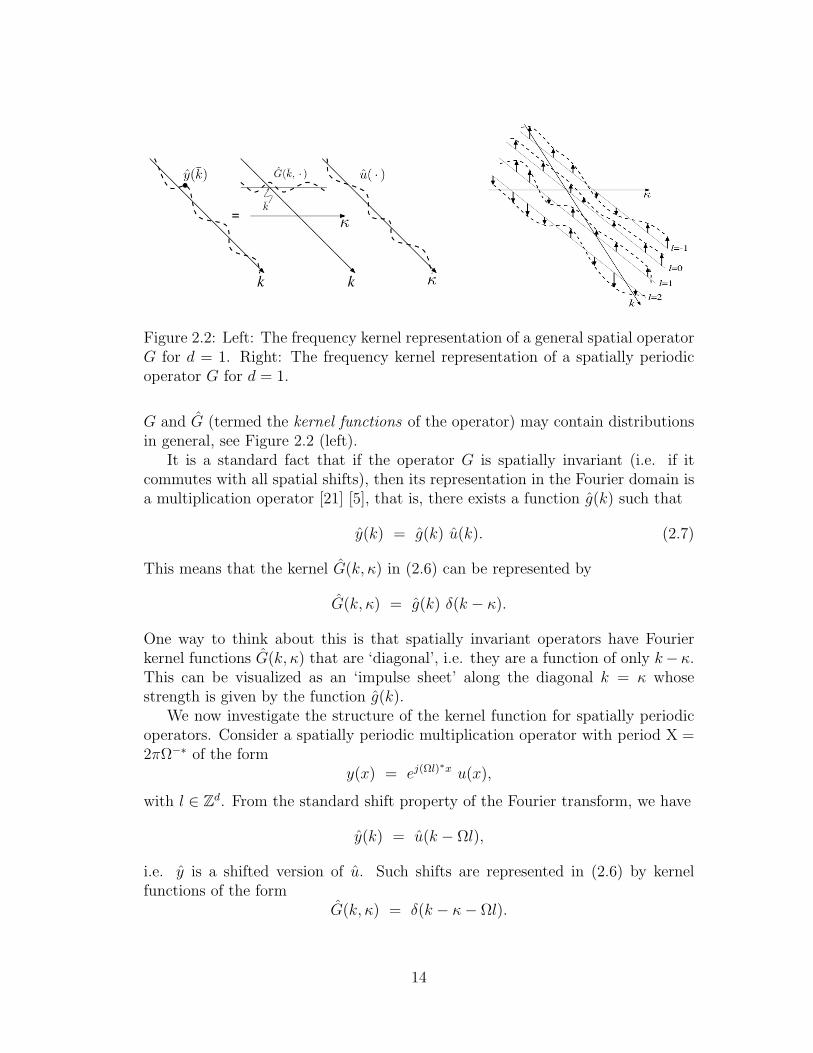
Figure 2.2: Left: The frequency kernel representation of a general spatial operatorG for d = 1. Right: The frequency kernel representation of a spatially periodicoperator G for d = 1.
G and G (termed the kernel functions of the operator) may contain distributionsin general, see Figure 2.2 (left).
It is a standard fact that if the operator G is spatially invariant (i.e. if itcommutes with all spatial shifts), then its representation in the Fourier domain isa multiplication operator [21] [5], that is, there exists a function g(k) such that
y(k) = g(k) u(k). (2.7)
This means that the kernel G(k,) in (2.6) can be represented by
G(k,) = g(k) �(k � ).
One way to think about this is that spatially invariant operators have Fourierkernel functions G(k,) that are ‘diagonal’, i.e. they are a function of only k� .This can be visualized as an ‘impulse sheet’ along the diagonal k = whosestrength is given by the function g(k).
We now investigate the structure of the kernel function for spatially periodicoperators. Consider a spatially periodic multiplication operator with period X =2⇡⌦�⇤ of the form
y(x) = ej(⌦l)⇤x u(x),
with l 2 Zd. From the standard shift property of the Fourier transform, we have
y(k) = u(k � ⌦l),
i.e. y is a shifted version of u. Such shifts are represented in (2.6) by kernelfunctions of the form
G(k,) = �(k � � ⌦l).
14
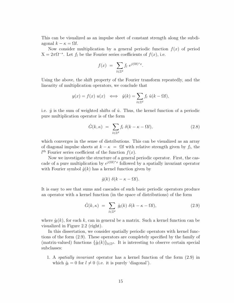
This can be visualized as an impulse sheet of constant strength along the subdi-agonal k � = ⌦l.
Now consider multiplication by a general periodic function f(x) of periodX = 2⇡⌦�⇤. Let f
l
be the Fourier series coe�cients of f(x), i.e.
f(x) =X
l2Zd
fl
ej(⌦l)⇤x.
Using the above, the shift property of the Fourier transform repeatedly, and thelinearity of multiplication operators, we conclude that
y(x) = f(x) u(x) () y(k) =X
l2Zd
fl
u(k � ⌦l),
i.e. y is the sum of weighted shifts of u. Thus, the kernel function of a periodicpure multiplication operator is of the form
G(k,) =X
l2Zd
fl
�(k � � ⌦l), (2.8)
which converges in the sense of distributions. This can be visualized as an arrayof diagonal impulse sheets at k � = ⌦l with relative strength given by f
l
, thelth Fourier series coe�cient of the function f(x).
Now we investigate the structure of a general periodic operator. First, the cas-cade of a pure multiplication by ej(⌦l)⇤x followed by a spatially invariant operatorwith Fourier symbol g(k) has a kernel function given by
g(k) �(k � � ⌦l).
It is easy to see that sums and cascades of such basic periodic operators producean operator with a kernel function (in the space of distributions) of the form
G(k,) =X
l2Zd
gl
(k) �(k � � ⌦l), (2.9)
where gl
(k), for each k, can in general be a matrix. Such a kernel function can bevisualized in Figure 2.2 (right).
In this dissertation, we consider spatially periodic operators with kernel func-tions of the form (2.9). These operators are completely specified by the family of(matrix-valued) functions {g
l
(k)}l2Zd . It is interesting to observe certain special
subclasses:
1. A spatially invariant operator has a kernel function of the form (2.9) inwhich g
l
= 0 for l 6= 0 (i.e. it is purely ‘diagonal’).
15
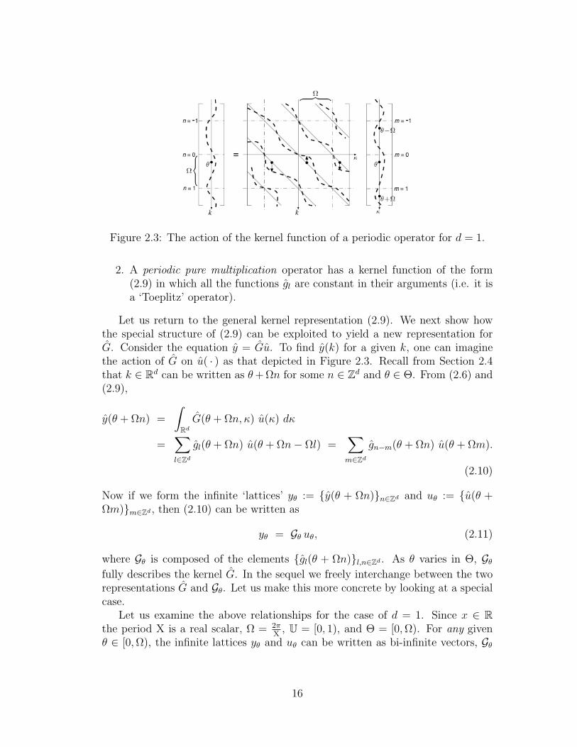
Figure 2.3: The action of the kernel function of a periodic operator for d = 1.
2. A periodic pure multiplication operator has a kernel function of the form(2.9) in which all the functions g
l
are constant in their arguments (i.e. it isa ‘Toeplitz’ operator).
Let us return to the general kernel representation (2.9). We next show howthe special structure of (2.9) can be exploited to yield a new representation forG. Consider the equation y = Gu. To find y(k) for a given k, one can imaginethe action of G on u( · ) as that depicted in Figure 2.3. Recall from Section 2.4that k 2 Rd can be written as ✓+ ⌦n for some n 2 Zd and ✓ 2 ⇥. From (2.6) and(2.9),
y(✓ + ⌦n) =
Z
Rd
G(✓ + ⌦n,) u() d
=X
l2Zd
gl
(✓ + ⌦n) u(✓ + ⌦n� ⌦l) =X
m2Zd
gn�m
(✓ + ⌦n) u(✓ + ⌦m).
(2.10)
Now if we form the infinite ‘lattices’ y✓
:= {y(✓ + ⌦n)}n2Zd and u
✓
:= {u(✓ +⌦m)}
m2Zd , then (2.10) can be written as
y✓
= G✓
u✓
, (2.11)
where G✓
is composed of the elements {gl
(✓ + ⌦n)}l,n2Zd . As ✓ varies in ⇥, G
✓
fully describes the kernel G. In the sequel we freely interchange between the tworepresentations G and G
✓
. Let us make this more concrete by looking at a specialcase.
Let us examine the above relationships for the case of d = 1. Since x 2 Rthe period X is a real scalar, ⌦ = 2⇡
X, U = [0, 1), and ⇥ = [0, ⌦). For any given
✓ 2 [0, ⌦), the infinite lattices y✓
and u✓
can be written as bi-infinite vectors, G✓
16
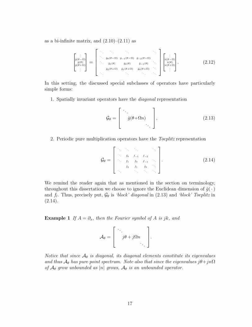
as a bi-infinite matrix, and (2.10)–(2.11) as
2
4
.
.
.
y(✓�⌦)y(✓)
y(✓+⌦).
.
.
3
5 =
2
6
6
6
4
.
.
.
.
.
.
.
.
.
.
.
.
.
.
.
g0(✓�⌦) g�1(✓�⌦) g�2(✓�⌦).
.
.
g1(✓) g0(✓) g�1(✓).
.
.
g2(✓+⌦) g1(✓+⌦) g0(✓+⌦).
.
.
.
.
.
.
.
.
.
.
.
.
.
.
3
7
7
7
5
2
4
.
.
.
u(✓�⌦)u(✓)
u(✓+⌦).
.
.
3
5. (2.12)
In this setting, the discussed special subclasses of operators have particularlysimple forms:
1. Spatially invariant operators have the diagonal representation
G✓
=
2
6
4
.
.
.
g(✓+⌦n).
.
.
3
7
5
, (2.13)
2. Periodic pure multiplication operators have the Toeplitz representation
G✓
=
2
6
6
6
4
.
.
.
.
.
.
.
.
.
.
.
.
.
.
.
f0 f�1 f�2.
.
.
f1 f0 f�1.
.
.
f2 f1 f0.
.
.
.
.
.
.
.
.
.
.
.
.
.
.
3
7
7
7
5
. (2.14)
We remind the reader again that as mentioned in the section on terminology,throughout this dissertation we choose to ignore the Euclidean dimension of g( · )and f
l
. Thus, precisely put, G✓
is ‘block’ diagonal in (2.13) and ‘block’ Toeplitz in(2.14).
Example 1 If A = @x
, then the Fourier symbol of A is jk, and
A✓
=
2
6
4
.
.
.
j✓ + j⌦n
.
.
.
3
7
5
.
Notice that since A✓
is diagonal, its diagonal elements constitute its eigenvaluesand thus A
✓
has pure point spectrum. Note also that since the eigenvalues j✓+jn⌦of A
✓
grow unbounded as |n| grows, A✓
is an unbounded operator.
17

Figure 2.4: Graphical interpretation of G✓
for d = 1 and ✓ 2 [0, ⌦). Note that ✓need only change in [0, ⌦) to fully capture G.
If f(x) = cos(⌦x), then f(x) = 12(ej⌦x + e�j⌦x), and
F =1
2
2
6
6
6
6
4
.
.
.
.
.
.
.
.
. 0 1
1 0.
.
.
.
.
.
.
.
.
3
7
7
7
7
5
,
where we have dropped the ✓ subscript in F as it is independent of this variable.
Remark 1 Another way to interpret the new representation introduced above isto think of G
✓
, for every given ✓, as a ‘sample’ of G; see Figure 2.4. As ✓ changesin ⇥, this ‘sampling grid’ slides on the impulse sheets of G.
Remark 2 As ✓ assumes values in ⇥, one can also interpret u✓
as a lifted (infrequency) version of u( · ) [9,10]. Let M
✓
denote the unitary lifting operator suchthat u
✓
= M✓
u, y✓
= M✓
y, and G✓
= M✓
G M ⇤✓
. We will henceforth refer to thisrepresentation of functions and operators as the lifted representation.
Suppose u belongs to a dense subset D of L2(Rd) such that
u 2 D ⇢ L2(Rd) =) u✓
2 `2(Zd) for every ✓ 2 ⇥.
Then since M✓
is unitary and therefore preserves norms,
kuk2L
2 =
Z
Rd
ku(k)k2 dk =X
m2Zd
Z
⇥
ku(✓ + ⌦m)k2 d✓ =
Z
⇥
ku✓
k2`
2 d✓,
where k · k is the standard Euclidean norm. We also have
X
l2Zd
Z
Rd
trace[gl
(k) g⇤l
(k)] dk =
Z
⇥
trace[G✓
G⇤✓
] d✓ =
Z
⇥
kG✓
k2HS d✓, (2.15)
18

with kTk2HS := trace[T T ⇤] being the square of the Hilbert-Schmidt norm1 of T .
Remark 3 It is well known that the trace of a finite-dimensional matrix is equalto the sum of the elements on its main diagonal. This easily extends to the caseof operators on `2(Z), which can be thought of as infinite-dimensional matrices.But it may not be obvious what is meant by the trace of an operator on `2(Zd).Since we will often use the notion of the trace of such operators in this work, itis worth mentioning here that the trace has a more fundamental definition. If{e
i
}i2Zd denotes an orthonormal basis of `2(Zd), then for those operators T on
`2(Zd) for which the following quantity is finite we have trace[T ] =P
i2Zd
e⇤i
T ei
[20].
Remark 4 From the unitary property of M✓
it follows that G is a bounded oper-ator if and only if G
✓
is a bounded operator for all ✓ 2 ⇥.
For a di↵erent method of deriving the representations (2.13)–(2.14) we referthe reader to [22] [23].
2.5.2 Spectral-Correlation Density Operators
Let u(x) be a wide-sense stationary random field. We define its Fourier transformas u(k) =
R
Rd
e�jk
⇤x u(x) dx.2 Let Ru = E {u(x) u⇤(�)}. Then it follows that
Su(k,) := E {u(k) u⇤()} (2.16)
=
Z
Rd
Z
Rd
e�j(k⇤x�
⇤�) Ru(x,�) d� dx.
Su is the Fourier transform of Ru and is called the spectral-correlation density of u.Notice that Su is a function of two variables, as opposed to the (power) spectraldensity function which is a function of only one frequency variable.
Since the random field u is wide-sense stationary, we have Ru(x,�) = Ru(x��). Therefore from (2.16) the spectral-correlation density of u assumes the form
Su(k,) = Su
0 (k) �(k � ),
where Su
0 (k) is the (power) spectral density of u. Heuristically, the above equationmeans that u is an irregular function of frequency in a way that no two samplesu(k) and u(), k 6= , of u are correlated [12].
1The Hilbert-Schmidt norm of an operator is a generalization of the Frobenius norm of finite-dimensional matrices kAk2
F
=P
m,n
|amn
|2 = trace[AA
⇤].2Technically, the sample paths of wide-sense stationary signals are persistent and not finite-
energy functions [12] and hence their Fourier transforms fail to exist, i.e.,R
x2Rd e
�jk
⇤x
u(x) dx
does not converge as a quadratic-mean integral. This problem can be circumvented by intro-ducing the integrated Fourier transform [12] [24]. We will proceed formally and not pursue thisdirection here.
19

Next we consider a wide-sense cyclostationary random field u(x) whose auto-correlation satisfies (2.5). The next theorem describes the structure of Su.
Theorem 1 Let u be a wide-sense cyclostationary random field with autocorrela-tion Ru(x,�) = Ru(x+Xm,�+Xm), m 2 Zd. Then u has the spectral-correlationdensity
Su(k,) =X
l2Zd
Su
l
(k) �(k � � ⌦l) (2.17)
for some family of functions Su
l
, l 2 Zd.
Proof: See Appendix.
Thus for a general cyclostationary signal the spectral-correlation density, as an op-erator in the Fourier domain, can be visualized as in Figure 2.2 (right). Equation(2.17) implies that u(k) has only nonzero correlation with the samples u(k�⌦l),l 2 Zd, with Su
l
(k) characterizing the amount of correlation. Hence in contrast tostationary signals, di↵erent frequency components of cyclostationary signals arecorrelated.
The following change of variables gives Su a more transparent interpretation[25]
(
µ := k �
{ :=k +
2
=)⇢
k = { + µ
2
= { � µ
2
Essentially, µ characterizes the (continuum of) subdiagonals of Su and { deter-mines the position on the µth subdiagonal, as demonstrated in Figure 2.5 (left).Let us define
Qu({, µ) := E�
u({ +µ
2) u⇤({ � µ
2)
. (2.18)
From (2.16), (2.17), and (2.18) it follows that
Qu({, µ) =
⇢
Su
l
(k) µ = ⌦l, l 2 Zd,0 otherwise.
(2.19)
In words, Qu({, µ) is zero unless µ is such that Qu({, µ) lands on one of theimpulse sheets Su
l
( · ). Let us see what this means in terms of u. Notice from(2.18) and (2.19) that for a general cyclostationary signal u, Qu({, µ) is onlynonzero if the samples u({ + µ
2) and u⇤({ � µ
2) of u are a distance µ = ⌦l apart
for some l 2 Zd; see Figure 2.5 (right). Once such a µ is reached, Qu({, µ) shows
20

Figure 2.5: Graphical interpretation of Qu({, µ) for d = 1.
Figure 2.6: Composition of spatially periodic operators in the frequency domainfor d = 1.
the amount of correlation between all such sample-pairs of u as { varies.3
Finally, the spectral-correlation density of the output of a periodic operatorwith a cyclostationary input, y = Gu, is given by
Sy(k,) = E {y(k) y⇤()} = E��
Gu�
(k)�
Gu�⇤
()
= En
Z
Rd
Z
Rd
G(k,1) u(1) u⇤(2) G⇤(2,) d1 d2
o
=
Z
Rd
Z
Rd
G(k,1) Su(1,2) G⇤(2,) d1 d2
=�
G Su G⇤�(k,), (2.20)
where Su(1,2) := E {u(1) u⇤(2)}, and G Su G⇤ indicates the ‘composition’ ofkernels. It is possible to show that periodic kernels (with a common period) areclosed under addition and composition. Hence from (2.9), (2.17), and (2.20), itfollows that Sy too is a periodic kernel. It is helpful to visualize the compositionSy = G Su G⇤ as shown in Figure 2.6. Such a kernel composition in d = 1 can bethough of as an extended form of matrix multiplication where the matrix elementsare characterized by the continuously-varying indices k, . Of course if u is a wide-sense stationary random field and/or G is a spatially invariant operator, then Su
and/or G will become a diagonal operator in Figure 2.6. Finally the composition
3Compare this with the case of wide-sense stationary signals where S
u is diagonal and henceQ
u({, µ) = 0 for all µ 6= 0, i.e. u({) is not correlated to any sample other than itself.
21
defined by (2.20) can also be represented in the lifted representation by
Sy
✓
= G✓
Su
✓
G⇤✓
. (2.21)
2.6 Representations of Spatially Periodic Sys-tems
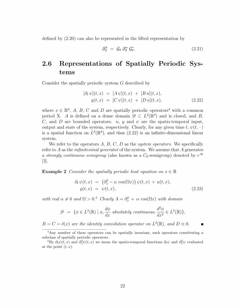
Consider the spatially periodic system G described by
[@t
](t, x) = [A ](t, x) + [B u](t, x),
y(t, x) = [C ](t, x) + [D u](t, x), (2.22)
where x 2 Rd, A, B, C and D are spatially periodic operators4 with a commonperiod X. A is defined on a dense domain D ⇢ L2(Rd) and is closed, and B,C, and D are bounded operators. u, y and are the spatio-temporal input,output and state of the system, respectively. Clearly, for any given time t, (t, · )is a spatial function on L2(Rd), and thus (2.22) is an infinite-dimensional linearsystem.
We refer to the operators A, B, C, D as the system operators. We specificallyrefer to A as the infinitesimal generator of the system. We assume that A generatesa strongly continuous semigroup (also known as a C0-semigroup) denoted by eAt
[3].
Example 2 Consider the spatially periodic heat equation on x 2 R
@t
(t, x) =�
@2x
� ↵ cos(⌦x)�
(t, x) + u(t, x),
y(t, x) = (t, x), (2.23)
with real ↵ 6= 0 and ⌦ > 0.5 Clearly A = @2x
+ ↵ cos(⌦x) with domain
D = {� 2 L2(R) | �,d�
dxabsolutely continuous,
d2�
dx22 L2(R)},
B = C = �(x) are the identity convolution operator on L2(R), and D ⌘ 0.
4Any number of these operators can be spatially invariant, such operators constituting asubclass of spatially periodic operators.
5By @
t
(t, x) and @
2
x
(t, x) we mean the spatio-temporal functions @t
and @
2
x
evaluatedat the point (t, x).
22

The system (2.22) can also be represented by a spatio-temporal kernel G,
y(t, x) =�
Gu�
(t, x)
=
Z
Rd
Z 1
0
G(t, ⌧ ; x,�) u(⌧,�) d⌧ d�,
where G satisfies
G(t, ⌧ ; x,�) = G(t� ⌧ ; x,�), (2.24)
G(t, ⌧ ; x + Xm,�+ Xm) = G(t, ⌧ ; x,�), (2.25)
for all t � ⌧ � 0 and all x,� 2 Rd, with an abuse of notation in using G in (2.24)to represent both the kernel and the temporal impulse response of the system.
On the other hand, one could apply the spatial Fourier transform to both sidesof (2.22) to get
[@t
](t, k) = [A ](t, k) + [B u](t, k),
y(t, k) = [C ](t, k) + [D u](t, k), (2.26)
with k 2 Rd. This system corresponds to the kernel
G(t, ⌧ ; k,) = G(t� ⌧ ; k,), (2.27)
G(t, ⌧ ; k,) =X
l2Zd
Gl
(t, ⌧ ; k) �(k � � ⌦l), (2.28)
for all t � ⌧ � 0 and k, 2 Rd. Notice that for any given t, G(t; · , · ) is a Fourierkernel of the form illustrated in Figure 2.2. Applying the lifting transform to bothsides of (2.26) we have
[@t
✓
](t) = [A✓
✓
](t) + [B✓
u✓
](t),
y✓
(t) = [C✓
✓
](t) + [D✓
u✓
](t), (2.29)
with ✓ 2 ⇥. The impulse response of (2.29) has the form
G✓
(t) = C✓
eA✓
t B✓
+ D✓
. (2.30)
Finally, the transfer functions of the systems (2.22), (2.26), (2.29), correspondrespectively to
G(!) := C (j!I � A)�1B + D,
G(!) := C (j!I � A)�1B + D,
G✓
(!) := C✓
(j!I �A✓
)�1B✓
+ D✓
.
23

Figure 2.7: Relationship between di↵erent representations of the spatio-temporalsystem G. F
x
is the spatial Fourier transfom, and Ft
the temporal Fourier trans-form. M
✓
is the frequency lifiting operator.
Figure 2.7 summarizes the notational conventions used in this work.Example 2 continued Let us return to the example of the periodic heat
equation on the real line described by (2.23). Rewriting the system in its liftedrepresentation we have
@t
✓
(t) = A✓
✓
(t) + B✓
u✓
(t),
y✓
(t) = C✓
✓
(t) + D✓
u✓
(t), (2.31)
with ✓ 2 [0, ⌦), where from Example 1 of Section 2.5
A✓
=
2
6
6
4
. . .�(✓ + ⌦n)2
. . .
3
7
7
5
� ↵
2
2
6
6
6
6
4
.
.
.
.
.
.
.
.
. 0 1
1 0.
.
.
.
.
.
.
.
.
3
7
7
7
7
5
, (2.32)
B✓
= C✓
=
2
6
6
4
. . .1
. . .
3
7
7
5
, D✓
⌘ 0, (2.33)
G✓
(!) = C✓
(j!I �A✓
)�1B✓
+ D✓
=
2
6
6
6
6
6
6
6
4
.
.
.
.
.
.
.
.
.
.
.
.
↵/2
↵/2 j!+(✓+⌦n)2 ↵/2
↵/2.
.
.
.
.
.
.
.
.
.
.
.
3
7
7
7
7
7
7
7
5
�1
.
(2.34)
Notice that (2.31)–(2.34) is now fully decoupled in the variable ✓. In other words,(2.23) is equivalent to the family of state-space representations (2.31)–(2.33) pa-
24

Figure 2.8: Left: A spatially periodic system, as the closed-loop interconnectionof a spatially invariant system Go and a spatially periodic operator F . Right: Aspatially periodic system can be written as the LFT of a system Go with spatiallyinvariant dynamics and a spatially periodic operator F .
rameterized by ✓ 2 [0, ⌦).
Remark 5 An advantage of the lifted representation is that it allows for (2.31)to be treated like a multivarible system (under minor technical assumptions). It isthen possible to extend many existing tools from linear systems theory to (2.31).For example Chapter 4 generalizes the Nyquist criterion to determine the sta-bility of (2.31), Chapter 5 uses the algebraic Lyapunov equation to calculate theH2-norm of G, and Chapter 6 employes Gersgorin-like arguments to locate thespectrum of A
✓
. Also [22] [26] use the lifted representation to investigate theoccurrence of parametric resonance in spatially periodic systems.
Remark 6 It is interesting to note that (2.23) can be written as the feedbackinterconnection of the spatially invariant system Go
@t
(t, x) = @2x
(t, x) + w(t, x),
y(t, x) = (t, x),
and the (memoryless) spatially periodic multiplication operator F (x) = �↵ cos(⌦x),
w(t, x) = � ↵ cos(⌦x) y(t, x) + u(t, x),
as in Figure 5.1 (left).More generally, a wide class of spatially periodic systems can be written as
the LFT (linear fractional transformation [27]) of a spatially periodic system withspatially invariant dynamics, and a bounded spatially periodic pure multiplicationoperator. To be more concrete, the spatially periodic system
@t
(t, x) = A (t, x) + B u(t, x),
y(t, x) = C (t, x) + D u(t, x),
25

can be considered as
@t
(t, x) =�
Ao + Bo F Co
�
(t, x) + B u(t, x),
y(t, x) = C (t, x) + D u(t, x), (2.35)
where the (possibly unbounded) operators Ao, Bo, Co are spatially invariant, thebounded operators B, C, D are spatially periodic, and F is a bounded spatiallyperiodic pure multiplication operator. Ao, Bo, Co and E := Bo F Co are all definedon a dense domain D ⇢ L2(R). Finally, (2.35) corresponds to the LFT of thesystem
Go =
2
6
4
Ao B Bo
C D 0Co 0 0
3
7
5
and the operator F , as shown Figure 5.1 (right).
Finally, the spectral-correlation density of the output y of a linear spatiallyperiodic system G with input u is given by
Ry(t, ⌧ ;k,) = E {y(t, k) y⇤(⌧,)} = E��
Gu�
(t, k)�
Gu�⇤
(⌧,)
= En
Z
G(t, ⌧1; k,1) u(⌧1,1) u⇤(⌧2,2) G⇤(⌧2, ⌧ ;2,) d1 d2 d⌧1 d⌧2o
=
Z
G(t, ⌧1; k,1) Ru(⌧1, ⌧2;1,2) G⇤(⌧2, ⌧ ;2,) d1 d2 d⌧1 d⌧2
=�
G Ru G⇤�(t, ⌧ ; k,), (2.36)
where Ru(⌧1, ⌧2;1,2) := E {u(⌧1,1) u⇤(⌧2,2)}. If u is taken to be wide-sensestationary in the temporal direction and wide-sense cyclostationary in the spatialdirection, then
Ru(t, ⌧ ; k,) = Ru(t� ⌧ ; k,), (2.37)
Ru(t, ⌧ ; k,) =X
l2Zd
Ru
l
(t, ⌧ ; k) �(k � � ⌦l), (2.38)
for all t � ⌧ � 0 and k, 2 Rd. Comparing (2.37)–(2.38) and (2.27)–(2.28), itis clear that in (2.36) the operators G, Ru and G⇤ are all spatially periodic witha common period and have the same structure. Hence, by the closedness undercompositions of such operators, Ry will inherit the same structure and we have
Ry(t, ⌧ ; k,) = Ry(t� ⌧ ; k,), (2.39)
Ry(t, ⌧ ; k,) =X
l2Zd
Ry
l
(t, ⌧ ; k) �(k � � ⌦l). (2.40)
26

2.7 Appendix to Chapter 2
Proof of Theorem 1
From Ru(x,�) = Ru(x + Xm,�+ Xm) and using ⇠ := x� � we have
Ru(x,�) = Ru(�+ ⇠,�) = Ru(�+ Xm + ⇠,�+ Xm),
which means that Ru(�+ ⇠,�) is periodic in � and hence admits a Fourier seriesexpansion
Ru(�+ ⇠,�) =X
l2Zd
rl
(⇠) ej(⌦l)⇤�.
Thus Ru(x,�) =P
l
rl
(x��) ej(⌦l)⇤�. Substituting in (2.16) and using the changeof variables � := k � ,
Su(k,) =
Z
Rd
Z
Rd
e�j(k⇤x�
⇤�) Ru(x,�) dx d�
=
Z
Rd
Z
Rd
e�j�
⇤� e�jk
⇤(x��)X
l2Zd
rl
(x� �) ej(⌦l)⇤� dx d�
=X
l2Zd
Z
Rd
e�j�
⇤�+j(⌦l)⇤�
Z
Rd
e�jk
⇤(x��) rl
(x� �) dx d�
=X
l2Zd
Z
Rd
e�j(��⌦l)⇤� Su
l
(k) d� =X
l2Zd
Su
l
(k) �(k � � ⌦l),
where Su
l
( · ) is the Fourier transform of rl
( · ).
27

Chapter 3
Norms of Spatially PeriodicSystems
Does anyone believe that the di↵erence between the Lebesgue and Riemann inte-grals can have physical significance, and that whether say, an airplane would orwould not fly could depend on this di↵erence? If such were claimed, I should notcare to fly in that plane. R. W. Hamming
3.1 Introduction
In this chapter we introduce the notion of the H2- and H1-norms for spatiallyperiodic systems, and give both deterministic and stochastic interpretations ofour definition for the H2-norm. To motivate this, we first examine the definitionof these norms for the case of spatially periodic operators, which we denote byH2
sp and H1sp . Again the bi-infinite matrix representation (i.e., the frequency lifted
representation) plays a central role in allowing us to extend methods from standardlinear systems theory to compute the norms of spatially periodic systems. Thisrepresentation is also used to discuss truncations and the numerical calculation ofnorms. We finish the chapter with some examples. Throughout this chapter, it isalways assumed that the spatially periodic system G is exponentially stable.
Notation: We shall denote by G the system described by (2.22) but withD ⌘ 0, i.e., G = G + D. Clearly, all the statements and definitions made for Gtherein apply equally to G, mutatis mutandis. We also define Ry to be the outputautocorrelation of the system G given an input with autocorrelation Ru.
28
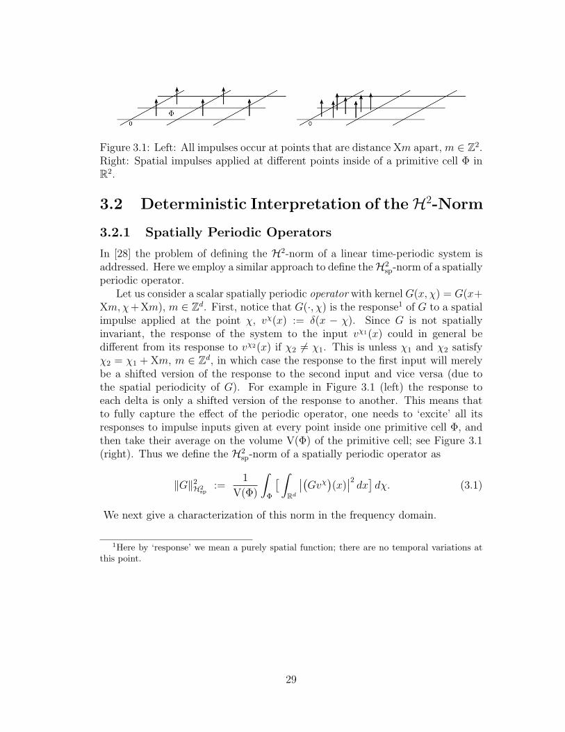
Figure 3.1: Left: All impulses occur at points that are distance Xm apart, m 2 Z2.Right: Spatial impulses applied at di↵erent points inside of a primitive cell � inR2.
3.2 Deterministic Interpretation of the H2-Norm
3.2.1 Spatially Periodic Operators
In [28] the problem of defining the H2-norm of a linear time-periodic system isaddressed. Here we employ a similar approach to define theH2
sp-norm of a spatiallyperiodic operator.
Let us consider a scalar spatially periodic operator with kernel G(x,�) = G(x+Xm,�+Xm), m 2 Zd. First, notice that G(·,�) is the response1 of G to a spatialimpulse applied at the point �, v�(x) := �(x � �). Since G is not spatiallyinvariant, the response of the system to the input v�1(x) could in general bedi↵erent from its response to v�2(x) if �2 6= �1. This is unless �1 and �2 satisfy�2 = �1 + Xm, m 2 Zd, in which case the response to the first input will merelybe a shifted version of the response to the second input and vice versa (due tothe spatial periodicity of G). For example in Figure 3.1 (left) the response toeach delta is only a shifted version of the response to another. This means thatto fully capture the e↵ect of the periodic operator, one needs to ‘excite’ all itsresponses to impulse inputs given at every point inside one primitive cell �, andthen take their average on the volume V(�) of the primitive cell; see Figure 3.1(right). Thus we define the H2
sp-norm of a spatially periodic operator as
kGk2H2
sp:=
1
V(�)
Z
�
⇥
Z
Rd
�
�
�
Gv�
�
(x)�
�
2dx⇤
d�. (3.1)
We next give a characterization of this norm in the frequency domain.
1Here by ‘response’ we mean a purely spatial function; there are no temporal variations atthis point.
29

Theorem 2 If G is a scalar spatially periodic operator, we have
kGk2H2
sp:=
1
V(�)
Z
�
Z
Rd
|G(x,�)|2 dx d� (3.2)
=1
2⇡
X
l2Zd
Z
Rd
|Gl
(k)|2 dk (3.3)
=1
2⇡
Z
⇥
trace[G✓
G⇤✓
] d✓. (3.4)
Proof: See Appendix.
Notice that (3.3) is nothing but the integral of the amplitudes of all the impulsesheets G
l
. Also, comparing (3.4) and (2.15) we have kGk2H2
sp= 1
2⇡
R
⇥kG
✓
k2HS d✓.
3.2.2 Linear Spatially Periodic Systems
Now consider a scalar linear spatially periodic system described by its kernelG(t� ⌧ ; x,�) which satisfies (2.24)–(2.25), and let us assume for now that D ⌘ 0.Inspired by the discussions of the previous subsection we define
kGk2H2 :=
1
V(�)
Z
�
Z
Rd
Z 1
0
|G(t; x,�)|2 dt dx d�.
This definition can be interpreted as
kGk2H2 =
1
V(�)
Z
�
Z
Rd
Z 1
0
�
�
�
Gu�
�
(t, x)�
�
2dt dx d�,
where u�(t, x) := w(t) v�(x) = �(t) �(x � �) [29].2 Hence for an exponentiallystable MIMO (multi-input multi-output) system G with D 6= 0, the appropriatedefinition of the H2-norm is given by
kGk2H2 := kGk2
H2 + kDk2H2
sp
=1
V(�)
Z
�
Z
Rd
Z 1
0
trace[G(t; x,�) G⇤(t;�, x)] dt dx d� + kDk2H2
sp.
(3.5)
Notice that if a spatially periodic system G has no temporal dynamics (i.e. itis a memoryless system), it becomes a purely spatial one G = D, where D is aspatially periodic operator. Thus kGk2
H2 = 0 and one employs the arguments ofthe previous subsection to find kGk2
H2 = kDk2H2
sp. It is also interesting to view the
H2-norm in the spatial-frequency domain.
2We have used the fact that G is time-invariant and thus �(t) is enough to capture its completetemporal response.
30
Theorem 3 Consider the exponentially stable spatially periodic system G withG
✓
(t) = C✓
eA✓
t B✓
+ D✓
. If kGk2H2 as defined in (3.5) exists and is finite, then
kGk2H2 =
1
2⇡
Z
⇥
Z 1
0
trace[G✓
(t)G⇤✓
(t)] dt d✓ + kDk2H2
sp
=1
4⇡2
Z
⇥
Z 1
�1trace[G
✓
(!) G⇤✓
(!)] d! d✓ + kDk2H2
sp
=1
4⇡2
Z 1
�1
X
l2Zd
Z
Rd
trace[Gl
(!; k) G⇤l
(!; k)] dk d! + kDk2H2
sp.
In addition,
kGk2H2 =
1
2⇡
Z
⇥
trace[C✓
P✓
C⇤✓
] d✓+kDk2H2
sp=
1
2⇡
Z
⇥
trace[B⇤✓
Q✓
B✓
] d✓+kDk2H2
sp,
where P✓
and Q✓
are the solutions of the (✓-parameterized) algebraic Lyapunovequations
A✓
P✓
+ P✓
A⇤✓
= �B✓
B⇤✓
, A⇤✓
Q✓
+ Q✓
A✓
= �C⇤✓
C✓
. (3.6)
Proof: See Appendix.
Remark 7 It is known that for spatially distributed systems in dimensions d � 2,exponential stability is not enough to guarantee finiteness of the H2-norm [30]. Wewill see an example of such a system in Section 3.6. Theorem 9 in the Appendixgives a su�cient condition for the the H2-norm to be finite in any spatial dimen-sion.
3.3 Stochastic Interpretation of the H2-Norm
3.3.1 Spatially Periodic Operators
Consider a scalar spatially periodic operator with Fourier kernel
G(k,) =X
l2ZR
Gl
(k) �(k � � ⌦l).
Assume that G is fed with a wide-sense stationary spatial random field v(x) withautocorrelation Rv(x��) and spectral-correlation density Sv(k,) = Sv
0 (k) �(k�), where Sv
0 (k) is the spectral density of v. Then as seen in Section 2.5.2 theoutput y(x) =
�
Gv�
(x) will have the spectral-correlation density
Sy = G Sv G⇤,
31
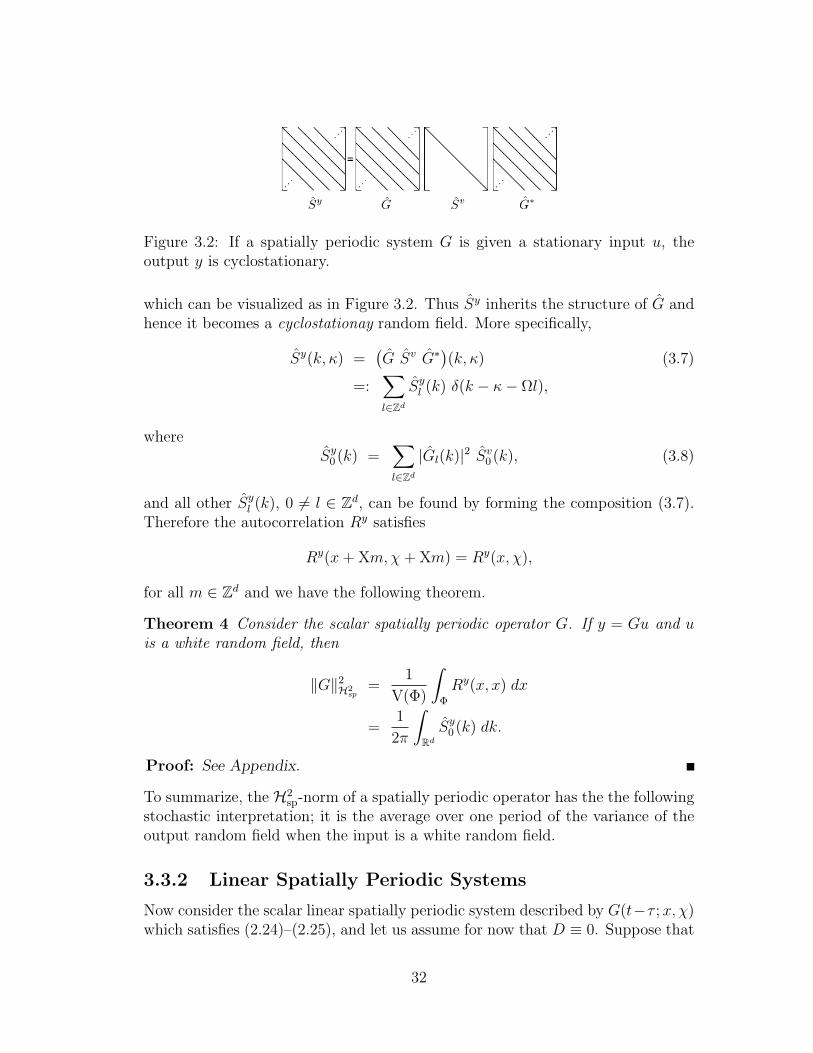
Figure 3.2: If a spatially periodic system G is given a stationary input u, theoutput y is cyclostationary.
which can be visualized as in Figure 3.2. Thus Sy inherits the structure of G andhence it becomes a cyclostationay random field. More specifically,
Sy(k,) =�
G Sv G⇤�(k,) (3.7)
=:X
l2Zd
Sy
l
(k) �(k � � ⌦l),
whereSy
0 (k) =X
l2Zd
|Gl
(k)|2 Sv
0 (k), (3.8)
and all other Sy
l
(k), 0 6= l 2 Zd, can be found by forming the composition (3.7).Therefore the autocorrelation Ry satisfies
Ry(x + Xm,�+ Xm) = Ry(x,�),
for all m 2 Zd and we have the following theorem.
Theorem 4 Consider the scalar spatially periodic operator G. If y = Gu and uis a white random field, then
kGk2H2
sp=
1
V(�)
Z
�
Ry(x, x) dx
=1
2⇡
Z
Rd
Sy
0 (k) dk.
Proof: See Appendix.
To summarize, the H2sp-norm of a spatially periodic operator has the the following
stochastic interpretation; it is the average over one period of the variance of theoutput random field when the input is a white random field.
3.3.2 Linear Spatially Periodic Systems
Now consider the scalar linear spatially periodic system described by G(t�⌧ ; x,�)which satisfies (2.24)–(2.25), and let us assume for now that D ⌘ 0. Suppose that
32
the system is given an input u(t, x) which is a wide-sense stationary random fieldin both the temporal and the spatial directions, with autocorrelation function
Ru(t, ⌧ ; x,�) = Ru(t� ⌧ ; x,�),
Ru(t, ⌧ ; x,�) = Ru(t, ⌧ ; x� �),
for all t � ⌧ � 0 and x,� 2 Rd. By what has been shown in the precedingsubsection, we know that the output of the system y(t, x) =
�
Gu�
(t, x) is a randomfield with autocorrelation Ry(t, ⌧ ; x,�) that satisfies
Ry(t, ⌧ ; x,�) = Ry(t� ⌧ ; x,�),
Ry(t, ⌧ ; x + Xm,�+ Xm) = Ry(t, ⌧ ; x,�),
for all t � ⌧ � 0, x,� 2 Rd and m 2 Zd. Namely, the output random field remainswide-sense stationary in the temporal direction (due to the time-invariance of G),but inherits the spatial-periodicity of the system and as such becomes a cyclosta-tionary random field in the spatial direction. The above identities are equivalentto those expressed in the spatial frequency domain in (2.39)–(2.40).
It particular, if the input u is a white random field in both the spatial andtemporal directions, Su(!, ⌫; k,) = �(! � ⌫) �(k � ), then
kGk2H2 =
1
V(�)
Z
�
Ry(0; x, x) dx.
Hence for an exponentially stable MIMO system G with D 6= 0, the stochasticinterpretation of the H2-norm would be
kGk2H2 = kGk2
H2 + kDk2H2
sp
=1
V(�)
Z
�
trace[Ry(0; x, x)] dx + kDk2H2
sp
=1
4⇡2
Z 1
�1
Z
Rd
trace[Sy
0(!; k)] dk d! + kDk2H2
sp,
where Sy
is the spatio-temporal Fourier transform of Ry, and one can employ thestochastic methods of the previous subsection to find kDk2
H2sp
.
Remark 8 As mentioned previously, for certain spatial systems in dimensionsd � 2 with white random input the value of the variance Ry(0; x, x) may be infinite[30]. These are systems for which (3.14) is not finite. In such cases the outputrandom field can still be given an interpretation in the sense of distributions [31].Also, one can still compute the two-point correlations Ry(�t; x, x) and Ry(0; x, x+�x), which will be finite for �t 6= 0 and �x 6= 0. We give an example of this inSection 3.6.
33

3.4 The H1-Norm
3.4.1 Spatially Periodic Operators
We define the H1sp-norm of a bounded spatial operator G as its L2-induced norm
kGkL
2/L
2 .
Theorem 5 If G is a bounded spatially periodic operator, then
kGk2H1sp := kGk2
L
2/L
2 = kGk2L
2/L
2 = sup✓2⇥
kG✓
k2`
2/`
2 = sup✓2⇥
sup�2⌃(G⇤
✓
G✓
)
|�|.
Proof: See Appendix.
Example 3 Let us compute the H1sp
-norm of the bounded spatially periodic puremultiplication operator G described by the periodic function F (x) = cos(⌦x). Firstnotice that since G is already a multiplication (i.e. diagonal) operator in thespatial domain, a spatial Fourier transform will not lead to a simplification in thisparticular problem. In fact
kGkL
2/L
2 = supx2R
| cos(⌦x)| = 1.
But for illustrative purposes, let us also calculate this norm in the spatial-frequency domain. G
✓
= F has the form given in Example 1 of Section 2.5. Onecan write F = 1
2R+ 1
2L where R and L are the right- and left-shift operators on
`2, respectively,
R =
2
6
6
6
6
4
.
.
.
.
.
.
.
.
. 0 0
1 0.
.
.
.
.
.
.
.
.
3
7
7
7
7
5
, L =
2
6
6
6
6
4
.
.
.
.
.
.
.
.
. 0 1
0 0.
.
.
.
.
.
.
.
.
3
7
7
7
7
5
.
Clearly, kFk`
2/`
2 12kRk
`
2/`
2 + 12kLk
`
2/`
2. Since R and L are shift operators,they are unitary, and thus kRk
`
2/`
2 = kLk`
2/`
2 = 1, which means that kFk`
2/`
2 1. It is not hard to show that this upper bound is actually achieved, and hencekGk
L
2/L
2 = sup✓2⇥ kG
✓
k`
2/`
2 = 1.Finally we demonstrate that this norm can also be found from the spectrum
of G⇤✓
G✓
. It is not hard to show that ⌃(G⇤✓
G✓
) = ⌃(F⇤F) = [0, 1], and as a resultsup
✓2⇥ sup�2⌃(G⇤
✓
G✓
) |�| = 1.
34

3.4.2 Linear Spatially Periodic Systems
We define the H1-norm of a spatially periodic system G as its spatio-temporalL2-induced norm. In the following, by the spatio-temporal function u 2 L2
L
2(Rd)
we mean that at any given time t, u(t, · ) is a spatial function in L2(Rd) such thatR1
0ku(t, · )k2
L
2(Rd)dt <1. Let u denote the temporal Fourier transform of u, and
Gu the temporal Fourier transform of Gu. We have
kGk2H1 := sup
u2L
2L
2
kGuk2L
2L
2
kuk2L
2L
2
= supu2L
2L
2
kGuk2L
2L
2
kuk2L
2L
2
= sup!2R
kG(!)k2L
2/L
2 .
Notice here that for every given !, G(!) is a spatially periodic operator on L2(Rd).Now for a spatial function v 2 L2(Rd) let v denote the spatial Fourier transformof v, and G(!) v the spatial Fourier transform of G(!) v. Then
sup!2R
kG(!)k2L
2/L
2 = sup!2R
supv2L
2
kG(!) vk2L
2
kvk2L
2
= sup!2R
supv2L
2
kG(!) vk2L
2
kvk2L
2
= sup!2R
sup✓2⇥
supv
✓
2`
2
kG✓
(!) v✓
k2`
2
kv✓
k2`
2
= sup!2R
sup✓2⇥
kG✓
(!)k2`
2/`
2 ,
where again we have used the property that the Fourier and lifting transformspreserve norms. Finally, using Theorem 5,
sup!2R
sup✓2⇥
kG✓
(!)k2`
2/`
2 = sup!2R
sup✓2⇥
sup�2⌃(G⇤
✓
(!)G✓
(!))
|�|.
We have thus proved the following theorem.
Theorem 6 For the exponentially stable spatially periodic system G,
kGk2H1 = sup
!2RkG(!)k2
L
2/L
2 = sup!2R
sup✓2⇥
kG✓
(!)k2`
2/`
2
= sup!2R
sup✓2⇥
sup�2⌃(G⇤
✓
(!)G✓
(!))
|�|.
3.5 Numerical Implementation and Finite Di-mensional Truncations
In order to numerically calculate the H2- or H1-norm of a spatially periodic sys-tem, one has to perform a finite-dimensional truncation of the infinite-dimensionaloperators that describe the system. For example, to calculate the H2-norm via
35
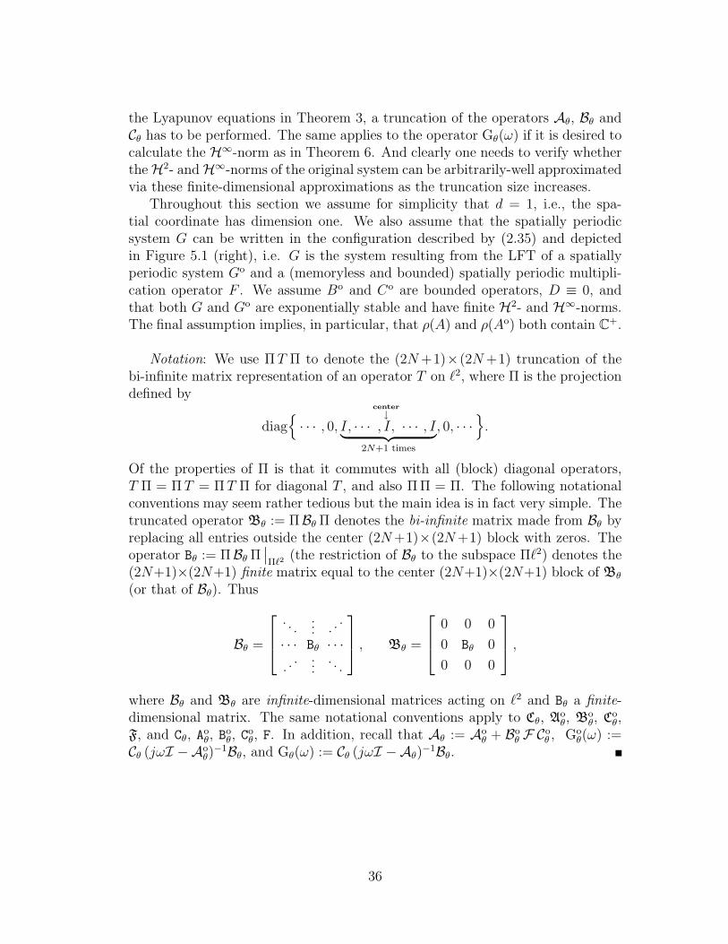
the Lyapunov equations in Theorem 3, a truncation of the operators A✓
, B✓
andC
✓
has to be performed. The same applies to the operator G✓
(!) if it is desired tocalculate the H1-norm as in Theorem 6. And clearly one needs to verify whethertheH2- andH1-norms of the original system can be arbitrarily-well approximatedvia these finite-dimensional approximations as the truncation size increases.
Throughout this section we assume for simplicity that d = 1, i.e., the spa-tial coordinate has dimension one. We also assume that the spatially periodicsystem G can be written in the configuration described by (2.35) and depictedin Figure 5.1 (right), i.e. G is the system resulting from the LFT of a spatiallyperiodic system Go and a (memoryless and bounded) spatially periodic multipli-cation operator F . We assume Bo and Co are bounded operators, D ⌘ 0, andthat both G and Go are exponentially stable and have finite H2- and H1-norms.The final assumption implies, in particular, that ⇢(A) and ⇢(Ao) both contain C+.
Notation: We use ⇧ T ⇧ to denote the (2N +1)⇥(2N +1) truncation of thebi-infinite matrix representation of an operator T on `2, where ⇧ is the projectiondefined by
diagn
· · · , 0, I, · · ·center#
, I, · · · , I| {z }
2N+1 times
, 0, · · ·o
.
Of the properties of ⇧ is that it commutes with all (block) diagonal operators,T ⇧ = ⇧ T = ⇧ T ⇧ for diagonal T , and also ⇧ ⇧ = ⇧. The following notationalconventions may seem rather tedious but the main idea is in fact very simple. Thetruncated operator B
✓
:= ⇧B✓
⇧ denotes the bi-infinite matrix made from B✓
byreplacing all entries outside the center (2N +1)⇥(2N +1) block with zeros. Theoperator B
✓
:= ⇧B✓
⇧�
�
⇧`
2 (the restriction of B✓
to the subspace ⇧`2) denotes the(2N+1)⇥(2N+1) finite matrix equal to the center (2N+1)⇥(2N+1) block of B
✓
(or that of B✓
). Thus
B✓
=
2
6
4
. . .... . .
.
· · · B✓
· · ·. .
. .... . .
3
7
5
, B✓
=
2
6
4
0 0 0
0 B✓
0
0 0 0
3
7
5
,
where B✓
and B✓
are infinite-dimensional matrices acting on `2 and B✓
a finite-dimensional matrix. The same notational conventions apply to C
✓
, Ao✓
, Bo✓
, Co✓
,F, and C
✓
, Ao✓
, Bo✓
, Co✓
, F. In addition, recall that A✓
:= Ao✓
+ Bo✓
F Co✓
, Go✓
(!) :=C
✓
(j!I �Ao✓
)�1B✓
, and G✓
(!) := C✓
(j!I �A✓
)�1B✓
.
36
3.5.1 H1-norm
It is known that a compact operator T 2 B0(`2) can be approximated arbitrarily-well by finite-dimensional matrices [32]. In fact it follows from the definition ofa compact operator that the entries {t
nm
}n,m2Z of the matrix representation of
T decay in all directions such that kT � ⇧ T k`
2/`
2 , kT � T ⇧ k`
2/`
2 , and kT �⇧ T ⇧ k
`
2/`
2 all approach zero as N grows large.The main assumption here is that
sup!2R
k �j!I � Ao(k)��1 k ! 0 as |k|!1. (3.9)
This implies the compactness of the diagonal operator (j!I�Ao✓
)�1 for all ! 2 Rand ✓ 2 [0, ⌦). The fact that compact operators form a two-sided ideal in thealgebra of bounded operators B(`2) and arguments similar to those in the proofof Theorem 9 can now be used to show that (j!I � A
✓
)�1 and G✓
(!) belong toB0(`2) for all ! 2 R and ✓ 2 [0, ⌦). This is the result we were looking for, namely,G
✓
(!) is a compact operator on `2 and as such can be approximated to any degreeof accuracy by ⇧ G
✓
(!) ⇧.But we are still not done. The desired scenario is to only have to compute
G✓
(!) := C✓
(j!I� [Ao✓
+ Bo✓
F Co✓
])�1B✓
,
because only in this case do we have the amenity of dealing with the finite-dimensional matrices A
✓
:= Ao✓
+ Bo✓
F Co✓
, B✓
, and C✓
. Therefore it is importantto find the relationship between ⇧ G
✓
(!) ⇧ and G✓
(!). Notice that we can notdirectly compare C
✓
(j!I � [Ao✓
+ Bo✓
F Co✓
])�1B✓
and C✓
(j!I � Ao✓
+ Bo✓
F Co✓
)�1B✓
because they live on di↵erent operator spaces. Establishing a connection betweenG
✓
(!) and G✓
(!) will be the objective of the next theorem and it is done throughthe use of the truncated operators B
✓
, C✓
, ... , and the transfer function
G✓
(!) := C✓
(j!I � [Ao✓
+ Bo✓
F Co✓
])�1B✓
.
It is important to notice in G✓
(!) that the diagonal operator Ao✓
has not beentruncated. Also, j!I � [Ao
✓
+ Bo✓
F Co✓
] is invertible if and only if j!I � Ao✓
andj!I� [Ao
✓
+ Bo✓
F Co✓
] are invertible.
Remark 9 The di�culty in relating ⇧ G✓
(!) ⇧ to G✓
(!) and G✓
(!) is due to B✓
,C
✓
, F being non-diagonal and ⇧ not commuting with non-diagonal operators. Thisis precisely the reason why ⇧ G
✓
(!) ⇧ 6= G✓
(!). ⇧ G✓
(!) ⇧ is found by composingG
✓
(!) first and then applying ⇧, whereas G✓
(!) is found by applying ⇧ to B✓
, C✓
,Ffirst and then carrying out the composition. These two are in general not equalunless all operators present in the system are diagonal. Indeed, if B
✓
, C✓
, F wereall diagonal, then G
✓
(!) would be diagonal, we would have ⇧ G✓
(!) ⇧ = G✓
(!),
37
and G✓
(!) would be nothing but a diagonal matrix made up of the center 2N +1diagonal elements of G
✓
(!) (or G✓
(!)).
Theorem 7 Consider an exponentially stable spatially periodic system describedby (2.35) with finite H1-norm, and suppose that sup
!2R k�
j!I � Ao(k)��1 k !
0 as |k|!1. Then
sup!2R
sup✓2[0,⌦)
kG✓
(!) � G✓
(!) k ! 0 as N !1.
In particular, if G✓
(!) exists for all ! 2 R and ✓ 2 [0, ⌦), then
sup!2R
sup✓2[0,⌦)
k G✓
(!) k = sup!2R
sup✓2[0,⌦)
kG✓
(!) k ! sup!2R
sup✓2[0,⌦)
kG✓
(!) k
as N !1.
Proof: See Appendix.
The significance of the above theorem is that the H1-norm of G in Theorem 6can now be computed from
kG k2H1 ⇡ sup
!2Rsup
✓2[0,⌦)
k G✓
(!) k,
and one need only deal with the finite-dimensional matrices A✓
, B✓
and C✓
.
3.5.2 H2-norm
For a Hilbert-Schmidt operator T 2 B2(`2) with matrix representation {tmn
}m,n2Z
we haveP1
m,n=�1 |tmn
|2 < 1 [33]. In particular this means that kT � ⇧ T kHS,kT � T ⇧ kHS, and kT � ⇧ T ⇧ kHS all approach zero as N grows large, wherekT k2
HS := trace[T T ⇤]. As opposed to the previous paragraph and the proof ofTheorem 7 where the submultiplicative property of the induced `2 norm plays acentral role, in this paragraph and in the proof of the proceeding Theorem 8 wemake use of the fact that Hilbert-Schmidt operators form a two-sided ideal in thealgebra of bounded operators on `2 [20]. Namely if T0, T1 2 B(`2) and T2 2B2(`2), then T0 T2 T1 2 B2(`2) and kT0 T2 T1 kHS kT0 k
`
2/`
2 kT2 kHS kT1 k`
2/`
2 .The main assumption here is that
Z 1
�1
Z
Rk �j!I � Ao(k)
��1 k2F dk d! < 1,
38

and that Ao( · ) satisfies the regularity conditions given in Theorem 9. Argumentssimilar to those in the proof of Theorem 9 can now be used to show that theoperators (j!I �Ao
✓
)�1, (j!I �A✓
)�1 and G✓
(!) belong to B2(`2) for all ! 2 Rand ✓ 2 [0, ⌦). Therefore G
✓
(!) is a Hilbert-Schmidt operator and as such canbe approximated to any degree of accuracy (in the sense of the Hilbert-Schmidtnorm) by ⇧ G
✓
(!) ⇧.But as in the previous section on the H1-norm, our desired scenario is to only
have to deal with the finite-dimensional systems
G✓
(!) = C✓
(j!I� [Ao✓
+ Bo✓
F Co✓
])�1B✓
.
In particular, we would like to compute the H2-norm by solving Lyapunov equa-tions involving only the finite-dimensiona matrices A
✓
, B✓
, and C✓
. The followingtheorem uses of the truncated systems
G✓
(!) = C✓
(j!I � [Ao✓
+ Bo✓
F Co✓
])�1B✓
.
to establish the connection between G✓
(!) and G✓
(!).
Theorem 8 Consider an exponentially stable spatially periodic system describedby (2.35) with finite H2-norm, and suppose that
R
RR1�1 k
�
j!I�Ao(k)��1k2
F dk d! <1. Then
Z ⌦
0
Z 1
�1kG
✓
(!) � G✓
(!) k2HS d! d✓ ! 0 as N !1.
In particular, if G✓
(!) exists for all ! 2 R and ✓ 2 [0, ⌦), then
Z ⌦
0
Z 1
�1k G
✓
(!) k2F d! d✓ =
Z ⌦
0
Z 1
�1kG
✓
(!) k2HS d! d✓ !
Z ⌦
0
Z 1
�1kG
✓
(!) k2HS d! d✓
as N !1.
Proof: See Appendix.
The significance of the above theorem is that the H2-norm of G can now becomputed from
kG k2H2 ⇡ 1
2⇡
Z ⌦
0
trace[C✓
P✓
C⇤✓
] d✓ =1
2⇡
Z ⌦
0
trace[B⇤✓
Q✓
B✓
] d✓
where P✓
and Q✓
are the solutions of the finite-dimensional Lyapunov equations
A✓
P✓
+ P✓
A⇤✓
= �B✓
B⇤✓
, A⇤✓
Q✓
+ Q✓
A✓
= �C⇤✓
C✓
.
39
Obviously this is much simpler than solving the infinite-dimensional Lyapunovequations (3.6) of Theorem 3.
3.6 Examples
In this section we illustrate how system norms of PDEs can be changed by theintroduction of spatially periodic coe�cients. We also present an example of astable system in two spatial dimensions for which the H2-norm is not finite. Formore examples, we refer the reader to [22] [26] [34] where spectral analysis isemployed to show that depending on the amplitude and frequency of the periodiccoe�cients, both the stability and the input-output gains of the original PDE canbe modified. This phenomenon is referred to as “parametric resonance” and isencountered in many problems of physical significance.
First Example
In this example we show that the system norms and stability of a PDE withperiodic coe�cients can be altered by changing the amplitude and frequency ofthe periodic term. Let us consider the periodic PDE
@t
= � (@2x
+ 1)2 � c + ↵ cos(⌦x) @x
+ u
y = . (3.10)
Clearly, for ↵ = 0 the system becomes spatially invariant.Figure 3.3 illustrates the dependence of the H2-norm of this system on the
amplitude ↵ and frequency ⌦ of the spatially periodic term for c = 0.1. Thecalculations were done by taking a large enough truncation of the A
✓
, B✓
and C✓
matrices, and then using the Lyapunov method of Theorem 3.3
The system is exponentially stable for ↵ = 0. As ↵ is increased from zero, theH2-norm increases or decreases depending on the value of ⌦. For 0 < ⌦ . 1.2the H2-norm will decrease as the amplitude ↵ of the periodic term is increased.This decrease is most significant at ⌦ ⇡ 0.5. On the other hand, for ⌦ & 1.2 theH2-norm increases as ↵ grows, this increase being most significant at ⌦ ⇡ 2. Asa matter of fact, for many pairs (⌦,↵) the H2-norm is infinite (these correspondto the points left blank in the plots of Figure 3.3). This means that for such pairsthe periodic term has destabilized the system.
Next we take c = �0.1, see Figure 3.4. Notice that the system is unstablefor ↵ = 0, and as such, has infinite H2-norm. As ↵ is increased from zero, the
3To determine an appropriate truncation size N , we increase N from small values until thedi↵erence between the H
2
-norms of the two systems obtained from truncation sizes N and 2N
becomes small enough compared to the H2
-norm of either of these systems.
40

0
1
2
3
4
5
0 0.5 1 1.5 2 2.5 3 3.5 4 4.5 5
ï1
ï0.5
0
0.5
1
1.5
_
1
Log
of H
2 Nor
m
0
0.5
1
1.5
2
2.5
3
3.5
4
4.5
50.5 1 1.5 2 2.5 3 3.5 4 4.5 5
_
1
Figure 3.3: The H2-norm of the system (3.10) as a function of amplitude andfrequency of the spatially periodic term for c = 0.1.
0
1
2
3
4
50 0.5 1 1.5 2 2.5
ï1
ï0.5
0
0.5
1
1.5
2
_
1
Log
of H
2 Nor
m
0
0.5
1
1.5
2
2.5
3
3.5
4
4.5
50.5 1 1.5 2 2.5
_
1
Figure 3.4: The H2-norm of the system (3.10) as a function of amplitude andfrequency of the spatially periodic term for c = �0.1.
H2-norm remains infinite for ⌦ & 1.2. On the other hand, for 0 < ⌦ . 1.2 theH2-norm first becomes finite, and then decreases, as ↵ grows in amplitude. Hencethe periodic term e↵ectively stabilizes the system. The best choice for ⌦ to mostreduce the H2-norm is seen to be ⌦ ⇡ 0.5.
We remark here that the above analysis can not be performed using conven-tional tools, e.g. Floquet analysis of periodic PDEs, as this type of analysis doesnot easily lend itself to the computation of system norms.
Finally, notice that the spatially periodic system (3.10) can also be consideredas the feedback interconnection of a spatially invariant system and a spatiallyperiodic operator. Using the notation introduced in Remark 6 and comparing(3.10) and (2.35) we have
Ao = �(@2x
+1)2+c, Bo = 1, Co = @x
, B = 1, C = 1, F (x) = ↵ cos(⌦x).
41

Second Example
In this example we show that the H2-norm of exponentially stable systems on spa-tial domains with dimension d � 2 may actually be infinite, and that in such casesa statistical analysis still yields valuable information about the system. Consider
@t
= @2x
+ @2y
� + u
y = ,
or, in the spatial frequency domain,
@t
= � (k2x
+ k2y
+ 1) + u
y = . (3.11)
The system is spatially invariant, A(k) = Ao(k) = �k2x
� k2y
� 1, k =
kx
ky
�
2 R2,
and [see Chapter 4 for details on how to find the spectrum of A]
⌃(A) = ⌃(A) =[
k
x
,k
y
2R(�k2
x
� k2y
� 1) = (�1,�1].
It is not hard to show that this system satisfies the spectrum-determined growthcondition (because it is normal), is exponentially stable, and has H1-norm equalto one. Let us now calculate its H2-norm. The system is spatially invariant andthus G
l
(!, k) = 0, l 6= 0, and G0(!, k) = 1j!+k
2x
+k
2y
+1. From Theorem 3 we have
kGk2H2 =
1
4⇡2
Z 1
�1
Z
R2
1
!2 + (k2x
+ k2y
+ 1)2dk
x
dky
d!
=1
4⇡
Z
R2
1
k2x
+ k2y
+ 1dk
x
dky
=1
4
Z
R
1p
k2y
+ 1dk
y
,
which is not finite. In other words, the response of the system to a spatio-temporalimpulse is not square integrable (i.e. it has infinite energy), see Remark 8.
Turning to statistical interpretations, let us now consider the two-point cor-relations of the output, with the assumption that the system is fed with a whiterandom field. For example, we choose the (temporal) two-point correlationsRy(�t; x, x) = Ry(�t; 0), �t > 0. Using (3.11) it is simple to show that
Ry(�t; 0) =1
2⇡
Z 1
0
Z
R2
e�(k2x
+k
2y
+1)t e�(k2x
+k
2y
+1)(t+�t) dkx
dky
dt
=1
2⇡
Z 1
0
e�(2t+�t)
2t + �tdt =
1
4⇡
Z 1
�t
e�t
tdt, (3.12)
42

which is finite for every �t > 0 4. Similar computations can be done for the(spatial) two-point correlations Ry(0; x, x+�x) = Ry(0; �x), which are also finitefor �x 6= 0.
Let us look more closely at the function r(t) :=R1
t
e�⌧
⌧d⌧ of (3.12). For
small values of t > 0, r(t) behaves like the log function, which has a nonsummablesingularity [35] at t = 0. Such functions can be regularized using the theory ofdistributions [35]. Hence r(t) (and thus Ry(�t; 0)) can be given a meaning in thesense of distributions. This is not surprising since the autocorrelation of the inputrandom field, Ru(t; x) = �(t) �(x), is itself a distribution.
3.7 Appendix to Chapter 3
Theorem 9: Finiteness of H2-Norm
Let us denote by W (Rd) the Sobolev space
W (Rd) := {� 2 L2(Rd) | � absolutely continuous,d�
dk2 L2(Rd)}, (3.13)
and we can state the following theorem.
Theorem 9 Let G be an exponentially stable spatially periodic system with rep-resentation (2.35), let Bo and Co be bounded operators, and let ⇢(Ao) containC+. Suppose Ao( · ) denotes the Fourier symbol of Ao and that the matrix-valued
function �(k) =�
sI� Ao(k)��1
belongs to W (Rd) for some s 2 ⇢(Ao) in the sensethat
Z
Rd
k �sI � Ao(k)��1 k2
F dk < 1,�
sI � Ao(k)��1
abs. cont. in k,
and
Z
Rd
k d
dk
�
sI � Ao(k)��1 k2
F dk < 1,
with k · kF denoting the Frobenius norm. Then kGk2H2 is finite if
Z 1
�1
Z
Rd
k �j!I � Ao(k)��1 k2
F dk d! < 1. (3.14)
Proof: Without loss of generality we assume D ⌘ 0. Since G is exponentiallystable, Theorem 5.1.5 and Lemma A.6.17 of [3] imply that
supRe(s)�0
k (sI � A)�1 kL
2/L
2 = sup!2R
k (j!I � A)�1 kL
2/L
2 < 1.
4Notice that kGk2H2 = R
y(0; 0) =1.
43
Thereforesup!2R
k I + Bo F Co (j!I � A)�1 k2L
2/L
2 < 1.5 (3.15)
On the other hand, from the theory of Sobolev spaces it can be shown that ifAo( · ) satisfies
�
sI � Ao( · )��1 2 W (Rd) for some s 2 ⇢(Ao),
then the (matrix-valued) sequence��
sI � Ao(✓ + ⌦n)��1
n2Zd
is such thatP
n2Zd
k �sI � Ao(✓ + ⌦n)��1 k2
F <1 for every ✓ 2 ⇥, or equivalently
(sI �Ao✓
)�1 2 B2(`2).
Additionally, for any other point ⇣ 2 ⇢(Ao) the relation
(⇣I �Ao✓
)�1 = (sI �Ao✓
)�1�I � (⇣ � s) (⇣I �Ao
✓
)�1�
and the fact that Hilbert-Schmidt operators form a two-sided ideal in the alge-bra of bounded operators B(`2) yields that (⇣I �Ao
✓
)�1 2 B2(`2) [20]. Thus(sI �Ao
✓
)�1 2 B2(`2) for all s 2 ⇢(Ao) and ✓ 2 ⇥. Similarly, the identity
(sI �A✓
)�1 = (sI �Ao✓
)�1�I + Bo
✓
F Co✓
(sI �A✓
)�1�
together with (sI �Ao✓
)�1 2 B2(`2) gives (sI �A✓
)�1 2 B2(`2) for all s thatbelong to both ⇢(A) and ⇢(Ao) and all ✓ 2 ⇥. Consequently kG
✓
(s) kHS =k C
✓
(sI �A✓
)�1B✓
kHS exists and
kG✓
(s) k2HS kB
✓
k2`
2/`
2 k C✓
k2`
2/`
2 k�I + Bo
✓
F Co✓
(sI �A✓
)�1� k2
`
2/`
2
k (sI �Ao✓
)�1 k2HS.
Now, by assumption the imaginary axis belongs to both ⇢(A) and ⇢(Ao). Hencefrom (3.15), the boundedness of B and C, and Theorems 5 and 6,
sup⇥kB
✓
k2`
2/`
2 sup⇥k C
✓
k2`
2/`
2 sup!2R
sup⇥k �I + Bo
✓
F Co✓
(j!I �A✓
)�1� k2
`
2/`
2
= kB k2L
2/L
2 kC k2L
2/L
2 sup!2R
k I + Bo F Co (j!I � A)�1 k2L
2/L
2
=: M.
5The requirement on the boundedness of B
o and C
o in the theorem statement is toostrong and can be relaxed if B
o
FC
o is relatively bounded w.r.t. A in the sense thatsup
!2R kB
o
F C
o (j!I �A)�1 k2L
2/L
2 < 1.
44

Therefore from Theorem 3
kGk2H2 =
1
4⇡2
Z
⇥
Z 1
�1kG
✓
(!) k2HS d! d✓
M
4⇡2
Z 1
�1
Z
⇥
k (j!I �Ao✓
)�1 k2HS d! d✓
=M
4⇡2
Z 1
�1
Z
Rd
k �j!I � Ao(k)��1 k2
F dk d!,
Thus kGk2H2 is finite if
R1�1
R
Rd
k (j!I � Ao(k))�1 k2F dk d! is finite.
Proof of Theorem 2
Using the Plancharel theorem we have
kGk2H2
sp=
1
V(�)
Z
�
Z
Rd
�
G v�
�⇤(x)
�
G v�
�
(x) dx d�
=1
2⇡V(�)
Z
�
Z
Rd
�
G v�
�⇤(k)
�
G v�
�
(k) dk d�
=1
2⇡V(�)
Z
�
Z Z Z
Rd
�
v�
�⇤(1) G⇤(1, k) G(k,2) v�(2) d1 d2 dk d�.
Define K to be the composition G⇤G, i.e. K(1,2) =R
Rd
G⇤(1, k) G(k,2) dk.
The exact expression for K is not required here; what is important is that K hasthe same structure as G and G⇤, namely
K(1,2) =�
G⇤G�
(1,2) =X
l2Zd
Kl
(1) �(1 � 2 � ⌦l).
Using v�() = e�j
⇤�, this means that
kGk2H2
sp=
1
2⇡V(�)
Z
�
Z
Rd
Z 1
�1ej
⇤1� K(1,2) e�j
⇤2� d1 d2 d�
=1
2⇡V(�)
Z
�
Z
Rd
X
l2Zd
ej
⇤1� K
l
(1) e�j(1�⌦l)⇤� d1 d�
=1
2⇡
Z
Rd
Z
�
h 1
V(�)
X
l2Zd
e�j(⌦l)⇤� d�i
Kl
() d =1
2⇡
Z
Rd
K0() d,
45

where we have used that 1V(�)
R
�ej(⌦l)⇤xdx = 1 only for l = 0 and equal to zero for
l 6= 0. It is not di�cult to show that K0() =P
l2Zd
|Gl
()|2, and thus
kGk2H2
sp=
1
2⇡
X
l2Zd
Z
Rd
|Gl
()|2 d =1
2⇡
Z
⇥
trace[G✓
G⇤✓
] d✓.
Proof of Theorem 3
We prove the theorem for D ⌘ 0. Defining u�(t, x) := w(t) v�(x) = �(t) �(x� �)and proceeding formally, (3.5) can be rewritten as
kGk2H2 =
1
V(�)
Z
�
Z
Rd
Z 1
0
trace⇥�
G u�
��
G u�
�⇤⇤dt dx d�
=1
2⇡V(�)
Z
�
Z
⇥
Z 1
0
trace⇥�G
✓
(t) v�
✓
��G✓
(t) v�
✓
�⇤⇤dt d✓ d�,
where G✓
(t) = C✓
eA✓
t B✓
. Using 12⇡V(�)
R
�
�
v�
✓
��
v�
✓
�⇤d� = I, it then follows that
kGk2H2 =
1
2⇡
Z
⇥
Z 1
0
trace[G✓
(t)G⇤✓
(t)] dt d✓
=1
4⇡2
Z
⇥
Z 1
�1trace[G
✓
(!) G⇤✓
(!)] d! d✓
=1
4⇡2
Z 1
�1
X
l2Zd
Z
Rd
trace[Gl
(!; k) G⇤l
(!; k)] dk d!.
Finally, it is a standard result of linear systems theory [27] that
Z 1
0
trace[C✓
eA✓
t B✓
B⇤✓
eA⇤✓
t C⇤✓
] dt = trace[C✓
P✓
C⇤✓
],
where P✓
is the solution of the (✓-parameterized) algebraic Lyapunov equation
A✓
P✓
+ P✓
A⇤✓
= �B✓
B⇤✓
.
Hence we also have
kGk2H2 =
1
2⇡
Z
⇥
trace[C✓
P✓
C⇤✓
] d✓.
46

Proof of Theorem 4
Treating Ry( · , · ) as a kernel, Ry(x, x) can be found by applying the functionvx(�) = �(�� x) to Ry from both sides,
Ry(x, x) =
Z
Rd
Z
Rd
�
vx
�⇤(�1) Ry(�1,�2) vx(�2) d�1 d�2
=1
2⇡
Z
Rd
Z
Rd
ej
⇤1x Sy(1,2) e�j
⇤2x d1 d2
=1
2⇡
X
l2Zd
Z
Rd
Z
Rd
ej(1�2)⇤x Sy
l
(1) �(1 � 2 � ⌦l) d1 d2
=1
2⇡
X
l2Rd
Z
Rd
ej(⌦l)⇤x Sy
l
(k) dk,
where establishing the third equality we have used (3.7). Let us now consider
1
V(�)
Z
�
Ry(x, x) dx =1
V(�)
Z
�
h 1
2⇡
X
l2Zd
Z
Rd
ej(⌦l)⇤x Sy
l
(k) dki
dx
=1
2⇡
Z
Rd
X
l2Zd
h 1
V(�)
Z
�
ej(⌦l)⇤xdxi
Sy
l
(k) dk
=1
2⇡
Z
Rd
Sy
0 (k) dk =1
2⇡
Z
Rd
X
l2Zd
|Gl
(k)|2 Sv
0 (k) dk,
the last equality following from (3.8). Finally, if v is a white random field, thenSv
0 (k) = 1 for all k, and we have
1
V(�)
Z
�
Ry(x, x) dx =1
2⇡
Z
Rd
X
l2Zd
|Gl
(k)|2 dk =1
V(�)
Z
�
Z
Rd
|G(x,�)|2 dx d�,
and comparison with (3.2) gives kGk2H2
sp= 1
V(�)
R
�Ry(x, x) dx.
Proof of Theorem 5
We have 6
kGk2H1sp = kGk2
L
2/L
2 = kGk2L
2/L
2 = sup✓2⇥
kG✓
k2`
2/`
2 ,
where the second equality follows from the unitary property of the Fourier trans-form and the last equality follows from the fact that G
✓
is a multiplication operator
6Unless specified otherwise, by L
2 we mean L
2(Rd) and by `2 we mean `2(Zd).
47

on the space L2(⇥) [32]. To prove the final equality of the theorem statement,
kG✓
k2`
2/`
2 = kG⇤✓
G✓
k`
2/`
2 = sup�2⌃(G⇤
✓
G✓
)
|�|
where the first and second equalities follow from Theorem VI.3 and Theorem VI.6of [36], respectively.
Proof of Theorem 7
For any ! 2 R the following identities hold
C✓
(j!I � [Ao✓
+ Bo✓
F Co✓
])�1B✓
= C✓
(j!I �Ao✓
)�1
�I � Bo✓
F Co✓
(j!I �Ao✓
)�1��1B
✓
, (3.16)
C✓
(j!I � [Ao✓
+ Bo✓
F Co✓
])�1B✓
= C✓
(j!I �Ao✓
)�1
�I � Bo✓
F Co✓
(j!I �Ao✓
)�1��1
B✓
(3.17)
and the proof proceeds as follows. Using (3.16) and (3.17) we show that
sup!2R
sup✓2[0,⌦)
k C✓
(j!I�[Ao✓
+Bo✓
F Co✓
])�1B✓
� C✓
(j!I�[Ao✓
+Bo✓
F Co✓
])�1B✓
k ! 0
(3.18)as N !1. From (3.18) it follows that
sup!2R
sup✓2[0,⌦)
kG✓
(!) k ! sup!2R
sup✓2[0,⌦)
kG✓
(!) k as N !1.
But since j!I and Ao✓
are both diagonal, it is readily seen that the operator
C✓
(j!I � [Ao✓
+ Bo✓
F Co✓
])�1B✓
= C✓
⇧ (j!I � [Ao✓
+ Bo✓
F Co✓
])�1⇧ B✓
when restricted to the subspace ⇧`2 is nothing but the finite-dimensional matrix
C✓
(j!I� [Ao✓
+ Bo✓
F Co✓
])�1B✓
,
and in particular sup!,✓
k G✓
(!) k = sup!,✓
kG✓
(!) k. This means that
sup!2R
sup✓2[0,⌦)
k G✓
(!) k ! sup!2R
sup✓2[0,⌦)
kG✓
(!) k as N !1.
Let us now return to showing (3.18). To avoid clutter we use E✓
= Bo✓
F Co✓
,
48

E✓
:= Bo✓
F Co✓
, and Ro✓
:= (j!I �Ao✓
)�1. From (3.16) and (3.17) we have
C✓
(j!I � [Ao✓
+ E✓
])�1B✓
� C✓
(j!I � [Ao✓
+ E✓
])�1B✓
= C✓
Ro✓
(I � E✓
Ro✓
)�1B✓
� C✓
Ro✓
(I � E✓
Ro✓
)�1B✓
= C✓
Ro✓
(I � E✓
Ro✓
)�1B✓
± C✓
Ro✓
(I � E✓
Ro✓
)�1B✓
± C✓
Ro✓
(I � E✓
Ro✓
)�1B✓
� C✓
Ro✓
(I � E✓
Ro✓
)�1B✓
.
Grouping the terms, taking the norm of both sides and simplifying, we arrive at
k C✓
(sI � [Ao✓
+ E✓
])�1B✓
� C✓
(sI � [Ao✓
+ E✓
])�1B✓
k (3.19)
k C✓
Ro✓
� C✓
Ro✓
k k (I � E✓
Ro✓
)�1B✓
k+ kC
✓
(I � Ro✓
E✓
)�1 k kRo✓
B✓
�Ro✓
B✓
k+ kC
✓
Ro✓
k k (I � E✓
Ro✓
)�1 k k E✓
Ro✓
� E✓
Ro✓
kk (I � E
✓
Ro✓
)�1 k kB✓
k.
We give an argument corresponding to the first term on the right side of the aboveinequality. Similar arguments apply to the second and third terms. We wish toshow
sup!2R
sup✓2[0,⌦)
k C✓
Ro✓
� C✓
Ro✓
k k (I � E✓
Ro✓
)�1B✓
k ! 0 as N !1. (3.20)
Since G is stable, sup!,✓
k (I � E✓
Ro✓
)�1B✓
k = M for some M > 0. On the otherhand
k C✓
Ro✓
� C✓
Ro✓
k = k C✓
Ro✓
± C✓
⇧Ro✓
� ⇧ C✓
⇧Ro✓
k (3.21)
k C✓
k kRo✓
� ⇧Ro✓
k + k C✓
⇧ � ⇧ C✓
⇧ k k⇧Ro✓
k.
From (3.20) and (3.21) we have
sup!2R
sup✓2[0,⌦)
k (I � E✓
Ro✓
)�1B✓
k k C✓
Ro✓
� C✓
Ro✓
k
M sup!2R
sup✓2[0,⌦)
k C✓
Ro✓
� C✓
Ro✓
k
M sup!2R
sup✓2[0,⌦)
�k C✓
k kRo✓
� ⇧Ro✓
k + k C✓
⇧� ⇧ C✓
⇧ k k⇧Ro✓
k�
M kC k sup!2R
sup✓2[0,⌦)
kRo✓
� ⇧Ro✓
k + M " sup!2R
sup✓2[0,⌦)
k⇧Ro✓
k
M kC k sup!2R
sup|k|�K
k �j!I � Ao(k)��1 k
+ M " sup!2R
sup|k|K
0k �j!I � Ao(k)
��1 k (3.22)
49

where K, K 0 are positive constants that grow as the truncation size N is increasedand " = sup
✓
k C✓
⇧ � ⇧ C✓
⇧ k. Since by assumption sup!
k �j!I�Ao(k)��1 k !
0 as |k| ! 1, the first term in (3.22) goes to zero as N ! 1. Also, theboundedness of C implies that " goes to zero as N !1. Thus (3.20) is proved.Similarly each term on the right of (3.19) goes to zero as N grows, and (3.18) issatisfied.
Proof of Theorem 8
We use E✓
= Bo✓
F Co✓
, E✓
= Bo✓
F Co✓
, and Ro✓
= (j!I�Ao✓
)�1 to simplify notation.We would like to show thatZ ⌦
0
Z 1
�1k C
✓
(j!I � [Ao✓
+ E✓
])�1B✓
� C✓
(j!I � [Ao✓
+ E✓
])�1B✓
k2HS d! d✓ ! 0
(3.23)as N !1. From (3.16)–(3.17) we have
k C✓
(j!I � [Ao✓
+ E✓
])�1B✓
� C✓
(j!I � [Ao✓
+ E✓
])�1B✓
kHS
k C✓
Ro✓
� C✓
Ro✓
kHS k (I � E✓
Ro✓
)�1B✓
k+ kC
✓
(I � Ro✓
E✓
)�1 k kRo✓
B✓
�Ro✓
B✓
kHS
+ kC✓
Ro✓
k k (I � E✓
Ro✓
)�1 kk E
✓
Ro✓
� E✓
Ro✓
kHS k (I � E✓
Ro✓
)�1 k kB✓
k,
where we have used that kU T V kHS kU k kT kHS kV k for U, V 2 B(`2) andT 2 B2(`2) [20]. Squaring both sides of the above inequality,
k C✓
(j!I � [Ao✓
+ E✓
])�1B✓
� C✓
(j!I � [Ao✓
+ E✓
])�1B✓
k2HS (3.24)
k C✓
Ro✓
� C✓
Ro✓
k2HS k (I � E
✓
Ro✓
)�1B✓
k2
+ square of other terms...
+ 2 k C✓
Ro✓
� C✓
Ro✓
kHS k (I � E✓
Ro✓
)�1B✓
kkC
✓
(I � Ro✓
E✓
)�1 k kRo✓
B✓
�Ro✓
B✓
kHS
+ pairwise product of other terms... .
We present an argument regarding the first term on the right of (3.24), withsimilar reasoning applying to the second and third terms. We prove that
Z ⌦
0
Z 1
�1k (I � E
✓
Ro✓
)�1B✓
k2 k C✓
Ro✓
� C✓
Ro✓
k2HS d! d✓ ! 0 as N !1.
(3.25)
50

Since G is stable, sup!,✓
k (I � E✓
Ro✓
)�1B✓
k = M for some M > 0. On the otherhand
k C✓
Ro✓
� C✓
Ro✓
k2HS = k C
✓
Ro✓
± C✓
⇧Ro✓
� ⇧ C✓
⇧Ro✓
k2HS (3.26)
�k C✓
k kRo✓
� ⇧Ro✓
kHS + k C✓
⇧ � ⇧ C✓
⇧ k k⇧Ro✓
kHS
�2
= k C✓
k2 kRo✓
� ⇧Ro✓
k2HS + k C
✓
⇧ � ⇧ C✓
⇧ k2 k⇧Ro✓
k2HS
+ 2 k C✓
k kRo✓
� ⇧Ro✓
kHS k C✓
⇧ � ⇧ C✓
⇧ k k⇧Ro✓
kHS.
From (3.25) and (3.26) we have
Z ⌦
0
Z 1
�1k (I � E
✓
Ro✓
)�1B✓
k2 k C✓
Ro✓
� C✓
Ro✓
k2HS d! d✓
M2
Z ⌦
0
Z 1
�1k C
✓
Ro✓
� C✓
Ro✓
k2HS d! d✓
M2
Z ⌦
0
Z 1
�1
�k C✓
k2 kRo✓
� ⇧Ro✓
k2HS + k C
✓
⇧ � ⇧ C✓
⇧ k2 k⇧Ro✓
k2HS
+ 2 k C✓
k kRo✓
� ⇧Ro✓
kHS k C✓
⇧ � ⇧ C✓
⇧ k k⇧Ro✓
kHS
�
d! d✓
M2 kC k2
Z ⌦
0
Z 1
�1kRo
✓
� ⇧Ro✓
k2HS d! d✓ + M2 "2
Z ⌦
0
Z 1
�1k⇧Ro
✓
k2HS d! d✓
+ 2 M2 kC k2 "2
Z ⌦
0
Z 1
�1kRo
✓
� ⇧Ro✓
kHS k⇧Ro✓
kHS d! d✓
M2 kC k2
Z
|k|�K
Z 1
�1k �j!I � Ao(k)
��1 k2F d! dk
+ M2 "2
Z
|k|K
0
Z 1
�1k �j!I � Ao(k)
��1 k2F d! dk (3.27)
where K, K 0 are positive constants that grow as the truncation size N is in-creased and " = sup
✓
k C✓
⇧ � ⇧ C✓
⇧ k. Since by assumptionR
RR1�1 k
�
j!I �Ao(k)
��1 k2F d! dk is finite, the first integral in (3.27) goes to zero as N ! 1.
Also, the boundedness of C implies that " goes to zero as N !1. Thus (3.25) isproved. The same procedure can be applied to the integral of every term on theright of (3.24) and therefore
Z ⌦
0
Z 1
�1k C
✓
(j!I � [Ao✓
+ E✓
])�1B✓
� C✓
(j!I � [Ao✓
+ E✓
])�1B✓
k2HS d! d✓ ! 0
as N !1, and (3.23) is shown. In particular
Z ⌦
0
Z 1
�1kG
✓
(!) k2HS d! d✓ !
Z ⌦
0
Z 1
�1kG
✓
(!) k2HS d! d✓,
51

which together with G✓
(!) = ⇧ G✓
(!) ⇧�
�
⇧`
2 gives
Z ⌦
0
Z 1
�1k G
✓
(!) k2F d! d✓ !
Z ⌦
0
Z 1
�1kG
✓
(!) k2HS d! d✓.
52
Chapter 4
Stability of Spatially PeriodicSystems and the NyquistCriterion
The shortest path between two truths in the real domain passes through the complexdomain. J. Hadamard
4.1 Introduction
In this chapter we begin by briefly reviewing some basic facts regarding the spec-trum of spatially periodic infinitesimal generators and the exponential stabilityof spatially periodic systems in Section 4.2. We formulate the Nyquist stabilityproblem for such systems in Section 4.3. We develop an analog of the conventionalNyquist stability criterion for spatially periodic systems in Section 4.4. Finallywe tackle numerical issues in Section 4.5.
4.2 Stability Conditions and Spectrum of theInfinitesimal Generator
Since the Fourier and lifting transformations are both unitary and the spectralproperties of operators remain preserved under unitary transformations, we have
⌃(A) = ⌃(A) =[
✓2⇥
⌃(A✓
) =[
✓2⇥
⌃(A✓
), (4.1)
with the last equality being valid under the assumption of continuous depen-dence of A
✓
on ✓. In the case where A is spatially invariant and thus A✓
=
53
diag� · · · , A0(✓ + ⌦n), · · · , we have ⌃(A
✓
) =S
n2Zd
⌃p
�
A0(✓ + ⌦n)�
, and (4.1)further simplifies to
⌃(A) =[
k2Rd
⌃p
�
A0(k)�
.
A strongly continuous semigroup (also known as a C0-semigroup) on a Hilbertspace is called exponentially stable if there exist positive constants M and � suchthat [3]
keAtk Me��t for t � 0.
The temporal growth properties of spatially distributed systems are preservedunder Fourier transformation in the spatial variable, and thus the exponentialstability of (2.22) is equivalent to that of (2.26). Similarly, since (2.26) and (2.29)are related through a unitary transformation (namely lifting in spatial frequency),the exponential stability of one implies that of the other.
It is known that for spatially distributed systems, the condition that ⌃(A) ⇢C� is not enough to guarantee exponential stability. There exist examples ofstrongly continuous semigroups where ⌃(A) lies entirely inside C�, but wherekeAtk actually grows exponentially; see [14] and more recently [15]. Still thereare subclasses of strongly continuous semigroups for which ⌃(A) ⇢ C� does yieldexponential stability. Such semigroups are said to satisfy the so-called spectrum-determined growth condition [16]. These semigroups include (but are not limitedto) those for which the infinitesimal generator A is sectorial 1 [19] or is a Riesz-spectral operator [3].
In this chapter we focus on systems which do satisfy the spectrum-determinedgrowth condition. Thus to establish exponential stability of the system it is su�-cient to show that
(a) A satisfies the spectrum-determined growth condition,
(b) ⌃(A✓
) ⇢ C� for all ✓ 2 ⇥.
From (4.1), (b) would mean that ⌃(A) ⇢ C�, which together with (a) yieldsexponential stability.
Remark 10 There are many advantages to checking the spectrum of A✓
ratherthan that of A. This is because, in general, A
✓
has discrete spectrum. In the nextsection we exploit this property to extend the Nyquist stability criteria to a classof spatially periodic systems, and in Chapter 6 we use this to apply Gersgorin-likearguments to find ⌃
p
(A✓
).
1Such operators are also known as the generators of holomorphic or analytic semigroups[17,18].
54

4.3 Nyquist Stability Problem Formulation
Consider the spatially invariant system So
[@t
](t, x) = [A ](t, x) + [B u](t, x),
y(t, x) = [C ](t, x), (4.2)
where t 2 [0,1) and x 2 R with the following assumptions. A, B, and C arespatially invariant. The (possibly unbounded) operator A is defined on a densedomain D ⇢ L2(R) and is closed. B and C are bounded operators.
Next we place the spatially invariant system So in feedback with a spatiallyperiodic multiplication operator �F (x), kF (x)k = 1, � 2 C, with spatial periodX = 2⇡/⌦ and Fourier series
F (x) =X
l2Zf
l
ejl⌦x.
This forms the closed-loop system shown in Figure 4.1 (left) with infinitesimalgenerator Acl := A� B �F C. We separate the function F from the gain � as inFigure 4.1 (right) to form the closed-loop system Scl, and it is our aim here todetermine the stability of Scl as the feedback gain � varies in C.
Figure 4.1: Left: The spatially periodic closed-loop system as the feedback inter-connection of a spatially invariant system G and a spatially periodic multiplicationoperator F . Right: The closed-loop system Scl in the standard form for Nyquiststability analysis.
For simplicity, in this chapter we assume that all operators A, B, C and Fare scalar (i.e., the Euclidean dimension of the state is one). We also makethe following assumptions on the infinitesimal generator A and its Fourier symbolA( · ).
Assumption (⇤): A is such that |A(k)| � a |k|1+⌘, |k| > K, for some a > 0,⌘ > 0, K > 0,
Assumption (⇤⇤): ⇢(A) contains a right sector of the complex plane | arg(z�↵) | ⇡
2+ ', ' > 0, ↵ 2 R.
55

Figure 4.2: The closed-loop system Scl✓
.
Remark 11 Note that Assumption (⇤⇤) does not prevent A from having spectruminside C+; for example A(k) can reside in C+ for all k in some real interval[k1, k2].2 However, together with Assumption (⇤) it does constrain A(k) to stayinside C� as |k|!1 and also become distant from the imaginary axis as |k|!1. Indeed this is a natural assumption for many physical systems.
Using lifting in the frequency domain, we showed in Chapter 2 how (4.2) canalso be represented as
[@t
✓
](t) = [A✓
✓
](t) + [B✓
u✓
](t),
y✓
(t) = [C✓
✓
](t), (4.3)
with ✓ 2 [0, ⌦) and A✓
, B✓
, C✓
diagonal bi-infinite matrices. (4.3) describes theopen-loop system So
✓
with temporal impulse response G✓
(t) := C✓
eA✓
t B✓
, andtransfer function
G✓
(s) := C✓
(sI �A✓
)�1 B✓
= diagn
· · · ,C(✓ + ⌦n)B(✓ + ⌦n)
s� A(✓ + ⌦n), · · ·
o
. (4.4)
Finally, using the same bi-infinite matrix representation for the periodic operator�F (x) to get �F and placing it in feedback with So
✓
, we obtain the close-loopsystem Scl
✓
in Figure 4.2 with infinitesimal generator Acl✓
:= A✓
� B✓
�F C✓
.As mentioned in the beginning of this chapter, for a general spatially periodic
operator A we have
⌃(A) =[
✓2[0,⌦]
⌃(A✓
)
where we have assumed continuous dependence ofA✓
on ✓. Thus to prove ⌃(Acl) ⇢C�, as needed to guarantee the exponential stability of Scl, it is necessary andsu�cient to show that Acl
✓
= A✓
� B✓
�F C✓
has spectrum inside C� for all ✓ 22We remind the reader that for a scalar spatially invariant operator A, the spectrum ⌃(A)
can be found from the Fourier symbol A( · ) using ⌃(A) =S
k2R A(k) with the bar denotingthe closure of a set.
56
[0, ⌦]. In the next section we aim to develop a graphical method of checkingwhether or not ⌃(Acl
✓
) ⇢ C�.
4.4 The Nyquist Stability Criterion for SpatiallyPeriodic Systems
4.4.1 The Determinant Method
To motivate the development in this section, let us first consider a finite-dimensional(multi-input multi-output) LTI system G(s) placed in feedback with a constantgain �I. In analyzing the closed-loop stability of such a system, we are concernedwith the eigenvalues in C+ of the closed-loop A-matrix Acl. If s is an eigenvalueof Acl, then it satisfies det[sI � Acl] = 0. Now to check whether the equationdet[sI � Acl] = 0 has solutions inside C+, one can apply the argument principleto det[I +�G(s)] as s traverses some curve D enclosing C+. More precisely, let usassume that we are given a state-space realization of the open-loop system. Thenusing
det[I + �G(s)] =det[sI � Acl]
det[sI � A], (4.5)
if one knows the number of unstable open-loop poles one can determine the numberof unstable closed-loop poles by looking at the plot of det[I + �G(s)]
�
�
s2D.
But in the case of spatially distributed systems the open-loop and closed-loop infinitesimal generators A
✓
and Acl✓
are infinite-dimensional operators and,in general, can be unbounded. Hence it is not clear how to define the characteristicfunctions det[sI�A
✓
] and det[sI�Acl✓
], and one has to resort to operator theoreticarguments to relate the plot of det[I + �FG
✓
(s)]�
�
s2D✓
to the unstable modes ofthe open-loop and closed-loop systems.3,4 But first it has to be clarified what ismeant by det[I+�FG
✓
(s)] for the infinite-dimensional operator I+�FG✓
(s). Weneed the following lemma.
Lemma 10 FG✓
(s) 2 B1(`2) for all s 2 ⇢(A✓
).
Proof: See Appendix.
Since FG✓
(s) 2 B1(`2), one can now define [37] [20]
det[I + �FG✓
(s)] :=Y
n2Z
�
1 + ��✓
n
(s)�
,
3D✓ is a Nyquist path of the form shown in Figure 4.3 that does not pass through anyeigenvalues of A
✓
.4By Assumption (⇤) the multiplicity of each of the eigenvalues of A
✓
is finite and thus it canbe shown that det[I + �FG
✓
(s)] is still a meromorphic function of s on C. But it is not obviouswhat the analog of (4.5) is when A
✓
and Acl
✓
are unbounded.
57
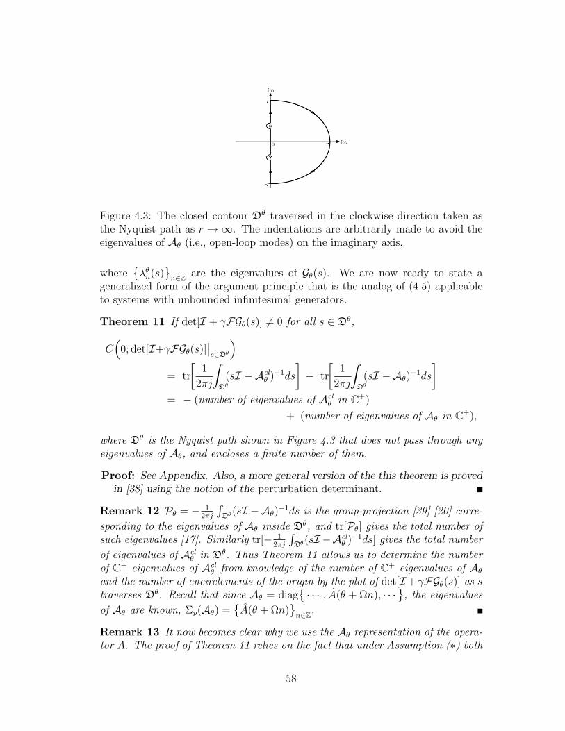
Figure 4.3: The closed contour D✓ traversed in the clockwise direction taken asthe Nyquist path as r ! 1. The indentations are arbitrarily made to avoid theeigenvalues of A
✓
(i.e., open-loop modes) on the imaginary axis.
where�
�✓
n
(s)
n2Z are the eigenvalues of G✓
(s). We are now ready to state ageneralized form of the argument principle that is the analog of (4.5) applicableto systems with unbounded infinitesimal generators.
Theorem 11 If det[I + �FG✓
(s)] 6= 0 for all s 2 D✓,
C⇣
0; det[I+�FG✓
(s)]�
�
s2D✓
⌘
= tr
1
2⇡j
Z
D✓
(sI �Acl
✓
)�1ds
�
� tr
1
2⇡j
Z
D✓
(sI �A✓
)�1ds
�
= � (number of eigenvalues of Acl
✓
in C+)
+ (number of eigenvalues of A✓
in C+),
where D✓ is the Nyquist path shown in Figure 4.3 that does not pass through anyeigenvalues of A
✓
, and encloses a finite number of them.
Proof: See Appendix. Also, a more general version of the this theorem is proved
in [38] using the notion of the perturbation determinant.
Remark 12 P✓
= � 12⇡j
R
D✓
(sI �A✓
)�1ds is the group-projection [39] [20] corre-
sponding to the eigenvalues of A✓
inside D✓, and tr[P✓
] gives the total number ofsuch eigenvalues [17]. Similarly tr[� 1
2⇡j
R
D✓
(sI�Acl
✓
)�1ds] gives the total number
of eigenvalues of Acl
✓
in D✓. Thus Theorem 11 allows us to determine the numberof C+ eigenvalues of Acl
✓
from knowledge of the number of C+ eigenvalues of A✓
and the number of encirclements of the origin by the plot of det[I+�FG✓
(s)] as straverses D✓. Recall that since A
✓
= diag� · · · , A(✓ + ⌦n), · · · , the eigenvalues
of A✓
are known, ⌃p
(A✓
) =�
A(✓ + ⌦n)
n2Z.
Remark 13 It now becomes clear why we use the A✓
representation of the opera-tor A. The proof of Theorem 11 relies on the fact that under Assumption (⇤) both
58
(sI�A✓
)�1 and (sI�Acl
✓
)�1 are compact operators, which means the infinitesimalgenerators A
✓
and Acl
✓
have discrete (pure point) spectrum for every value of ✓.This allows for the introduction of the group projections seen in Theorem 11 anddescribed in Remark 12. Such group projections can not be introduced for A andAcl since they have continuous spectrum in general.
Remark 14 Since A✓
has discrete spectrum, it has no finite accumulation pointsin the complex plane [17]. In particular, the eigenvalues of A
✓
can not converge toany finite point j!0 of the imaginary axis. Yet by itself this does not rule out thepossibility of the eigenvalues accumulating at ±j1. But Assumption (⇤⇤) guardsagainst this by requiring that A(k) be bounded away from the imaginary axis as|k| ! 1; see Remark 11. Thus the Nyquist path can be taken to run to infinityalong the imaginary axis without any technical di�culties.
As a direct consequence of Theorem 11 we have the following.
Theorem 12 Assume p✓
+ denotes the number of eigenvalues of A✓
inside C+.For D✓ taken as above, ⌃
p
(Acl
✓
) ⇢ C� i↵
(a) det[I + �FG✓
(s)] 6= 0, 8 s 2 D✓,
and
(b) C⇣
0; det[I + �FG✓
(s)]�
�
s2D✓
⌘
= p✓
+.
Finally, the closed-loop system Gcl is exponentially stable i↵ ⌃p
(Acl
✓
) ⇢ C� for all✓ 2 [0, ⌦].
4.4.2 The Eigenloci Method
The setback with the method described in the previous paragraph is that to show⌃p(Acl
✓
) ⇢ C�, Acl✓
= A✓
� B✓
�FC✓
, for di↵erent values of �, one has to plotdet[I + �FG
✓
(s)]�
�
s2D✓
for each �. Note that this includes having to calculatethe determinant of an infinite dimensional matrix. This motivates the followingeigenloci approach to Nyquist stability analysis, which is very similar to thatperformed in [8] for the case of time-periodic systems.
Let�
�✓
n
(s)
n2Z constitute the eigenvalues of FG✓
(s). Then
\ det[I + �FG✓
(s)] = \Y
n2Z
�
1 + ��✓
n
(s)�
. (4.6)
But recall from Lemma 10 that FG✓
(s) 2 B1(`2) for every s 2 ⇢(A✓
). This,in particular, means that FG
✓
(s) is a compact operator and thus its eigenvalues�✓
n
(s) accumulate at the origin as |n|!1 [32]. As a matter of fact one can makea much stronger statement.
59

Lemma 13 The eigenvalues �✓
n
(s), s 2 D✓, converge to the origin uniformly onD✓.
Proof: See Appendix.
Take the positive integer N✏
to be such that |�✓
n
(s)| < ✏, s 2 D✓, for all|n| > N
✏
. Let us rewrite (4.6) as
\ det[I + �FG✓
(s)] = \Y
|n|N
✏
�
1 + ��✓
n
(s)�
+ \Y
|n|>N
✏
�
1 + ��✓
n
(s)�
=X
|n|N
✏
\�
1 + ��✓
n
(s)�
+X
|n|>N
✏
\�
1 + ��✓
n
(s)�
. (4.7)
It is clear that if |�| < 1✏
then for |n| > N✏
we have |��✓
n
(s)| < 1, and 1 + ��✓
n
(s)can never circle the origin as s travels around D✓. Thus for |�| < 1
✏
the finalsum in (4.7) will not contribute to the encirclements of the origin, and hence welose nothing by considering only the first N
✏
eigenvalues. There still remain someminor technicalities.
First, let D✏
denote the disk |s| < ✏ in the complex plane. Then said truncationmay result in some eigenloci (parts of which reside inside D
✏
) not forming closedloops. But notice that these can be arbitrarily closed inside D
✏
, as this does nota↵ect the encirclements [8].
The second issue is that for some values of s 2 D✓, FG✓
(s) may have multipleeigenvalues, and hence there is ambiguity in how the eigenloci of the Nyquistdiagram should be indexed. But this poses no problem as far as counting theencirclements is concerned, and it is always possible to find such an indexing; fora detailed treatment see [40].
Let us denote by�
�✓
n
n2Z the indexed eigenloci that make up the generalized
Nyquist diagram. [To avoid confusion we stress the notation: �✓
n
(s) is the nth
eigenvalue of FG✓
(s) for a given point s 2 D✓, whereas �✓
n
is the nth eigenlocustraced out by �✓
n
(s) as s travels once around D✓.] From (4.7) and the abovediscussion it follows that
C⇣
0; det[I + �FG✓
(s)]�
�
s2D✓
⌘
=X
|n|N
✏
C⇣
� 1
�;�✓
n
⌘
which together with Theorem 12 gives the following.
Theorem 14 Assume p✓
+ denotes the number of eigenvalues of A✓
inside C+.For D✓ and N
✏
as defined previously, ⌃p
(Acl
✓
) ⇢ C� for |�| < 1✏
i↵
(a) �1
�/2 �
�✓
n
|n|N
✏
,
60

and
(b)P
|n|N
✏
C⇣
� 1
�;�✓
n
(s)⌘
= p✓
+.
Finally, the closed-loop system Gcl is exponentially stable i↵ ⌃p
(Acl
✓
) ⇢ C� for all✓ 2 [0, ⌦].
4.5 Numerical Implementation
4.5.1 Finite Truncations of System Operators
In the above development we showed that for a given ✏ > 0, the eigenloci that fallwithin the disk D
✏
= {s s.t. |s| < ✏} play no role in the Nyquist stability analysisand can be ignored as long as | 1
�
| > ✏.This suggests that one could truncate A
✓
, B✓
, C✓
, F first and then form atruncated version of FG
✓
(s) and compute its eigenloci, thus e↵ectively treating thestability problem as one for a family of (finite-dimentional) multivariable systemsdescribed by (4.3) parameterized by the variable ✓.
The complication here is that although a truncation removes the infinite num-ber of eigenloci that shrink to zero, it also a↵ects all other eigenloci no matterhow large the truncation is taken to be. Nevertheless, it can be shown that byincreasing the size of the truncation the eigenloci of FG
✓
(s) can be recovered toany accuracy.
As in Section 3.5 let ⇧ be the projection on the first 2N + 1 standard basiselements of `2, {e�N
, · · · , e0, · · · , eN
}, with the representation
⇧ = diagn
· · · , 0, 1, · · ·center#
, 1, · · · , 1| {z }
2N+1 times
, 0, · · ·o
.
Thus ⇧F⇧ is the (2N+1)⇥(2N+1) truncation of F , ⇧G✓
(s)⇧ = ⇧G✓
(s) = G✓
(s)⇧the (2N + 1)⇥ (2N + 1) truncation of G
✓
,5 and ⇧⇧ = ⇧. We have
Theorem 15 If ⇣ 2 ⇢�⇧F⇧G✓
(s)�
, s 2 D✓, and
kFG✓
(s)� ⇧F⇧G✓
(s)k k�⇣ � ⇧F⇧G✓
(s)��1k < 1, (4.8)
then ⇣ 2 ⇢�FG✓
(s)�
.
Proof: See Appendix.
5Recall that ⇧ commutes with G✓
(s) because the latter operator is diagonal.
61

Theorem 15 says that if a point ⇣ is not an eigenvalue of ⇧F⇧G✓
(s) then itwill not be an eigenvalue of FG
✓
(s) if (4.8) holds. But we need a stronger resultthat addresses the location of the eigenloci rather than the eigenvalues. Namelythat if ⇣ is does not belong to the eigenloci of the truncated system then it willnot belong to the eigenloci of the original system either. This is done in the nexttheorem.
Theorem 16 If ⇣ does not belong to the eigenloci of ⇧F⇧G✓
(s), s 2 D✓, and
maxs2D✓
kFG✓
(s)� ⇧F⇧G✓
(s)k maxs2D✓
k�⇣ � ⇧F⇧G✓
(s)��1k < 1, (4.9)
then ⇣ does not belong to the eigenloci of FG✓
(s), s 2 D✓.
Proof: The proof is simple and is omitted.
4.5.2 Regularity in the ✓ Parameter
In applying Theorems 12 and 14 one would hope for some kind of ‘regularity’with respect to the variable ✓. More concretely, in practice one would like toplot the eigenloci and check the Nyquist stability criterion for a finite number of✓
l
2 [0, ⌦), say ✓1, · · · , ✓L
, and be able to conclude stability for all ✓ 2 [0, ⌦) if the✓
l
are chosen close enough to each other.Indeed, it is possible to show that if det[I + �FG
✓
(s)] 6= 0 for all s 2 D✓ thendet[I + �FG
✓
(s)] is a continuous function of ✓ for all s 2 D✓. In other wordsall points of the plot det[I + �FG
✓
(s)]�
�
s2D✓
change continuously with ✓. Thisresult is easy to prove using techniques presented in [20] and we omit the details.Moreover, one can show that the following much stronger assertion.
Theorem 17 Let A(), B(), C() be analytic functions of on some strip
R = {⇣ s.t. � " Im(⇣) ", " > 0}
of the complex plane. Then the eigenloci�
�✓
n
n2Z of FG✓
(s) change continuouslywith ✓.
Proof: See Appendix.
4.6 An Illustrative Example
In this section we consider the example of a system governed by the spatiallyperiodic PDE
@t
(t, x) = @2x
(t, x) � � cos(x) (t, x) + (t, x), (4.10)
62

with � 2 C. Let us rewrite this system in the form of an open-loop spatiallyinvariant PDE described by
@t
(t, x) = @2x
(t, x) + (t, x) + u(t, x),
y(t, x) = (t, x),
placed in feedback with the spatially periodic function
�F (x) = � cos(x).
Now the problem is in the general from discussed in Section 4.3 with A = @2x
+ 1,B and C being the identity operator, and F (x) = cos(x) [thus ⌦ = 1]. SinceA(k) = �k2 + 1, k 2 R, Assumptions (⇤) is satisfied. Also, since ⌃(A) = (�1, 1]then Assumption (⇤⇤) is satisfied. Finally, from from A() = �2 +1 and B() =C() = 1 it is clear that these symbols are analytic on the entire complex planeand thus the conditions of Theorem 17 are satisfied.
The representation of the system in the frequency domain is @t
✓
(t) = (A✓
��F)
✓
(t), where A✓
= diag{· · · ,�(✓+n)2+1, · · · } for every ✓ 2 [0, 1) and F hasthe form shown in Example 1 of Section 2.5. Notice that the open-loop systemis unstable; for example at ✓ = 0, A
✓
has an eigenvalue at � = 1. Next wedemonstrate that by plotting the eigenloci one can read o↵ from this plot thestability of the closed-loop system for any value of � 2 C.
Recall that to test the stability of the closed-loop system, one has to apply theNyquist criterion for every ✓ 2 [0, 1). But since the conditions of Theorem 17 aresatisfied we need only carry out the Nyquist analysis for a finite number of ✓. Wetake Nyquist paths D✓ of the form shown in Figure 4.4(a) with r = 20. For every✓ the indentation in D✓ is chosen appropriately so as to avoid the eigenvalues ofA
✓
at the origin. Let us take a look at the Nyquist plots for two particular valuesof ✓:
✓ = 0 : � = 0, 0, 1 are the eigenvalues of A0 inside D0, hence p0+ = 3, and we
need three counter-clockwise encirclements of �1/� to achieve closed-loop stabil-ity. As can be seen in Figure 4.4(b) and its blown-up version (c), one possiblechoice would be to take �1/� to be purely imaginary and �0.2j �1/� 0.2j.Clearly such �1/� is encircled three times by the eigenloci.
✓ = 0.5 : � = 0.75, 0.75 are the eigenvalues of A0.5 inside D0.5, hence p0.5+ = 2,
and we need two counter-clockwise encirclements of �1/� to achieve closed-loopstability. Again, from Figure 4.4(d), if �1/� is taken to be purely imaginary and�0.2j �1/� 0.2j, then �1/� is encircled twice by the eigenloci.
We do not draw the Nyquist plots for other values of ✓ but it can be shown that�0.2j �1/� 0.2j stabilizes the closed-loop system for all values of ✓ 2 [0, 1)and thus stabilizes the original PDE (4.10).
63
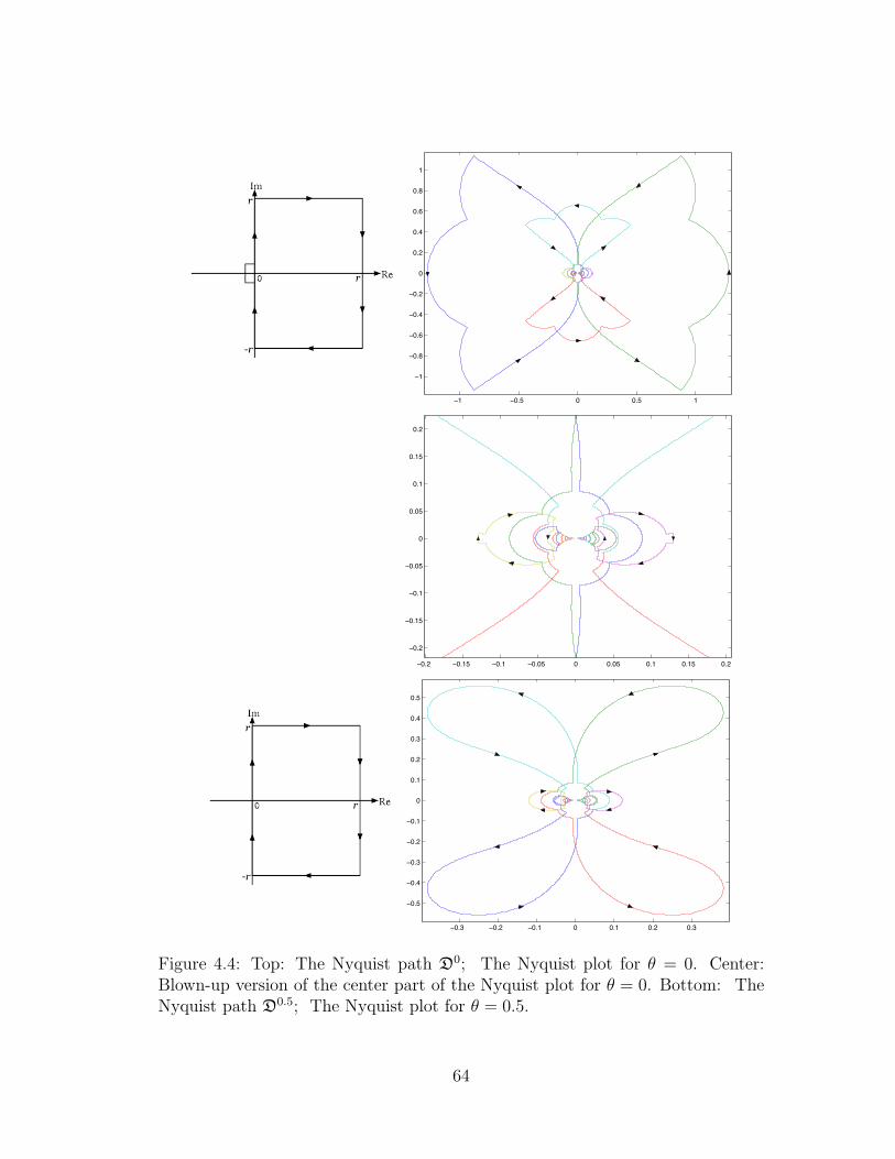
!1 !0.5 0 0.5 1
!1
!0.8
!0.6
!0.4
!0.2
0
0.2
0.4
0.6
0.8
1
!0.2 !0.15 !0.1 !0.05 0 0.05 0.1 0.15 0.2
!0.2
!0.15
!0.1
!0.05
0
0.05
0.1
0.15
0.2
!0.3 !0.2 !0.1 0 0.1 0.2 0.3
!0.5
!0.4
!0.3
!0.2
!0.1
0
0.1
0.2
0.3
0.4
0.5
Figure 4.4: Top: The Nyquist path D0; The Nyquist plot for ✓ = 0. Center:Blown-up version of the center part of the Nyquist plot for ✓ = 0. Bottom: TheNyquist path D0.5; The Nyquist plot for ✓ = 0.5.
64

4.7 Appendix to Chapter 4
Proof of Lemma 10
Since s 2 ⇢(A✓
), then s 6= A(✓+⌦n) for any n 2 Z, which means that all elementsof the diagonal operator (sI�A
✓
)�1 are finite. Let %n
�
(sI�A✓
)�1�
, n = 1, 2, · · · ,be a reordering of these diagonal elements such that |%1
�
(sI�A✓
)�1�| � |%2
�
(sI�A
✓
)�1�| � · · · � 0. Then �
n
�
(sI �A✓
)�1�
= |%n
�
(sI �A✓
)�1�|, where �
n
denotesthe nth singular value. But from Assumption (⇤) it follows that
P1n=1 �n
�
(sI �A
✓
)�1�
< 1. Hence (sI �A✓
)�1 2 B1(`2). But since B, C, and F are boundedoperators, so are B
✓
, C✓
, and F . Thus G✓
(s) 2 B1(`2) and FG✓
(s) 2 B1(`2) [20].
Proof of Theorem 11
To prove Theorem 11 we need the following lemma.
Lemma 18 For s 2 ⇢(A✓
), det[I + �FG✓
(s)] is analytic in both � and s.
Proof: For s 2 ⇢(A✓
), �FG✓
(s) 2 B1(`2) by Lemma 10. Also �FG✓
(s) =�FC
✓
(sI �A✓
)�1B✓
is clearly analytic in both � and s for s 2 ⇢(A✓
). Then it
follows from [20, p163] that det[I + �FG✓
(s)] too is analytic in both � and sfor s 2 ⇢(A
✓
).
Proof of Theorem 11: Consider any point s in D✓. Since D✓ does not passthrough any eigenvalues of A
✓
, s 2 ⇢(A✓
) and thus �FC✓
(sI �A✓
)�1B✓
2 B1(`2)
from Lemma 10. Then from [37],�I + �FC
✓
(sI �A✓
)�1B✓
��1exists and belongs
to B(`2) i↵ det[I + �FC✓
(sI �A✓
)�1B✓
] 6= 0, which is satisfied by assumption.
Applying the matrix inversion lemma to�I+�FC
✓
(sI�A✓
)�1B✓
��1, we conclude
that s 2 ⇢(Acl✓
) and (sI �Acl✓
)�1 = (sI �A✓
+ B✓
�FC✓
)�1 2 B(`2).Now since (sI �Acl
✓
)�1, B✓
, C✓
, and F all belong to B(`2), and (sI �A✓
)�1 2B1(`2), we have (sI � Acl
✓
)�1B✓
�FC✓
(sI � A✓
)�1 2 B1(`2) [20]. Thus, from theidentity
(sI �Acl✓
)�1 � (sI �A✓
)�1 = � (sI �Acl✓
)�1B✓
�FC✓
(sI �A✓
)�1,
it follows that (sI �Acl✓
)�1 2 B1(`2). In particular (sI �A✓
)�1 and (sI �Acl✓
)�1
are both in B1(`2), which means thatA✓
andAcl✓
both have discrete spectrum [17]and in
1
2⇡j
Z
D✓
(sI �Acl✓
)�1ds � 1
2⇡j
Z
D✓
(sI �A✓
)�1ds
= � 1
2⇡j
Z
D✓
(sI �Acl✓
)�1B✓
�FC✓
(sI �A✓
)�1ds
65
each term on the left side is a finite-dimensional projection [20, p11, p15]. Takingthe trace of both sides and changing the order of integration and trace on theright 6 we have
trh 1
2⇡j
Z
D✓
(sI �Acl✓
)�1dsi
� trh 1
2⇡j
Z
D✓
(sI �A✓
)�1dsi
= � 1
2⇡j
Z
D✓
tr[(sI �Acl✓
)�1B✓
�FC✓
(sI �A✓
)�1]ds. (4.11)
From [17], the left side of (4.11) is equal to the number of eigenvalues of A✓
in C+
minus the number of eigenvalues of Acl✓
in C+.On the other hand, let the path C✓ be that traversed by det[I + �FG
✓
(s)] ass travels once around D✓. By Lemma 18, det[I + �FG
✓
(s)] is analytic in s, and ifdet[I + �FG
✓
(s)] 6= 0 on D✓ we have
C⇣
0; det[I + �FG✓
(s)]�
�
s2D✓
⌘
=1
2⇡j
Z
C✓
dz
z
=1
2⇡j
Z
D✓
d
ds
det[I + �FG✓
(s)]
det[I + �FG✓
(s)]ds. (4.12)
Using [20, p163] and the assumption det[I + �FG✓
(s)] 6= 0, s 2 D✓, we arrive at
d
ds
det[I + �FG✓
(s)]
det[I + �FG✓
(s)]= tr
h
�I + �FG✓
(s)��1 d
ds�FG
✓
(s)i
= � tr[(sI �Acl✓
)�1B✓
�FC✓
(sI �A✓
)�1].
This, together with (4.12) and (4.11) gives the required result.
Proof of Lemma 13
For s 2 D✓ ⇢ ⇢(A✓
), det[I + �FG✓
(s)] is analytic in both � and s by Lemma 18.The proof now proceeds exactly as in [8, p140] and is omitted.
Proof of Theorem 15
This is a direct consequence of Theorem 3.17, Chap IV of [17]. Using the notationof [17], for s 2 D✓ take T := ⇧F⇧G
✓
(s), A := FG✓
(s) � ⇧F⇧G✓
(s), and S :=T + A = FG
✓
(s). Since T and A are bounded operators then b = 0 and a =kFG
✓
(s)� ⇧F⇧G✓
(s)k, again using the notation of [17]. The theorem statementnow follows from (4.8) and [17, p214].
6Since (sI �Acl
✓
)�1B✓
�FC✓
(sI �A✓
)�1 2 B1
(`2), its trace is well-defined and finite.
66

Proof of Theorem 17
It is simple to show that if A() is an analytic function of on R, then it is ananalytic family in the sense of Kato on R; see [41, p14]. We now form the operatorA
#
= diag� · · · , A(# + ⌦n), · · · where # is a variable on an open strip ⇥ that
contains the real interval [0, ⌦). It is immediate that A#
too is an analytic familyin the sense of Kato on ⇥. [The existence of ⇥ is guaranteed by the existence ofR.] Let ⌥ := {(#, z) | # 2 ⇥, z 2 ⇢(A
#
)}. Then from [41, Thm XII.7] it followsthat (z�A
#
)�1 is an analytic (operator-valued) function of the the two variables# and z on ⌥. In particular, if B() and C() are analytic functions of on Rthen FG
#
(z) = FB#
(z �A#
)�1C#
is an analytic (operator-valued) function of thethe two variables # and z on ⌥. Let �✓(s) be an eigenvalue of multiplicity i of thebounded operator FG
✓
(s), ✓ 2 [0, ⌦) and s 2 D✓. Then for (#, z) near (✓, s) thereare exactly i eigenvalues of FG
#
(z) near �✓(s) [17, p107]. We now restrict # andz to vary only on [0, ⌦) and D✓, respectively, and we have that the eigenvalues ofFG
✓
(s) are continuous in both ✓ and s in the sense just described. Since D✓ is aclosed set then it follows that the eigenloci
�
�✓
n
n2Z change continuously with ✓.
4.8 Summary
We develop a generalized Nyquist stability criterion that is applicable to open-loopsystems with infinite-dimensional input-output spaces and unbounded infinitesi-mal generators. We use this to verify the stability of spatially periodic systems,and in particular, systems governed by PDEs with periodic coe�cients.
67

Part II
Perturbation Methods in theAnalysis of Spatially Periodic
Systems
68
Chapter 5
Perturbation Analysis of the H2
Norm of Spatially PeriodicSystems
God does not care about our mathematical di�culties. He integrates empiri-cally. A. Einstein
5.1 Introduction
In Chapter 3 we showed that the H2-norm of a spatially periodic system can befound by solving a family of operator-valued algebraic Lyapunov equations. Wealso gave conditions under which the norm can be approximated arbitrarily-well bysolving the algebraic Lyapunov equations for finite but large-enough truncationsof the system operators. But even such approximation schemes can be numericallyexpensive as the truncation size becomes increasingly large.
In this chapter we take an analytic perturbation approach to approximatingtheH2-norm. Section 5.2 describes the general perturbation setup, and Section 5.3contains the main results. We finish the chapter with many examples in Section5.4.
Notation: To avoid clutter, we henceforth drop the “ˆ” from the representationof frequency domain functions. For example, we use A0( · ) [instead of A0( · )] torepresent the Fourier symbol of the spatially invariant operator Ao.
69
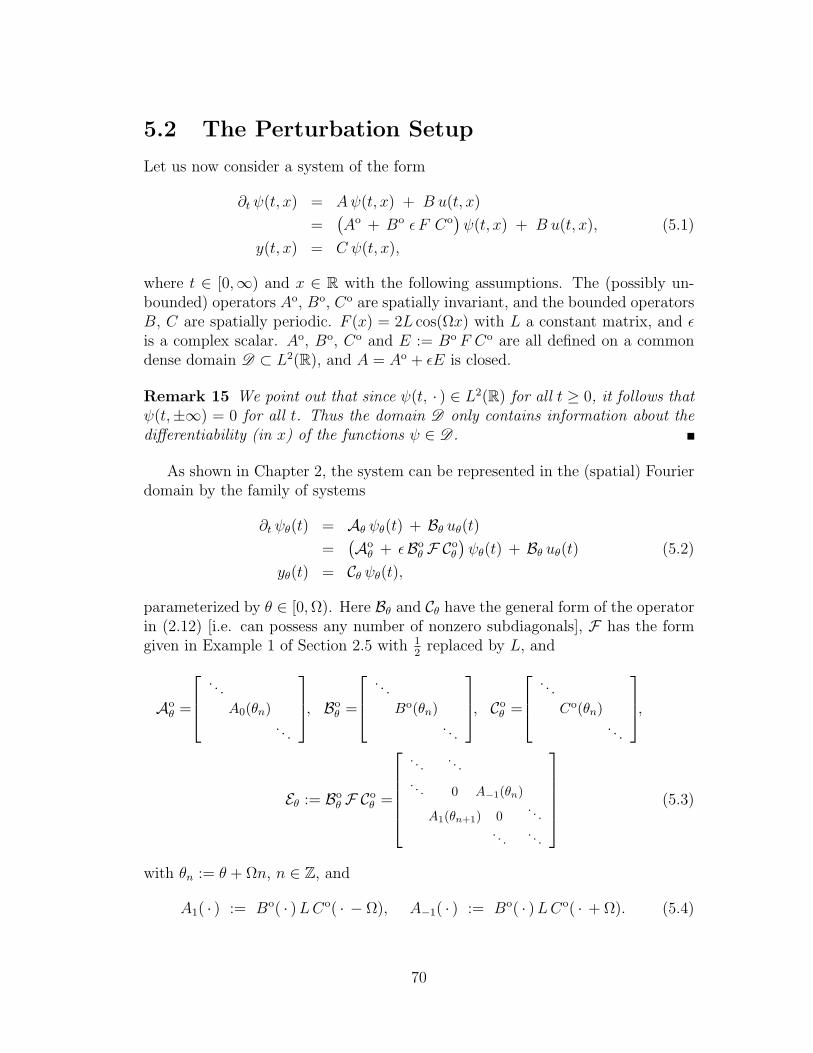
5.2 The Perturbation Setup
Let us now consider a system of the form
@t
(t, x) = A (t, x) + B u(t, x)
=�
Ao + Bo ✏F Co�
(t, x) + B u(t, x), (5.1)
y(t, x) = C (t, x),
where t 2 [0,1) and x 2 R with the following assumptions. The (possibly un-bounded) operators Ao, Bo, Co are spatially invariant, and the bounded operatorsB, C are spatially periodic. F (x) = 2L cos(⌦x) with L a constant matrix, and ✏is a complex scalar. Ao, Bo, Co and E := Bo F Co are all defined on a commondense domain D ⇢ L2(R), and A = Ao + ✏E is closed.
Remark 15 We point out that since (t, · ) 2 L2(R) for all t � 0, it follows that (t,±1) = 0 for all t. Thus the domain D only contains information about thedi↵erentiability (in x) of the functions 2 D .
As shown in Chapter 2, the system can be represented in the (spatial) Fourierdomain by the family of systems
@t
✓
(t) = A✓
✓
(t) + B✓
u✓
(t)
=�Ao
✓
+ ✏Bo✓
F Co✓
�
✓
(t) + B✓
u✓
(t) (5.2)
y✓
(t) = C✓
✓
(t),
parameterized by ✓ 2 [0, ⌦). Here B✓
and C✓
have the general form of the operatorin (2.12) [i.e. can possess any number of nonzero subdiagonals], F has the formgiven in Example 1 of Section 2.5 with 1
2replaced by L, and
Ao✓
=
2
6
4
.
.
.
A0(✓n
).
.
.
3
7
5
, Bo✓
=
2
6
4
.
.
.
B
o(✓n
).
.
.
3
7
5
, Co✓
=
2
6
4
.
.
.
C
o(✓n
).
.
.
3
7
5
,
E✓
:= Bo✓
F Co✓
=
2
6
6
6
6
4
.
.
.
.
.
.
.
.
. 0 A�1
(✓n
)
A
1
(✓n+1
) 0.
.
.
.
.
.
.
.
.
3
7
7
7
7
5
(5.3)
with ✓n
:= ✓ + ⌦n, n 2 Z, and
A1( · ) := Bo( · ) L Co( · � ⌦), A�1( · ) := Bo( · ) L Co( · + ⌦). (5.4)
70

Figure 5.1: Go has a spatially invariant infinitesimal generator Ao. The LFT ofGo and the spatially periodic multiplication operator ✏F yields a system whichhas a spatially periodic infinitesimal generator A.
We emphasize that the convention used in the representation of E✓
in (5.3) is thesame as that used in (2.12); for example the nth row of E
✓
is
{· · · , 0, A1(✓n
), 0, A�1(✓n
), 0, · · · }.
Remark 16 We note that taking F (x) to be a pure cosine is not restrictive. Theresults obtained here can be easily extended to problems where F (x) is any periodicfunction with absolutely convergent Fourier series coe�cients. The inclusion ofhigher harmonics of ⌦ in F (x), namely functions of frequency 2⌦, 3⌦, etc, wouldnot reveal new interesting phenomena and would only complicate the algebra.
Remark 17 Recall from Chapter 2 that the system (5.1) can be considered as theLFT (linear fractional transformation [27]) of a spatially periodic system Go withspatially invariant infinitesimal generator Ao,
Go =
2
6
4
Ao B Bo
C 0 0Co 0 0
3
7
5
and the (memoryless and bounded) spatially periodic pure multiplication operator✏F (x) = ✏ 2L cos(⌦x), see Figure 5.1.
5.3 Perturbation Analysis of the H2-Norm
In the rest of this chapter we assume that the system (5.1) is exponentially stableand has finite H2-norm for small enough values of ✏.
Now the di�culty in calculating the H2-norm using Theorem 3, is that unlessA
✓
, B✓
and C✓
are diagonal (i.e., G is a spatially invariant system), the operatorsP
✓
and Q✓
are “full”, meaning that they possess all of their (infinite number of)subdiagonals. This makes the computation of the H2-norm numerically intensive.Namely, one has to solve an infinite-dimensional algebraic Lyapunov equation to
71
find the operator P✓
(or Q✓
) for every value of ✓ 2 [0, ⌦). In this chapter we willsee how one can use analytic perturbation techniques to compute the H2-norm ina simple and numerically e�cient way, and without having to explicitly find thefull P
✓
and Q✓
operators. Such a perturbation analysis is very useful in predictinggeneral trends and extracting valuable information about the H2-norm.
Let us now consider the general setup of (5.1), with ✏ a small real scalar. Wealso assume that both Ao and A = Ao + ✏E define exponentially stable stronglycontinuous semigroups (also known as C0-semigroups) on L2(R) [3], and that Band C are spatially invariant operators. We are interested in the changes in theH2-norm of this system for small magnitudes of ✏ and di↵erent values of thefrequency ⌦.
Let us defineP
✓
(✏) := P(0)✓
+ ✏P(1)✓
+ ✏2P(2)✓
+ · · · ,
with P⇤✓
(✏) = P✓
(✏). Notice that this implies P(m)⇤✓
= P(m)✓
for all m = 0, 1, 2, · · · ,i.e., P(m)
✓
are selfadjoint operators for all m. The issue of convergence of the above
series is addressed in the Appendix to this chapter. Our aim is to find P(m)✓
bysolving the Lyapunov equation
A✓
(✏) P✓
(✏) + P✓
(✏)A⇤✓
(✏) ⌘ �B✓
B⇤✓
(5.5)
+(Ao
✓
+ ✏ E✓
) (P(0)✓
+ ✏P(1)✓
+ ✏2P(2)✓
+ · · · )+ (5.6)
(P(0)✓
+ ✏P(1)✓
+ ✏2P(2)✓
+ · · · ) (Ao✓
+ ✏ E✓
)⇤ ⌘ �B✓
B⇤✓
,
and compute the H2-norm of the system using Theorem 3
kGk2H2 =
1
2⇡
Z ⌦
0
trace[C✓
P✓
(✏) C⇤✓
] d✓.
It is easy to see from (5.6) that
Ao✓
P(0)✓
+ P(0)✓
Ao⇤✓
= �B✓
B⇤✓
, (5.7)
Ao✓
P(1)✓
+ P(1)✓
Ao⇤✓
= ��E✓
P(0)✓
+ P(0)✓
E⇤✓
�
, (5.8)
Ao✓
P(2)✓
+ P(2)✓
Ao⇤✓
= ��E✓
P(1)✓
+ P(1)✓
E⇤✓
�
, (5.9)...
Now since Ao✓
and B✓
B⇤✓
are diagonal in (5.7), so is P(0)✓
. In (5.8), the right handside operator has the structure of being nonzero only on the first upper and lowersubdiagonals, and hence P(1)
✓
inherits the same structure (since Ao✓
is diagonal).
In the same manner, one can show that P(2)✓
is only nonzero on the main diagonal
72

and the second upper and lower subdiagonals, and so on for other P(m)✓
. We have
P(0)✓
=
2
6
4
.
.
.
P0(✓n
).
.
.
3
7
5
, P(1)✓
=
2
6
6
6
6
4
.
.
.
.
.
.
.
.
. 0 P
⇤1
(✓n
)
P
1
(✓n
) 0.
.
.
.
.
.
.
.
.
3
7
7
7
7
5
,
P(2)✓
=
2
6
6
6
6
6
4
.
.
.
.
.
.
.
.
.
.
.
.
.
.
. 0 P
⇤2 (✓
n
).
.
. 0 Q0(✓n
) 0.
.
.
P2(✓n
) 0.
.
.
.
.
.
.
.
.
.
.
.
.
.
.
3
7
7
7
7
7
5
, . . .
where we have used the selfadjointness of these operators in representing theirsubdiagonals.
Remark 18 It is important to realize that, not only is P(m)✓
not a “full” operator,
it has at most m nonzero upper and lower subdiagonals. Also, all P(m)✓
for odd mhave zero diagonal and are thus trace-free operators.
Remark 19 Note that even though A✓
= Ao
✓
+ ✏ E✓
has only one nonzero subdiag-
onal [see (5.3)], P✓
(✏) = P(0)✓
+✏P(1)✓
+· · · possesses all of its subdiagonals. This isprecisely the reason why direct calculation of P
✓
in Theorem 3 is computationallydi�cult.
Now returning to (5.7)-(5.9), P(0)✓
, P(1)✓
and P(2)✓
are found by equating, elementby element, the bi-infinite matrices on both sides of these equations. For example,(5.7) leads to
A0(✓ + ⌦n) P0(✓ + ⌦n) + P0(✓ + ⌦n) A⇤0(✓ + ⌦n) = �B(✓ + ⌦n) B⇤(✓ + ⌦n)
for every n 2 Z, and ✓ 2 [0, ⌦). But notice that as n assumes values over allintegers and ✓ changes in [0, ⌦), k = ✓ + ⌦n takes all real values, and one canrewrite the above equation as
A0(k) P0(k) + P0(k) A⇤0(k) = �B(k) B⇤(k),
73

for all k 2 R. Applying the same procedure to (5.8)-(5.9), one arrives at
A0(k) P0(k) + P0(k) A⇤0(k) = �B(k) B⇤(k), (5.10)
A0(k) P1(k) + P1(k) A⇤0(k � ⌦) = �
⇣
A1(k) P0(k � ⌦) + P0(k) A⇤�1(k � ⌦)
⌘
,
(5.11)
A0(k) Q0(k) + Q0(k) A⇤0(k) = �
⇣
A1(k) P ⇤1 (k) + P1(k) A⇤
1(k)
+ A�1(k) P1(k + ⌦) + P ⇤1 (k + ⌦) A⇤
�1(k)⌘
,
(5.12)and so on for all nonzero diagonals of P(m)
✓
, m = 3, 4, · · · .Remark 20 Notice that from the above equations, one first finds P0( · ) from(5.10), then P1( · ) from (5.11), and so on. In other words, computing the subdiag-onals of P
✓
becomes “decoupled” in one direction. This decoupling would not havebeen possible had we not employed a perturbation approach and had attempted tosolve (5.5) directly.
Returning to the calculation of the H2-norm, let us first separate the diagonal
part of P(2)✓
by rewriting it as P(2)✓
= P(2)
✓
+ eP(2)✓
, where
P(2)
✓
:=
2
6
4
.
.
.
Q0(✓n
).
.
.
3
7
5
,
and eP(2)✓
contains the rest of P(2)✓
. Clearly trace[C✓
eP(2)✓
C⇤✓
] = 0. Also, recall that
trace[C✓
P(2m+1)✓
C⇤✓
] = 0, m = 0, 1, 2, · · · . (5.13)
Now one can write the following
kGk2H2 =
1
2⇡
Z ⌦
0
trace[C✓
P✓
(✏) C⇤✓
] d✓
=1
2⇡
Z ⌦
0
trace[C✓
P(0)✓
C⇤✓
+ ✏2 C✓
P(2)✓
C⇤✓
] d✓ + O(✏4)
=1
2⇡
Z ⌦
0
trace[C✓
P(0)✓
C⇤✓
+ ✏2 C✓
P(2)
✓
C⇤✓
] d✓ + O(✏4),
where the absence of odd powers of ✏ is due to (5.13), and the last equation follows
from the fact that trace[C✓
eP(2)✓
C⇤✓
] = 0. Next, using the unitaryness of the lifting
74

transform we haveZ ⌦
0
trace[C✓
P(0)✓
C⇤✓
] d✓ =
Z 1
�1trace[C(k) P0(k) C⇤(k)] dk,
Z ⌦
0
trace[C✓
P(2)
✓
C⇤✓
] d✓ =
Z 1
�1trace[C(k) Q0(k) C⇤(k)] dk,
and we arrive at the final result
kGk2H2 =
1
2⇡
Z 1
�1trace[C(k)P0(k)C⇤(k) + ✏2 C(k)Q0(k)C⇤(k)] dk + O(✏4). (5.14)
Remark 21 Let us stress again the important advantage of the above perturba-tion analysis in comparison to the method of Theorem 3. In the direct methodof computing the H2-norm proposed in Theorem 3, one has to solve a family ofinfinite-dimensional (operator) algebraic Lyapunov equations, whereas the pertur-bation method reduces the H2-norm computation to that of solving a family offinite-dimensional (matrix) Lyapunov/Sylvester equations (5.10)-(5.12).
In summary, we have the following.Main Result of Perturbation Analysis of H2-Norm Consider the expo-
nentially stable spatially periodic LTI system G, with spatial period X = 2⇡/⌦and state-space realization (5.1). Then for small values of |✏| the H2-norm ofthe system (5.1) can be computed from (5.14), where P0( · ) and Q0( · ) are solu-tions of the family of finite-dimensional Lyapunov/Sylvester equations describedby (5.10)-(5.12).
5.4 Examples
As an application of the perturbation results of the previous section, we first in-vestigate the occurrence of ‘parametric resonance’ for a class of spatially periodicsystems. Parametric resonance occurs when a specific frequency ⌦res of the peri-odic perturbation resonates with some ‘natural frequency’ { of the unperturbedsystem, leading to a local (in ⌦) change in system behavior [7]. In the systems weconsider in this section, this change in behavior is captured by the value of theH2-norm.
Example 4 Let us consider the periodic PDE
@t
= �(@2x
+ {2)2 � c + ✏ cos(⌦x) + u
y = , (5.15)
75

Figure 5.2: Above: Plot of P0( · ). Below: Plot of P0( · � ⌦) and P0( · + ⌦)(dashed).
with 0 6= { 2 R and c > 0. Comparing (5.15) and (5.1) we have
A0(k) = �(k2�{2)2�c, Bo(k) = 1, Co(k) = 1, B(k) = 1, C(k) = 1, L =1
2.
For this system, the functions P0(k) and Q0(k) of the previous section simplify to1
P0(k) =�1
2A0(k), (5.16)
Q0(k) =1
�
A0(k)�2
⇣ �1
2A0(k � ⌦)+
�1
2A0(k + ⌦)
⌘
(5.17)
= 4�
P0(k)�2�
P0(k � ⌦) + P0(k + ⌦)�
,
and it is our aim to find the H2-norm
kGk2H2 =
1
2⇡
Z 1
�1
�
P0(k) + ✏2 Q0(k)�
dk + O(✏4), (5.18)
for di↵erent values of the parameter ⌦ > 0. More specifically, we are interestedin the values of ⌦ for which the H2-norm is maximized.
From (5.16), P0(k) = 12
1(k2�{2)2+c
. The first plot of Figure 5.2 shows P0( · ),while the second shows P0( · � ⌦) and P0( · + ⌦) (dashed), for a given value of⌦ 6= 0. As ⌦ is increased, P0( · � ⌦) slides to the right and P0( · + ⌦) to theleft. From (5.17) it is clear that to find Q0( · ) for any ⌦, one would sum thetwo functions in the second plot and multiply the result by the square of the firstplot. The interesting question now is, for what value(s) of ⌦ 2 (0,1) would theH2-norm in (5.18) be maximized.
One can easily see that as ⌦ ! 0, the peaks of P0( · �⌦) and P0( · +⌦) merge
1To find Q
0
(k) one needs to first find P
1
(k), but we have omitted the details for brevity.
76

ï2 ï1.5 ï1 ï0.5 0 0.5 1 1.5 20
2
4
6
P 0(k)
k
0 0.5 1 1.5 2 2.5 3 3.5 40
50
100
1
0 ï'
' Q
0(k) d
k
0
0.05
0.1
0.15
0.2 00.5
11.5
22.5
3
0.75
0.8
0.85
0.9
0.95
1
1.05
1.1
1.15
!
"
H2 N
orm
Figure 5.3: Left: Plots of Example 4 for { = 1 and c = 0.1. Notice that the firstgraph is plotted against k and the second against ⌦. Right: The plot of H2-normof the same example, but calculated by taking large truncations of the A
✓
, B✓
, C✓
matrices and using Theorem 3.
toward those of�
P0( · )�2
, thusR1�1 Q0(k) dk grows and hence kGk2
H2 grows.2 Thisis not surprizing; as ⌦ ! 0, the perturbation is tending toward a constant functionF (x) = cos(⌦x) ! 1. This results in shifting the whole spectrum of Ao towardthe right-half of the complex plane, thus increasing the H2-norm of the perturbedsystem.
But we are more interested in frequencies ⌦ � 0 that lead to a local (in ⌦)increase in the H2-norm. Now notice that a di↵erent alignment of the peaks canalso occur, which leads to another local maximum of the H2-norm as a functionof ⌦. This happens when the peak of P0( · � ⌦) at k = �{ + ⌦ becomes aligned
with the peak of�
P0( · )�2
at k = {, and, simultaneously, the peak of P0( · + ⌦)
at k = { � ⌦ becomes aligned with the peak of�
P0( · )�2
at k = �{. Clearly thisoccurs when
�{ + ⌦res
= { =) ⌦res
= 2 {.
This result agrees exactly with that obtained in [26], where in the analysis of thesame problem it is shown that the part of the spectrum of A closest to the imaginaryaxis ‘resonates’ with perturbations whose frequency satisfies the relation ⌦ = 2 {.
Consider (5.15) with { = 1 and c = 0.1. For this systemR1�1 P0(k) dk ⇡ 4.74.
Figure 5.3 (left) shows the graphs of P0( · ) (plotted against k) andR1�1 Q0(k) dk
(plotted against ⌦). The peak at ⌦ = 2 in the lower plot verifies the result ⌦res
=2 { obtained above.
Figure 5.3 (right) shows the H2-norm of this system computed by taking large
2Remember that P
0
(k) is independent of ⌦, and thusR1�1 P
0
(k) dk remains constant fordi↵erent ⌦.
77

!2 !1.5 !1 !0.5 0 0.5 1 1.5 20
2
4
6
P0(k
)
k
0 0.5 1 1.5 2 2.5 3 3.5 4!10
!5
0
!
" !#
# Q
0(k
) dk
Figure 5.4: The plot of Example 4 with { = 1 and c = 0.1 and a purely imaginaryperturbation.
enough truncations of the A✓
, B✓
, C✓
matrices and then applying Theorem 3. Thefigure shows that the trends were indeed correctly predicted by the perturbationanalysis; the peaks at ⌦ = 0, 2 correspond to those of
R1�1 Q0(k) dk.
Now consider (5.15) with { = 1 and c = 0.1, but with ✏ replaced by ✏j; thiswould correspond to L = j/2 in that example. Obviously the unperturbed systemremains the same as before and hence
R1�1 P0(k) dk ⇡ 4.74. Figure 5.3 shows the
graph ofR1�1 Q0(k) dk, which demonstrates that for this system the purely imagi-
nary perturbation reduces the H2-norm at all frequencies. We address the physicalinterpretation of such a perturbation in the Appendix.
We continue with more examples to demonstrate that by appropriately choos-ing the frequency of the perturbation, one can decrease or (as in the previousexample) increase the H2-norm of the unperturbed system.
Example 5 Let us consider the periodic PDE [34]
@t
= �(@2x
+ {2)2 � c + ✏ cos(⌦x) @x
+ u
y = . (5.19)
Comparing (5.19) and (5.1) we have
A0(k) = �(k2�{2)2�c, Bo(k) = 1, Co(k) = jk, B(k) = 1, C(k) = 1, L =1
2.
The di↵erence between this system and (5.15) is that here Co is a spatial derivative.The plot of Figure 5.5 demonstrates
R1�1 Q0(k) dk for { = 1 and c = 0.1. Notice
that the peak at ⌦res
= 2 remains the same as in Figure 5.3, but we now havea decrease at small frequencies. This is due to the derivative operator Co = @
x
.Finally, notice the agreement of the perturbation analysis here with the (non-perturbation) calculations for the same system in the First Example of Section3.6. Our perturbation methods correctly predict the increase at ⌦ = 2 and thedecrease around ⌦ ⇡ 0.4 of the H2-norm.
78

!2 !1.5 !1 !0.5 0 0.5 1 1.5 20
2
4
6
P0(k
)
k
0 0.5 1 1.5 2 2.5 3 3.5 4!20
0
20
40
60
!
" !#
# Q
0(k
) dk
Figure 5.5: Plot of Example 5 for { = 1 and c = 0.1.
ï4 ï3 ï2 ï1 0 1 2 3 40
2
4
6
8
k
trace
(CP 0(k
)C*)
0 1 2 3 4 5 6ï50
0
50
100
150
1
0 ï'
' tr
ace(
CQ0C*
) dk
Figure 5.6: Graphs of Example 6 for R = 6 and c = 1.
Example 6 The following system is motivated by channel flow problems
A0(k) =� 1
R
(k2 + c) 0jk � 1
R
(k2 + c)
�
Bo(k) =⇥
1 00 1
⇤
, Co(k) =⇥
1 00 1
⇤
, B(k) =⇥
1 00 0
⇤
, C(k) =⇥
0 00 1
⇤
, L =1
2
⇥
0 �11 0
⇤
.
We perform numerical calculations for R = 6, c = 1. We haveZ 1
�1trace[C(k)P0(k)C⇤(k)] dk ⇡ 20.72.
Figure 5.6 shows that the H2-norm can be decreased by the the application ofperiodic perturbations with frequency ⌦ ⇡ 0.7. It is interseting that if one uses thelocations of the peaks in the first plot of Figure 5.6 to find { = 0.75, then from thepeak at ⌦
res
= 1.6 in the second plot it seems that the relationship ⌦res
⇡ 2{ = 1.5still holds with an acceptable error even for this non-scalar example.
79

5.5 Appendix to Chapter 5
Convergence of the Perturbation Series
For the series expansion
P✓
(✏) = P(0)✓
+ ✏P(1)✓
+ ✏2P(2)✓
+ · · ·
to be valid, we must show that all elements of P✓
(✏) converge for ✏ contained insome small enough domain. Let us assume that Bo and Co are bounded operators,and (without loss of generality) that sup
k2R kB(k)k = 1. Assume keA0(k)tk M
k
e%
k
t, and define
M := supk2R
Mk
< 1, � ↵0 := supk2R
%k
< 0,
↵1 := max{supk2R
kA1(k)k, supk2R
kA�1(k)k}.
Notice that the finiteness of M and the negativity of �↵0 follow from the expo-nential stability of the unperturbed system. Now from (5.10) we have
P0(k) =
Z 1
0
eA0(k)tB(k)B⇤(k) eA
⇤0(k)t dt,
and therefore
supk2R
kP0(k)k M2
2↵0
=: µ.
Similarly, from (5.11) we have
P1(k) =
Z 1
0
eA0(k)t�
A1(k)P0(k � ⌦) + P0(k)A⇤�1(k � ⌦)
�
eA
⇤0(k�⌦)t dt,
and therefore
supk2R
kP1(k)k M2
2↵0
(2↵1µ) µ(4↵1µ) = 4↵1µ2.
From (5.12) we have
Q0(k) =
Z 1
0
eA0(k)t�
A1(k)P ⇤1 (k) + · · ·+ P ⇤
1 (k + ⌦)A⇤�1(k)
�
eA
⇤0(k)t dt,
and therefore
supk2R
kQ0(k)k M2
2↵0
(4↵1(4↵1µ2)) µ(4↵1)
2µ2 = (4↵1)2µ3.
80

In fact it is possible to show that any element of P(m)✓
is bounded by
(4↵1)mµ(m+1).
Thus for all |✏| < 4↵1µ = 2M2↵1/↵0 the series expansion of P✓
(✏) converges.
5.6 Summary
We use perturbation analysis to find a computationally e�cient way of revealingtrends in the H2-norm of spatially periodic systems. We show that the basicfrequency of the periodic perturbation can be chosen so as to increase (by in-ducing parametric resonance) or decrease the H2-norm. We demonstrate thatfor certain scalar systems, the value of the spatial period that achieves the de-sired increase/decrease of the H2-norm can be characterized exactly, based on thedescription of the nominal system.
81

Chapter 6
Stability and the SpectrumDetermined Growth Conditionfor Spatially Periodic Systems
Everything should be made as simple as possible, but not simpler. A. Einstein
6.1 Introduction
As mentioned briefly in Section 4.2, in the literature on semigroups there existexamples in which ⌃(A) lies entirely inside C� but keAtk does not decay expone-tially [14] [15]. In such cases it is said that the semigroup does not satisfy thespectrum-determined growth condition [16]. The determining factor in the ex-amples presented in [14] and [15] can be interpreted as the accumulation of theeigenvalues of A
✓
around ±j1 in the form of Jordan blocks of ever-increasingsize (i.e. as the eigenvalues tend to ±j1 their algebraic multiplicity increaseswhile their geometric multiplicity stays finite). But such cases are ruled out whenone deals with holomorphic semigroups, which is the reason we consider thesesemigroups in this chapter.
Our ultimate aim in this chapter is to verify exponential stability. In Section6.3 we describe a class of infinitesimal generators A for which ⌃(A) ⇢ C� yieldsexponential stability. Section 6.4 then gives conditions under which our spatiallyperiodic infinitesimal generators belong to this class. And in Section 6.5 we findsu�cient conditions which guarantee ⌃(A) ⇢ C�.
The setup is the same as that in Section 5.2 with ✏ a small complex scalar.In addition, assume that A0(k) 2 Cq⇥q is diagonalizable for every k 2 R. As inthe previous chapter, to avoid clutter we drop the “ˆ” from the representation offrequency domain functions.
82
6.2 Spectrum of Spatially Invariant Operators
Recall that for a general spatially periodic operator A we have
⌃(A) =[
✓2[0,⌦)
⌃(A✓
). (6.1)
In the case where A is spatially invariant [and thus A✓
= diag {· · · , A0(✓n
), · · · }],(6.1) further simplifies to
⌃(A) =[
k2R⌃p(A0(k)). (6.2)
Example 7 Let A = �(@2x
+ {2)2 with domain
D = {� 2 L2(R) | �,d�
dx,d2�
dx2,d3�
dx3absolutely continuous,
d4�
dx42 L2(R)}. (6.3)
An integration by parts shows that A is a self-adjoint operator and thus closed.A0(k) = �(k2 � {2)2 is the Fourier symbol of A, see Figure 6.1 (top). SinceA0( · ) is scalar, ⌃
p
�
A0(k)�
= A0(k) for every k. It is easy to see that A0( · )takes every real negative value and thus from (6.2) A has continuous spectrum⌃(A) = (�1, 0 ], see Figure 6.1 (center).
Remark 22 When A is spatially invariant, a helpful way to think about ⌃(A) interms of the symbol A0( · ) of A is suggested by the previous example. First plot⌃
p
(A0( · )) in the ‘complex-plane⇥ spatial-frequency’ space, as in Figure 6.1 (top)of Example 7. Then the orthogonal projection onto the complex plane of this plotwould give ⌃(A), as in Figure 6.1 (center). This can be considered as a geometricinterpretation of (6.2). In Example 7, since A0( · ) is real scalar and takes onlynegative values, this projection yields only the negative real axis. But in general ifA0( · ) 2 Cq⇥q, this projection would lead to q curves in the complex plane. Noticealso that in this setting, ⌃(A
✓
) is the projection onto the complex plane of samplesof ⌃
p
(A0( · )) taken at k = ✓n
= ✓ + ⌦n, n 2 Z, in the ‘complex-plane⇥ spatial-frequency’ space. This can be considered as a geometric interpretation of (6.1).Figure 6.1 (bottom) shows these samples in the ‘complex-plane⇥ spatial-frequency’space for a scalar A.
6.3 Sectorial Operators
We next introduce a special subclass of holomorphic (or analytic) semigroups.The reader is referred to [17–19] for a detailed discussion. Suppose A is densely
83

Figure 6.1: Top: Representation of the symbol A0( · ) of Example 7 in ‘complex-plane ⇥ spatial-frequency’ space. Center: ⌃(A) in the complex plane. Bottom:For spatially invariant A, the (diagonal) elements of A
✓
are samples of the Fouriersymbol A0( · ).
84
defined, ⇢(A) contains a sector of the complex plane | arg(z�↵) | ⇡
2+ �, � > 0,
↵ 2 R, and there exists some M > 0 such that
k(zI � A)�1k M
|z � ↵| for | arg(z � ↵) | ⇡
2+ �. (6.4)
Then A generates a holomorphic semigroup and we write A 2 H (�,↵, M) [19][17]. We say that A is sectorial if A belongs to some H (�,↵, M).
Theorem 19 Assume that A is sectorial. Then if ⌃(A) ⇢ C�, A generates anexponentially stable semigroup.
Proof: If A is sectorial it defines a holomorphic semigroup, and thus eAt
is di↵er-
entiable for t > 0 [18]. Then [16] shows that this is su�cient for the spectrum-
determined growth condition to hold. Since ⌃(A) ⇢ C�and A is sectorial, then
⌃(A) is bounded away from the imaginary axis. Let !�
:= supz2⌃(A) Re(z).
Then !�
< 0 and A generates an exponentially stable semigroup.
6.4 Conditions for Infinitesimal Generator to beSectorial
To find conditions under which A in (5.1) will define a holomorphic semigroup wehave to check the condition (6.4). Since the Fourier transform preserves norms,(6.4) is equivalent to checking k(zI � A)�1k M/|z � ↵| for z belonging to somesector of C. This involves finding the inverse of the operator zI � A and thencalculating its norm. Such a computation can be very di�cult since (zI�A)�1 hasthe form (2.9) [also depicted in Figure 2.2 (right)], i.e., it has an infinite numberof impulse sheets. On the other hand, finding k(zI � Ao)�1k is very easy, due tothe diagonal structure of Ao. Indeed k(zI � Ao)�1k = sup
k2R k(zI � A0(k))�1k.Thus to establish conditions for A to be sectorial, we again use perturbation
theory. We first find conditions under which Ao is sectorial. We then show thatA = Ao + ✏E remains sectorial if E is ‘weaker’ than Ao in a certain sense we willdescribe, and if ✏ is small enough.
In the next theorem we present a condition for a spatially invariant Ao withFourier symbol A0( · ) to be sectorial.
Theorem 20 Let A0(k) be diagonalizable for every k 2 R, and let U(k) be thetransformation that diagonalizes A0(k), i.e., A0(k) = U(k) ⇤(k) U�1(k) with ⇤(k)diagonal. Let (k) := kU(k)k kU�1(k)k denote the condition number of U(k). Ifsup
k2R (k) <1, and for every k 2 R the resolvent set ⇢(A0(k)) contains a sectorof the complex plane | arg(z�↵) | < ⇡
2+� with � > 0 and ↵ 2 R both independent
of k, then Ao is sectorial.
85
Proof: See Appendix.
This theorem has a particularly simple interpretation when A0( · ) is scalar. Inthis case (k) = 1 for all k 2 R. Now since A0( · ) traces a curve in the complexplane, by Theorem 20 if this curve stays outside some sector | arg(z�↵) | ⇡
2+�,
� > 0, of the complex plane then Ao is sectorial.The following theorem is the main result of this section and uses the notion
of relative boundedness of one unbounded operator with respect to another un-bounded operator [17] to prove that A = Ao + ✏E is sectorial.
Theorem 21 Let Ao with domain D be a closed operator, and Ao 2H (�,↵, M).Let E = Bo F Co with domain D 0 � D be relatively bounded with respect to Ao
such thatkE k a k k + b kAo k, 2 D , (6.5)
with 0 a < 1 and 0 b |✏| < 1/(1 + M). Then A = Ao + ✏E is a closed andsectorial operator.
Proof: From (6.5) we have
k✏E k a |✏| k k + b |✏| kAo k
Then from [19, Thm 4.5.7] it follows that A = Ao + ✏E is sectorial for 0 b |✏| < 1/(1 + M). Also since M > 0, then b |✏| < 1 and [17, Thm IV.1.1] gives
that A is closed.
This theorem says that if Ao is sectorial and closed, then so is A = Ao + ✏Eif E is weaker than Ao in the sense of (6.5) and if |✏| is small enough. Noticethat at this point, condition (6.5) can not be reduced to a condition in termsof Fourier symbols (i.e. a condition that can be checked pointwise in k) as inTheorem 20. This is because E is not spatially invariant. But once the exactform of the operators Bo and Co is known, (6.5) can be simplified to a conditionon the symbols of Ao, Bo and Co. Let us clarify this statement with the aid of anexample.
Example 8 Consider the periodic PDE
@t
= �(@2x
+ {2)2 � c + ✏ @x
cos(⌦x) + u
y = ,
where 2 D , and D is defined as in (6.3). It is easy to see that Ao = �(@2x
+{2)2 � c is sectorial by Theorem 20 and closed by Example 7, Bo = @
x
, andCo = �(x) [the identity convolution operator]. By formal di↵erentiation we have
E = @x
cos(⌦x) = � ⌦ sin(⌦x) + cos(⌦x) @x
.
86

Using the triangle inequality and k sin(⌦x)k = k cos(⌦x)k = 1 we have
kE k |⌦| k k + k@x
k. (6.6)
Thus we have e↵ectively ‘commuted out’ the bounded spatially periodic componentof E, and are left with only spatially invariant operators on the right of (6.6).Hence, after applying a Fourier transfomation to the right side of (6.6), a su�cientcondition for (6.5) to hold is that
|⌦| + |k| a + b |(k2 � {2)2 + c|, k 2 R,
which can be shown to be satisfied for large enough a > |⌦| and b > 0. UsingTheorem 21, A is sectorial and closed for small enough |✏|.Remark 23 The above example makes clear the notion of E being ‘weaker’ thanAo that we mentioned at the beginning of this section. If in Example 8 we hadBo = @⌫
x
and Co = @µ
x
and ⌫+µ = 5, then E would contain a 5th order derivative,whereas the highest order of @
x
in Ao is 4. This would mean that (6.5) can not besatisfied for any choice of a and b.
6.5 Conditions for Infinitesimal Generator tohave Spectrum in C�
The final step in establishing exponential stability is to show that ⌃(A) ⇢ C�.Unfortunately it is in general very di�cult to find the spectrum of an infinite-dimensional operator. Thus we proceed as follows. We consider the (block) diag-onal operators Ao
✓
, ✓ 2 [0, ⌦). This allows us to extend Gersgorin-type methods(existing for finite-dimensional matrices) to find bounds on the location of ⌃(A
✓
),A
✓
= Ao✓
+ ✏ E✓
. In turn, we use this to find conditions under which ⌃(A✓
) ⇢ C�,and thus ⌃(A) ⇢ C�.
In locating the spectrum of a finite-dimensional matrix T 2 Cq⇥q, the theory ofGersgorin circles [42] provides us with a region of the complex plane that containsthe eigenvalues of T . This region is composed of the union of q disks, the centersof which are the diagonal elements of T , and their radii depend on the magnitudeof the o↵-diagonal elements [42]. This theory has also been extended to the caseof finite-dimensional block matrices (i.e., matrices whose elements are themselvesmatrices) in [43]. Next, we further extend this theory to include bi-infinite (block)matrices A
✓
.For the operator A = Ao + ✏E, take B
k
to be the set of complex numbers zthat satisfy
�min(zI � A0(k)) |✏| �kA�1(k)k+ kA1(k)k�, (6.7)
where �min(zI�A0(k)) denotes the smallest singular value of the matrix zI�A0(k).
87

Lemma 22 For every ✓ we have ⌃(A✓
) ✓ S✓
, where
S✓
=[
n2ZB
✓
n
.
Proof: See Appendix.
Example 9 Let us consider the periodic PDE [34]
@t
= �(@2x
+ {2)2 � c + ✏ cos(⌦x) @x
+ u
y = . (6.8)
where 2 D , and D defined as in (6.3). Comparing (6.8) and (5.1) we have
A0(k) = �(k2�{2)2�c, Bo(k) = 1, Co(k) = jk, B(k) = 1, C(k) = 1, L =1
2.
From (5.4), A1(k) = j
2(k�⌦), A�1(k) = j
2(k+⌦), and thus kA�1(k)k+kA1(k)k =
12(|k � ⌦|+ |k + ⌦|). Hence (6.7) leads to
�min
(zI�A0(k)) = |zI�A0(k)| |✏|2
(|k�⌦|+ |k+⌦|) =
⇢
⌦ |✏| |k| ⌦|k| |✏| |k| � ⌦
,
which means that the set S✓
is composed of the union of disks with centers atA0(✓n
) and radii |✏|2(|✓
n
� ⌦| + |✓n
+ ⌦|). This is nothing but an extension of theclassical Gersgorin disks to bi-infinite matrices. Figure 6.2 (top & center) showS
✓
in the complex-plane⇥ spatial-frequency space and in C respectively.1
Remark 24 The set
⌃"
(T ) := {z 2 C | �min
(zI � T ) "} (6.9)
= {z 2 C | k(zI � T )'k " for some k'k = 1}= {z 2 C | z 2 ⌃
p
(T + Z) for some kZk "}
is called the "-pseudospectrum of the matrix T [44]. Clearly ⌃"
0(T ) ✓ ⌃"
(T ) if"0 ", and ⌃
"
(T ) = ⌃p
(T ) for " = 0. The pseudospectrum is composed of smallsets around the eigenvalues of T . For instance if T has simple eigenvalues, thenfor small enough values of " the pseudospectrum consists of disjoint compact andconvex neighborhoods of each eigenvalue [45].
1We would like to point out that Figure 6.2 (top) is technically incorrect; once the spatiallyinvariant system is perturbed by a spatially periodic perturbation it is no longer spatially invari-ant and thus can not be represented by a Fourier symbol. Hence its spectrum can no longer bedemonstrated in the complex-plane⇥ spatial-frequency space. Figure 6.2 (center) demonstratesthe correct representation of the Gersgorin disks for A
✓
.
88

Figure 6.2: Top: The B✓
n
regions viewed in the ‘complex-plane ⇥ spatial-frequency’ space (the disks are parallel to the complex plane). Center: ⌃(A
✓
)is contained inside the union of the regions B
✓
n
. Bottom: The bold line shows⌃(Ao) and the dotted region contains ⌃(A), A = Ao + ✏E.
89

Remark 25 Comparing (6.9) and the definition of Bk
in (6.7), it is clear thatB
k
= ⌃"
(A0(k)) with " = |✏| �kA�1(k)k + kA1(k)k�. Thus for every k 2 R, (6.7)defines a closed region of C that includes the eigenvalues of A0(k).
We now employ Lemma 22 to determine whether ⌃(A) resides completelyinside C�, as needed to assess system stability. Take D
"
to be the closed diskof radius " and center at the origin, and B
k
to be the region described by (6.7).Define the sum of sets by U1 + U2 = {z | z = z1 + z2, z1 2 U1, z1 2 U1}. Also, forevery k 2 R let �max(k) represent the eigenvalue of A0(k) with the maximum realpart, and let (k) be defined as in Theorem 20.
Theorem 23 For every k, Bk
is contained inside ⌃p
(A0(k)) + Dr(k) with
r(k) = |✏| �kA�1(k)k+ kA1(k)k�(k).
In particular, if ⌃(Ao) ⇢ C� and
r(k) < |Re(�max
(k))|+ � (6.10)
for every k 2 R and some � < 0 independent of k, then ⌃(A) ⇢ C�.
Proof: See Appendix.
Example 10 Once again we use the scalar system of Example 9. (k) = 1 sinceA0(k) is scalar, |Re(�
max
(k))| = |(k2 � {2)2 + c|, and
kA�1(k)k+ kA1(k)k =1
2(|k � ⌦|+ |k + ⌦|).
Thus condition (6.10) becomes
|✏|2
(|k � ⌦|+ |k + ⌦|) < |(k2 � {2)2 + c|+ �.
If this condition is satisfied for some � < 0, the dotted region in Figure 6.2(bottom) will remain inside C� and thus ⌃(A) ⇢ C�.
6.6 Appendix to Chapter 6
Proof of Theorem 20
It is shown in [46] that a su�cient condition for Ao to be sectorial is that ⇢(Ao)contain some right half plane {z 2 C |Re(z) � µ}, and
kz(zI � Ao)�1k M for Re(z) � µ,
90
for some µ � 0 and M � 1.Now since A0(k) 2 Cq⇥q is diagonalizable for every k, there exists a matrix
U(k) such that A0(k) = U(k) ⇤(k) U�1(k) with ⇤(k) a diagonal matrix. Let�
i
(k), i = 1, · · · , q denote the diagonal elements of ⇤(k). Clearly these are alsothe eigenvalues of A0(k). Thus we have
kz(zI � Ao)�1k supk2R
⇣
kz(zI � A0(k))�1k⌘
supk2R
⇣
kU(k)k kU�1(k)k kz(zI � ⇤(k))�1k⌘
= supk2R
⇣
(k)|z|
dist[z, ⌃p(A0(k))]
⌘
max supk2R
⇣ |z|dist[z, ⌃p(A0(k))]
⌘
,
where max := supk2R (k).
Let us now choose the positive scalar M 0 = (1+max)M , M > 1, and considerfor a given k the region of the complex plane where
max|z|
dist[z, ⌃p(A0(k))]� M 0.
This region (which contains the eigenvalues �i
(k)) is contained inside the unionof the circles
max|z|
|z � �i
(k)| � M 0, i = 1, · · · , q,
which are themselves contained inside the larger circles
|z � �i
(k)| |�i
(k)|M
, i = 1, · · · , q. (6.11)
Notice that (6.11) describes circles whose radii increase like |�i
(k)|/M , M > 1, astheir centers �
i
(k) become distant from the origin. Clearly a su�cient conditionfor these circles to belong to some open half plane {z 2 C |Re(z) < µ} for allk 2 R and large enough M is that ⌃p(A0(k)), k 2 R, reside outside some sector| arg(z � ↵) | ⇡
2+ �, � > 0, of the complex plane.
Finally, if the circles (6.11) are contained in some open half plane {z 2C |Re(z) < µ} for all k 2 R, then for Re(z) � µ, z 2 ⇢(A0(k)) and we have
max supk2R
⇣ |z|dist[z, ⌃p(A0(k))]
⌘
M
and thus kz(zI � Ao)�1k M for Re(z) � µ.
91
Proof of Lemma 22
We use ⇧N
T ⇧N
to denote the (2N + 1) ⇥ (2N + 1) [block] truncation of anoperator T on `2, as defined in Section 3.5. We now form the finite-dimensionalmatrix ⇧
N
A✓
⇧N
�
�
⇧N
`
2 by restricting ⇧N
A✓
⇧N
to the finite-dimensional space
⇧N
`2. Clearly ⇧N
A✓
⇧N
�
�
⇧N
`
2 has pure point spectrum. Hence using a generalized
form of the Gersgorin Circle Theorem [43] for finite-dimensional (block) matrices,we conclude that
⌃�
⇧N
A✓
⇧N
�
�
⇧N
`
2
� ⇢[
|n|N
B✓
n
✓[
n2ZB
✓
n
where B✓
n
are regions of C defined by (6.7). Since this holds for all N � 0, wehave ⌃(A
✓
) ✓ S✓
.
Proof of Theorem 23
If U(k) diagonalizes A0(k), i.e.
A0(k) = U(k) ⇤(k) U�1(k),
and (k) = kU(k)k kU�1(k)k denotes the condition number of U(k), then from [47]the pseudospectrum of A0(k) satisfies
⌃p(A0(k)) + D"
✓ ⌃"
(A0(k)) ✓ ⌃p(A0(k)) + D"(k) (6.12)
for all " � 0. Thus the first statement of the Theorem follows immediately from(6.12) and the fact that B
k
= ⌃"
(A0(k)) with " = |✏| �kA�1(k)k + kA1(k)k� [seeRemark 25]. To prove the second statement, let C�
�
denote all complex numberswith real part less than � 2 R. It follows from ⌃(Ao) ⇢ C� that ⌃(Ao
✓
) ⇢ C� forevery ✓. If (6.10) holds then
B✓
n
✓ ⌃p(A0(✓n
)) + Dr(✓
n
) ⇢ C��
for every n 2 Z, and from Lemma 22 we have ⌃(A✓
) ✓ S✓
=S
n2Z B✓
n
⇢ C��
0 forsome � < �0 < 0 and every ✓. Thus ⌃(A) ⇢ C�.
6.7 Summary
We study the problem of checking the exponential stability of a spatially periodicsystem. To this end, we first find su�cient conditions under which A is a sectorialoperator and thus the semigroup it generates satisfies the spectrum-determinedgrowth condition. We then find su�cient conditions for A to have C� spectrum.
92

We do this by extending the notion of Gersgorin circles to bi-infinite (block)matrices.
93

Chapter 7
Conclusions and FutureDirections
We are usually convinced more easily by reasons we have found ourselves than bythose which have occurred to others. B. Pascal
We use spatial-frequency lifting to represent spatially periodic systems asinfinite-dimensional multivarible systems. This allows us to extend many existingtools from linear systems theory to such systems, such as the Nyquist stabilitycriterion, H2 and H1 norms, and Gersgorin-like spectral bounds.
The infinite dimensionality of these problems can make numerical computa-tions expensive. Hence we employ a variety of perturbation methods, which essen-tially helps remove this infinite dimensionality at the cost of conservative resultsor results that are only accurate within certain parameter domains.
Future work in the stability analysis of spatially periodic systems would includefinding larger classes of semigroups for which the spectrum-determined growthcondition is satisfied. Also, one would like to characterize all spatially periodicoperators that would stabilize a given unstable spatially periodic system.
Future research in the perturbation analysis of spatially periodic systems wouldinclude an exact (analytical) characterization of the spatial-frequencies for whichthe H2-norm of the system is most increased/decreased for the general case of amatrix-valued Fourier symbol A0( · ). The perturbation methods presented in thiswork could also be generalized to bi-infinite Sylvester equations which arise fre-quently in problems of fluid mechanics. Finally, the developed tools can be appliedto problems of practical significance, particularly in the area of fluid mechanicsand sensor-less flow control.
94
Bibliography
[1] J. L. Lions, Optimal Control of Systems Governed by Partial Di↵erentialEquations. Springer-Verlag, 1971.
[2] A. Bensoussan, G. D. Prato, M. C. Delfour, and S. K. Mitter, Representationand Control of Infinite Dimensional Systems. Boston: Birkhauser, 1992.
[3] R. F. Curtain and H. J. Zwart, An Introduction to Infinite-Dimensional Lin-ear Systems Theory. New York: Springer-Verlag, 1995.
[4] S. P. Banks, State-Space and Frequency-Domain Methods in the Control ofDistributed Parameter Systems. London, UK: Peter Peregrinus Ltd., 1983.
[5] B. Bamieh, F. Paganini, and M. A. Dahleh, “Distributed control of spa-tially invariant systems,” IEEE Transactions on Automatic Control, vol. 47,pp. 1091–1107, July 2002.
[6] S. M. Meerkov, “Principle of vibrational control: Theory and applications,”IEEE Transactions on Automatic Control, vol. 25, pp. 755–762, August 1980.
[7] V. Arnold, Mathematical Methods of Classical Mechanics. Springer-Verlag,1989.
[8] N. Wereley, Analysis and Control of Linear Periodically Time Varying Sys-tems. PhD thesis, Dept. of Aeronautics and Astronautics, MIT, 1991.
[9] M. Araki, Y. Ito, and T. Hagiwara, “Frequency response of sampled-datasystems,” Automatica, vol. 32, no. 4, pp. 483–497, 1996.
[10] G. Dullerud, Control of Uncertain Sampled-Data Systems. Birkhauser, 1996.
[11] E. Moellerstedt, Dynamic Analysis of Harmonics in Electrical Systems. PhDThesis, Dept. Automatic Control, Lund Institute of Technology, 2000.
[12] W. A. Gardner, Introduction to Random Processes with Applications to Sig-nals and Systems. McGraw-Hill, 1990.
95
[13] A. Bensoussan, J. Lions, and G. Papanicolaou, Asymptotic Analysis for Pe-riodic Structures. North-Holland, 1978.
[14] J. Zabczyk, “A note on C0-semigroups,” Bull. Acad. Polon. Sci., vol. 23,pp. 895–898, 1975.
[15] M. Renardy, “On the linear stability of hyperbolic PDEs and viscoelasticflows,” Z. angew. Math. Phys. (ZAMP), vol. 45, pp. 854–865, 1994.
[16] Z. Luo, B. Guo, and O. Morgul, Stability and Stabilization of Infinite Dimen-sional Systems with Applications. Springer-Verlag, 1999.
[17] T. Kato, Perturbation Theory for Linear Operators. Springer-Verlag, 1995.
[18] E. Hille and R. S. Phillips, Functional Analysis and Semigroups. AmericanMathematical Society, 1957.
[19] M. Miklavcic, Applied Functional Analysis and Partial Di↵erential Equations.World Scientific, 1998.
[20] I. C. Gohberg and M. G. Krein, Introduction to the Theory of Linear Non-selfadjoint Operators. American Mathematical Society, 1969.
[21] W. Rudin, Fourier Analysis on Groups. Wiley Interscience, 1962.
[22] M. R. Jovanovic, B. Bamieh, and M. Grebeck, “Parametric resonance inspatially distributed systems,” in Proceedings of the 2003 American ControlConference, pp. 119–124, 2003.
[23] M. R. Jovanovic, Modeling, Analysis, and Control of Spatially DistributedSystems. PhD thesis, Ph.D. dissertation, University of California, Santa Bar-bara, 2004.
[24] E. Wong and B. Hajek, Stochastic Processes in Engineering Systems.Springer-Verlag, 1985.
[25] W. A. Gardner, “Exploitation of spectral redundancy in cyclostationary sig-nals,” IEEE SP Magazine, pp. 14–36, 1991.
[26] M. Fardad and B. Bamieh, “A perturbation analysis of parametric resonanceand periodic control in spatially distributed systems,” in Proceedings of the43rd IEEE Conference on Decision and Control, pp. 3786–3791, 2004.
[27] K. Zhou, J. Doyle, and K. Glover, Robust and Optimal Control. PrenticeHall, 1996.
[28] B. Bamieh and J. Pearson, “The H2 problem for sampled-data systems,”Systems and Control Letters, vol. 19, no. 1, pp. 1–12, 1992.
96

[29] E. VanMarcke, Random Fields: Analysis and Synthesis. MIT Press, 1988.
[30] C. R. Doering, “Nonlinear parabolic stochastic di↵erential equations withadditive colored noise on Rd ⇥ R+ : A regulated stochastic quantization,”Commun. Math. Phys., vol. 109, pp. 537–561, 1987.
[31] J. B. Walsh, “An introduction to stochastic partial di↵erential equations,” inEcole d’Ete de Probabilites de Saint-Flour XIV (Lecture Notes in Mathemat-ics 1180), pp. 265–439, Springer, 1984.
[32] J. B. Conway, A Course in Functional Analysis. Springer-Verlag, 1990.
[33] I. Gohberg, S. Goldberg, and M. A. Kaashoek, Classes of Linear Operators;Vol I. Birkhauser, 1990.
[34] M. Fardad, M. R. Jovanovic, and B. Bamieh, “Frequency analysis andnorms of distributed spatially periodic systems,” submitted to IEEE Trans-actions on Automatic Control. Also available as technical report athttp://ccec.mee.ucsb.edu/Author/FARDAD-M.html.
[35] I. M. Gel’fand and G. E. Shilov, Generalized Functions, Vol I: Properties andOperations. Academic Press, 1964.
[36] M. Reed and B. Simon, Methods of Mathematical Physics, Vol I: FunctionalAnalysis. Academic Press, 1978.
[37] A. Bottcher and B. Silbermann, Analysis of Toeplitz Operators. Springer-Verlag, 1990.
[38] M. Fardad and B. Bamieh, “An extension of the argument principle andnyquist criterion to systems with unbounded generators,” submitted to IEEETransactions on Automatic Control. Also available as technical report athttp://ccec.mee.ucsb.edu/Author/FARDAD-M.html.
[39] H. Baumgartel, Analytic Perturbation Theory for Matrices and Operators.Birkhauser, 1985.
[40] C. Desoer and Y. Wang, “On the generalized nyquist stability criterion,”IEEE Transactions on Automatic Control, vol. 25, pp. 187–196, April 1980.
[41] M. Reed and B. Simon, Methods of Mathematical Physics, Vol IV: Analysisof Operators. Academic Press, 1978.
[42] R. Horn and C. R. Johnson, Matrix Analysis. Cambridge University Press,1985.
97
[43] D. G. Feingold and R. S. Varga, “Block diagonally dominant matrices andgeneralizations of the Gerschgorin circle theorem,” Pacific J. Math., vol. 12,pp. 1241–1250, 1962.
[44] L. N. Trefethen, “Pseudospectra of matrices,” in Numerical Analysis 1991(Pitman Research Notes in Mathematics Series, vol. 260), pp. 234–266, 1992.
[45] J. V. Burke, A. S. Lewis, and M. L. Overton, “Optimization and pseudospec-tra, with applications to robust stability,” SIAM J. Matrix Anal. Appl.,vol. 25, no. 1, pp. 80–104, 2003.
[46] L. Lorenzi, A. Lunardi, G. Metafune, and D. Pallara, Analytic Semi-groups and Reaction-Di↵usion Problems. Internet Seminar, 2005.http://www.fa.uni-tuebingen.de/teaching/isem/2004 05/phase1.
[47] S. C. Reddy, P. J. Schmid, and D. S. Henningson, “Pseudospectra of theOrr-Sommerfeld operator,” SIAM J. Appl. Math., vol. 53, no. 1, pp. 15–47,1993.
98