2-26

2.4 PERTURBATION THEORY

Given a Hamiltonian H t( ) = H

0+V t( ) where we know the eigenkets for

H

0: H

0n = E

nn , we

can calculate the evolution of the wavefunction that results from V t( ) :

!I

t( ) = bn

t( ) n

n

" (2.111)

• using the coupled differential equations for the amplitudes of n . For a complex time-

dependence or a system with many states to be considered, solving these equations isn’t

practical. Alternatively, we can choose to work directly with U

It,t

0( ) , calculate b

kt( ) as:

b

k= k U

It,t

0( )! t0( ) (2.112)

where

UI

t,t0( ) = exp

+

!i

!V

I"( )d"

t0

t

#$

%&

'

() (2.113)

Now we can truncate the expansion after a few terms. This is perturbation theory, where the

dynamics under H0

are treated exactly, but the influence of V t( ) on b

n is truncated. This

works well for small changes in amplitude of the quantum states with small coupling matrix

elements relative to the energy splittings involved ( b

kt( ) ! b

k0( ) ; V ! E

k" E

n) As we’ll see,

the results we obtain from perturbation theory are widely used for spectroscopy, condensed

phase dynamics, and relaxation.

Transition Probability

Let’s take the specific case where we have a system prepared in ! , and we want to know the

probability of observing the system in k at time t , due to

V t( ) .

P

kt( ) = b

kt( )

2

bk

t( ) = k UI

t,t0( ) ! (2.114)

Andrei Tokmakoff, MIT Department of Chemistry, 3/14/2007

2-27

bk

t( ) = k exp+!

i

!d"

t0

t

# VI"( )

$

%&

'

() " (2.115)

bk

t( ) = k ! !i

"d"

t0

t

# k VI"( ) !

+!i

"

$%&

'()

2

d"2

d"1

t0

"2#

t0

t

# k VI"

2( )V

I"

1( ) ! +…

(2.116)

using

k VI

t( ) ! = k U0

† V t( )U0! = e! i"

!k tV

k!t( ) (2.117)

So,

bk

t( ) = !k!"

i

"d#

1e" i$

!k#

1Vk!

#1

( )t0

t

% “first order” (2.118)

+!i

!

"#$

%&'

2

m

( d)2

d)1e! i*

mk)

2 Vkm

)2

( ) e! i*

"m)

1

t0

)2+

t0

t

+ Vm"

)1

( ) +… (2.119)

“second order”

The first-order term allows only direct transitions between ! and

k , as allowed by the matrix

element in V, whereas the second-order term accounts for transitions occuring through all

possible intermediate states m . For perturbation theory, the time ordered integral is truncated at

the appropriate order. Including only the first integral is first-order perturbation theory. The

order of perturbation theory that one would extend a calculation should be evaluated initially by

which allowed pathways between ! and

k you need to account for and which ones are

allowed by the matrix elements.

For first order perturbation theory, the expression in eq. (2.118) is the solution to the

differential equation that you get for direct coupling between ! and

k :

!

!tb

k="i

!e" i#

"ktV

k"t( ) b

"0( ) (2.120)

2-28

This indicates that the solution doesn’t allow for the feedback between ! and

k that accounts

for changing populations. This is the reason we say that validity dictates b

kt( ) ! b

k0( ) .

If !

0 is not an eigenstate, we only need to express it as a superposition of eigenstates,

!0= b

n0( ) n

n

" and

bk

t( ) = bn

0( ) k UI

n

n

! . (2.121)

Now there may be interference effects between the pathways initiating from different states:

Pk

t( ) = ck

t( )2

= bk

t( )2

= k bn

t( ) n

n

!2

(2.122)

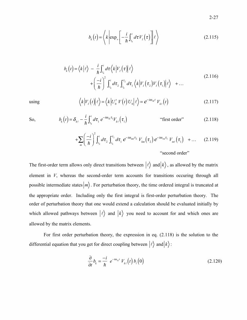
Also note that if the system is initially prepared in a state ! , and a time-dependent

perturbation is turned on and then turned off over the time interval t = !" to+! , then the

complex amplitude in the target state k is just the Fourier transform of V(t) evaluated at the

energy gap !!k

.

bk

t( ) = !i

!d" e

! i#"k"V

k""( )

!$

+$

% (2.123)

If the Fourier transform is defined as

!V !( ) " !F V t( )#$

%& =

1

2'dt V

()

+)

* t( )exp i!t( ) , (2.124)

then P

k!= "V !

k!( )

2

. (2.125)

2-29

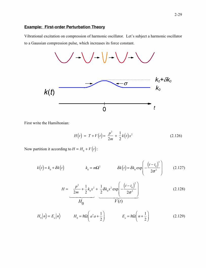
Example: First-order Perturbation Theory

Vibrational excitation on compression of harmonic oscillator. Let’s subject a harmonic oscillator

to a Gaussian compression pulse, which increases its force constant.

First write the Hamiltonian:

H t( ) = T +V t( ) =

p2

2m+

1

2k t( )x2 (2.126)

Now partition it according to H = H

0+V t( ) :

k t( ) = k

0+ !k t( )

k

0= m!

2

!k t( ) = !k0exp "

t " t0( )

2

2# 2

$

%&&

'

())

(2.127)

H =p2

2m+

1

2k

0x2

H0

! "## $##

+1

2!k

0x2 exp "

t " t0( )

2

2# 2

$

%&&

'

())

V (t)! "#### $####

(2.128)

H

0n = E

nn

H0= !! a

†a +

1

2

"#$

%&'

En= !! n +

1

2

"#$

%&'

(2.129)

2-30

If the system is in 0 at

t0= !" , what is the probability of finding it in

n at t = ! ?

For n ! 0 :

bn

t( ) =!i

2!d" V

n0"( )

t0

t

# ei$

n0" (2.130)

Using !

n0= E

n" E

0( ) ! = n# :

bn

t( ) =!i

2!"k

0n x

20 d#

!$

+$

% ein&#

e!# 2

2' 2

(2.131)

So,

bn

t( ) =!i

2!"k

02#$ n x

20 e

!n2$ 2%2 /2 (2.132)

Here we used:

What about the matrix element?

x

2=!

2m!a + a

†( )2

=!

2m!aa + a

†a + aa

†+ a

†a

†( ) (2.133)

First-order perturbation theory won’t allow transitions ton = 1 , only n = 0 andn = 2 .

Generally this wouldn’t be realistic, because you would certainly expect excitation to v=1

would dominate over excitation to v=2. A real system would also be anharmonic, in which case,

the leading term in the expansion of the potential V(x), that is linear in x, would not vanish as it

does for a harmonic oscillator, and this would lead to matrix elements that raise and lower the

excitation by one quantum.

However for the present case,

2 x2

0 = 2!

2m! (2.134)

So,

b2=!i " #k

0$

2m%e!2$ 2%2

(2.135)

2-31

and

P2= b

2

2

=!"k

0

2# 2

2m2$2

e%4# 2$2

= # 2$2!2

"k0

2

k0

2

&

'(

)

*+ e

%4# 2$2

(2.136)

From the exponential argument, significant transfer of amplitude occurs when the compression

pulse is short compared to the vibrational period.

! <<1

" (2.137)

Validity: First order perturbation theory doesn’t allow for bn to change much from its initial

value. For P

2<< 1

! 2"2#2

$k0

2

k0

2

%

&'

(

)* << 1 (2.138)

Generally, the perturbation δk(t) must be small compared to k0, i.e. H

0>> V , but it should also

work well for the impulsive shock limit (σΩ<<1).

2-32

FIRST-ORDER PERTURBATION THEORY

A number of important relationships in quantum mechanics that describe rate processes come

from 1st order perturbation theory. For that, there are a couple of model problems that we want

to work through:

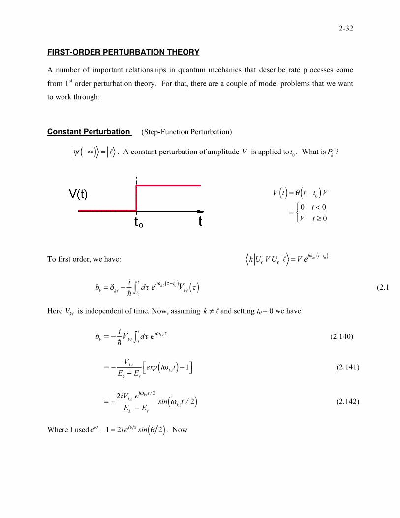
Constant Perturbation (Step-Function Perturbation)

! "#( ) = ! . A constant perturbation of amplitude V is applied to

t0. What is

P

k?

V t( ) = ! t " t0

( )V

=0 t < 0

V t # 0

$%&

To first order, we have:

k U0

†V U

0! =V e

i!k!

t" t0( )

bk= !

k!"

i

"d#

t0

t

$ ei%

k!# "t

0( )V

k!#( ) (2.139)

Here Vk!

is independent of time. Now, assuming k ! ! and setting t0 = 0 we have

bk= !

i

!V

k"d"

0

t

# ei$

k"" (2.140)

= !V

k!

Ek! E

!

exp i"k!

t( ) !1#$

%& (2.141)

= !2iV

k!e

i"k!

t / 2

Ek! E

!

sin "k!

t / 2( ) (2.142)

Where I used e

i!"1= 2i e

i! 2sin ! 2( ) . Now

2-33

Pk= b

k

2

=4 V

k!

2

Ek! E

!

2sin

2 1

2"

k!t (2.143)

Writing this as we did in Lecture 1:

Pk=

V2

!2

sin2!t / !( ) (2.144)

where ! = E

k" E

!( ) 2 . Compare this with the exact result we have for the two-level problem:

Pk=

V2

V2+ !

2sin

2!

2+V

2t / !( ) (2.145)

Clearly the perturbation theory result works for V << Δ.

We can also write the first-order result as

Pk=

V2t

2

!2

sinc2!t / 2!( ) (2.146)

where sinc x( ) = sin x( ) x . Since

limx!0

sinc x( ) = 1,

lim!"0

Pk=V

2t

2!

2 (2.147)

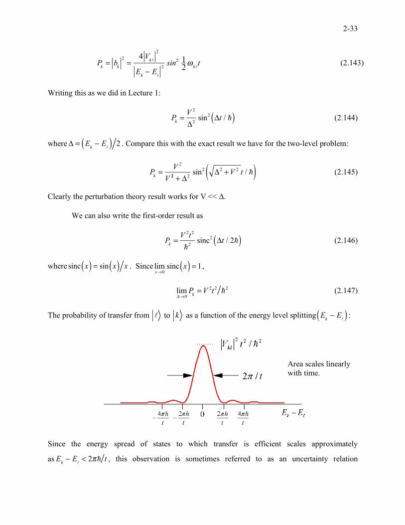
The probability of transfer from ! to

k as a function of the energy level splitting

E

k! E

!( ) :

Since the energy spread of states to which transfer is efficient scales approximately

as E

k! E

!< 2"" t , this observation is sometimes referred to as an uncertainty relation

Area scales linearly with time.

2-34

with !E " !t # 2$! . However, remember that this is really just an observation of the principles

of Fourier transforms, that frequency can only be determined by the length of the time period

over which you observe oscillations. Since time is not an operator, it is not a true uncertainly

relation like !p " !x # 2$! .

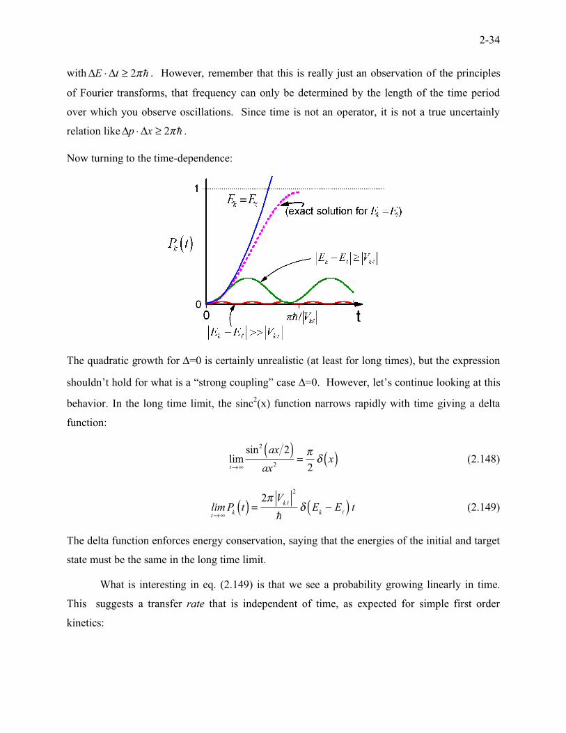
Now turning to the time-dependence:

The quadratic growth for Δ=0 is certainly unrealistic (at least for long times), but the expression

shouldn’t hold for what is a “strong coupling” case Δ=0. However, let’s continue looking at this

behavior. In the long time limit, the sinc2(x) function narrows rapidly with time giving a delta

function:

limt!"

sin2

ax 2( )ax

2=#

2$ x( ) (2.148)

limt!"

Pk

t( ) =2# V

k!

2

"$ E

k% E

!( ) t (2.149)

The delta function enforces energy conservation, saying that the energies of the initial and target

state must be the same in the long time limit.

What is interesting in eq. (2.149) is that we see a probability growing linearly in time.

This suggests a transfer rate that is independent of time, as expected for simple first order

kinetics:

2-35

wk

t( ) =!P

kt( )

!t=

2" Vk!

2

"# E

k$ E

!( ) (2.150)

This is one statement of Fermi’s Golden Rule −the state-to-state form− which describes

relaxation rates from first order perturbation theory. We will show that this rate properly

describes long time exponential relaxation rates that you would expect from the solution

to dP dt = !wP .

2-36

Slowly Applied (Adiabatic) Perturbation

Our perturbation was applied suddenly at t > t0 (step function)

V t( ) = ! t " t

0( )V t( )

This leads to unphysical consequences—you generally can’t turn on a perturbation fast enough

to appear instantaneous. Since first-order P.T. says that the transition amplitude is related to the

Fourier Transform of the perturbation, this leads to additional Fourier components in the spectral

dependence of the perturbation—even for a monochromatic perturbation!

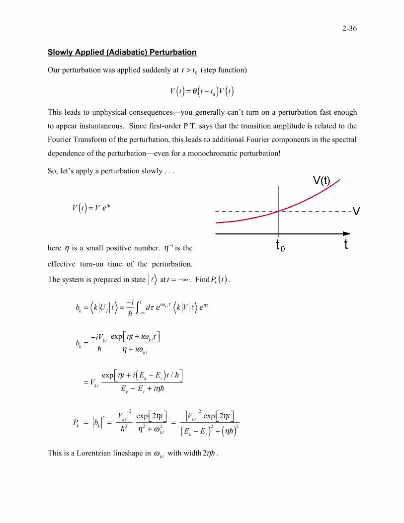
So, let’s apply a perturbation slowly . . .

V t( ) =V e

!t

here η is a small positive number. !"1 is the

effective turn-on time of the perturbation.

The system is prepared in state ! at t = !" . FindP

kt( ) .

bk= k U

I! =

!i

"d" e

i#k!"

!$

t

% k V ! e&"

bk=!iV

k!

"

exp &t + i#k!

t'( )*& + i#

k!

=Vk!

exp &t + i Ek! E

!( )t / "'( )*

Ek! E

!+ i&"

Pk= b

k

2

=V

k!

2

"2

exp 2&t'( )*&2

+#k!

2=

Vk!

2

exp 2&t'( )*

Ek! E

!( )

2

+ &"( )2

This is a Lorentzian lineshape in !

k! with width

2!! .

2-37

Gradually Applied Perturbation Step Response Perturbation

The gradually turned on perturbation has a width dependent on the turn-on rate, and is

independent of time. (The amplitude grows exponentially in time.) Notice, there are no nodes

inPk.

Now, let’s calculate the transition rate:

wkl=!P

k

!t=

Vk!

2

"2

2"e2"t

"2+#

k!

2

Look at the adiabatic limit; !"0 . Setting e2!t

" 1 and using

lim

!" 0

!

!2+#

k!

2= $% #

k!( )

wk!=

2!

"2

Vk!

2

" #k!

( ) =2!

"V

k!

2

" Ek$ E

!( )

We get Fermi’s Golden Rule—independent of how perturbation is introduced!

2-38

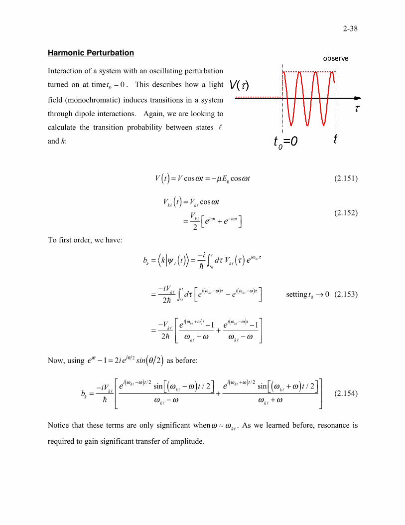
Harmonic Perturbation

Interaction of a system with an oscillating perturbation

turned on at time t0= 0 . This describes how a light

field (monochromatic) induces transitions in a system

through dipole interactions. Again, we are looking to

calculate the transition probability between states !

and k:

V t( ) =V cos!t = "µE

0cos!t (2.151)

Vk!

t( ) =Vk!

cos!t

=V

k!

2e

i! t+ e

" i! t#$

%&

(2.152)

To first order, we have:

bk= k !

It( ) =

"i

!d#

t0

t

$ Vk"

#( ) ei%

k"#

="iV

k"

2!d#

0

t

$ ei %

k"+%( )# " e

i %k""%( )#&

'()

="V

k"

2!

ei %

k"+%( )t "1

%k"+%

+e

i %k""%( )t "1

%k""%

&

'**

(

)++

setting t0! 0 (2.153)

Now, using e

i!"1= 2i e

i! 2sin ! 2( ) as before:

bk=!iV

k!

"

ei "

k!!"( )t / 2

sin "k!!"( )t / 2#

$%&

"k!!"

+e

i "k!+"( )t / 2

sin "k!+"( )t / 2#

$%&

"k!+"

#

$

''

%

&

((

(2.154)

Notice that these terms are only significant when ! "!

k!. As we learned before, resonance is

required to gain significant transfer of amplitude.

2-39

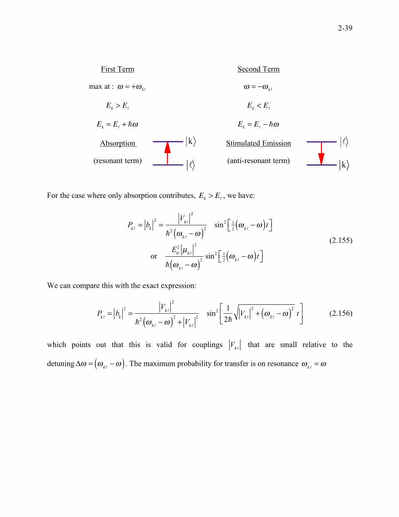
First Term Second Term

max at : ! = +!

k!

! = "!

k!

Ek> E

!

Ek< E

!

Ek= E

!+ "!

Ek= E

!! ""

Absorption Stimulated Emission

(resonant term) (anti-resonant term)

For the case where only absorption contributes, Ek> E

!, we have:

Pk!= b

k

2

=V

k!

2

"2 !

k!"!( )

2sin

2 1

2!

k!"!( )t#

$%&

orE

0

2 µk!

2

" !k!"!( )

2sin

2 1

2!

k!"!( )t#

$%&

(2.155)

We can compare this with the exact expression:

Pk!= b

k

2

=V

k!

2

"2 !

k!"!( )

2

+ Vk!

2sin

21

2"V

k!

2

+ !k!"!( )

2

t#

$%

&

'( (2.156)

which points out that this is valid for couplings V

k! that are small relative to the

detuning !" = "

k!#"( ) . The maximum probability for transfer is on resonance

!

k!=!

2-40

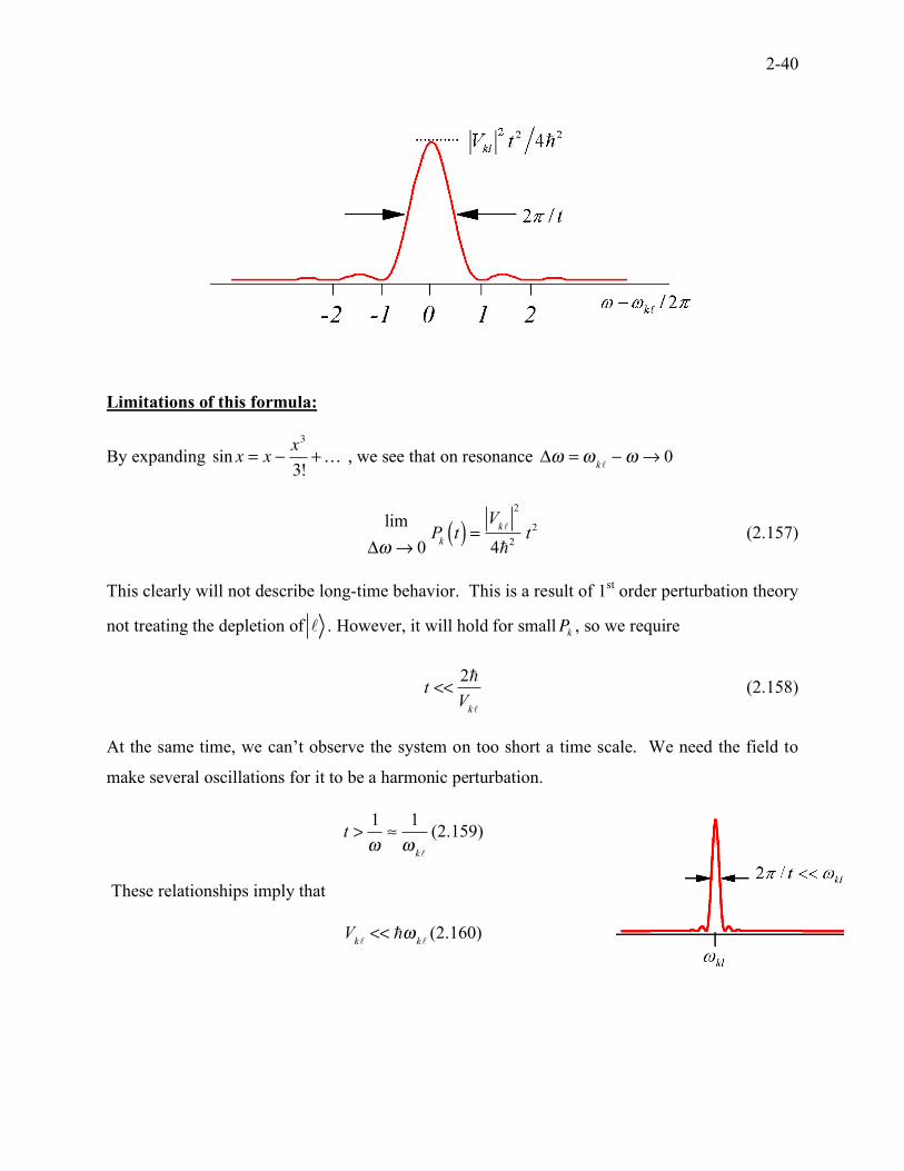
Limitations of this formula:

By expanding

sin x = x !x3

3!+… , we see that on resonance

!" ="

k!# " $ 0

lim

!" # 0P

kt( ) =

Vk!

2

4"2

t2 (2.157)

This clearly will not describe long-time behavior. This is a result of 1st order perturbation theory

not treating the depletion of ! . However, it will hold for smallP

k, so we require

t <<2!

Vk"

(2.158)

At the same time, we can’t observe the system on too short a time scale. We need the field to

make several oscillations for it to be a harmonic perturbation.

t >1

!"

1

!k!

(2.159)

These relationships imply that

V

k!<< "!

k!(2.160)

2-41

Adiabatic Harmonic Perturbation

What happens if we slowly turn on the harmonic interaction?

V t( ) =V e!t

cos"t

bk=#i

!d$

#%

t

& Vk"

ei"

k"$ +!$ e

i"$ + e# i"$

2

'

()

*

+,

=V

k"

2!e!t

ei "

k"+"( )t

# "k"+"( )+ i!

+e

i "k"#"( )t

# "k"#"( ) + i!

'

())

*

+,,

Again, we have a resonant and anti-resonant term, which are now broadened by! . If we only

consider absorption:

Pk= b

k

2

=V

k!

2

4"2

e2!t

1

"k!#"( )

2

+ !2

which is the Lorentzian lineshape centered at !

k!=! with width!" = 2# . Again, we can

calculate the adiabatic limit, setting!" 0 . We will calculate the rate of

transitions !

k!= "P

k/ "t . But let’s restrict ourselves to long enough times that the harmonic

perturbation has cycled a few times (this allows us to neglect cross terms) ! resonances sharpen.

wk!=

!

2"2

Vk!

2

" #k!$#( ) + " #

k!+#( )%

&'(