University of Ljubljanalalg.fri.uni-lj.si/~borut/fct/lib/exe/fetch.php?media=fct-presentation.pdf · Ch 1. Introduction Deﬁnition. (algorithm intuitively) An algorithm for solving

The Foundations of Computability Theory Borut Robič

University of LjubljanaSlovenia, 2015

1

Forward

❖ About Computability Theory

❖ Rules of the game

❖ Exams

2

Contents…

❖ Part I. THE ROOTS OF COMPUTABILITY THEORY❖ Ch 1 Introduction❖ Ch 2 The foundational crisis of mathematics❖ Ch 3 Formalism❖ Ch 4 Hilbert’s attempt at recovery

3

…Contents…

❖ Part II. CLASSICAL COMPUTABILITY THEORY❖ Ch 5 The quest for a formalization❖ Ch 6 The Turing machine❖ Ch 7 The first basic results ❖ Ch 8 Incomputable problems❖ Ch 9 Methods of proving the incomputability

4

…Contents

❖ Part III. RELATIVE COMPUTABILITY

❖ Ch 10 Computation with external help

❖ Ch 11 Degrees of unsolvability

❖ Ch 12 The Turing hierarchy of unsolvability

❖ Ch 13 The class D of degrees of unsolvability

❖ Ch 14 C.E. degrees and the priority method

❖ Ch 15 The arithmetical hierarchy

5

Part I. THE ROOTS OF COMPUTABILITY THEORY

❖ Ch 1 Introduction

❖ Ch 2 The foundational crisis of mathematics

❖ Ch 3 Formalism

❖ Ch 4 Hilbert’s attempt at recovery

6

Ch 1. Introduction❖ Definition. (algorithm intuitively) An algorithm for solving a

problem is a finite set of instructions that lead the processor, in a finite number of steps, from the input data of the problem to the corresponding solution.

Here:❖ algorithm … a finite sequence of instructions

instruction … simple enough, unambiguous, precisely defines the next instruction processor … a device capable of mechanically following, interpreting, and executing instructions while using no self-reflection or external help computation … a sequence of instruction executions (steps)

7

❖ Euclid 325–265 (Eudoxus, 408–355) B.C.E. : Euclid’s algorithm

❖ India 1st–4th century: positional decimal number system

❖ Al-Khwarizmi, 9th century: algorithms for solving equations

❖ Europe 17th century: Schickard, Pascal: the machine for addition/subtraction of natural numbers; Leibniz: the concept of arithmetization (the universal language and computing machine)

❖ Europe 19th century: Babbage’s concept of different programs for different problems (the analytical machine)

Algorithms and Computations Before the 20th Century

❖ The concept of the algorithm remained at the intuitive level. The need for a formal definition arose in the 20th century.

But:

8

Ch 2. The Foundational Crisis of Mathematics

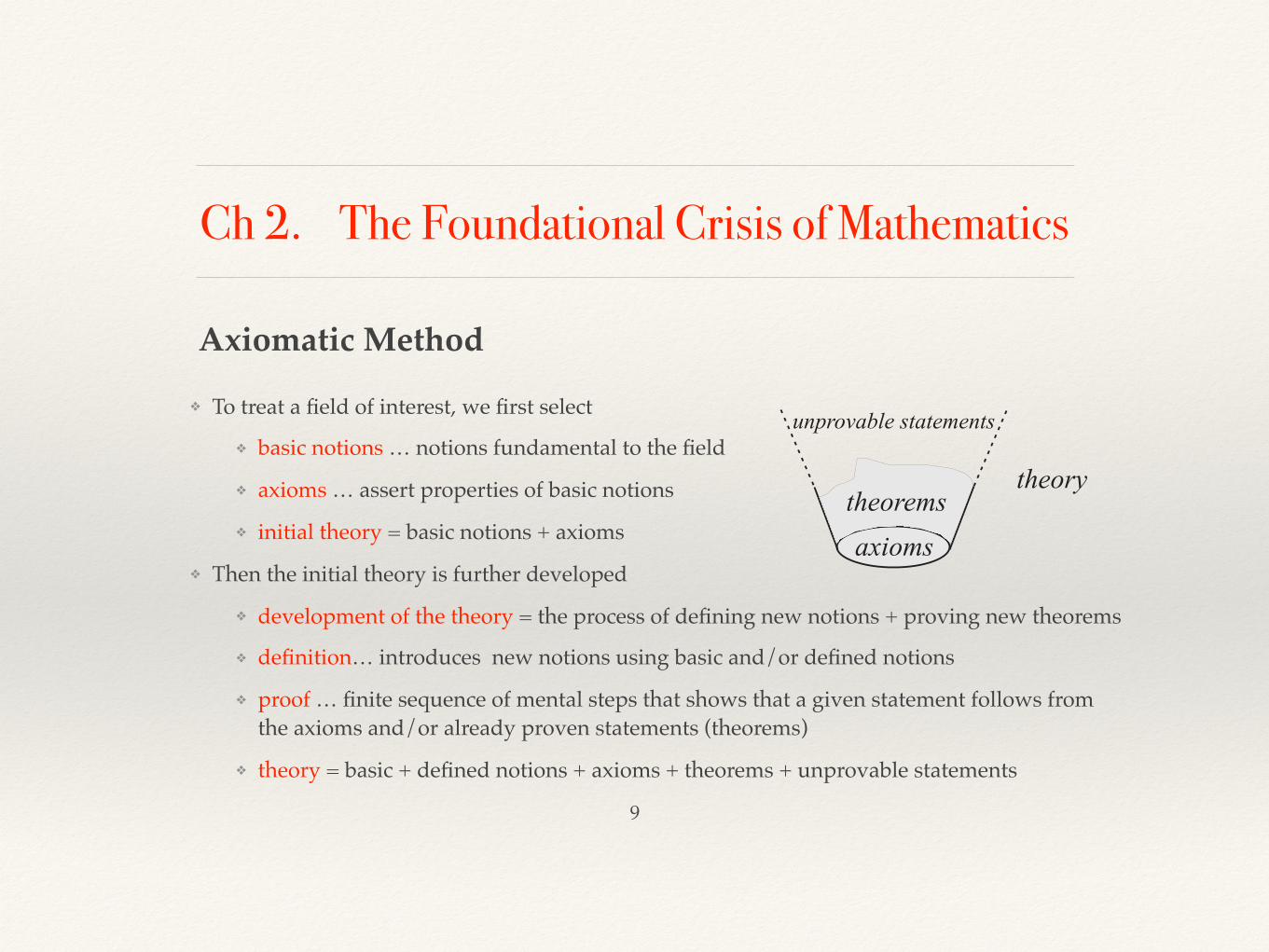
❖ To treat a field of interest, we first select

❖ basic notions … notions fundamental to the field

❖ axioms … assert properties of basic notions

❖ initial theory = basic notions + axioms

❖ Then the initial theory is further developed

❖ development of the theory = the process of defining new notions + proving new theorems

❖ definition… introduces new notions using basic and/or defined notions

❖ proof … finite sequence of mental steps that shows that a given statement follows from the axioms and/or already proven statements (theorems)

❖ theory = basic + defined notions + axioms + theorems + unprovable statements

Axiomatic Method

9

❖ from Euclid to mid-19th century: axioms are evident, i.e., in perfect agreement with human experience in the field of interest

❖ but, in the 19th century: experience and intuition can be misleading

❖ e.g., Euclid’s fifth axiom (Parallel Postulate), although self-evident, has alternatives; these give rise to non-Euclidean geometries, parts of reality!

Evident Axiomatic Systems

Hypothetical Axiomatic Systems

❖ basic notions … their real nature is no longer important❖ axioms = hypotheses; needn’t be self-evident/in agreement with reality ❖ there is no obvious link between the theory and reality❖ the reasonableness and usefulness of the theory depends on the

successful interpretations (applications of theory on parts of reality)

10

❖ Basic notions

❖ (Cantor’s set) A set is any collection of definite, distinguishable objects of our intuition or of our intellect to be conceived as a whole.

❖ (Membership relation ∈) A member of a set is any object that is in the set. An object either is or it is not a member of the set. (Law of Excluded Middle)

❖ Axioms

❖ (Extensionality) A set is completely determined by its members.

❖ e.g., S = {a, b, c} or S = {x|x has property P} = {x|P(x)}

❖ (Abstraction) Every property determines a set.

❖ (Choice) Given any set F of nonempty pairwise disjoint sets, there is a set that contains exactly one member of each set in F.

Cantor’s Naive Set Theory

11

❖ New, defined notions

❖ relations between sets: = (equality of sets), ⊆ (subset of a set)

❖ operations on sets: complement, ∪ (union), ∩ (intersection), - (difference), and 2* (power set of a set)

❖ and using the above:

• ordered pair, Cartesian product, function (injective, surjective, bijective)

• natural number

• cardinal number (describing the size of a set)

• ordinal number (describing the order in a set)

❖ … but also surprising theorems

❖ e.g., There are larger and larger infinite sets whose sizes are larger and larger infinite cardinal numbers—and this never ends!

❖ Cantor’s set theory was useful but curious, wild world of infinities!12

… cont’d (Cantor’s Naive Set Theory)

Paradoxes in Cantor’s Set Theory

❖ Logical paradoxes

❖ In Cantor’s set theory, paradoxical statements were proved, e.g.,

• there is an ordered set Ω whose ordinal number is larger than itself ! (Burali-Forti)

• there is a set U whose cardinal number is larger than itself ! (Cantor himself)

• there is a set R that both is and is not a member of itself! (Russell)

❖ Why do we fear paradoxes?

❖ If, in a theory, a statement and its negation can be proved, then any statement of the theory can be proved. Such a theory has no cognitive value!

13

❖ Intuitionism

❖ Brouwer, Heyting, …

❖ Demanded for mathematical rigour, e.g.,

• infinite sets are potentialities, not actualities

• to exist is the same as to be constructed

• the Law of Excluded Middle is not fully accepted

• Logicism

❖ Boole, Frege, Peano, Peirce, Russell, Whitehead

❖ Developed symbolic language for concise/precise mathematical expression, e.g.,

• algebraic logic, Propositional Calculus P

• rules of construction, quantified variables, First-order Logic L

• Principia Mathematica, a theory containing fundamental theorems of mathematics in symbolic language

Schools of Recovery

14

❖ Formalism

❖ Hilbert, Ackermann, Bernays, …

❖ Focussed on the syntax of math. expressions instead of their semantics

• defined rules to build well-formed objects from symbols

• invented formal axiomatic systems to implement these ideas

❖ A formal axiomatic system consists of

• a symbolic language

• + rules of construction (to build formulas, well-formed expressions)

• + rules of inference (to build formal proofs, w.f. sequences of formulas)

• Some formulas are axioms. A formal proof is a finite sequence of formulas each of which is inferred from axioms and/or previous formulas only. A theorem is a formula that can be formally proved.

❖ A (formal) theory = axioms + theorems + other formulas15

… cont’d (Schools of Recovery)

❖ Interpretation

• a theory must be given some meaning (interpreted in a field of interest)

• this tells us whether the theory is applicable

❖ Metatheory

• answers the questions about the formal theory

• e.g., Is the formal theory consistent? Is it complete? Is it decidable?

❖ Goals of formalism

• short term:

- Is Principia Mathematica a consistent theory? Is it complete?

• long term:

- develop all mathematics in one formal axiomatic system and prove that such mathematics is free of all (un)known paradoxes

16

… cont’d (Formalism)

… cont’d (Schools of Recovery)

Ch 3. Formalism

17

❖ = symbolic language + axioms + rules of inference

❖ Symbolic language

❖ = alphabet + rules of construction

❖ alphabet = individual-constant symbols a,b,c,… + individual-variable symbols x,y,x,… + function symbols f,g,h,… + predicate symbols P,Q,R,… + logical connectives ⋀,⋁,⇒,⇔,¬ + quantification symbols ∀,∃ + punctuation marks (+ function-variable symbols + predicate-variable symbols)

❖ rules of construction: define terms and formulas, i.e., well-formed sequences of symbols

Formal Axiomatic System

17

❖ Axioms

❖ = selected formulas = logical axioms + proper axioms❖ logical axioms: epitomize the principles of pure logic reflection❖ proper axioms: condense other special basic notions and facts

❖ Rules of inference

❖ specify conditions in which, given a set of premises, one may derive a conclusion❖ e.g., Modus Ponens: G, G⇒F ⊢ F and Generalization: F(x) ⊢ ∀F(x)

❖ Development of the theory

❖ starts when the symbolic language, axioms, and rules of inference are fixed ❖ each new notion must be defined by the basic and/or already defined notions

❖ each new proposition must be derived (formally proved) to become a theorem❖ ⊢

F F … denotes that F is derivable (formally provable) in the theory (f.a.s) F

❖ Benefits ❖ it is in principle easier to maintain and check the validity of formal proofs

18

… cont’d (Formal Axiomatic System)

❖ Interpretation of a Theory

❖ assigns a particular meaning to a (formal) theory in a particular domain, i.e., describes, for every closed formula of the theory, how the formula is to be understood as a statement about members, functions, and relations of the domain

❖ an open formula (one with free individual-varible symbols) is

• satisfiable if these symbols can be assigned values so that the resulting statement is true

• valid under the (current) interpretation if any assignment of values to these symbols results in a true statement

❖ a theory may have several interpretations

❖ a formula is logically valid if it is valid under every interpretation

• logical axioms are logically valid; what about proper axioms?

Interpretations and Models

19

❖ Model of a Theory

❖ a model of a theory = an interpretation of the theory under which also all proper axioms are valid (hence, all axioms are valid)

❖ intuitively: a model of the theory is a field of our interest that the theory sensibly formalizes

❖ a theory may have several models

❖ a formula is valid in the theory if it is valid in every model of the theory

• intuitively: such a formula represents a (mathematical) Truth expressible in the formal axiomatic system (theory)

• ⊨F F … denotes that F is valid in the theory (f.a.s.) F

20

… cont’d (Interpretations and Models)

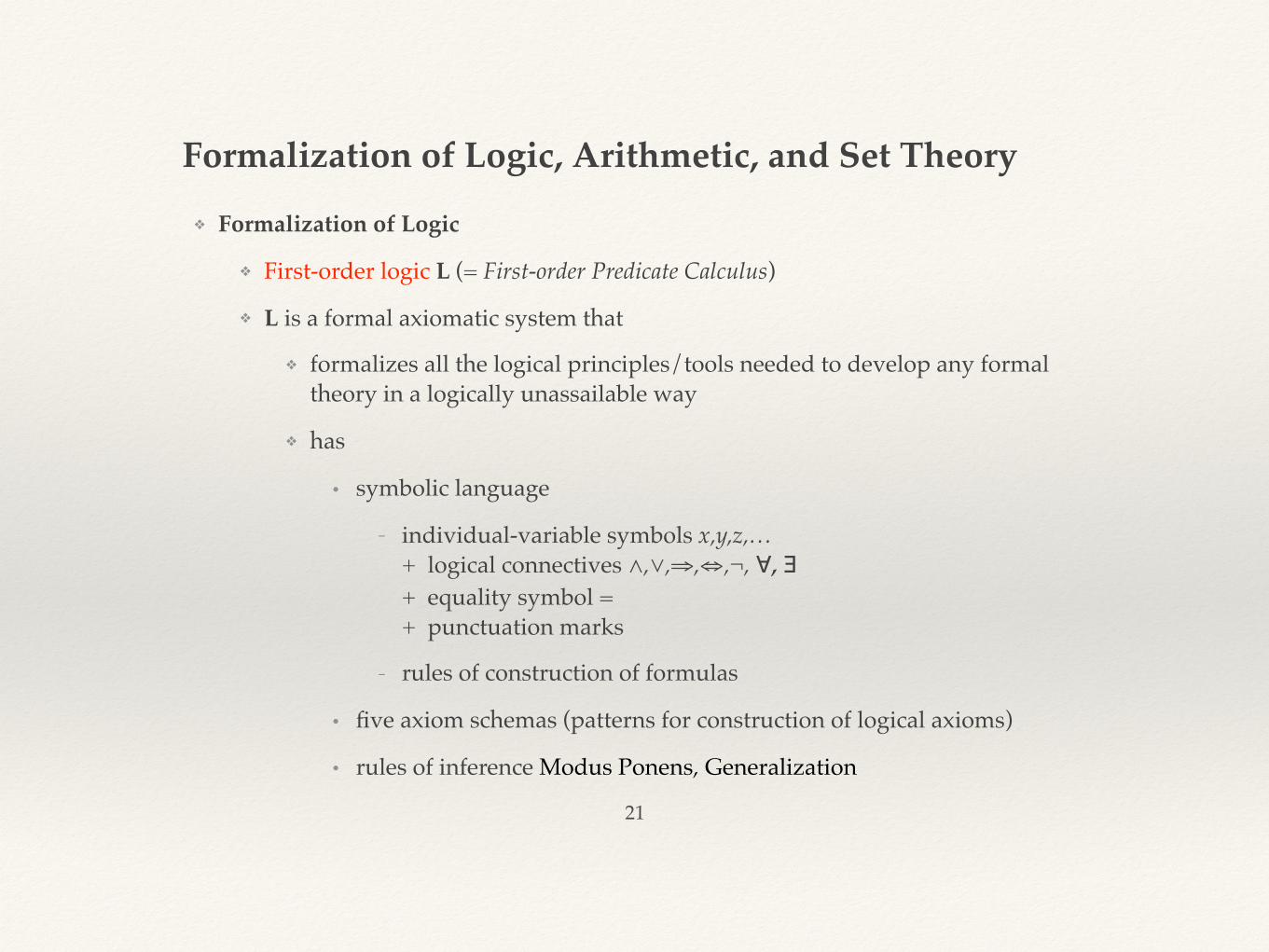
❖ Formalization of Logic

❖ First-order logic L (= First-order Predicate Calculus)

❖ L is a formal axiomatic system that

❖ formalizes all the logical principles/tools needed to develop any formal theory in a logically unassailable way

❖ has

• symbolic language

- individual-variable symbols x,y,z,… + logical connectives ⋀,⋁,⇒,⇔,¬, ∀, ∃ + equality symbol = + punctuation marks

- rules of construction of formulas

• five axiom schemas (patterns for construction of logical axioms)

• rules of inference Modus Ponens, Generalization

Formalization of Logic, Arithmetic, and Set Theory

21

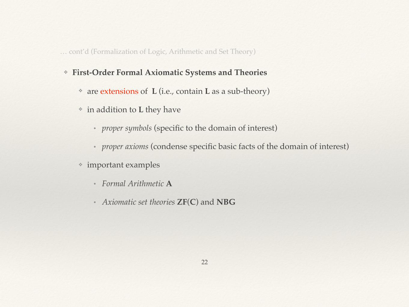
❖ First-Order Formal Axiomatic Systems and Theories

❖ are extensions of L (i.e., contain L as a sub-theory)

❖ in addition to L they have

• proper symbols (specific to the domain of interest)

• proper axioms (condense specific basic facts of the domain of interest)

❖ important examples

• Formal Arithmetic A

• Axiomatic set theories ZF(C) and NBG

22

… cont’d (Formalization of Logic, Arithmetic and Set Theory)

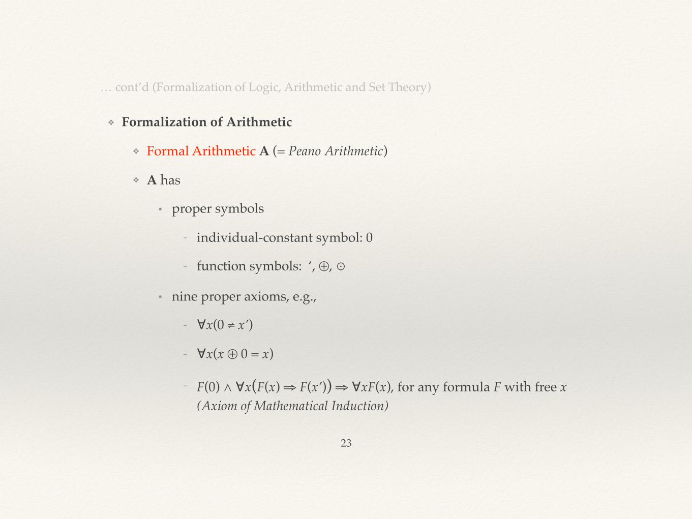
❖ Formalization of Arithmetic

❖ Formal Arithmetic A (= Peano Arithmetic)

❖ A has

• proper symbols

- individual-constant symbol: 0

- function symbols: ‘, ⊕, ⊙

• nine proper axioms, e.g.,

- ∀x(0 ≠ x’)

- ∀x(x ⊕ 0 = x)

- F(0) ⋀ ∀x(F(x) ⇒ F(x’)) ⇒ ∀xF(x), for any formula F with free x (Axiom of Mathematical Induction)

23


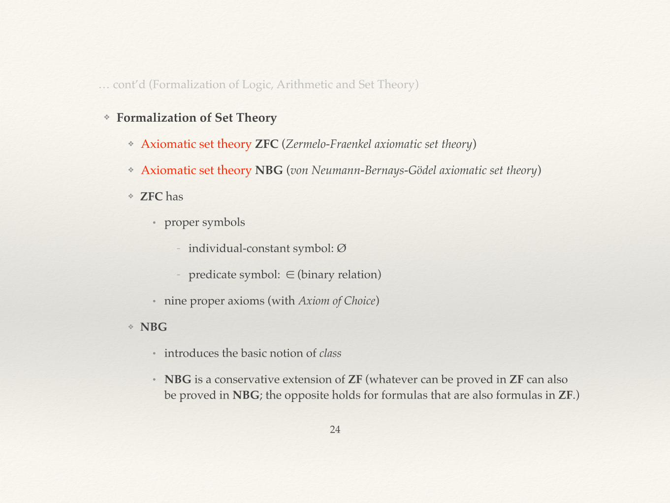
❖ Formalization of Set Theory

❖ Axiomatic set theory ZFC (Zermelo-Fraenkel axiomatic set theory)

❖ Axiomatic set theory NBG (von Neumann-Bernays-Gödel axiomatic set theory)

❖ ZFC has

• proper symbols

- individual-constant symbol: Ø

- predicate symbol: ∈ (binary relation)

• nine proper axioms (with Axiom of Choice)

❖ NBG

• introduces the basic notion of class

• NBG is a conservative extension of ZF (whatever can be proved in ZF can also be proved in NBG; the opposite holds for formulas that are also formulas in ZF.)

24


Ch 4. Hilbert’s Attempt at Recovery

25

❖ = a promising formalistic attempt to recover mathematics❖ David Hilbert

❖ Main ideas

❖ use formal axiomatic systems to put mathematics on a sound footing

❖ to achieve that

❖ define certain fundamental problems about f.a.s. and their theories❖ construct a f.a.s. M that will formalize all mathematics

❖ solve (positively) the fundamental problems for the case of M

25

Hilbert’s Program

25

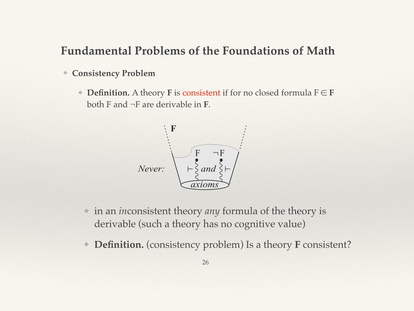
❖ Consistency Problem

❖ Definition. A theory F is consistent if for no closed formula F ∈ F both F and ¬F are derivable in F.

Fundamental Problems of the Foundations of Math

26

❖ in an inconsistent theory any formula of the theory is derivable (such a theory has no cognitive value)

❖ Definition. (consistency problem) Is a theory F consistent?

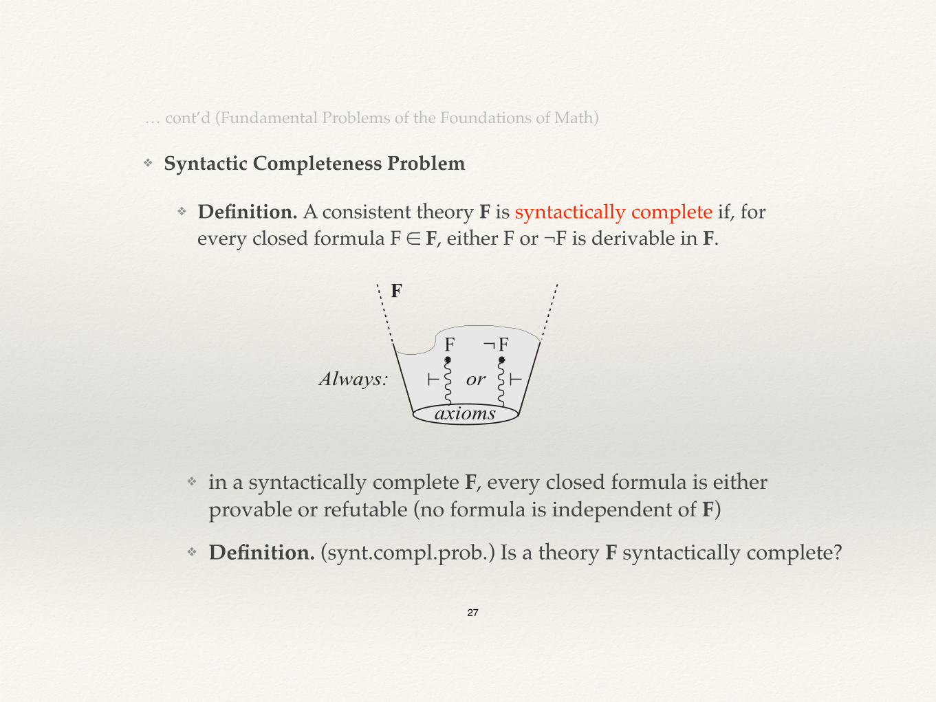
❖ Syntactic Completeness Problem

❖ Definition. A consistent theory F is syntactically complete if, for every closed formula F ∈ F, either F or ¬F is derivable in F.

… cont’d (Fundamental Problems of the Foundations of Math)

❖ in a syntactically complete F, every closed formula is either provable or refutable (no formula is independent of F)

❖ Definition. (synt.compl.prob.) Is a theory F syntactically complete?

27

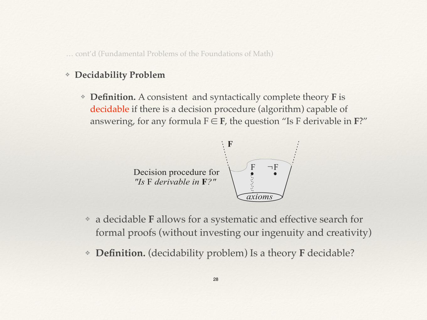
❖ Decidability Problem

❖ Definition. A consistent and syntactically complete theory F is decidable if there is a decision procedure (algorithm) capable of answering, for any formula F ∈ F, the question “Is F derivable in F?”


❖ a decidable F allows for a systematic and effective search for formal proofs (without investing our ingenuity and creativity)

❖ Definition. (decidability problem) Is a theory F decidable?

28

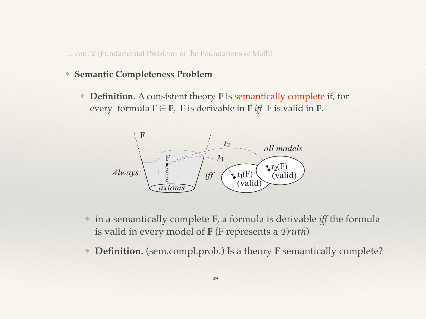
❖ Semantic Completeness Problem

❖ Definition. A consistent theory F is semantically complete if, for every formula F ∈ F, F is derivable in F iff F is valid in F.


❖ in a semantically complete F, a formula is derivable iff the formula is valid in every model of F (F represents a Truth)

❖ Definition. (sem.compl.prob.) Is a theory F semantically complete?

29

❖ Program

❖ A. Find a f.a.s. M capable of deriving all theorems of mathematics.

❖ B. Prove that the theory M is semantically complete.

❖ C. Prove that the theory M is consistent.

❖ D. Construct an algorithm that is a decision procedure for the theory M.

Hilbert’s Program

30

❖ Having attained A,B,C,D, every mathematical statement would be mechanically verifiable. Why? Let be given an arbitrary mathematical statement. Then:

❖ 1. write the statement as a formula F ∈ M ❖ 2. since M is semantically complete (B.), F is valid in M iff F is derivable in M❖ 3. since M is consistent (C.), F and ¬F are not both derivable❖ 4. apply the decision procedure (D.) to decide which of F and ¬F is derivable❖ Conclusion: if F is derivable, the statement is a Truth in math; otherwise, it is not❖ Note. Hilbert expected that M would be syntactically complete!

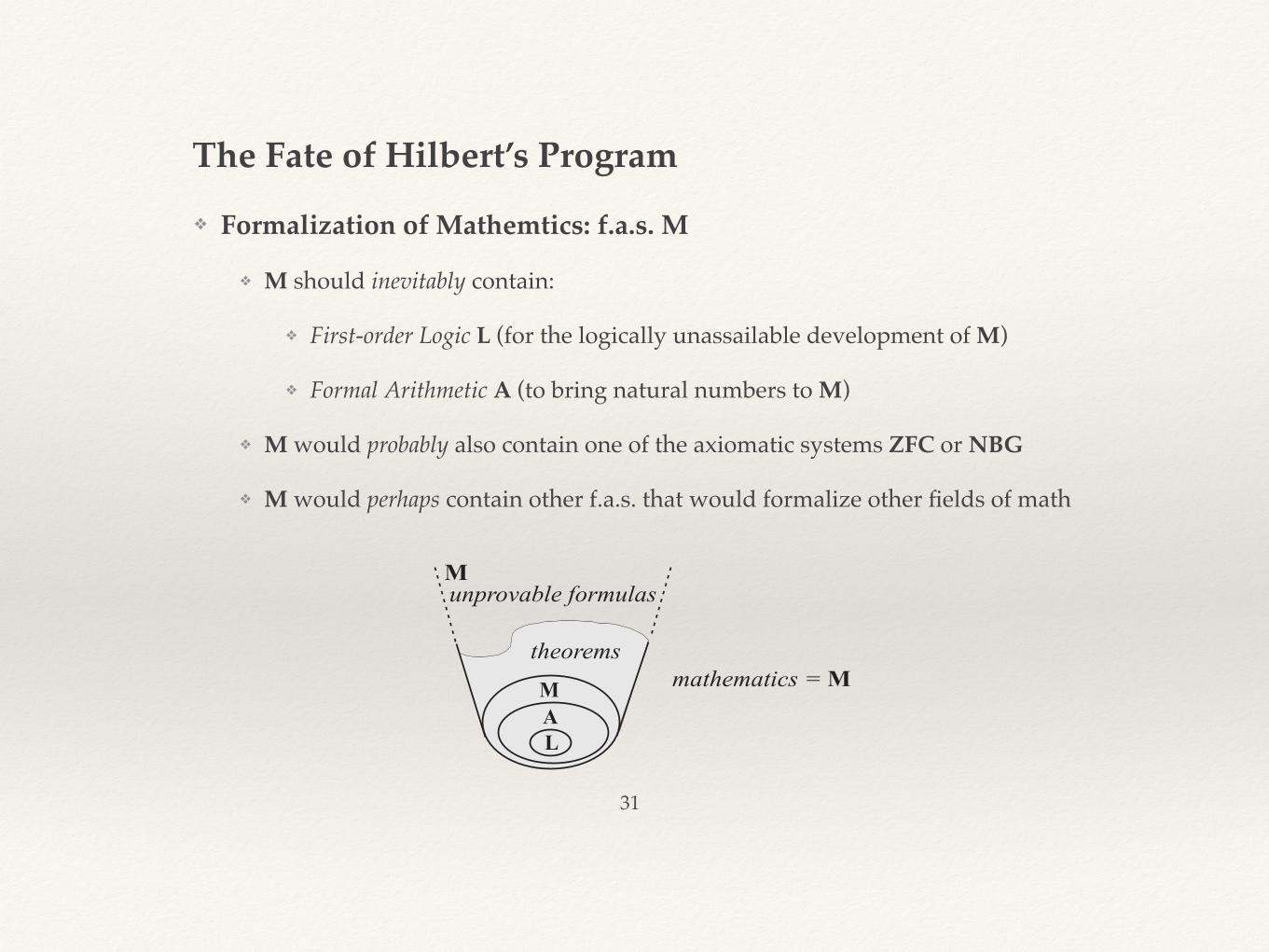
❖ Formalization of Mathemtics: f.a.s. M

❖ M should inevitably contain:

❖ First-order Logic L (for the logically unassailable development of M)

❖ Formal Arithmetic A (to bring natural numbers to M)

❖ M would probably also contain one of the axiomatic systems ZFC or NBG

❖ M would perhaps contain other f.a.s. that would formalize other fields of math

The Fate of Hilbert’s Program

31

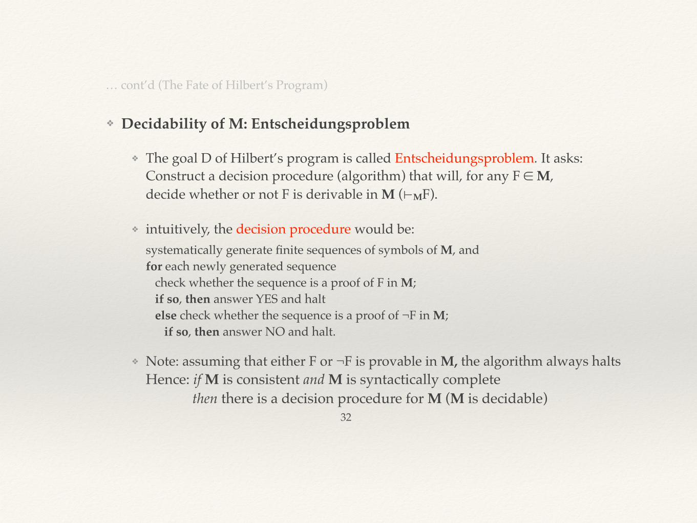
❖ Decidability of M: Entscheidungsproblem

❖ The goal D of Hilbert’s program is called Entscheidungsproblem. It asks: Construct a decision procedure (algorithm) that will, for any F ∈ M, decide whether or not F is derivable in M (⊢MF).

❖ intuitively, the decision procedure would be:

… cont’d (The Fate of Hilbert’s Program)

32

systematically generate finite sequences of symbols of M, andfor each newly generated sequence check whether the sequence is a proof of F in M; if so, then answer YES and halt else check whether the sequence is a proof of ¬F in M; if so, then answer NO and halt.

❖ Note: assuming that either F or ¬F is provable in M, the algorithm always haltsHence: if M is consistent and M is syntactically complete then there is a decision procedure for M (M is decidable)

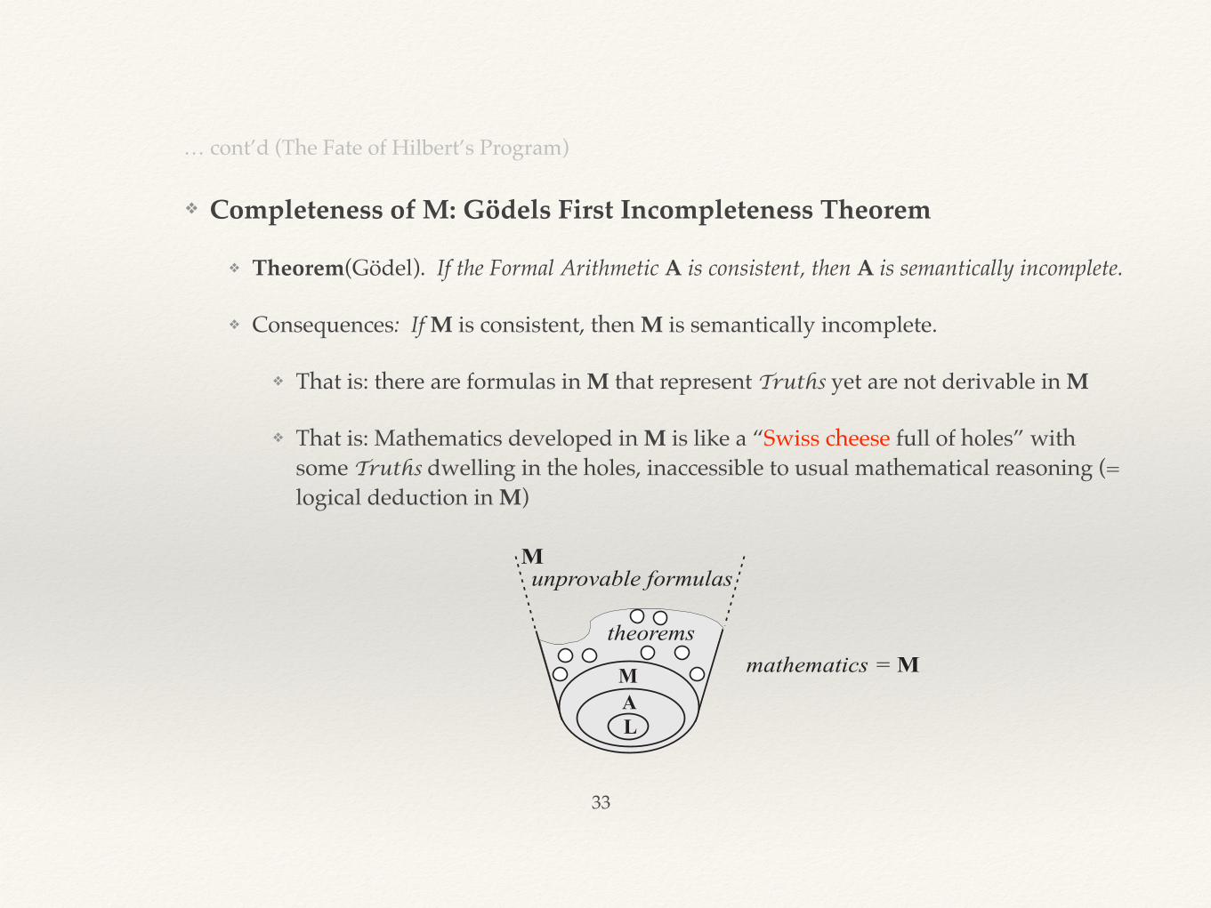
❖ Completeness of M: Gödels First Incompleteness Theorem

❖ Theorem(Gödel). If the Formal Arithmetic A is consistent, then A is semantically incomplete.

❖ Consequences: If M is consistent, then M is semantically incomplete.

❖ That is: there are formulas in M that represent Truths yet are not derivable in M

❖ That is: Mathematics developed in M is like a “Swiss cheese full of holes” with some Truths dwelling in the holes, inaccessible to usual mathematical reasoning (= logical deduction in M)


33

❖ Consistency of M: Gödels Second Incompleteness Theorem

❖ Theorem(Gödel). If the Formal Arithmetic A is consistent, then this cannot be proved in A.

❖ Consequences: Proving the consistency of A would require means that are more complex (and less transparent) than those available in A.

❖ E.g., Gentzen (1936) proved that A is consistent by using transfinite induction

❖ So, we believe that A is consistent.

❖ But this does not imply that M would be consistent!

❖ Why? There is a generalization of Gödel’s theorem: If a consistent theory F contains A, then the consistency of F cannot be proved within F. (Take F := M.)


34

❖ Legacy of Hilbert’s Program

❖ The mechanical, syntax-directed development of mathematics within the framework of formal axiomatic systems may be safe from paradoxes, but such mathematics suffers from semantic incompleteness and the lack of a possibility of proving its consistency.

❖ Thus, Hilbert’s program failed.


35

❖ The problem of finding an algorithm that is a decision procedure for a given theory remained topical.

❖ Since there was a possibility of non-existence of such an algorithm, a formalization of the concept of the algorithm became necessary.

However:

Part II. CLASSICAL COMPUTABILITY THEORY

❖ Ch 5 The quest for a formalization

❖ Ch 6 The Turing machine

❖ Ch 7 The first basic results

❖ Ch 8 Incomputable problems

❖ Ch 9 Methods of proving the in computability

36

Ch 5. The Quest for a Formalization

37

❖ Is there some other algorithmic way of recognizing every mathematical Truth?❖ But, what is algorithm, anyway?

❖ Definition. An algorithm (intuitively) for solving a problem is a finite set of instructions that lead the processor, in a finite number of steps, from the input data of the problem to the corresponding solution.

❖ Questions. What instructions should be basic (i.e., allowed)? Would they suffice to compose any algorithm? Would they execute in a discrete or continuous way? Would their results be predictable (deterministic) or not? Could the processor execute any basic instruction? Where would be kept the algorithm, input data, intermediate and final results? …

3737

What is an Algorithm? What Do We Mean by Computation?

37

❖ Definition. A definition that formally describes and characterises the basic notions of algorithmic computation (i.e., the algorithm and its environment) is called the model of computation.

❖ What could a model of computation take as an example?

❖ Modelling after functions

• Recursive functions

• General recursive functions

• Lambda-calculus

❖ Modelling after humans

• Turing machine

❖ Modelling after languages

• Post machine

• Markov algorithms

Models of Computation

38

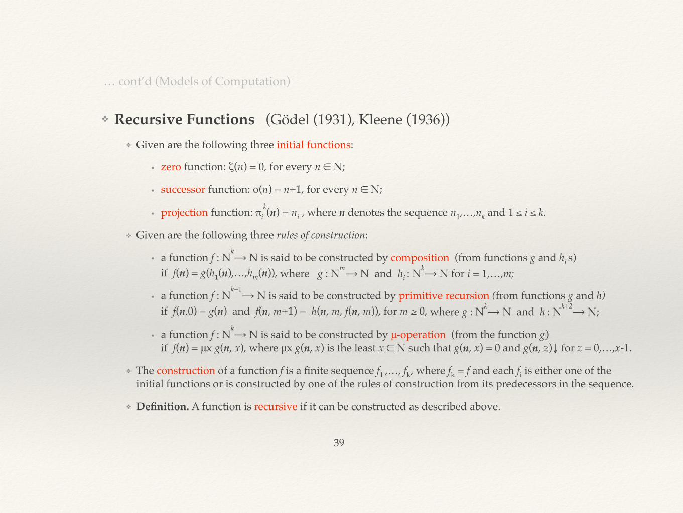
❖ Recursive Functions (Gödel (1931), Kleene (1936))❖ Given are the following three initial functions:

• zero function: ζ(n) = 0, for every n ∈ N;

• successor function: σ(n) = n+1, for every n ∈ N;

• projection function: πik(n) = ni , where n denotes the sequence n1,…,nk and 1 ≤ i ≤ k.

❖ Given are the following three rules of construction:

• a function f : Nk⟶ N is said to be constructed by composition (from functions g and hi s)

if f(n) = g(h1(n),…,hm(n)), where g : Nm⟶ N and hi : Nk⟶ N for i = 1,…,m;

• a function f : Nk+1⟶ N is said to be constructed by primitive recursion (from functions g and h)

if f(n,0) = g(n) and f(n, m+1) = h(n, m, f(n, m)), for m ≥ 0, where g : Nk⟶ N and h : Nk+2⟶ N;

• a function f : Nk⟶ N is said to be constructed by μ-operation (from the function g)

if f(n) = μx g(n, x), where μx g(n, x) is the least x ∈ N such that g(n, x) = 0 and g(n, z)↓ for z = 0,…,x-1.

❖ The construction of a function f is a finite sequence f1 ,…, fk, where fk = f and each fi is either one of the initial functions or is constructed by one of the rules of construction from its predecessors in the sequence.

❖ Definition. A function is recursive if it can be constructed as described above.

… cont’d (Models of Computation)

39

❖ Model of computation (Gödel-Kleene)

❖ an “algorithm” is a construction of a recursive function

❖ a “computation” is a calculation of a value of a recursive function that proceeds according to the construction of the function

❖ a “computable” function is a recursive function


40

❖ General Recursive Functions (Herbrand(1931), Gödel (1934))

❖ Let f denote an unknown function and let g1 ,…, gk be known numerical functions.

❖ Let E(f) denote a system of equations (with f and gs) which

• is in standard form, i.e.,

- f is only allowed on the left-hand side of the equations, and

- f must appear as f(gi(…), …, gj(…)) = …

• guarantees that f is a well-defined function.

❖ There are two rules for manipulating E(f) to calculate the value of f :

• in an equation, all occurrences of a variable can be substituted by the same number

• in an equation, an occurrence of a function can be replaced by its value

❖ The system E(f) defines the function f.

❖ Definition. A function is general recursive if there is a system that defines it.


41

❖ Model of computation (Herbrand-Gödel-Kleene)

❖ an “algorithm” is a system of equations E(f) for some f

❖ a “computation” is a calculation of a value of a general recursive function f that proceeds according to E(f) and the two rules

❖ a “computable” function is a general recursive function


42

❖ Lambda-Calculus (Church (1931-34))

❖ Let f, g, x, y, z, … denote variables.

❖ A λ-term is a well-formed expression defined inductively as follows:

• a variable is a λ-term (called atom)

• if M is a λ-term and x a variable, then (λx.M) is a λ-term (built from M by abstraction)

• if M and N are λ-terms, then (MN) is a λ-term (called the application of M on N)

❖ λ-terms can be transformed into other λ-terms. A transformation is a series of one-step transformations called β-reductions. There are two rules to do a β-reduction:

• α-conversion renames a bound variable in a λ-term i

• β-contraction transforms a λ-term (λx.M)N —called β-redex— into a λ-term obtained from M by substituting N for every bound occurrence of x in M. (We say that M is applied on N.)

❖ When a λ-term contains no β-redexes, it cannot further be β-reduced; such a λ-term is said to be in β-normal form. (Intuitively, a λ-term is in β-normal form if it contains no functions to apply.)

❖ Definition. A function is λ-definable if it can be represented by a λ-term.


43

❖ Model of computation (Church)

❖ an “algorithm” is a λ-term

❖ a “computation” is a transformation of an initial λ-term into the final one

❖ a “computable” function is a λ-definable function


44

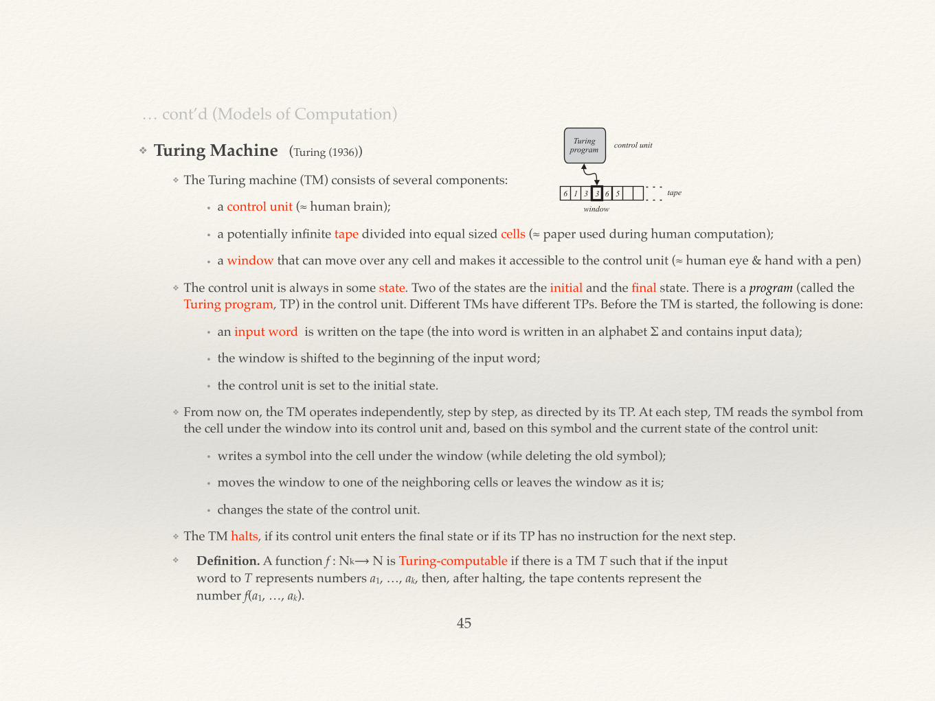
❖ Turing Machine (Turing (1936))

❖ The Turing machine (TM) consists of several components:

• a control unit (≈ human brain);

• a potentially infinite tape divided into equal sized cells (≈ paper used during human computation);

• a window that can move over any cell and makes it accessible to the control unit (≈ human eye & hand with a pen)

❖ The control unit is always in some state. Two of the states are the initial and the final state. There is a program (called the Turing program, TP) in the control unit. Different TMs have different TPs. Before the TM is started, the following is done:

• an input word is written on the tape (the into word is written in an alphabet Σ and contains input data);

• the window is shifted to the beginning of the input word;

• the control unit is set to the initial state.

❖ From now on, the TM operates independently, step by step, as directed by its TP. At each step, TM reads the symbol from the cell under the window into its control unit and, based on this symbol and the current state of the control unit:

• writes a symbol into the cell under the window (while deleting the old symbol);

• moves the window to one of the neighboring cells or leaves the window as it is;

• changes the state of the control unit.

❖ The TM halts, if its control unit enters the final state or if its TP has no instruction for the next step.


45

❖ Definition. A function f : Nk⟶ N is Turing-computable if there is a TM T such that if the input word to T represents numbers a1, …, ak, then, after halting, the tape contents represent the number f(a1, …, ak).

❖ Model of computation (Turing)

❖ an “algorithm” is a Turing program

❖ a “computation” is an execution of a Turing program on a Turing machine

❖ a “computable” function is a Turing-computable function


46

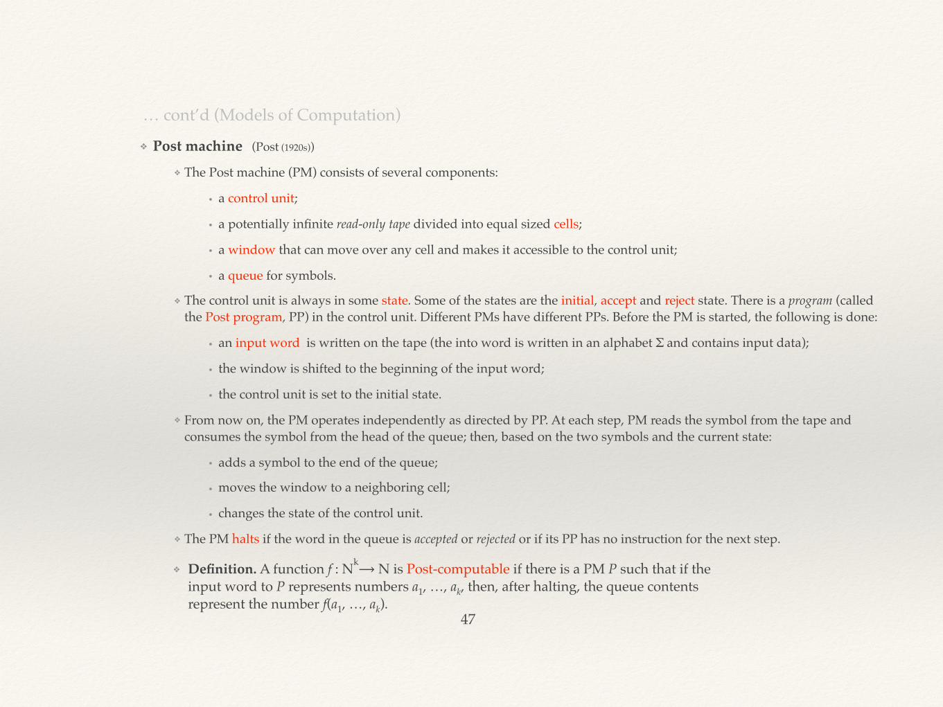
❖ Post machine (Post (1920s))

❖ The Post machine (PM) consists of several components:

• a control unit;

• a potentially infinite read-only tape divided into equal sized cells;

• a window that can move over any cell and makes it accessible to the control unit;

• a queue for symbols.

❖ The control unit is always in some state. Some of the states are the initial, accept and reject state. There is a program (called the Post program, PP) in the control unit. Different PMs have different PPs. Before the PM is started, the following is done:

• an input word is written on the tape (the into word is written in an alphabet Σ and contains input data);

• the window is shifted to the beginning of the input word;


❖ From now on, the PM operates independently as directed by PP. At each step, PM reads the symbol from the tape and consumes the symbol from the head of the queue; then, based on the two symbols and the current state:

• adds a symbol to the end of the queue;

• moves the window to a neighboring cell;

• changes the state of the control unit.

❖ The PM halts if the word in the queue is accepted or rejected or if its PP has no instruction for the next step.


47

❖ Definition. A function f : Nk⟶ N is Post-computable if there is a PM P such that if the input word to P represents numbers a1, …, ak, then, after halting, the queue contents represent the number f(a1, …, ak).

❖ Model of computation (Post)

❖ an “algorithm” is a Post program

❖ a “computation” is an execution of a Post program on a Post machine

❖ a “computable” function is a Post-computable function


48

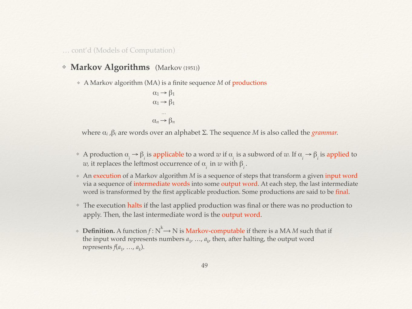
❖ Markov Algorithms (Markov (1951))

❖ A Markov algorithm (MA) is a finite sequence M of productions


49

❖ Definition. A function f : Nk⟶ N is Markov-computable if there is a MA M such that if the input word represents numbers a1, …, ak, then, after halting, the output word represents f(a1, …, ak).

α1 → β1

α1 → β1

…

αn → βn

where αi ,βi are words over an alphabet Σ. The sequence M is also called the grammar.

❖ A production αi → β

i is applicable to a word w if α

i is a subword of w. If α

i → β

i is applied to

w, it replaces the leftmost occurrence of αi in w with β

i .

❖ An execution of a Markov algorithm M is a sequence of steps that transform a given input word via a sequence of intermediate words into some output word. At each step, the last intermediate word is transformed by the first applicable production. Some productions are said to be final.

❖ The execution halts if the last applied production was final or there was no production to apply. Then, the last intermediate word is the output word.

❖ Model of computation (Markov)

❖ an “algorithm” is a Markov algorithm (grammar)

❖ a “computation” is an execution of a Markov algorithm

❖ a “computable” function is a Markov-computable function


50

❖ Which model (if any) is the right one, i.e., which appropriately formalises (⟷) the intuitive concepts of the “algorithm,” “computation,” and “computable” function?

❖ Speculations:

• Church thesis (1936): λ-calculus is the right one.

• Turing thesis (1936) : Turing machine is the right one

❖ But we cannot prove that (a vague concept A) ⟷ (a rigorous concept B) !!

❖ Luckily, the (rigorously defined) models of computation were proved to be equivalent in the sense that what can be computed by one of them can also be computed by any other.

❖ This strengthened the belief in the following Computability Thesis:

Computability (Church-Turing) Thesis

51

Basic intuitive concepts of computing are appropriately formalised as follows: “algorithm” ⟷ Turing program “computation” ⟷ execution of a Turing program on a Turing machine “computable” function ⟷ Turing-computable function Instead of the TM we can use any other equivalent model.

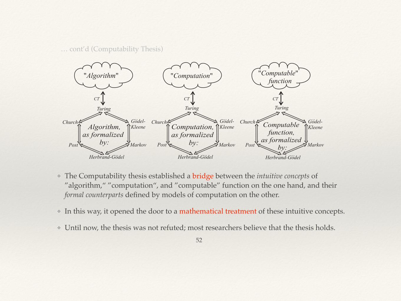
❖ The Computability thesis established a bridge between the intuitive concepts of ”algorithm,“ ”computation“, and ”computable” function on the one hand, and their formal counterparts defined by models of computation on the other.

❖ In this way, it opened the door to a mathematical treatment of these intuitive concepts.

❖ Until now, the thesis was not refuted; most researchers believe that the thesis holds.

… cont’d (Computability Thesis)

52

❖ The concepts “algorithm” and “computation” are now formalized. We no longer use quotation marks to distinguish between their intuitive and formal meanings.

❖ But, with the concept of “computable” function we we must first clarify which functions we must talk about.

❖ Why?

• Recursive functions are computable (by Computability thesis).

• There are countably many recursive functions.

• There are uncountably many numerical functions.

• So there must be many numerical functions that are not recursive.

• Can we find a numerical function that is not recursive but still “computable” ?

• Yes! We do this by a method called diagonalization.

❖ So, there are ”computable” functions which are not recursive !!!

❖ Does this refute the Computability thesis?

• No, if we do not consider only total functions. (The value of a total function is always defined.)

❖ So, we must also talk about partial functions. (The value of a partial function can be undefined.)

• Actually, the μ-operation already allows for the construction of partial recursive functions.


53

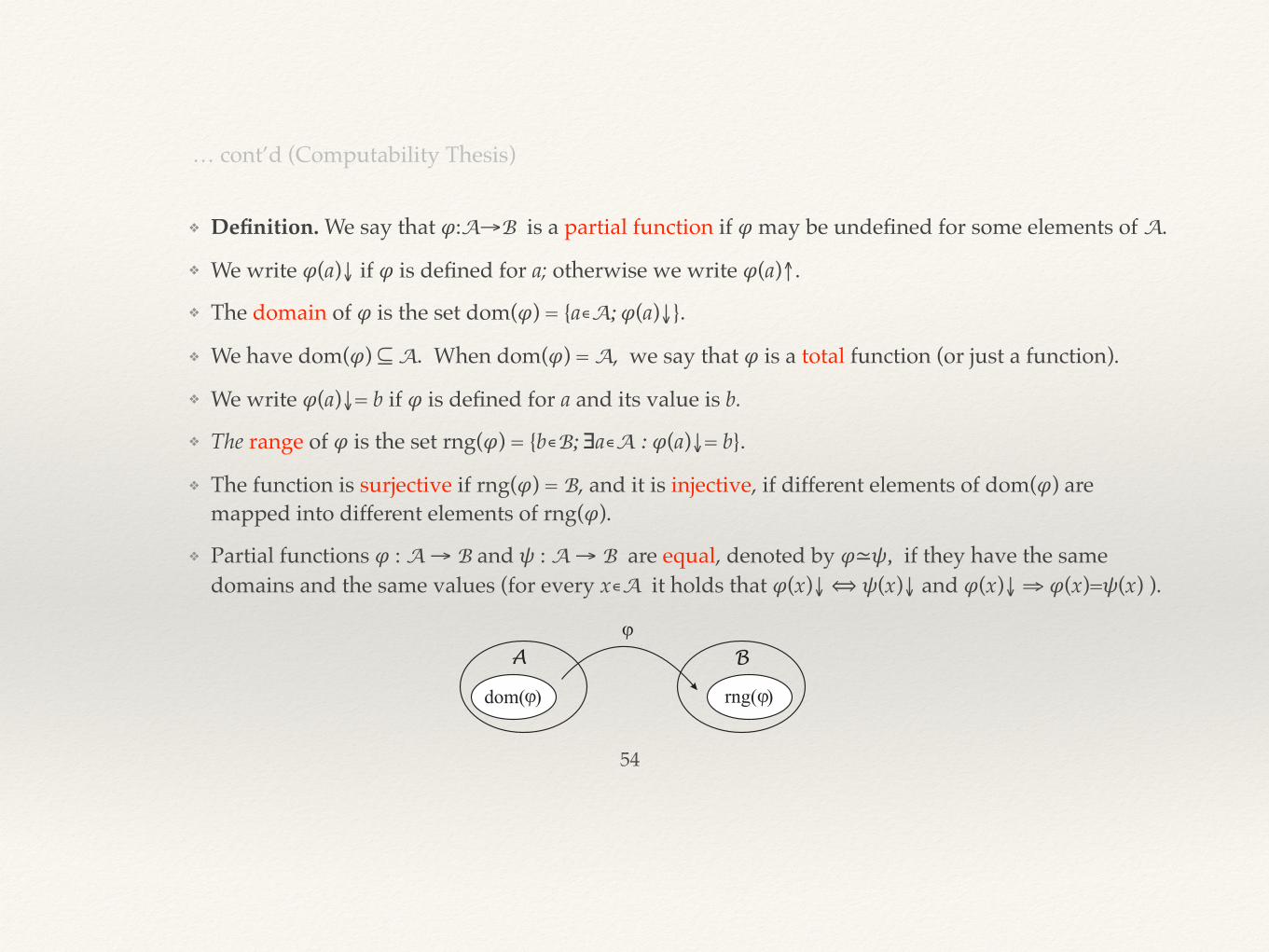
❖ Definition. We say that 𝜑:A→B is a partial function if 𝜑 may be undefined for some elements of A.

❖ We write 𝜑(a)↓ if 𝜑 is defined for a; otherwise we write 𝜑(a)↑.

❖ The domain of 𝜑 is the set dom(𝜑) = {a∊A; 𝜑(a)↓}.

❖ We have dom(𝜑) ⊆ A. When dom(𝜑) = A, we say that 𝜑 is a total function (or just a function).

❖ We write 𝜑(a)↓= b if 𝜑 is defined for a and its value is b.

❖ The range of 𝜑 is the set rng(𝜑) = {b∊B; ∃a∊A : 𝜑(a)↓= b}.

❖ The function is surjective if rng(𝜑) = B, and it is injective, if different elements of dom(𝜑) are mapped into different elements of rng(𝜑).

❖ Partial functions 𝜑 : A → B and 𝜓 : A → B are equal, denoted by 𝜑≃𝜓, if they have the same domains and the same values (for every x∊A it holds that 𝜑(x)↓ ⟺ 𝜓(x)↓ and 𝜑(x)↓ ⇒ 𝜑(x)=𝜓(x) ).


54

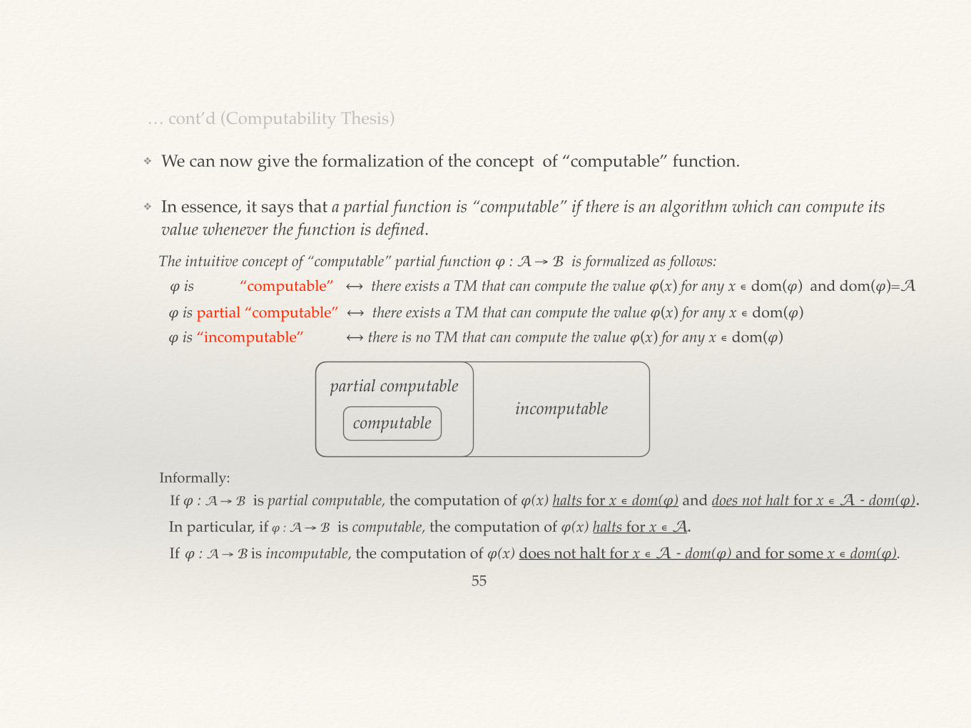
❖ We can now give the formalization of the concept of “computable” function.

❖ In essence, it says that a partial function is “computable” if there is an algorithm which can compute its value whenever the function is defined.


55

The intuitive concept of “computable” partial function 𝜑 : A → B is formalized as follows: 𝜑 is “computable” ⟷ there exists a TM that can compute the value 𝜑(x) for any x ∊ dom(𝜑) and dom(𝜑)=A

𝜑 is partial “computable” ⟷ there exists a TM that can compute the value 𝜑(x) for any x ∊ dom(𝜑) 𝜑 is “incomputable” ⟷ there is no TM that can compute the value 𝜑(x) for any x ∊ dom(𝜑)

Informally: If 𝜑 : A → B is partial computable, the computation of 𝜑(x) halts for x ∊ dom(𝜑) and does not halt for x ∊ A - dom(𝜑). In particular, if 𝜑 : A → B is computable, the computation of 𝜑(x) halts for x ∊ A.

If 𝜑 : A → B is incomputable, the computation of 𝜑(x) does not halt for x ∊ A - dom(𝜑) and for some x ∊ dom(𝜑).

partial computable

computableincomputable

Ch 6. The Turing Machine❖ The Turing machine (TM) is a model of computation that

convincingly formalized intuitive concepts of algorithm, computation, and computable function. Most researchers accepted it as the most appropriate model of computation. We will build on the TM.

❖ There is a basic variant of the TM and generalized variants.

56

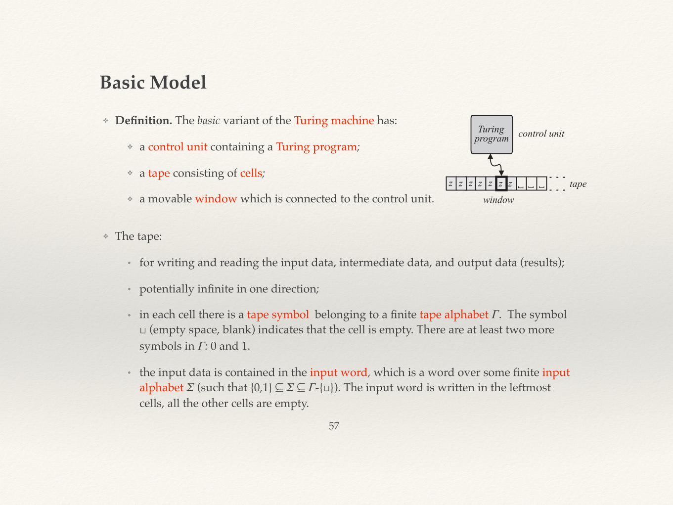
❖ Definition. The basic variant of the Turing machine has:

❖ a control unit containing a Turing program;

❖ a tape consisting of cells;

❖ a movable window which is connected to the control unit.

Basic Model

57

❖ The tape:

• for writing and reading the input data, intermediate data, and output data (results);

• potentially infinite in one direction;

• in each cell there is a tape symbol belonging to a finite tape alphabet Γ. The symbol ⊔ (empty space, blank) indicates that the cell is empty. There are at least two more symbols in Γ: 0 and 1.

• the input data is contained in the input word, which is a word over some finite input alphabet Σ (such that {0,1} ⊆ Σ ⊆ Γ-{⊔}). The input word is written in the leftmost cells, all the other cells are empty.

58

❖ The control unit:

• always in some state belonging to a finite set of states Q. The initial state is q1. Some states are final; they are in the set of final states F ⊆ Q.

• contains a program called the Turing program TP.

❖ The Turing program

• directs the whole TM;

• characteristic of a particular TM;

• a partial function δ : Q×Γ → Q×Γ×{Left, Right, Stay} called the transition function.

❖ The window:

• can only move to the neighbouring cell (Left or Right) or stays where it is (Stay);

• the control unit can read a symbol from the current cell and write a symbol to the cell.

… cont’d (Basic Model)

59

❖ Before the TM is started:

• an input word is written to the beginning of the tape;

• the window is shifted to the beginning of the tape;


❖ Then the TM operates independently, in a mechanical stepwise fashion as instructed by δ. Specifically, if the TM is in a state qi and it reads a symbol zr , then:

• if qi is a final state, then the TM halts;

• else, if δ(qi, zr)↑, then TM halts;

• else, if δ(qi, zr)↓ = (qj , zw , D), then the TM does the following:

- changes the state to qj ;

- writes zw through the window;

- moves the window to the next cell in direction D∊{Left, Right} or leaves the window where it is (D = Stay).


60

❖ Formally, a TM is a seven-tuple T = (Q, Σ, Γ, δ, q1, ⊔, F). To fix a particular TM, we fix Q,Σ,Γ,δ,F.

❖ The computation:

• Definition. Let us start a TM T on an input word w. The internal configuration of T after a finite number of computational steps is the word uqiv, where

- qi is the current state of T;

- uv are the current contents of the tape (up to (a) the rightmost non-blank symbol or (b) the symbol to the left of the window, whichever of a,b is rightmost);

- T is scanning leftmost symbol of v (in case a) and ⊔ (in case b).

• The initial configuration is q1w.

• Given an internal configuration, the next internal configuration can easily be constructed using the transition function δ.

• The computation of T on w is represented by a sequence of internal configurations starting with the initial configuration.

• Just as the computation may not halt, the sequence may also be infinite.


❖ There are several generalizations of the basic model. Each extends the basic model in some respect:

❖ Finite storage TM: The control unit can memorize several tape symbols and use them during computation.

❖ Multi-track TM: The tape is divided into several tracks, each containing its own contents.

❖ Two-way unbounded TM: The tape is potentially infinite in both directions.

❖ Multi-tape TM: There are several tapes each having its own window that is independent of other windows.

❖ Multidimensional TM: The tape is multi-dimensional.

❖ Nondeterministic TM: The transition function offers alternative transitions and the machine always chooses the “right” one.

❖ Although each of the generalizations seem to be more powerful than the basic model, it is not so.

Generalized Models

61

Each of the generalisations is equivalent to the basic model.This is because each of them can be simulated by the basic model.

❖ There are also simplifications of the basic model. Each fixes the basic model in some respect. By fixing everything to the simplest possibility we obtain:

❖ Reduced model: The parameters Σ, Γ, F in the formal definition of the Turing machine T = (Q, Σ, Γ, δ, q1, ⊔, F) are fixed as follows: Σ := {0,1}; Γ := {0,1,⊔}; F := {q2}. So, the reduced TMs are T = (Q, {0,1}, {0,1,⊔}, δ, q1, ⊔, {q2}). Since Q can be determined from δ, the reduced TMs can be specified by their δs only.

❖ Although the reduced model seems to be less powerful than the basic one, it is not so.

Reduced Models

62

The reduced model is equivalent to the basic model.This is because the basic model can be be simulated by the reduced model.

❖ If each TM were described by a characteristic natural number (index), then each TM could compute with other TMs by including their indexes into its input word. Such coding would also enable self-reference of TMs.

❖ Coding and enumeration of TMs:

❖ Let T = (Q, Σ, Γ, δ, q1, ⊔, F) be an arbitrary TM and δ(qi , zj) = (qk, zℓ, Dm) an instruction of its TP. We encode the instruction by the word K = 0i10j10k10ℓ10m, where D1 = Left, D2 = Right, and D3 = Stay.

❖ In this way, we encode each instruction of the program δ.

❖ From the codes K1, K2 ,…, Kr we construct the code of T: ⟨T⟩ = 111K111K211…11Kr111.

❖ We interpret ⟨T⟩ to be the binary code of some natural number. We call this number the index of T.

❖ Convention: Any natural number whose binary code is not of the above form is an index of the empty TM (TP of the empty TM is everywhere undefined.).

❖ Every natural number is the index of exactly one Turing machine; we can speak of i-th TM, Ti.

Universal Turing Machine

63

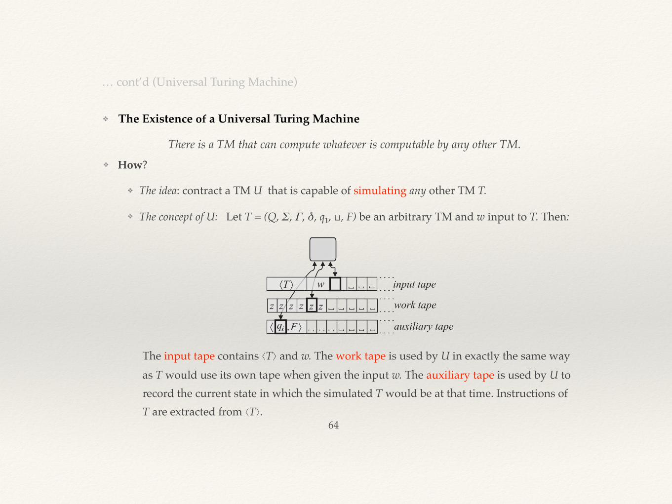
❖ The Existence of a Universal Turing Machine

64

… cont’d (Universal Turing Machine)

❖ How?

❖ The idea: contract a TM U that is capable of simulating any other TM T.

❖ The concept of U: Let T = (Q, Σ, Γ, δ, q1, ⊔, F) be an arbitrary TM and w input to T. Then:

There is a TM that can compute whatever is computable by any other TM.

The input tape contains ⟨T⟩ and w. The work tape is used by U in exactly the same way as T would use its own tape when given the input w. The auxiliary tape is used by U to record the current state in which the simulated T would be at that time. Instructions of T are extracted from ⟨T⟩.

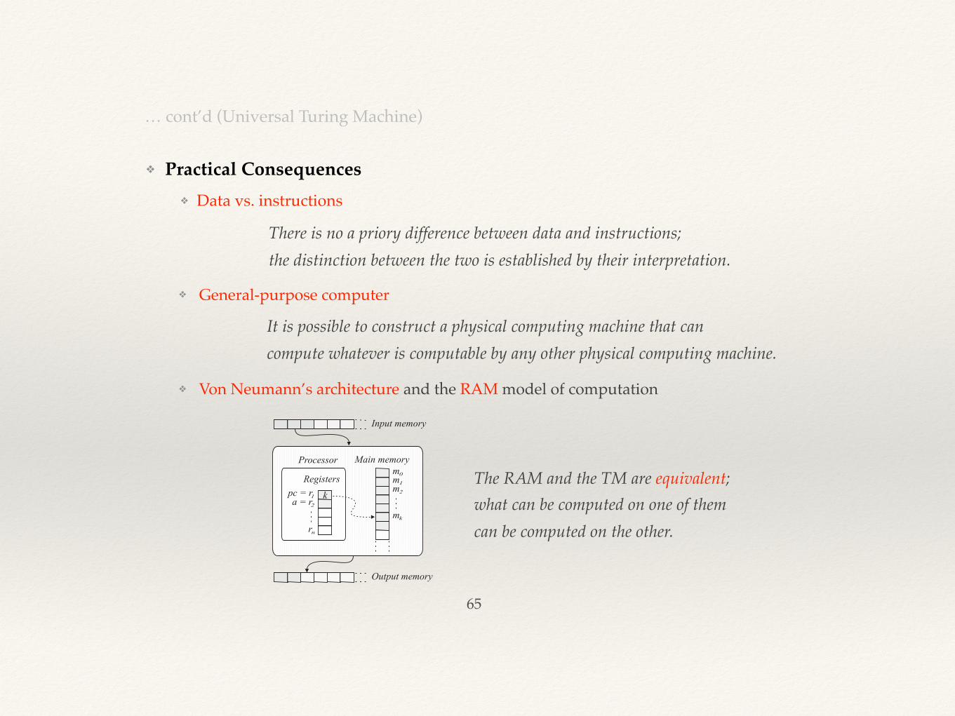
❖ Practical Consequences ❖ Data vs. instructions

65

… cont’d (Universal Turing Machine)

❖ General-purpose computer

There is no a priory difference between data and instructions; the distinction between the two is established by their interpretation.

It is possible to construct a physical computing machine that can compute whatever is computable by any other physical computing machine.

❖ Von Neumann’s architecture and the RAM model of computation

The RAM and the TM are equivalent;what can be computed on one of them can be computed on the other.

❖ There are three elementary tasks for which we can use Turing machine:

❖ Function computation: given a function 𝜑 and u1,…,uk, compute 𝜑(u1,…,uk)

❖ Set generation: given a set S, list all of its elements

❖ Set recognition: given a set S and an x, answer the question x ∈? S

Use of a Turing Machine

66

❖ Let T = (Q, Σ, Γ, δ, q1, ⊔, F) be an arbitrary TM and u1,…,uk words written in Σ. Write u1,…,uk to the tape, start T, and wait until T halts and leaves a single word in Σ on the tape. If this happens, and the resulting word is denoted by v, then we say that T has computed the value v of its k-ary proper function, 𝜓T(k), for the arguments u1,…,uk.

❖ If e is an index of T, we also denote the k-ary proper function of T by 𝜓e(k). When k is known from the context, we write just 𝜓T or 𝜓e .

❖ The interpretation of the words u1,…,uk and v is left to us. For example, they can be (encodings of) natural numbers.

67

… cont’d (Use of a Turing Machine)

Function Computation

A TM is implicitly associated, for each k ⩾ 1, with a k-ary function, called a proper function.

❖ Given a function 𝜑 : (Σ*)k → Σ*, find a TM T = (Q, Σ, Γ, δ, q1, ⊔, F) capable of computing 𝜑’s values, i.e., a T such that 𝜓T

(k) = 𝜑.

❖ Depending on how powerful, if at all, such a T can be, we distinguish between three kinds of 𝜑s.

❖ Definition. Let 𝜑 : (Σ*)k → Σ* be a function. We say that

• 𝜑 is computable if there is a TM that can compute 𝜑 anywhere on dom(𝜑) and dom(𝜑)= (Σ*)k;

• 𝜑 is partial computable if there is a TM that can compute 𝜑 anywhere on dom(𝜑);

• 𝜑 is incomputable if there is no TM that can compute 𝜑 anywhere on dom(𝜑).

68


… cont’d (Function Computation)

Instead of constructing 𝜓T(k) we often face the opposite question:

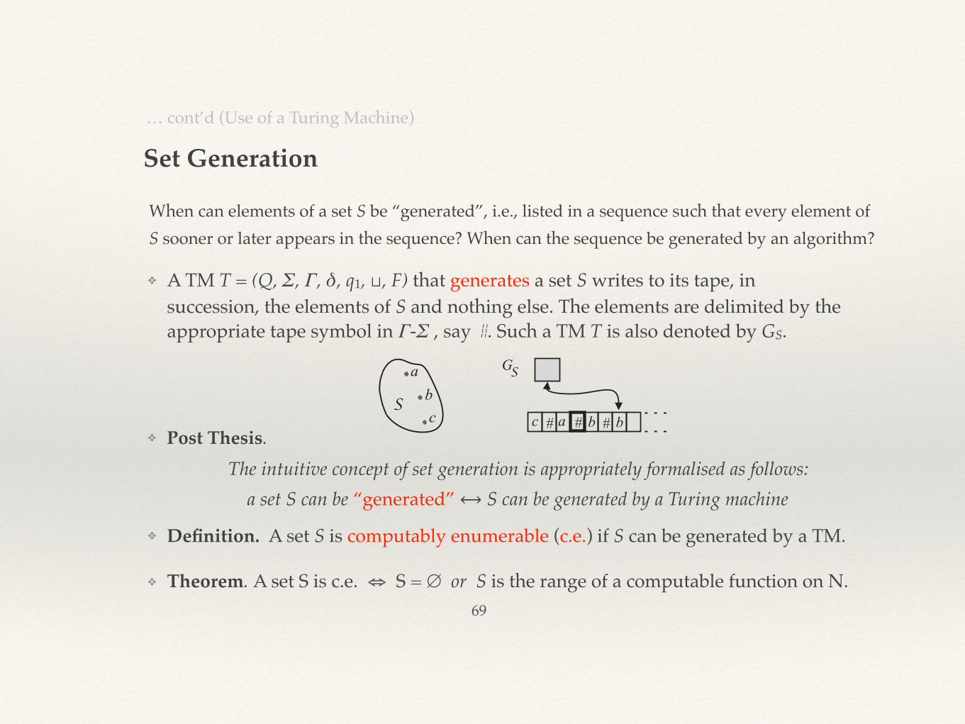
❖ A TM T = (Q, Σ, Γ, δ, q1, ⊔, F) that generates a set S writes to its tape, in succession, the elements of S and nothing else. The elements are delimited by the appropriate tape symbol in Γ-Σ , say #. Such a TM T is also denoted by GS.

69


Set Generation

When can elements of a set S be “generated”, i.e., listed in a sequence such that every element of S sooner or later appears in the sequence? When can the sequence be generated by an algorithm?

The intuitive concept of set generation is appropriately formalised as follows: a set S can be “generated” ⟷ S can be generated by a Turing machine

❖ Definition. A set S is computably enumerable (c.e.) if S can be generated by a TM.

❖ Theorem. A set S is c.e. ⇔ S = ∅ or S is the range of a computable function on N.

❖ Post Thesis.

❖ Let T = (Q, Σ, Γ, δ, q1, ⊔, F) be an arbitrary TM and w ∈ Σ*. Write w to the tape, start T, and wait until T halts. If T halts in a final state, we say that T accepts w.

❖ If T halts on w in a non-final state, we say that it rejects w; if T never halts, we say that it does not recognize w.

❖ The proper set of T is the set of all the words that T accept; it is denoted by L(T).

70


Set Recognition

A TM is implicitly associated with a set, called its proper set.

❖ Given a set S, find a TM T such that L(T) = S.

❖ The existence of such a T is connected with S’s amenability to set recognition. Informally, to completely recognise S in an environment (universe) U, is to determine which elements of U are members of S and which are not.

❖ We involve the notion of the characteristic function. The characteristic function of a set S, where S ⊆ U, is a function 𝜒s : U→{0,1} defined by 𝜒s(x)=1, if x∈S, and 𝜒s(x)=0, if x∉S. Note that 𝜒s : U→{0,1} is total.

❖ We distinguish between three kinds of sets S, based on the extent to which the values of 𝜒s can possibly be computed on U.

❖ Definition. Let U be the universe and S ⊆ U be an arbitrary set. We say that

• S is decidable in U if 𝜒s is computable function on U;

• S is semi-decidable in U if 𝜒s is computable function on S;

• S is undecidable in U if 𝜒s is incomputable function on U.

71


Instead of constructing L(T), we often face the opposite question:

… cont’d (Set Recognition)

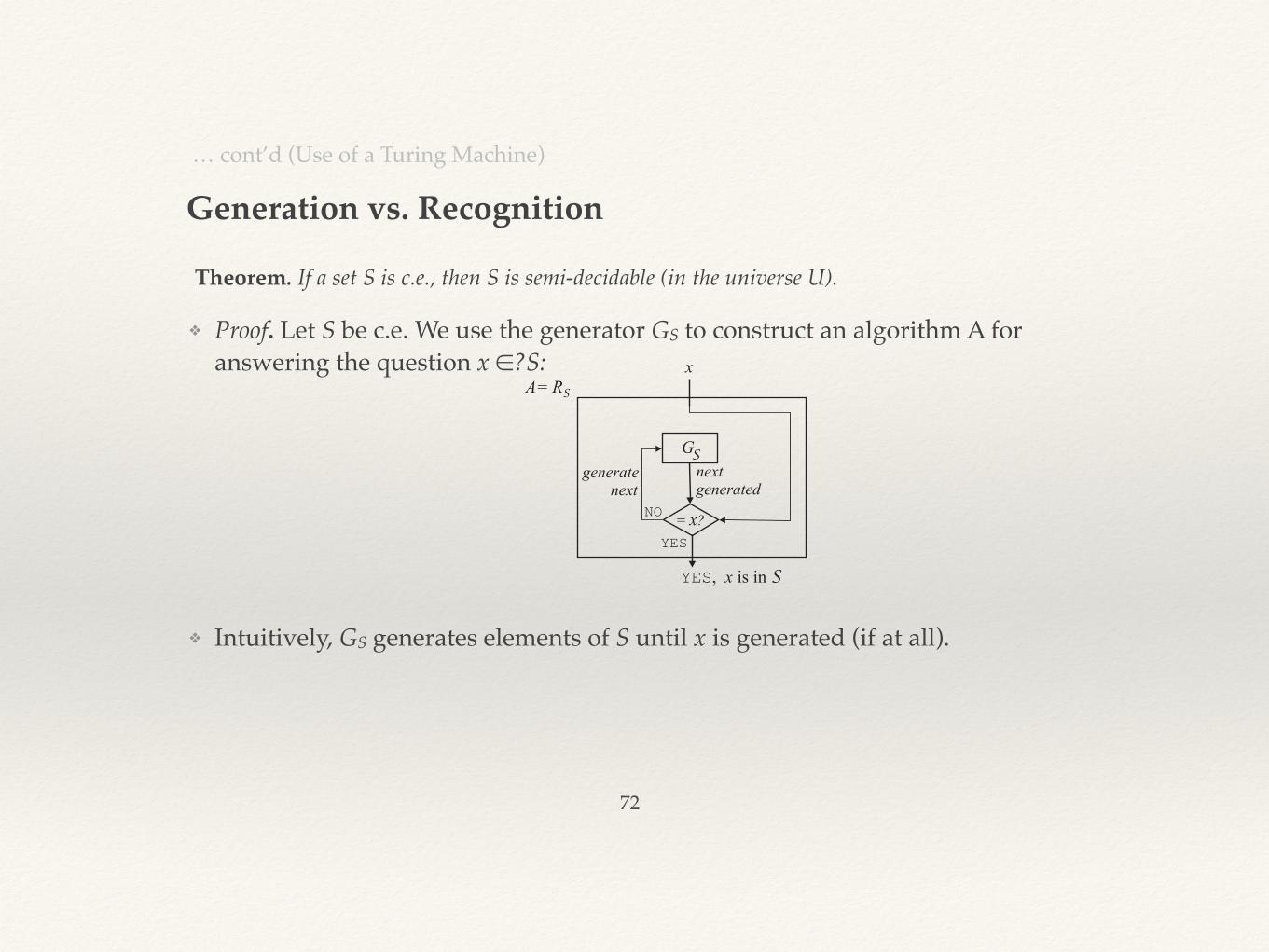
❖ Proof. Let S be c.e. We use the generator GS to construct an algorithm A for answering the question x ∈?S:

72


Generation vs. Recognition

Theorem. If a set S is c.e., then S is semi-decidable (in the universe U).

❖ Intuitively, GS generates elements of S until x is generated (if at all).

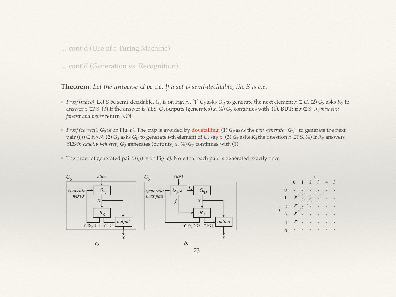
❖ Proof (naive). Let S be semi-decidable. GS is on Fig. a). (1) GS asks GU to generate the next element x ∈ U. (2) GS asks RS to answer x ∈? S. (3) If the answer is YES, GS outputs (generates) x. (4) GS continues with (1). BUT: if x ∉ S, RS may run forever and never return NO!

❖ Proof (correct). GS is on Fig. b). The trap is avoided by dovetailing. (1) GS asks the pair generator GN2 to generate the next

pair (i,j) ∈ N×N. (2) GS asks GU to generate i-th element of U, say x. (3) GS asks RS the question x ∈? S. (4) If RS answers YES in exactly j-th step, GS generates (outputs) x. (4) GS continues with (1).

❖ The order of generated pairs (i,j) is on Fig. c). Note that each pair is generated exactly once.

73


Theorem. Let the universe U be c.e. If a set is semi-decidable, the S is c.e.

… cont’d (Generation vs. Recognition)

YES, YES,

74


Recall: Σ* is the set of all the words over the alphabet Σ, and N is the set of all natural numbers.

… cont’d (Generation vs. Recognition)

Theorem. Σ* and N are c.e. sets.

Corollary. Let U = Σ* or U = N. Then: A set is semi-decidable iff S is c.e.

In what follows, we will have either U = Σ* or U = N. Why? Is this ok?

Theorem. There is a bijection f : Σ* → N.

So, when a property of sets is independent of the nature of their elements, we are allowed to choose whether to study the property using U = Σ* or U = N. The results will apply to the alternative, too. Three properties of this kind are especially interesting: the decidability, semi-decidability, and undecidability of sets. We will use the two alternatives according to the context and ease of using.

Ch 7. The First Basic Results

❖ Now, the basic notions and concepts are defined so we can start developing our theory. We will present:

❖ several theorems about c.e. sets

❖ the Padding Lemma

❖ the Parametrization (s-m-n) Theorem

❖ the Recursion (Fixed Point) Theorem

❖ Then we will present some practical consequences of the above theorems.

75

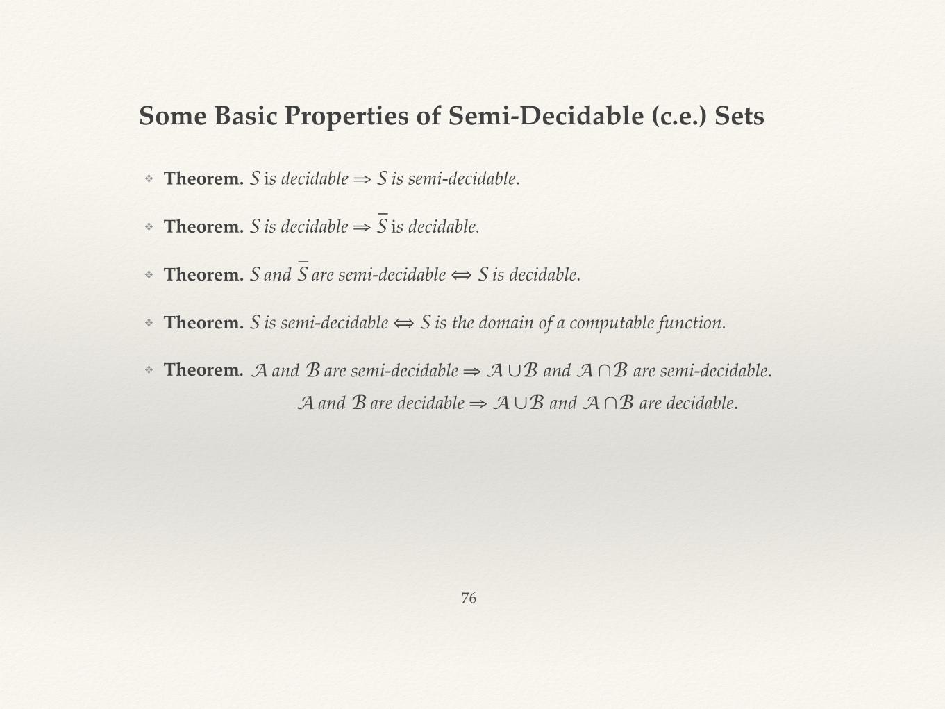
❖ Theorem. S is decidable ⇒ S is semi-decidable.

❖ Theorem. S is decidable ⇒ S is decidable.

❖ Theorem. S and S are semi-decidable ⟺ S is decidable.

❖ Theorem. S is semi-decidable ⟺ S is the domain of a computable function.

❖ Theorem.

Some Basic Properties of Semi-Decidable (c.e.) Sets

76

A and B are semi-decidable ⇒ A ∪B and A ∩B are semi-decidable. A and B are decidable ⇒ A ∪B and A ∩B are decidable.

_

_

❖ We already know: Each natural number is the index of exactly one TM. What about the other way round? Is each TM represented by exactly one index? No!

❖ A TM has many indexes. Let T be a TM and ⟨T⟩ = 111K111K211…11Kr111. We can

❖ permute the subwords K1 , K2 ,…, Kr or

❖ insert new subwords Kr+1 , Kr+2 ,… , where each of them represents a redundant instruction (that will never be executed).

Padding Lemma

77

By such permuting and padding we can construct unlimited number of new codes. Each of them describes a different yet equivalent program (i.e., it executes in the same way as T’s program). Hence, also a partial computable function has several indexes.

❖ Lemma. A partial computable function has countably infinitely many indexes. Given one of them, the others can be generated.

❖ Definition. The index set of a p.c. function 𝜑 is the set ind(𝜑) = {x ∈ N ⏐ 𝜓x ≃ 𝜑}.

❖ Let 𝜑x(y,z) be a p.c. function. Fix the variable y := p ∈ N. (We call p the parameter.) Hence, we obtain a new p.c. function of one variable, 𝜓(z) = 𝜑x(p,z). What is the index of 𝜓? The parametrization theorem states that 𝜓’s index only depends on x and p and it can be computed by a computable function.

❖ Theorem.(Parametrization) There is injective computable function s : N2 → N such that, for every x,p ∈ N, we have 𝜑x(p,z) = 𝜓s(x,p)(z).

❖ The generalization to more variables and parameters is called the s-m-n theorem.

❖ Theorem.(s-m-n) For any m,n ≧ 1 there is injective computable function smn : Nm+1 → N such that, for every x, p1, …, pm ∈ N, 𝜑x(p1, …, pm, z1, …, zn) = 𝜓s(x, p1, …, pm)(z1, …, zn).

❖ Informally: input parameters can be eliminated and, instead, integrated into the program.

Parametrization (s-m-n) Theorem

78

❖ Let f : N → N be an arbitrary computable function. Recall: f is total.

❖ We can view f as a transformation that modifies every TM Ti into Tf(i) by transforming Ti ’s program (encoded by i) into another Turing program (encoded by f(i)).

❖ In general, f(i) ≠ i, so the two programs differ. What about their proper functions 𝜓i and 𝜓f(i)? This is where the recursion theorem (also called the fixed point theorem) enters.

❖ Theorem. (Recursion) For every computable function f there is an n ∈ N such that 𝜓n ≃ 𝜓f(n). The number n can be computed from the index of the function f.

❖ Informally: if f transforms every TM, then some TM (encoded by) n is transformed into an equivalent TM (encoded by) f(n). In other words, if f modifies every TM, there is always some TM Tn for which the modified TM Tf(n) computes the same function as Tn.

❖ Such an n is called the fixed point of the function f.

❖ Theorem. A computable function has countably infinitely many fixed points.

Recursion (Fixed-Point) Theorem

79

❖ The recursion theorem and parametrization theorem allow a Turing-computable function to be defined recursively, i.e., with its own index: 𝜑n = […n…x…]. We anticipated that because Turing machine and recursive functions are equivalent models, but only the latter model explicitly exhibits recursion.

❖ During its computation, a recursively defined function 𝜑n may call itself with different actual parameters. Such a function 𝜑n can be computed on a Turing machine. How?

❖ Its Turing program 𝛿 must be able to activate itself with new actual parameters.

❖ For each activation of 𝛿, TM allocates a new activation record on its tape. The activation record contains the new actual parameters and empty field for the result of this activation (i.e. call of 𝜑n).

❖ When the result is computed, it is written into the empty field of the callee’s activation record. Next, some previously designated state, called the return state, is entered. This enables the awaiting caller to resume its execution.

❖ The caller then reads the result, deletes the callee’s activation record on the tape and continues its execution right after the call.

❖ Obviously, the machine uses its tape as a stack of activation records: when a new call of 𝜑n is made (completed), the corresponding activation record is pushed on (popped from) the stack.

❖ This mechanism is used in general-purpose computer to handle procedure calls during program execution.

Practical Consequences: Recursive Program Definition and Execution

80

Ch 8. Incomputable Problems

❖Diagonalization, combined with self-reference, made it possible to discover the first incomputable problem, i.e., a decision problem called the Halting Problem, for which there is no single algorithm capable of solving every instance of the problem.

❖After that many other incomputable problems were discovered in various fields of science.

❖ Incompatibility is a constituent part of reality.

81

❖ Decision problems. The solution of a decision problem is the answer YES or NO.

❖ Search problems. The solution of a search problem is an element of a given set such that the element has a given property.

❖ Counting problems. The solution of a counting problem is the number of elements of a given set that have a given property.

❖ Generating problems. The solution of a generating problem is a list of elements of a given set that have a given property.

Decision Problems and Other Kinds of Problems

82

In the following, we will focus on decision problems.

We define the following four kinds of computational problems:

❖ The instance d of D is obtained by replacing the variables in the definition of D with actual data.

❖ An instance d ∈ D is positive or negative if the answer to d is YES or NO, respectively.

❖ Let 𝛴 be the input alphabet of a TM. The coding function is a computable and injective function code : D → 𝛴* that transforms every instance d ∈ D into a word code(d) over 𝛴. We usually write ⟨d⟩ instead of code(d).

❖ The language of a decision problem D is the set L(D) = {⟨d⟩ ∈ 𝛴*⎟ d is a positive instance of D}.

Language of a Decision Problem

83

Obviously: An instance d of D is positive ⟺ ⟨d⟩ ∈ L(D)

Let D be a decision problem. We define the following notions:

Hence: Solving a decision problem D can be reduced to recognizing the set L(D) in 𝛴*.

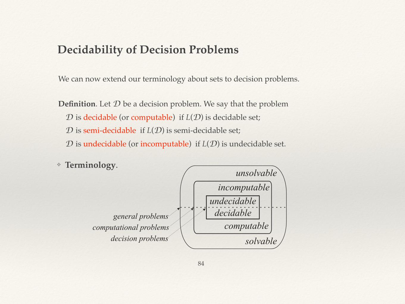
❖ Terminology.

Decidability of Decision Problems

84

We can now extend our terminology about sets to decision problems.

Definition. Let D be a decision problem. We say that the problem D is decidable (or computable) if L(D) is decidable set;D is semi-decidable if L(D) is semi-decidable set;D is undecidable (or incomputable) if L(D) is undecidable set.

Subproblems of a Decision pProblem

85

Often we encounter a decision problem that is a special version of another decision problem. Is there any connection between the decidabilities of the two problems?

Definition. A decision problem DSub is a subproblem of a decision problem DProb

if DSub is obtained from DProb by imposing additional restrictions on (some of) the variables of DProb .

Theorem. Let DSub be a subproblem of a decision problem DProb . Then: DSub is undecidable ⇒ DProb is undecidable.

There Is an Incomputable Problem - Halting Problem

86

Definition. The Halting Problem DHalt is defined by DHalt ≣ “Given a Turing machine T and word w ∈ 𝛴*, does T halt on w?”

Theorem. The Halting Problem DHalt is undecidable.

Before we go to the proof, we introduce two important sets (languages).

Definition. The universal language, denoted by Ko , is the language of the Halting Problem, that is Ko = L(DHalt) = {⟨T,w⟩⏐ T halts on w}.

Definition. The diagonal language, denoted by K , is defined by K = {⟨T,T⟩⏐T halts on ⟨T⟩}.

Observe that K is the language L(DH) of the decision problem “Given a Turing machine T, does T halt on its own code ⟨T⟩?”

87

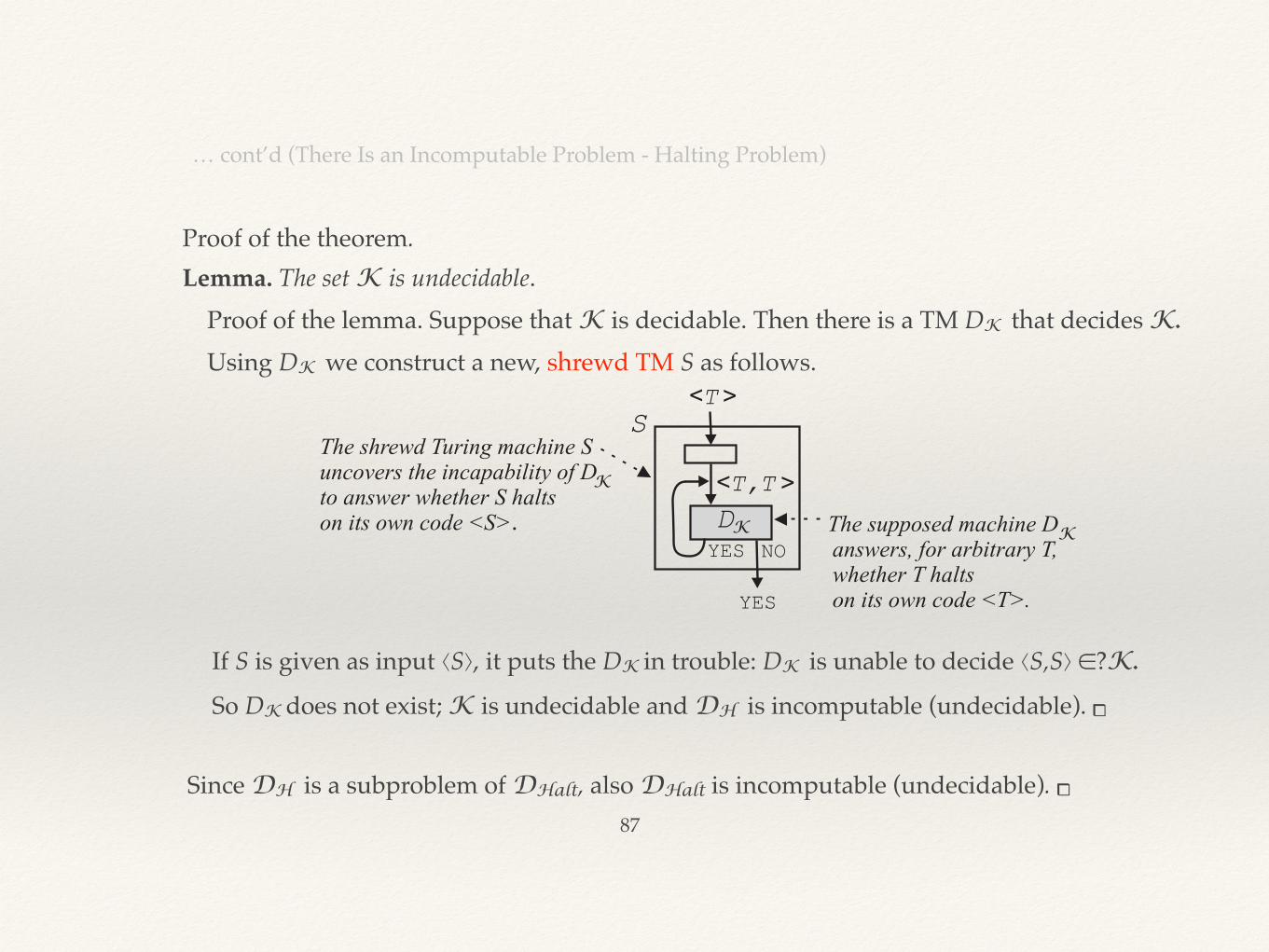
Proof of the theorem.Lemma. The set K is undecidable. Proof of the lemma. Suppose that K is decidable. Then there is a TM DK that decides K.

Using DK we construct a new, shrewd TM S as follows.

… cont’d (There Is an Incomputable Problem - Halting Problem)

If S is given as input ⟨S⟩, it puts the DK in trouble: DK is unable to decide ⟨S,S⟩ ∈?K.

So DK does not exist; K is undecidable and DH is incomputable (undecidable). ⧠

Since DH is a subproblem of DHalt, also DHalt is incomputable (undecidable). ⧠

88

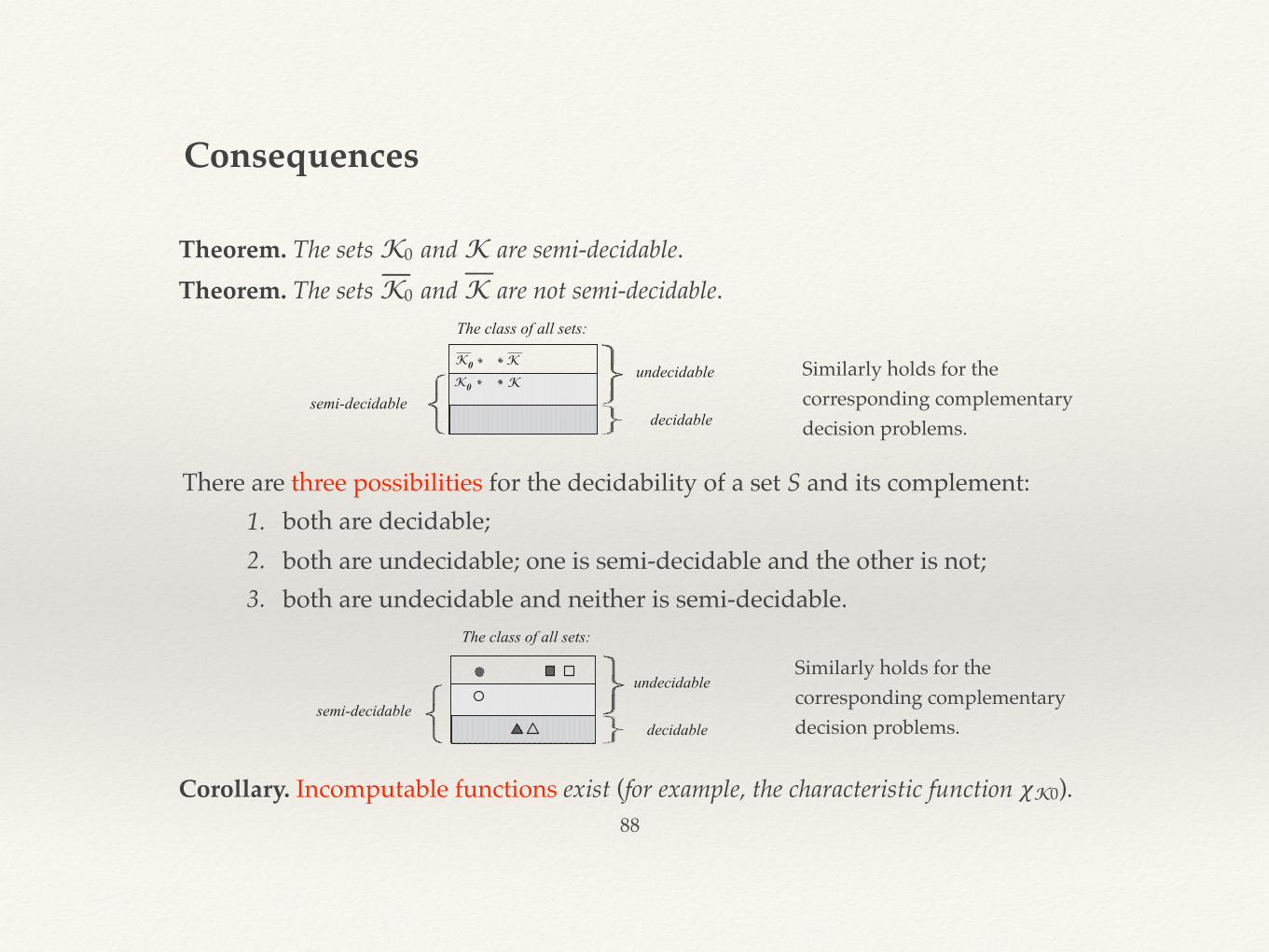
Theorem. The sets K0 and K are semi-decidable.Theorem. The sets K0 and K are not semi-decidable.

Consequences

There are three possibilities for the decidability of a set S and its complement:1. both are decidable;2. both are undecidable; one is semi-decidable and the other is not;3. both are undecidable and neither is semi-decidable.

Similarly holds for the corresponding complementary decision problems.

Similarly holds for the corresponding complementary decision problems.

Corollary. Incomputable functions exist (for example, the characteristic function 𝜒K0).

____

❖ some problems about Turing machines

❖ Post’s correspondence problem

❖ some problems about algorithms and computer programs

❖ some problems about programming languages and grammars

❖ some problems about computable functions

❖ some problems from number theory

❖ some problems from algebra

❖ some problems from analysis

❖ some problems from topology

❖ some problems from mathematical logic

❖ some problems about games

Some Other Incomputable Problems

89

There are many other incomputable problems. For example, incomputable are:

Ch 9. Methods of Proving the Incomputability

❖ Today we have at our disposal several methods of proving the undecidability of decision problems. These are:

• proving by diagonalization

• proving by reduction

• proving by Recursion Theorem

• proving by Rice’s Theorem

90

91

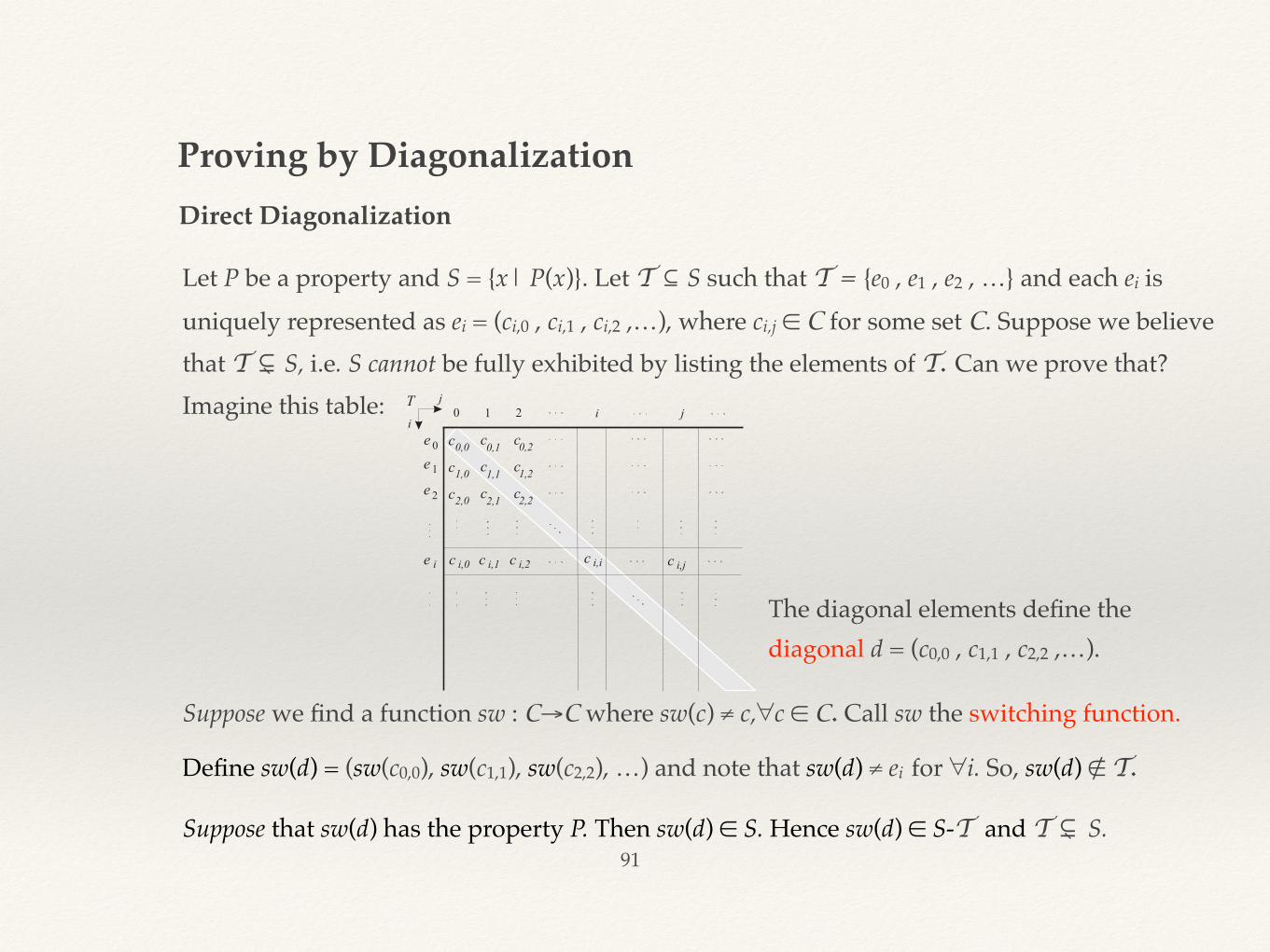
Let P be a property and S = {x| P(x)}. Let T ⊆ S such that T = {e0 , e1 , e2 , …} and each ei is uniquely represented as ei = (ci,0 , ci,1 , ci,2 ,…), where ci,j ∈ C for some set C. Suppose we believe that T ⊊ S, i.e. S cannot be fully exhibited by listing the elements of T. Can we prove that?Imagine this table:

Suppose we find a function sw : C→C where sw(c) ≠ c,∀c ∈ C. Call sw the switching function.

Define sw(d) = (sw(c0,0), sw(c1,1), sw(c2,2), …) and note that sw(d) ≠ ei for ∀i. So, sw(d) ∉ T.

Suppose that sw(d) has the property P. Then sw(d) ∈ S. Hence sw(d) ∈ S-T and T ⊊ S.

The diagonal elements define the diagonal d = (c0,0 , c1,1 , c2,2 ,…).

Direct Diagonalization

Proving by Diagonalization

92

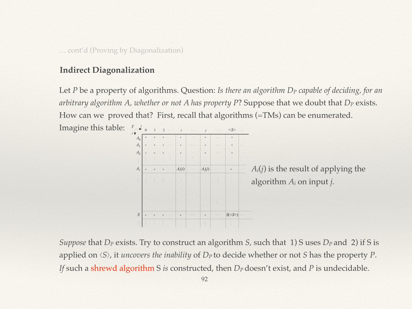
Let P be a property of algorithms. Question: Is there an algorithm DP capable of deciding, for an arbitrary algorithm A, whether or not A has property P? Suppose that we doubt that DP exists. How can we proved that? First, recall that algorithms (=TMs) can be enumerated.Imagine this table:

Suppose that DP exists. Try to construct an algorithm S, such that 1) S uses DP and 2) if S is applied on ⟨S⟩, it uncovers the inability of DP to decide whether or not S has the property P. If such a shrewd algorithm S is constructed, then DP doesn’t exist, and P is undecidable.

Ai(j) is the result of applying the algorithm Ai on input j.

Indirect Diagonalization

… cont’d (Proving by Diagonalization)

93

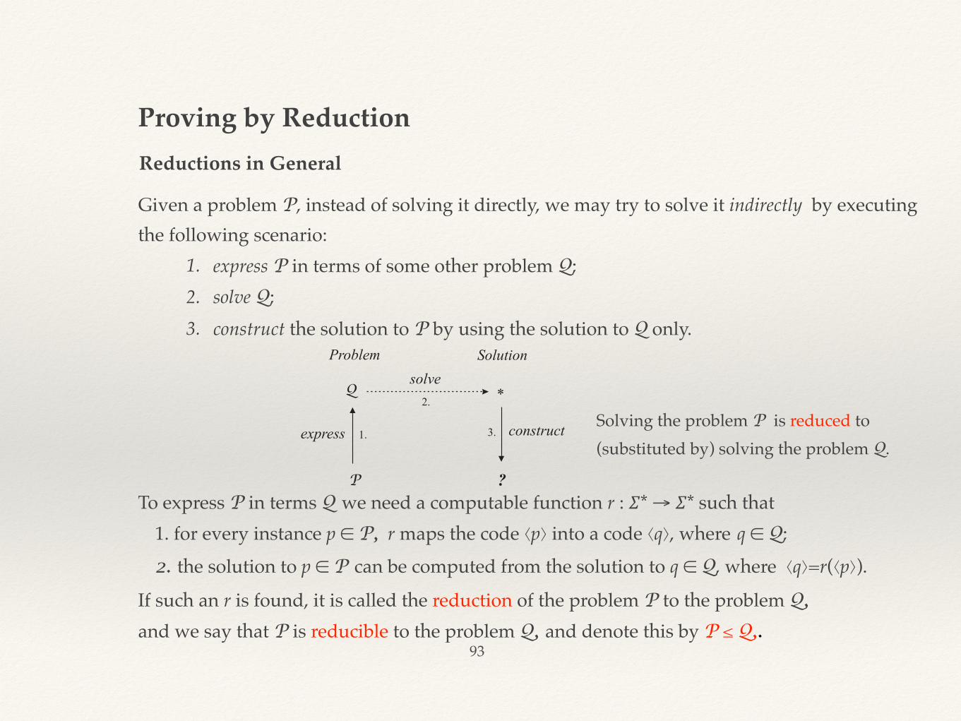
Given a problem P, instead of solving it directly, we may try to solve it indirectly by executing the following scenario:

1. express P in terms of some other problem Q;2. solve Q;3. construct the solution to P by using the solution to Q only.

To express P in terms Q we need a computable function r : 𝛴* → 𝛴* such that 1. for every instance p ∈ P, r maps the code ⟨p⟩ into a code ⟨q⟩, where q ∈ Q; 2. the solution to p ∈ P can be computed from the solution to q ∈ Q, where ⟨q⟩=r(⟨p⟩).

If such an r is found, it is called the reduction of the problem P to the problem Q,

and we say that P is reducible to the problem Q, and denote this by P ≤ Q,.

Solving the problem P is reduced to (substituted by) solving the problem Q.

Reductions in General

Proving by Reduction

94

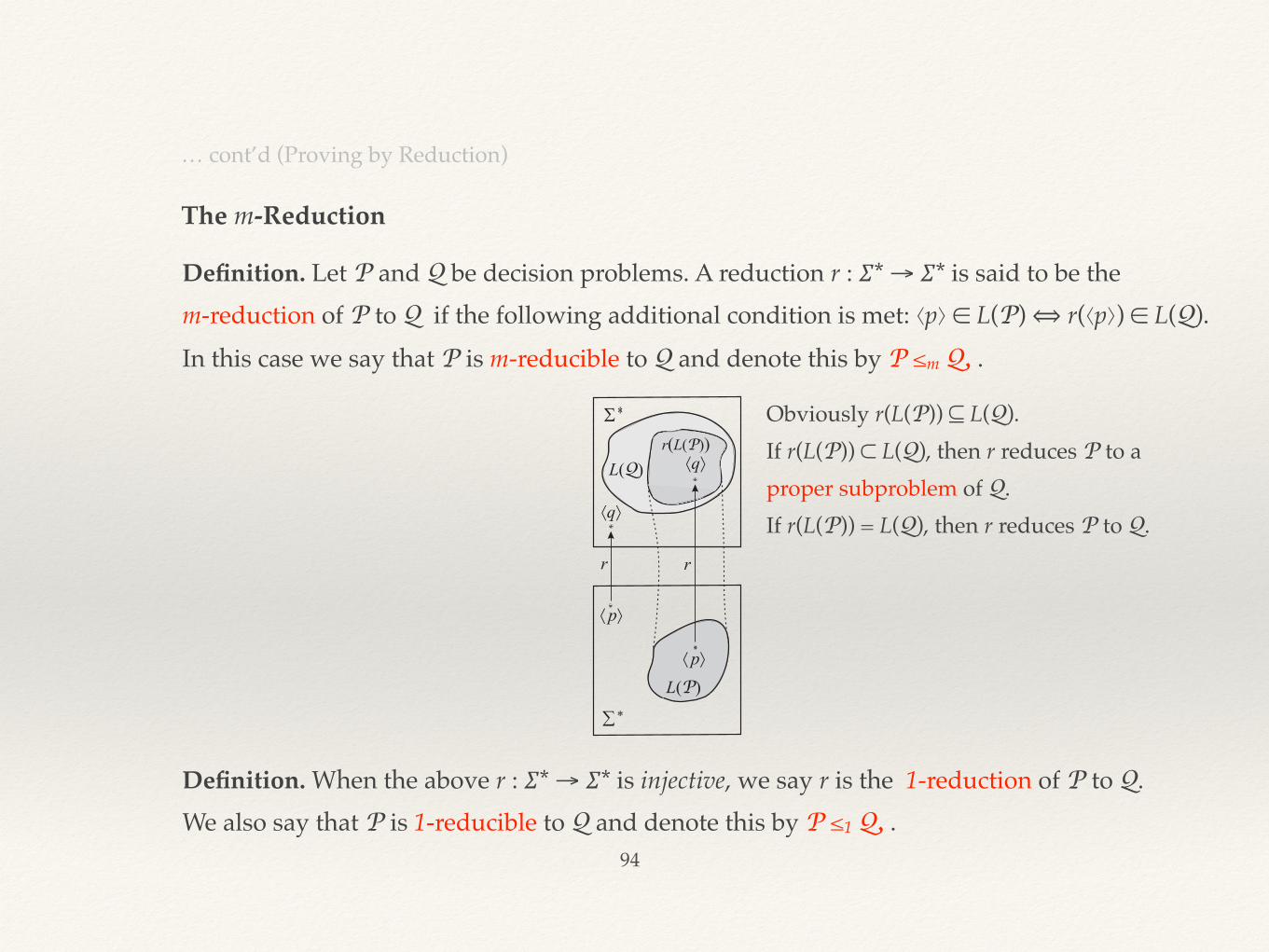
Definition. Let P and Q be decision problems. A reduction r : 𝛴* → 𝛴* is said to be the m-reduction of P to Q if the following additional condition is met: ⟨p⟩ ∈ L(P) ⟺ r(⟨p⟩) ∈ L(Q).In this case we say that P is m-reducible to Q and denote this by P ≤m Q, .

Obviously r(L(P)) ⊆ L(Q). If r(L(P)) ⊂ L(Q), then r reduces P to a proper subproblem of Q. If r(L(P)) = L(Q), then r reduces P to Q.

The m-Reduction

… cont’d (Proving by Reduction)

Definition. When the above r : 𝛴* → 𝛴* is injective, we say r is the 1-reduction of P to Q.We also say that P is 1-reducible to Q and denote this by P ≤1 Q, .

95

Theorem. Let P and Q be decision problems. Then: a) P ≤m Q, ⋀ Q, is decidable ⇒ P is decidable

b) P ≤m Q, ⋀ Q, is semi-decidable ⇒ P is semi-decidable

Corollary. Let U and Q be decision problems. Then: U is undecidable ⋀ U ≤m Q, ⇒ Q is undecidable

This is the backbone of the following method.Method. The undecidability of a decision problem Q can be proved as follows:

1. Select an undecidable problem Q

2. Prove that U ≤m Q

3. Conclude: Q is undecidable

… cont’d (Proving by Reduction)

… cont’d (The m-Reduction)

96

Recall the Fixed-Point Theorem: Every computable function has a fixed point.

This reveals the following method for proving the incompatibility of functions:

Method. Let g be a function with no fixed point. Then, g is not computable, i.e., it is not total, or it is incomputable, or both. If we prove that g is total, then g must be incomputable.

We can develop this into a method for proving the undecidability of decision problems.

Method. Undecidability of a decision problem D can be proved as follows:1. Suppose that D is a decidable problem2. Construct a computable function g using the characteristic function 𝜒L(D)

3. Prove that g has no fixed point4. This is a contradiction with the Fixed-Point Theorem5. Conclude that D is undecidable

Proving by the Recursion Theorem

97

Definitions. • Let P be a property sensible for functions. We say that P is intrinsic property of

functions if functions are viewed only as mappings from one set to another; that is, P is insensitive to the machine, algorithm, and program, that are used to compute function values.

• Let P be a property intrinsic to functions, and 𝜑 an arbitrary p.c. function. Define the following decision problem: DP = “Does a p.c. function 𝜑 have the property P?’’ We say that P is a decidable property if DP is a decidable problem.

• We say that an intrinsic property of functions is trivial if either every p.c. function has the property P or no p.c. function has the property P.

Theorem. Let P be an arbitrary intrinsic property of p.c. functions. Then: P is a decidable property ⟺ P is trivial

Proving by the Rice’s Theorem

Rice’s Theorem for Functions

98

Based on this, we obtain the following method.

Method. Given a property P, the undecidability of the decision problem DP = “Does a p.c. function 𝜑 have the property P?’’ can be proved as follows:

1. Show that P meets the following conditions a. P is a property sensible for functions b. P is insensitive to the machine, algorithm, or program used to compute 𝜑

2. If P fulfills the above conditons, then show that P is non-trivial. To do this, c. find a p.c. function that has the property P d. find a p.c. function that does not have the property P

If all the steps are successful, then the problem DP is undecidable.

… cont’d (Proving by the Rice’s Theorem)

… cont’d (Rice’s Theorem for Functions)

99

Definitions. • Let P be an intrinsic property of p.c. functions. Define F to be the class of all the p.c.

functions having the property P; that is, F = {𝜓|𝜓 has the property P}. • The decision problem DP can be now rewritten as DP = “𝜑 ∈ ? F’’’.• Define ind(F) = ∪𝜓∈F ind(𝜓). In other words, ind(F) is the set of all of the indexes of

all Turing Machines that compute any of the functions F.• The decision problem DP can now be rewritten as DP = “x ∈ ? ind(F’)’’.

So, DP is a decidable problem iff ind(F’) is a decidable set. But, when is ind(F’) decidable?

Theorem. Let F be an arbitrary set of p.c. functions. Then:

ind(F’) is a decidable set ⟺ ind(F’) is either Ø or ℕ

Rice’s Theorem for Index Sets


100

Definitions. • Let R be a property sensible sets. We say that R is intrinsic property of sets if it is

independent of the way of recognizing the sets; that is, R is insensitive to the machine, algorithm, and program, that are used to recognize the sets.

• Let R be a property intrinsic to sets, and X an arbitrary c.e. set. Define the following decision problem: DR = “Does a c.e. set X have the property R?’’ We say that R is a decidable property if DR is a decidable problem.

• We say that an intrinsic property of c.e. sets is trivial if it holds for all c.e. sets or for none.

Theorem. Let R be an arbitrary intrinsic property of c.e. sets. Then: R is a decidable property ⟺ R is trivial

Rice’s Theorem for Sets


101

Based on this, we obtain the following method.

Method. Given a property R, the undecidability of the decision problem DR = “Does a c.e. set X have the property R?’’ can be proved as follows:

1. Show that R meets the following conditions a. R is a property sensible for setsb. R is insensitive to the machine, algorithm, or program used to recognise X

2. If R fulfills the above conditons, then show that R is non-trivial. To do this, c. find a c.e. set that has the property Rd. find a c.e. set that does not have the property R

If all the steps are successful, then the problem DR is undecidable.


… cont’d (Rice’s Theorem for Sets)

Part III. RELATIVE COMPUTABILITY ❖ Ch 10 Computation with external help

❖ Ch 11 Degrees of unsolvability

❖ Ch 12 The Turing hierarchy of unsolvability

❖ Ch 13 The class D of degrees of unsolvability

❖ Ch 14 C.E. degrees and the priority method

❖ Ch 15 The arithmetical hierarchy

102

Ch 10. Computation With External Help

❖ What if an unsolvable decision problem, for example the Halting Problem, were somehow made solvable with some hypothetical procedure?

❖ We must assume that the hypothetical procedure would not be the ordinary Turing machine; otherwise, our theory would become inconsistent.

❖ The question can be explored by introducing the oracle Turing machine.

❖ Such a machine was conceived by Alan Turing and further developed by Emil Post.

103

104

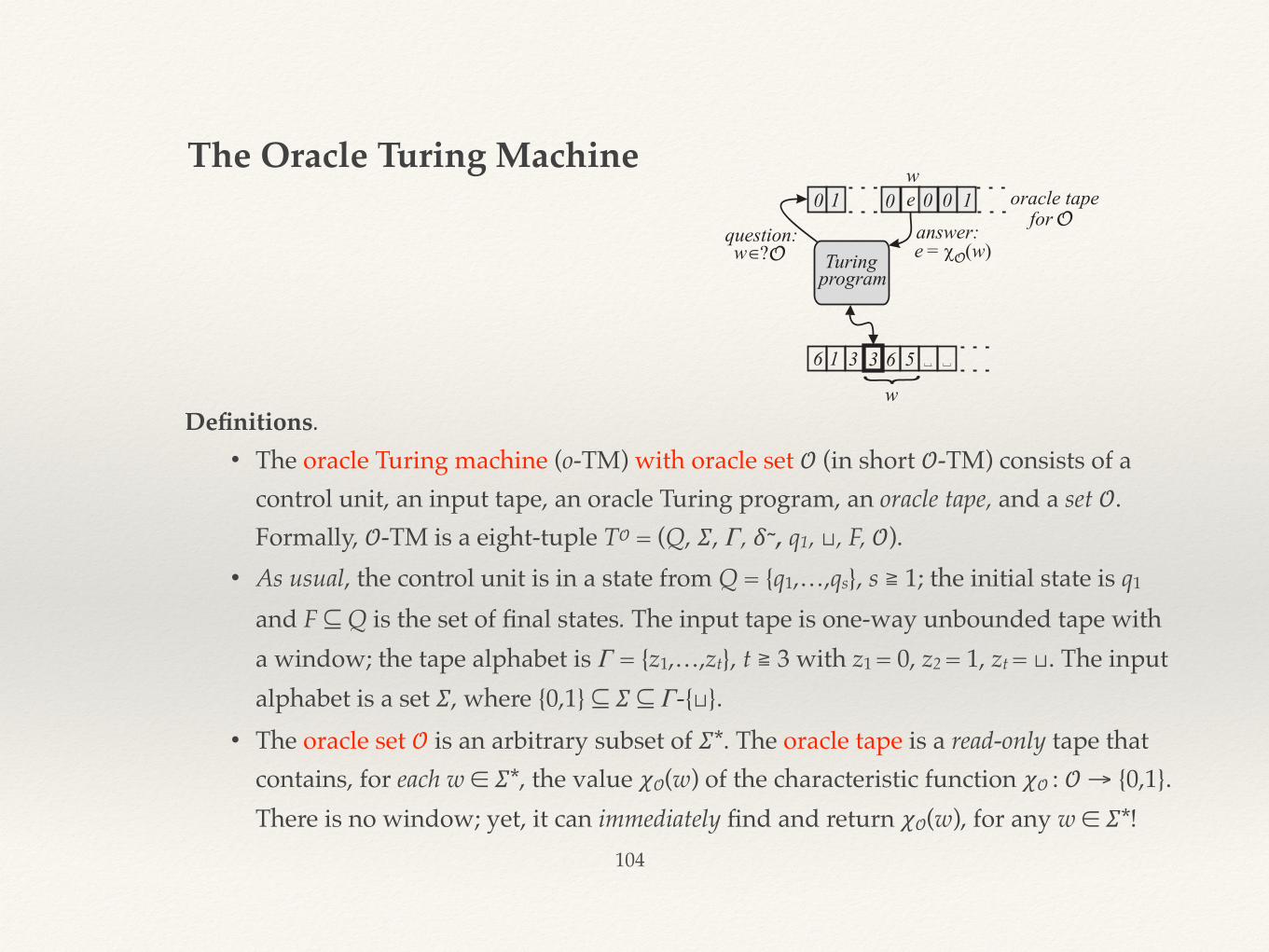
Definitions. • The oracle Turing machine (o-TM) with oracle set 𝒪 (in short 𝒪-TM) consists of a

control unit, an input tape, an oracle Turing program, an oracle tape, and a set 𝒪. Formally, 𝒪-TM is a eight-tuple T𝒪 = (Q, 𝛴, Γ, 𝛿~, q1, ⊔, F, 𝒪).

• As usual, the control unit is in a state from Q = {q1,…,qs}, s ≧ 1; the initial state is q1 and F ⊆ Q is the set of final states. The input tape is one-way unbounded tape with a window; the tape alphabet is Γ = {z1,…,zt}, t ≧ 3 with z1 = 0, z2 = 1, zt = ⊔. The input alphabet is a set 𝛴, where {0,1} ⊆ 𝛴 ⊆ Γ-{⊔}.

• The oracle set 𝒪 is an arbitrary subset of 𝛴*. The oracle tape is a read-only tape that contains, for each w ∈ 𝛴*, the value 𝜒𝒪(w) of the characteristic function 𝜒𝒪 : 𝒪 → {0,1}. There is no window; yet, it can immediately find and return 𝜒𝒪(w), for any w ∈ 𝛴*!

The Oracle Turing Machine

105

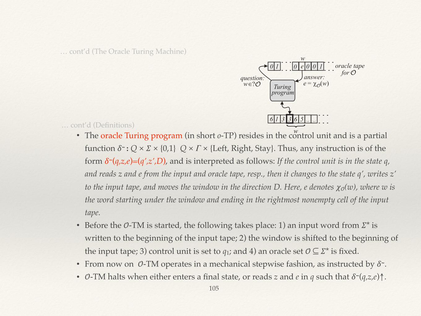
… cont’d (Definitions)• The oracle Turing program (in short o-TP) resides in the control unit and is a partial

function 𝛿~ : Q × 𝛴 × {0,1} Q × Γ × {Left, Right, Stay}. Thus, any instruction is of the form 𝛿~(q,z,e)=(q’,z’,D), and is interpreted as follows: If the control unit is in the state q, and reads z and e from the input and oracle tape, resp., then it changes to the state q’, writes z’ to the input tape, and moves the window in the direction D. Here, e denotes 𝜒𝒪(w), where w is the word starting under the window and ending in the rightmost nonempty cell of the input tape.

• Before the 𝒪-TM is started, the following takes place: 1) an input word from 𝛴* is written to the beginning of the input tape; 2) the window is shifted to the beginning of the input tape; 3) control unit is set to q1; and 4) an oracle set 𝒪 ⊆ 𝛴* is fixed.

• From now on 𝒪-TM operates in a mechanical stepwise fashion, as instructed by 𝛿~. • 𝒪-TM halts when either enters a final state, or reads z and e in q such that 𝛿~(q,z,e)↑.

… cont’d (The Oracle Turing Machine)

106

Properties: • Oracle Turing programs 𝛿~ are not affected by changes in 𝒪. • During the execution, oracle Turing programs 𝛿~ can ignore 𝒪.

Theorem. Oracle computation is a generalization of ordinary computation.

Some Basic Properties of o-TMs

❖ Coding

❖ Let T𝒪 = (Q, Σ, Γ, δ, q1, ⊔, F, 𝒪) be an arbitrary 𝒪-TM and δ~(qi , zj , e) = (qk, zℓ, Dm) an instruction of its o-TP. We encode the instruction by the word K = 0i10j10e10k10ℓ10m, where D1 = Left, D2 = Right, and D3 = Stay. In this way, we encode each instruction of the oracle program δ~.

❖ From the codes K1,…, Kr we construct the code of δ~ as follows: ⟨δ~⟩ = 111K111K211…11Kr111.

This is also the code of T𝒪, i.e. ⟨T𝒪⟩ = ⟨δ~⟩. (Note that ⟨T𝒪⟩ is independent of the particular 𝒪.)

Coding and Enumeration of o-TMs

107

❖ Enumeration

❖ We interpret ⟨T𝒪⟩ to be the binary code of some natural number, called the index of T𝒪.

❖ Convention: Any natural number whose binary code is not of the above form is an index of the empty 𝒪-TM (its o-TP is everywhere undefined).

❖ Every natural number is the index of exactly one o-TM (and 𝒪-TM); we can speak of i-th 𝒪-TM, T𝒪i.

Computation with Oracles

108

Generalization of Classical Definitions

Function Computation

❖ Definition. Let 𝒪 ⊆ 𝛴*, k ⩾ 1, and 𝜑 ⩾: (Σ*)k → Σ* a function. We say that

• 𝜑 is 𝒪-computable if there is an 𝒪-TM that can compute 𝜑 anywhere on dom(𝜑) and dom(𝜑)= (Σ*)k;

• 𝜑 is partial 𝒪-computable (or 𝒪-p.c.) if there is an 𝒪-TM that can compute 𝜑 anywhere on dom(𝜑);

• 𝜑 is 𝒪-incomputable if there is no 𝒪-TM that can compute 𝜑 anywhere on dom(𝜑).

❖ Definition. Given any 𝒪 ⊆ 𝛴* , n ⩾ 0, and k ⩾ 1, the oracle Turing machine T𝒪n computes a function 𝛹𝒪,(k)

x : (Σ*)k → Σ* called the k-ary proper functional of T𝒪n . When k is understood,

we omit it.

109

Set Recognition

❖ Definition. Let 𝒪 ⊆ 𝛴* be an oracle set. For an arbitrary S ⊆ 𝛴* we say that

• S is 𝒪-decidable (or 𝒪-computable) in 𝛴* if 𝜒s is 𝒪-computable function on 𝛴*;

• S is 𝒪-semi-decidable (or 𝒪-c.e.) in 𝛴* if 𝜒s is 𝒪-computable function on S;

• S is 𝒪-undecidable (or 𝒪-incomputable) in 𝛴* if 𝜒s is 𝒪-incomputable function on 𝛴*.

… cont’d (Computation with Oracles)

… cont’d (Generalization of Classical Definitions

110

Index Set

❖ Lemma.(Generalized Padding Lemma) An 𝒪-p.c. function has countably infinitely many indexes. Given one of them, the others can be generated.

… cont’d (Computation with Oracles)

… cont’d (Generalization of Classical Definitions

❖ Definition (Index set of 𝒪-p.c. function). The index set of an 𝒪-p.c. function 𝜑 is the set ind𝒪(𝜑) = {x ∈ ℕ|𝛹x𝒪 ⋍ 𝜑}.

111

Convention.

From now on ℕ will be the universe.

From now on we will focus on single-argument functions.

Other Ways to Make External Help Available

112

❖ Kleene introduced external help to partial recursive (p.r.) functions. Given 𝒪 ⊆ ℕ, he added the characteristic function 𝜒𝒪 to the set {ζ, 𝜋i

k, 𝜎}. Any function that can be constructed by these initial functions by finite number of applications of the rules of construction (i.e. composition, primitive recursion, 𝜇-operation) is called p.r. relative to 𝒪.

❖ Post introduced external help into his canonical systems by hypothetically adding primitive assertions expressing the (non)membership in 𝒪 .

❖ Davis proved the equivalence of Kleene’s and Post’s approaches.

❖ Based on this and following the Computability Thesis the following thesis was proposed:

Basic intuitive concepts of computing with external help are appropriately formalized as follows: “algorithm with external help” ⟷ oracle Turing program “computation with external help” ⟷ execution of an oracle TP on o-TM function “computable with external help” ⟷ 𝒪-p.c. functionInstead of the o-TM we can use any other equivalent model.

Relative Computability Thesis

Ch 11. Degrees of Unsolvability

❖ We saw that there exist solvable and unsolvable computational problems.

❖ So, it makes sense to talk about the “degree of unsolvability.”

❖ But, our understanding of the notion “degree of unsolvability” is just intuitive.

❖ Now, we want to formalize it.

113

114

Definition: (Turing Reduction) Let A, B ⊆ ℕ be arbitrary sets. We say that A is Turing

reducible (in short, T-reducible) to B, if A is B-decidable. We denote this by A ≤T B,

which reads “If B is decidable, then also A is decidable.” The relation ≤T is called the Turing reduction (in short, T-reduction).

Let P and Q be decision problems and L(P) and L(Q) their languages. We say that the

problem P is reducible to the problem Q, (and denote this by P ≤T Q) if L(P) ≤T L(Q).

Turing Reduction

115

… cont’d (Turing Reduction)

Basic Properties of the Turing Reduction

Theorem. Let A be a decidable set. Then A ≤T B for arbitrary set B.

Theorem. For every set S it holds that S ≤T S.

Theorem. If two sets are related by ≤m , then they are also related by ≤T.

Theorem. If two sets are related by ≤T , they may not be related by ≤m.

Theorem. For arbitrary sets A ,B it holds: A ≤T B ⋀ B is decidable ⇒ A is decidable

Corollary. For arbitrary sets A ,B it holds: A is undecidable ⋀ A ≤T B ⇒ B is undecidable

Theorem. Turing reduction ≤T is a reflexive and transitive relation.

—

116


Turing Degrees

Definition. Let A, B ⊆ ℕ be arbitrary sets. We say that A is Turing-equivalent (in short,

T-equivalent) to B, if A ≤T B ⋀ B ≤T A . We denote this by A ≣T B, and read “If one of

A, B were decidable, also the other would be decidable.” The relation ≣T is called the Turing equivalence (in short, T-equivalence).

Theorem. For every set S it holds that S ≣T S.

Definition. A Turing degree (in short, T-degree) of a set S, denoted by deg(S), is the

equivalence class {X ∈ 2ℕ| X ≣T S}.

Formalization. The intuitive notion of the degree of unsolvability is formalized by “degree of unsolvability” ⟷ Turing degreeTheorem. There exist at least two T-degrees:

deg(Ø) = {X ∈ 2ℕ| X ≣T Ø } and

deg(K) = {X ∈ 2ℕ| X ≣T K }

—

117


The Relation <

Definition. Let deg(A) and deg(B) be arbitrary T-degrees. Then deg(A) is lower than deg(B),

denoted by deg(A) < deg(B), if A <T B (i.e. A ≤T B ⋀ A ≢T B).

Theorem. The relation <T is irreflexive.

Since Ø <T K, we find that deg(Ø) < deg(K).

So, the degree of undecidability of decidable decision problems is lower than the degree of unsolvability of undecidable decision problems T-equivalent to the Halting Problem.

But we have intuitively anticipated this!

Nevertheless, this formalization will enable us to discover in the next chapter a surprising fact that there are many more other degrees of unsolvability!

Ch 12. The Turing hierarchy of unsolvability ❖ At this point we only know of two degrees of unsolvability: deg(Ø) and

deg(K).

❖ We will now prove that there are infinitely many other degrees of unsolvability.

❖ To prove this we will introduce the Turing jump operator.

118

119

Recall: The Halting Problem is the question “Does T halt on input ⟨T⟩?”

and its language is K = {⟨T⟩|T halts on input ⟨T⟩} = {x|Tx halts on input x} = {x|𝛹x(x)↓}.

Let S be an arbitrary set. Let us adapt the Halting Problem for oracle Turing machines TS: “Does TS halt on input ⟨TS⟩?”

and define, in the similar fashion, its language as KS = {⟨TS⟩|TS halts on input ⟨TS⟩} = {x|TxS halts on input x} = {x|𝛹xS(x)↓}.

Definition: The Turing jump of a set S is the set KS defined by KS = {x| 𝛹xS(x)↓}. The set KS we also denote by S’.

The Turing Jump

120

… cont’d (The Turing Jump)

Properties of the Turing Jump of a Set

Lemma. A is S-c.e. ⟹ A is S’-decidable

Theorem. Let S be and arbitrary set. Then S ≤T S’.

Theorem. Let S be and arbitrary set. Then:

a) S’ is S-undecidable (i.e., S’ ≰T S’)

b) S’ is S-c.e.

Corollary. Let S be and arbitrary set. Then deg(S) < deg(S’).

By taking S := K in the corollary, we obtain deg(K) < deg(K’).

We have discovered that there is a T-degree that is higher than deg(K).

Hence, there exist decision problems that are more difficult than the Halting Problem.

121


Hierarchies of T-Degrees

Definition: The nth Turing jump of the set S is the set S(n), which is inductively defined as follows: S(n) = S, if n = 0;

S(n) = (S(n-1))’, if n ⩾ 1.

Theorem. Let S be and arbitrary set. Then:

a) S(n) <T S(n+1)

b) S(n+1) is S(n)-c.e.

c) deg(S(n)) < deg(S(n+1)).

For every degree of unsolvability there is a higher degree of unsolvability. For every decision

problem, even undecidable one, there is a more difficult decision problem. There is no most

difficult decision problem.

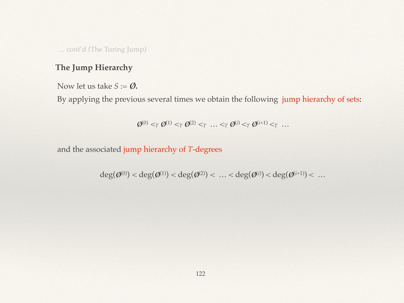
122


The Jump Hierarchy

Now let us take S := Ø. By applying the previous several times we obtain the following jump hierarchy of sets:

Ø(0) <T Ø(1) <T Ø(2) <T … <T Ø(i) <T Ø(i+1) <T …

and the associated jump hierarchy of T-degrees

deg(Ø(0)) < deg(Ø(1)) < deg(Ø(2)) < … < deg(Ø(i)) < deg(Ø(i+1)) < …

Ch 13. The Class D of Degrees of Unsolvability

❖ We will now view the collection of T-degrees as a mathematical structure D endowed with the relation < and the function ’.

❖ This view will simplify our expression and the investigation of the properties of T-degrees.

123

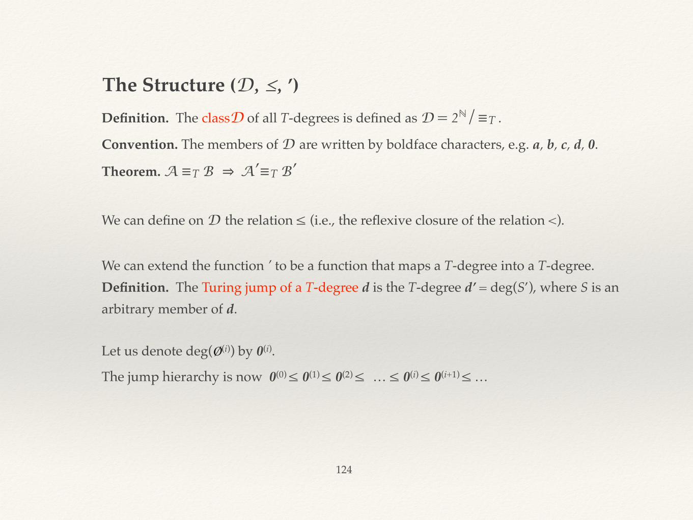
124

Definition. The classD of all T-degrees is defined as D = 2ℕ/≣T .

Convention. The members of D are written by boldface characters, e.g. a, b, c, d, 0.

Theorem. A ≣T B ⇒A’≣T B’

We can define on D the relation ≤ (i.e., the reflexive closure of the relation <).

We can extend the function ’ to be a function that maps a T-degree into a T-degree.Definition. The Turing jump of a T-degree d is the T-degree d’ = deg(S’), where S is an arbitrary member of d.

Let us denote deg(Ø(i)) by 0(i).

The jump hierarchy is now 0(0) ≤ 0(1) ≤ 0(2) ≤ … ≤ 0(i) ≤ 0(i+1) ≤ …

The Structure (D, ≤, ’)

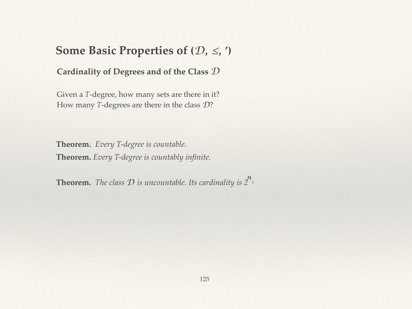
125

Theorem. Every T-degree is countable.Theorem. Every T-degree is countably infinite.

Theorem. The class D is uncountable. Its cardinality is 2 0

Some Basic Properties of (D, ≤, ’)

Cardinality of Degrees and of the Class D

א

Given a T-degree, how many sets are there in it? How many T-degrees are there in the class D?

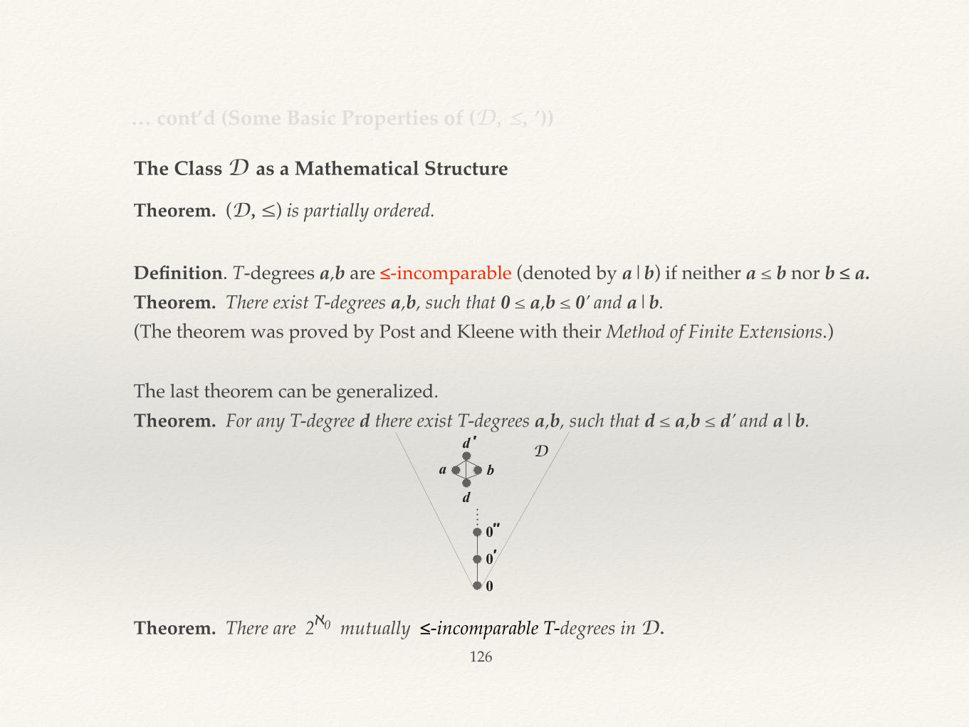
126

Theorem. (D, ≤) is partially ordered.

Definition. T-degrees a,b are ≤-incomparable (denoted by a|b) if neither a ≤ b nor b ≤ a. Theorem. There exist T-degrees a,b, such that 0 ≤ a,b ≤ 0’ and a|b.(The theorem was proved by Post and Kleene with their Method of Finite Extensions.)

The last theorem can be generalized.Theorem. For any T-degree d there exist T-degrees a,b, such that d ≤ a,b ≤ d’ and a|b.

Theorem. There are 2 0 mutually ≤-incomparable T-degrees in D.

… cont’d (Some Basic Properties of (D, ≤, ’))

The Class D as a Mathematical Structure

א

127

Since there are ≤-incomparable T-degrees, ≤ does not linearly order D. This gives rise to a series of questions about the existence of certain distinguished elements, such as minimal, least, greatest, maximal elements, upper bounds, lower bounds, least upper bounds, greatest lower bounds.

Theorem. There is a ≤-least T-degree in (D, ≤). This is the T-degree 0.

Theorem. Any two T-degrees have a ≤-least upper bound. Theorem. There is a pair of T-degrees that have no ≤-greatest lower bound.

Hence, (D, ≤) is not a lattice but an upper semi-lattice.


Distinguished T-Degrees

The Class D as a Mathematical Structure

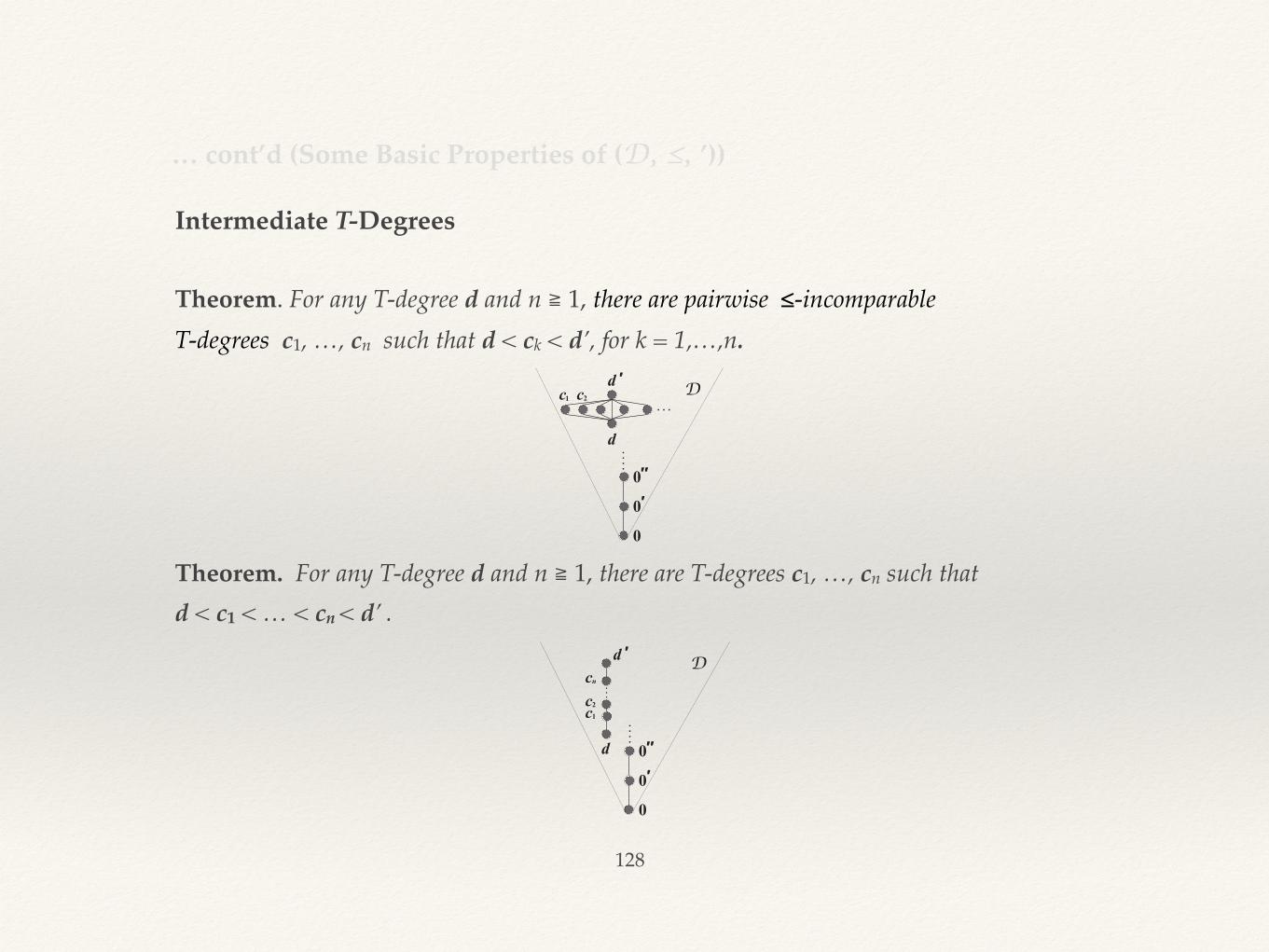
128

Theorem. For any T-degree d and n ≧ 1, there are pairwise ≤-incomparable T-degrees c1, …, cn such that d < ck < d’, for k = 1,…,n.

Theorem. For any T-degree d and n ≧ 1, there are T-degrees c1, …, cn such that d < c1 < … < cn < d’ .


Intermediate T-Degrees

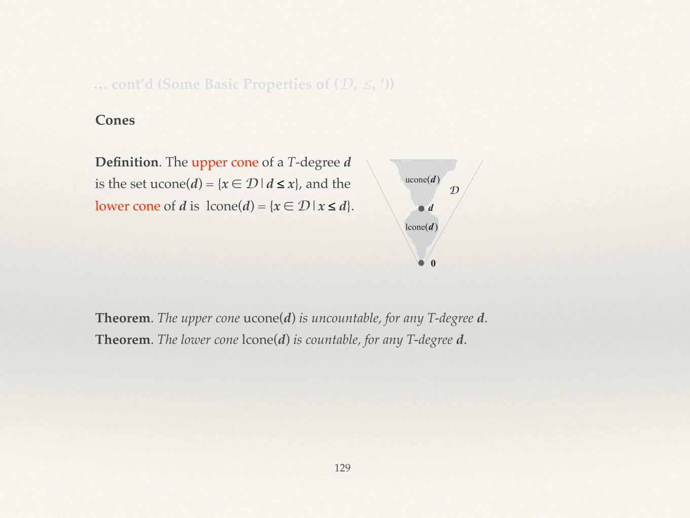
129

Definition. The upper cone of a T-degree d is the set ucone(d) = {x ∈ D|d ≤ x}, and the lower cone of d is lcone(d) = {x ∈ D|x ≤ d}.


Cones

Theorem. The upper cone ucone(d) is uncountable, for any T-degree d.Theorem. The lower cone lcone(d) is countable, for any T-degree d.

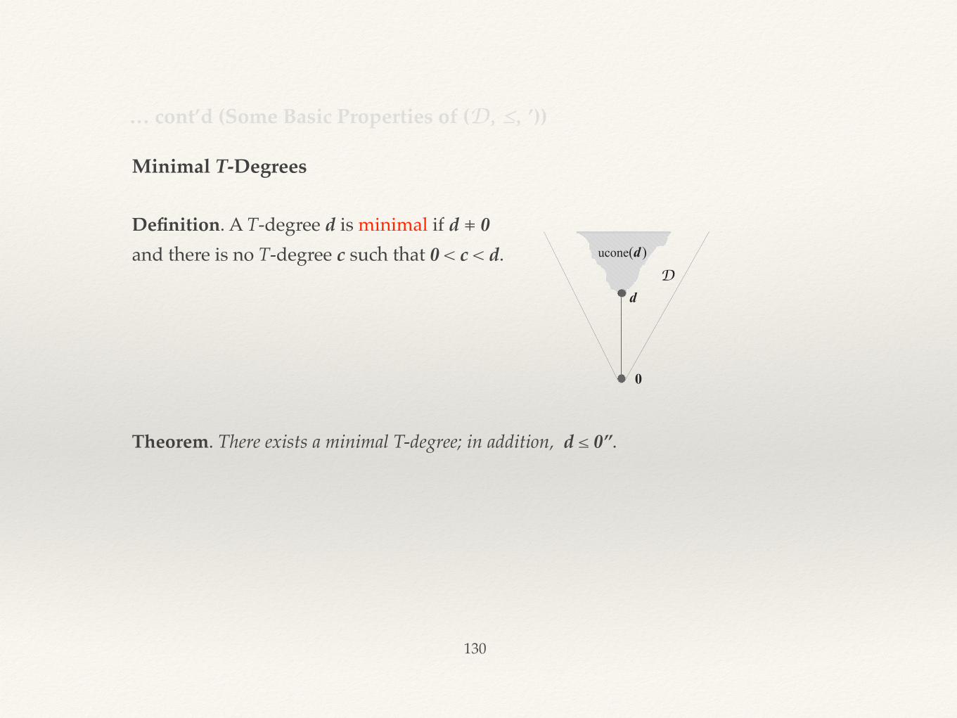
130

Definition. A T-degree d is minimal if d ⧧ 0 and there is no T-degree c such that 0 < c < d.


Minimal T-Degrees

Theorem. There exists a minimal T-degree; in addition, d ≤ 0’’.

Ch 14. C.E. Degrees and the Priority Method

❖ C.e. sets are important for they are undecidable and yet, in away, ``close’’ to the decidable sets.

❖ So are important T-degrees that stem from c.e. sets.

❖ Such T-degrees are called c.e. degrees.

131

132

Theorem. The set K is T-complete.

C.E. Turing Degrees

Completeness

Definition. Let ≤C be an arbitrary reducibility. A c.e. set S is said to be C-complete if A ≤C S for every c.e. set A.

C.E. Degrees

Definition. A T-degree is computably enumerable (c.e.) if it contains a c.e. set.

133

Post’s Problem

In 1944, Post asked whether there are any c.e. degrees strictly between 0 and 0’? Note that, informally, this is the question whether there exist undecidable problems that are less difficult than the Halting Problem.

Definition. (Post’s Problem) Is there a c.e. degree c such that 0 < c < 0’?

Post’s Program

However, Post did not succeed in attaining his program.

Post’s Problem was solved in 1956 by Friedberg and Muchnik who independently discovered and applied the Finite-Injury Priority Method.

To solve the problem, Post defined a list of goals that should be attained:

A. Define a property of a c.e. set.B. Prove that any set with this property is undecidable and T-

incomplete.C. Prove that there exist c.e. sets with this property.

134

In 1956, Friedberg and Muchnik simultaneously and independently upgraded the Post-Kleene’s Method of Finite Extensions into a subtler one, the Finite-injury Priority Method. By applying it, they obtained a positive answer to Post’s Problem.

The Priority Method in General

Let P be a property sensible of sets. Is there a c.e. set S with the property P?

The Priority Method tries to construct S step by step, in an infinite sequence of stages. At each stage i it constructs a finite set Si , an approximation of S. Each Si is obtained by adding new elements into Si-1 and/or banning certain elements from entering Si. So, we want to have Si-1 ⊆ Si for every i, and finally ∪i Si = S.

The basic guidelines are:

1. Rewrite P as R0 ⋀ R1 ⋀ R2 ⋀ … so that S will fulfil P iff S will fulfil every requirement Ri . An Ri can be fulfilled by carrying out finitely many instructions of the form ``add x into Si’’ or ``ban x from Si’’.

2. With different Rs associate different priorities, e.g. Ri-1 is of higher priority than Ri. 3. A fulfilled R can be injured, i.e., turned into unfulfilled, only by a higher-priority R.4. Allow any R to be injured only finitely many times.

The Priority Method and Priority Arguments

Ch 15. The Arithmetical Hierarchy

❖ There exists a different view of sets of natural numbers.

❖ This view allows us to define arithmetical classes of sets.

❖ It also gives rise to the Arithmetical hierarchy, the hierarchy of arithmetical classes.

❖ The hierarchy is closely connected with the Jump hierarchy.

135

136

Definition. A k-ary relation R on a set S is decidable (or semi-decidable, or undecidable) if the corresponding set R ⊆ Sk is decidable (or semi-decidable, or undecidable).

Decidability of Relations

Example. The relation R(e,x,s) ≣ ``Turing machine Te halts on x in at most s steps.’’ is decidable.

Theorem. A set A ⊆ ℕ is c.e. if and only if A = {x ∈ ℕ | ∃y R(x,y)} for some decidable relation R on ℕ.

137

Definition. A set A is an arithmetical set if A = {x ∈ ℕ|F(x)}, such that , for some n ≧ 0, the predicate F(x) = ∃y1∀y2 ∃y3 … Qyn R(x, y1, y2, y3 ,…, yn) or F(x) = ∀y1∃y2∀y3…Qyn R(x, y1, y2, y3 ,…, yn), and R is a decidable relation.

The Arithmetical Hierarchy

Theorem. For any n ≧ 0, the following hold: Σn ⊂ Σn+1

Σn ⊂ Πn+1

Πn ⊂ Πn+1

Πn ⊂ Σn+1

Δn ⊂ Σn

Δn ⊂ Πn

Definition. The arithmetical classes Σn, Πn, and Δn are defined as follows:Σn = class of all sets {x ∈ ℕ|F(x)}, where F(x) = ∃y1∀y2 ∃y3 … Qyn R(x, y1, y2, y3 ,…, yn) for some decidable relation R; Πn = class of all sets {x ∈ ℕ|F(x)}, where F(x) = ∀y1∃y2∀y3…Qyn R(x, y1, y2, y3 ,…, yn), for some decidable relation R;Δn = class of all sets {x ∈ ℕ|F(x)} that are in Σn ⋂ Πn.

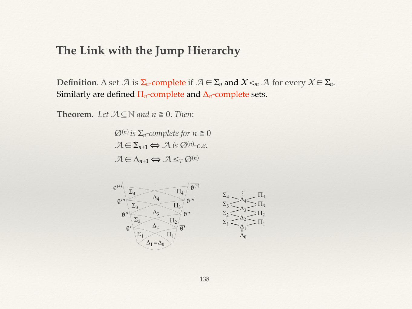
138

Definition. A set A is Σn-complete if A ∈ Σn and X <m A for every X ∈ Σn.Similarly are defined Πn-complete and Δn-complete sets.

The Link with the Jump Hierarchy

Theorem. Let A ⊆ ℕ and n ≧ 0. Then:

Ø(n) is Σn-complete for n ≧ 0A ∈ Σn+1 ⟺ A is Ø(n)-c.e. A ∈ Δn+1 ⟺ A ≤T Ø(n)

139

Empty slide.

Documents

University of Ljubljanalalg.fri.uni-lj.si/~borut/fct/lib/exe/fetch.php?media=fct-presentation.pdf · Ch 1. Introduction Deﬁnition. (algorithm intuitively) An algorithm for solving