Embed Size (px)
Citation preview

University College London
A computational study of
calcium carbonate
Thesis submitted for the degree of Doctor of Philosophy (PhD) by
Qi Wang
Supervised by
Prof. Nora H. de Leeuw
University College London
Department of Chemistry
September 2011

Declaration
2
Declaration
I, Qi Wang, confirm that this is my own work and the use of all materials from
other sources has been properly indicated in the thesis.
___________________
Qi Wang
September 2011
Abstract
3
Abstract
This thesis presents the results of computer simulation studies of impurity
incorporation in calcite and the aggregation of calcite particles, using a combination
of classical computational techniques based on interatomic potentials, namely
molecular mechanics and molecular dynamics simulations.
Firstly, the atomistic simulation techniques have been employed to investigate
the thermodynamics of mixing in calcite with seven divalent cationic impurities
(Mg2+
, Ni2+
, Co2+
, Zn2+
, Fe2+
, Mn2+
and Cd2+
), based on the calculation of all
inequivalent site occupancy configurations in 2 × 2 × 1 and 3 × 3 × 1 supercells of
the calcite structure. In addition to the enthalpy of mixing, the configurational
entropy and mixing free energy have also been calculated, providing an insight into
the mixing behaviour as a function of the temperature for a series of carbonate solid
solutions. The calculations have revealed that the solubility of the cationic impurities
in calcite is largely related to the cationic coordination distance with oxygen.
Secondly, the aggregation process has been investigated implementing classical
computational techniques, and especially the interaction of a calcite nanoparticle
with the major calcite surfaces, where the adhesion energy and optimised geometries
of a typical calcite nanoparticle on different surfaces in vacuum and aqueous
environment have been calculated. The results show the orientation of a nanoparticle
is a key factor that effects the interactions, besides the size and structure of the
nanoparticle. The most stable aggregated configuration occurs when the lattices of
the nanoparticle and the surface are perfectly aligned.

Abstract
4
Finally, a number of symmetric calcite tilt grain boundaries have been
constructed to act as models of two calcite nanoparticles, after collision has occurred
but before growth has a chance to commence. Molecular dynamics simulations were
then employed to study the stability of these tilt grain boundaries and the growth of a
series of calcium carbonate units at the contact points in the pure and hydrated calcite
tilt grain boundaries. The calculation have proved that the initial incorporation of a
CaCO3 unit is preferential at the obtuse step in a grain boundary, and the growth
velocity of the acute step is 1.3 to 2.1 times higher than that of the obtuse step, once
the initial growth unit has been deposited on the steps. This study has evaluated the
conditions required for the growth of new calcium carbonate materials in the calcite
tilt grain boundaries.

List of Publications
5
List of Publications
The work described in this thesis has been published in the following papers:
Qi Wang, Ricardo Grau-Crespo and Nora H. de Leeuw (2011) Mixing
thermodynamics of the calcite-structured (Mn,Ca)CO3 solid solution: A computer
simulation study. Journal of Physical Chemistry C, accepted.
Qi Wang and Nora H. de Leeuw (2009) A computer simulation study of the
thermodynamics of mixing in the (Mn,Ca)CO3 solid solution. Geochimica et
Cosmochimica Acta, Vol. 73: A1412.
Qi Wang and Nora H. de Leeuw (2008) A computer modelling study of
CdCO3-CaCO3 solid solutions. Mineralogical Magazine, Vol. 72: 525-529.

Acknowledgement
6
Acknowledgement
First of all, I would like to thank my supervisor, Prof. Nora H. de Leeuw, for her
distinguished guidance and generous support during the past four years. This thesis
really wouldn‟t have been possible without her supervision.
Particular thanks should go to Dr. Zhimei Du and Dr. Ricardo Grau-Crespo, for
their invaluable guidance and helpful discussion throughout this project. I would like
to give my acknowledgement to the whole group, where I received lots of help and
encouragements. A special thank you to Prof. Steve Parker, who gave me lots of kind
help and guidance during my visit in Bath University.
I am grateful to the China Scholarship Council (CSC) for financial support and
University College London for an Overseas Research Studentship. I also thank the
EU-funded “Mineral Nucleation and Growth Kinetics (MIN-GRO) Marie-Curie
Research and Training Network” for funding. I also acknowledge the use of the UCL
Legion High Performance Computing Facility and associated support services in the
completion of this project.
Finally, I sincerely thank my grandparents, parents and fiancée Dr. Qiyao Feng
for showing concerns, giving loves and support to me during my four years PhD
study in UCL. I would like to dedicate this thesis to them. Thank you very much.

Table of Contents
7
Table of Contents
DECLARATION ....................................................................................................................... 2
ABSTRACT ................................................................................................................................ 3
LIST OF PUBLICATIONS .................................................................................................... 5
ACKNOWLEDGEMENT ...................................................................................................... 6
TABLE OF CONTENTS ........................................................................................................ 7
LIST OF FIGURES ............................................................................................................... 20
LIST OF TABLES ................................................................................................................. 20
LIST OF ABBREVIATIONS ............................................................................................. 20
Chapter 1 Introduction ........................................................................................ 21
1.1 Calcium carbonate ....................................................................................................... 22
1.2 Incorporation of impurities in calcium carbonate ................................................. 24
1.2.1 Heavy metals in nature ........................................................................ 26
1.2.2 Carbonate solid solutions ..................................................................... 27
1.2.3 Experimental studies of carbonate solid solutions ................................ 29
1.2.4 Theoretical studies of carbonate solid solutions.................................... 31
1.3 The growth and dissolution of calcium carbonate ................................................ 34
1.3.1 Nucleation and growth of calcium carbonate........................................ 34
1.3.2 Dissolution of calcite ........................................................................... 37
1.4 Aggregation of calcite nanoparticles ....................................................................... 38
1.5 Aims and overview of the thesis ............................................................................... 41
Chapter 2 Computational Methodology ............................................................. 43
2.1 Molecular mechanics .................................................................................................. 44
2.1.1 Potential energy surface ....................................................................... 44
2.1.2 Energy minimisation algorithm ............................................................ 45

Table of Contents
8
2.1.3 Static lattice optimisation ..................................................................... 48
2.1.4 Surface simulations.............................................................................. 50
2.1.5 Construction of calcite nanoparticles ................................................... 55
2.2 Molecular dynamics .................................................................................................... 56
2.2.1 Finite difference methods..................................................................... 57
2.2.2 Ensembles ........................................................................................... 60
2.2.3 Periodic boundary conditions ............................................................... 61
2.2.4 Running MD simulations ..................................................................... 62
2.2.5 Analysis ............................................................................................... 65
Chapter 3 Potential models.................................................................................. 67
3.1 The Born model of solids ........................................................................................... 68
3.2 The Ewald method ....................................................................................................... 69
3.3 Electronic polarisability ............................................................................................. 70
3.4 Short range potential functions ................................................................................. 72
3.4.1 Buckingham potential function ............................................................ 72
3.4.2 Morse potential function ...................................................................... 73
3.4.3 Lennard-Jones potential function ......................................................... 74
3.4.4 Many body potential function .............................................................. 74
3.5 Potentials of carbonates and water ........................................................................... 76
3.6 Derivation of potentials for Ni, Co, Zn and Mn carbonates ............................... 78
Chapter 4 Mixing thermodynamics of calcite with divalent cation impurities .. 82
4.1 Introduction ................................................................................................................... 83
4.2 Configurational statistics............................................................................................ 85
4.3 Structure and configurational entropy ..................................................................... 89
4.4 MnCO3-CaCO3 solid solutions ................................................................................. 94
4.5 CdCO3-CaCO3 solid solutions ................................................................................ 104
4.6 FeCO3-CaCO3 solid solutions ................................................................................. 109
4.7 Uptake of Zn2+
and Co2+
to calcite ......................................................................... 113
4.8 Uptake of Mg2+
and Ni2+
to calcite ......................................................................... 115

Table of Contents
9
4.9 Chapter summary ....................................................................................................... 119
Chapter 5 Investigation of the interaction between calcite nanoparticle and
calcite surfaces ....................................................................................................121
5.1 Introduction ................................................................................................................. 122
5.2 Calcite surfaces .......................................................................................................... 122
5.3 Calcite nanoparticle ................................................................................................... 129
5.4 Adhesion energy of a nanoparticle on the surface .............................................. 130
5.5 Interaction between a nanoparticle104 and calcite surfaces ............................... 132
5.5.1 Nanoparticle104 and pure {10 4} surface ............................................134
5.5.2 Nanoparticle104 and hydrated {10 4} surface ......................................136
5.5.3 The effect of the size of a nanoparticle104 ............................................141
5.5.4 Nanoparticle104 and pure {0001} surface.............................................142
5.5.5 Nanoparticle104 and hydrated {0001} surface ......................................146
5.5.6 Nanoparticle104 and stepped surfaces ..................................................149
5.6 Interaction between a nanoparticle001 and calcite surfaces ............................... 153
5.6.1 Nanoparticle001 and pure {10 4} surface ............................................155
5.6.2 Nanoparticle001 and hydrated {10 4} surface ......................................156
5.6.3 Nanoparticle001 and pure {0001} surface.............................................159
5.6.4 Nanoparticle001 and hydrated {0001} surface ......................................163
5.7 Chapter summary ....................................................................................................... 164
Chapter 6 The growth of calcium carbonate at tilt grain boundaries and stepped
surfaces ................................................................................................................166
6.1 Introduction ................................................................................................................. 167
6.2 Methods ....................................................................................................................... 169
6.3 Tilt grain boundaries of calcite ............................................................................... 172
6.4 Single calcium carbonate unit in aqueous environment .................................... 179
6.5 The growth of calcium carbonate in pure grain boundaries ............................. 181
6.6 The growth of calcium carbonate in hydrated grain boundaries...................... 186
6.7 Chapter summary ....................................................................................................... 191

Table of Contents
10
Chapter 7 Conclusions and Future works..........................................................193
7.1 Conclusions ................................................................................................................. 194
7.1.1 The incorporation of cationic impurities in calcite ...............................194
7.1.2 The adhesion of calcite nanoparticle on calcite surface .......................195
7.1.3 The growth of calcium carbonate units in tilt grain boundary ..............195
7.2 Future works ............................................................................................................... 198
BIBLIOGRAPHIC .............................................................................................200

List of Figures
11
List of Figures
Figure 1.1: Illustration of orthorhombic double cells of aragonite, (a) side view, and
(b) top view, (Ca = green, O = red, C = grey). ........................................................ 23
Figure 1.2: Hexagonal representation of a calcite unit cell, (a) side view, and (b) top
view (Ca = green, O = red, C = grey). .................................................................... 24
Figure 1.3: Illustration of {10 4} and {0001} planes of calcite. The {0001} plane
has two terminations, i.e. a Ca2+
termination and a CO32-
termination. .................... 25
Figure 1.4: Photographs of crystals of (a) manganocalcite (MnxCa1-xCO3) from
Yunnan, China and (b) rhodochrosite (MnCO3) from Chihuahua, Mexico. ............. 28
Figure 1.5: Growth morphology of calcite as a function of the Ca2+
/CO32-
ratio. (a)
At low Ca2+
/CO32-
ratio, the obtuse steps do not advance. Both step orientations have
a high kink density, as evidenced by their roughness. (b) At intermediate ratios, both
obtuse and acute step orientations are straight and advance. (c)At high ratios, the
obtuse step orientation continues to grow, whereas the acute step has become pinned
and etch-pits are observed, (Stack and Grantham, 2010)......................................... 36
Figure 1.6: SEM images of micro-sized aggregated CaCO3 particles, (Collier et al.,
2000). .................................................................................................................... 39
Figure 2.1: Local minimum and global minimum on a potential energy surface..... 45
Figure 2.2: Side view of two types of surfaces as classified by Tasker. (a) Type I
surface consisting of charge neutral layers, and (b) Type II surface consisting of
positive and negative charged planes but with a charge neutral and non-dipolar repeat
unit. The dashed line representatives the two dimensional periodicity. .................... 51
Figure 2.3: Stacking sequences showing (a) a Type III surface, consisting of
alternating positive and negative ions giving rise to a dipolar repeat unit, and (b) a
reconstructed Type III surface, where half the surface ions have been moved to the
bottom of the surface in order to remove the net dipole. The dashed line
representatives the two dimensional periodicity. ..................................................... 52
Figure 2.4: The two region approach used in METADISE, (a) a crystal; (b) the
complete crystal containing two blocks and (c) half a crystal, exposing a surface. .. 53
Figure 2.5: (a) Calcite crystal growing from the aqueous solution (Didymus et al.,
1993) and (b) equilibrium morphology of calcite particle constructed by the Wulff
construction method. .............................................................................................. 56

List of Figures
12
Figure 2.6: A two-dimensional periodic system. Molecules can enter and leave each
box across each of the four edges. In a three-dimensional system, molecules would
be free to across any of the six cube faces (Allen & Tildesley, 1999). ..................... 62
Figure 3.1: Plots showing the variation in the long-range, short-range and total
potential energies as a function of rij for a Ca2+
-O2-
ion pair. ................................... 68
Figure 3.2: Schematic representation of the core-shell model: (a) no displacement,
unpolarised. (b) displacement, polarised. The blue sphere, representing the core, has
the charge Xe. The open grey sphere, representing the shell, has the charge of Ye. The
core and shell are connected by a spring of force constant K, (Murphy, 2009). ....... 71
Figure 3.3: The three-body interaction in a carbonate group. ................................. 75
Figure 3.4: The four-body interaction of four atoms lying in two planes with a
torsional angle θ. .................................................................................................... 75
Figure 4.1: The structures of the most stable configurations for x = n/6 (n = 1, 2, 3).
The lowest-energy structures for n = 4 and 5 can be obtained from the ones with n =
2 and 1, respectively, if Ca2+
and impurity Me2+
positions are swapped. The n = 3
case (x = 0.5) corresponds to the ordered dolomite-type structure. (Ca = green, C =
grey, O = red, Me = blue). ...................................................................................... 90
Figure 4.2: The lowest (black line) and highest (blue line) lattice energies of mixed
systems for Me2+
composition x = 0.25, compared to the average lattice energy in the
configurational space (red line). ............................................................................. 91
Figure 4.3: Configurational spectrum of lattice energies corresponding to the
composition of Cd0.25Ca0.75CO3 at 300 K, as calculated in a 2 × 2 × 1 supercell. .... 91
Figure 4.4: Variation of the configurational entropy corresponding to the
composition of Me0.33Ca0.67CO3 at 300 K, as calculated in a 2 × 2 × 1 supercell. .... 93
Figure 4.5: Variation of the maximum configurational entropy (in the full disorder
limit) with the supercell size. ................................................................................. 93
Figure 4.6: Calculated and experimental mixing enthalpies for the Ca-rich
MnxCa1-xCO3 solid solution. The empty squares in red colour correspond to
calculations in the full disorder limit with the 3 × 3 × 1 supercell. .......................... 97
Figure 4.7: Calculated and experimental mixing enthalpies for the Mn-rich
MnxCa1-xCO3 solid solution. The empty squares in red colour correspond to
calculations in the full disorder limit with the 3 × 3 × 1 supercell. .......................... 98
Figure 4.8: The structure of kutnahorite, showing Mn2+
and Ca2+
occupy alternating
interlayers. (Ca = green, Mn = purple, C = grey, O = red). .....................................100
Figure 4.9: The variation of enthalpy of mixing with different number of
Mn0.5Ca0.5CO3 configurations at 3000 K and infinitely high temperature. ..............101

List of Figures
13
Figure 4.10: The different in free energy ΔG between the disordered Mn0.5Ca0.5CO3
and kutnahorite as a function of temperature. The negative G indicates the
disordered Mn0.5Ca0.5CO3 is more stable than ordered kutnahorite at this temperature.
. ............................................................................................................................102
Figure 4.11: Calculated free energy of mixing with full range of Mn2+
compositions
at 900 K. ...............................................................................................................103
Figure 4.12: Variation of the lattice parameters of MnxCa1-xCO3 as a function of
composition, in comparison with experiment (Katsikopoulos et al., 2009). ...........104
Figure 4.13: The variation of enthalpy of mixing with different number of
inequivalent Cd0.5Ca0.5CO3 configurations at 300 K and1000 K. ...........................106
Figure 4.14: Calculated mixing enthalpy and mixing free energy of the CdxCa1-xCO3
system as a function of Cd2+
composition, as calculated for a 2 × 2 × 1 supercell. .107
Figure: 4.15: Comparison between theoretical and experimental excess free energies
GE findings for CdxCa1-xCO3 at 300 K. ..................................................................108
Figure 4.16: Calculated enthalpy of mixing in the FexCa1-xCO3 system. The solid
lines show the enthalpy isotherms between 300 K and 1500 K with a step of 300 K.
The dashed lines show the enthalpy at an infinitely high temperature. ...................110
Figure 4.17: Calculated free energy of mixing of the FexCa1-xCO3 system as a
function of Fe2+
compositions. ..............................................................................111
Figure 4.18: Comparison between theoretical excess Gibbs free energies GE for the
FexCa1-xCO3 solid solutions at 823 K. ....................................................................112
Figure 4.19: Calculated free energy of mixing with full range of Co2+
or Zn2+
compositions; (a) CoxCa1-xCO3, (b) ZnxCa1-xCO3 ...................................................114
Figure 4.20: Calculated free energy of mixing of the binary (Mg,Ca)CO3 system as a
function of Mg2+
composition, (a) calcite-dolomite, (b) dolomite-magnetite. .........118
Figure 4.21: Calculated free energy of mixing of the binary systems as a function of
Ni2+
composition. (a) CaCO3-Ca0.5Ni0.5CO3, (b) Ca0.5Ni0.5CO3-NiCO3 ..................119
Figure 5.1: Top view and side view of pure planar surfaces, (a) {10 4} surface, (b)
CO32-
terminated {0001} surface and (c) Ca2+
terminated {0001} surface. (Ca =
green, C = grey, O = red). ......................................................................................124
Figure 5.2: Side view of pure stepped surfaces, (a) acute {3 1 8} surface and (b)
obtuse {3 16} surface. (Ca = green, C = grey, O = red). ...............................125
Figure 5.3: Top view and side view of hydrated planar surfaces with monolayer of
water, (a) {10 4} surface, (b) CO32-
terminated {0001} surface and (c) Ca2+
terminated {0001} surface. (Ca = green, C = grey, O = red, H = white, Owater = blue).
.............................................................................................................................127

List of Figures
14
Figure 5.4: Side view of hydrated stepped surfaces with monolayer of water, (a)
acute {3 1 8} surface and (b) obtuse {3 16} surface (Ca = green, C = grey,
O = red, H = white, Owater = blue) ..........................................................................128
Figure 5.5: Morphology of CaCO3 nanoparticle, showing (a) {10 4} surface (b)
{0001}-Ca2+
surface and (c) {0001}-CO32-
surface. ..............................................130
Figure 5.6: Examples of a calcite nanoparticle104 on the top plane of planar {10 4}
surface. (Ca = green, C = grey, O = red). ...............................................................131
Figure 5.7: The variation of unrelaxed adhesion energies with distance between pure
{10 4} surface and a calcite nanoparticle104 in vacuum. Results for some orientations
have been omitted for clarity. ................................................................................134
Figure 5.8: 3-D and 2-D adhesion energy contour of the nanoparticle104 on the pure
{10 4} surface with a rotation of (a) and (b) θ = 0o, (c) and (d) θ = 180
o. (Ca = green,
C = grey, O = red). ................................................................................................135
Figure 5.9: Adhesion energy as a function of the distance between the monolayer
hydrated {10 4} surface and a nanoparticle104. Results for some orientations have
been omitted for clarity. ........................................................................................136
Figure 5.10: Adhesion energy as a function of the orientation of a nanoparticle104 on
pure (black triangle) and hydrated (red circle) {10 4} surface. .............................137
Figure 5.11: 3-D and 2-D adhesion energy contours of the nanoparticle104 on the
hydrated {10 4} surface with a rotation of θ = 0o. (Ca = green, C = grey, H = white,
O = red, Owater = blue). ..........................................................................................138
Figure 5.12: Side view of the unrelaxed interfacial system of the monolayer hydrated
{10 4} surface/calcite nanoparticle104 at a rotation of 0o. (Ca = green, C = grey, O =
red, Owater = blue, H = white). ................................................................................139
Figure 5.13: Adhesion energy as a function of the distance between the hydrated
{10 4} surface with multilayer water and the nanoparticle104 at a rotation of 0o. ...140
Figure 5.14: The twist pathway of a nanoparticle104 through the multilayer water,
where Pi (i = 1, 2, 3 and 4) is the position of local energy minimum. .....................140
Figure 5.15: Unrelaxed adhesion energies as a function of the orientations of the
nanoparticle104 for the pure (triangle) and monolayer hydrated (circle) {10 4}
interfacial systems, (d = 1.0 nm: black line, d = 1.3 nm: red line). .........................141
Figure 5.16: Adhesion energy as a function of the distance between the pure {0001}
surface and a nanoparticle104. Results for some orientations have been omitted for
clarity. ...................................................................................................................143
Figure 5.17: Adhesion energy as a function of the orientation of a nanoparticle104 on
pure {0001} surfaces.............................................................................................144

List of Figures
15
Figure 5.18: 2-D adhesion energy contour of the nanoparticle104 on the pure {0001}
surface with a rotation of θ = 0o, (a) CO3
2- termination and (b) Ca
2+ termination. ..145
Figure 5.19: Side view of the top plane of (a) {0001}-CO32-
surface, (b) {0001}-Ca2+
surface and (c) {10 4} surface, (Ca = green, C = grey, O = red)............................146
Figure 5.20: Adhesion energy as a function of the distance between the monolayer
hydrated {0001} surface and a nanoparticle104. Results for some orientations have
been omitted for clarity. ........................................................................................147
Figure 5.21: Adhesion energy as a function of the distance between the multilayer
hydrated {0001} surface and the nanoparticle104 at a rotation of 0o. .......................147
Figure 5.22: The twist pathway of a nanoparticle104 through the multilayer water,
where Pi is the position of local energy minimum, (a) {0001}-CO32-
surface, from P1
to P4; (b) {0001}-Ca2+
surface, from P1 to P3. ........................................................148
Figure 5.23: Side view of the unrelaxed interfacial systems of a nanoparticle104 on
the pure stepped surface, (a) acute stepped {3 1 8} surface and (b) obtuse stepped
{3 16} surface, where the nanoparticle is at a rotation of 0o with respect to the
terraces of the stepped surfaces (Ca = green, O = red, C = grey). ...........................150
Figure 5.24: The variation of adhesion energy as the nanoparticle104 moving along
the step wall of pure {3 1 8} surface (black line) and planar {10 4} surfaces (red
line). .....................................................................................................................151
Figure 5.25: Adhesion energy as a function of the height between a nanoparticle104
and the hydrated planar and stepped surfaces. .......................................................152
Figure 5.26: Adhesion energy as a function of the distance between the pure {10 4}
surface and a nanoparticle001. Results for some orientations have been omitted for
clarity due to the periodic reiteration. ....................................................................156
Figure 5.27: Side view of the most stable interfacial configurations of the pure
{10 1 4} surface with a calcite nanoparticle001. (a) nanoparticle001-Ca and (b)
nanoparticle001-CO3, (Ca = green; C = grey; O = red). .............................................157
Figure 5.28: Adhesion energy as a function of the distance between the hydrated
{10 4} surface and nanoparticle001. Results for other orientations have been omitted
for clarity. .............................................................................................................158
Figure 5.29: Side view of the most stable interfacial configuration of the hydrated
{10 4} surface with a nanoparticle001-CO3 (a 0o rotation), where the blue dashes lines
show the hydrogen bonds, (Ca = green, C = grey, O = red, Owater = blue, H = white).
.............................................................................................................................159
Figure 5.30: Adhesion energy as a function of the distance between a nanoparticle001
and pure {0001} surface. Results for other orientations have been omitted for clarity.
.............................................................................................................................160

List of Figures
16
Figure 5.31: Side view of the most stable interfacial configurations of the pure
{0001} surface with a nanoparticle001-Ca. (a) Ca2+
termination and (b) CO32-
termination, (Ca = green; C = grey; O = red). ........................................................161
Figure 5.32: Adhesion energy as a function of the orientation of the nanoparticle001
on pure {0001} surfaces. A nanoparticle001-Ca on the {0001}-CO32-
surface (red line
and circle) and {0001}-Ca2+
surface (black line and triangle); a nanoparticle001-CO3 on
the {0001}-CO32-
surface (green line and circle) and {0001}-Ca2+
surface (blue line
and triangle). .........................................................................................................162
Figure 5.33: Adhesion energy as a function of the orientation of the nanoparticle001
on hydrated {0001} surface: {0001}-CO32-
surface (circle) and {0001}-Ca2+
surface
(triangle). ..............................................................................................................163
Figure 6.1: Side views of the unrelaxed calcite tilt grain boundaries: (a) A-grain
boundary and (b) O-grain boundary. The surface area of each {10 4} terrace
between the steps is 620.9 Å2. (Ca = green, C = gray, O = red). .............................170
Figure 6.2: Side view of relaxed calcite grain boundaries: (a) A-grain boundary and
(b) O-grain boundary. The surface area of the {10 4} terrace is 1241.8 Å2. (Ca =
green, C = gray, O = red). ......................................................................................173
Figure 6.3: Snapshot of hydrated grain boundaries after 250 ps MD simulations,
where four distinct Ca2+
sites are labelled in the interfacial regions. The Ca2+
in the
acute step of the joints are labelled Caa-j; the Ca2+
in the obtuse step of the joints are
labelled Cao-j; the Ca2+
at the step of original stepped surface are labelled Cac, and
Cat stands for the Ca2+
in the middle of the terraces. (a) A-grain boundary and (b)
O-grain boundary. (Ca = green, O = red, C = grey, Owater = red, H = white). ..........176
Figure 6.4: Radial distribution functions (RDF) for the local environment in the
water at structurally different Ca2+
surface sites. (a) A-grain boundary and (b)
O-grain boundary. .................................................................................................178
Figure 6.5: Representative snapshot from the MD simulations taken at 10 ps. (Ca =
green; C = grey; O = red; H = white). ....................................................................180
Figure 6.6: Radial distribution functions (RDF) of the Ca2+
-Ocarbonate and Ca2+
-Owater.
.............................................................................................................................181
Figure 6.7: Initial structures of the O-grain boundary with single CaCO3 unit in
vacuum. The CaCO3 unit was added at four different positions (P-I, I = 1, 2, 3 and 4)
in the channel void, respectively. ...........................................................................183
Figure 6.8: Schematic diagram of the incorporation of the first and second CaCO3
units along the step in the grain boundary. (Ca = green, C = black, O = red). .........183
Figure 6.9: The growth energies of addition of successive CaCO3 units at the steps of
the joints (Position-1 and Position-2) in the A-grain boundary and O-grain boundary
in vacuum. ............................................................................................................185

List of Figures
17
Figure 6.10: Bar charts of the average growth energies per CaCO3 unit released upon
the growth of a full CaCO3 row in the A-grain boundary and O-grain boundary. ...186
Figure 6.11: The energies of addition of successive CaCO3 units at the steps of the
joints (Position-1 and Position-2) in the A-grain boundary and O-grain boundary
under aqueous conditions. .....................................................................................189
Figure 6.12: Bar charts of the average growth energies per CaCO3 unit released upon
the growth of a full CaCO3 row at the hydrated A-grain boundary and O-grain
boundary systems. .................................................................................................190

List of Tables
18
List of Tables
Table 3.1 Potential parameters used in this thesis (short-range cutoff 20 Å). .......... 77
Table 3.2 Interionic Buckingham potentials obtained from fits to NiCO3, CoCO3,
MnCO3 and ZnCO3 structures and enthalpies of reaction 3.14. ............................... 80
Table 3.3 Calculated and experimental properties of NiCO3, CoCO3, ZnCO3, MnCO3
and CaCO3. ............................................................................................................ 81
Table 4.1 Total number of configurations (W) and number of symmetrically
inequivalent configurations (M) for each composition MexCa1-xCO3 in 2 × 2 × 1 and
3 × 3 × 1 supercells (A and B stand for either Ca or impurity). ............................... 88
Table 4.2 Some data on rhombohedral carbonates. ................................................120
Table 5.1 Surface energies of pure calcite surfaces (Jm-2
) .....................................123
Table 5.2 Surface energies of hydrated calcite surfaces (Jm-2
) ...............................126
Table 5.3 Unrelaxed adhesion energies of a calcite nanoparticle104 on the calcite
planar surfaces in vacuum and aqueous solution. ...................................................133
Table 5.4 Relaxed adhesion energies of a calcite nanoparticle104 on the calcite planar
surfaces in vacuum and aqueous solution. .............................................................133
Table 5.5: The lowest unrelaxed adhesion energy of a nanoparticle104 to the planar
{10 4} and stepped {3 1 8}, {3 16} surfaces. ..........................................150
Table 5.6 Unrelaxed adhesion energies of a calcite nanoparticle001-Ca on the calcite
planar surfaces in vacuum and aqueous solution. ...................................................154
Table 5.7 Unrelaxed adhesion energies of a calcite nanoparticle001-CO3 on the calcite
planar surfaces in vacuum and aqueous solution. ...................................................155
Table 6.1 Boundary and cleavage energies of the non-hydrated grain boundaries. .174
Table 6.2 Boundary and hydration energies of the hydrated grain boundaries........175
Table 6.3 Local environment of Ca2+
ions at structurally different positions in the
hydrated grain boundaries. The distance listed here are from RDF results. ............177
Table 6.4 Average configurational energies for the CaCO3 unit in vacuum and water,
and liquid water following simulations at 300 K for 0.2 ns. ...................................180
Table 6.5 Growth energies of incorporation of CaCO3 units at various growth sites

List of Tables
19
on the two non-hydrated grain boundaries (kJmol-1
). .............................................184
Table 6.6 Growth energies of incorporation of CaCO3 units at various growth sites in
the hydrated A-grain boundary and O-grain boundary, as calculated by equation 6.6
(kJmol-1
). ..............................................................................................................187
Table 6.7 Growth energies of incorporation of CaCO3 units at various growth sites in
the hydrated A-grain boundary and O-grain boundary, as calculated by equation 6.7
(kJmol-1
). ..............................................................................................................188

List of Abbreviations
20
List of Abbreviations
AFM Atomic Force Microscopy
BCCF The British Calcium Carbonates Federation
BFGS Broyden Fletcher Goldfarb Shanno
DFT Density Functional Theory
GULP General Utility Lattice Program
IMANA The Industrial Minerals Association North America
LEED Low Energy Electron Diffraction
MC Monte Carlo
MD Molecular Dynamics
MM Molecular Mechanics
NPT Constant Number, Pressure and Temperature
NST Constant Number, Pressure and Temperature
NVE Constant Number, Volume and Energy
NVT Constant Number, Volume and Temperature
PBC Periodic Boundary Condition
PES Potential Energy Surface
RDF Radial Distribution Function
SEM Scanning Electron Microscopy
SOD Site Occupancy Disorder
TEM Transmission Electron Microscopy
XPS X-ray Photoelectron Spectroscopy
XRD X-Ray Diffraction
WAXS Wide Angle X-ray Scattering

21
1 Introduction
Calcium carbonate is one of the most abundant minerals in our environment. It
has been studied for more than a century because of its important role in geochemical,
biological and industrial processes. This chapter gives a brief description of two
important topics: the incorporation of cationic impurities in calcium carbonate and
the growth and dissolution of calcium carbonate, where both experimental studies
and computer modelling investigations are included. It also introduces the objectives
of this thesis and provides an overview of the subsequent chapters.

Chapter 1: Introduction
22
1.1 Calcium carbonate
Calcium carbonate (CaCO3) is one of the most abundant materials found in
sedimentary rock in all parts of the Earth surface. CaCO3 makes up 4% of the earth's
crust and forms the rock types like limestone and chalk. Limestone makes up about
10% of all sedimentary rocks and is composed largely of the minerals calcite and
aragonite (different crystal forms of CaCO3). Chalk is a white sedimentary rock, a
form of limestone composed of the mineral calcite (Frye, 1981; Deer et al., 1992).
CaCO3 is also an important component in biological systems, such as shells of
marine organisms, pearls and egg shells (Beruto and Giordani, 1993).
CaCO3 has been the subject of extensive and varied research because of its
fundamental applications in industrial, pharmaceutical and environmental fields.
CaCO3 is a common raw substance in the construction industry, both as a building
material (e.g. marble) and as an ingredient of cement. Because of its antacid
properties, CaCO3 is also used to neutralize acidic conditions in both water and soil
in industrial fields (BCCF, 2007; IMANA, 2010). CaCO3 is widely used as fillers in
paper, rubber, plastics and paints to improve relevant mechanical properties of
industrial materials (Zuiderduin et al., 2003; Rocha et al., 2005). It is also used as a
carbon isotope counter in marine carbonates, with a view to assessing the
relationship between carbon-induced emission and climate change (Romanek et al.,
1992). As a dietary supplement, CaCO3 is an inexpensive calcium source or gastric
antacid in the pharmaceutical industry (Lieberman et al., 1990; Gabriely et al., 2008).
Furthermore, CaCO3 has been shown to chemically interact with various solvated
heavy ions, such as Fe2+
, Cd2+
and Mn2+
(Stipp and Hochella, 1991; Stipp, 1998;
Park et al., 1996), and some organic molecules when exposed to aqueous solutions
(Lebron and Suarez, 1998; Hoch et al., 2000). Hence CaCO3 can be applied in water

Chapter 1: Introduction
23
treatment because of its strong surface interaction with heavy metals in the
environment.
CaCO3 exists in nature as several polymorphs: amorphous calcium carbonate,
ikaite (CaCO3·6H2O), vaterite, aragonite and calcite. Both amorphous CaCO3 and
ikaite are metastable in the environment and change easily to the more stable
polymorph calcite (Deer et al., 1992; Chang et al., 1996). Vaterite (µ-CaCO3) is also
a metastable phase of CaCO3 at ambient conditions at the surface of the Earth. Once
vaterite is exposed to water, it converts to aragonite or calcite (Palache et al., 1951).
(a) (b)
Figure 1.1: Illustration of orthorhombic double cells of aragonite, (a) side view, and
(b) top view, (Ca = green, O = red, C = grey).
Aragonite is one of the two common, naturally occurring polymorph of CaCO3.
It is formed by biological and physical processes, including precipitation from
marine and freshwater environments. In particular, aragonite is the major constituent
of coral reefs, shells, pears and other biominerals, where it grow preferentially at
ambient conditions due to the effect of organic templates (Morse and Mackenzie,
Z
X
X
Y

Chapter 1: Introduction
24
1990). Aragonite is thermodynamically unstable at standard temperature and pressure,
and tends to alter to calcite over geologic time (Chang et al., 1996). Aragonite has an
orthorhombic crystal structure with space group Pmcn. The experimental structure
found by Dickens and Bowen (1971) is a = 4.960 Å, b = 7.964 Å, and c = 5.738 Å
and α = β = γ = 90º, containing four CaCO3 (Figure 1.1).
(a) (b)
Figure 1.2: Hexagonal representation of a calcite unit cell, (a) side view, and (b) top
view (Ca = green, O = red, C = grey).
Calcite is the most common and stable form of CaCO3 in the environment. It is
stable at atmospheric pressure and temperature and only decomposes at 973 K,
becoming calcium oxide (Kuriyavar et al., 2000). The rhombohedral crystal structure
of calcite was firstly determined using X-ray diffraction (XRD) by Bragg in 1914.
The rhombohedral crystal structure can be defined using hexagonal axes and calcite
surface are usually referred to using hexagonal indices, where four Miller indices are
used instead of three and this convention is followed in this thesis. The hexagonal
unit cell of calcite has a = b = 4.990 Å, c = 17.061 Å, and α = β = 90o, γ = 120
o (Deer
et al., 1992), shown in Figure 1.2. The CO32-
groups in calcite are arranged
Z
X
Y
X

Chapter 1: Introduction
25
differently to the corresponding groups in aragonite. Unlike in aragonite, the CO32-
groups do not lie in two layers that point in opposite directions. Instead they lie in a
single plane pointing in the same direction, showing alternating layering of planar
CO32-
groups and Ca2+
ions. Each oxygen atom in CO32-
group is surrounded by two
Ca2+
ions in the calcite and three in aragonite (Bragg, 1924).
The Ca2+
and CO32-
ions in calcite are held together through ionic bonding and it
is easy to cleave the crystal, as an external force can cause a plane of atoms to shift
into a position where ions with the same charge are next to each other, causing
repulsive and cleavage (Frye, 1981; Lardge, 2009). Figure 1.3 illustrated a series of
possible cleavage planes. The {1 0 4} plane contains both Ca2+
and CO32-
ions,
making it charge neutral. It also has a higher density of ions compared to other
possible neutral planes, leading to its stability (de Leeuw and Parker, 1997; 1998).
The {0001} plane is terminated by either Ca2+
or CO32-
groups, leading to a
positively or negatively charged surface respectively.
Figure 1.3: Illustration of {10 4} and {0001} planes of calcite. The {0001} plane
has two terminations, i.e. a Ca2+
termination and a CO32-
termination.
{10 4}
{0001}
{0001}
Z
X

Chapter 1: Introduction
26
1.2 Incorporation of impurities in calcium carbonate
1.2.1 Heavy metals in nature
The incorporation of impurities into calcite in natural water is of interest to a
variety of geochemistry and environmental applications. Some heavy metals, such as
Cd, Mn, Cu, Pb and Ni, are toxic to human health when they are present in high
concentrations in water (Nriagu, 1980, 1981; Alloway, 1995; Järup, 2003). In the
natural aquatic environment, the toxic metals usually come from soil and rocks
through weathering and microbial activity. Some heavy metals are also produced by
human activities from industrial and agricultural wastes, which then contaminate the
groundwater.
Calcite is an abundant carbonate mineral in sedimentary terrains, since the
dissolution and precipitation of calcite occurs quickly relative to most natural flow
rates. Calcite is not a closed system under standard conditions; it can absorb ions
originating from fluid inclusions when groundwater is in contact with calcite during
their flow paths in sedimentary terrains (Stipp et al., 1998). Therefore calcite is
usually used as a perfect sorbent to decrease the concentration of heavy metals in the
groundwater.
During this process, calcite can take up the dissolved ions via a
dissolution-recrystallization process to form stable carbonate phases. Some divalent
cations, such as Mg2+
, Ni2+
, Fe2+
, Co2+
, Zn2+
Cd2+
and Mn2+
, are smaller than Ca2+
and hence are energetically favoured to became part of the rhombohedral (calcite)
polymorph, while bigger cations such as Sr2+
, Pb2+
and Ba2+
are included in the
orthorhombic (aragonite) polymorph. The explanation for this behaviour concerns
the coordination numbers of Ca2+
. The coordination numbers of Ca2+
in calcite and
Chapter 1: Introduction
27
aragonite are six and nine, respectively. This would lead us to expect that the calcite
arrangement (less dense packing of atoms) would be preferred where the ionic radius
is fairly small, and that the aragonite arrangement (more densely packed atoms)
would be preferred where the ionic radius is fairly large. The maximum solubility of
heavy metals in CaCO3 is mostly controlled by their reaction with relevant sorbent.
Understanding this incorporation process of heavy metals that occurs in nature could
greatly reduce the environmental pollution.
1.2.2 Carbonate solid solutions
The incorporation of impurity ions in calcite has been found to be a process of
sorption, which is the change of mass of a chemical in the solid phase as a result of
mass transfer between fluid and solid. It includes three steps: (i) true adsorption on
the surface; (ii) absorption or diffusion into the bulk, and (iii) surface precipitation to
form an adherent phase that may consist of chemical species derived from both the
aqueous solution and dissolution of the solid (Prieto et al., 2003). Studies of the
sorption rate of dissolved metals with calcite have consistently observed a rapid
initial removal from the solution followed by a much slower uptake. The fast initial
removal is frequently interpreted as being the result of chemisorption, whereas the
following slow uptake is assumed to present surface precipitation or coprecipitation.
A solid solution occurs when the impurity ions partition into calcite and
substitute Ca2+
in the lattice during deposition, forming a single crystal phase. Such
solid solution partitioning is favoured in many geologic environments both at the
high temperatures and ambient temperatures. For example, a MnCO3-CaCO3 solid
solution is formed when Mn2+
(r = 0.83 Å) substitutes Ca2+
(r = 1.00 Å) in calcite.
This solid solution can be presented as MnxCa1-xCO3, where x is the fraction of metal

Chapter 1: Introduction
28
ion sites occupied by Mn2+
. The natural (Mn,Ca)CO3 solid solution, namely
manganocalcite, is widely distributed around the world. Its colour becomes redder
with a higher proportion of manganese, as illustrated in Figure 1.4.
Figure 1.4: Photographs of crystals of (a) manganocalcite (MnxCa1-xCO3) from
Yunnan, China and (b) rhodochrosite (MnCO3) from Chihuahua, Mexico.
Although some divalent cations can fully substitute for Ca2+
in calcite to retain
the equivalent rhombohedral structure, only magnesite (MgCO3), rhodochrosite
(MnCO3), siderite (FeCO3) and dolomite (Ca0.5Mg0.5CO3) typically occur in nature.
Their structure is also comprised of alternating metal cation layers and planar CO32-
group layers normal to the c-axis. Some rhombohedral carbonates can occur with
significant solid solutions in nature, but pure end members are only produced
synthetically. For example, the transition metal carbonates CdCO3, ZnCO3, CoCO3,
and NiCO3. Divalent cations with ionic radius larger than Ca2+
usually prefer the
orthorhombic structure, for example the naturally occurring compounds strontianite
(SrCO3) and witherite (BaCO3). The solubility of cationic impurities in calcite is
generally controlled by the thermodynamics and reaction kinetics of the
incorporation of the impurities into calcite (Zachara et al., 1991; Stipp et al., 1998).
Experimental and computational techniques are being developed to gain a full
understanding of the incorporation of cationic impurities into calcite.
(b) (a)

Chapter 1: Introduction
29
1.2.3 Experimental studies of carbonate solid solutions
A large number of publications have been concerned with carbonate solid
solutions. In most experiments, mechanical mixtures of specific carbonates and pure
calcite are used. The synthesized intermediate samples are then characterized by
various experimental techniques, such as X-ray photoelectron spectroscopy (XPS)
(Stipp et al., 1992), X-ray diffraction (XRD) (Capobianco and Navrotsky, 1987;
Fenter et al., 2000; Lee et al., 2002; Katsikopoulos et al., 2009), Low energy electron
diffraction (LEED) (Stipp et al., 1992) and atomic force microscopy (AFM)
(Hausner et al., 2006; Stack and Grantham, 2010), in an attempt to determine the
composition, structure and in situ surface analysis. XPS uses X-rays of known
wavelength to eject the electrons from the core and valence levels of atoms in the
near surface of a solid. An element in a monolayer on the surface may be visible
whereas the same amount of materials somewhere in the near-surface may not (Stipp
et al., 1992). The X-ray diffraction techniques can detect clear ordering patterns in
mixed compounds; however, they are not well suited to assess the level of disorder in
poorly ordered samples. LEED patterns can be used to determined atomic order in
the top-most layers in a solid and have been used to determine the size and shape of
the surface (for more details, see Hochella et al., 1990). Although the technique of
AFM can provide spectacular imagery of equilibrium and growing surfaces of calcite
in the presence or absence of different impurities, AFM is limited in that it does not
provide compositional information, does not see below the surface, and has relatively
poor atomic scale resolution (Chiarello et al., 1997). On the other hand, in situ
measurement synchrotron X-ray scattering can give exact information of the
structure at the atomic scale, microtopography and composition of single crystal
mineral-water interfaces (Gratz et al., 1993; Chiarello et al., 1997; Teng et al., 1998;
Brown et al., 1999).

Chapter 1: Introduction
30
In spite of the rapid development of the experimental techniques, the
thermodynamic properties of the carbonate solid solutions from experiments are still
difficult to determine, because it usually involves a three-phase system: a carbonate
solid, a solution and CO2 gas (Rock et al., 1994; McBeath et al., 1998). Several
aspects must be considered in advance of any interpretation of the experimental
results: (i) the complete series precipitated at ambient temperatures do not prove
complete miscibility. Under some conditions, the slow rate of solid state diffusion
and the presence of high activation energy barriers may kinetically impede the
precipitated solids from unmixing (Katsikopoulos et al., 2009); (ii) the presence or
absence of compositional and structural heterogeneities must be clarified; (iii)
unmixing and ordering are not necessarily incompatible. Some solid solutions tend to
both order and unmix in the same system, and the two processes cannot be regarded
as mutually exclusive (Carpenter, 1980; Putnis, 1992). When cooling such kinds of
solid solutions, both exsolution and ordering are possible and the final structure is
determined by the relative kinetics of the two processes under the cooling conditions.
For example, the dolomite-type intermediate Cd0.5Mg0.5CO3 solid solution is
thermodynamically stable with the negative enthalpy of formation. Meanwhile, the
enthalpy of mixing is positive (Katsikopoulos et al., 2009).
The factors controlling cations sorption and adsorption selectivity on calcite are
not fully understood, because individual investigators have studied single metal
sorbates. Comparisons between these studies are difficult because of the use of
different calcite sorbates, electrolyte solutions, and experimental procedures, all of
which can exert a strong influence on the reactions responsible (adsorption, diffusion
and precipitation) for cation sorption to calcite. Thus, trends have not been
established between sorption behaviours, sorbate properties, and the solution
composition that could be used to determine the sorption mechanism and the

Chapter 1: Introduction
31
chemical basis for surface selectivity. The development of computational theory,
such as the distribution coefficient model (Tesoriero, 1996) and its application to this
problem was an important milestone. These methods provided a scheme for
predicting carbonate assembly, but since this model does not explicitly characterize
the microscopic growth unit, predicting how inhibitors interfere with the terraces,
ledges and kinks is not purely intuitive.
1.2.4 Theoretical studies of carbonate solid solutions
Knowledge of the thermodynamic properties of cationic impurities in carbonate
minerals are necessary to evaluate order and disorder relations, deformation and
crystal growth, but slow transport rates and decomposition of carbonate phases at
high temperatures limit further experimental investigations. The application of
computer modelling in the geological and materials sciences can demonstrate the
mechanisms on an atomistic scale and extend the capability to evaluate materials
properties to the regime, where direct experimental measurements are difficult or
impossible to perform. Computer simulations do not replace the role of experimental
measurements, but provide a solid framework for evaluating mechanisms and
properties under conditions which are not accessible to the experiments.
The computational simulations can roughly be divided into two techniques.
Firstly, atomistic simulations based on the description of interatomic forces by pair
potential functions, the accuracy of which dictates the quality of the simulation
results (Voter, 1996). These methods are often used for materials, for which at least
some experimental properties, such as lattice structure, elastic constants and bulk
modulus, are already known. Secondly, density functional theory (DFT), which is a
quantum mechanical modelling method used in physics and chemistry to investigate

Chapter 1: Introduction
32
the electronic structure of many-body systems. With this method, the properties of a
many-electron system can be determined by using the wave functions. DFT is one of
the most popular and versatile methods in condensed-matter physics and
computational chemistry (Vitek, 1996).
Although the developing quantum mechanical calculation methods in recent
years can provide highly accurate results of the electronic structure of a many-body
system; in some cases, the details of electronic structure are less important than the
long-time phase space behavior of large molecule systems, e.g. the thermodynamic
and kinetic properties, which can be modelled successfully by atomistic simulations
while avoiding quantum mechanical calculations entirely.
Atomistic simulation techniques are widely used to investigate the complex
minerals at atomic level and can be extended to include the full range of impurity
proportions to evaluate thermodynamic properties at some temperatures. Many
computational investigations have been carried out on calcite bulk and surfaces.
Parker et al. (1993) used an atomistic model for calcite to study surface precipitation
and dissolution processes. De Leeuw et al. (1999, 2000 and 2002) have completed a
series of simulation studies of calcite surfaces based on the carbonate potential of
Pavese et al. (1996). Noteworthy in this work is the incorporation of an adsorbed
water layer onto the calcite surfaces, leading a more realistic model of the calcite
surfaces. The dominant {1 0 4} cleavage surface of calcite remains the most
stable surface in both vacuum and aqueous environment. Various theoretical
investigations of the structures and physical properties of calcite-like carbonates have
also been published (Catti and Pavese, 1997; Cygan, 2000; Dove et al., 1992; Fisler
et al., 2000; Austen, 2005). Their works focused on parameterization for a series of
carbonates; extensive testing of both rigid ion and shell models of the lattice; and
calculating properties, such as elastic and optical properties. These studies on

Chapter 1: Introduction
33
calcite-like carbonates demonstrate the importance of atomic simulations in
providing a theoretical description of complex surface processes for carbonates, and
how the theoretical models assist the experimentalist in evaluating competing models
to understand mechanisms and explain experimental observations.
Nowadays the approaches to model the solid solutions rely on the assumption
that the thermodynamics effects of mixing and ordering can be predicted by
investigating the enthalpy of sufficiently supercell structures with different ly
arranged exchangeable atoms. To reflect the properties of an infinite large system,
the supercell should be adequately large, bringing a huge number of possible
configurations. It is difficult to perform a direct study of the complete configurations
for a large supercell even if interatomic potential methods are employed. Several
approaches have been developed to treat these large numbers of configurations. For
example, the thermodynamics of the (Mn,Ca)CO3 system (and also of the tertiary
system including Mg besides Ca and Mn) have been discussed in recent papers by
Vinograd et al. (2009 and 2010), where a simplified pair-wise interaction model is
employed to perform Monte Carlo (MC) simulations in a very large supercell (12 ×
12 × 3) of the structure, allowing full convergence of the calculations with respect to
cell size. Another different approach, which reduces the number of site occupancy
configurations to be calculated when modelling site disorder in solids, by taking
advantage of the crystal symmetry of the lattice (Grau-Crespo et al., 2007), has been
applied in this thesis. Within this approach, only a series of inequivalent
configurations are to be considered to model the cationic disorder in binary carbonate
solid solutions. Although this approach cannot afford a large supercell size, but
instead allows us to obtain explicitly the energy of each configuration, using a
physically meaningful interaction model and including relaxation effects. Details of
this approach are described in Chapter 4.

Chapter 1: Introduction
34
1.3 The growth and dissolution of calcium carbonate
When the concentration of CaCO3 in natural water exceeds the saturation level,
precipitation/crystallisation of CaCO3 occurs. The growth and dissolution of CaCO3
from supersaturated solutions have been studied for many years, as it represents an
important role in geochemical, biological and industrial fields. The organisms control
the growth of CaCO3 crystals for strengthening their structures and functionality
(Belcher et al., 1996; Meldrum, 2003). For many technological applications a precise
control over the particle size, morphology and specific surface area during
precipitation and dissolution would be highly desirable (Aschauer et al., 2010).
1.3.1 Nucleation and growth of calcium carbonate
In contrast with many other crystals, the rate of formation of CaCO3 in solution
is fast and increases with temperature. A considerable number of experimental and
computational studies have investigated the nucleation of CaCO3 in different
solutions and found this nucleation is far more complicated than the classical
nucleation theory (Coelfen and Mann, 2003; Rieger et al., 2007), which assumes
there is an activation barrier to form an initial crystalline nucleus followed by a
step-by-step addition of further atoms (Mullin, 1992). Recent experimental works
(Gebauer et al., 2008; Pouget et al., 2009) have suggested that the nucleation
pathway of CaCO3 depends on the Ca2+
/CO32-
supersaturation.
Many experimental studies have found that small clusters of CaCO3 play a role
in the pre-nucleation of calcite in highly supersaturated Ca2+
/CO32-
solutions. For
example, Ogino et al. (1987) have shown that amorphous CaCO3 particles precipitate
rapidly but convert to a mixture of all three dehydrated phases in the order of a few

Chapter 1: Introduction
35
minutes before being converted eventually to crystalline calcite. Subsequent
investigations have shown that the amorphous particles, which are formed firstly, are
strongly hydrated (Rieger et al., 1997; Bolze et al., 2002). Recently, investigations
using TEM, SEM, and in situ WAXS (Rieger et al., 1997; Wolf, 2008) have
examined the growth of CaCO3 in highly supersaturated solutions. Again, an initial
amorphous, hydrated precursor phase is observed, which quickly converts to a
mixture of both calcite and vaterite particles. One possible explanation is that the
amorphous CaCO3 particle has a lower surface energy than calcite nanoparticle, and
hence a much lower nucleation barrier (Kerisit et al., 2005).
The study of CaCO3 precipitation from solution and growth by computer
simulation is hampered because simulations of large numbers of atoms over long
time-scales are required. Recently, two important developments have allowed
simulation techniques to be applied to the study of nucleation and growth of CaCO3.
The first is the process from experimental techniques in understanding the
relationship between the CaCO3 structure and its morphology, which can provide
high quality results to compare with simulations. The second development is the
considerable increase in the computational resources which make the modelling of
complex systems possible, especially in the investigation of the material structures
and the thermodynamic properties of complex phases. For example, a simulation
(Martin et al., 2006) starting from small nanoparticles (d = 1.6 nm, 18 CaCO3 units)
of amorphous CaCO3 in water has shown that these nanoparticles agglomerate to
form larger amorphous particles. A recent study (Lamoureux et al., 2008) used
metadynamics to explore the conformational space available to an amorphous CaCO3
nanoparticle containing 75 CaCO3 units. Molecular dynamics (MD) simulations of
CaCO3 precipitation in water by Tribello et al. (2009) support that the first step in the
mineralisation is the homogeneous nucleation of amorphous particles, which present

Chapter 1: Introduction
36
a transient precursor phase of more stable crystalline polymorphs like calcite.
On the contrary, at lower Ca2+
/CO32-
supersaturation, the diffusion controlled
growth of amorphous CaCO3 particles is slowed and there is sufficient time for the
small clusters to rearrange to a structure that more resemble calcite. Recent
experiments have observed calcite crystals very early in the reaction mixture at low
supersaturation (Gebauer et al., 2008; Pouget et al., 2009).
Figure 1.5: Growth morphology of calcite as a function of the Ca2+
/CO32-
ratio. (a)
At low Ca2+
/CO32-
ratio, the obtuse steps do not advance. Both step orientations have
a high kink density, as evidenced by their roughness. (b) At intermediate ratios, both
obtuse and acute step orientations are straight and advance. (c)At high ratios, the
obtuse step orientation continues to grow, whereas the acute step has become pinned
and etch-pits are observed, (Stack and Grantham, 2010).
When the calcite nanoparticles are stable in solution, the growth of CaCO3 is
found to occur through steps (Gratz et al., 1993) and dislocations (Hiller et al., 1993),
often in monolayer from the step as observed by Liang et al. (1996) in their AFM
study of the calcite {1 0 4} surface under aqueous conditions. Gratz et al. (1993)
studied calcite growth at two monomolecular steps by in situ AFM techniques and
found the growth velocity of calcite at the obtuse step is 1.5 - 2.25 times of that at the
acute step depending on the supersaturation. A theoretical study of calcite growth by

Chapter 1: Introduction
37
de Leeuw et al. (2002) also established that the activation energy required to create
the first kink site at the acute step is 1.5 times of that at the obtuse step. Furthermore,
the growth rates of monolayer steps on the {1 0 4} plane have been measured as a
function of the aqueous Ca2+
/CO32-
ratio by Stack and Grantham (2010). They found
that the response of obtuse and acute steps to the Ca2+
/CO32-
ratio is variable, and the
growth rates will be a maximum at a Ca2+
/CO32-
ratio of 1:1. The growth of CaCO3
becomes kinetically inhibited and dissolution features are observed at high ratios.
AFM images of this process are shown in Figure 1.5.
1.3.2 Dissolution of calcite
The dissolution of calcite has been the subject of various experimental and
computational modelling studies. The understanding of this process would shed light
on a system, where calcite is an unwanted nuisance. For example, limescale, which
has a main component of calcite, precipitates out from the hot water in heating
devices. Hard water contains calcium bicarbonate (Ca(HCO3)2) and similar salts.
Ca(HCO3)2 is soluble in water, but the soluble bicarbonate converts to poorly-soluble
carbonate at temperatures above 70ºC, leading to deposit of calcite in places where
water is heated. Accruing limescale can impair heat transfer and damage the heating
element. Limescale can also be found on old pipes where hard water has been
continually running through and has deposited calcite. This can build up and reduce
water flow, eventually block the water pipes.
Experimental studies have examined the dissolution of calcite under aqueous
environment using AFM techniques (Stipp et al., 1994; Liang and Baer, 1997).
Shallow pits were observed during the initial dissolution stage with a depth of 3 or 6
Å, the approximate depth of one or two layers of calcite. Observation of the deep pits
Chapter 1: Introduction
38
clearly indicated the presence of two different types of steps, namely acute and
obtuse steps, which retreated at different velocities, with the obtuse step retreating
2.3 times faster than the acute step.
The dissolution process of calcite has also been investigated by MD simulations.
It is found that the energy barrier to dissolution at both steps and for both ions were
considerably less than for dissolving the ions directly from a flat surface. Dissolving
a CO32-
group from a step was found to be more energetically favourable than a Ca2+
ion (Kerisit and Parker, 2004; Spagnoli et al., 2006).
Another study of MD simulations by de Leeuw et al. (1999) also looked at the
dissolution of CaCO3 units from the acute stepped {3 1 8} surface and obtuse
stepped {3 16} surface. The results showed that the formation of the double
kinks on the obtuse step cost less energy than dissolution from the acute step,
probably due to the lower stability of the obtuse surface. This simulation also
suggested that formation of the kink sites on the dissolving edge of the obtuse step of
calcite is the rate determining step and this edge is predicted to dissolve
preferentially, which is in agreement with experimental findings of calcite
dissolution under aqueous conditions.
1.4 Aggregation of calcite nanoparticles
Calcite particles on the micro-scale (i.e. nanoparticles) have gained increasing
attention due to their fundamental role in calcite crystal growth, where the controlled
growth of calcite can lead to the formation of materials with different morphologies
(Colfen, 2003; Domingo, 2004).
The aggregation of calcite nanoparticles, which is a common phenomenon in the

Chapter 1: Introduction
39
synthesis, has primarily been studied experimentally by electron microscopy and
kinetic analysis, for example scanning electron microscopy (SEM) and transmission
electron microscopy (TEM), as shown in Figure 1.6 (Söhnel and Mullin, 1982;
Tohda et al. 1994; Collier et al. 2000). When investigating the alignment between
calcite particles in crystalline aggregates at low ionic solution using SEM and TEM,
Collier et al. (2000) found that about 40% of the samples are in perfect alignment.
They proposed that the alignment is induced by an ability of the crystallites to
re-align into a more favourable energy state before they are fixed into place. Liew et
al. (2003) confirmed that the rate of aggregation between crystals in a supersaturated
solution depended on the rate of collision, as well as the probability of that collision
surviving, which suggested that the probability depends on the strength of the newly
formed neck between the crystals and the hydrodynamic force acting to pull them
apart. Other authors (Rieger et al. 2007; Wolf et al. 2008) have pointed out that the
adhesion of small clusters of CaCO3 onto the large surface plays a key role in the
initial stages of CaCO3 growth. However, quantitative information on the driving
forces that leads to the aggregation of nanoparticles is sparse.
Figure 1.6: SEM images of micro-sized aggregated CaCO3 particles, (Collier et al.,
2000).
Computational studies have been used extensively to study nanoparticles in a
wide variety of situations, including modelling the stability, crystal nucleation and
the interaction with water (Sayle et al., 2004; Kerist et al., 2005; Feng et al., 2006).

Chapter 1: Introduction
40
The structures and stabilities of a single nanoparticle (e.g. ZnS or TiO2 nanoparticle),
are dependent upon environment conditions (Zhang and Banfield, 2004; Koparde and
Cummings, 2005). Huang et al. (2004) were one of the first to show that the MD
simulations can be used to describe aggregation of nanoparticles and predict
experimentally observed phase driven by aggregation. Kerisit et al. (2005) used MD
simulations to study the stability of calcite nanoparticles of different sizes, both in
vacuum and aqueous environment. Their work revealed that the water molecules in
the first hydration layer complete the coordination shell of the surface ions,
preserving structural order even in the smallest of the nanoparticles (d = 1.0 nm).
Close to the particle surface, the structure of the water itself shows features similar to
those on planar {1 0 4} surfaces, although the molecules are far less tightly bound.
Spagnoli et al. (2008) carried out MD simulations to calculate the free energy change
of aggregation of MgO and calcite nanoparticles. Their calculations indicated that
there was a free energy barrier to aggregation and the aggregation can occur as the
result of fluctuations in orientation where different orientations may drive the crystal
growth via oriented aggregation.
Even though much progress have been made toward a fundamental
understanding of the aggregation process of calcite nanoparticles, many important
questions remain, including the mechanisms of aggregation of nanoparticles, which
is where computer modelling at the atomic level will be able to provide detailed
information.

Chapter 1: Introduction
41
1.5 Aims and overview of the thesis
In view of the importance of CaCO3 in geochemical, biological and industrial
processes, a range of computer simulation techniques have been employed to
perform a comprehensive and quantitative study of CaCO3, where the focus is split
into two parts, namely the cationic impurity incorporation in calcite and the
aggregation of calcite nanoparticles. The main objectives of the thesis are as follow:
(i) To provide thermodynamic and structural details of the complete solid
solutions of calcite with a series of divalent cations.
(ii) To establish the key factors that affect the interaction of a CaCO3
nanoparticle and major calcite surfaces at the atomic level.
(iii) To gain insight into the structure and stability of the calcite tilt grain
boundaries and further explore the growth of newly-formed joints during the
aggregation process of calcite particles.
Chapter 2 will introduce the computational methods used in this thesis to explore
the calcium carbonate system. Both molecular mechanics and molecular dynamics
will be discussed in this section. Chapter 3 will present a summary of the potential
model functions and parameters used in this study, including a new set of potential
parameters for some divalent cations, which were derived with existing calcite
potential model.
In Chapter 4 atomistic simulation techniques have been applied to investigate the
mixing thermodynamics of calcite with a series of divalent cations, where results are
compared to available experimental data. In Chapter 5, molecular mechanics
simulations of the interaction between calcite nanoparticles and calcite surfaces will

Chapter 1: Introduction
42
be discussed. The adhesion energy and optimized geometries of the nanoparticle on
major surfaces in vacuum and aqueous environment will be investigated. Chapter 6
will introduce molecular dynamic simulations performed on calcite tilt grain
boundaries. The growth of a series of CaCO3 units at contact points between two
colliding nanoparticles in aqueous environment is explored.
Finally, Chapter 7 will summarise the findings of this study and draw
conclusions about impurity incorporation in calcite and the aggregation of calcite
nanoparticles, based on the results presented in this thesis.

43
2 Computational Methodology
Molecular mechanics is one common method applied in computational
simulations, calculating the potential energy of any arrangement of atoms or
molecules in the material system by a potential function or force field. Molecular
dynamics is another specialised discipline of computer simulations based on classic
Newton‟s law of motion, allowing insight into the molecular motion on an atomic
scale. This chapter gives a brief description of these computational methodologies
used in this thesis and the analysis of the results of these simulations. Finally, some
key components of the simulation codes applied in this thesis are also presented.

Chapter 2: Computational methodology
44
2.1 Molecular mechanics
Molecular mechanics (MM) was first used in the 1970s to describe the
application of classical mechanics to model small molecules or large material
assemblies with more than thousands of atoms. In MM each atom is treated as a
single ball, assigned a radius, polarisability and a constant charge. Bonded
interactions are treated as “springs” with an equilibrium distance equal to the
experimental or calculated bond length (Andrews, 1930). The potential energy of the
system is then made up of the electrostatic interactions and the short range
interactions, such as the Van der Waals attractions and repulsions. These interactions
are calculated using force fields, which are described in Chapter 3. One
representative application of MM is energy minimisation, where the force field is
used as an optimisation criterion and the local minimum is searched by an
appropriate algorithm.
2.1.1 Potential energy surface
The potential energy of some molecules or large material assembly is a
complicated and multi-dimensional function of the atomic coordinates. Changes of
the potential energy of a system with the coordinates can be represented as
movement on a curve or multidimensional surface, which is called a potential energy
surface (PES). The visualization of a two dimensional PES would be like a landscape,
where X and Y directions are equivalent to two geometrical parameters of the system
and Z, the height of the land, would be the energy associated with a given value of
variables. Especially interesting points on the PES in MM are the stationary points,
where the first derivative of the energy with respect to the atomic coordinates is zero.
A minimum point will be one type of stationary points. The minimum with the

Chapter 2: Computational methodology
45
lowest energy on the whole PES is the global energy minimum, whereas other
minima with higher energies are local energy minima (Figure 2.1). At the global
energy minimum, the arrangement of the atoms corresponds to the stable state of the
system and any movement away from a minimum gives a configuration with a higher
energy, while the local minima may represent metastable phases.
Figure 2.1: Local minimum and global minimum on a potential energy surface.
2.1.2 Energy minimisation algorithm
Energy minimisation, which is also called energy optimisation, is simply used to
find the local energy minimum of a system by iteratively adjusting the coordinates of
the atoms in the system. Starting from a non-equilibrium configuration, energy
minimisation employs the mathematical procedure of optimisation to move atoms so
as to reduce the net forces (the gradients of potential energy) on the atoms until they
become zero and the second derivatives are positive:
0U
r
;
2
20
U
r
. (2.1)
where U is the internal energy of a system and r is the coordinate of the system (the

Chapter 2: Computational methodology
46
Cartesian or internal coordinates). The term zero force is used since the first
derivative of the internal energy with respect to distance is force. If the internal
energy of a system with coordinates r, is U(r), then the internal energy at a new set of
coordinates r + dr, is:
22
2
1( ) ( ) ( ) ...
2
U UU r dr U r dr dr
r r
(2.2)
The first derivative can be collectively written as the gradient vector g and the
second derivative matrix is referred to as the Hessian matrix H.
Derivatives are useful in energy minimisation as they provide information about
the shape of the PES and significantly enhance the efficiency with where the
minimum is located. The direction of the gradient vector g indicates where the
energy minimum lies and the magnitude indicates the steepness of the local slope.
The second derivative indicates the curvature of the function, predicting where the
function will change direction. The gradient-based algorithms are the most popular
methods for energy minimisation, and they can be classified according to the
highest-order derivative used. For example, first-order algorithms use the first
derivative and second-order algorithms use both first and second derivatives.
To find an energy minimum by first-order algorithms, the gradient vector g is
used to determine the direction of movement and a line search is used to determine
the magnitude of the step length. In Steepest-Descent algorithm, this process is then
repeated until convergence. However, a disadvantage of this method is that many
small steps may be performed when proceeding down a long narrow valley. The
Steepest-Decent algorithm is forced to make a right angled turn at each point, even
though that might not be the best route to the energy minimum. Conjugate-Gradients
algorithm is far more efficient, where subsequent steps are made orthogonal to the

Chapter 2: Computational methodology
47
previous search vectors. For a quadratic energy surface, this will converge to the
minimum in a number of steps equal to the number of variables.
If we use the second-order algorithms, for example Newton-Raphson algorithm,
then the displacement vector Δr, from the current position to the minimum is given
by the equation:
1r H g (2.3)
For a realistic energy surface, equation 2.3 becomes increasingly approximate
when the starting position is far away from the minimum and there is the possibility
that we achieve some other stationary point, such as a transition state. Consequently,
the expression is modified to be:
1r H g (2.4)
where λ is a scalar quantity determined by performing a line search along the search
direction to find the one-dimensional minimum and the procedure becomes iterative
again, as per conjugate gradients. The key step of Newton-Raphson algorithm is the
inversion of the Hessian matrix H in large system, which may vary slowly from one
step to the next. It is therefore wasteful and undesirable to invert this matrix in every
step of the optimisation. This can be avoided by using the Quasi-Newton method,
where the Hessian matrix H does not need to be computed and is updated by
analyzing successive gradient vectors instead. One of the most widely employed
Quasi-Newton methods is the BFGS method (suggested independently by Broyden,
Fletcher, Goldfarb and Shanno in 1970). The Hessian matrix H is initialized by
performing an exact inversion of the second derivatives and is then subsequently
updated for a number of cycles.
Chapter 2: Computational methodology
48
The most appropriate algorithm or combination of algorithms for a given
problem depends on the size of the system, number of variables and the memory
requirement. Most minimisation algorithms can go downhill or uphill on the PES and
locate the minimum or maximum, respectively, that is near to the starting point,
which is likely to be a local energy minimum, thus we require a means of generating
different starting points to locate more than one local minimum. In this thesis, a
combination of Conjugate-Gradients and Newton-Raphson algorithms is used during
the energy minimisation.
2.1.3 Static lattice optimisation
The static lattice energy of a crystal, UL, is defined as the energy released when
different gaseous ions making up the crystal are brought to their lattice positions. The
lattice energy may also be defined as the energy required to completely separate one
mole of a solid ionic compound into gaseous ionic constituents. The lattice energy of
the simulated crystal will be at a minimum when the ionic distances exactly match
the observed crystal structure. In practice the lattice is always relaxed until it reaches
a minimum energy configuration, even though there may be some error from the
observed structure. In a constant pressure minimisation, the lattice is minimised with
respect to both atomic coordinates and the bulk strains acting upon the cell
dimensions.
The system can be minimised by iteratively adjusting the atomic coordinates
until the forces on the atoms are zero in equation 2.1. The lattice energy of the new
set of coordinates r' is related to the old coordinates r by the second-order expansion:
(Catlow and Macrodt, 1982)
1( ) ( ) ( )
2
T T
L LU r U r H g δ δ δ (2.5)

Chapter 2: Computational methodology
49
where gT is the transpose of the vector g and δ is a generalized strain vector with 3N
orthogonal displacement components dr and six bulk strain components dε. The
vector g corresponds to the first derivative of the lattice energy with respect to the
atomic displacements and bulk strains, and vector H is the Hessian matrix:
( , )L LU U
r
g
ε, (2.6)
2 2
2
2 2
2
L L
L L
U U
r rH
U U
r r
ε
ε
. (2.7)
The new coordinates r' are related to the original coordinates r by:
( )d r ε r r (2.8)
where Δε is the Voight matrix representation of the vector dε:
1 6 5
6 2 4
5 4 3
1 1
2 2
1 1
2 2
1 1
2 2
d d d
d d d
d d d
(2.9)
When minimising under constant pressure, the bulk strain must also be
minimised by relaxing the cell vectors. The bulk strains are defined such that they
transform each vector r in the lattice to r', where
( ) r I ε r (2.10)
where I is known as the identity matrix and ε is the strain matrix discussed
previously. The strains are calculated assuming Hooke‟s Law, with a constant of

Chapter 2: Computational methodology
50
proportionality given by the elastic constant tensor. New positions and lattice vectors
can then be calculated.
The computer code GULP (The General Utility Lattice Program) (Gale, 1997)
was used in this thesis to optimise the lattice structures of calcite-type carbonates and
obtain the bulk properties, such as lattice energy, elastic constants, bulk modulus and
lattice vectors. All the optimisations were performed under constant pressure by the
Conjugate-Gradients and Newton-Raphson algorithms. The optimised lattice
structure was then used in the calculation of the thermodynamics of pure and doped
carbonates.
2.1.4 Surface simulations
All surface simulations in this thesis have been carried out using the computer
code METADISE (Minimum Energy Techniques Applied to Defects, Interfaces and
Surface Energies) (Watson et al., 1996), which is designed to model dislocations,
interfaces and surfaces. Following the approach of Tasker (1979), the simulation
model consists of a series of planes parallel to the surface and periodic in two
dimensions. Tasker identified three different types of surfaces:
(I) Type I surface (Figure 2.2.a) comprises a stack of uncharged planes, where
cations and anions are in stoichiometic ratio.
(II) Type II surface (Figure 2.2.b) comprises a stack of charged planes, but the
repeat unit is charge-neutral and there is no net dipole perpendicular to the surface;
(III) Type III surface (Figure 2.3) consists of a stack of charged planes where the
repeat unit has a dipole moment perpendicular to the surface.

Chapter 2: Computational methodology
51
(a) Type- I
(b) Type- II
Figure 2.2: Side view of two types of surfaces as classified by Tasker. (a) Type I
surface consisting of charge neutral layers, and (b) Type II surface consisting of
positive and negative charged planes but with a charge neutral and non-dipolar repeat
unit. The dashed line representatives the two dimensional periodicity.
When a dipole moment perpendicular to the surface is present (Type III surface),
the surface energy diverges and is infinite (Bertaut, 1958). In this case, the surface
needs to be reconstructed to remove the dipole, which is often achieved by removing
half the ions from the surface layer at the top of the repeat unit and transferring them
to the bottom (Figure 2.3). Following this method, the surface is partly vacant, either
in cations or anions, and then the surface energy can be calculated.
A+
B2-
A+
B-
Vacuum
Vacuum Neutral
non-dipolar
repeat unit
Neutral
non-dipolar
repeat unit
Z
X
Z
X
Bulk material
Vacuum
Bulk material

Chapter 2: Computational methodology
52
(a) (b)
Figure 2.3: Stacking sequences showing (a) a Type III surface, consisting of
alternating positive and negative ions giving rise to a dipolar repeat unit, and (b) a
reconstructed Type III surface, where half the surface ions have been moved to the
bottom of the surface in order to remove the net dipole. The dashed line
representatives the two dimensional periodicity.
When generating the surfaces, the crystal is divided into two blocks each
comprising two regions, region I and region II, as shown in Figure 2.4. Region I
contains those atoms near the surface, which are allowed to relax to their mechanical
equilibrium, while region II contains those atoms further away, which represent the
rest of the crystal and are kept fixed at their bulk equilibrium position. Inclusion of
region II is necessary to ensure that the potential energies of atoms in region I are
modelled correctly. Both region I and region II need to be sufficiently large for the
potential energy to converge. The bulk of the crystal is modelled by the two blocks
together while the surface is represented by a single block with the top of regionⅠas
the free surface. Interfaces such as stacking faults and grain boundaries can be
studied by fitting two surface blocks together in different orientations.
A+
B-
Vacuum Vacuum
Z
X
Bulk material Bulk material

Chapter 2: Computational methodology
53
(a) (b) (c)
Figure 2.4: The two region approach used in METADISE, (a) a crystal; (b) a
complete crystal containing two blocks and (b) half a crystal, exposing a surface.
The surface energy is a measure of the thermodynamic stability of the surface,
with a low positive value indicating a stable surface. The surface energy γs is
calculated as follows:
surf bulk
s
U U
A
(2.11)
where Usurf is the energy of the surface block, Ubulk is the energy of the bulk crystal
containing the same number of atoms as the surface block, and A is the surface area.
Because of the presence of water in the environment, the surface energies of the
surfaces with different layers of water were also considered, which is achieved by
Crystal Block I
Region I
Block I
Region II
Block II
Region II
Block II
Region I
Block I
Region I
Block I
Region II
Interface Surface

Chapter 2: Computational methodology
54
adsorbing water one-by-one onto the surface with the most energetically favourable
configuration used as the input for the adsorption of further water. Many experiments
and computer simulations have indicated that water molecules organize into very
ordered layers at the mineral-water interface. For example, Ghose et al. (2010)
reported crystal truncation rod results of the hydrated goethite surface, showing the
presence of adsorbed water layers above the surface. Spagnoli et al. (2011) studied
MgO nanoparticles in a box of water using MD simulations, which indicated that
water above the {100} faces mimics the flat surfaces of the nanoparticle and
produces highly structured, ordered layers of water that extend to approximately 8 Å
above the surface. Similar behaviour was also identified at MgO (de Leeuw and
Parker, 1998) and α-quartz surfaces (Du and de Leeuw, 2006), thus it is expected to
be a general effect at ionic surfaces. The adsorbed water layers are shown to affect
the structure and energy of the underlying surface, and this study therefore has
considered several adsorbed water layers above the calcite surface (up to 8 Å above
the surface). A full monolayer coverage, is meant that no more adsorbents can be
adsorbed onto the surface without the formation of a second layer or adsorption
becoming endothermic. The surface energy of the hydrated surface is defined by:
hydrated water bulk
hydrated
U nU U
A
(2.12)
where Uhydrated is the energy of the surface with adsorbed water, Uwater is the energy
of a water molecule and n is the number of water molecules adsorbed to the surface.
The energy of a water molecule is made up of two parts; its internal energy, which is
the energy of an isolated gaseous molecule; and its solvation energy, which is the
energy required to remove the molecule from its hydration shell in the aqueous
solution.

Chapter 2: Computational methodology
55
2.1.5 Construction of CaCO3 nanoparticles
The program METADISE was also used to construct the CaCO3 nanoparticles
from the relaxed bulk structure of calcite. The approach involves the use of Wulff
construction methodology (1901), based on the surface energies of different two
dimensional surfaces. For a crystal consisting of a given number of atoms, the
equilibrium shape is that which minimizes the surface energy. In the three
dimensional Wulff construction, for a spherical coordinate system, a vector is drawn
parallel to the normal of the surface, with its length proportional to the surface energy.
At the end point of the vectors, tangent planes are drawn. If repeated for all surfaces,
the tangents limit the equilibrium shape. If a particular surface has a higher surface
energy, it will grow faster resulting in a small area or complete disappearance from
the final shape, while the face with the lower surface energy grows more slowly,
resulting in a large surface area, which hence will be expressed in the polyhedron.
This method of predicting calcite morphologies on the basis of thermodynamic
factors has been very successful when compared with experimentally obtained
calcite shapes, where the equilibrium morphology of pure calcite expresses the
dominant {1 0 4} surface, as shown in Figure 2.5.
The morphology is then used to carve out the structure from bulk calcite, thus
generating an initial structure for a nanoparticle. However, if the origin of the
nanoparticle is at the crystallographic origin, where an ion is at the corner of the
crystal lattice, the outer surfaces of the nanoparticle would have an overall net charge
which may result in the energy of the nanoparticle diverging during the structure
optimisation. In order to create a charge-neutral particle, a suitable centre of the
particle is selected by a scanning technique, where the points on a grid are defined at
0.1 Å intervals along each of the Cartesian axes. The different origins are tested

Chapter 2: Computational methodology
56
which generate different configurations. Native origin is assumed to adapt the lowest
configurational energy and the charge of the crystal. This method has been applied
successfully in simulations of calcite (Kerisit et al., 2005; Cooke and Elliott, 2007)
and MgO (Spagnoli et al., 2011) particles.
Figure 2.5: (a) Calcite crystal growing from the aqueous solution (Didymus et al.,
1993) and (b) equilibrium morphology of calcite particle constructed by the Wulff
construction method.
2.2 Molecular dynamics
Molecular dynamics (MD) is an approach to simulate time-dependent behaviour
of molecular systems. All forms of molecular dynamics simulations are based on the
behaviour of the molecular systems according to Newton‟s law of motion, where the
force applied to an atom in the system is proportional to its acceleration, or variation
in speed over time.
2
1 22
r(r , r ,..., r )i
i i Nm Ft
(2.13)
where mi is the mass of an atom in the system, ri is the position of this atom at time t;
and Fi is the force acting on it, from a potential energy U created by their interaction
with all other atoms in the system in an instant of time Δt.
b
{10 4}

Chapter 2: Computational methodology
57
1 2( , ,..., )i i NF U r r r (2.14)
Under the influence of continuous interactions, the motions of all particles are
coupled together, giving rise to a many-body problem that cannot be solved
analytically. The equations of motion are then solved in a finite difference
approximation at successive time steps (Δt), where the velocities and positions of the
atoms are calculated at each time step and used for successive interactions.
2.2.1 Finite difference methods
There are many algorithms for integrating the equation of motion using finite
difference methods, several of which are commonly used in MD calculations. All
algorithms assume that the positions and dynamical properties, such as velocities and
accelerations, can be approximated as Taylor expansion series:
2 3 41 1 1( ) ( ) ( ) ( ) ( ) ( ) ...
2 6 24r t t r t tv t t a t t b t t c t (2.15)
2 31 1( ) ( ) ( ) ( ) ( ) ...
2 6v t t v t ta t t b t t c t (2.16)
21( ) ( ) ( ) ( ) ...
2a t t a t tb t t c t (2.17)
( ) ( ) ( ) ...b t t b t tc t (2.18)
Where r and v are the positions and velocities respectively, a is the acceleration and b
is the third derivative of the position with respect to time. The Verlet algorithm
(Verlet, 1967) is one of the most widely used method for integrating the equations of
motion, which uses the positions r(t) and accelerations a(t) at time t, and the position
from the previous step, r(t-Δt), to predict the new position at t+Δt, r(t+Δt). The idea
for this integration algorithm is based on a third order Taylor expansion series of the

Chapter 2: Computational methodology
58
position:
2 3 41 1( ) ( ) ( ) ( ) ( ) ( )
2 6r t t r t v t t a t t b t t O t ; (2.19)
2 3 41 1( ) ( ) ( ) ( ) ( ) ( )
2 6r t t r t v t t a t t b t t O t . (2.20)
where O(Δt4) is the error associated with the truncation of the expression at the third
order. Then the addition of equation 2.19 and 2.20 gives:
2 4( ) 2 ( ) ( ) ( ) ( )r t t r t r t t t a t O t (2.21)
and the velocities can be calculated from the previous and new positions by:
( ) [ ( ) ( )]/ 2v t r t t r t t t (2.22)
However, this equation is subject to errors in Δt2, and this may lead to a loss of
precision in the calculation of the velocities compared with the position. Several
variations on the Verlet algorithm have been developed, one of which is the
Leap-Frog algorithm (Hockney, 1970), which uses the following algorithm:
1( ) ( ) ( )
2r t t r t tv t t , (2.23)
1 1( ) ( ) ( )
2 2v t t v t t ta t . (2.24)
where the velocities v(t+Δt/2) are calculated firstly from the velocities at time (t-Δt/2)
and the accelerations at time t. The positions r(t+Δt) are then deduced from the
velocities just calculated, together with the positions at time r(t) using equation 2.23.
The velocities at time t can be calculated as the average of the velocities at (t+Δt/2)
and (t-Δt/2).
Two advantages of the Leap-Frog algorithm over the Verlet algorithm are that

Chapter 2: Computational methodology
59
the Leap-Frog algorithm includes the velocity and it does not need the calculation of
the differences of large numbers. However, it is not possible to calculate the kinetic
energy contribution to the total energy at the same time as the positions are defined,
because the positions and velocities are not synchronised.
An alternative Verlet algorithm that does store positions, velocities and
accelerations at the same time, which minimises rounding errors, has also been
proposed (Swope et al., 1982). This Velocity-Verlet algorithm has the form:
21( ) ( ) ( ) ( )
2r t t r t tv t t a t , (2.25)
1 1( ) ( ) [ ( ) ( )]
2 2v t t v t t a t a t t . (2.26)
This algorithm has three stages. In the first stage it requires values of position r,
velocity v and acceleration a at time t and (t+Δt). The first stage is to advance the
velocities to (t+Δt/2) by integration of the force and then to advance the positions to a
full step (t+Δt) using the new half-step velocities. Alternative algorithms are the
Beeman algorithm and the Predictor-Corrector method, which are more complex and
time consuming than Verlet algorithm (Sadus, 2002).
The choice of the time step in MD simulation is also important. Choosing it too
small will waste computer time. Using a too large time step leads to a bad integration
of the equation of motion and no conservation of the total energy, and the molecular
vibrations need to be sampled at small enough intervals to ensure that they are
sampled properly. The magnitude of the time step is therefore limited by the
maximum frequency, γmax of the vibrations between the component particles and
must be smaller than γmax in order to sample the fastest vibrational motion during the
simulation.

Chapter 2: Computational methodology
60
2.2.2 Ensembles
The concept of ensemble was first introduced by J. Willard Gibbs in 1878. A
statistical ensemble is a finite collection of all possible systems which have different
microscopic states but identical thermodynamic state. The simplest ensemble is the
micro-canonical (NVE) ensemble, in which the number of particles (N), volume (V)
and the energy (E) are all kept constant, although the pressure and temperature are
allowed to fluctuate. Further ensembles can be generated by modifying the equations
of motion.
The canonical ensemble (NVT) keeps constant the number of particles, the
volume and the temperature by regulating the temperature with an external heat bath.
The energy and pressure are allowed to fluctuate. The temperature of the heat bath is
set to the desired internal temperature and the system is regulated by a thermostat.
The NVT ensemble is appropriate choice when isolated nanoparticle is modelled in
vacuum without periodic boundary conditions. If pressure is not a significant factor,
the NVT ensemble provides the advantage of less perturbation of the trajectory, due
to the absence of coupling to a pressure bath.
In a model with variable cell size, maintaining a constant pressure (NPT)
requires the addition of a barostat coupled to the thermostat. In a similar method to
the addition of a thermostat, the equations of motion are modified further to include a
friction coefficient that regulates the pressure of the system against a constant set
pressure.
NST ensemble is an extension of the constant pressure (NPT) ensemble. In
addition to the hydrostatic pressure, which is applied isotropically, NST ensemble
allow us to control the xx, yy, zz, xy, yz and xz components of the stress tensor. This

Chapter 2: Computational methodology
61
ensemble is particularly useful if the study of stress-strain relationship in polymeric
or metallic materials.
2.2.3 Periodic boundary conditions
The size of any simulated system is generally limited by the available storage of
the host computer (e.g. 10 ≤ N ≤ 10,000 atoms) and execution speed of the program,
because each atom can interact with other atoms, causing the time required to
evaluate the forces on the atoms to be proportional to N2. No matter how large the
system is, its number of atoms N would be negligible compared with the number of
atoms contained in a macroscopic piece of matter, and the ratio between the number
of surface atoms and the total number of atoms would be much larger than in reality,
causing surface effect to be much more important than it should be. Furthermore, the
force evaluation loop remains the principal factor limiting the size of the system that
can be simulated.
When modelling an isolated molecular system containing a small number of
atoms, clearly an appreciable fraction of atoms would lie close to the periphery of the
system, and significant surface effects would be evident. A solution to this problem is
to use periodic boundary conditions (PBC). When using PBC, particles are enclosed
in a box, and this box is replicated to infinity by rigid translation in all the three
Cartesian directions, completely filling the space and forming an infinite
macro-lattice. In other words, if one of the atoms is located at position r in the box, it
is assumed that this atom really represents an infinite set of atoms located at
(r+la+mb+nc), where l, m, n are integer numbers and a, b, c are cell vectors. A
two-dimensional version of such a periodic system is shown in Figure 2.6. As a
particle moves through a boundary, all its corresponding images move across their
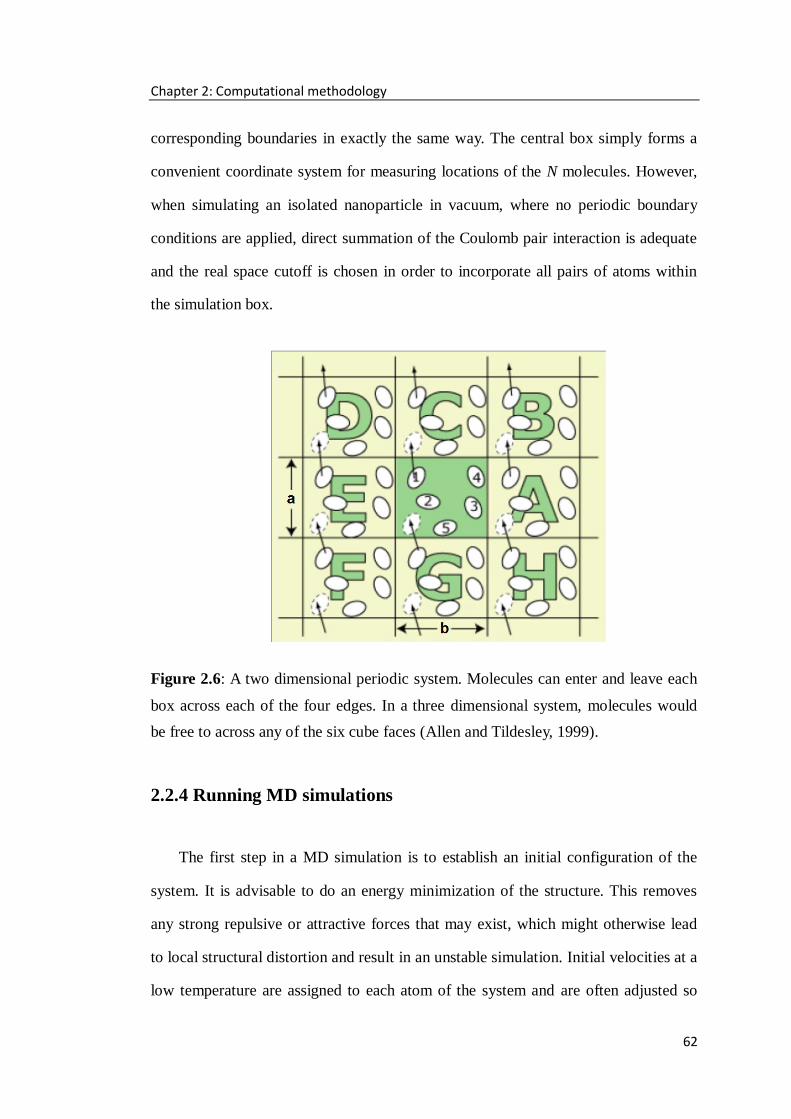
Chapter 2: Computational methodology
62
corresponding boundaries in exactly the same way. The central box simply forms a
convenient coordinate system for measuring locations of the N molecules. However,
when simulating an isolated nanoparticle in vacuum, where no periodic boundary
conditions are applied, direct summation of the Coulomb pair interaction is adequate
and the real space cutoff is chosen in order to incorporate all pairs of atoms within
the simulation box.
Figure 2.6: A two dimensional periodic system. Molecules can enter and leave each
box across each of the four edges. In a three dimensional system, molecules would
be free to across any of the six cube faces (Allen and Tildesley, 1999).
2.2.4 Running MD simulations
The first step in a MD simulation is to establish an initial configuration of the
system. It is advisable to do an energy minimization of the structure. This removes
any strong repulsive or attractive forces that may exist, which might otherwise lead
to local structural distortion and result in an unstable simulation. Initial velocities at a
low temperature are assigned to each atom of the system and are often adjusted so

Chapter 2: Computational methodology
63
that the total momentum of the system is zero, thus avoiding unnecessary
displacement of the whole system.
Having setup the system and assigned the initial velocities, the simulation can
commence. At each step the force on each atom must be calculated by differentiating
the potential functions. Newton‟s equations of motion are integrated to propagate the
system in time. Periodically, new velocities are assigned at a slightly higher
temperature and the simulation is allowed to continue. The initialization step is
terminated when the temperature stabilizes (the energy of the system is constant) and
no longer needs renormalization for this purpose because it has reached steady state.
The next step is to carry out the simulations in a given virtual time, which
contains a significant number of time steps Δt. In this process the positions and
velocities of the atoms in selected steps are recorded and stored. Generally, the MD
simulations are performed under conditions of constant number of atoms,
temperature and volume, but its trajectory can be modified to sample other
ensembles. Even in a constant NVE simulation it is usually desirable to perform a
simulation at a particular temperature and it is common practice during the
equilibration phase to adjust the temperature to the desired values.
When the system has achieved equilibrium, then the production phase can
commence. At the start of the production phase all counters are set to zero and the
system is allowed to evolve. In a micro-canonical ensemble (NVE) no velocity
scaling is performed during the simulation and the temperature becomes a calculated
property of the system. Various properties are routinely calculated and stored during
the production phase for subsequent analysis and processing. Careful monitoring of
these properties during the simulations can show whether the system is well behaved
or not. It may be necessary to restart a simulation if problems are encountered. It is

Chapter 2: Computational methodology
64
also usual to store the positions, forces and velocities at regular intervals, from which
other properties depending on these quantities can be determined at the end of the
simulation.
There are many available computer codes to run MD simulations depending on
the potentials used and the target applications. One of them is the DL_POLY code
(Smith and Forester, 1996), which is designed to facilitate MD simulations of
macromolecules, polymers, ionic systems and solutions on a distributed memory
parallel computer. DL_POLY allows almost any functional form of interatomic
potential to be used in the MD simulations. For the two-body terms, the standard
harmonic term is available as well as the Buckingham, Morse and Lennard-Jones
potential functions. It is also relatively easy to adapt forcefields from other libraries
to DL_POLY. The details of above interatomic potential functions will be discussed
in Chapter 3.
The integration algorithms in DL_POLY are based on the Verlet Leap-Frog
scheme discussed above, and the Nosé-Hoover algorithm is used for the thermostat,
as it can generate trajectories in both NVT and NPT ensembles, thus keeping the
simulations consistent. The thermostat parameters are set at 0.1 ps and the barostat
relaxation time is set at 0.5 ps. The simulations performed for this thesis are initially
performed using NVE and NVT ensembles to equilibrate the systems for a period,
and followed by both equilibration and the final data production run at NPT or NST
for another period of some time. A time step of 0.1 fs is applied to maintain the
stability of the simulations. The production phase produces a range of properties at
each time step, including structure, temperature, volume and energies. The energies
reported in the MD simulations in this thesis are the average configurational energies
obtained over each production phase, whereas the structures shown in the figures are
usually snapshots.

Chapter 2: Computational methodology
65
2.2.5 Analysis
The simplest way to analysis the results of the MD simulations is to visualise the
trajectory and animate the time evolution of the system. It is possible to observe the
growth and dissolution of crystals and phase transitions. Furthermore, a variety of
other properties can be calculated from the MD simulations, including
thermodynamic properties, radial distribution functions and diffusion coefficients.
The internal calculations in the simulation keep tracking of a number of
thermodynamic properties from which the instantaneous and ensemble average
values may be extracted. The total instantaneous potential energy for a time step is
calculated as the sum of the values from the evaluation of the interatomic potential
functions. Additionally, the instantaneous kinetic energy, at a time t, can be
calculated from the velocities of atoms in the system as
21( ) ( )
2
N
k i i
i
U t m v t (2.27)
where vi(t) is the velocity of an atom with the mass mi. This equation gives the
instantaneous kinetic energy and so the total energy is the sum of the potential and
kinetic energies. All of these quantities may be averaged over the length of the
simulation to give the ensemble averages or plotted with respect to time to observe
changes in the system.
The instantaneous temperature of the system is related to the kinetic energy of
the atoms. There is a contribution to Uk of kBT/2 for each degree of freedom in the
system, so for any time step the temperature becomes
2 ( )N
i i
i
B
m v t
Tk f
(2.28)

Chapter 2: Computational methodology
66
kB is the Boltzmann constant and f is the number of degrees of freedom. A complete
system is described by a maximum of 3N independent Cartesian coordinate degrees
of freedom (as an aside, each of these may be treated entirely independently in
calculations, enabling the calculations to be vectorised to increase speed).
Constraints and boundaries imposed on the system will reduce the number of degrees
of freedom.
The radial distribution function (RDF), g(r), is a useful measure of the
surroundings of an atom. For each atom type the distances to other atoms are sorted
into shells.
2
( ) 1( )
( ) 4
n rg r
r r r
(2.31)
where n(r) is the occupancy of a shell of width Δr at a radius r from the atom. The
factor of the mean atom density ρ(r), ensures that the distribution is normalized.
Values are averaged from all atoms in the sample and over each time step. For a fixed
ideal lattice, g(r) will be zero except at neighbour separation distances. At increased
finite temperatures the atomic vibrations cause movement away from these ideal
positions and the peaks in the function broaden.

67
3 Potential models
An interatomic potential model refers to a collection of parameters of
mathematical functions used to describe the interatomic interactions of a system. An
accurate potential model is essential to obtain reliable results. This chapter presents a
summary of the interatomic potential functions and parameters used in this thesis. In
addition, a new set of potential parameters for divalent cations Co2+
, Zn2+
, Mn2+
and
Ni2+
were derived with the existing calcite potential model. Details of the derivation
of these parameters are also presented in this chapter.
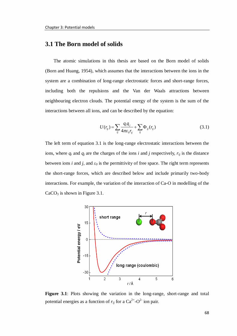
Chapter 3: Potential models
68
Po
ten
tial en
erg
y / e
V
3.1 The Born model of solids
The atomic simulations in this thesis are based on the Born model of solids
(Born and Huang, 1954), which assumes that the interactions between the ions in the
system are a combination of long-range electrostatic forces and short-range forces,
including both the repulsions and the Van der Waals attractions between
neighbouring electron clouds. The potential energy of the system is the sum of the
interactions between all ions, and can be described by the equation:
0
( ) ( )4
i j
ij ij ij
ij ijij
q qU r r
r (3.1)
The left term of equation 3.1 is the long-range electrostatic interactions between the
ions, where qi and qj are the charges of the ions i and j respectively, rij is the distance
between ions i and j, and ε0 is the permittivity of free space. The right term represents
the short-range forces, which are described below and include primarily two-body
interactions. For example, the variation of the interaction of Ca-O in modelling of the
CaCO3 is shown in Figure 3.1.
Figure 3.1: Plots showing the variation in the long-range, short-range and total
potential energies as a function of rij for a Ca2+
-O2-
ion pair.

Chapter 3: Potential models
69
Other contributions are also considered, such as bond bending terms to convey
the directionality of certain bonds in the crystal, for instance in the modelling of the
covalent bonds in the carbonate group of CaCO3, and four-body interactions such as
dihedral terms.
3.2 The Ewald method
The internal energy equation of the Born model seems deceptively simple.
However, the long-range electrostatic part of the potential energy is too slow to
converge as a function of rij in real-space. This problem has been solved by using the
Ewald summation method (Ewald, 1921), which replaces the summation of potential
energies in real space with an equivalent summation in Fourier space. The advantage
of this approach is the rapid convergence of the Fourier space summation compared
to its real-space equivalent when the real-space interactions are long-range. Because
it is maximally efficient to decompose the interaction potential into a short-range
component summed in real space and a long-range component summed in Fourier
space.
Each point charge in the system is viewed as being surrounded by a Gaussian
charge distribution of equal magnitude and opposite sign, with charge density:
32 2
3/ 2( ) exp( )i
i i i
qr r
(3.2)
where α is a positive parameter that determines the width of the distribution, and ri is
the position relative to the centre of distribution. This introduced charge distribution
screens the interaction between neighbouring point-charges, effectively limiting them
to a short range. Consequently, the sum over all charges and their images in real
space converges rapidly, which is now given by:
Chapter 3: Potential models
70
( )1
2
ij
sr i j
ij ij
erfc rU q q
r
(3.3)
where erfc(x) is defined as the complimentary error function:
2
0
2( ) 1 ( ) 1 exp( )
1/ 2
x
erfc x erf x u du
(3.4)
A second Gaussian charge distribution of the same sign and magnitude as the
original distribution is added in order to maintain the neutrality of charges. This time
the sum is performed in the Fourier space to solve the resulting Poisson's equation.
2
2, 0
exp[ ( / ) 2 ( )]1
2
i j
fr i j
i j m
m m r rU q q
V m
(3.5)
where m are the reciprocal vectors and V is the volume of the unit cell of the crystal.
A correction self-term needs to be subtracted in order to cancel out the interaction of
each of the introduced artificial counter-charges with itself. Finally, the total
electrostatic energy per unit cell can then be calculated as:
2
1/ 2ij sr fr i
i
U U q
(3.6)
3.3 Electronic polarisability
One simple way to include the electronic polarisability of the atoms is to use the
core-shell model (Dick and Overhauser, 1958), where the polarisable ion is
represented by a massless shell connected to a core containing all the mass. The total
charge of the ion is the sum of the charges of the core and shell. The position of the
core represents the position of the ion in the crystal lattice and the position of the
shell shows the electronic polarisability of the atom. The core and shell are connected
by a harmonic spring, as shown in Figure 3.2. The spring constant K and the charge

Chapter 3: Potential models
71
of the shell Ye then determine the polarisability of the ion as follows:
2
04p
Ye
K
(3.7)
Both K and Ye can be fitted empirically to reproduce experimental properties,
such as dielectric and elastic constants. The short-range forces are assumed to act
between the shells while the Coulombic forces act between all shells and cores,
except between the core and shell of the same ion. The core-shell model has been
successful in modelling various properties and it has been used in all static energy
minimisation calculations in this thesis to describe the polarisability of the oxygen in
the CO32-
group and water.
Figure 3.2: Schematic representation of the core-shell model: (a) no displacement,
unpolarised. (b) displacement, polarised. The blue sphere, representing the core, has
the charge Xe. The open grey sphere, representing the shell, has the charge of Ye. The
core and shell are connected by a spring of force constant K, (Murphy, 2009).
The core-shell model of electronic polarisability employed in MD simulations is
slightly different, because the massless shells do not obey the normal dynamic laws.
In DL_POLY, a small mass is assigned to the shell following the approach introduced
by Mitchell and Fincham (1993). For example, the oxygen shell in this thesis is given
a mass of 0.2 a.u., which is small enough, compared to the mass of hydrogen atom
(a) Unpolarised (b) Polarised
Chapter 3: Potential models
72
(1.0 a.u.), in order to minimise energy exchange between the vibrations of oxygen
core and shell and the oxygen and hydrogen vibrations. Due to the use of a shell
model, a time step of 0.1 fs is applied to maintain the stability of the simulations.
3.4 Short-range potential functions
The two-body potential functions act between neighbouring charge clouds, the
shells of the polarisable anions and the cores in the case of cations. They come in a
number of analytical forms, all describing the potential energy as a function of
interionic separation. These potential functions act without taking into account
directionality of any bonds. Three-body potential function acts between three ions
and is used when covalent bonds are present in the system. The terms define angles
and dihedrals between the ions and as such convey directionality to the bonds. The
short-range potential functions used in this thesis are described below.
3.4.1 Buckingham potential function
The Buckingham potential (Buckingham, 1938) is one of the most widely used
functions for the interaction of two bodies which are not directly bonded.
6( ) exp( )
ij ij
ij ij ij
ij ij
r Cr A
r (3.8)
where Aij, ρij and Cij are the parameters to describe the interaction between two atoms
i and j and rij is the interatomic distance. Aij and ρij are related to the number of
electrons and the electron density respectively. The first term of the function
describes the short-range repulsive interaction between the atoms, which originates
from the Pauli Exclusion Principle (1925), while the second represents the attractive
Van der Waals forces. Since the exponential term converges to a constant as the

Chapter 3: Potential models
73
distance rij approaches to zero, while the second term diverges, it runs the risk of an
un-physical “Buckingham catastrophe”, when used in simulations of charged
systems. This occurs when the electrostatic attraction artificially overcomes the
repulsive barrier (White, 1997). Minimizing the energy of a structure which
accidentally has a very short distance between two atoms will thus result in “nuclear
fusion”. Special precautions have to be taken to avoid this problem (Jensen, 2007).
Occasionally, the second term of the Buckingham potential used in this thesis is
omitted altogether and the Aij parameter is adjusted to take into account both the
long-range attractive forces and short-range repulsions.
3.4.2 Morse potential function
The Morse potential (Morse, 1929) is used for modelling covalent bonds and
capable of modelling anharmonicity. As such interatomic distances away from the
equilibrium bond distance can be simulated reliably with this potential function, for
example the carbon-oxygen bond in the CO32-
group.
0( ) 2( ) (1 e )ijr r
ij ij ijr D
(3.9)
where Dij is the depth of the potential well, i.e. the thermodynamic dissociation
energy of the bond, r0 is the equilibrium bond length, and α is a constant controlling
the “width” of the potential. The form of the Morse potential function ensures that at
infinite separation of the two atoms the potential energy is zero while the potential
energy is at a minimum at the equilibrium bond distance. Sometimes the Morse
potential is used with subtraction of the Coulombic interaction and as such it is the
only potential function describing a bond between two nearest neighbours.
Interactions between second and further nearest neighbours can be described by
Coulombic interactions and another short-range potential function.
Chapter 3: Potential models
74
3.4.3 Lennard-Jones potential function
The Lennard-Jones potential (Lennard-Jones, 1924), of which the commonest
form is also referred to as the 6-12 potential, is one of the most widely used potential
functions to approximate the interaction between a pair of atoms. It has the following
simplified form:
12 6(r )ij ij
ij ij
A B
r r (3.10)
with A = 4εσ12
and B = 4εσ6, where ε is the depth of the potential well and σ is the
finite distance where the inter-particle potential is zero. The repulsive part is
dependent on r-12
and thus acts at close range, while the attractive part is proportional
to r-6
and becomes dominant at longer range. The parameters can be fitted to
reproduce experimental data or accurate quantum chemistry calculations. Due to its
computational simplicity, the Lennard-Jones potential is used extensively in
computer simulations even though more accurate potentials exist. For example, it is
often used for modelling oxygen-oxygen interactions in water potential models, such
as the SCP and TIP5P models (Jorgensen et al., 1983; Rick, 2004).
3.4.4 Many body potential function
The three-body harmonic potential is used to describe the partial covalency in
the CO32-
group and maintain the bond angle between two carbon-oxygen bonds.
2
0
1( ) ( )
2ijk i jk ijk ijkk (3.11)
where kijk is the force constant and (θijk-θ0) is the deviation from the equilibrium
angle θ0. The function acts between a central ion i and two ions j and k bonded to i
making the bond angle θijk (see Figure 3.3).

Chapter 3: Potential models
75
Figure 3.3: The three-body interaction in a carbonate group.
The four-body out of plane potential is applied to planar arrangements of three
bonds or torsional angles (Figure 3.4). The four-body potential function for the CO32-
group is described as follows by Pavese et al. (1996).
[1 cos( )]ijkl ijklk s N (3.12)
where kijkl is the force constant, s is ±1 and N is an integer which gives the periodicity
of the torsion, which is 2 in the case of the planar CO32-
group. The above functional
form means that the energy has a minimum vale when θ is 0 or π radians and all
atoms lie in the same plane in the CO32-
group.
Figure 3.4: The four-body interaction of four atoms lying in two planes with a
torsional angle θ.
j
i
k
θijk
Chapter 3: Potential models
76
3.5 Potentials of carbonates and water
The potential parameters of calcite used in this thesis are from Pavese et al.
(1996), who derived them empirically in a study of the thermal dependence of
structural and elastic properties of calcite. The oxygen-oxygen and calcium-oxygen
interactions are modelled by a Buckingham potential. The covalency within the
CO32-
group is modelled by a Morse potential plus a three-body potential and a
torsional potential function to restrain the planar CO32-
group from folding. Although
Pavese et al.‟s potential model was fitted to bulk structure; it has been applied
successfully to the accurate representations of calcite surfaces (de Leeuw and Parker,
1998, 2000, 2001). The potential parameters used for CdCO3, MgCO3 and FeCO3
were derived by de Leeuw (2002), which were fitted to reproduce the unit cell
volumes of relative carbonates with respect to calcite, as well as relative energies of
formation of these carbonates, using on the same potential parameters of CO32-
group.
The water potential model is that of de Leeuw and Parker (1998) with the added
hydrogen-bonding modification of Kerisit and Parker (2004). For the interactions
between water and calcite, the potential parameters come from de Leeuw et al.
(1999). The potential parameters used in the thesis are summarised in Table 3.1.

Chapter 3: Potential models
77
Table 3.1 Potential parameters used in this thesis (short-range cutoff 20 Å).
(Parameters for CaCO3 are from Pavese et al., 1996; Parameters for Mg, Fe, Cd are
from de Leeuw, 2002; parameters for water are from de Leeuw and Parker, 1998 and
Kerisit and Parker, 2004).
ions Charge core-shell
Interaction / eVÅ-2
core shell
Ca, Mg, Fe, Cd +2
C +1.135
H +0.400
O +0.587 -1.632 507.4
Owater +1.250 -2.050 209.449602
Buckingham Potential
Ion pair A / eV ρ / Å C / eVÅ6
Ca-O 1550.0 0.297 0.0
Mg-O 1092.2 0.27926 0.0
Fe-O 14600.0 0.2055 0.0
Cd-O 747097.4 0.1549 0.0
Ca-Owater 1186.6 0.297 0.0
H-O 396.3 0.23 0.0
H-Owater 396.3 0.25 10.0
O-O 16732.0 0.213 3.47
O-Owater 12533.6 0.213 12.09
Lennard-Jones Potential
A / eVÅ12
B / eVÅ6
Owater-Owater 39344.98 42.15
Morse Potential
D / eV α / Å-1
R0 / Å
C-Ocore 4.71 3.8 1.18
H-Owater-shell 6.203713 2.22003 0.92376
Three Body Potential
k / eVrad-2
Θ0
Ocore-C-Ocore 1.69000 120.0
H-Owater-shell-H 4.19978 108.69
Four Body Potential
k / eVrad-2
Θ0
C-Ocore-Ocore-Ocore 0.11290 180.0

Chapter 3: Potential models
78
3.6 Derivation of potentials for Ni, Co, Zn and Mn carbonates
There are two ways to derive the potential parameters for the short-range
potential functions. One is a non-empirical method which is based on ab initio
calculations to obtain the data for the parameterization, such as the equilibrium
geometry and the energy surface corresponding to a particular structural distortion.
The other is an empirical method which determines the parameters of the pair
potential functions to reproduce specific experimental properties, such as
crystallographic data, unit cell dimensions and elastic constants. The empirical
method often produces a series of values, which can repeat the lattice parameters for
a given structure. However, it is much more desirable and accurate to consult as
many observable properties as possible.
The potential parameters for NiCO3, CoCO3, ZnCO3 and MnCO3 in this thesis
were derived using GULP (Gale, 1997) by a penalty minimisation scheme. In this
scheme, the total penalty of a system is the sum of the deviations of calculated
properties, such as atomic positions or elastic parameters, from measured values
weighted according to accuracy. During fitting, the parameters of the interatomic
potentials are adjusted so as to minimize the penalty value of the system until it has
converged. The following options were used when fitting the potential parameters in
GULP. (i) Constant pressure and relaxed fitting algorithm where both cores and
shells of ions are allowed to move within the cell during fitting. (ii) Newton-Raphson
algorithm was applied during energy optimisation. (iii) Parameters were generally
fitted one at a time, except where a material had a well-defined structure and known
elastic constants.
The primitive rhombohedral cell was used in the simulation of the bulk structure
of calcite-type carbonates, although lattice parameters are reported here in hexagonal

Chapter 3: Potential models
79
coordinates as the two representations are mathematically equivalent. The potential
parameters for NiCO3, CoCO3, ZnCO3 and MnCO3 were derived by GULP to be
compatible with the potential model of calcite by Pavese et al., where the calculated
hexagonal unit cell volume is 348.3 Å3 (a = 4.797 Å, c = 17.482 Å, α = 90
o and γ =
120o). During fitting, the potentials were required to retain the relative hexagonal
unit cell volumes in the experimental ratio:
: : : : 1.34 :1.12 :1.02 :1.02 :1Ca Mn Co Zn NiV V V V V (3.13)
The only degree of freedom allowed in fitting the potentials was in the
cation-oxygen Buckingham potential. Due to the non-directional natural of the metal
cation as described by the Buckingham potential of equation 3.8, there is no explicit
term that addresses the d-electrons of the transition metal cations. The transition
metal cations are represented as spherical rigid ions with no electronic polarization,
as in Ca2+
, and therefore magnetic effects are ignored. Fortunately, magnetism is
unlikely to affect the issues, such as the enthalpy and free energy of mixing, which
are interested in exploring in this thesis.
In order to obtain the reliable enthalpies for cation substitutions, the relative
enthalpies of formation are required to be sensible. Therefore the enthalpy of the
following reaction is required to be reproduced accurately:
2 2
( ) 3( ) ( ) 3( )g s g sCa MeCO Me CaCO (3.14)
where Me is Ni, Co, Zn or Mn. The potential parameters were therefore derived such
that the calculated enthalpies of reaction 3.14 agree to within 2.2% of the
experimental enthalpies. In this calculation the vibrational effects (both zero-point
and heat capacity) were included in the enthalpies, although they contribute very
little to the reaction enthalpy, for example, only 1.3 kJ/mol (0.5%) of the reaction

Chapter 3: Potential models
80
enthalpy for MnCO3. Table 3.2 provides the optimized interatomic potential
parameters of these four carbonates obtained through this process, and a comparison
of calculated and experimental parameters for the various carbonates is listed in
Table 3.3.
Table 3.2 Interionic Buckingham potentials obtained from fits to NiCO3, CoCO3,
MnCO3 and ZnCO3 structures and enthalpies of reaction 3.14.
Ion pair A / eV ρ / Å C / eVÅ6
Ni-O 1103.38 0.26661 0.0
Co-O 1561.50 0.26740 0.0
Mn-O 1704.60 0.27400 0.0
Zn-O 1506.62 0.26903 0.0
No interatomic potential model is perfect, and usually the description of some
properties can only be improved at the expense of worsening the description of
others. For example, the parameters of Buckingham potential for Co2+
and Zn2+
introduced in this thesis are less well reproduced the experimental bulk modulus, and
the calculated bulk modulus of ZnCO3 is bigger than that of CoCO3, which is
contradict with experiments. However, both the ratio of the cell parameters and
calculated enthalpies of reaction 3.14 are reproduced very well, therefore these
parameters should provide an adequate description of the incorporation of single kind
of cationic impurity in calcite.

Chapter 3: Potential models
81
Table 3.3 Calculated and experimental properties of NiCO3, CoCO3, ZnCO3, MnCO3
and CaCO3. (Experimental lattice parameters are from Deer et al., 1992; bulk
modulus are from Zhang and Reeder, 1999; the enthalpies of formation of carbonates
are from Lide, 2000).
Carbonates Volume
/Å3
a / Å c / Å c/a
Bulk
modulus
/ GPa
ΔHEq-3.14
/ kJmol-1
CaCO3 experiment 367.8 4.99 17.06 3.42 76.1 /
literature 348.3 4.80 17.48 3.64 80.4 /
ZnCO3 experiment 281.01 4.67 14.88 3.19 123 462.5
this work 264.42 4.46 15.35 3.44 216 454.4
CoCO3 experiment 281.22 4.67 14.89 3.18 124 426.7
this work 269.07 4.48 15.48 3.46 213 416.3
MnCO3 experiment 307.89 4.78 15.56 3.26 126 279.3
this work 285.24 4.55 15.91 3.49 135 275.2
NiCO3 experiment 274.65 4.64 14.73 3.17 131 440.2
this work 236.25 4.33 14.55 3.36 150 432.9

82
4 Mixing thermodynamics of calcite with
divalent cation impurities
In this chapter atomistic simulation techniques have been employed to
investigate the thermodynamics of mixing calcite with divalent cation impurities
Me2+
(Cd2+
, Mn2+
, Fe2+
, Co2+
, Zn2+
, Mg2+
and Ni2+
), based on the calculation of all
inequivalent site occupancy configurations in relevant supercells of calcite structure.
The simulations predict that the miscibility of calcite and other carbonates is largely
related to the cationic coordination distance with oxygen. Detailed comparisons of
the simulations with available experimental results are also provided in this chapter.
Chapter 4: Mixing thermodynamics of calcite with divalent cation impurities
83
4.1 Introduction
Metal cations, such as Cd2+
, Mn2+
, Zn2+
, Fe2+
, Co2+
Ni2+
and Mg2+
, are
commonly present in calcite, which can take up the impurity cations via a dissolution
recrystallisation process. The solubility and migration of divalent cations in calcite is
largely limited by the phase equilibrium of two carbonates, many of which form
calcite-type solid solutions. For example, studies by Tesoriero and Pankow (1996)
showed that in the presence of calcite, precipitation of Cd2+
as a carbonate solid
solution will always occur, even when Cd2+
is present at trace levels, due to the
strong tendency of this cation to partition into calcite. It is therefore very useful to
investigate the thermodynamics of these extensive solid solutions to gain insight into
the flux of divalent cations in aquifers and soil.
Although the mixed carbonate solid solutions have been widely studied using
experimental techniques, such as solution calorimetry, seemingly contradictory
results are still reported in the literature, particularly with respect to the range of the
miscibility at different temperatures and the thermodynamics of the mixing
properties at intermediate compositions, since the slow kinetic rate at high
temperatures and pressure limits further progress in experiments. One of the most
straightforward theoretical models for predicting the thermodynamics of binary
carbonate solid solutions is the electrostatic model from Lippmann (1980). However,
some assumptions in this model limit its power of prediction. For example,
Lippmann‟s model assumes all calcite-type carbonates should have the same
Madelung constant.
As an effective complementary technique to experiment, computer modelling
can be used to study complex mineral structures and processes at the atomic level,

Chapter 4: Mixing thermodynamics of calcite with divalent cation impurities
84
including the formation of solid solutions, where it is possible to access the
thermodynamic properties without the effect of unknown kinetic factors. Interatomic
potential models, in particular, have been used extensively to simulate the structures
and properties of rhombohedral carbonates (Cygan, 2000; de Leeuw and Parker,
1996, 1997; Austen, 2005). These studies have demonstrated the suitability of
molecular simulations in providing a theoretical description of complex bulk and
surface processes in carbonates, and how the theoretical models assist experiment in
the evaluation and interpretation of experimental observations.
For a carbonate solid solution, the number of possible configurations for each
composition increases rapidly with the size of the simulation supercell, leading to
concomitant computational cost. Several approaches have been developed to treat
these large numbers of configurations. For example, the thermodynamics of the
binary (Mn,Ca)CO3 system and tertiary (Mg,Mn,Ca)CO3 system have been discussed
in recent papers by Vinograd et al. (2009 and 2010), where a simplified pair-wise
interaction model is employed to perform Monte Carlo simulations in a very large
supercell of the structure, allowing full convergence of the calculations with respect
to cell size. An alternative approach, which has been adopted in this study, is to
reduce the complete set of configurations to the symmetrically inequivalent
configurations by taking advantage of the crystal symmetry of calcite. This method
keeps an accurate description of the interatomic interactions and relaxation effects
explicitly in the simulations, based on the calculation of all inequivalent site
occupancy configurations in a smaller supercell of the calcite structure. It also makes
possible to calculate effective properties, beyond the energy, based on
configurational averages (for example, effective cell parameters as a function of
composition), and to evaluate easily the contribution of vibrational effects.

Chapter 4: Mixing thermodynamics of calcite with divalent cation impurities
85
In this chapter atomistic simulation techniques have been applied to investigate
the thermodynamic properties of the entire compositional range of a series of binary
carbonate solid solutions (Me,Ca)CO3 (Me = Cd2+
, Mn2+
, Zn2+
, Fe2+
, Co2+
, Ni2+
,
Mg2+
), following the above approach. In addition to the enthalpy of mixing, the
calculation of the configurational entropy and free energy has also been included;
therefore it is possible to study the mixing behaviour as a function of temperatures
for these binary carbonate solid solutions. The results were then compared with
experimental measurements from calorimetric methods.
4.2 Configurational statistics
The distribution of cationic impurities in the hexagonal calcite lattice was
investigated utilizing the SOD (Site Occupancy Disorder) program (Grau-Crespo,
2007), which generates the complete configurational space for each composition of
one supercell and then extracts the symmetrically inequivalent configurations by
considering the symmetry operators of the parent structure. Typically this procedure
significantly reduces the number of configurations to be calculated in the GULP code
(Gale, 1997). Once the configurational spectrum is obtained, it is possible to derive
configurational entropies and enthalpies, based on the assumption that the extent of
the occurrence of one particular configuration in the disordered solid can be
described by a Boltzmann-like probability which is calculated, assuming zero
external pressure and ignoring vibrational contributions, from the energy Um of the
configuration (the minimum energy of the optimised structure at constant pressure),
and its degeneracy Ωm (the number of times that the configuration is repeated in the
complete configurational space):
exp( / )mm m BP U k T
Z
(4.1)

Chapter 4: Mixing thermodynamics of calcite with divalent cation impurities
86
where m = 1, …, M (M is the number of inequivalent configurations), kB =
8.6173×10⁻⁵
eVK-1
is the Boltzmann‟s constant, and Z is the configurational partition
function.
1
exp( / )M
m m B
m
Z U k T
(4.2)
In this study, the enthalpy of each configuration is simply its lattice energy, as
any external pressure has not been considered in the calculations, and the vibrational
contributions to the enthalpy have been ignored, which were shown in a previous
study on (Fe,Cr)2O3 solid solution to be negligible (Benny et al., 2009). Then the
enthalpy per formula H at each composition is calculated as an average in the
configurational space:
1 1
1 1M M
m m m m
m m
H P H P UN N
(4.3)
where N is the number of formula units in the supercell, while the configurational
free energy G and the entropy S can be obtained from the partition function Z:
1lnB
NG k T Z ; (4.4)
1
1ln
Mm
B m
m m
PH GS k P
T N
. (4.5)
It is worth noting that the calculated enthalpies of the disordered systems tend to
converge very rapidly with the size of the simulation cell, although the convergence
of entropies is much slower (Todorov, 2004). Therefore, the calculations, which are
based on relatively small supercells, can provide precise enthalpies, while the
calculated entropies are only used to qualitatively access the degree of disorder in the
solid solutions. The degree of convergence of the entropies with the size of the
supercell is discussed below based on the difference between the full-disorder

Chapter 4: Mixing thermodynamics of calcite with divalent cation impurities
87
entropy for the given supercell:
max
1 !( , ) ln
[ ]![ (1 )]!B
NS x N k
N Nx N x
. (4.6)
and the exact full-disorder result:
max( ) lim ( , ) [ ln (1 ) ln(1 )]ideal BN
S x S x N k x x x x
. (4.7)
Any property Am defined for each configuration m can be averaged over the
configurational ensemble as:
1
M
m m
m
A P A
(4.8)
But the interpretation of this average should be done carefully. When the averaging
of system properties is performed in the reduced space of inequivalent configurations,
each configuration m represents a set of Ωm equivalent configurations, and therefore
the property Am must be the same for all configurations in that set. For example, if am
and bm are the equilibrium cell vectors for each inequivalent configuration m, the
average value of the cell parameters a corresponding to the disordered crystal cannot
be calculated as the direct average of the |am| values, as this result could be different
from the direct average of the |bm| values, breaking the rotational symmetry of the
hexagonal cell. Therefore we have calculated the cell parameter a by equation:
1
2
1
( )M
m m m
m
a P
a b (4.9)
Since the absolute value of the vector product am×bm is invariant within a set of
equivalent configurations. The cell parameter c was obtained directly by
configurational averaging of the |cm| values.

Chapter 4: Mixing thermodynamics of calcite with divalent cation impurities
88
In order to interpret the thermodynamic properties of the binary solid solutions
in an appropriate way, the size of the simulation cell in the calculations must be
clarified. The cation substitutions in 2 × 2 × 1 and 3 × 3 × 1 supercells have been
considered, which contain 24 and 54 cation sites respectively. The extension along
the x/y-axes is studied, as a < c in the unit cell and the interactions of cations in
neighbouring cells thus could have more effect in x/y-axes. The total number of
configurations and symmetrically inequivalent configurations for two supercells are
listed in Table 4.1, where x is the molar fraction of the impurity cations in the solid
solutions.
Table 4.1 Total number of configurations (W) and number of symmetrically
inequivalent configurations (M) for each composition MexCa1-xCO3 in 2 × 2 × 1 and
3 × 3 × 1 supercells (A and B stand for either Ca or impurity).
Cell composition x or 1-x W M
A24(CO3)24 0 1 1
A23B(CO3)24 0.042 24 1
A22B2(CO3)24 0.083 276 7
A21B3(CO3)24 0.125 2024 20
A20B4(CO3)24 0.167 10626 102
A19B5(CO3)24 0.208 42504 317
A18B6(CO3)24 0.250 134596 1033
A17B7(CO3)24 0.292 346104 2467
A16B8(CO3)24 0.333 735471 5330
A53B(CO3)54 0.019 54 1
A52B2(CO3)54 0.037 1431 11
A51B3(CO3)54 0.056 24804 86
A50B4(CO3)54 0.074 316251 1051

Chapter 4: Mixing thermodynamics of calcite with divalent cation impurities
89
For the 2 × 2 × 1 supercell, the full spectrum of configurations was not
calculated for Me2+
composition 0.333 < x < 0.667 due to the still prohibitive
computational cost. For example, for the intermediate composition x = 0.5, it leads to
a total of almost three million configurations, which is computationally too
expensive to calculate directly. Instead, a random sampling method was employed
and the convergence of the calculated properties with respect to the sample size was
checked. The 3 × 3 × 1 supercell was only employed at low concentrations to test the
convergence of enthalpies with respect to cell size.
4.3 Structure and configurational entropy
Firstly, the equilibrium geometries and energies of the divalent cation substituted
configurations in a 2 × 2 × 1 supercell of the calcite structure were calculated using
the methods above. As calcite and other rhombohedral carbonate minerals are
iso-structural, the introduction of impurity cations in either material does not
significantly affect the structure beyond local relaxations.
In order to understand the driving force towards the cationic ordering in the
calcite-type structure, the most stable (lowest energy) configuration has been
identified. Figure 4.1 shows the lowest-energy configurations for x = 0.167, x =
0.333 and x = 0.5. A clear pattern emerges here: cationic dopants prefer to
concentrate on the same layer perpendicular to the hexagonal cell main axis (c-axis),
and at the same time, these full impurity layers prefer to be as far as possible from
each other. These ordered patterns are consistent with a simple interaction model
where Mn2+
-Mn2+
interactions are favourable within (0001) planes but unfavourable
between planes, as suggested recently by Katsikopoulos et al. (2009) based on
empirical evidence. This tendency is quite strong and remains valid for all

Chapter 4: Mixing thermodynamics of calcite with divalent cation impurities
90
compositions in the solid solutions, as will be discussed below.
(a) (b) (c)
Figure 4.1: The structures of the most stable configurations for x = n/6 (n = 1, 2, 3).
The lowest-energy structures for n = 4 and 5 can be obtained from the ones with n =
2 and 1, respectively, if Ca2+
and impurity Me2+
positions are swapped. The n = 3
case (x = 0.5) corresponds to the ordered dolomite-type structure. (Ca = green, C =
grey, O = red, Me = blue).
Figure 4.2 shows the calculated lattice energy Um of the mixed systems for Me
composition x = 0.25, where the black line is the lowest lattice energy, the blue line is
the highest lattice energy, and the red line is the average in the complete
configurational space for this composition. A simple inspection of the results shows
that the difference between the lowest and highest lattice energies Um generally
declines with increasing Me-O coordination distance, namely ΔUNi > ΔUMg > ΔUZn >
ΔUCo > ΔUFe > ΔUMn > ΔUCd. For the mixed carbonate system containing either Ni2+
,
Mg2+
, Zn2+
, Co2+
or Fe2+
, the average lattice energy approximately equals the lowest
lattice energy; therefore a large degree of cation ordering should be expected in these
systems, at least when temperature is not included in the calculations.
c
a

Chapter 4: Mixing thermodynamics of calcite with divalent cation impurities
91
Figure 4.2: The lowest (black line) and highest (blue line) lattice energies of mixed
systems for Me2+
composition x = 0.25, compared to the average lattice energy in the
configurational space (red line).
Figure 4.3: Configurational spectrum of lattice energies corresponding to the
composition of Cd0.25Ca0.75CO3 at 300 K, as calculated in a 2 × 2 × 1 supercell.
0.000 0.003 0.006 0.009
0.0
0.1
0.2
0.3
0.4
0.5
0.6
0.7
0.8
Um
/ K
Jm
ol-1
Pm
-251.0
-250.5
-250.0
-249.5
-249.0
-248.5
-248.0
Cd2+
Mn2+
Fe2+
Zn2+
Co2+
Mg2+
Ni2+
Um
/ k
Jm
ol-1

Chapter 4: Mixing thermodynamics of calcite with divalent cation impurities
92
On the contrary, there should be a certain degree of cationic ordering in the cases
of Mn2+
or Cd2+
. The spectrum of configurations corresponding to Cd2+
composition
x = 0.25 at 300 K is shown in Figure 4.3, where the zero-level (ground state) is
defined as the lattice energy of the most stable configuration. The number of
configurations with more homogeneous Cd2+
distribution is larger than those with
cation ordering, and the entropic effect is much stronger than the weak stabilization
yielded by the interaction between the impurities. Thus a great deal of cation disorder
should be present in the Cd2+
distribution at moderate temperatures.
The configurational entropy provides a quantitative measure of the degree of
cation ordering in the mixed systems. As the impurity cation composition x = 0.042
corresponds to one Me2+
substitution of any of the 24 equivalent Ca2+
in a 2 × 2 × 1
supercell, all 24 configurations are therefore equivalent and the configurational
entropy remains at its maximum value, Smax, for this supercell with an increase in
temperature. For other impurity compositions, where there are a number of possible
inequivalent distributions of the cations, the configurational entropy is not constant
and gradually approaches the maximum value at high temperatures. Figure 4.4 shows
the variation of the configurational entropy of the solid solutions with temperatures
at Me2+
composition x = 0.333. For Cd2+
, the entropy curve quickly reaches 96% of
its maximum value at 300 K, and 98% at 700 K, which means the solid solution is
almost ideally disordered even at relatively low temperatures of around 300 K. For
Mn2+
, the configurational entropy reaches 16% of its maximum value at 300 K, and
74% at 1000 K, indicating that some level of ordering can be present at low
temperatures (<1000 K), if there is full configurational equilibrium. For other cations,
Ni2+
, Mg2+
, Zn2+
, Co2+
and Fe2+
, the configurational entropy deviates from its
maximum value even at relevant high temperature (e.g. ~1900 K), which means that
a great deal of cation ordering should be expected in these solid solutions.

Chapter 4: Mixing thermodynamics of calcite with divalent cation impurities
93
Figure 4.4: Variation of the configurational entropy corresponding to the
composition of Me0.33Ca0.67CO3 at 300 K, as calculated in a 2 × 2 × 1 supercell.
Figure 4.5: Variation of the maximum configurational entropy (in the full disorder
limit) with the supercell size.
It is important to note here that the absolute entropy values are not well
converged with respect to the supercell size 2 × 2 × 1 for N = 24. To illustrate this
300 700 1100 1500 19000
1
2
3
4
5
6
7
S /
JK
-1m
ol-1
Temperature / K
Ni2+
Mg2+
Zn2+
Co2+
Fe2+
Mn2+
Cd2+
0.0 0.2 0.4 0.6 0.8 1.0
0
1
2
3
4
5
6
Infinite cell
3 x 3 x 1 cell (N=54)
2 x 2 x 1 cell (N=24)
1 x 1 x 1 cell (N=6)
Sm
ax(x
,N)
/ J
K-1
mo
l-1
x in MexCa
1-xCO
3

Chapter 4: Mixing thermodynamics of calcite with divalent cation impurities
94
point, the variation of the maximum entropy Smax for different cell sizes in
comparison with the exact results in the full disorder limit, for which an analytical
expression exists (equation 4.7), is shown in Figure 4.5. For the 2 × 2 × 1 supercell
(N = 24) the high temperature limit is in significant error (e.g. by 12% for x = 0.25).
Although the calculated configurational entropies are not fully converged, they are
still useful to assess the level of order to be expected in the systems.
4.4 MnCO3-CaCO3 solid solutions
Manganese carbonate (MnCO3) occurs naturally as the mineral rhodochrosite,
which is iso-structural with calcite. The significant difference in ionic radius between
Ca2+
(1.00 Å) and Mn2+
(0.83 Å) for six-fold coordination suggests that a fully
disordered solution is unlikely to occur in the mixed carbonate. The variation of the
configurational entropy of the (Mn,Ca)CO3 system with temperature also indicates
that a random distribution of Mn2+
can only be present in calcite at high temperatures,
as we have discussed before.
Although (Mn,Ca)CO3 solid solutions have been widely studied using
experimental techniques, seemingly contradictory results are still reported in the
literature, particularly in respect of the range of the miscibility gap at different
temperatures and the thermodynamics of the mixing properties at intermediate
compositions. Several researchers have proposed the existence of a wide miscibility
gap in the MnxCa1-xCO3 solid solution. For example, Goldsmith and Graf (1957)
reported the existence of a miscibility gap for 0.6 < x < 0.75 at ambient temperatures,
and suggested that complete miscibility only occurs above 823 K. De Capitani and
Peters (1981) studied the solvus in the (Mn,Ca)CO3 system and found that the critical
point lies at 813 K with a miscibility gap for 0.5 < x < 0.9 at 623 K. In contrast, other

Chapter 4: Mixing thermodynamics of calcite with divalent cation impurities
95
studies that have analyzed samples of natural and synthetic origin, have found that
the miscibility gap covers most of the Mn2+
compositional range at room temperature
(Winter et al., 1981; Pedersen, 1982; McBeath et al., 1998).
The intermediate composition Mn0.5Ca0.5CO3 and the stability of the ordered
phase with this composition (kutnahorite) at different temperatures also leave a
number of unanswered questions. For example, Capobianco and Navrotsky (1987)
reported a positive free energy of mixing for the Mn0.5Ca0.5CO3 system at high
temperature. Similarly, Katsikopoulos et al. (2009) also determined from
calorimetric measurements a positive enthalpy of mixing for the Mn0.5Ca0.5CO3
system at 298 K, although McBeach and co-workers (1998) measured a negative
value at 298 K. Furthermore, whereas the ordered kutnahorite structure has been
found in previous work, Katsikopoulos et al. (2009) indicated that it is not likely to
precipitate at ambient temperatures, and the X-ray diffraction experiments do not
show the clear superstructure reflections typical of kutnahorite ordering. They argue
that these incompatible results are probably due to kinetic factors, such as
precipitation rate and phase equilibrium at high supersaturation, which are difficult to
control in experiments.
In order to study the thermodynamic stabilities of the solid solutions, including
the contribution from the configurational entropy, it is useful to evaluate the enthalpy
of mixing and free energy of mixing as a function of composition at a range of
temperatures:
1 3 3 3
1 1[ ] (1 ) [ ] [ ]mix x xH H Mn Ca CO x U CaCO x U MnCO
N N (4.10)
1 3 3 3
1 1[ ] (1 ) [ ] [ ]mix x xG G Mn Ca CO x U CaCO x U MnCO
N N (4.11)
where H[MnxCa1-xCO3] is the enthalpy per formula unit of the solid solution,

Chapter 4: Mixing thermodynamics of calcite with divalent cation impurities
96
G[Ca1-xMnxCO3] is the free energy per formula unit of the mixed system, and
U[CaCO3] and U[MnCO3] are the lattice energies of the pure calcite and
rhodochrosite, as there are no configurational entropy contributions to the free
energy of the pure carbonate systems.
The negligible errors associated with using the internal energies U (instead of
the proper enthalpies H, which include both zero-point and heat capacity
contributions) have been found. For example, for Mn1/24Ca23/24CO3 at 298 K, the
enthalpy of mixing changes from ∆Hmix = 0.707 kJmol-1
to 0.699 kJmol-1
when
vibrational contributions are considered, which is change of ~1% only. This is not
surprising, as vibrational contributions to mixing enthalpies tend to be very small
(Benny et al., 2009; Ruiz-Hernandez et al., 2010). This simplification is a significant
advantage to the simulation, as the free energy minimisation costs much more
computational time and requires a separate set of energy minimisation at each
temperature. Conversely, the same set of configuration energies can be used for the
statistics at any temperature if the vibrational contribution is ignored.
At first the fully disordered MnxCa1-xCO3 system for compositions x < 0.33 was
investigated. All the equilibrium geometries and energies of the Ca-rich
configurations were calculated, and the average energy was taken in the high
temperature limit (T→∞), i.e., configurations were only weighted by their
degeneracies, regardless of their energies. Figure 4.6 shows the enthalpies of mixing
ΔHmix as a function of Mn2+
composition, together with experimental findings by
other authors. The calculated ΔHmix of the fully disordered system is clearly positive,
which is also seen in experiments. The consideration of a larger simulation cell (3 ×
3 × 1, red empty squares in Figure 4.6), does not seem to alter significantly the
values of the mixing enthalpy. However, the theoretical values seem to be too high

Chapter 4: Mixing thermodynamics of calcite with divalent cation impurities
97
when compared with the calorimetric measurements by Katsikopoulos et al. (2009)
and Capobianco & Navrotsky (1987).
Figure 4.6: Calculated and experimental mixing enthalpies for the Ca-rich
MnxCa1-xCO3 solid solution. The empty squares in red colour correspond to
calculations in the full disorder limit with the 3 × 3 × 1 supercell.
This discrepancy can arise from systematic errors in either the simulations or the
experiments. However, it is also possible to explain this discrepancy by considering
that there may be some degree of ordering in the experimental samples, which
reduces their mixing enthalpies with respect to the full disorder limit. It is notable
that although Katsikopoulos et al. (2009) were able to rule out kutnahorite type (see
Figure 4.1c) of ordering in their samples, based on the absence of superstructure
reflections in the X-ray diffraction (XRD) patterns, diffraction techniques are not
well suited to assess the level of disorder in poorly ordered samples, say, in
comparison with the ideal disorder limit. Therefore, the suggestion of imperfect
disorder in the samples does not conflict with the available experimental information.
Figure 4.6 also illustrates the enthalpies of mixing for the calcium-rich mixed system
0.0 0.1 0.2 0.3 0.4-1
0
1
2
3
4
5
6
Katsikopoulos et al. (2009) (T=298 K)
Capobianco & Navrotsky (1987) (T=873 K)
Theory- Full disorder (TeffInfinity )
Theory- Partial disorder (Teff
=1000 K)
Theory- Partial disorder (Teff
=300 K)
x in MnxCa
1-xCO
3
H
mix /
kJ
mo
l-1

Chapter 4: Mixing thermodynamics of calcite with divalent cation impurities
98
considering full equilibration at 300 K and 1000 K. The theoretical values of ΔHmix
of the partially ordered systems are lower as a result of higher weighting of the
lower-energy configurations. In this case, the theoretical prediction agrees much
better with the experimental results, especially when considering the wide error bars
of the experimental data points.
Figure 4.7: Calculated and experimental mixing enthalpies for the Mn-rich
MnxCa1-xCO3 solid solution. The empty squares in red colour correspond to
calculations in the full disorder limit with the 3 × 3 × 1 supercell.
Similar trends of mixing enthalpies were also found in the case of Ca-substituted
rhodochrosite, i.e. MnxCa1-xCO3 solid solutions with high concentrations of Mn2+
.
Figure 4.7 shows the enthalpies of mixing as a function of Mn2+
composition (x >
0.66), again compared with experiments. As for the Ca-rich compositions, the
consideration of a larger 3 × 3 × 1 supercell does not change significantly the values
of the mixing enthalpies. The ΔHmix for the incorporation of Ca2+
in rhodochrosite is
somewhat higher than for Mn2+
impurities in calcite, i.e. it is energetically more
0.6 0.7 0.8 0.9 1.0-4
-2
0
2
4
6
8
x in MnxCa
1-xCO
3
H
mix /
kJ
mo
l-1
Katsikopoulos et al. (2009) (T=298K)
Capobianco & Navrotsky (1987) (T=873K)
Theory- Full disorder (Teff Infinity)
Theory- Partial disorder (Teff=1000K)
Theory- Partial disorder (Teff=300K)

Chapter 4: Mixing thermodynamics of calcite with divalent cation impurities
99
expensive to substitute Ca2+
into rhodochrosite than Mn2+
into calcite, due to the
larger ionic radius of Ca2+
compared to Mn2+
. It is generally found that smaller
cations can substitute more easily in positions normally occupied by larger cations,
which causes less elastic strain in the lattice than the opposite scenario (McLean,
1957; de Leeuw and Parker, 2000). Similar to the incorporation of Mn2+
in calcite,
the positive values of the calculated ΔHmix in the fully disordered (Mn,Ca)CO3
systems are somewhat higher than the experimental measurements. Again when
partial cation ordering is considered in the systems, the enthalpy of mixing decreases
and becomes closer to the experimental measurements by Katsikopoulos et al. (2009).
It is interesting to note that earlier experiments by Capobianco & Navrotsky (1987)
had reported negative values of ΔHmix for these Mn-rich compositions. Our
calculated mixing enthalpies, as well as those obtained in the simulations by
Vinograd et al. (2010), are positive for these compositions, in agreement with the
most recent experiments. As pointed out by Katsikopoulos et al. (2009), it seems
likely that these measurements were performed on samples with significant level of
ordering.
The structure, cation ordering behaviour and stability in Mn0.5Ca0.5CO3 at
different temperatures have also been investigated. The fully ordered Mn0.5Ca0.5CO3
structure has been detected in the natural mineral kutnahorite (Frondel, 1955), which
exhibits dolomite-type cation ordering, where Mn2+
and Ca2+
layers alternate with
layers of CO32-
groups along the crystallographic c-axis, as displayed in Figure 4.8.
When simulating the cation disorder in a 2 × 2 × 1 supercell, this composition (x =
0.5) leads to a total of almost three million configurations, which are computationally
too expensive to calculate directly. Therefore, a random sampling method has been
employed to generate a series of groups, where the number of configurations
increases in successive groups from 1,000 to 10,000. The enthalpy of mixing ΔHmix

Chapter 4: Mixing thermodynamics of calcite with divalent cation impurities
100
based on the equilibrium geometries and energies of all the configurations in each
group were then calculated. The results show that the configurational spectrum is
very dense, with many configurations having very similar energies. However, in all
cases, the lowest energy arrangement of cations corresponds to the dolomite-like
kutnahorite structure. The least stable configuration found in the random sampling
had lattice energy of 56 kJmol-1
(2.3 kJmol-1
per formula unit) higher than the
ordered kutnahorite structure.
Figure 4.8: The structure of kutnahorite, showing Mn2+
and Ca2+
occupy alternating
interlayers. (Ca = green, Mn = purple, C = grey, O = red).
In order to test the convergence of the results with respect to the configuration
sample size, it has been checked that the calculated mixing enthalpy at high
temperature does not depend on the inclusion of the kutnahorite configuration in the
sample (Figure 4.9). In the limit of full disorder (T→∞), the exclusion of the
kutnahorite configuration does not make any difference on the average enthalpy even
for relatively small sample sizes (e.g. 1,000 configurations). However, if
equilibration at a finite temperature (e.g. 3000 K) is allowed, much more
configurations are required to produce a robust result. For ~10,000 configurations,
the average is practically independent of the presence of the kutnahorite
c
a

Chapter 4: Mixing thermodynamics of calcite with divalent cation impurities
101
configuration. Therefore, a sample of this size can be assumed to provide a good
representation of the energy distribution in the full configurational spectrum at this
temperature.
Figure 4.9: The variation of enthalpy of mixing with different number of
Mn0.5Ca0.5CO3 configurations at 3000 K and infinitely high temperature.
Figure 4.9 also shows that there is a significant difference in the average
enthalpy between the fully disordered solid solution, where all the configurations
enter with the same weight, and one with some level of ordering, where the
lowest-energy configurations have increased weights. The temperature of 3000 K in
this case does not represent a real thermal effect, but it is introduced to show the
increasing presence of lower-energy cation arrangements, which is possible even in a
sample that is not in configurational equilibrium. As in the cases of Ca-rich and
Mn-rich solid solutions, the assumption of such a moderate degree of cation ordering
leads to better agreement of the calculations with experimental results. The transition
temperature of kutnahorite to disordered Mn0.5Ca0.5CO3 has been evaluated, by
computing the free energy difference between the disordered and ordered phases:
1 2 3 4 5 6 7 8 9 103.8
4.0
4.2
4.4
4.6
4.8
5.0
5.2
5.4
H
mix
/ k
Jm
ol-1
T Infinity inc. kutnahorite
T Infinity exc. kutnahorite
T = 3000K inc. kutnahorite
T = 3000K exc. kutnahorite
Number of configurations 103

Chapter 4: Mixing thermodynamics of calcite with divalent cation impurities
102
disordered disordered kutnahoriteG H TS H (4.12)
where Hdisordered is the enthalpy of the disordered Mn0.5Ca0.5CO3 solid solution,
Hkutnahorite is the enthalpy of the ordered kutnahorite phase and Sideal is the ideal
entropy of the Mn0.5Ca0.5CO3 system, which is calculated theoretically:
3 1 1
ideal [ ln (1 )ln(1 )] ln 2 5.763 10B BS k x x x x k kJmol K (4.13)
The enthalpy of the disordered Mn0.5Ca0.5CO3 solid solution was evaluated in
equation 4.12 both in the limit of full disorder and in the case of some incipient
ordering, corresponding to the 3000 K calculation explained above.
300 500 700 900 1100-3
-2
-1
0
1
2
3
4
Partial disorder
Full disorder
G
/ k
J m
ol-1
Temperature / K
Experimental disordering temperature
(Goldsmith and Graf, 1957)
Figure 4.10: The different in free energy G between the disordered Mn0.5Ca0.5CO3
and kutnahorite as a function of temperature. The negative G indicates the
disordered Mn0.5Ca0.5CO3 is more stable than ordered kutnahorite at this temperature.
Figure 4.10 illustrates that the disordered phase is predicted to become stable at
849 K if the full disorder enthalpy is used. However, allowing for some degree of
ordering in the solid solution reduces the transition temperature to 695 K, which is in

Chapter 4: Mixing thermodynamics of calcite with divalent cation impurities
103
better agreement with the experimental disordering temperature of kutnahorite (723
K) given by Goldsmith and Graf (1957). Thus, again, agreement between theory and
experiment is better if it is assumed that disordered solid solutions are not really fully
disordered but contain some small bias towards lower energy configurations.
Due to the positive enthalpy of mixing of the (Mn,Ca)CO3 solid solution, the
system can only form a full disordered phase at high temperature (e.g. 849 K).
Therefore, the free energy of mixing ΔGmix was then calculated using equation 4.11
to study the thermodynamic stability of the disordered (Mn,Ca)CO3 solid solution,
including the contribution from the configurational entropy. In order to compare with
experiment, where the mixed system is thought to be disordered, the free energy of
the system G[MnxCa1-xCO3] at the relevant temperature was estimated from the
enthalpy of the fully disordered system and the ideal entropy.
Figure 4.11: Calculated free energy of mixing with full range of Mn2+
compositions
at 900 K.
Figure 4.11 displays the calculated free energy of mixing ΔGmix at 900 K. The
ΔGmix is negative for the whole Mn2+
composition at 900 K with the curve exhibiting
0.0 0.2 0.4 0.6 0.8 1.0-1.50
-1.25
-1.00
-0.75
-0.50
-0.25
0.00
0.25
0.50
G
mix /
kJ
mo
l-1
x in MnxCa
1-xCO
3
xc xs

Chapter 4: Mixing thermodynamics of calcite with divalent cation impurities
104
two local minima at xc = 0.12 and xs = 0.92, which indicates the formation of a
metastable solid solution with respect to separation into a Ca-rich and Mn-rich phase
in the range of 0.12 < x < 0.92. This miscibility gap is similar to the reports by
Katsikopoulos et al. (2009), where a miscibility gap in disordered (Mn,Ca)CO3 solid
solution was found for a Mn2+
composition of 0.13 < x < 0.98.
Figure 4.12: Variation of the lattice parameters of MnxCa1-xCO3 as a function of
composition, in comparison with experiment (Katsikopoulos et al., 2009).
The average lattice parameters of the fully disordered MnxCa1-xCO3 systems
were calculated through equation 4.9. The variation of the lattice parameters a
(where a = b) and c with Mn2+
composition is plotted in Figure 4.12, which shows
that both lattice parameters decrease with increasing Mn2+
substitution, as expected
from the smaller ionic radius of Mn2+
compared to Ca2+
, and in agreement with
experiments. The small deviation from the linear Vegard‟s law reported in the paper
by Katsikopoulos et al. (2009) for intermediate compositions was not obtained in the
calculations in the full disorder limit, suggesting that the non-linear behaviour is
most likely associated with a deviation from perfect disorder in the experimental
samples, consistent with the discussion above.
Experiment (Katsikopoulos et al.)
Theory (this work)
0.0 0.2 0.4 0.6 0.8 1.04
5
16
17
18
ce
ll p
ara
me
ters
/ Å
x in MnxCa
(1-x)CO
3
a
c

Chapter 4: Mixing thermodynamics of calcite with divalent cation impurities
105
4.5 CdCO3-CaCO3 solid solutions
Otavite (CdCO3) is a rare mineral in nature as Cd is usually a trace element in
other minerals, and it is iso-structural with calcite. The ionic radii of Ca2+
and Cd2+
in
octahedral coordination to oxygen are 1.00 Å and 0.97 Å (Shannon and Prewitt,
1969). Therefore, a complete miscibility in (Cd,Ca)CO3 solid solution could be
conjectured due to the similarity in ionic radii of two metals.
The CdxCa1-xCO3 systems have been studied in various experiments, which have
showed high values of the distribution coefficient of Cd2+
in calcite. The relatively
rapid initial uptake of Cd2+
at the calcite surface has been interpreted as
chemisorption, and the long-term uptake by calcite occurs via surface precipitation of
(Cd,Ca)CO3 solid solutions. Most sorption experiments have been carried out with
extremely low concentrations of Cd2+
and in the presence of complexing ligands to
avoid saturation with respect to pure otavite. However, a study by Tesoriero and
Pankow (1996) has shown that if calcite is present, precipitation of Cd2+
as a
carbonate solid solution will always occur, even when Cd2+
is present at trace levels,
due to the strong tendency of this ion to partition into calcite.
To estimate the thermodynamic properties of (Cd,Ca)CO3 solid solutions,
Königsberger et al. (1991) overcame partial disequilibrium by achieving states that
successively approximate equilibrium and they concluded that the mixing in the
(Cd,Ca)CO3 solid solution was ideal. Stipp et al. (1992) also report nearly ideal
mixing between an otavite layer grown epitaxially over calcite. However, Davis et al.
(1987) and Rock et al. (1994) suspected that the mixing was non-ideal on the basis of
the discrepancies between the measured distribution coefficient and the distribution
coefficient predicted from ideal mixing, although the discrepancies are sensitive to
uncertainties in the estimates of the free energy of formation, ΔGf[CdCO3(s)].

Chapter 4: Mixing thermodynamics of calcite with divalent cation impurities
106
Firstly, we have investigated the structure, cation ordering behaviour and
stability of the intermediate composition, Cd0.5Ca0.5CO3, at different temperatures.
The random sampling method was also employed here to generate a series of groups,
where the number of inequivalent configurations increases in successive groups from
1,000 to 10,000. The enthalpy of mixing ΔHmix based on the equilibrium geometries
and energies of all the configurations were calculated in each group. The results
showed that the fully ordered Cd0.5Ca0.5CO3 structure exhibits dolomite-type cation
ordering. Additionally, the configurational spectrum of Cd0.5Ca0.5CO3 in the 2 × 2 × 1
supercell is very dense, with many configurations having very similar energies.
Figure 4.13: The variation of enthalpy of mixing with different number of
inequivalent Cd0.5Ca0.5CO3 configurations at 300 K and1000 K.
Figure 4.13 shows the convergence of enthalpy of mixing, ΔHmix, with respect to
the configuration sample size, which indicates that the calculated mixing enthalpy at
high temperature (e.g. ~1000 K) does not depend on the inclusion of the ordered
dolomite-type configuration in the sample. The mixing enthalpy is practically
dependent on the sample size and the presence of the ordered configuration at 300 K.
0 1 2 3 4 5 6 7 8 9 101.08
1.10
1.12
1.14
1.16
1.18
1.20
1.22
1.24
1.26
Hm
ix /
kJ
mo
l-1
T=1000K inc. ordered Cd0.5
Ca0.5
CO3
T=1000K exc. ordered Cd0.5
Ca0.5
CO3
T= 300K inc. ordered Cd0.5
Ca0.5
CO3
T= 300K exc. ordered Cd0.5
Ca0.5
CO3
Number of configurations 103
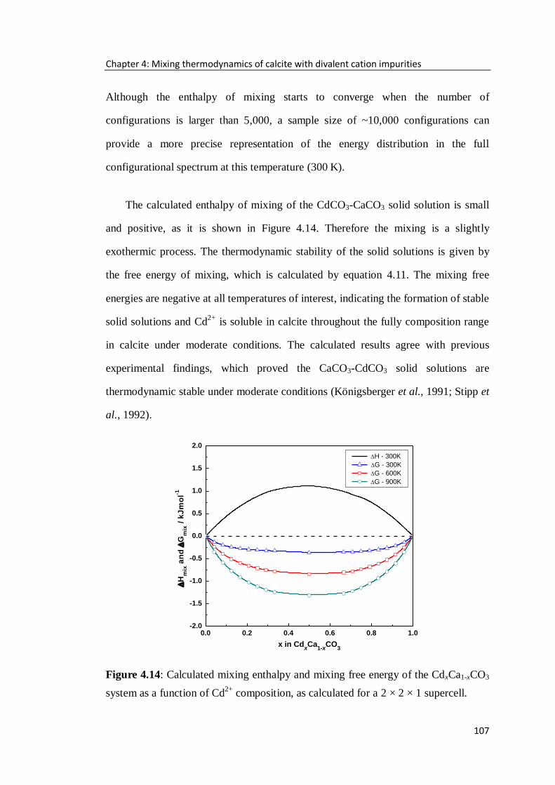
Chapter 4: Mixing thermodynamics of calcite with divalent cation impurities
107
Although the enthalpy of mixing starts to converge when the number of
configurations is larger than 5,000, a sample size of ~10,000 configurations can
provide a more precise representation of the energy distribution in the full
configurational spectrum at this temperature (300 K).
The calculated enthalpy of mixing of the CdCO3-CaCO3 solid solution is small
and positive, as it is shown in Figure 4.14. Therefore the mixing is a slightly
exothermic process. The thermodynamic stability of the solid solutions is given by
the free energy of mixing, which is calculated by equation 4.11. The mixing free
energies are negative at all temperatures of interest, indicating the formation of stable
solid solutions and Cd2+
is soluble in calcite throughout the fully composition range
in calcite under moderate conditions. The calculated results agree with previous
experimental findings, which proved the CaCO3-CdCO3 solid solutions are
thermodynamic stable under moderate conditions (Königsberger et al., 1991; Stipp et
al., 1992).
0.0 0.2 0.4 0.6 0.8 1.0-2.0
-1.5
-1.0
-0.5
0.0
0.5
1.0
1.5
2.0
H - 300K
G - 300K
G - 600K
G - 900K
H
mixa
nd
G
mix
/ k
Jm
ol-1
x in CdxCa
1-xCO
3
Figure 4.14: Calculated mixing enthalpy and mixing free energy of the CdxCa1-xCO3
system as a function of Cd2+
composition, as calculated for a 2 × 2 × 1 supercell.

Chapter 4: Mixing thermodynamics of calcite with divalent cation impurities
108
Besides the free energy of mixing ΔGmix, it is common to report the excess free
energy GE of the solid solution, defined as:
E ideal
mix mixG G G (4.14)
ideal
mixG is the free energy of mixing in an ideal solid solution, where the only
contribution comes from the ideal entropy corresponding to a fully disordered solid.
[ ln (1 )ln(1 )]ideal
mix BG k T x x x x (4.15)
The excess free energy GE therefore contains all the non-ideal contributions to the
mixing free energy: an enthalpy part (ΔHmix) and an entropy part, which contains
both the deviation of the configurational entropy from ideality and a contribution
from the vibrational entropy of mixing.
0.0 0.2 0.4 0.6 0.8 1.0-13
-11
-9
-7
-5
-3
-1
1
3
Theory - this work
Theory - Lippmann (1980)
Theory - Mandell et al. (1999)
Experiment - Rock et al. (1994)
x in CdxCa
1-xCO
3
GE /
kJ
mo
l-1
Figure: 4.15: Comparison between theoretical and experimental excess free energies
GE findings for CdxCa1-xCO3 at 300 K.
Figure 4.15 shows a comparison of the calculated excess free energy GE for
CdxCa1-xCO3 at 300 K with the theoretical GE prediction of Lippmann‟s electrostatic

Chapter 4: Mixing thermodynamics of calcite with divalent cation impurities
109
model (1980), Mandell et al.‟s (1999) lattice energy model and Rock et al.‟s (1994)
experimental findings, which are based on electrochemical cell-voltage measurement.
The positive excess free energy indicates the mixing in CdCO3-CaCO3 solid solution
is non-ideal. The calculated theoretical values are not far from the GE results by
Lippmann (1980). The experimental results by Rock et al., on the other hand,
contrast significantly with the theoretical results. The difference of excess free
energy between theoretical calculation and experimental measurement is expected
because the magnitude of the estimated GE is sensitive to the choice of free energy of
formation of CdCO3, which is uncertain in the experiments.
4.6 FeCO3-CaCO3 solid solutions
Siderite (FeCO3) is commonly found in hydrothermal veins and at shallow burial
depths in sedimentary rocks. It also has the calcite-type structure, but as the ionic
radius of Fe2+
(0.75Å) is only three quarters of that of Ca2+
in six-fold coordination,
there should be obvious effect on the local structure of calcite. The variation of the
configurational entropy of the (Fe,Ca)CO3 system with temperature also indicates
that some degree of cation ordering should be expected in the FeCO3-CaCO3 solid
solutions (see Figure 4.4).
The intermediate composition Fe0.5Ca0.5CO3 has never been detected in the
natural environment. The enthalpy of mixing ΔHmix was calculated in successive
groups from 1000 to 10,000 configurations by the random sampling method. The
lowest energy arrangement of cations corresponds to the dolomite-type structure, and
its lattice energy is 110 kJmol-1
(4.6 kJmol-1
per formula unit) lower than the least
stable configuration found in the random sampling. Although the number of
configurations with more homogeneous Fe2+
distributions is larger than the ordered
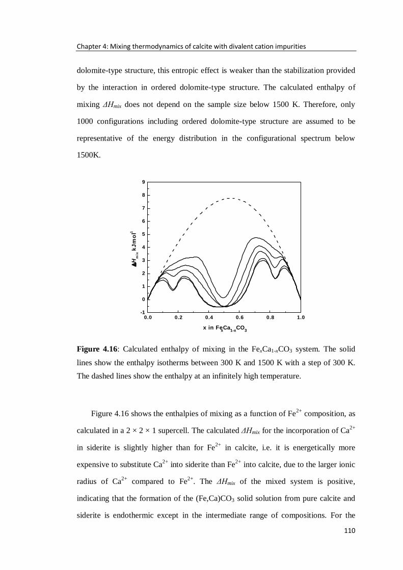
Chapter 4: Mixing thermodynamics of calcite with divalent cation impurities
110
dolomite-type structure, this entropic effect is weaker than the stabilization provided
by the interaction in ordered dolomite-type structure. The calculated enthalpy of
mixing ΔHmix does not depend on the sample size below 1500 K. Therefore, only
1000 configurations including ordered dolomite-type structure are assumed to be
representative of the energy distribution in the configurational spectrum below
1500K.
0.0 0.2 0.4 0.6 0.8 1.0-1
0
1
2
3
4
5
6
7
8
9
x in FexCa
1-xCO
3
H
mix k
Jm
ol-1
Figure 4.16: Calculated enthalpy of mixing in the FexCa1-xCO3 system. The solid
lines show the enthalpy isotherms between 300 K and 1500 K with a step of 300 K.
The dashed lines show the enthalpy at an infinitely high temperature.
Figure 4.16 shows the enthalpies of mixing as a function of Fe2+
composition, as
calculated in a 2 × 2 × 1 supercell. The calculated ΔHmix for the incorporation of Ca2+
in siderite is slightly higher than for Fe2+
in calcite, i.e. it is energetically more
expensive to substitute Ca2+
into siderite than Fe2+
into calcite, due to the larger ionic
radius of Ca2+
compared to Fe2+
. The ΔHmix of the mixed system is positive,
indicating that the formation of the (Fe,Ca)CO3 solid solution from pure calcite and
siderite is endothermic except in the intermediate range of compositions. For the

Chapter 4: Mixing thermodynamics of calcite with divalent cation impurities
111
intermediate compositions, the ΔHmix curves overlap each other below 1200 K as a
result of higher weighting of the lower-energy configuration (dolomite-type
structure). These results do not completely coincide with the native enthalpy of
mixing of the mixed systems at low temperatures, as other mixed layered ordering
structure like the dolomite-type structure, may also be present in the whole
configurational spectrum.
0.0 0.2 0.4 0.6 0.8 1.0-2
-1
0
1
2
3
300 K
600 K
1000 K
1400 K
G
mix
/ k
J m
ol-1
x in FexCa
1-xCO
3
Figure 4.17: Calculated free energy of mixing of the FexCa1-xCO3 system as a
function of Fe2+
compositions.
The thermodynamic stability of (Fe,Ca)CO3 solid solution is given by the free
energy of mixing calculated by equation 4.11 between 300 K and 1400 K, as
illustrated in Figure 4.17. The maximum solubility of Fe in calcite is very close to x
= 0.4 at 1000 K. The free energy of mixing is negative for full Fe compositions
above1400 K, and there are two minima at xc = 0.33 and xs = 0.96, which define a
miscibility gap between calcite and siderite. The solid with composition between xc <
x < xs is thermodynamically metastable with respect to a mechanical mixture of
xc xs

Chapter 4: Mixing thermodynamics of calcite with divalent cation impurities
112
phases with composition xc and xs. The prediction of a miscibility range in the
FexCa1-xCO3 solid solutions is in agreement with experimental studies. Goldsmith
(1959) reported that the lower limit of the miscibility gap is 0.37 at 973 K, whereas
Rosenberg (1963) predicted the miscibility gap between 0.17 < x < 0.85 at 823 K. It
is noteworthy that the intermediate compositions are metastable and could not
precipitate below 1400 K, which also confirmed the experimental findings. The
dolomite-type Fe0.5Ca0.5CO3 has never been reported as a natural mineral and it is not
a stable phase in the temperature range from 573 K to 823 K.
0.00 0.05 0.10 0.15 0.20-1
0
1
2
3
4
5
Theory - This work
Theory - Davies and Navrotsky (1983)
Theory - Lippmann (1980)
Theory - Mandell et al. (1999)
x in FexCa
1-xCO
3
GE /
kJ
mo
l-1
Figure 4.18: Comparison between theoretical excess Gibbs free energies GE for the
FexCa1-xCO3 solid solutions at 823 K.
The results of excess free energy GE for the FexCa1-xCO3 system are displayed in
Figure 4.18, together with theoretical finding by other authors. The positive excess
free energy indicates the mixing in the FexCa1-xCO3 solid solution is non-ideal.
Davies and Navrotsky (1983) obtained positive GE for the FexCa1-xCO3 system from
573 K to 1073 K using a sub-regular solution model containing empirically

Chapter 4: Mixing thermodynamics of calcite with divalent cation impurities
113
thermodynamic interaction parameters. Mandell et al. (1999) used an extending
lattice energy calculation model to investigate the pure carbonate minerals and also
predicted positive excess free energy at 823 K. The theoretical excess energies
addressed in this work are consistent with these theoretical results by other authors.
4.7 Uptake of Zn2+
and Co2+
to calcite
The ionic radii and coordination distances to oxygen of Zn2+
and Co2+
in six-fold
coordination are very similar. Smithsonite (ZnCO3) is commonly found in the natural
environment, whereas cobalt calcite (CoCO3) is rare in nature. Smithsonite can form
limited solid solutions with rhodochrosite and siderite. However, substitution of Co2+
in the structure of the common rhombohedral carbonates is not observed to any
significant extent in nature, unlike the commonly observed substitutions of Zn2+
.
Various studies have used kinetic-spectroscopic techniques to investigate the
interaction of Zn2+
with calcite. All experimental findings have shown a strong
adsorbing behaviour of Zn2+
on the calcite surface, which can be described best by a
Langmuir model (Zachara et al., 1988; Temmam et al., 2000; El-Korashy, 2003). For
example, a spectroscopy study of synthetic and natural calcite samples containing
traces of Zn2+
by Reeder et al. (1999) confirmed the substitution of Zn2+
for Ca2+
in
octahedral coordination occurs via exchange with Ca2+
in a surface-adsorbed layer.
The presence of large amounts of Zn2+
in a Ca2+
/CO32-
-bearing fluid reduces the
growth rate of calcite, hinders the crystallisation of calcite and favours the formation
of hydrozincite or aragonite (Glasner et al., 1980; Meyer, 1984; Wada et al., 1995).
Freij et al. (2004) used AFM and batch sorption experiments to study the interaction
of Zn2+
with calcite {1 0 4} surfaces during growth and dissolution. Their results
showed that the growth of calcite in the presence of Zn2+
occurs by two-dimensional

Chapter 4: Mixing thermodynamics of calcite with divalent cation impurities
114
nucleation, the growth rate decreasing with the development of each subsequent layer.
All these studies provided significant information on the strong interaction of Zn2+
with calcite under different conditions, using various techniques. However, none
dealt with the thermodynamic properties of the (Zn,Ca)CO3 solid solutions at the
atomic level, which are needed to understand the mechanism of adsorption and
substitution.
At first the mixing enthalpies ΔHmix of intermediate composition Zn0.5Ca0.5CO3
and Co0.5Ca0.5CO3 in a 2 × 2 × 1 supercell have been calculated, based on the random
sampling method. Because of the strong stabilization provided by the interaction in
the ordered dolomite-type structure, the mixing enthalpies ΔHmix of both systems do
not change with increasing sample size below 1500 K, which are similar to that of
the (Fe,Ca)CO3 system. Again, only the ordered dolomite-type configuration has
been used in the calculation of the mixing free energy rather than the average of the
whole configuration spectrum of Zn0.5Ca0.5CO3 and Co0.5Ca0.5CO3 below 1500 K.
Figure 4.19: Calculated free energy of mixing with full range of Co2+
or Zn2+
compositions; (a) CoxCa1-xCO3, (b) ZnxCa1-xCO3.
0.0 0.2 0.4 0.6 0.8 1.0-2
-1
0
1
2
3
4
300 K
1000 K
1500 K
G
mix
/ k
J m
ol-1
x in CoxCa
1-xCO
3
0.0 0.2 0.4 0.6 0.8 1.0-2
-1
0
1
2
3
4
5
300 K
1000 K
1500 K
G
mix
/ k
J m
ol-1
x in ZnxCa
1-xCO
3
(a) (b)
xc xc
Chapter 4: Mixing thermodynamics of calcite with divalent cation impurities
115
The mixing free energy of the ZnxCa1-xCO3 and CoxCa1-xCO3 systems are
calculated by equation 4.11 between 300 K and 1500 K, respectively. For the
CoxCa1-xCO3 system (see Figure 4.19a), CoCO3 is soluble in calcite below the Co2+
composition x = 0.06 at 1000 K, and the solubility is close to x = 0.34 at 1500 K. The
solubility of ZnCO3 in calcite (see Figure 4.19b) is x < 0.04 at 1000 K and x < 0.35 at
1500 K, which is similar to that of CoCO3. The free energy of mixing ΔGmix for Co2+
or Zn2+
is positive for the compositions x > 0.6 indicating Ca2+
can be soluble in
neither CoCO3 nor ZnCO3 below 1500 K.
The calculated miscibility range is not far from the experimental findings.
Goldsmith and Northrop (1965) reported that the limit of the miscibility of
CoxCa1-xCO3 is x = 0.04 at 873 K and x = 0.15 at 1073 K. Limited coprecipitation of
Zn2+
with CaCO3 has also been observed between 300 K and 523 K (Crocket and
Winchester, 1966; Tsusue and Holland, 1966). Furthermore, although the free
energies of mixing of the intermediate composition Co0.5Ca0.5CO3 and Zn0.5Ca0.5CO3
are negative, these mixed systems are metastable and tend to change into a Ca-rich
phase below 1500 K, which also confirms that the dolomite-type Co0.5Ca0.5CO3 or
Zn0.5Ca0.5CO3 does not exist in synthesis or nature (Goldsmith and Northrop, 1965).
4.8 Uptake of Mg2+
and Ni2+
to calcite
The ionic radii of Mg2+
(0.65 Å) and Ni2+
(0.72 Å) are much smaller than Ca2+
(1.00 Å). Former studies indicate that it is energetically favourable for Mg2+
to
substitute Ca2+
in calcite due to the smaller ionic radius (Fork, 1974; Davis et al.,
2000). Magnesite (MgCO3) and dolomite (MgCa(CO3)2) typically occur in nature,
but nickel carbonate (NiCO3) has never been known as a mineral. Comparing with
one of the best studied carbonate system (Mg,Ca)CO3, the (Ni,Ca)CO3 system is still

Chapter 4: Mixing thermodynamics of calcite with divalent cation impurities
116
less researched by experiment due to the decomposition of carbonates.
The (Mg,Ca)CO3 system is one of the best studied metal calcite systems.
Magnesium is considered as an important modifier of CaCO3 growth and
morphologies in aqueous solution. Although the presence of Mg2+
in CaCO3 is
studied increasingly, the physical basis by which Mg2+
modifies calcite growth has
yet to be discerned. Bulk studies have suggested that the growth of calcite is
inhibited through either step-blocking by Mg2+
adsorption and slow dehydration
(Lippman, 1960; Gutjahr et al., 1996) or enhanced mineral solubility associated with
lattice strain caused by the incorporated Mg2+
(Fork, 1974; Berner, 1975). Davis et al.
(2000) used AFM to resolve the mechanism of calcite inhibition by Mg2+
at the
molecular scale and determine the thermodynamic and kinetic controls of Mg2+
on
calcite formation. Their experiments demonstrated that Mg2+
inhibits calcite growth
by incorporation into the calcite lattice. The resultant increase in the mineral
solubility forms the underlying physical basis for the reduced calcite growth rates
observed in the presence of Mg2+
. Hence a further understanding of the (Mg,Ca)CO3
solid solution requires an accurate assessment as to how Mg2+
modifies the calcite
growth via solubility.
The structure and cationic ordering behaviour for the intermediate composition
of dolomite (Mg0.5Ca0.5CO3) and Ni0.5Ca0.5CO3 were initially investigated at different
temperatures based on the random sampling method. The lowest energy arrangement
of cations in the whole configurational spectrum corresponds to the dolomite-type
structure. The least stable configuration found in the random sampling had a lattice
energy of 148.5 kJmol-1
(6.2 kJmol-1
per formula unit) higher than the ordered
dolomite structure. The lattice energy of dolomite-type Ni0.5Ca0.5CO3 is 279.5
kJmol-1
(11.6 kJmol-1
per formula unit) lower than that of the least stable
configuration. The stabilization provided by the interaction within the ordered
Chapter 4: Mixing thermodynamics of calcite with divalent cation impurities
117
dolomite structure is so strong that there will be no configurational entropy
contributions to the free energy of mixing ΔGmix of the intermediate compositions
below 1500 K. Therefore, the lattice energy of the dolomite-type configuration can
be assumed to be equal to the average enthalpy of intermediate compositions
Mg0.5Ca0.5CO3 and Ni0.5Ca0.5CO3 below 1500 K.
The solubility of Mg2+
in calcite was then evaluated by calculating the free
energy of mixing ΔGmix between calcite and ordered dolomite phase (equation 4.16, 0
< x <0.5), or between dolomite and magnetite (equation 4.17, 0.5 < x < 1) as a
function of Mg2+
compositions at a range of temperatures:
1
1 3 3 0.5 0.5 3[ ] (1 2 ) [ ] 2 [ ]mix x xG G Mg Ca CO x U CaCO xU Mg Ca CO
(4.16)
2
1 3 3 0.5 0.5 3[ ] (2 1) [ ] (2 2 ) [ ]mix x xG G Mg Ca CO x U MgCO x U Mg Ca CO
(4.17)
where G[MgxCa1-xCO3] is the free energy of the mixed system, and U[Mg0.5Ca0.5CO3]
is the lattice energy of the pure dolomite, as there is no configurational entropy
contributions to the free energy of the stable dolomite.
Figure 4.20 displays the calculated free energy of mixing ΔGmix in the binary
systems of calcite-dolomite and dolomite-magnetite from 500 K to 1500 K. The
solubility of Mg2+
in calcite is up to x = 0.04 at 1000 K. The ΔGmix is negative for the
Mg2+
composition 0 < x < 0.33 at 1500 K, which suggests magnesian calcite and
dolomite can form stable solid solutions at this temperature, where the Mg2+
compositions in the stable phase is at least up to 0.33. This miscibility between
magnesian calcite and dolomite agrees with the experiments by Goldsmith and Heard
(1961), where the top of the solvus outlining the two-phase field is at Mg2+
composition x = 0.43 at 1348 K, and above the solvus a single-phase region extends
from calcite to dolomite. Conversely, the miscibility gap between dolomite and

Chapter 4: Mixing thermodynamics of calcite with divalent cation impurities
118
magnesite is considerably wider and the solubility of Ca2+
in magnesite is up to 0.04
at 1500 K.
Figure 4.20: Calculated free energy of mixing of the binary (Mg,Ca)CO3 system as a
function of Mg2+
composition, (a) calcite-dolomite, (b) dolomite-magnetite.
Subsequently, the solid solubility in (Ni,Ca)CO3 solid solutions has been
evaluated by calculating the free energy of mixing ΔGmix between calcite, ordered
dolomite-type Ni0.5Ca0.5CO3 and NiCO3. The dolomite-type Ni0.5Ca0.5CO3 was
assumed to be a stable phase below 1500 K in this calculation, although it does not
exist in nature. The calculated free energy of mixing ΔGmix in the binary systems of
CaCO3 - Ni0.5Ca0.5CO3 and Ni0.5Ca0.5CO3 - NiCO3 from 500 K to 1500 K are showed
in Figure 4.21. A simple inspection of the results shows that in both cases the free
energies of mixing are positive from 500 K to 1500 K. As such there can be neither
Ni2+
substitution in calcite nor Ca2+
substitution in NiCO3 even at high temperatures
(e.g. ~1500 K). Furthermore, the dolomite-type structure Ni0.5Ca0.5CO3 is not stable
due to the limit substitution of Ni2+
in calcite and vice versa.
0.6 0.7 0.8 0.9 1.0-0.5
0.0
0.5
1.0
1.5
2.0
1000 K
1500 K
G
mix
/ k
J m
ol-1
x in MgxCa
1-xCO
3
0.0 0.1 0.2 0.3 0.4-2.0
-1.5
-1.0
-0.5
0.0
0.5
1.0
1.5
2.0
500 K
1000 K
1500 K
G
mix
/ k
J m
ol-1
x in MgxCa
1-xCO
3
(a) (b)
xc xs

Chapter 4: Mixing thermodynamics of calcite with divalent cation impurities
119
Figure 4.21: Calculated free energy of mixing of the binary systems as a function of
Ni2+
composition. (a) CaCO3-Ca0.5Ni0.5CO3, (b) Ca0.5Ni0.5CO3-NiCO3
4.9 Chapter summary
The mixing thermodynamics of binary CaCO3-MeCO3 solid solutions (Me = Mg,
Ni, Co, Zn, Fe, Mn and Cd) in the whole range of Me2+
compositions have been
investigated by atomistic simulation techniques. The ionic radius, coordination
distance and solubility of divalent cations in calcite are summarised in Table 4.2.
The calculations show that CdCO3 and CaCO3 form a continuous stable solid
solution in the whole Cd2+
compositions at moderate temperatures. While there is a
miscibility gap at Mn2+
composition 0.12 < x < 0.92 in the (Mn,Ca)CO3 system,
which contains a small degree of cationic ordering rather than the expected
completely random distribution. A higher abundance of cation ordering is present in
the (Fe,Ca)CO3, (Co,Ca)CO3, (Zn,Ca,)CO3, (Mg,Ca)CO3 and (Ni,Ca)CO3 systems,
and the solubility of these cations in calcite is thus very limited. All investigated
carbonate systems show higher solubility of the smaller ions in calcite than that of
Ca2+
in the other end-member carbonates. The dolomite-type compounds
0.0 0.1 0.2 0.3 0.4-1
0
1
2
3
4
5
500 K
1000 K
1500 K
G
mix
/ k
J m
ol-1
x in NixCa
1-xCO
3
0.6 0.7 0.8 0.9 1.0-2
0
2
4
6
8
10
500 K
1000 K
1500 K
G
mix
/ k
J m
ol-1
x in NixCa
1-xCO
3
(a) (b)

Chapter 4: Mixing thermodynamics of calcite with divalent cation impurities
120
Me0.5Ca0.5CO3, are not observed to form with Cd2+
, Fe2+
, Co2+
, Zn2+
and Ni2+
. For
Mn2+
, the ordered kutnahorite is metastable and behaves disorder above 695 K.
According to the calculations, the solubility of impurity cations in calcite, which is in
good agreement with available experimental results, is largely related to the cationic
coordination distance with oxygen. Ionic radius is clearly not the controlling factor in
these binary carbonate solid solutions.
Table 4.2 Some data on rhombohedral carbonates.
Cations Radius
/ Å
Me-O
/ Å
Solubility in
calcite
(calculation)
Solubility in
calcite
(experiment)
Dolomite
type
structure
Ca2+
1.00 2.40 complete (300 K) complete (298 K) /
Cd2+
0.97 2.26 complete (300 K) complete (298 K) No
Mn2+
0.83 2.16 x < 0.12 (900 K) x < 0.13 (298 K) Yes
Fe2+
0.75 2.12 x < 0.4 (1000 K) x < 0.35 (1023 K) No
Co2+
0.72 2.10 x < 0.06 (1000 K) x < 0.13 (1023 K) No
Zn2+
0.75 2.09 x < 0.04 (1000 K) x < 0.2 (1023 K) No
Mg2+
0.65 2.08 x < 0.04 (1000 K) x < 0.12 (1023 K) Yes
Ni2+
0.72 1.99 no x < 0.05 (1023 K) No

121
5 Investigation of the interaction between
calcite nanoparticle and calcite surfaces
When two calcite particles collide in the solution, the interaction between the
particles holds them together for a short while before they are separated by the fluid
shear force. If the interaction is strong, or the particles are growing quickly, the
particles will remain bound together to form an aggregate. In this chapter atomic
simulation techniques have been applied to establish the key factors that affect the
interaction between a calcite nanoparticle and some major calcite surfaces. Both
planar and stepped surfaces in vacuum and aqueous environment have been
considered. This study provides quantitative information for experimental studies of
the aggregation of calcite nanoparticles during the crystal growth process.

Chapter 5: Investigation of the interaction between calcite nanoparticle and calcite surfaces
122
5.1 Introduction
Recently, the growth of calcite has been studied extensively both in experiments
(Dobson et al. 2005; Wasylenki et al. 2005) and computational modelling (de Leeuw
et al. 1999; de Leeuw 2002), and calcite particles on the micro-scale (i.e.
nanoparticles) have gained increasing attention due to their fundamental role in
calcite crystal growth, where the aggregation of nanoparticles can lead to the
formation of crystals with different morphologies (Colfen, 2003; Domingo, 2004).
Aggregation of calcite particles could arise from a combination of many effects:
solid-state properties, growth habit and crystallization conditions, such as solution
supersaturation and flow rate. However, it is still not fully understood how we can
achieve control over this process.
The aggregation between a small nanoparticle and a larger nanoparticle can be
approximated as the adhesion of a small nanoparticle onto a substrate, namely a large
surface. In this chapter the epitaxial matching of calcite nanoparticles to a number of
common calcite surfaces has been investigated by using computer modelling at the
atomic level. By separately modelling calcite nanoparticle with different morphology
and substrate, it is possible to comment on the effect of lattice matching on the
adhesion energy and explain experimental findings during the calcite crystal
aggregation process.
5.2 Calcite surfaces
The rhombohedral structure of calcite, which has a space group R c, hexagonal
lattice vectors a = b = 4.990 Å, c = 17.061 Å (Deer et al., 1992), was used as the
starting bulk structure. The computer code METADISE (Watson et al., 1996) was

Chapter 5: Investigation of the interaction between calcite nanoparticle and calcite surfaces
123
then employed to optimise the bulk structure and resulting structure was used to
create the planar and stepped surfaces. Two planar surfaces {1 0 4}, {0001} and
two stepped surfaces {3 1 8}, {3 16} are considered in this study. A series
of simulations were carried out to determine the optimised structures and surface
energies of the cleaved surfaces in vacuum. The results are listed in Table 5.1.
Table 5.1 Surface energies of pure calcite surfaces (Jm-2
)
surface unrelaxed surface relaxed surface
{1 0 4} 0.64 0.57
{0001}-CO32-
1.59 0.98
{0001}-Ca2+
2.39 0.99
{3 1 8} 1.15 0.88
{3 16} 0.91 0.72
The {1 0 4} surface is the most stable surface of calcite and dominates its
observed morphology. It consists of layers of calcium, carbon and one oxygen atom
in a plane with the other two oxygen atoms above and below this plane, as shown in
Figure 5.1a. It has a higher density of ions compared with other possible charge
neutral planes, leading to its low surface energy and stability. The {0001} surface is a
common twinning plane, which according to Pastero‟s statistical work (2004) occurs
to almost 17% in natural calcite samples. The {0001} surface contains alternating
planes of Ca2+
and CO32-
groups, which produces a dipole moment perpendicular to
the surface. Polar surfaces are unstable by themselves and will either reconstruct to
neutralize the dipole moment or adsorb ions to remove the dipole moment. In this
study, the dipole moment is removed by moving half the ions from the top layer of
the surface to the bottom, creating surface vacancies in the process. As a result two
{0001} surfaces with different terminations have been created, namely a CO32-

Chapter 5: Investigation of the interaction between calcite nanoparticle and calcite surfaces
124
terminated surface (Figure 5.1b) and a Ca2+
terminated surface (Figure 5.1c).
(a)
(a)
(b)
(c)
Figure 5.1: Top view and side views of pure planar surfaces, (a) {10 4} surface, (b)
CO32-
terminated {0001} surface and (c) Ca2+
terminated {0001} surface. The second
plane in the top view has been omitted for clarity. (Ca = green, C = grey, O = red).
Stepped surfaces are usually present in natural and synthesized calcite crystals
and experimental systems. Steps on the calcite cleavage face are common along the
crystallographic directions defined by cleavage plane intersections. Because calcite
has a rhombohedral lattice, two non-equivalent steps are produced by each of the
cleavage planes that intersect at the surface. These steps differ in their local atomic
arrangement and are named the acute and obtuse step by the angle they make with
Y
X
Y
X
Y
X
[1014]
[0001]
[0001]
Z
X
Z
X
Z
X

Chapter 5: Investigation of the interaction between calcite nanoparticle and calcite surfaces
125
the surface (Kristensen and Stipp, 2004). There are many surfaces that include these
steps, but the surfaces on which the steps are closest together are the {3 1 8} and
{3 16} surfaces, as illustrated in Figure 5.2, describing a plane with acute and
obtuse steps, respectively. On the acute stepped {3 1 8} surface, the CO32-
groups
on the edge overhang the plane below, forming an angle of 80o with the lower plane.
On the obtuse stepped {3 16} surface, the CO32-
groups on the step edge lean
backwards with respect to the below plane, forming an angle of 105o with the lower
plane. Both {3 1 8} and {3 16} surfaces contain {1 0 4} terraces and
monatomic steps. The side walls of the steps are also {1 0 4} planes and the step
edges of the two stepped surfaces are identical to the two different edges of the
calcite rhomb.
Figure 5.2: Side view of pure stepped surfaces, (a) acute {3 1 8} surface and (b)
obtuse {3 16} surface. (Ca = green, C = grey, O = red).
As calcite is usually present in an aqueous environment, it is essential to include
water in the simulations. Many experiments and computer simulations have indicated
that water molecules organize into ordered layers in the mineral-water interface. For
example, a classic molecular dynamics study by Kerist and Parker (2004) has found
that there are three ordered layers of water on the calcite {1 0 4} surface. The
existence of this arrangement is supported by experimental X-ray scattering data
(Geissbühler et al., 2004), which found two water layers on the calcite surface in
(b) 105o
Z
Y
Z
X
(a) 80o

Chapter 5: Investigation of the interaction between calcite nanoparticle and calcite surfaces
126
bulk water. This is expected to be a general effect at ionic surfaces. Previous studies
of water adsorption at surfaces have shown that there is a clear difference between
the water adsorbed at the mineral surface and bulk water, and only the adsorbed
layering water molecules were shown to affect the structure and energy of the
underlying surface. For these reasons, both monolayer and multi-layer water on the
calcite surfaces were considered in this study.
At first, only a full monolayer of water molecules was added to the surface,
which is defined as the maximum number of water molecules adsorbed at the surface
in a single layer without formation of a second layer. Ca2+
sites at the top plane were
selected as initial positions for adding the water molecules and the oxygen atoms in
water molecules were placed at a distance of 2.0 Å above the Ca2+
sites. Surface
calculations were carried out to determine the surface energies of the hydrated
surfaces, which are listed in Table 5.2. It is clear that the surface energies of the
hydrated surfaces are smaller than those of corresponding pure surfaces. It is evident
that the adsorbed water molecules have a stabilizing effect on the surfaces.
Table 5.2 Surface energies of hydrated calcite surfaces (Jm-2
)
surface surface energy
{1 0 4} 0.16
{0001}-CO32-
0.42
{0001}-Ca2+
0.63
{3 1 8} 0.78
{3 16} 0.60
Figure 5.3 shows a top view of the structures of the hydrated planar surfaces,
where a very regular pattern of adsorbed water molecules presents on the planar

Chapter 5: Investigation of the interaction between calcite nanoparticle and calcite surfaces
127
surfaces. The adsorbed water molecules lie flat on the {1 0 4} surface, which
agrees with experimental and other computational findings on adsorption of water on
calcite surfaces (Chang et al., 1995; de Leeuw and Parker, 1997). Adsorption of
water on the {0001} surface is more complicated. The water molecules show a clear
tendency to cluster around the surface CO32-
groups (Figure 5.3b) or the surface Ca2+
atoms (Figure 5.3c) relaxing into the vacancies created by shifting half the CO32-
groups or Ca2+
ions to the bottom of the surface as described in the chapter 2.
(a)
(b)
(c)
Figure 5.3: Top view and side view of hydrated planar surfaces with monolayer of
water, (a) {1 0 4} surface, (b) CO32-
terminated {0001} surface and (c) Ca2+
terminated {0001} surface. (Ca = green, C = grey, O = red, H = white, Owater = blue).
Y
X
Y
X
Y
X
[1014]
[0001]
[0001]
Z
X
Z
X
Z
X

Chapter 5: Investigation of the interaction between calcite nanoparticle and calcite surfaces
128
In the cases of stepped surfaces, the presence of a step does not greatly affect the
regular arrangement of water molecules that was in direct contact with the terraces.
However, the arrangement of water molecules right next to the step was disrupted. At
the acute step, the water molecules initially coordinated with Ca2+
at the step edge
delocalize the possible adsorption sites, implying the water molecules are less
strongly bound to the stepped surface than a planar surface. On the contrary, as Ca2+
at the step edge of the obtuse step creates new adsorption sites, the water molecules
are much strongly bound to the obtuse step than the acute step (Figure 5.4).
Figure 5.4: Side view of hydrated stepped surfaces with monolayer of water, (a)
acute {3 1 8} surface and (b) obtuse {3 16} surface (Ca = green, C = grey, O
= red, H = white, Owater = blue)
More layers of water were then introduced in a similar manner and each time an
extra layer of water (24 molecules) was placed at a distance of 2.0 Å above the top of
existing hydrated surfaces. In total, four layers of water (96 molecules) were added
onto each surface, which build about 8 Å water layers above the pure surface. The
calcite-water interfacial systems were then equilibrated by molecular dynamics
simulations, using the DL_POLY 2.20 code (Smith and Forester, 1996), where a
combination of NVE and NVT ensembles were used in sequence at a temperature of
300 K. The Nosé-Hoover thermostat was set at 0.1 ps and the relaxation time of
barostat was set at 0.5 ps in the calculations. The trajectories were generated using
(a) (b)
Z
X
Z
Y
Chapter 5: Investigation of the interaction between calcite nanoparticle and calcite surfaces
129
the Verlet Leap-Frog algorithm using a time step of 0.2 fs. The simulation cell was
equilibrated for 100 ps, after which data were collected for another 200 ps. The final
hydrated structure was then used as the substrate for the adhesion of the calcite
nanoparticle.
5.3 CaCO3 nanoparticle
The CaCO3 nanoparticle is constructed from the optimised bulk structure of
calcite using the METADISE code as described in the methodology chapter. The
morphology of the calcite particle is determined by the intersection of the cleavage
planes, and surfaces with low surface energy lie on the outside of the polyhedron.
The volume enclosed by this polyhedron is then filled with atoms based on periodic
repeats of the lattice motif, thus generating an initial structure for a nanoparticle.
Due to the low surface energy (0.57 Jm-2
) of the {1 0 4} surface, the most
stable calcite nanoparticle should consist of {1 0 4} surfaces. However, some
experimental studies (Rajam and Mann, 1990; Pastero et al. 2004) have suggested
that the morphology of calcite does not only consist of {1 0 4} surfaces, but also
contains the {0001} surface, when Li+ is present in the aqueous solution. Therefore,
three CaCO3 nanoparticles with different morphologies were considered in this study,
by using the surface energy of the {1 0 4}, {0001}-Ca2+
and {0001}-CO32-
,
respectively, as shown in Figure 5.5. In this thesis, nanoparticle104, nanoparticle001-Ca
and nanoparticle001-CO3 are used to label three CaCO3 nanoparticles, consisting of
{10 4} surface, {0001}-Ca2+
surface and {0001}-CO32-
surface, respectively. The
nanoparticle104 is constructed as a 1.0 nm rhombohedra with {1 0 4} surfaces on
the outside, which contains 18 CaCO3 units. The nanoparticle001 is constructed as a
multi-prism with {0001} surface on both top and bottom of the prism, where both

Chapter 5: Investigation of the interaction between calcite nanoparticle and calcite surfaces
130
Ca2+
and CO32-
terminated {0001} surfaces are considered. The 1.0 nm
nanoparticle001-Ca contains 38 CaCO3 units, while the 1.2 nm nanoparticle001-CO3
contains 61 CaCO3 units.
(a) (b) (c)
Figure 5.5: Morphology of CaCO3 nanoparticle, showing (a) {1 0 4} surface (b)
{0001}-Ca2+
surface and (c) {0001}-CO32-
surface.
5.4 Adhesion energy of a nanoparticle on the surface
A nanoparticle-surface interfacial system consists of a calcite nanoparticle and a
pure or hydrated calcite surface. To ensure a large number of interfacial
configurations are sampled in the study, a comprehensive range of positions of the
nanoparticle with respect to the calcite surface was examined, including a series of
heights and orientations as well as lateral displacement of the nanoparticle. The
vertical distance of the nanoparticle with respect to the surface has been investigated
from 1 Å to 10 Å, and for each height, different orientations of the nanoparticle have
been considered, where the angle of the rotation θ (θ is the rotation angle in x/y
axles), was varied by 30o in turn. The initial orientation of the nanoparticle of θ = 0
o
is assumed, where the lattices of the nanoparticle and the pure surface are perfectly
aligned. Figure 5.6 shows a calcite nanoparticle104 with a rotation of θ = 0o and θ =
60o with respect to the {1 0 4} surface.
{10 4}
{0001}-Ca2+
{0001}-CO32-

Chapter 5: Investigation of the interaction between calcite nanoparticle and calcite surfaces
131
(a) θ = 0o (b) θ = 60
o
Figure 5.6: Examples of a calcite nanoparticle104 on the top plane of planar {1 0 4}
surface. (Ca = green, C = grey, O = red).
Prior to energy minimisation of the interfacial systems, the calcite nanoparticle is
kept at a constant height above the surface, but moved systematically in two
directions over the surfaces without relaxation of the surface or the nanoparticle. The
interfacial energy for the unrelaxed system is calculated for a series of points on a
grid. The grid was determined by the surface lattice vectors of the systems in two
directions at intervals of 0.5 Å. This scan supplies the information of interfacial
energy at each point on the grid, hence identifying the lowest energy lateral
displacement of the nanoparticle with respect to the surface in the unrelaxed system.
The configuration with the lowest energy is then used as the starting point and a full
geometry optimisation is performed to obtain the energy for the relaxed system.
Newton-Raphson optimisation algorithm is used for the full geometry optimisation.
During the geometry optimisation, both the nanoparticle and surfaces are completely
unconstrained.
The adhesion energy per CaCO3 group in the bottom plane of the nanoparticle
was calculated using the equation below:
int
1[ ( )]adhesion erfacial surface particleU U U U
n (5.1)
[1014][1014]

Chapter 5: Investigation of the interaction between calcite nanoparticle and calcite surfaces
132
where Uinterfacial is the energy for the interfacial system, Usurface is the energy of calcite
surface, Uparticle is the energy of the nanoparticle and n is the number of CaCO3 units
at the bottom of the nanoparticle. The adhesion energy for the hydrated system was
calculated as following:
int
1[ ( )]adhesion hy erfacial hy surface particleU U U U
n (5.2)
where Uhy-interfacial is the energy for the hydrated interfacial system and Uhy-surface is the
energy of the hydrated surface.
5.5 Interaction between a nanoparticle104 and calcite surface
In this part atomic simulation techniques have been employed to establish the
key factors that affect the interaction between a calcite nanoparticle104 and calcite
surfaces, including both planar (e.g. {1 0 4} and {0001} surfaces) and stepped
surfaces (e.g. {3 1 8} and {3 16} surfaces) in vacuum and aqueous
environments. For each surface, firstly, scanning of the nanoparticle over the surface
is carried out, taking into account a combination of different heights and orientations
with respect to the surface. For each orientation, the interfacial system with the
lowest energy from the scanning process is then used as starting configuration for a
full geometry optimisation. The lowest unrelaxed and relaxed adhesion energies for
the planar systems are presented in Table 5.3 and Table 5.4.

Chapter 5: Investigation of the interaction between calcite nanoparticle and calcite surfaces
133
Table 5.3 Unrelaxed adhesion energies of a calcite nanoparticle104 on the calcite
planar surfaces in vacuum and aqueous solution.
adhesion energies / kJ mol-1
rotation {1 0 4} {0001}-CO3
2- {0001}-Ca
2+
pure hydrated pure hydrated pure hydrated
θ=0o -55.1 -13.7 -39.3 -15.1 -51.9 -9.6
θ=30o -12.0 -5.0 -10.5 -6.4 -13.9 -3.9
θ=60o -15.8 -7.9 -16.7 -9.8 -17.5 -6.0
θ=90o -31.1 -7.8 -26.5 -17.5 -29.1 -7.2
θ=120o -17.4 -8.4 -13.4 -11.5 -23.8 -5.8
θ=150o -12.1 -6.0 -14.5 -9.1 -17.5 -5.5
θ=180o -50.9 -13.1 -28.5 -18.2 -51.4 -8.0
θ=210o -13.3 -5.0 -9.1 -5.6 -11.5 -4.7
θ=240o -20.8 -6.3 -14.2 -11.2 -24.4 -6.2
θ=270o -29.5 -6.9 -23.7 -15.8 -30.8 -6.4
θ=300o -13.8 -6.2 -15.9 -14.1 -21.4 -6.0
θ=330o -14.0 -7.2 -16.3 -6.8 -19.2 -4.7
Table 5.4 Relaxed adhesion energies of a calcite nanoparticle104 on the calcite planar
surfaces in vacuum and aqueous solution.
adhesion energies / kJ mol-1
rotation {1 0 4} {0001}-CO3
2- {0001}-Ca
2+
pure hydrated pure hydrated pure hydrated
θ=0o -137.0 -51.2 -186.4 -119.7 -168.3 -105.9
θ=30o -119.8 -47.4 -159.4 -106.2 -152.4 -70.4
θ=60o -121.9 -48.9 -151.3 -107.4 -139.2 -62.8
θ=90o -134.8 -41.3 -156.8 -109.9 -151.0 -89.5
θ=120o -123.4 -49.4 -168.0 -108.1 -156.4 -63.7
θ=150o -117.6 -46.3 -162.1 -106.3 -147.4 -81.9
θ=180o -133.4 -49.6 -181.1 -121.5 -167.6 -91.9
θ=210o -120.8 -45.7 -158.7 -107.1 -155.8 -69.5
θ=240o -119.9 -43.6 -154.1 -108.1 -142.3 -84.6
θ=270o -135.3 -39.6 -160.5 -105.8 -140.3 -91.3
θ=300o -125.5 -46.6 -152.1 -104.1 -164.1 -72.4
θ=330o -127.4 -47.1 -163.2 -107.8 -150.1 -79.4

Chapter 5: Investigation of the interaction between calcite nanoparticle and calcite surfaces
134
5.5.1 Nanoparticle104 and pure {10 4} surface
Firstly the interaction between a calcite nanoparticle104 and the pure calcite
{10 4} surface was investigated. The variation of unrelaxed adhesion energies with
height between the surface and the nanoparticle104 for a various orientations is
plotted in Figure 5.7. It is very clear from the figure that all the plots have a very
similar curvature with an energy minimum at round 2.5 - 2.8 Å of the distance
between the nanoparticle and the surface. The plots show that the unrelaxed adhesion
energies are highly dependent on the rotation of the nanoparticle with respect to the
surface. The 0o and 180
o rotations lead to the energetically favourable interfacial
configuration. The adhesion energy contours of the unrelaxed interfacial systems, as
shown in Figure 5.8, reveal that the surface Ca2+
sites form the low adhesion energy
positions when the nanoparticle has a rotation of 0 o whereas for a rotation of 180
o
the low adhesion energy sites are at the surface CO32-
positions.
Figure 5.7: The variation of unrelaxed adhesion energies with distance between pure
{1 0 4} surface and a calcite nanoparticle104 in vacuum. Results for some
orientations have been omitted for clarity.
1 2 3 4 5 6 7 8 9 10-60
-50
-40
-30
-20
-10
0
10
20
=0o
=60o
=120o
=180o
=240o
=300o
Ad
he
sio
n e
ne
rgy
/ k
Jm
ol-1
Distance / Ang

Chapter 5: Investigation of the interaction between calcite nanoparticle and calcite surfaces
135
(b) (d)
Figure 5.8: 3-D and 2-D adhesion energy contour of the nanoparticle104 on the pure
{1 0 4} surface with a rotation of (a) and (b) θ = 0o, (c) and (d) θ = 180
o. (Ca =
green, C = grey, O = red).
Further detailed structure analysis indicates that in both cases either a „row‟ of
Ca2+
ions of the nanoparticle104 is aligned perfectly with a row of surface CO32-
groups or vice versa. The results agree well with those of Read and Shockley (1950)
who used the dislocation model of grain boundaries, to show that the system energy
sharply decreases when two adjacent crystals have their lattices perfectly aligned and
this provides the driving force for the re-alignment of the crystallites within an
aggregate.
While the adhesion energies of the relaxed systems (see Table 5.4) seem less
orientation dependent, although the interfacial system with 0o rotation remains the
(c) (a)
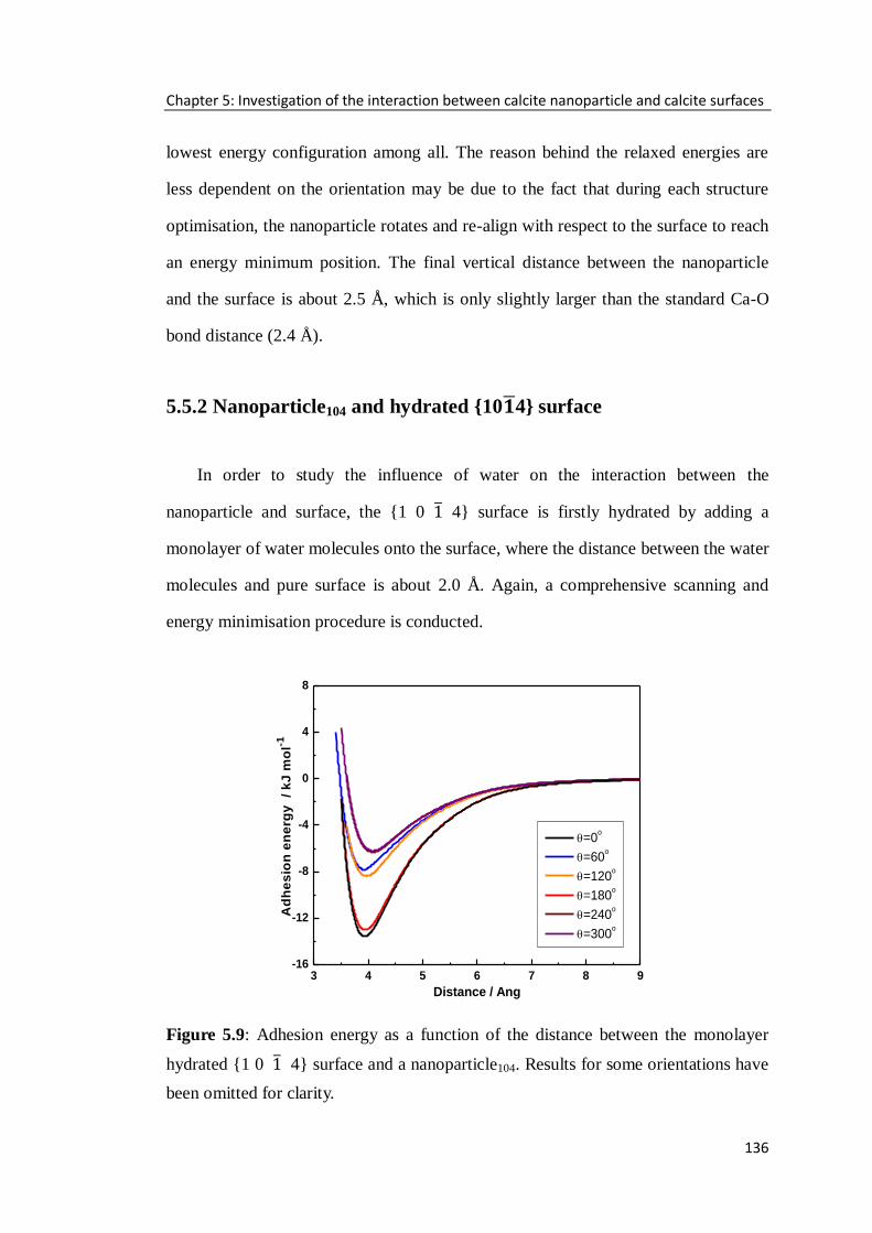
Chapter 5: Investigation of the interaction between calcite nanoparticle and calcite surfaces
136
lowest energy configuration among all. The reason behind the relaxed energies are
less dependent on the orientation may be due to the fact that during each structure
optimisation, the nanoparticle rotates and re-align with respect to the surface to reach
an energy minimum position. The final vertical distance between the nanoparticle
and the surface is about 2.5 Å, which is only slightly larger than the standard Ca-O
bond distance (2.4 Å).
5.5.2 Nanoparticle104 and hydrated {10 4} surface
In order to study the influence of water on the interaction between the
nanoparticle and surface, the {1 0 4} surface is firstly hydrated by adding a
monolayer of water molecules onto the surface, where the distance between the water
molecules and pure surface is about 2.0 Å. Again, a comprehensive scanning and
energy minimisation procedure is conducted.
Figure 5.9: Adhesion energy as a function of the distance between the monolayer
hydrated {1 0 4} surface and a nanoparticle104. Results for some orientations have
been omitted for clarity.
3 4 5 6 7 8 9-16
-12
-8
-4
0
4
8
=0o
=60o
=120o
=180o
=240o
=300o
Ad
he
sio
n e
ne
rgy
/
kJ
mo
l-1
Distance / Ang

Chapter 5: Investigation of the interaction between calcite nanoparticle and calcite surfaces
137
It is found that the general character of the plots of the energy vs. height is
similar to those obtained in vacuum, but all the plots reach their lowest values when
the nanoparticle is about 4.0 Å away from the surface regardless of the orientation of
the nanoparticle (see Figure 5.9). This is different from the pure surface, where the
location of the adhesion energy minimum varies somewhat with the orientation of
the nanoparticle.
Figure 5.10: Adhesion energy as a function of the orientation of a nanoparticle104 on
pure (black triangle) and hydrated (red circle) {1 0 4} surface.
Although the adhesion energies of the unrelaxed hydrated systems are less
dependent on the orientation compared to the pure {1 0 4} interfacial system, as
shown in Figure 5.10, the 0o rotation still remains the energetically most favourable
interfacial configuration. All these observations could be explained by the fact that
the monolayer of water molecules has unified the surface structure, which makes the
system less sensitive to the position of the nanoparticle. It is also notable that both
unrelaxed and relaxed adhesion energies of the hydrated systems (see Table 5.3 and
5.4) are less negative than those of the corresponding pure systems. For example, in
0 60 120 180 240 300 360-60
-50
-40
-30
-20
-10
0
Ad
he
sio
n e
ne
rgy
/ k
Jm
ol-1
Rotation angle / degree

Chapter 5: Investigation of the interaction between calcite nanoparticle and calcite surfaces
138
the case of a rotation of 0o, the adhesion energy has lessened by more than 50% (85.8
kJmol-1
) compared to that of the corresponding pure system, indicating that the
interfacial water layer reduces the interaction between the nanoparticle104 and the
surface.
Figure 5.11(a) has demonstrated that the energy surface of the monolayer
hydrated {10 4} interfacial system is much smoother than that of the pure surface at
a rotation of 0o. Further analysis indicated that the location of the strong interaction
positions has changed compared to the corresponding pure system, namely, the CO32-
sites become relatively low energy sites while Ca2+
sites interact more weakly no
matter the rotations of the nanoparticle104, as it can be seen from Figure 5.11(b). The
reason for such a change is probably due to the involvement of water molecules.
Figure 5.11: 3-D and 2-D adhesion energy contours of the nanoparticle104 on the
hydrated {1 0 4} surface with a rotation of θ = 0o. (Ca = green, C = grey, H =
white, O = red, Owater = blue).
Figure 5.12 showed that the monolayer of water molecules act like a „screen‟,
which prevents the surface Ca2+
ions to directly interact with the CO32-
groups of the
nanoparticle, leading to significantly reduce the attractive interaction between the
surface Ca2+
ions and CO32-
groups of the nanoparticle through the intercalated water
(a) (b)

Chapter 5: Investigation of the interaction between calcite nanoparticle and calcite surfaces
139
molecule‟s oxygen atom. However, the water layer only partially blocks the
interaction way between surface CO32-
groups and the Ca2+
ions of the nanoparticle,
which makes the water layer less impact on the interaction between surface CO32-
groups and the Ca2+
ions of the nanoparticle. As a result, the overall interaction
pattern has altered.
Figure 5.12: Side view of the unrelaxed interfacial system of the monolayer hydrated
{1 0 4} surface/calcite nanoparticle104 at a rotation of 0o. (Ca = green, C = grey, O
= red, Owater = blue, H = white).
Next, the interaction between the nanoparticle104 and hydrated {1 0 4} surface
with multilayer water was examined. A complete energy scanning procedure was
carried out for double, triple and quadruple water layers, respectively, where the
nanoparticle104 is positioned at 0o rotation only. The adhesion energy surface for the
system with double layers of water is smoother than that of the monolayer hydrated
system. The energy surfaces for the hydrated system with triple and quadruple layers
of water are rough and uneven, meaning the water molecules are starting to interact
strongly with each other through hydrogen bonds.
The variation of adhesion energy of a nanoparticle104 was then investigated,
when it approaches the hydrated surface through multilayer water. Figure 5.13
Z
X
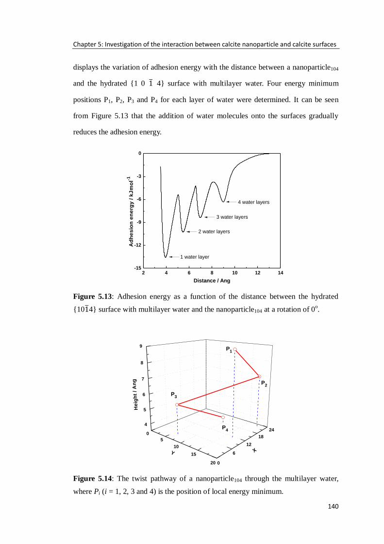
Chapter 5: Investigation of the interaction between calcite nanoparticle and calcite surfaces
140
displays the variation of adhesion energy with the distance between a nanoparticle104
and the hydrated {1 0 4} surface with multilayer water. Four energy minimum
positions P1, P2, P3 and P4 for each layer of water were determined. It can be seen
from Figure 5.13 that the addition of water molecules onto the surfaces gradually
reduces the adhesion energy.
Figure 5.13: Adhesion energy as a function of the distance between the hydrated
{10 4} surface with multilayer water and the nanoparticle104 at a rotation of 0o.
Figure 5.14: The twist pathway of a nanoparticle104 through the multilayer water,
where Pi (i = 1, 2, 3 and 4) is the position of local energy minimum.
0
5
10
15
20
4
5
6
7
8
9
0
6
12
18
24P4
P3
P2
He
igh
t /
An
g
X Y
P1
2 4 6 8 10 12 14-15
-12
-9
-6
-3
0
4 water layers
3 water layers
2 water layers
Ad
he
sio
n e
ne
rgy
/ k
Jm
ol-1
Distance / Ang
1 water layer

Chapter 5: Investigation of the interaction between calcite nanoparticle and calcite surfaces
141
The calculated results also suggest when the nanoparticle104 approaches the
{10 4} surface through the multiple water layers in a manner of a twist pathway
rather than a straight perpendicular down pathway in order to follow a energetically
favourable path, and to overcome a series of energy barriers through the water layers,
as it is illustrated in Figure 5.14 (from P1 to P4).
5.5.3 The effect of the size of a nanoparticle104
Having considered the role of the orientation of the nanoparticle on the adhesion
energy, the effect of the size of a nanoparticle on the interactions was inspected, by
considering a bigger calcite nanoparticle104 with a diameter of 1.3 nm. There are 32
CaCO3 units in this nanoparticle and 8 units in the bottom plane. Again the initial
orientation of the nanoparticle104 (θ = 0o) is assumed in the position where the lattices
of the nanoparticle104 and the {1 0 4} surface are matching perfectly. Then a
comprehensive scanning procedure on the planar {1 0 4} was carried out.
Figure 5.15: Unrelaxed adhesion energies as a function of the orientations of the
nanoparticle104 for the pure (triangle) and monolayer hydrated (circle) {1 0 4}
interfacial systems, (d = 1.0 nm: black line, d = 1.3 nm: red line).
0 60 120 180 240 300 360-80
-70
-60
-50
-40
-30
-20
-10
0
Ad
he
sio
n e
ne
rgy
/ k
Jm
ol-1
Rotation Angle degree

Chapter 5: Investigation of the interaction between calcite nanoparticle and calcite surfaces
142
The adhesion energies for the systems with a nanoparticle104 sized of 1.3 nm are
displayed in Figure 5.15, comparing with those of the smaller nanoparticle104 (d = 1.0
nm). In the case of the bigger nanoparticle104, the adhesion energies for both pure and
monolayer hydrated {1 0 4} interfacial systems are also dependent on the
orientation of the nanoparticle, which is same as the case for the smaller
nanoparticle104. The 0o and 180
o rotations still lead to the energetically most
favourable interfacial configurations.
Furthermore, the variation in the adhesion energies of the pure interfacial surface
becomes larger when the size of the nanoparticle104 increases. For example at a
rotation of 0o, the adhesion energy decreases from -55.1 kJmol
-1 to -73.5 kJmol
-1.
The reason behind these differences may be due to the stability of bigger calcite
nanoparticle104. The small nanoparticle104 can become slightly disordered due to both
rotation and translation of the under-coordinated CO32-
groups at the edge of the
particle. As the nanoparticle size increased, the influence of the fully coordinated
bulk ions begin to dominate and the long-range order in the particle increases (Cooke
and Elliott, 2007), making the lattices of the nanoparticle104 and calcite surface align
much more perfectly. Although the consideration of a bigger nanoparticle104 in the
calculations leads to much stronger interaction between the nanoparticle104 and pure
surfaces in some cases, it does not contradict our findings for the smaller
nanoparticle104, namely the adhesion energy is highly dependent on the orientation of
the nanoparticle. Moreover, the size of the nanoparticle104 does not have an apparent
effect on the adhesion energy of the hydrated {1 0 4} interfacial system (Figure
5.15). Therefore, the nanoparticle104 with a diameter of 1.0 nm has been used to
further study its interaction with other calcite surfaces.
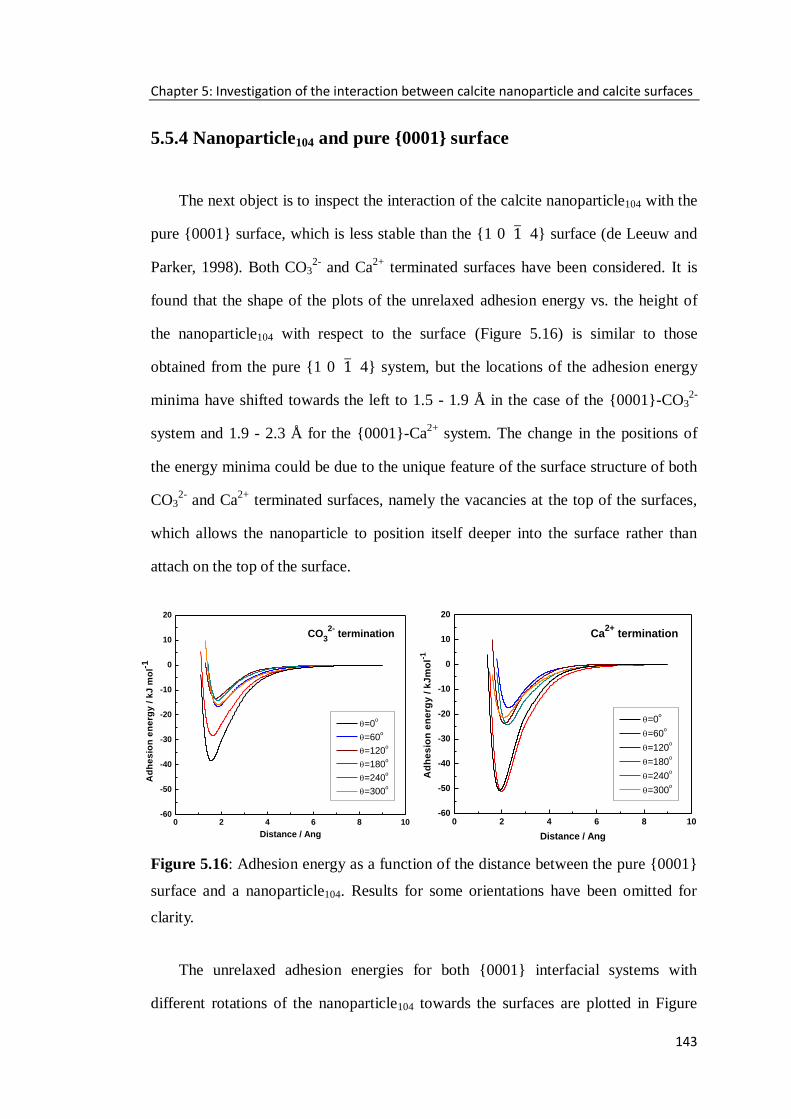
Chapter 5: Investigation of the interaction between calcite nanoparticle and calcite surfaces
143
5.5.4 Nanoparticle104 and pure {0001} surface
The next object is to inspect the interaction of the calcite nanoparticle104 with the
pure {0001} surface, which is less stable than the {1 0 4} surface (de Leeuw and
Parker, 1998). Both CO32-
and Ca2+
terminated surfaces have been considered. It is
found that the shape of the plots of the unrelaxed adhesion energy vs. the height of
the nanoparticle104 with respect to the surface (Figure 5.16) is similar to those
obtained from the pure {1 0 4} system, but the locations of the adhesion energy
minima have shifted towards the left to 1.5 - 1.9 Å in the case of the {0001}-CO32-
system and 1.9 - 2.3 Å for the {0001}-Ca2+
system. The change in the positions of
the energy minima could be due to the unique feature of the surface structure of both
CO32-
and Ca2+
terminated surfaces, namely the vacancies at the top of the surfaces,
which allows the nanoparticle to position itself deeper into the surface rather than
attach on the top of the surface.
Figure 5.16: Adhesion energy as a function of the distance between the pure {0001}
surface and a nanoparticle104. Results for some orientations have been omitted for
clarity.
The unrelaxed adhesion energies for both {0001} interfacial systems with
different rotations of the nanoparticle104 towards the surfaces are plotted in Figure
0 2 4 6 8 10-60
-50
-40
-30
-20
-10
0
10
20
Ca2+
termination
=0o
=60o
=120o
=180o
=240o
=300o
Ad
he
sio
n e
ne
rgy
/ k
Jm
ol-1
Distance / Ang
0 2 4 6 8 10-60
-50
-40
-30
-20
-10
0
10
20
=0o
=60o
=120o
=180o
=240o
=300o
Distance / Ang
A
dh
es
ion
en
erg
y /
kJ
mo
l-1
CO3
2- termination

Chapter 5: Investigation of the interaction between calcite nanoparticle and calcite surfaces
144
5.17. Like the pure {1 0 4} interfacial system, the adhesion energies of the
unrelaxed systems are highly dependent on the orientation of the nanoparticle104. It is
notable that for the {0001}-Ca2+
surface, both 0o and 180
o rotation configurations
lead to low energy configurations, although the configuration at 0o rotation is
energetically more favourable. This phenomenon has also been observed in the pure
{1 0 4} system. However, for the {0001}-CO32-
surface, the energy difference
between these two rotations is about 10.8 kJmol-1
.
Figure 5.17: Adhesion energy as a function of the orientation of a nanoparticle104 on
pure {0001} surfaces.
The reason behind the distinct difference is probably due to the fact that both
{10 4} and {0001}-Ca2+
surfaces have a similar surface atoms arrangement of
CO32-
-Ca2+
-CO32-
-Ca2+
, while for the {0001}-CO32-
surface, the arrangement has
changed to CO32-
-CO32-
-CO32-
-CO32-
. In addition, detailed structure analysis
indicated that in the case of {0001}-CO32-
surface, when the nanoparticle104 at a
rotation of 180o, the distance between the CO3
2- groups at bottom plane of the
nanoparticle104 and those CO32-
groups of the surface plane is smaller (2.84 Å)
0 60 120 180 240 300 360-60
-50
-40
-30
-20
-10
0
10
{0001}-CO32- surface
{0001}-Ca2+ surface
Ad
he
sio
n e
ne
rgy
/ k
Jm
ol-1
Rotation Angle / degree
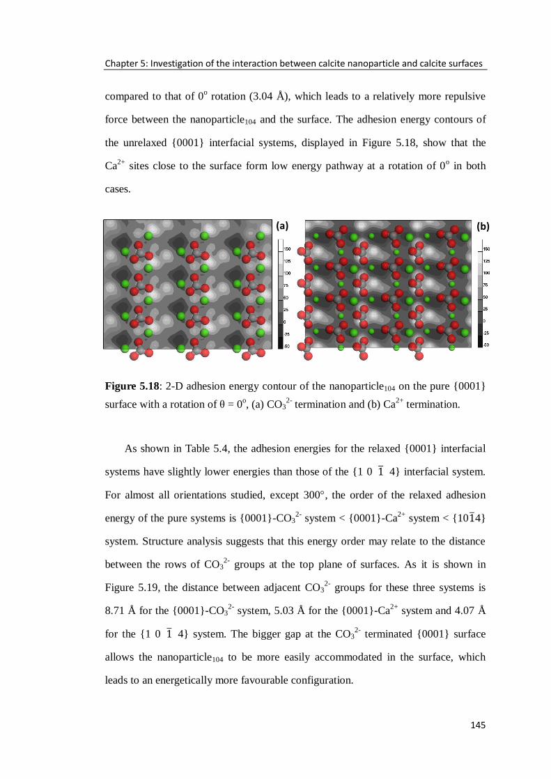
Chapter 5: Investigation of the interaction between calcite nanoparticle and calcite surfaces
145
compared to that of 0o rotation (3.04 Å), which leads to a relatively more repulsive
force between the nanoparticle104 and the surface. The adhesion energy contours of
the unrelaxed {0001} interfacial systems, displayed in Figure 5.18, show that the
Ca2+
sites close to the surface form low energy pathway at a rotation of 0o in both
cases.
Figure 5.18: 2-D adhesion energy contour of the nanoparticle104 on the pure {0001}
surface with a rotation of θ = 0o, (a) CO3
2- termination and (b) Ca
2+ termination.
As shown in Table 5.4, the adhesion energies for the relaxed {0001} interfacial
systems have slightly lower energies than those of the {1 0 4} interfacial system.
For almost all orientations studied, except 300, the order of the relaxed adhesion
energy of the pure systems is {0001}-CO32-
system < {0001}-Ca2+
system < {10 4}
system. Structure analysis suggests that this energy order may relate to the distance
between the rows of CO32-
groups at the top plane of surfaces. As it is shown in
Figure 5.19, the distance between adjacent CO32-
groups for these three systems is
8.71 Å for the {0001}-CO32-
system, 5.03 Å for the {0001}-Ca2+
system and 4.07 Å
for the {1 0 4} system. The bigger gap at the CO32-
terminated {0001} surface
allows the nanoparticle104 to be more easily accommodated in the surface, which
leads to an energetically more favourable configuration.
(a) (b)

Chapter 5: Investigation of the interaction between calcite nanoparticle and calcite surfaces
146
Figure 5.19: Side view of the top plane of (a) {0001}-CO32-
surface, (b) {0001}-Ca2+
surface and (c) {1 0 4} surface, (Ca = green, C = grey, O = red).
5.5.5 Nanoparticle104 and hydrated {0001} surface
The effect of hydration on the interaction of the {0001} interfacial systems was
then studied. The results reveal that the main feature of the curves of the unrelaxed
adhesion energy vs. the height of the nanoparticle104 with respect to the surface of
both hydrated {0001} systems has been kept but the positions of the energy minima
have changed, moving away from the surface (see Figure 5.20 for details). In the
case of the hydrated {0001}-Ca2+
interfacial systems, the adhesion energy minima
are at around 3.9 Å, e.g. very similar to those in the hydrated {1 0 4} system.
However, the adhesion energy minima for the hydrated {0001}-CO32-
systems are
located at approximately 2.8 Å, which is smaller compared to those of {0001}-Ca2+
and {1 0 4} systems. This could be attributed to the surface atom arrangement
mentioned before. The calculated results also indicate that like the monolayer
hydrated {1 0 4} system, the interaction between the nanoparticle104 and the
monolayer hydrated {0001} surfaces is weaker than those of the corresponding pure
(a)
(b)
(c)

Chapter 5: Investigation of the interaction between calcite nanoparticle and calcite surfaces
147
systems (see Table 5.3 and Table 5.4), including both relaxed and unrelaxed systems.
The strength of the interactions is relatively isotropic with the orientation of the
nanoparticle, compared to the corresponding pure systems. The rotations of 0o and
180o still lead to the energetically favourable interfacial configurations.
Figure 5.20: Adhesion energy as a function of the distance between the monolayer
hydrated {0001} surface and a nanoparticle104. Results for some orientations have
been omitted for clarity.
Figure 5.21: Adhesion energy as a function of the distance between the multilayer
hydrated {0001} surface and the nanoparticle104 at a rotation of 0o.
1 3 5 7 9 11-30
-25
-20
-15
-10
-5
0
5
10
15
=0o
=60o
=120o
=180o
=240o
=300o
Ad
he
sio
n e
ne
rgy
/ k
J m
ol-1
Distance / Ang
CO32-
termination
1 3 5 7 9 11-12
-10
-8
-6
-4
-2
0
2
4
Ca2+
termination
=0o
=60o
=120o
=180o
=240o
=300o
Ad
he
sio
n e
ne
rgy
/ k
J m
ol-1
Distance / Ang
1 3 5 7 9 11-24
-20
-16
-12
-8
-4
0
4
8
4 water layers
2 water layers
1 water layer CO3
2- termination
Ca2+
termination
Ad
he
sio
n e
ne
rgy
/ k
Jm
ol-1
Distance / Ang
1 water layer
2 water layers
3 water layers

Chapter 5: Investigation of the interaction between calcite nanoparticle and calcite surfaces
148
Like {1 0 4} system, the {0001} systems with multilayer water were also
examined, where four layers of water molecules (4 × 24) have been sequentially
added onto the surfaces layer by layer, where only the 0o rotation of nanoparticle104 is
considered. Figure 5.21 shows the variation of adhesion energy vs. the distance
between the surface and nanoparticle104 as the nanoparticle104 approaches the {0001}
surfaces through interfacial multiple water layers.
(a)
(b)
Figure 5.22: The twist pathway of a nanoparticle104 through the multilayer water,
where Pi is the position of local energy minimum, (a) {0001}-CO32-
surface, from P1
to P4; (b) {0001}-Ca2+
surface, from P1 to P3.
0
5
10
15
20
2
3
4
5
6
7
8
3
9
15
21
P4
P3
P2
He
igh
t /
An
g
XY
P1
0
5
10
15
20
2
3
4
5
6
7
8
2
8
14
20
P3
P2
He
igh
t /
An
g
X Y
P1

Chapter 5: Investigation of the interaction between calcite nanoparticle and calcite surfaces
149
The figure illustrates that there are energy barriers between the energy minima at
different heights, and the adhesion energy gradually reduce with the increasing of
water layers, as observed in the {1 0 4} interfacial system. However, there are
only three energy minima for the {0001}-Ca2+
system. This could be due to more
Ca2+
atoms from sub-layers exposure to the surface (see surface structure of
{0001}-Ca2+
surface in Figure 5.1), which results to adsorb more water molecules to
form the first layer than CO32-
terminated surface. The possible pathway of a
nanoparticle104 to approach the {0001} surface through interfacial multilayer water is
showed in Figure 5.22.
5.5.6 Nanoparticle104 and stepped surfaces
The interaction of a nanoparticle104 with two stepped surfaces, namely {3 1 8}
and {3 16} surfaces, have been considered in this part. As mentioned before,
these surfaces consist of {1 0 4} planes. The study of the interaction between a
nanoparticle104 and the planar {1 0 4} surface has indicated that the most stable
interfacial configuration occurs when the lattices of the nanoparticle104 and planar
{10 4} surface are perfectly aligned. Therefore a nanoparticle104 has been placed at a
similar position, namely, a rotation of 0o with respect to the terraces of the stepped
surfaces, which leads to the lattices of the nanoparticle aligned with those of the
terraces, as shown in Figure 5.23. However, the nanoparticle is not necessarily
aligned with the lattice of step wall in both stepped surfaces. A comprehensive
scanning procedure was then conducted, where the nanoparticle104 is allowed to
move along the x-axis and y-axis (e.g. step wall) on the terraces, as well as different
heights above the terraces. The lowest adhesion energies for both stepped surfaces
together with those of the planar {1 0 4} system are recorded in Table 5.5.

Chapter 5: Investigation of the interaction between calcite nanoparticle and calcite surfaces
150
Figure 5.23: Side view of the unrelaxed interfacial systems of a nanoparticle104 on
the pure stepped surface, (a) acute stepped {3 1 8} surface and (b) obtuse stepped
{3 16} surface, where the nanoparticle is at a rotation of 0o with respect to the
terraces of the stepped surfaces (Ca = green, O = red, C = grey).
Table 5.5: The lowest unrelaxed adhesion energy of a nanoparticle104 to the planar
{10 4} and stepped {3 1 8}, {3 16} surfaces.
surface adhesion energy (kJmol-1
)
pure {1 0 4} surface -55.1
pure {3 1 8} surface -59.6
pure {3 16} surface -57.6
hydrated {1 0 4} surface -13.7
hydrated {3 1 8} surface -11.8
hydrated {3 16} surface -13.2
The results shows that for the {3 1 8} interfacial system, the profile of
adhesion energy along the step wall (y-axis) is very similar to that of the planar
{10 4} systems (Figure 5.24), which features periodic fluctuation. The difference in
adhesion energies between two systems is fairly small (~ 4.5 kJmol-1
). These
evidences indicate that the step wall has very limited impact on the nanoparticle. The
reasons for such a result may be two folds. Firstly, the step wall is shallow and
(a) (b)
Z
X
Z
Y

Chapter 5: Investigation of the interaction between calcite nanoparticle and calcite surfaces
151
secondly, the lattice of the step wall is not perfectly aligned with that of the
nanoparticle.
Figure 5.24: The variation of adhesion energy as the nanoparticle104 moving along
the step wall of pure {3 1 8} surface (black line) and planar {1 0 4} surfaces
(red line).
Like the acute stepped {3 1 8} system, the obtuse stepped {3 16} system
also has the periodic feature of its adhesion energy profile along the y-axis. The
adhesion energy difference between the planar and the obtuse stepped systems is
even smaller (~ 2.5 kJmol-1
). The variation of adhesion energy with distance between
the nanoparticle104 and the terrace has a curvature with an energy minimum at 2.3 Å
for {3 1 8} system and 2.5 Å for {3 16} systems, which is very similar to
that of the planar {1 0 4} system (~2.5 Å). In addition, the shape of the curves is
identical to that of planar system. As indicated in Table 5.5, the order of the adhesion
energy for the pure systems studied here is {1 0 4} > {3 16} > {3 1 8}.
In other words, under vacuum conditions, calcite nanoparticle aggregation would
preferentially occur at acute stepped surface rather than obtuse stepped surface or
planar surface.
0 5 10 15 20 25 30-80
-40
0
40
80
120
160
200
Ad
he
sio
n e
ne
rgy
/ k
Jm
ol-1
Y axis

Chapter 5: Investigation of the interaction between calcite nanoparticle and calcite surfaces
152
In reality, aggregation process often takes place in aqueous solution rather than
in vacuum. It is therefore essential to take the effect of water on the process into
account. For this reason, the calculations have also been performed under the
aqueous conditions, where the stepped {3 1 8} and {3 16} surfaces were
covered by a monolayer of water molecules. A comprehensive scanning procedure
was repeated on the hydrated stepped surfaces.
It is discovered that the most stable interfacial configuration occurs when the
distance between the nanoparticle104 and terrace is at 4.2 Å for both acute surface and
obtuse surface, which is a little higher than that of the planar {1 0 4} system
(~4.0Å). The variation of adhesion energies with the distance between the
nanoparticle104 and the terrace is plotted in Figure 5.25. It is clear from the figure that
the plots have the same profile as that of hydrated planar surface (black line). The
calculated adhesion energies for the hydrated stepped surfaces are less negative than
those of the corresponding pure stepped surfaces.
Figure 5.25: Adhesion energy as a function of the height between a nanoparticle104
and the hydrated planar and stepped surfaces.
3 4 5 6 7 8 9-15
-10
-5
0
5
{1014} surface
{3148} surface
{31216} surface
Ad
he
sio
n e
ne
rgy
/ k
Jm
ol-1
Distance / Ang

Chapter 5: Investigation of the interaction between calcite nanoparticle and calcite surfaces
153
It is also very interesting to note that under aqueous condition, the order of the
adhesion energies for three systems studied has altered to {1 0 4} < {3 16}
< {3 1 8}, where the hydrated planar {1 0 4} surface becomes the most
attractive to the nanoparticle104 compared to the stepped surfaces. The main reason
for such a change may be due to the fact that the water molecules are highly ordered
and tightly bound to the planar surface in the {1 0 4} system, leading to a strong
interaction between the nanoparticle104 and the planar surface. The steps on the
obtuse {3 16} surface creates new adsorption Ca2+
sites along the step edge,
making the water molecules strongly bound to Ca2+
ions along the step edge; so the
distribution of water molecules on the terraces of the obtuse stepped surface is
similar to that of the {1 0 4}surface. However, the presence of the acute step on
the {3 1 8} surface largely affects the distribution of water molecules, especially
at the step edge, where water molecules are less ordered and a large number of the
water molecules „stand up‟ rather than „lie flat‟, as shown in Figure 5.4a. This leads
to the positively charged hydrogen atoms present on the top of acute stepped surface,
making the interaction between nanoparticle104 and the surface weaker. These results
suggest the aggregation is most likely to take place between calcite nanoparticle104
and planar surface rather than the stepped surface.
5.6 Interaction between a nanoparticle001 and calcite surface
Apart from the calcite nanoparticle104, the interaction between the calcite
surfaces and two calcite nanoparticles with {0001} surface on the outside were
considered. The diameter of the nanoparticle001-Ca is 1.0 nm and there are 12 Ca2+
atoms at the bottom, while the diameter of the nanoparticle001-CO3 is 1.2 nm and there
are 12 CO32-
groups at the bottom. The surface scanning method was used initially to
determine the interaction between the calcite nanoparticle001 and calcite planar
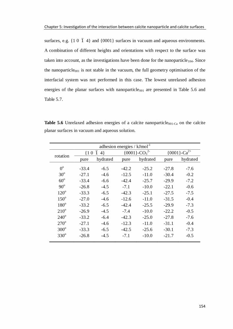
Chapter 5: Investigation of the interaction between calcite nanoparticle and calcite surfaces
154
surfaces, e.g. {1 0 4} and {0001} surfaces in vacuum and aqueous environments.
A combination of different heights and orientations with respect to the surface was
taken into account, as the investigations have been done for the nanoparticle104. Since
the nanoparticle001 is not stable in the vacuum, the full geometry optimisation of the
interfacial system was not performed in this case. The lowest unrelaxed adhesion
energies of the planar surfaces with nanoparticle001 are presented in Table 5.6 and
Table 5.7.
Table 5.6 Unrelaxed adhesion energies of a calcite nanoparticle001-Ca on the calcite
planar surfaces in vacuum and aqueous solution.
adhesion energies / kJmol-1
rotation {1 0 4} {0001}-CO3
2- {0001}-Ca
2+
pure hydrated pure hydrated pure hydrated
0o -33.4 -6.5 -42.2 -25.2 -27.8 -7.6
30o -27.1 -4.6 -12.5 -11.0 -30.4 -0.2
60o -33.4 -6.6 -42.4 -25.7 -29.9 -7.2
90o -26.8 -4.5 -7.1 -10.0 -22.1 -0.6
120o -33.3 -6.5 -42.3 -25.1 -27.5 -7.5
150o -27.0 -4.6 -12.6 -11.0 -31.5 -0.4
180o -33.2 -6.5 -42.4 -25.5 -29.9 -7.3
210o -26.9 -4.5 -7.4 -10.0 -22.2 -0.5
240o -33.2 -6.4 -42.3 -25.0 -27.8 -7.6
270o -27.1 -4.6 -12.3 -11.0 -31.1 -0.4
300o -33.3 -6.5 -42.5 -25.6 -30.1 -7.3
330o -26.8 -4.5 -7.1 -10.0 -21.7 -0.5

Chapter 5: Investigation of the interaction between calcite nanoparticle and calcite surfaces
155
Table 5.7 Unrelaxed adhesion energies of a calcite nanoparticle001-CO3 on the calcite
planar surfaces in vacuum and aqueous solution.
adhesion energies / kJmol-1
rotation {1 0 4} {0001}-CO3
2- {0001}-Ca
2+
pure hydrated pure hydrated pure hydrated
0o -10.8 -8.1 -8.4 -7.5 -9.3 -6.4
30o -5.6 -5.3 -4.2 -5.6 -6.4 -2.9
60o -6.9 -8.5 -5.9 -8.4 -8.9 -5.4
90o -6.0 -5.6 -4.9 -6.1 -6.6 -3.0
120o -10.7 -8.0 -8.4 -7.4 -9.2 -6.2
150o -5.5 -5.2 -4.2 -5.6 -6.3 -2.8
180o -6.9 -8.5 -5.8 -8.4 -8.9 -5.4
210o -6.0 -5.5 -4.9 -6.0 -6.5 -2.9
240o -10.8 -8.1 -8.3 -7.5 -9.3 -6.3
270o -5.4 -5.3 -4.2 -5.6 -6.3 -2.9
300o -6.8 -8.5 -5.9 -8.4 -8.8 -5.3
330o -6.1 -5.5 -4.7 -6.1 -6.6 -3.1
5.6.1 Nanoparticle001 and pure {10 4} surface
At first the interaction between each of the two nanoparticles001 and the pure
{10 4} surface in vacuum was investigated. The variations of the unrelaxed
adhesion energies with the height between the nanoparticle001 and the planar surface
for a various orientations are plotted in Figure 5.26. All the plots have similar
curvatures with an adhesion energy minimum at 2.4 Å of the distance between the
nanoparticle001-Ca and the {1 0 4} surface, and around 2.6 - 2.8 Å in the case of
the nanoparticle001-CO3, which are comparable to the energy minima of the
nanoparticle104 (2.5 - 2.8 Å). Although the 0o rotation leads to the energetically most
favourable interfacial configuration, the difference in adhesion energies of 0o and 30
o
rotations is only 6.3 kJmol-1
for a nanoparticle001-Ca and 5.2 kJmol-1
for a
nanoparticle001-CO3, which are much smaller than that of the nanoparticle104-{1 0 4}

Chapter 5: Investigation of the interaction between calcite nanoparticle and calcite surfaces
156
interfacial system (43.1 kJmol-1
). Unlike the nanoparticle104 interfacial system, the
unrelaxed adhesion energies are less dependent on the orientation of the
nanoparticle001.
Figure 5.26: Adhesion energy as a function of the distance between the pure {10 4}
surface and a nanoparticle001. Results for some orientations have been omitted for
clarity due to the periodic reiteration.
In general, the adhesion energy of a nanoparticle001-Ca on pure {1 0 4} surface
is more negative than that of a nanoparticle001-CO3 for each orientation studied,
meaning the positive charged nanoparticle is energetically more favourable to adhere
to the pure {1 0 4} surface than the negative charged nanoparticle. For the most
stable interfacial configuration (a rotation of 0o), the order of the adhesion energy of
a nanoparticle on the pure {1 0 4} surface is nanoparticle104 < nanoparticle001-Ca <
nanoparticle001-CO3. Further structure analysis suggests that this energy order may
relate to the bottom structure of a nanoparticle, as displayed in Figure 5.27. For a
nanoparticle104, both the rows of Ca2+
ions and CO32-
groups at the bottom of the
nanoparticle104 are aligned perfectly with the rows of CO32-
groups and Ca2+
ions of
the {1 0 4} surface. However, for a charged nanoparticle001, only the „row‟ of Ca2+
1 2 3 4 5 6 7 8 9-40
-30
-20
-10
0
10
20
30
= 0o
= 30o
Ad
he
sio
n e
ne
rgy
/
kJ
mo
l-1
Distance / Ang
Nanoparticle001-Ca
1 2 3 4 5 6 7 8 9-12
-10
-8
-6
-4
-2
0
2
4
Nanoparticle001-CO3
= 0o
= 30o
= 60o
= 90o
Ad
he
sio
n e
ne
rgy
/
kJ
mo
l-1
Distance / Ang

Chapter 5: Investigation of the interaction between calcite nanoparticle and calcite surfaces
157
ions or CO32-
groups of the nanoparticle001 is aligned with the row of CO32-
groups or
Ca2+
ions in the surface. Moreover, strong repulsive force occurs between the CO32-
groups of nanoparticle001-CO3 and the {1 0 4} surface, which largely counteracts
the attractive interaction. The periodic variation of the adhesion energy with the
orientation of a nanoparticle001-CO3 also demonstrates the effect of CO32-
groups in the
nanoparticle001-CO3 on the adhesion energy.
Figure 5.27: Side view of the most stable interfacial configurations of the pure
{10 4} surface with a calcite nanoparticle001. (a) nanoparticle001-Ca and (b)
nanoparticle001-CO3, (Ca = green; C = grey; O = red).
5.6.2 Nanoparticle001 and hydrated {10 4} surface
Subsequently, the interactions between the nanoparticle001 and the monolayer
hydrated {10 4} surface was explored. Again a comprehensive scanning procedure
was conducted. Figure 5.28 shows the plots of the adhesion energy vs. height from
the hydrated surface. The general character of these plots is similar to those obtained
in the case of the nanoparticle104. The plots of nanoparticle001-Ca reach the lowest
values at 4.0 Å regardless of the orientations; whereas the plots of nanoparticle001-CO3
have the energy minima at around 3.7 - 3.9 Å, which is a little smaller than those of
the nanoparticle104 (4.0 Å), due to the effect of hydrogen bonds formed between the
CO32-
groups in the bottom of nanoparticle001-CO3 and water molecules.
(a) (b) Z
X
Z
X

Chapter 5: Investigation of the interaction between calcite nanoparticle and calcite surfaces
158
Figure 5.28: Adhesion energy as a function of the distance between the hydrated
{10 4} surface and nanoparticle001. Results for other orientations have been omitted
for clarity.
Like the nanoparticle104, the adhesion energies of the nanoparticle001 on the
hydrated {1 0 4} surfaces are less dependent on the orientation, for example, the
energy difference between the 30o and 60
o rotations is only 2.0 kJmol
-1 for the
nanoparticle001-Ca and 3.2 kJmol-1
for the nanoparticle001-CO3. All these findings can
attribute to the fact that the monolayer water molecules have unified the surface
structure, which makes the interfacial system less sensitive to the orientations of the
nanoparticle.
It is also notable that the adhesion energy of the nanoparticle001-CO3 at each
rotation on the hydrated surface is more negative than that of the nanoparticle001-Ca,
which is opposite to the energy order for the pure systems. The reason behind this
contrary is probably due to the fact that the involvement of water molecules has not
only weaken the interaction between the surface Ca2+
ions and CO32-
groups of the
nanoparticle001-CO3, but also reduced the repulsive force between the CO32-
groups in
both the surface and the nanoparticle001-CO3. Moreover, the hydrogen bonds formed
between the oxygen in the CO32-
groups of nanoparticle001-CO3 and hydrogen atoms of
3 4 5 6 7 8 9-8
-6
-4
-2
0
2
4
6
8
Nanoparticle001-Ca
= 0o
= 30o
Ad
he
sio
n e
ne
rgy
/
kJ
mo
l-1
Distance / Ang
2 3 4 5 6 7 8 9-10
-8
-6
-4
-2
0
2
4
Nanoparticle001-CO3
= 0o
= 30o
Ad
he
sio
n e
ne
rgy
/
kJ
mo
l-1
Distance / Ang

Chapter 5: Investigation of the interaction between calcite nanoparticle and calcite surfaces
159
water molecules enhance the interaction between the nanoparticle001-CO3 and hydrated
surface, as it is illustrated in Figure 5.29.
Figure 5.29: Side view of the most stable interfacial configuration of the hydrated
{10 4} surface with a nanoparticle001-CO3 (a 0o rotation), where the blue dashes lines
show the hydrogen bonds, (Ca = green, C = grey, O = red, Owater = blue, H = white).
5.6.3 Nanoparticle001 and pure {0001} surface
The interaction of the nanoparticle001 with the pure {0001} surfaces in vacuum
are discussed in this section, where both CO32-
and Ca2+
terminated {0001} surfaces
have been considered. It is found that the shape of the plots of the unrelaxed
adhesion energy vs. the height of the nanoparticle001 with respect to the {0001}
surface has been kept, as displayed in Figure 5.30. For the nanoparticle001-CO3, the
adhesion energy minima locate at around 2.3 - 2.6 Å on the pure {0001}-Ca2+
surface and 2.4 -2.7 Å on the pure {0001}-CO32-
surface. However, for the
nanoparticle001-Ca, the adhesion energy minima have shifted towards the left to 1.5 -
2.1 Å in the case of the {0001}-Ca2+
surface, and 1.9 -2.5 Å for the {0001}-CO32-
surface. The change in the positions of the adhesion energy minima could be due to
the surface structure of {0001} surfaces. For the nanoparticle001-CO3, the strong
repulsive force occurs between the CO32-
groups at the bottom plane of the
Z
X

Chapter 5: Investigation of the interaction between calcite nanoparticle and calcite surfaces
160
nanoparticle and CO32-
groups of the {0001} surface regardless of the orientation,
which keeps the nanoparticle001-CO3 at a higher distance from the {0001} surface.
Figure 5.30: Adhesion energy as a function of the distance between a nanoparticle001
and pure {0001} surface. Results for other orientations have been omitted for clarity.
Figure 5.31 displays two stable interfacial configurations of pure {0001} surface
with a nanoparticle001-Ca at a rotation of 60o. For the {0001}-Ca
2+ surface, the “stand”
CO32-
groups in the top plane of the surface point to the Ca2+
atoms in the
nanoparticle. The distance between oxygen in the surface and Ca2+
ions in the
nanoparticle is 2.34 Å, which results to a preponderant attractive force allowing the
0 1 2 3 4 5 6 7 8-35
-25
-15
-5
5
15
= 0o
= 30o
= 60o
= 90o
Ad
he
sio
n e
ne
rgy
/
kJ
mo
l-1
Distance / Ang
nanoparticle001-Ca on Ca2+
- termination
0 1 2 3 4 5 6 7 8-50
-40
-30
-20
-10
0
10
20
30
nanoparticle001-Ca on CO32-
- termination
= 0o / 60
o
= 30o
= 90o
Ad
he
sio
n e
ne
rgy
/
kJ
mo
l-1
Distance / Ang
1 2 3 4 5 6 7 8-12
-8
-4
0
4
8
nanoparticle001-CO3 on Ca2+
- termination
= 0o
= 30o
= 60o
= 90o
Ad
he
sio
n e
ne
rgy
/
kJ
mo
l-1
Distance / Ang
1 2 3 4 5 6 7 8-12
-8
-4
0
4
8
nanoparticle001-CO3 on CO32-
- termination
= 0o
= 30o
= 60o
= 90o
Ad
he
sio
n e
ne
rgy
/
kJ
mo
l-1
Distance / Ang

Chapter 5: Investigation of the interaction between calcite nanoparticle and calcite surfaces
161
nanoparticle001-Ca to be more easily accommodated to the {0001}-Ca2+
surface.
Similarly, for the {0001}-CO32-
surface, the distance between oxygen in the surface
and Ca2+
ions in the nanoparticle is around 2.5 - 2.6 Å, which is only slightly larger
than the standard Ca - O bond distance (2.4 Å), leading to an energetically favourable
configuration.
Figure 5.31: Side view of the most stable interfacial configurations of the pure
{0001} surface with a nanoparticle001-Ca. (a) Ca2+
termination and (b) CO32-
termination, (Ca = green; C = grey; O = red).
The unrelaxed adhesion energies for both {0001} interfacial systems with
different orientations of the nanoparticle001 are illustrated in Figure 5.32. Like the
cases of the nanoparticle001 on the pure {1 0 4} surface, the adhesion energies of
(a)
(b)
Z
Y
Z
Y
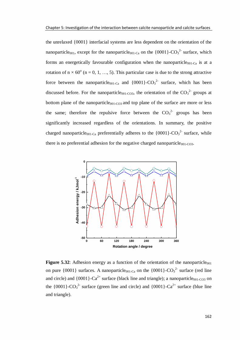
Chapter 5: Investigation of the interaction between calcite nanoparticle and calcite surfaces
162
the unrelaxed {0001} interfacial systems are less dependent on the orientation of the
nanoparticle001, except for the nanoparticle001-Ca on the {0001}-CO32-
surface, which
forms an energetically favourable configuration when the nanoparticle001-Ca is at a
rotation of n × 60o (n = 0, 1, …, 5). This particular case is due to the strong attractive
force between the nanoparticle001-Ca and {0001}-CO32-
surface, which has been
discussed before. For the nanoparticle001-CO3, the orientation of the CO32-
groups at
bottom plane of the nanoparticle001-CO3 and top plane of the surface are more or less
the same; therefore the repulsive force between the CO32-
groups has been
significantly increased regardless of the orientations. In summary, the positive
charged nanoparticle001-Ca preferentially adheres to the {0001}-CO32-
surface, while
there is no preferential adhesion for the negative charged nanoparticle001-CO3.
Figure 5.32: Adhesion energy as a function of the orientation of the nanoparticle001
on pure {0001} surfaces. A nanoparticle001-Ca on the {0001}-CO32-
surface (red line
and circle) and {0001}-Ca2+
surface (black line and triangle); a nanoparticle001-CO3 on
the {0001}-CO32-
surface (green line and circle) and {0001}-Ca2+
surface (blue line
and triangle).
0 60 120 180 240 300 360-50
-40
-30
-20
-10
0
Ad
he
sio
n e
ne
rgy
/ k
Jm
ol-1
Rotation angle / degree
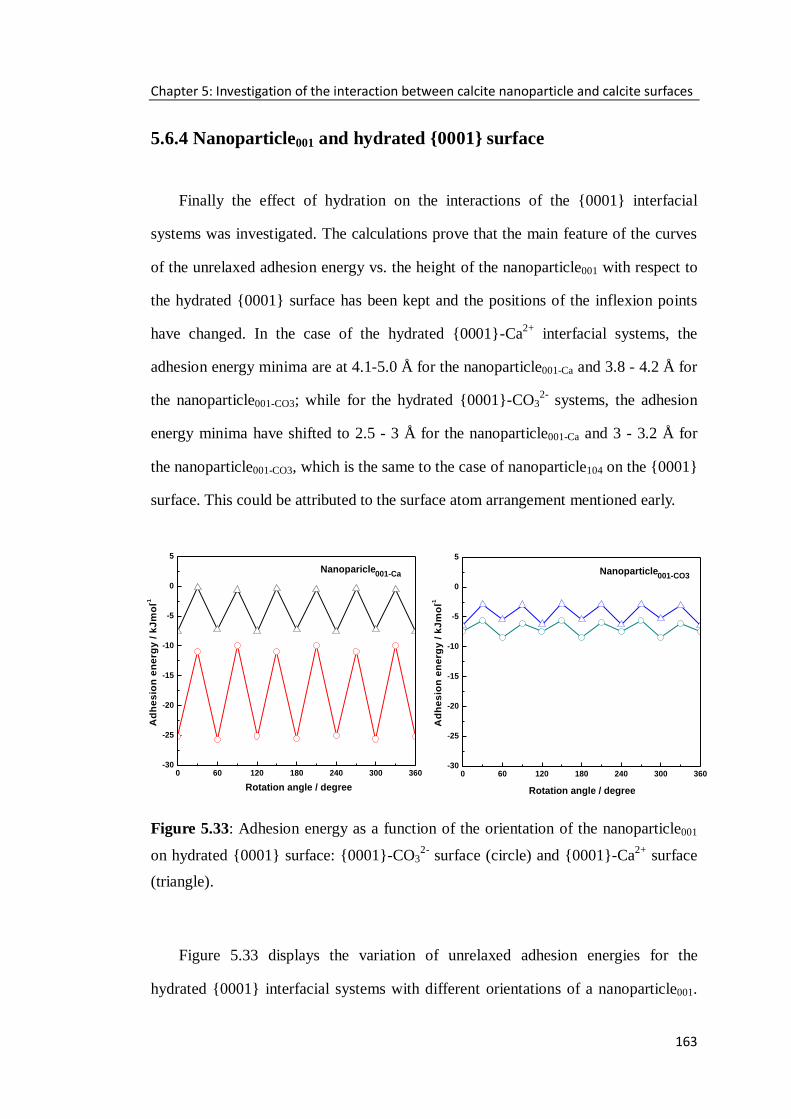
Chapter 5: Investigation of the interaction between calcite nanoparticle and calcite surfaces
163
5.6.4 Nanoparticle001 and hydrated {0001} surface
Finally the effect of hydration on the interactions of the {0001} interfacial
systems was investigated. The calculations prove that the main feature of the curves
of the unrelaxed adhesion energy vs. the height of the nanoparticle001 with respect to
the hydrated {0001} surface has been kept and the positions of the inflexion points
have changed. In the case of the hydrated {0001}-Ca2+
interfacial systems, the
adhesion energy minima are at 4.1-5.0 Å for the nanoparticle001-Ca and 3.8 - 4.2 Å for
the nanoparticle001-CO3; while for the hydrated {0001}-CO32-
systems, the adhesion
energy minima have shifted to 2.5 - 3 Å for the nanoparticle001-Ca and 3 - 3.2 Å for
the nanoparticle001-CO3, which is the same to the case of nanoparticle104 on the {0001}
surface. This could be attributed to the surface atom arrangement mentioned early.
Figure 5.33: Adhesion energy as a function of the orientation of the nanoparticle001
on hydrated {0001} surface: {0001}-CO32-
surface (circle) and {0001}-Ca2+
surface
(triangle).
Figure 5.33 displays the variation of unrelaxed adhesion energies for the
hydrated {0001} interfacial systems with different orientations of a nanoparticle001.
0 60 120 180 240 300 360-30
-25
-20
-15
-10
-5
0
5
Ad
he
sio
n e
ne
rgy
/ k
Jm
ol-1
Rotation angle / degree
Nanoparicle001-Ca
0 60 120 180 240 300 360-30
-25
-20
-15
-10
-5
0
5
Ad
he
sio
n e
ne
rgy
/ k
Jm
ol-1
Rotation angle / degree
Nanoparticle001-CO3

Chapter 5: Investigation of the interaction between calcite nanoparticle and calcite surfaces
164
In general, the adhesion energies are approximately isotropic with the orientation of
the nanoparticle001, which are similar to the pure {0001} interfacial system. Again,
the only special case is the nanoparticle001-Ca on the hydrated {0001}-CO32-
surface
(red line), where a rotation of n × 60o (n=0, 1…, 5) leads to an energetically
favourable interfacial configuration. Because the involvement of water molecules
only partially blocks the interaction way between surface CO32-
groups and the Ca2+
ions of the nanoparticle001-Ca, which makes the water layer has less impact on the
attractive force between oxygen in CO32-
group and Ca2+
ions of the nanoparticle001-Ca.
As a result, the positive charged nanoparticle001-Ca energetically prefers to adhere to
the {0001}-CO32-
surface under aqueous conditions.
5.7 Chapter summary
In this chapter, atomistic simulations techniques have been applied to investigate
the interaction of a calcite nanoparticle with the planar and stepped calcite surfaces in
both vacuum and aqueous environment, where the size, orientation and structure of
the nanoparticle have been considered.
Firstly, the size of a calcite nanoparticle has an apparent effect on the interaction
between the nanoparticle and pure surfaces. A bigger size nanoparticle leads to
stronger interaction in vacuum due to its increasing long-range order in the structure
compared to a small size nanoparticle. However, this effect on the interaction
between the nanoparticle and hydrated surface is negligible in the aqueous
environment.
Secondly, for the nanoparticle104 in vacuum, the interaction is highly dependent
on the orientation of the nanoparticle104 for both planar and stepped surfaces. The
Chapter 5: Investigation of the interaction between calcite nanoparticle and calcite surfaces
165
most stable interface occurs when the lattices of the nanoparticle and the surface are
perfectly aligned. It is energetically more favourable for the nanoparticle104 to adhere
to acute stepped {3 1 8} surface than planar {1 0 4} surface. Under aqueous
conditions, the surfaces are stabilized but energy barriers occur as the nanoparticle104
approaches the surface through the interfacial water layers. When the nanoparticle104
approaches the hydrated surface through multiple water layers, the nanoparticle will
move through a zigzag pathway rather than a direct perpendicular approach to
overcome the energy barriers. Meanwhile hydration makes the interaction of the
interfacial systems less sensitive to the orientation of the nanoparticle. Our results
also suggest that the aggregation is most likely to occur at the planar surface rather
than stepped surfaces in aqueous environment.
Finally, for the nanoparticle001, the adhesion energy is less dependent on the
orientation of the nanoparticle001 in both vacuum and aqueous environment, except
for the positive charged nanoparticle001-Ca on the {0001}-CO32-
surface. In general,
the positive charged nanoparticle001-Ca preferentially adheres to the {0001}-CO32-
surface, while there is no preferential adhesion on the planar surfaces for the negative
charged nanoparticle001-CO3.

166
6 The growth of calcium carbonate at tilt
grain boundaries and stepped surfaces
Surface defects such as steps and kinks are always present on the surfaces of
natural and synthesized nanoparticles, and the tilt grain boundaries are easy to form
between two colliding nanoparticles in aqueous environment. In this chapter
atomistic simulation techniques have been employed to investigate the structure and
stabilities of a range of tilt grain boundaries of calcite. Molecular dynamics
simulations were used next to study the growth of a series of calcium carbonates
units at the contact points of these tilt grain boundaries, which can then be used to
assess the conditions required for the inter-growth of the crystal to occur. This study
has given us the opportunity to further explore the growth mechanism of
newly-formed joints during the aggregation process of nanoparticles.

Chapter 6: The growth of calcium carbonate at tilt grain boundaries and stepped surfaces
167
6.1 Introduction
The crystallisation of calcite is one of the most important processes in the
calcium carbonate industry in determining the size and morphologies of the solid
products, which in turn affects their efficacy and applications. The calcite
nanoparticles on the scale of ~100 nm have attracted increasing attention due to their
widely applications, for example, as inorganic fillers in plastic, rubber, paper
industries and as pigments in coating and painting industries (Patton, 1979;
Schwuger, 1981; Zuiderduin et al., 2003; Gilbert and Banfield, 2005). The dispersion
of calcite nanoparticles is one of the important parameters from the viewpoint of
technical applications and influences the properties of composite materials. As a
filler material, the use of dispersive calcite nanoparticles may yield composite with
perfect strength and smoothness (Chan et al., 2002). For this reason, researchers are
working overtime to chemically modify or otherwise force calcite nanoparticles not
to aggregate or agglomerate.
When two nanoparticles collide in a suspension, hydrodynamic forces hold them
together for a short time, before attempting to pull them apart. In a supersaturated
solution, the nanoparticle will grow and new material will be deposited at the
particle/particle interface. If the growth of the nanoparticle is fast and the
hydrodynamic forces are weak, the nanoparticles will remain bound together to form
an aggregate rather than being separated by the fluid shear forces (Collier et al.,
2000). Therefore, the investigation of the growth of new calcium carbonate at the
particle/particle interface at the atomic level is essential to gain further understanding
of the aggregation of calcite nanoparticles.

Chapter 6: The growth of calcium carbonate at tilt grain boundaries and stepped surfaces
168
Although the perfect cleavage face {1 0 4} is the most stable surface of
calcite and dominates the observed morphology, the natural and synthesized surfaces
are rarely perfect or planar at the atomic scale. They always have defects such as
steps and kinks. Indeed, calcite growth and dissolution are usually found to occur
through steps and dislocations because of dangling bonds and local disorder (Putnis,
1992; Larsen et al., 2010). When two calcite nanoparticles collide in solution, the
different surfaces join together and form a grain boundary; the new CaCO3 units will
then grow at these interfaces.
The grain boundary is the interface between two grains or crystallites in a
polycrystalline material. They are the defects in the crystal structure and tend to
decrease the electrical and thermal conductivity of the material. It is convenient to
separate the grain boundaries by the extent of the mis-orientation between the two
grains. A tilt grain boundary is that where the rotation axis is parallel to the boundary
plane. An alternative is a twist grain boundary where the mis-orientation occurs
around an axis that is perpendicular to the grain boundary planes.
In this chapter a number of symmetric tilt grain boundaries of calcite containing
the acute and obtuse steps are modelled, which have been studied extensively both
experimentally and theoretically (de Leeuw, 2002; Kristensen et al., 2004; Stack and
Grantham, 2010; Larsen et al., 2010). The tilt grain boundaries are meant to act as
models of two particles, after collision has occurred but before growth has had a
chance to commence. The aim of this study is to investigate the structure and
stability of these tilt grain boundaries of calcite. Also the growth of a series of CaCO3
units at different sites present on the steps in the tilt grain boundaries, to assess the
conditions required for the growth of new CaCO3 material.

Chapter 6: The growth of calcium carbonate at tilt grain boundaries and stepped surfaces
169
6.2 Methods
Atomistic simulation techniques are employed to model the geometries and
energies of the tilt grain boundaries, which consist of large number of atoms. At first
METADISE (Watson et al., 1996) was used to create the stepped {3 1 8} and
{3 16} surfaces, both of which contain {1 0 4} planes. The steps on the {31 8}
surface are acute and the angle between the step wall and the terrace is 80º on the
relaxed surface, whereas the steps on the {3 16} surface are obtuse with an
angle of 105º between the step wall and the terrace. In order to form meaningful tilt
grain boundaries, three different size stepped surfaces for each step direction have
been modelled by gradually increasing the terrace area from 620.9 Å2 to 931.3 Å
2
and 1241.8 Å2 with the same step wall to terrace ratio.
The stepped surfaces were then used to generate the tilt grain boundaries through
the following procedure. The grain boundary was created by mirroring two identical
unrelaxed stepped surface blocks (3,456 CaCO3 units) leaving a gap of 2.0 Å
between them. The resulting structure was then allowed to relax by MD simulations
until the energy settled down. DL_POLY 2.0 (Forester and Smith, 1995) was used for
MD simulations of the grain boundaries. The equilibration of the pure system was
achieved using NVE, NVT and NPT ensembles in sequence at 300 K for 150 ps with
a time step of 0.2 fs. The final data collection simulations were run at NST for
another 100 ps. The integration algorithms are based around the Verlet Leap-Frog
scheme (Verlet, 1967) and the Nosé-Hoover algorithm (Nosé, 1984; Hoover, 1985) is
used for the thermostat. The parameter of the thermostat was set at 0.1 ps and the
barostat relaxation time was set at 0.5 ps.
During MD simulations, the movable grain blocks tend to approach each other
where there is a favourable interaction and the most stable grain boundary
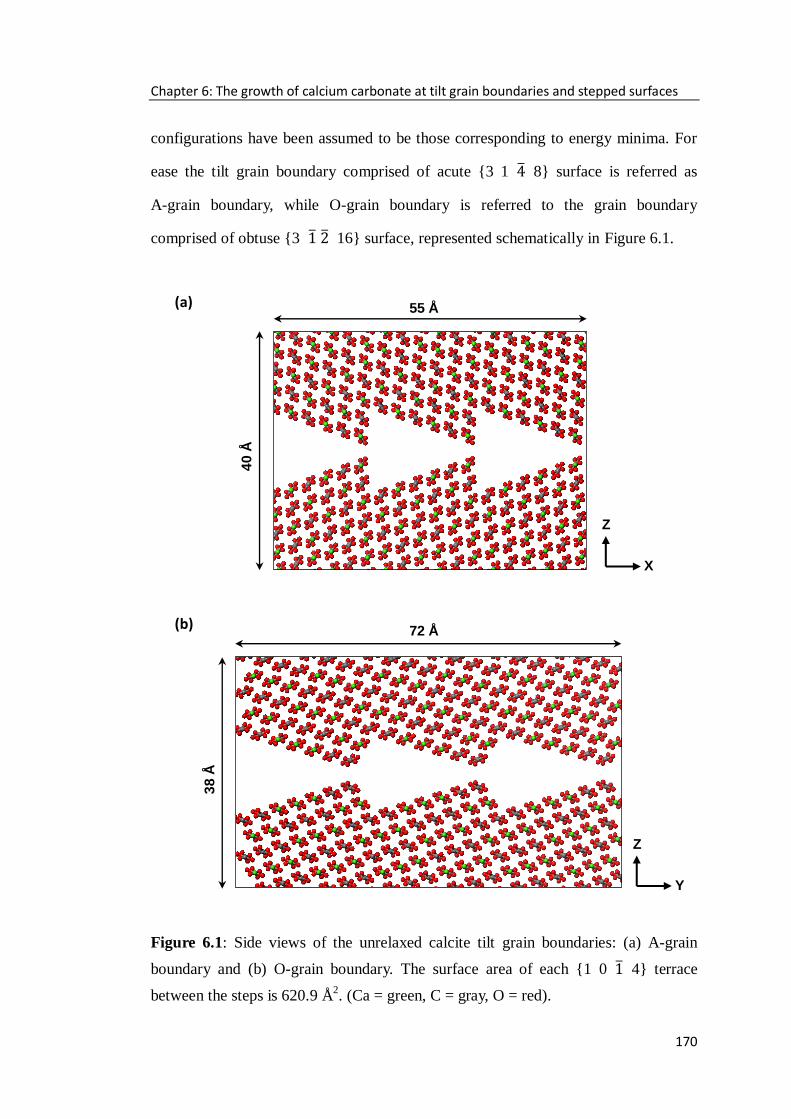
Chapter 6: The growth of calcium carbonate at tilt grain boundaries and stepped surfaces
170
configurations have been assumed to be those corresponding to energy minima. For
ease the tilt grain boundary comprised of acute {3 1 8} surface is referred as
A-grain boundary, while O-grain boundary is referred to the grain boundary
comprised of obtuse {3 16} surface, represented schematically in Figure 6.1.
(a)
(b)
Figure 6.1: Side views of the unrelaxed calcite tilt grain boundaries: (a) A-grain
boundary and (b) O-grain boundary. The surface area of each {1 0 4} terrace
between the steps is 620.9 Å2. (Ca = green, C = gray, O = red).
72 Å
55 Å
38
Å
40
Å
Z
X
Z
Y

Chapter 6: The growth of calcium carbonate at tilt grain boundaries and stepped surfaces
171
To compare the relative stability of different grain boundaries, two energy
contributions are considered here: the grain boundary energy γgrain and the cleavage
energy γcleav. The grain boundary energy is a measure of the thermodynamic stability
of a grain boundary with respect to the bulk crystal. The cleavage energy is the
energy required to cleave along the grain boundary to create two stepped surfaces
and is a measure of the stability of the grain boundary with respect to the surfaces.
These energies have been calculated for each grain boundary by using equations 6.1
and 6.2, respectively.
grain bulk
grain
U U
A
, (6.1)
2 surface grain
cleav
U U
A
. (6.2)
where Ugrain is the energy of the tilt grain boundary block, Ubulk is the energy of equal
number of atoms in the bulk structure, Usurface is the energy of the stepped surface
and A is the surface area.
For the hydrated grain boundaries, the boundary energies γhydr were calculated
with respect to liquid water and bulk crystal:
( )hydr grain bulk water
hydr
U U mU
A
(6.3)
where Uhydr-grain is the energy of the hydrated grain boundary block, Uwater is the
energy of a liquid water molecule and m is the number of water molecules. Then the
hydration energy can be obtained by comparison of the hydrated with the pure grain
boundaries and water molecules as follows:
1[ ( )]hydration hydr grain grain waterU U U mU
m (6.4)

Chapter 6: The growth of calcium carbonate at tilt grain boundaries and stepped surfaces
172
The growth of CaCO3 unit in the grain boundary systems was also studied using
MD simulations. For the addition of CaCO3 unit at various sites of the grain
boundaries in vacuum, the average growth energy per CaCO3 unit, Ugrowth, was
calculated according to the following equation:
3( )growth grain unbound grain grain CaCOU U U U U U (6.5)
where U'grain and Uunbound are the energies of the states with CaCO3 unit incorporated
and far from the stepped surface respectively. As the latter state is difficult to achieve
in reasonably sized simulation cells, its energy can be expressed as the sum of the
energy of the grain boundary and the average energy of an isolated CaCO3 unit.
For the grain boundaries in aqueous solutions, the average growth energy per
CaCO3 unit Ugrowth was calculated using the following equation:
3( )growth hydr grain hydr grain aqueous CaCOU U U U
(6.6)
where U'hydr-grain is the average energy of the grain boundary with the CaCO3 unit
incorporated under aqueous conditions, and Uaqueous-CaCO3 is the energy of the
aqueous CaCO3 unit.
6.3 Tilt grain boundaries of calcite
All the tilt grain boundaries form a series of open channels in the interfacial
region with the acute or obtuse angles between the identical step walls and terraces
preserved, for example, Figure 6.2 shows the quadrilateral channel voids formed in
the interfacial region of tilt grain boundaries with a terrace area of 1241.8 Å2. For the
A-grain boundary, the mirror step walls form an obtuse angle of 160o while the

Chapter 6: The growth of calcium carbonate at tilt grain boundaries and stepped surfaces
173
terraces form an acute angle of 40o. For the O-grain boundary, these two angles are
120o and 30
o respectively.
(a) (b)
Figure 6.2: Side view of relaxed calcite grain boundaries: (a) A-grain boundary and
(b) O-grain boundary. The surface area of the {1 0 4} terrace is 1241.8 Å2. (Ca =
green, C = gray, O = red).
The boundary energies of the tilt grain boundaries created from the two stepped
surfaces are listed in Table 6.1. For both grain boundaries, the grain boundary
energies increase as the terrace area enlarges. The boundary energies of the small
terrace (620.9 Å2) are the lowest for both grain boundaries, indicating that these grain
boundaries are very stable. It is noteworthy that the boundary energies of the O-grain
boundaries are lower than those of the A-grain boundaries with a comparable terrace
area, which is consistent to the evidence from calculated stepped surface energy that
the obtuse stepped {3 16} surface (0.72 Jm-2
) is more stable than the acute
stepped {3 1 8} surface (0.88 Jm-2
).
40o 160o
80o
105o
30o
120o

Chapter 6: The growth of calcium carbonate at tilt grain boundaries and stepped surfaces
174
The cleavage energy (Table 6.1) is a measure of the stability of the grain
boundaries with respect to the stepped surfaces, where large cleavage energy
indicates that the grain boundary is more stable with respect to the surfaces. The
stable grain boundaries with the smallest terrace areas have the largest cleavage
energies, which is due to the stability of the grain boundaries. As the obtuse stepped
{3 16} surface is more stable than the acute stepped {3 1 8} surface, the
O-grain boundary is clearly also more stable than the A-grain boundary, as already
shown by the boundary energies.
Table 6.1 Boundary and cleavage energies of the non-hydrated grain boundaries.
Terrace area / Å2 Boundary energy / Jm
-2 Cleavage energy / Jm
-2
A-grain boundary
620.9 1.07 1.46
931.3 1.15 1.32
1241.8 1.31 0.84
O-grain boundary
620.9 1.02 1.74
931.3 1.04 1.49
1241.8 1.11 1.39
The grain boundaries in aqueous liquid were then modelled. A number of water
molecules were introduced in the open channels of the grain boundary by initially
setting the water density at ρ = 1.0 gcm-3
. The boundary and hydration energies of
the hydrated grain boundaries are listed in Table 6.2. For all grain boundaries, the
boundary energies follow the same trend as those of the non-hydrated grain
boundaries, with boundary energies increasing as the terrace area increases. The
hydrated grain boundaries are more stable compared to the non-hydrated grain
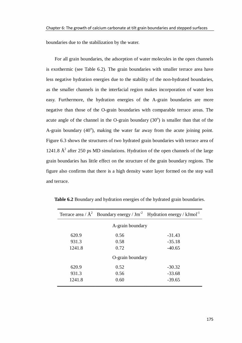
Chapter 6: The growth of calcium carbonate at tilt grain boundaries and stepped surfaces
175
boundaries due to the stabilization by the water.
For all grain boundaries, the adsorption of water molecules in the open channels
is exothermic (see Table 6.2). The grain boundaries with smaller terrace area have
less negative hydration energies due to the stability of the non-hydrated boundaries,
as the smaller channels in the interfacial region makes incorporation of water less
easy. Furthermore, the hydration energies of the A-grain boundaries are more
negative than those of the O-grain boundaries with comparable terrace areas. The
acute angle of the channel in the O-grain boundary (30o) is smaller than that of the
A-grain boundary (40o), making the water far away from the acute joining point.
Figure 6.3 shows the structures of two hydrated grain boundaries with terrace area of
1241.8 Å2 after 250 ps MD simulations. Hydration of the open channels of the large
grain boundaries has little effect on the structure of the grain boundary regions. The
figure also confirms that there is a high density water layer formed on the step wall
and terrace.
Table 6.2 Boundary and hydration energies of the hydrated grain boundaries.
Terrace area / Å2 Boundary energy / Jm
-2 Hydration energy / kJmol
-1
A-grain boundary
620.9 0.56 -31.43
931.3 0.58 -35.18
1241.8 0.72 -40.65
O-grain boundary
620.9 0.52 -30.32
931.3 0.56 -33.68
1241.8 0.60 -39.65

Chapter 6: The growth of calcium carbonate at tilt grain boundaries and stepped surfaces
176
(a)
(b)
Figure 6.3: Snapshot of hydrated grain boundaries after 250 ps MD simulations,
where four distinct Ca2+
sites are labelled in the interfacial regions. The Ca2+
in the
acute step of the joints are labelled Caa-j; the Ca2+
in the obtuse step of the joints are
labelled Cao-j; the Ca2+
at the step of original stepped surface are labelled Cac, and
Cat stands for the Ca2+
in the middle of the terraces. (a) A-grain boundary and (b)
O-grain boundary. (Ca = green, O = red, C = grey, Owater = red, H = white).
37 Å
50
Å
Z
X
Ca-c
Ca-o-j
Ca-a-j
Ca-t
44 Å
42
Å
Z
Y
Ca-c
Ca-o-j
Ca-a-j
Ca-t

Chapter 6: The growth of calcium carbonate at tilt grain boundaries and stepped surfaces
177
The structure of water around the Ca2+
ions at structurally different positions was
extracted from the radial distribution functions (RDF), obtained from the MD
simulations at 300 K, as average for 1000 configurations sampled over 100 ps of the
production run. The results are shown in Figure 6.4 and Table 6.3.
Table 6.3 Local environment of Ca2+
ions at structurally different positions in the
hydrated grain boundaries. The distance listed here are from RDF results.
Ca2+
positions Ca-Owater distance / Å Ca-Hwater distance / Å
A-grain boundary
Ca2+
(o-j) 2.49 3.29
Ca2+
(a-j) 4.20 3.39
Ca2+
(c) 4.65 4.15
Ca2+
(t) 2.39 3.19
O-grain boundary
Ca2+
(o-j) 2.49 3.29
Ca2+
(a-j) 4.95 3.59
Ca2+
(c) 4.05 3.39
Ca2+
(t) 2.43 3.29
For the Ca2+
ions within the terrace of the gain boundaries (Cat), which lack one
coordinating CO32-
compared to the Ca2+
in the bulk, one water molecule is
coordinated at an average distance of 2.39 Å in the A-grain boundary system and
2.43 Å in the O-grain boundary system. For the Ca2+
in the obtuse step of the joints
(Cao-j), which also lack one coordinating CO32-
compared to the bulk Ca2+
, one water
molecule is coordinated at a distance of 2.49 Å in both two grain boundary systems.
These Ca2+
-Owater distances match closely the experimental determination for
hydrated planar {1 0 4} surface (2.45 Å) from AFM (Ohnesorge and Binnig,
1993). This result is not surprising because a large expanse of the {1 0 4} plane is

Chapter 6: The growth of calcium carbonate at tilt grain boundaries and stepped surfaces
178
exposed to the channel voids. However, for the Ca2+
in the acute step of the joints
(Caa-j), the narrow gap can only contain limited number of water molecules, as
discussed before, making a longer Ca2+
-Owater distance at 4.20 Å for the A-grain
boundary system and 4.95 Å for the O-grain boundary system.
(a)
(b)
Figure 6.4: Radial distribution functions (RDF) for the local environment in the
water at structurally different Ca2+
surface sites. (a) A-grain boundary and (b)
O-grain boundary.
1 2 3 4 5 6 7 8 90
2
4
6
8
10
Ca2+
(o-j) - Owater
Ca2+
(a-j) - Owater
Ca2+
(c) - Owater
Ca2+
(t) - Owater
g(r
)
Distance / Ang
1 2 3 4 5 6 7 8 90
2
4
6
8
10
Ca2+
(o-j) - Owater
Ca2+
(a-j) - Owater
Ca2+
(c) - Owater
Ca2+
(t) - Owater
g(r
)
Distance / Ang

Chapter 6: The growth of calcium carbonate at tilt grain boundaries and stepped surfaces
179
It is also clear from Figure 6.3 that there are highly ordered water molecules at
the terraces of the grain boundaries. However, there is slightly disordered in the
water distribution at the steps. This fluctuation in water distribution could be highly
significant for the rate of CaCO3 growth and dissolutions, by slowing the transport of
ions and molecules to the planar terraces. We will now focus on the growth of a
series of CaCO3 units at the steps in the channel voids of the grain boundaries to
assess the conditions required for the inter-growth of CaCO3 units.
6.4 Single CaCO3 unit in aqueous environment
Theoretical investigations by Di Tommaso and de Leeuw (2008, 2009) have
shown that, although the pairing of a Ca2+
ion with a HCO3- ion in solution is
thermodynamically favourable, the subsequent addition of further Ca2+
, HCO3- or
Ca(HCO3)2 units to the first Ca2+
-HCO3- pair is endergonic. Bruneval et al. (2007),
using a combination of MD and umbrella sampling method, also showed that the
binding of Ca2+
to CO32-
in solution is strongly exothermic and there is no energy
barrier to association of these two ions. Before considering the growth of CaCO3
units at the tilt grain boundaries of calcite in solution, the formation of single CaCO3
unit in aqueous environment has been examined using classic MD simulations.
The distance between the Ca2+
and the carbon of the CO32-
in the original system
was set ~4.5 Å, and classic MD simulations were performed using the NVT
ensemble at 300 K without periodic boundary conditions. The energy of the CaCO3
group in vacuum was evaluated after equilibration. To obtain the energy of bulk
liquid water, a box containing 256 water molecules was simulated at a temperature of
300 K. The equilibration of the water simulation cell was achieved by initially setting
the experimental density at ρ = 1.0 gcm-3
and using NVE, NVT and NPT ensembles

Chapter 6: The growth of calcium carbonate at tilt grain boundaries and stepped surfaces
180
in sequence. The final data collection simulations were run in NPT ensemble. The
average energies of CaCO3 unit and liquid water at 300 K are listed in Table 6.4.
Table 6.4 Average configurational energies for the CaCO3 unit in vacuum and water,
and liquid water following simulations at 300 K for 0.2 ns.
configurational energy / eV
CaCO3 unit -52.62
bulk liquid water -9.54
aqueous CaCO3 unit -61.07
The average energy of the aqueous CaCO3 unit was calculated using a
simulation box containing 251 water molecules plus the CaCO3 unit. The simulation
box was equilibrated at NPT ensemble and 300 K for 30,000 time steps of 0.2 fs,
after which data were collected for another 70,000 time steps. Then comparing the
average energy of this simulation box with the energy of the 251 water molecules
without the dissolved CaCO3 unit gave the energy of the hydrated pair.
Figure 6.5: Representative snapshot from the MD simulations taken at 10 ps. (Ca =
green; C = grey; O = red; H = white).

Chapter 6: The growth of calcium carbonate at tilt grain boundaries and stepped surfaces
181
The configuration of the CaCO3 group in water after 10 ps is presented in Figure
6.5, which shows that the CO32-
group has replaced one water molecule in the first
coordination shell to keep a coordination number of six. This structure agrees with
the recent MD studies on the hydration structure of CaCO3 in water (Ikeda et al.,
2007; Di Tommaso and de Leeuw, 2008), which showed that the formation of the
CaCO3 monomer would occur with an associate mechanism. The hydration structure
of Ca2+
in water is highly variable as the 6-fold coordination is only marginally
preferred over the next lowest minimum, a 7-fold pentagonal bipyramidal
configurations. Figure 6.6 displays the RDFs of the Ca-Ocarbonate and Ca-Owater pairs
obtained from the MD simulations. For Ca-Ocarbonate, the first peak is at 2.28 Å,
which is 0.1 Å shorter than the average Ca-Owater distance. The results indicate that
the most stable coordination model for the aqueous CO32-
is the monodentate
configuration.
Figure 6.6: Radial distribution functions (RDF) of the Ca2+
-Ocarbonate and Ca2+
-Owater.
6.5 The growth of CaCO3 in pure grain boundary
Atomistic simulations have been employed successfully on many occasions to
model the growth and dissolution of calcite by comparing the relative
0 1 2 3 4 50
1
2
3
4
5
6
g(r
)
Distance / Ang
Ca-Owater
(b)
0 1 2 3 4 50
50
100
150
200
250
g(r
)
Distance / Ang
Ca-Ocarbonate
(a)
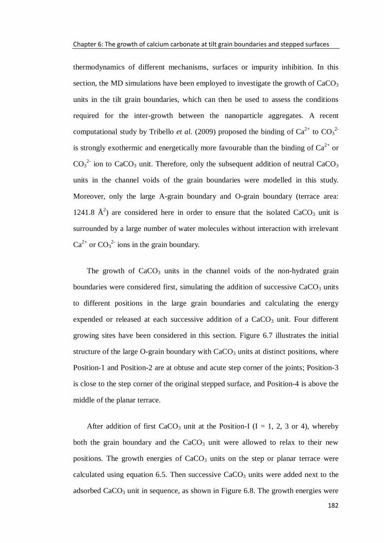
Chapter 6: The growth of calcium carbonate at tilt grain boundaries and stepped surfaces
182
thermodynamics of different mechanisms, surfaces or impurity inhibition. In this
section, the MD simulations have been employed to investigate the growth of CaCO3
units in the tilt grain boundaries, which can then be used to assess the conditions
required for the inter-growth between the nanoparticle aggregates. A recent
computational study by Tribello et al. (2009) proposed the binding of Ca2+
to CO32-
is strongly exothermic and energetically more favourable than the binding of Ca2+
or
CO32-
ion to CaCO3 unit. Therefore, only the subsequent addition of neutral CaCO3
units in the channel voids of the grain boundaries were modelled in this study.
Moreover, only the large A-grain boundary and O-grain boundary (terrace area:
1241.8 Å2) are considered here in order to ensure that the isolated CaCO3 unit is
surrounded by a large number of water molecules without interaction with irrelevant
Ca2+
or CO32-
ions in the grain boundary.
The growth of CaCO3 units in the channel voids of the non-hydrated grain
boundaries were considered first, simulating the addition of successive CaCO3 units
to different positions in the large grain boundaries and calculating the energy
expended or released at each successive addition of a CaCO3 unit. Four different
growing sites have been considered in this section. Figure 6.7 illustrates the initial
structure of the large O-grain boundary with CaCO3 units at distinct positions, where
Position-1 and Position-2 are at obtuse and acute step corner of the joints; Position-3
is close to the step corner of the original stepped surface, and Position-4 is above the
middle of the planar terrace.
After addition of first CaCO3 unit at the Position-I (I = 1, 2, 3 or 4), whereby
both the grain boundary and the CaCO3 unit were allowed to relax to their new
positions. The growth energies of CaCO3 units on the step or planar terrace were
calculated using equation 6.5. Then successive CaCO3 units were added next to the
adsorbed CaCO3 unit in sequence, as shown in Figure 6.8. The growth energies were
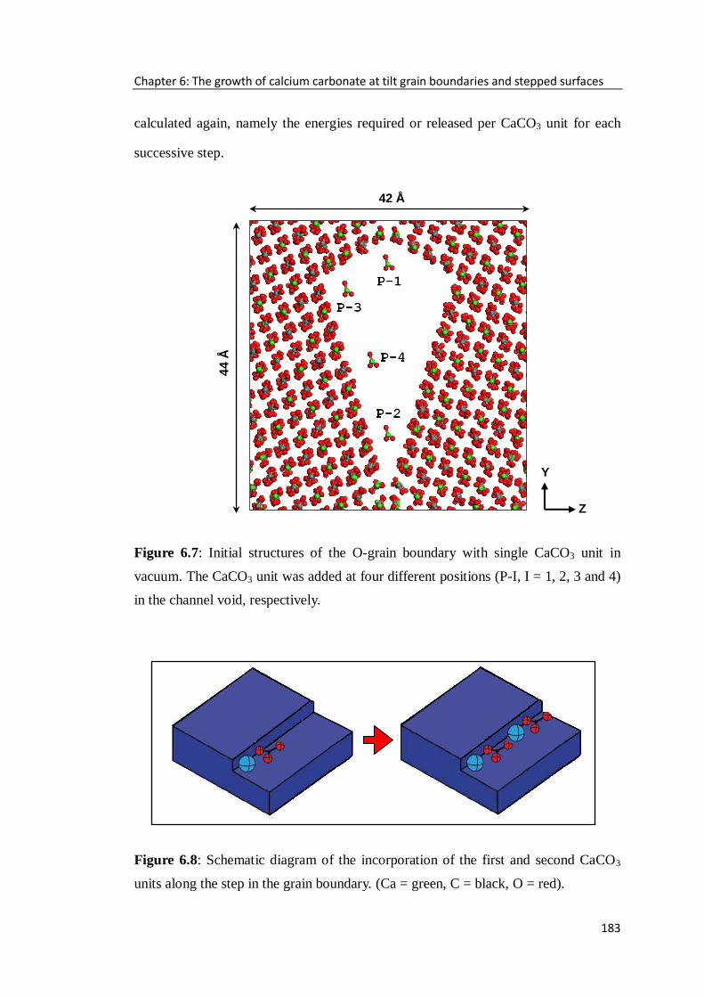
Chapter 6: The growth of calcium carbonate at tilt grain boundaries and stepped surfaces
183
calculated again, namely the energies required or released per CaCO3 unit for each
successive step.
Figure 6.7: Initial structures of the O-grain boundary with single CaCO3 unit in
vacuum. The CaCO3 unit was added at four different positions (P-I, I = 1, 2, 3 and 4)
in the channel void, respectively.
Figure 6.8: Schematic diagram of the incorporation of the first and second CaCO3
units along the step in the grain boundary. (Ca = green, C = black, O = red).
42 Å
44
Å
Y
Z

Chapter 6: The growth of calcium carbonate at tilt grain boundaries and stepped surfaces
184
Table 6.5 lists the growth energies of successive addition of CaCO3 units at
different positions in the grain boundary systems, either isolated or at kink sites next
to existing CaCO3 units. In all cases, the consecutive growth of CaCO3 units in the
grain boundaries is exothermic. Incorporation of CaCO3 units along the step is
energetically more favourable than on the planar terrace as it is much more
energetically expensive to create a “growth island” than a double kink on the surface
(Mulline, 1992). The growth of a CaCO3 unit next to an existing unit was found to be
much more energetically favourable as no new kinks were then introduced to the
steps.
Table 6.5 Growth energies of incorporation of CaCO3 units at various growth sites
on the two non-hydrated grain boundaries (kJmol-1
).
Positions Angle 1st CaCO3 2
nd CaCO3 3
rd CaCO3 4
th CaCO3
A-grain boundary
P-1 160o -310.5 -597.4 -682.4 -724.3
P-2 40o -186.8 -724.3 -772.5 -792.3
P-3 80o -219.1 -819.4 -821.0 -859.0
P-4 180o -95.4 -579.6 -621.1 -638.1
O-grain boundary
P-1 120o -301.3 -652.3 -751.1 -772.9
P-2 30o -137.1 -794.0 -824.3 -831.3
P-3 105o -244.9 -782.3 -798.4 -802.5
P-4 180o -90.3 -611.2 -635.9 -648.7
Comparing to the growth energies of CaCO3 units along the steps of the joints
(Position-1 and Position-2) in A-grain boundaries and O-grain boundaries (Figure
6.9), it shows that introduction of the first CaCO3 unit at the obtuse step (Position-1)
is much more energetically favourable than at the acute step (Position-2). When the
second CaCO3 unit was introduced at the kink sites on each step, it is energetically

Chapter 6: The growth of calcium carbonate at tilt grain boundaries and stepped surfaces
185
more favourable for further growth to occur at the acute step (Position-2) than the
obtuse step (Position-1). This tendency retains from the growth next to a kink (2nd
CaCO3) up to formation of a full step edge (4th CaCO3).
Figure 6.9: The growth energies of addition of successive CaCO3 units at the steps of
the joints (Position-1 and Position-2) in the A-grain boundary and O-grain boundary
in vacuum.
Figure 6.10 compares the average growth energies per CaCO3 unit released
when growing a complete edge of CaCO3 at various positions in the A-grain
boundary and O-grain boundary. The growth of a complete row of CaCO3 at the step
is energetically more favourable compared to consecutive addition of CaCO3 units on
the planar terrace (Position-4). A comparison of the energies of growing a full CaCO3
edge at the joints of the grain boundaries shows that larger energies are released for
the incorporation of CaCO3 at acute step (Position-2) than the obtuse step (Position-1)
in the successive growth process. Therefore, under conditions simulating ultra-high
vacuum, isolated CaCO3 unit should initially grow at the obtuse step of the joints and
1 2 3 4-1000
-800
-600
-400
-200
0
P-1 (120o) in O-grain boundary
P-1 (160o) in A-grain boundary
P-2 (30o) in O-grain boundary
P-2 (40o) in A-grain boundary
g
row
th e
ne
rgy
/ k
Jm
ol-1
CaCO3 unit

Chapter 6: The growth of calcium carbonate at tilt grain boundaries and stepped surfaces
186
then prefer to grow at the acute step of the joints. However, the growth of CaCO3 in
ultra high vacuum is not a sensible process and calcite aggregation and growth occur
under aqueous conditions. It is therefore needed to consider the effects of water in
this process.
Figure 6.10: Bar charts of the average growth energies per CaCO3 unit released upon
the growth of a full CaCO3 row in the A-grain boundary and O-grain boundary.
6.6 The growth of CaCO3 in hydrated grain boundaries
Under aqueous conditions, the channel voids of the grain boundaries were filled
with a number of water molecules to keep the water density at ρ = 1.0 gcm-3
at 300 K.
Again, four different positions have been investigated, the same as the cases of pure
grain boundaries in vacuum. After addition of each CaCO3 unit and removal of
relevant water molecules in the grain boundary system, a full MD simulation was
then performed. The growth energy of CaCO3 units at isolated positions at three steps
and planar terrace were calculated using equation 6.6, introducing kinks on each step,
and also next to the adsorbed units, are listed in Table 6.6.
-400
-500
-600
-700
-800
P- 4
P- 3P- 2
A-Grain Boundary
O-Grain Boundary
Av
era
ge
gro
wth
en
erg
y /
kJ
mo
l-1
Positions
P-1
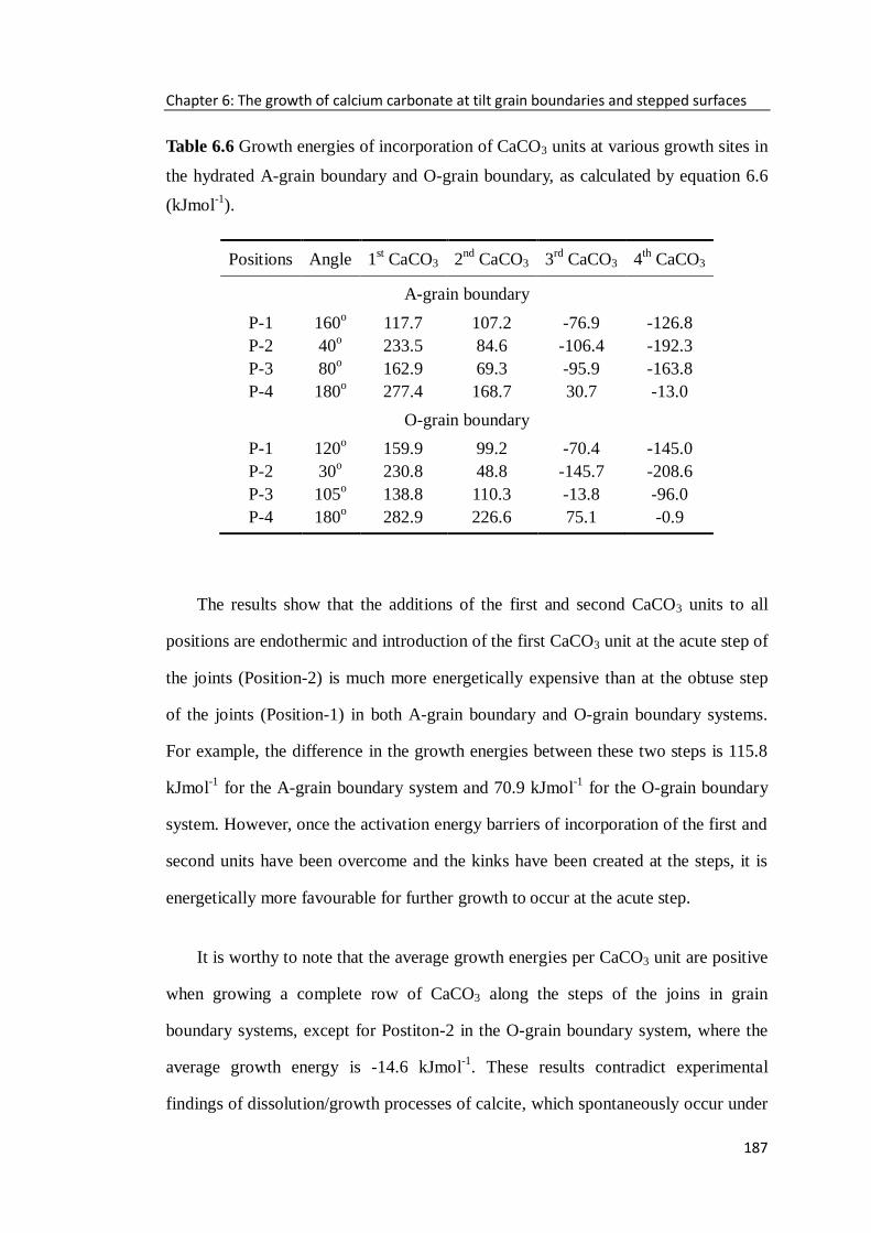
Chapter 6: The growth of calcium carbonate at tilt grain boundaries and stepped surfaces
187
Table 6.6 Growth energies of incorporation of CaCO3 units at various growth sites in
the hydrated A-grain boundary and O-grain boundary, as calculated by equation 6.6
(kJmol-1
).
Positions Angle 1st CaCO3 2
nd CaCO3 3
rd CaCO3 4
th CaCO3
A-grain boundary
P-1 160o 117.7 107.2 -76.9 -126.8
P-2 40o 233.5 84.6 -106.4 -192.3
P-3 80o 162.9 69.3 -95.9 -163.8
P-4 180o 277.4 168.7 30.7 -13.0
O-grain boundary
P-1 120o 159.9 99.2 -70.4 -145.0
P-2 30o 230.8 48.8 -145.7 -208.6
P-3 105o 138.8 110.3 -13.8 -96.0
P-4 180o 282.9 226.6 75.1 -0.9
The results show that the additions of the first and second CaCO3 units to all
positions are endothermic and introduction of the first CaCO3 unit at the acute step of
the joints (Position-2) is much more energetically expensive than at the obtuse step
of the joints (Position-1) in both A-grain boundary and O-grain boundary systems.
For example, the difference in the growth energies between these two steps is 115.8
kJmol-1
for the A-grain boundary system and 70.9 kJmol-1
for the O-grain boundary
system. However, once the activation energy barriers of incorporation of the first and
second units have been overcome and the kinks have been created at the steps, it is
energetically more favourable for further growth to occur at the acute step.
It is worthy to note that the average growth energies per CaCO3 unit are positive
when growing a complete row of CaCO3 along the steps of the joins in grain
boundary systems, except for Postiton-2 in the O-grain boundary system, where the
average growth energy is -14.6 kJmol-1
. These results contradict experimental
findings of dissolution/growth processes of calcite, which spontaneously occur under

Chapter 6: The growth of calcium carbonate at tilt grain boundaries and stepped surfaces
188
aqueous conditions (Gratz et al., 1993; Stack and Grantham, 2010).
It is possible that the calculated growth energy is affected by the energy of the
isolated aqueous CaCO3 unit far from the grain boundary in equation 6.6. Therefore
we have also calculated the average growth energy Ugrowth using the following
equation:
growth hydr grain hydr grain CaU U U (6.7)
where U'hydr-grain is the average energy of the grain boundary with the CaCO3 unit
incorporated under aqueous conditions, and Uhydr-grain-Ca is the energy of the grain
boundary with the single CaCO3 unit in the centre of the channel voids.
Table 6.7 Growth energies of incorporation of CaCO3 units at various growth sites in
the hydrated A-grain boundary and O-grain boundary, as calculated by equation 6.7
(kJmol-1
).
Positions Angle 1st CaCO3 2
nd CaCO3 3
rd CaCO3 4
th CaCO3
A-grain boundary
P-1 160o -107.6 -118.1 -127.4 -140.3
P-2 40o -48.0 -125.1 -146.5 -203.2
P-3 80o -56.7 -130.3 -145.8 -194.3
P-4 180o 10.9 -17.6 -33.5 -50.7
O-grain boundary
P-1 120o -81.9 -122.6 -136.7 -150.5
P-2 30o -22.8 -123.8 -165.3 -213.9
P-3 105o -71.0 -89.6 -103.7 -112.3
P-4 180o 23.5 -2.4 -18.9 -43.6
The growth energies of consecutive CaCO3 units in the hydrated grain boundary
systems are listed in Table 6.7, calculated by equation 6.7. Now the results show that

Chapter 6: The growth of calcium carbonate at tilt grain boundaries and stepped surfaces
189
initial additions of single CaCO3 units onto all positions are exothermic, except on
the planar terraces (Position-4) in both hydrated grain boundaries. As we have
discussed in the previous section, the adsorbed water molecules have a stabilizing
effect on the grain boundaries. On the planar terrace the water molecules form an
ordered layer, which is disturbed by the presence of steps, as shown in Figure 6.2.
Therefore, the initial growth of CaCO3 unit could prefer to occur at the steps rather
than at the terraces. However, once the activation energy barrier of incorporation of
the initial CaCO3 unit has been overcome, it is exothermic to further grow on the
terrace.
Figure 6.11: The energies of addition of successive CaCO3 units at the steps of the
joints (Position-1 and Position-2) in the A-grain boundary and O-grain boundary
under aqueous conditions.
The introduction of the first CaCO3 unit at the obtuse step (Position-1) is much
more energetically favourable than at the acute step (Position-2), as displayed in
Figure 6.11. For the A-grain boundary system, the growth energy of CaCO3 unit
1 2 3 4-240
-200
-160
-120
-80
-40
0
P-1 (120o) in O-grain boundary
P-1 (160o) in A-grain boundary
P-2 (30o) in O-grain boundary
P-2 (40o) in A-grain boundary
gro
wth
en
erg
y /
kJ
mo
l-1
CaCO3 unit

Chapter 6: The growth of calcium carbonate at tilt grain boundaries and stepped surfaces
190
incorporated at the obtuse step (Position-1, 160o) is 59.6 kJmol
-1 lower than that at
the acute step (Position-2, 40o), while the difference in growth energies between two
steps is 59.1 kJmol-1
for the O-grain boundary system. After the incorporation of the
first CaCO3 unit has created the kink at the step, it is energetically more favourable
for further growth to occur at the acute step (Position-2). For example, the order of
the energies of growing the 3rd and 4th CaCO3 units in the grain boundary systems is
P-2-O < P-2-A < P-1-O < P-1-A, which is same as the order of step angles. The
results demonstrate that the preferential growth of CaCO3 units at the grain
boundaries is dependent on the angle of the steps.
Figure 6.12: Bar charts of the average growth energies per CaCO3 unit released upon
the growth of a full CaCO3 row at the hydrated A-grain boundary and O-grain
boundary systems.
The average growth energies per CaCO3 unit released when growing a complete
row of CaCO3 onto the steps and terraces in the A and O grain boundaries are
illustrated in Figure 6.12. It is showed that the average growth energies of a CaCO3
unit at the acute step of the joints (Position-2) are slightly lower than at the obtuse
0
-50
-100
-150
-200
P- 4
P- 3P- 2
A-Grain Boundary
O-Grain boundary
Av
era
ge
gro
wth
en
erg
y /
kJ
mo
l-1
Positions
P- 1

Chapter 6: The growth of calcium carbonate at tilt grain boundaries and stepped surfaces
191
step of the joints (Position-1) during the successive growth process. Therefore when
the two calcite nanoparticles collide and form a grain boundary in the aqueous
solution, the growth velocities of the acute step should be higher than the obtuse step,
once the initial growth unit has been deposited.
Early theoretical studies of calcite growth and dissolution at the stepped surfaces
by de Leeuw and co-authors (1999, 2002) established that the activation energy
required to create the first kink site at the acute edge is 1.5 times higher than that at
the obtuse edge. Gratz et al. (1993) studied calcite growth at the two monomolecular
steps by in situ AFM techniques and found an obtuse: acute ratio of growth velocities
at the steps of 1.5 - 2.25 depending on the supersaturation. The ratio of activation
enthalpies for the initial growth of acute: obtuse calculated in this study is 1.3 to 2.1,
which agrees with previous computational and experimental research.
6.7 Chapter summary
In this chapter, atomistic simulation techniques have been employed to
investigate the geometry and stabilities of a range of tilt grain boundaries formed
from acute stepped {3 1 8} and obtuse stepped {3 16} surfaces of calcite.
For both A-grain boundaries and O-grain boundaries, the boundary stability
decreases as the terrace area increases. Furthermore, the O-grain boundary is more
stable than the A-grain boundary in both vacuum and liquid water.
Molecular dynamic simulations were then performed to investigate the growth of
a series of charge-neutral CaCO3 units at the large A-grain boundary and O-grain
boundary, implying supersaturation conditions. Four different growing positions in
vacuum and aqueous solution have been considered. The growth process modelled at

Chapter 6: The growth of calcium carbonate at tilt grain boundaries and stepped surfaces
192
the non-hydrated grain boundaries is highly exothermic but unrealistic. Under
aqueous conditions, the preferential growth of CaCO3 units is dependent on the angle
of the steps formed in the channel voids of the grain boundaries. The initial
incorporation of a CaCO3 unit is more preferential at the obtuse step of the joints in
the grain boundary, but it is much more energetically favourable at the acute step of
the joints when growing from a kink site. When the two calcite nanoparticles collide
and form a grain boundary in the aqueous solution, the growth velocities of the acute
step should be higher than the obtuse step, once the initial growth unit has been
deposited on the steps.

193
7 Conclusions and Future works
This chapter will summarise the findings of this computational study of calcium
carbonate and draw conclusions about the incorporation of cationic impurities in
calcite and the aggregation process of calcite nanoparticles, based on the results
presented in this thesis. Moreover, some possible directions for the future research
are presented.

Chapter 7: Conclusions and future works
194
7.1 Conclusions
A computer simulation study of calcium carbonate has been presented in this
thesis, where the incorporation of divalent cationic impurities in calcite and the
aggregation process of calcite nanoparticles have been included, using both
molecular mechanics (MM) and molecular dynamics (MD) simulations based on
interatomic potentials.
7.1.1 The incorporation of cationic impurities in calcite
Firstly, the mixing thermodynamics of calcite with a series of divalent cations
(Mg2+
, Ni2+
, Co2+
, Zn2+
, Fe2+
, Mn2+
and Cd2+
) have been investigated by the
atomistic simulation techniques, based on the calculation of all site occupancy
configurations in 2 × 2 × 1 and 3 × 3 × 1 supercells of the calcite structure. The
enthalpy of mixing, configurational entropy and free energy of mixing were then
calculated to explore the mixing behaviour for a series of carbonate solid solutions.
The results show that the lowest energy configuration for each cationic impurity
composition is always the one that maximises the homogeneity of the cations within
(0001) layers but maximises the heterogeneity across layers. A full disorder is likely
in (Cd,Ca)CO3 solid solutions at equilibrium conditions. Although the fully
disordered (Mn,Ca)CO3 solid solutions has positive configurational enthalpies of
mixing throughout the whole range of Mn2+
compositions, partial configurational
ordering generally lead to better agreement with recent experiments. Our results
indicate that the experimental “disordered” (Mn,Ca)CO3 solid solutions, which are
known to be favoured by kinetic factors, are actually not fully disordered, but contain
a higher abundance of low-energy cation arrangement than that expected from a
completely random distribution. For other divalent cations, i.e. Fe2+
, Zn2+
, Co2+
,

Chapter 7: Conclusions and future works
195
Mg2+
and Ni2+
, a great deal of cation ordering should be expected in the
corresponding solid solutions at high temperature (e.g. ~ 1900 K).
In particular, the structure and stability of the intermediate compositions (Mn/Ca
= 1) were investigated by a random sampling method. The most stable configuration
corresponds to the ordered dolomite-type structure. The ordered kutnahorite
(Mn0.5Ca0.5CO3) is metastable and becomes less stable than the fully disordered
50:50 solid solution at ~ 850 K and this disordering temperature decreases to a value
in better agreement with experiment (695 K), if a transition to a partially ordered
structure is considered.
The calculations have also revealed that the solubility of the cationic impurities
in calcite is largely related to the cationic coordination distance with oxygen, and the
solubility of the smaller cations in calcite is higher than that of Ca2+
in the other
end-member carbonates due to less elastic strain in the lattice. For the binary
carbonate solid solutions, CdCO3 and CaCO3 can form continuous stable solid
solution in the whole range of Cd2+
compositions at moderate temperatures. A
miscibility gap at Mn2+
composition 0.12 < x < 0.92 has been found in the
MnxCa1-xCO3 system. A higher abundance of cationic ordering are present in the
(Fe,Ca)CO3, (Co,Ca)CO3, (Zn,Ca)CO3, (Mg,Ca)CO3 and (Ni,Ca)CO3 systems, and
the solubility of these cations in calcite is extraordinary limited below 1000 K, which
are in good agreement with available experimental measurements.
7.1.2 The adhesion of calcite nanoparticles on calcite surfaces
The aggregation process of calcite nanoparticles has then been investigated by
atomistic simulations techniques. The adhesion of a calcite nanoparticle on some
major calcite surfaces has been studied in both vacuum and aqueous environment,

Chapter 7: Conclusions and future works
196
where the effects of size, orientation and structure of calcite nanoparticle on the
interaction between a nanoparticle and a surface have been investigated, respectively.
The results show that the size of a calcite nanoparticle has an apparent effect on
the interaction between the nanoparticle and surfaces in vacuum, but this influence
has not been found in the aqueous environment. For a nanoparticle104 in vacuum, the
interaction is highly dependent on the orientation of the nanoparticle for both planar
{1 0 4} and stepped surfaces (e.g. {3 1 8} and {3 16}). The most stable
interface occurs when the lattices of the nanoparticle and the surface are perfectly
aligned. The aggregation would preferentially occur at the acute stepped {3 1 8}
surface rather than the planar {1 0 4} surface. While in the aqueous environment,
the hydration makes the adhesion energy of the systems less sensitive to the
orientation of the nanoparticle. Meanwhile energy barriers occur as the nanoparticle
approaches the surface through the interfacial multiple water layers. When a
nanoparticle approaches the hydrated surface through multiple water layers, it will
move through a zigzag pathway rather than a straight perpendicular way to overcome
these energy barriers. It is energetically more favourable for the nanoparticle to
adhere to the planar {1 0 4} surface than the stepped surface in aqueous
environment, although the difference in adhesion energies is negligible.
The study has also been extended to consider a nanoparticle with different
structure, namely the nanoparticle001 in this thesis. The interaction between the
nanoparticle001 and calcite surfaces is less dependent on the orientation of the
nanoparticle in both vacuum and aqueous environment, except for the positive
charged nanoparticle001 on the CO32-
terminated {0001} surface. Generally, the
positive charged nanoparticle001 preferentially adheres to the CO32-
terminated {0001}
surface, while there is no preferential adhesion on the planar surfaces for the negative
charged nanoparticle001.

Chapter 7: Conclusions and future works
197
7.1.3 The growth of calcium carbonate in tilt grain boundaries
Finally, atomistic simulation techniques were employed to investigate the
geometry and stabilities of a range of tilt grain boundaries, which are meant to act as
models of two calcite nanoparticles, after collision has occurred but before growth
has had a chance to commence. The stability of the tilt grain boundary decreases as
the terrace area increases. The grain boundary generating by obtuse stepped surface,
is more stable than the grain boundary generating by acute stepped surface in both
vacuum and aqueous environment, which is consistent to the evidence form
calculated surface energy of stepped surface.
Molecular dynamic (MD) simulations were then used to investigate the growth
of a series of charge-neutral CaCO3 units at different positions in the grain boundary.
It is observed that the growth process modelled in the grain boundary in vacuum is
highly exothermic but unrealistic. Under aqueous conditions, the preferential growth
of CaCO3 units is dependent on the angle of the steps formed in the channel voids of
the grain boundary. The initial incorporation of a CaCO3 unit is preferential at the
obtuse step of the joints in the grain boundary, while it is much more energetically
favourable at the acute step of the joints when growing from a kink site. Our results
suggest that when the two calcite nanoparticles collide and form a grain boundary in
the aqueous solution, the ratio of activation enthalpies for the initial growth of a
CaCO3 unit at acute step to obtuse step is 1.3 to 2.1, Furthermore, the growth
velocities of the acute step should be higher than the obtuse step, once the initial
growth unit has been deposited on the steps, which agrees with experimental findings
and other theoretical studies.

Chapter 7: Conclusions and future works
198
7.2 Future works
Having investigated the incorporation of cationic impurities in calcite and the
aggregation process of calcite nanoparticles, this computational study of calcium
carbonate is only a start in its expansive and diversity fields and there are still much
more work to be done to gain a further understanding of this fantastic material.
One of the possible directions for the future research is to investigate the
incorporation of double various cationic impurities in calcite and predict the mixing
thermodynamics of tertiary carbonate solid solutions, for example, the
(Co,Zn,Ca)CO3 system. However, the set of potential parameters should be improved
to give a good description of both structural and strain effects in this mixed system
before considering the substitution of Co2+
and Zn2+
in calcite. Furthermore, some
divalent cations with ionic radius larger than Ca2+
usually prefer to substitute in
aragonite structure, i.e. Sr2+
, Pb2+
and Ba2+
. It is interesting to employ the same
method to investigate the aragonite-type solid solutions and compare the mixing
behaviors of these divalent cations in both calcite and aragonite.
For the aggregation of calcite nanoparticles, another future work should involve
the investigation of the interaction between a nanoparticle and calcite surfaces in
order to further investigate more complicated systems in terms of particle size and
aqueous conditions. It should also include developing and applying free
energy-based molecular dynamic simulations to study the variation of free energy
during the aggregation and growth process of calcite nanoparticles, where the
entropy of water molecules should be considered in the system.
Furthermore, impurities in a crystallization process have been found to have vast
effects on the morphology of the resulting crystal, with both possible beneficial and

Chapter 7: Conclusions and future works
199
detrimental effects for the resultant product. Modelling of growth rates and how the
presence of impurities affects the morphology of the crystal will be another
interesting research direction. Under the premise of the accurate potential parameters
for cationic impurities, it is possible to study the effect of these impurities on the
growth of calcium carbonate using molecular dynamics simulations, which could
give us the opportunity to discover the impurity inhibition mechanism under
complicated conditions.

Bibliographic
200
Bibliographic
Allen M. P. and Tildesley D. J. (1988) Computer simulation of liquids. Oxford
University Press, Oxford, UK.
Alloway B. J. (1995) Heavy Metals in Soils. Chapman and Hall, Glasgow, UK, 2nd
edition.
Andrews D. H. (1930) The relation between the Raman spectra and the structure of
organic molecules. Physical Review 36: 544-554.
Austen K. F., Wright K., Slater B. and Gale J. D. (2005) The interaction of dolomite
surfaces with metal impurities: a computer simulation study. Physical Chemistry and
Chemical Physics 7: 4150-4156.
BCCF (The British Calcium Carbonates Federation) (2007) Calcium carbonate:
modern day applications, http://www.calcium-carbonate.org.uk/index.asp.
Belcher A. M., Wu X. H., Christensen R. J., Hansma P. K., Stucky G. D. and Morse
D. E. (1996) Control of crystal phase switching and orientation by soluble mollusk
shell proteins. Nature 381: 56-58.
Benny S., Grau-Crespo R. and de Leeuw N. H. (2009) A theoretical investigation of
alpha-Fe2O3-Cr2O3 solid solutions. Physical Chemistry and Chemical Physics 11:
808-815.
Berner R. A. (1975) The role of magnesium in the crystal growth of calcite and
aragonite from seawater. Geochimica et Cosmochimica Acta 39: 489-504.
Bertaut F. (1958) Physique du cristal - le terme électrostatique de l'énergie de surface.
Comptes Rendus Chimie 246: 3447.

Bibliographic
201
Beruto D. and Giordani M. (1993) Calcite and aragonite formation from aqueous
calcium hydrogen carbonate solutions: effect of induced electromagnetic field on the
activity of CaCO3 nuclei precursors, Journal of the Chemistry Society, Faraday
Transaction 89: 2457-2461.
Bramley A. S., Hounslow M. J. and Ryall R. L. (1997) Aggregation during
precipitation from solution: kinetics for calcium oxalate monohydrated. Chemical
Engineering Science 52: 747-757.
Bruneval F., Donadio D. and Parrinello M. (2007) Molecular dynamics study of the
solvation of calcium carbonate in water. Journal of Physical Chemistry B 111:
12219-12227.
Born M., Huang K. (1954) Dynamic theory of crystal lattices, Oxford University
Press, Oxford, UK.
Buckingham A. (1938) The Classical Equation of State of Gaseous Helium, Neon
and Argon, Proceedings of the Royal Society of London. Series A, Mathematical and
Physical Sciences 168: 264-283.
Carpenter M. A. (1980) Mechanisms of exsolution in sodic pyroxenes. Contributions
to Mineralogy and Petrology 71: 289-300.
Catlow C. R. A. and Macrodt W. C. (1982) Computer Simulation of Solids. Springer
Verlag, Berlin, Germany.
Capobianco C. and Navrotsky A. (1987) Solid solution thermodynamics in CaCO3
-MnCO3. American Mineralogist 72: 312-318.
Chan C. M., Wu J. S., Li J. X. and Cheung Y. K. (2002) Polypropylene/calcium
carbonate nano composites. Polymer 43(10): 2981-2992.
Chang F. R. C., Skipper N. T. and Sposito G. (1995) Computer simulation of
interlayer molecular structure in sodium montmorillonite hydrates. Langmuir 11:
2734-2741.

Bibliographic
202
Chang L. L. Y., Howie R. A. and Zussman J. (1996) Rock-forming Minerals, 2nd
edition, Vol. 5, Non-silicates, 108-135.
Chiarello R. P., Sturchio N. C., Grace J. D., Geissbuhler P., Sorensen L. B., Likwan
Cheng L. and Xu S. (1997) Otavite-calcite solid solution formation at the calcite
water interface studied in situ by synchrotron X-ray scattering. Geochimica et
Cosmochimica Acta 61(7): 1467-1474.
Colfen H. (2003) Precipitation of carbonates: recent progress in controlled
production of complex shapes. Current Opinion in Colloid & Interface Science 8:
23-31.
Collier A. P., Hetherington C. J. D. and Hounslow M. J. (2000) Alignment
mechanisms between particles in crystalline aggregates. Journal of Crystal Growth
208: 513-519.
Cooke D. J. and Elliott J. A. (2007) Atomistic simulations of calcite nanoparticles
and their interaction with water. The Journal of Chemical Physics 127: 104706.
Cygan R. T., Wright K., Fisler D. K., Gale J. D. and Slater B. (2002) Atomistic
models of carbonate minerals: bulk and surface structures, defects, and diffusion.
Molecular Simulation 28: 475-495.
Davidson P. M. (1994) Ternary iron, magnesium, calcium carbonates: A
thermodynamic model for dolomite as an ordered derivative of calcite-structure
solutions. American Mineralogist 79: 332-339.
Davis J. A., Fuller C. C. and Cook A. D. (1987) A model for trace element sorption
processes at the calcite surface: Adsorption of Cd2+
and subsequent solid-solution
formation. Geochimica et Cosmochimica Acta 51: 1477-1490.
Davis K. J., Dove P. M. and de Yoreo J. J. (2000) The role of Mg2+
as an impurity on
calcite growth. Science 290: 1134-1137.
Davis P. K. and Navrotsky A. (1983) Quantitative correlations of deviations from
ideality in binary and pseudobinary solid solutions. Journal of Solid State Chemistry
Bibliographic
203
46: 1-22.
Deer W. A., Howie R. A. and Zussmann J. (1992) Introduction to the Rock-forming
Minerals. Longman Group UK Limited, Harlow, UK, 2nd
edition.
Didymus J. M., Mann S., Sanderson N. P., Oliver P., Heywood B. R. and
Aso-Samper E. J. (1993) Modelling biomineralization: studies on the morphology of
synthetic calcite. Springer Verlag, Tokyo, 267-271.
Di Tommaso D. and de Leeuw N. H. (2008) The onset of calcium carbonate
nucleation: A density functional theory molecular dynamics and hybrid
microsolvation continumn study. Journal of Physical Chemistry B 112: 6965-6975.
Di Tommaso D. and de Leeuw N. H. (2009) Theoretical study of the dimerization of
calcium carbonate in aqueous solution under natural water conditions. Geochimica et
Cosmochimica Acta 73: 5394-5405.
Dick B. G. and Overhauser A. W. (1958) Theory of the dielectric constants of alkali
halide crystals. Physical Review 112: 90-103.
de Leeuw N. H. and Parker S. C. (1997) Atomistic simulation of the effect of
molecular adsorption of water on the surface structure and energies of calcite
surfaces. Journal of the Chemical Society Faraday Transactions 93: 467-475.
de Leeuw N. H. and Parker S. C. (1998) Surface structure and morphology of
calcium carbonate polymorphs calcite, aragonite, and vaterite: an atomistic approach.
Journal of Physical Chemistry B 102: 2914-2922.
de Leeuw N. H., Parker S. C. and Harding J. H. (1999) Molecular dynamics
simulation of crystal dissolution from calcite steps. Physical Review B 60:
13792-13799.
de Leeuw N. H. and Parker S. C. (2000) Modeling absorption and segregation of
magnesium and cadmium ions to calcite surfaces: Introducing MgCO3 and CdCO3
potential models. Journal of Chemical Physics 112: 4326-4333.

Bibliographic
204
de Leeuw N. H. (2002) Molecular dynamics simulation of the growth inhibiting
effect of Fe2+
, Mg2+
, Cd2+
and Sr2+
on calcite crystal growth. Journal of Physical
Chemistry B 106: 5241-5249.
de Leeuw N. H. and Cooper T. G. (2003) A computer modeling study of the
inhibiting effect of organic adsorbates on calcite crystal growth. Crystal Growth and
Design 4: 123-133.
Domingo C., Garcia-Carmona J., Loste E., Fanovich A., Fraile J. and
Gomez-Morales J. (2004) Control of calcium carbonate morphology by precipitation
in compressed and supercritical carbon dioxide media. Journal of Crystal Growth
271: 268-273.
Du Z. and de Leeuw N. H. (2006) Molecular Dynamics simulations of hydration,
dissolution and nucleation processes at the α-quartz (0001) surface in liquid water.
Dalton Transactions 22: 2623-2634.
El-Korashy S. A. (2003) Studies on divalent ion uptake of transition metal cations by
calcite through crystallization and cation exchange process. Journal of Materials
Science 38: 1709-1719.
Ewald P. (1921) Die Berechnung optischer und elektrostatischer Gitterpotentiale.
Annals Physics 369: 253-287.
Fenter P., Geissbühler P., DiMasi E., Srajer G., Sorensen L. B. and Sturchio N. C.,
(2000) Surface speciation of calcite observed in situ by high resolution x-ray
reflectivity. Geochimica et Cosmochimica Acta 64(7): 1221-1228.
Fisler D. K., Gale J. D. and Cygan R. T. (2000) A shell model for the simulation of
rhombohedral carbonate minerals and their point defects. American Mineralogist 85:
217-224.
Freeman C. L., Harding J. H. and Duffy D. M. (2008) Simulations of calcite
crystallization on self-assembled monolayers. Langmuir 24: 9607-9615.
Freij S. J., Godelitsas A. and Putnis A. (2005) Crystal growth and dissolution

Bibliographic
205
processes at the calcite water interface in the presence of zinc ions. Journal of
Crystal Growth 273: 535-545.
Frye R. (1981) Calcite Group in Encyclopedia of Mineralogy. Hutchinson Ross
Publishing Company, Stroudsbourg, Pennsylvania, USA.
Gabriely I., Leu J. P. and Barzel U. S. (2008) Clinical problem-solving, back to
basics. New England Journal of Medicine 358: 1952-1956.
Gale J. D. (1997) GULP: A computer program for the symmetry-adapted simulation
of solids. Journal of the Chemical Society, Faraday Transactions 93: 629-637.
Gale J. D. and Rohl A. L. (2003) The general utility lattice program. Molecular
Simulation 29: 291-341.
Gamsjaeger H., Koenigsberger E. and Preis W. (2000) Lippmann diagrams: Theory
and application to carbonate systems. Aquatic Geochemistry 6: 119-132.
Garcia-Sanchez A. and Alvarez-Ayuso E. (2002) Sorption of Zn, Cd and Cr on
calcite. Application to purification of industrial wastewaters. Minerals Engineering
15: 539-547.
Gebauer D., Völkel A. and Cölfen H. (2008) Stable pre-nucleation calcium carbonate
clusters, Science, 322: 1819-1822.
Geissbühler P., Fenter P., DiMasi E., Srajer G., Sorenson L. B. and Sturchio N. C.,
(2004) Three-dimensional structure of the calcite-water interface by surface X-ray
scattering. Surface Science 573: 191-203.
Ghose S. K., Waychunas G. A. and Trainor T. P. (2010) Hydrated goethite (α-FeOOH)
(100) interface structure: Ordered water and surface functional groups. Geochimica
et Cosmochimica Acta 74: 1943-1953.
Gilbert B. and Banfield J. (2005) Chapter 6: Molecular-scale processes involving
nanoparticulate minerals in biogeochemical systems. Reviews in Mineralogy and
Geochemistry 59: 109-156.

Bibliographic
206
Goldsmith J. R. and Graf D. L. (1957) The system CaO-MnO-CO2: solid solution
and decomposition relations. Geochimica et Cosmochimica Acta 11: 310-334.
Goldsmith J. R. and Heard H. C. (1961) Subsolidus Phase Relations in the System
CaCO3-MgCO3. The Journal of Geology 69: 45-74.
Goldsmith J. R. and Northrop D. A. (1965) Subsolidus phase relations in the systems
CaCO3-MgCO3-CoCO3 and CaCO3-MgCO3-NiCO3. The Journal of Geology 73:
817-829.
Gratz A. J., Hillner P. E. and Hansma P. K. (1993) Step dynamics and spiral growth
on calcite. Geochimica et Cosmochimica Acta 57: 491-495.
Grau-crespo R., Hamad S., Catlow C. R. A. and de Leeuw N. H. (2007)
Symmetry-adapted configurational modelling of fractional site occupancy in solids.
Journal of Physics: Condensed Matter 19: 256201-256217.
Gutjahr A., Dabringhaus H. and Lacmann R. (1996) Studies of the growth and
dissolution kinetics of the CaCO3 polymorphs calcite and aragonite II. The influence
of divalent cation additives on the growth and dissolution rates. Journal of Crystal
Growth 158: 310-315.
Harding J. H. (1990) Computer simulation of defects in ionic solid. Reports on
Progress in Physics 53: 1403.
Hillner P. E., Manne S.; Hansma P. K. and Gratz A. J. (1993) Atomic force
microscope: a new tool for imaging crystal growth processes. Faraday Discussions
95:191-197.
Hoch A. R., Reddy M. M. and Aiken G. R. (2000) Calcite crystal growth inhibition
by humic substnaces with emphasis on hydrophobic acids from the Florida
Everglades. Geochimica et Cosmochimica Acta 65(1): 61-72.
Hochella M. F., Jr. Eggleston C. M., Elings V. B., Parks G. A., Brown G. E., Jr.
Kjoller K. K. and Wu C. M. (1989) Mineralogy in two dimensions: Scanning
tunneling microscopy of semiconducting minerals with implications for geochemical

Bibliographic
207
reactivity. American Mineralogist 74: 1233-1246.
Hockney R. W. (1970) The potential calculation and some applications. Vol. 9.
Academic Press, New York.
Hoover W. G. (1985) Canonical dynamics: equilibrium phase-space distributions.
Physical Review A 31: 1695-1697.
Ikeda T., Boero M. and Terakura K. (2007) Hydration properties of magnesium and
calcium ions from constrained first principles molecular dynamics. Journal of
Chemical Physics 127:74503.
IMA-NA (The Industrial Minerals Association - North America) (2011) Introduction
to calcium carbonate. http://www.ima-na.org/calcium-carbonate.
Järup L. (2003) Hazards of heavy metal contamination. British Medical Bulletin
68(1): 167-182.
Jensen F. (2007) Introduction to Computational Chemistry, John Wiley & Sons Ltd,
Chichester, West Sussex, UK, 2nd
edition.
Jorgensen W. L., Chandrasekhar J., Madura J. D., Impey R. W. and Klein M. L.
(1983) Comparison of simple potential functions for simulating liquid water. Journal
of Chemical Physics 79: 926-935.
Katsikopoulos P., Fernandez-Gonzalez A. and Prieto M. (2009) Precipitation and
mixing propertites of the “disorded” (Mn,Ca)CO3 solid solution. Geochimica et
Cosmochimica Acta 73: 6147-6161.
Kerisit S. and Parker S. C. (2004) Free energy of adsorption of water and calcium on
the {10 4} calcite surface. Chemical Communications 1: 52-54.
Kerisit S. and Parker S.C. (2004) Free energy of adsorption of water and metal ions
on the {10 4} Calcite Surface. Journal of the American Chemical Society 126:
10152-10161.

Bibliographic
208
Kerisit S., Cooke D. J., Spagnoli D. and Parker S. C. (2005) Molecular dynamics
simulations of the interactions between water and inorganic solids. Journal of
Materials Chemistry 15: 1454-1462.
Koparde V. N. and Cummings P. T. (2005) Molecular dynamics simulation of
titanium dioxide nanoparticle sintering. Journal of Physical Chemistry B 109:
24280-24287.
Kristensen R. and Stipp S. L. S. (2004) Modeling steps and kinks on the surface of
calcite. Journal of Chemical Physics 121: 8511-8523.
Kuriyavar S. I., Vetrivel R., Hegde S. G., Ramaswamy A. V., Chakrabarty D. and
Mahapatra S. (2000) Insights into the formation of hydroxyl ions in calcium
carbonate: temperature dependent FTIR and molecular modelling studies. Journal of
Materials Chemistry, 10: 1835-1840.
Lardge J. S. (2009) Investigation of the interaction of water with the calcite {10 4}
surface using ab-initio simulation. PhD thesis, University College London.
Larsen K., Bechgaard K. and Stipp S. L. S. (2010) Modelling spiral growth at
dislocations and determination of critical step lengths from pyramid geometries on
calcite {10 4} surfaces. Geochimica et Cosmochimica Acta 74: 558-567.
Lebron I. and Suarez D. L. (1998) Modeling calcite precipitation as affected by
PCO2 and organic ligands at 25oC. Mineralogical Magazine 62A: 864-865.
Lennard-Jones, J. E. (1924). On the Determination of Molecular Fields, Proceedings
of the Royal Society A 106: 463-477.
Liang Y., Baer D. R., McCoy J. M., Amonette J. E. and Lafemina J. P. (1996)
Dissolution kinetics at the calcite-water interface. Geochimica et Cosmochimica Acta
60: 4883-4887.
Liang Y. and Baer D. R. (1997) Anisotropic dissolution at the CaCO3 {10 4}-water
interface. Surface Science 373:275-287.

Bibliographic
209
Liang Y., Lea A. S., Baer D. R. and Engelhard M. H. (1996) Structure of the cleaved
CaCO3 {10 4} surface in an aqueous environment. Surface Science 351: 172-182.
Lieberman H. A., Lachman L. and Schwartz B. J. (1990) Pharmaceutical Dosage
Forms: Tablets. Dekker, New York, USA.
Liew T. L., Barrick J. P. and Hounslow M. J. (2003) A micro mechanical model for
the rate of aggregation during precipitation from solution. Chemical Engineering &
Technology 26: 282-285.
Lippmann F. (1980) Phase diagrams depicting aqueous solubility of binary mineral
systems. Neues Jahrbuch für Mineralogie 139: 1-25.
Mandell G. K., Rock P. A., Fink W. H. and Casey W. H. (1999) Lattice energies of
calcite structure metal carbonates III. Theoretical excess energies for solid solutions
(Ca, M)CO3 [M=Cd, Mn, or Fe]. Journal of Physics and Chemistry of Solids 60:
651-661.
Meldrum F. C. (2003) Calcium carbonate in biomineralisation and biomimetic
chemistry. International Materials Review 48: 187-224.
Mitchell P. J. and Fincham D. (1993) Shell model simulations by adiabatic dynamics.
Journal of Physics: Condensed Matter 5: 1031-1038.
Morse J. W. and Mackenzie F. T. (1990) Geochemistry of Sedimentary Carbonates.
Elsevier, Amsterdam, the Netherlands.
Morse P. M. (1929) Diatomic molecules according to the wave mechanics. II.
Vibrational levels. Physical Review 34: 57-64.
Mulline J. W. (1992) Crystallization. Butterworth-Heinmann Oxford, UK.
Murphy S. (2009) Atomistic simulation of defects and diffusion in oxides. PhD thesis,
Imperial College.
Nriagu J. O. (1980) Cadmium in the Environment, Part-I, Ecological Cycling.
Bibliographic
210
Wiley-Interscience.
Nriagu J. O. (1981) Cadmium in the Environment, Part-II, Health Effects.
Wiley-Interscience.
Ohnesorge F. and Binnig G. (1993) True atomic resolution by atomic force
microscopy through repulsive and attractive forces. Science 260: 1451-1456.
Oliver P. M., Parker S. C. and Mackrodt W. C. (1993) Computer simulation of the
morphology of NiO. Modelling and Simulation of Material Science and Engineering
1: 755-760.
Park N., Kim M., Langford S. C. and Dickinson J. T. (1996) Atomic layer wear of
single-crystal calcite in aqueous solution using scanning force microscopy. Journal
of Applied Physics 80: 2680-2686.
Pastero L., Costa E., Bruno M., Rubbo M., Sgualdino G. and Aquilano D. (2004)
Morphology of calcite (CaCO3) crystals growing from aqueous solutions in the
presence of Li+ ions. Surface behavior of the {0001} form. Crystal Growth and
Design 4: 485-490.
Patton T. C. (1979) Paint Flow and Pigment Dispersion. Wiley Press, New York, 2nd
edition.
Pavese A., Catti M., Parker S. C. and Wall A. (1996) Modelling of the thermal
dependence of structural and elastic properties of calcite, CaCO3. Physics and
Chemistry of Minerals 23: 89-93.
Pertlik F. (1986) Structure of hydrothermally synthesized cobalt carbonate and nickel
carbonate. Acta Crystallographica C 42: 4-5.
Pouget E. M., Bomans P. H. H., Goos J. A. C. M., Frederik P. M., de With G. and
Sommerdijk N. A. J. M. (2009) The Initial Stages of Template-Controlled CaCO3
Formation Revealed by Cryo-TEM, Science 323: 1455-1458.
Prieto M., Culbillas P. and Fernadez-Gonzalez A. (2003) Uptake of dissolved by

Bibliographic
211
biogenic and abiogenic aragonite: a comparison with sorption onto calcite.
Geochimica et Cosmochimica Acta 67: 3859-3869.
Putnis A. (1992) Introduction to Mineral Science. Cambridge University Press,
Cambridge. UK.
Rajam S. and Mann S. (1990) Selective stabilization of the (001) face of calcite in
the presence of lithium. Journal of Chemical Society, Chemical Communications 24:
1789-1791.
Reeder R. J. (1983) Crystal chemistry of the rhombohedral carbonates. Reviews in
Mineralogy and Geochemistry 11: 1-47.
Reeder R. J. (1996) Interaction of divalent cobalt, zinc, cadmium, and barium with
the calcite surface during layer growth. Geochimica et Cosmochimica Acta 60:
1543-1552.
Read W. T. and Shockley W. (1950) Dislocation models of crystal grain boundaries.
Physical Review 78: 275-289.
Rick S. W. (2004) A reoptimization of the five-site water potential (TIP5P) for use
with Ewald sums. Journal of Chemical Physics 120: 6085-6093.
Rieger, J., Frechen, T., Cox, G., Heckmann, W., Schmidt, C. and Thieme, J. (2007)
Precursor structures in the crystallization/precipitation processes of CaCO3 and
control of particle formation by polyelectrolytes. Faraday Discuss. 136: 265-277.
Rocha-Marisa. C. G., Silva A. H. M. F. T., Coutinho-Fernanda M. B. and Silva Ana
Lúcia N. (2005) Study of composites based on polypropylene and calcium carbonate
by experimental design. Polymer Testing 24: 1049-1053.
Rock P. A., Casey W. H., McBeach M. K. and Walling E. M. (1994) A new method
for determining Gibbs energies of formation of metal-carbonate solid solutions: 1.
The CaxCd1-xCO3(s) system at 298K and 1bar. Geochimica et Cosmochimica Acta 58:
4281-4291.

Bibliographic
212
Romanek C. S., Grossman E. L. and Morse J. W. (1992) Carbon isotopic
fractionation in synthetic aragonite and calcite: Effects of temperature and
precipitation rate. Geochimica et Cosmochimica Acta 56: 419-430.
Ruiz-Hernandez S. E., Grau-Crespo R., Ruiz-Salvador A. R. and de Leeuw N. H.,
(2010) Thermodynamistry of strontium incorporation in aragonite from atomistic
simulations. Geochimica et Cosmochimica Acta 74, 1320-1328.
Sadus R. J. (2002) Molecular Theory of Fluids: Theory, Algorithms and
Object-Orientation, Elsevier Science Press. 231.
Schwuger M. J. (1981) Anionic Surfactants, Surfactants Science Series. Vol. 11,
Marcel Dekker, New York, USA.
Shannon R. D. (1976) Revised effective ionic radii and systematic studies of
interatomic distances in halides and chalcogenides. Acta Crystallographica A 32,
751-767.
Smith W. and Forester T. R. (1996) DL_POLY: A general-purpose parallel molecular
dynamics simulation package. Journal of Molecular Graphics 14: 136-141.
Söhnel O. and Mullin J.W. (1982) Precipitation of calcium carbonate. Journal of
Crystal Growth 60: 239-250.
Spagnoli D., Allen J. P. and Parker S. C. (2011) The structure and dynamics of
hydrated and hydroxylated magnesium oxide nanoparticles. Langmuir 27:
1821-1829.
Spagnoli D., Banfield J. F. and Parker S. C. (2008) Free energy change of
aggregation of nanoparticles. Journal of Physical Chemistry C 112: 14731-14736.
Spagnoli D., Kerist S. and Parker S. C. (2006) Atomistic simulation of the free
energies of dissolution of ions from flat and stepped calcite surfaces. Journal of
Crystal Growth 294: 103-110.
Stack A. G. and Grantham M. C. (2010) Growth rate of calcite steps as a function of

Bibliographic
213
aqueous calcium to carbonate ratio: Independent attachment and detachment of
calcium and carbonate ions. Crystal Growth and Design 10: 1409-1413.
Stipp S. L. S., Eggleston C. M. and Nielsen B. S. (1994) Calcite surface structure
observed at microtopographic and molecular scales with atomic force microscopy
(AFM). Geochimica et Cosmochimica Acta 58:3023-3033.
Stipp S. L. S. and Hochella M. F. (1991) Structure and bonding environments at the
calcite surface as observed with X-ray photoelectron spectroscopy and low energy
electron diffraction. Geochimica et Cosmochimica Acta 55: 1723-1736.
Stipp S. L. S., Hochella M. F., Parks G. A. and Leckie J. O. (1992) Cd2+
uptake by
calcite, solid state diffusion, and the formation of solid-solution; Interface process
observed with near surface sensitive techniques. Geochimica et Cosmochimica Acta
56: 1941-1954.
Stipp S. L. S., Parks G. A., Nordstrom D. K. and Leckie J. O. (1993) Solubility
product constant and thermodynamic properties for synthetic otavite, CdCO3(s), and
aqueous association constants for the Cd(II)-CO2-H2O System.. Geochimica et
Cosmochimica Acta 57: 2699-2713.
Stipp S. L. S., Konnerup-Madsen J., Franzreb K., Kulik A. and Mathieu H. J. (1998)
Spontaneous movement of ions through calcite at standard temperature and pressure.
Nature 396:356-359.
Tasker P. W. (1979) The stability of ionic crystal surfaces. Journal of Physics C:
Solid State Physics 12: 4977-4983.
Tesoriero A. J. and Pankow J. F. (1995) Solid solution partitioning of Sr2+
, Ba2+
and
Cd2+
to calcite. Geochimica et Cosmochimica Acta 60: 1053-1063.
Todorov I. T., Allan N. L., Lavrentiev M. Y., Freeman C. L., Mohn C. E. and Purton
J. A. (2004) Simulation of mineral solid solutions at zero and high pressure using
lattice statics, lattice dynamics and Monte Carlo methods. Journal of Physics:
Condensed Matter 16: 2751.

Bibliographic
214
Tohda H., Tsuchiya Y., Kobayashi T., Kishiro H. and Yanagisawa T. (1994) The
Crystalline Structure of Pancreatic Calculi. Journal of Electron Microscopy 43:
57-61.
Tribello G. A., Bruneval F., Liew C. and Parrinello M. (2009) A molecular dynamics
study of the early stages of calcium carbonate growth. Journal of Physical Chemistry
B 113: 11680-11687.
Verlet L. (1967) Computer “Experiments” on classical fluids. I. Thermodynamical
properties of Lennard-Jones molecules. Physical Review 159: 98-103.
Vinograd V. L., Sluiter M. H. F. and Winkler B. (2009) Subsolidus phase relations in
the CaCO3-MgCO3 system predicted from the excess enthalpies of supercell
structures with single and double defects. Physical Review B 79: 104201-104209.
Vinograd V. L., Paulsen N., Winkler B. and van der Walle A. (2010)
Thermodynamics of mixing in the ternary rhombohedral carbonated solid solution
(CaxMgy, Mn1-x-y)CO3 from atomistic simulations. CALPHAD: Computer coupling of
phase diagrams and thermochemistry 34: 113-119.
Vinograd V. L., Winkler B., Putnis A., Gale J. D. and Sluiter M. H. F. (2006) Static
lattice energy calculations of mixing and ordering enthalpy in binary carbonate solid
solutions. Chemical Geology 225: 304-313.
Watson G. W., Kelsey E. T., de Leeuw N. H., Harris D. J. and Parker S. C. (1996)
Atomistic simulation of dislocations, surfaces and interfaces in MgO. Journal of
Chemical Society, Faraday Transactions 92: 433-438.
White D. N. J. (1997) A computationally efficient alternative to the Buckingham
potential for molecular mechanics calculations. Journal of Computer-Aided
Molecular Design 11: 517-521.
Wolf S. E., Leiterer J., Kappl M., Emmerling F. and Tremel W. (2008) Early
homogenous amorphous precursor stages of calcium carbonate and subsequent
crystal growth in levitated droplets. Journal of American Chemical Society. 130:

Bibliographic
215
12342-12347.
Wulff G. (1901) Zur Frage der Geschwindigkeit des Wachstums und der Auflösung
der Krystallflagen. Zeitschrift für Kristallographie 34: 449.
Zachara J. M., Cowan C. E. and Resch C. T. (1991) Sorption of divalent metals on
calcite. Geochimica et Cosmochimica Acta 55: 1549-1562.
Zachara J. M., Kittrick J. A. and Harsh J. B. (1988) The mechanism of Zn2+
adsorption on calcite. Geochimica et Cosmochimica Acta 52: 2281-2291.
Zhang J. and Reeder R. J. (1999) Comparative compressibilities of calcite-structure
carbonates: deviation from empirical relations. American Mineralogist 84: 861-870.
Zhang H. and Banfield J. F. (2004) Aggregation, coarsening, and phase
transformation in ZnS nanoparticles studied by molecular dynamics simulations.
Nano Letter 4(4): 713-718.
Zuiderduin W. C. J., Westzaan C., Huetink J. and Gaymans R. J. (2003) Toughening
of polypropylene with calcium carbonate particles, Polymer 44: 261-275.