Universität Karlsruhe (TH) Angewandte und Numerische MathematikForschungsuniversität · gegründet 1825

Christian Wieners

A short introduction to

Numerical Methods for Maxwell’s Equations

Exercises for the Oberwolfach Course 2008

Version of October 17, 2008

This note summarizes some selected chapters of the first part of my lecture on NumericalMethods for Maxwell’s Equations from last summer in Karlsruhe. It should provide somebackground material for the exercises in the Oberwolfach course.Parts of this note are extremely simple. The examples are designed to provide someinsight in the numerical difficulties which are inherent in Maxwell’e equations. Most effectsare demonstrated for the scalar wave equation. For more details and proofs of the resultswe refer to the references below.The methods presented here cannot successfully applied to photonics; this requires farmore analytical and numerical effort. Nevertheless, this note should explain why simplemethods do not work.Parts of the note are not finished. Please check our website

http://www.mathematik.uni-karlsruhe.de/user/~wieners/MaxwellCourse.pdf

for an updated and corrected version.

Contents

Introduction to Maxwell’s equations 3

1 Explicit numerical schemes for of the scalar wave equation 10

2 The FDTD method for Maxwell’s equations 20

3 Time-harmonic solutions and eigenfrequencies 24

References

[1] D. BOFFI, M. CONFORTI, AND L. GASTALDI, Modified edge finite elements for photonic crystals,Numerische Mathematik, 105 (2006), pp. 249–266.

[2] E. J. COX AND D. C. DOBSON, Maximizing band gaps in two-dimensional photonic crystals,SIAM J. Appl. Math., 59 (1999), pp. 2108–2120.

[3] D. C. DOBSON, J. GOPALAKRIHNAN, AND J. E. PASCIAK, An efficient method for band structurecalculations in 3d photonic crystals, J. Compt. Phys., 161 (2000), pp. 668–679.

[4] R. HIPTMAIR, Finite elements in computational electromagnetism, Acta Numerica, 7 (2002),pp. 237–339.

[5] P. JOLY, Variational methods for time-dependent wave propagation problems. Ainsworth, Mark(ed.) et al., Topics in computational wave propagation. Direct and inverse problems. Berlin:Springer. Lect. Notes Comput. Sci. Eng. 31, 201-264, 2003.

[6] A. KNYAZEV, Toward the optimal preconditioned eigensolver: locally optimal block precondi-tioned conjugate gradient method, SIAM Journal on Scientific Computing, 23 (2001), pp. 517–541.

[7] P. MONK, Finite element methods for Maxwell’s equations, Oxfort Science, 2002.

[8] P. MONK AND E. SÜLI, A convergence analysis of yee’s scheme on nonuniform grids, SIAM J.Numer. Anal., 31 (1994), pp. 393–412.

[9] A. TAFLOVE, Computational Elecrodynamics, ArchTechHouse, 1995.

2

Introduction to Maxwell’s equations

Basic principles

We consider electromagnetic waves in a region Ω ⊂ R3 with no magnetic sources, but Ωmay (partly) be filled with materials that absorb electric energy.Electro-magnetic waves are described by the following quantities:

E : Ω × [0,∞) → R3 electric field intensityH : Ω × [0,∞) → R3 magnetic field intensityD : Ω × [0,∞) → R3 electric displacementB : Ω × [0,∞) → R3 magnetic field induction

We assume that the following quantities are given:

J : Ω × [0,∞) → R3 electric current densityρ : Ω × [0,∞) → R electric charge density

We assume within this introduction that all fields are sufficiently smooth.

Physical laws

1) Faraday’s Law For all (smooth and bounded) oriented two-dimensional manifolds Ain Ω we have

∂t

∫A

B · da +∫

∂AE · d` = 0 ,

i.e., an electric field along the line ∂A induces a change of the magnetic introductionthrough the surface A.

Example Consider the square

A = (0, 1)× (0, 1)× 0

with boundary

∂A = (0, 1)× 0 × 0 ∪ 1 × 0 × 0 ∪ (0, 1)× 1 × 0 ∪ 0 × (0, 1)× 0

For determining the orientation we choose the normal vector on A

n(x) ≡

001

, x ∈ A

Then, we have

0 = ∂t

∫A

B · da +∫

∂AE · d` =

∫ 1

0

∫ 1

0∂tB(x1, x2, 0, t) ·

001

dx1 dx2

+∫ 1

0E(x1, 0, 0, t) ·

100

dx1 +∫ 1

0E(1, x2, 0, t) ·

010

dx2

+∫ 0

1E(x1, 1, 0, t) ·

−100

dx1 +∫ 0

1E(0, x2, t) ·

0−10

dx2

3

2) Ampere’s Law For all A ⊂ Ω we have

∂t

∫A

D · da−∫

∂AH · d` +

∫A

J · da = 0 ,

i.e., an electric current density J through A and a magnetic field H along ∂A induces achange of the electric displacement D.

3) Gauß’s Law for the electric field For all volumes V ⊂ Ω with piecewise smoothboundary we have∫

∂VD · da−

∫V

ρ dx = 0 ,

i.e. the flux of the electric displacement through ∂V coincides with the sources of thecharge density in V .

4) Gauß’s Law for the magnetic field For all V ⊂ Ω we have∫∂V

B · da = 0 ,

i.e., inflow and outflow of the magnetic flux are balanced (no magnetic sources).

Definition 1. The Maxwell p.d.e. are given by

∂tD −∇×H = −J ∂tB +∇× E = 0∇ ·D = ρ ∇ ·B = 0

Here, we use for a vector field u : Ω → R3 the notation

∇ =

∂1

∂2

∂3

∇ · u = div u = ∂1u1 + ∂2u2 + ∂3u3

∇× u = curlu =

∂2u3 − ∂3u2

∂3u1 − ∂1u3

∂1u2 − ∂2u1

Formally, we can derive the p.d.e. from Maxwell’s equations in integral form using thetheorems by Gauss and Stokes:

Gauß∫

Vdiv u dx =

∫∂V

u · da

Stokes∫

Acurlu da =

∫∂A

u · d`

Here, we use u · da = u · n da and u · d` = u · τd`, the normal vector field n : A −→ R3

and the tangential vector field τ : ∂A → R3 (where the orientation of ∂A is given by n).

4

Example (cont.) For the area A = (0, 1)× (0, 1)× 0 we have∫A

curlu · da =∫ 1

0

∫ 1

0

(∂1u2(x1, x2, 0)− ∂2u1(x1, x2, 0)

)dx1dx2

=∫ 1

0

(u2(1, x2, 0)

)dx2 −

∫ 1

0

(u1(x1, 1, 0)− u1(x1, 0, 0)

)dx1 =

∫∂A

u · d`

For the volume V = (0, 1)× (0, 1)× (0, 1) we have∫V

div u · dx =∫ 1

0

∫ 1

0

∫ 1

0(∂1u1 + ∂2u2 + ∂3u3)dx1dx2dx3

=∫ 1

0

∫ 1

0

(u1(1, x2, x3)− u1(0, x2, x3)

)dx2dx3 + · · · =

∫∂V

u · n da

(general areas A and volumes V can be computed by suitable diffeomorphisms and thetransformation theorem).Thus, the theorems by Gauss and Stokes give Maxwell’s equations in the form

1)∫

A(∂tB + curlE) · da = 0

2)∫

A(∂tD − curlH + J) · da = 0

3)∫

V(div D − ρ)dx = 0

4)∫V div B dx = 0

for all A and V . Since A and V are arbitrary and we assume smoothness for all fields, allintegrants vanish, i. e., the Maxwell p.d.e. hold for all x ∈ Ω.Observation: The p.d.e. provides 8 equations for 12 unknown components of B, E, D, H.Thus, the Maxwell system has to be closed by constitutive relations (material laws)

D = D(E,H)B = B(E,H)

Together, we now obtain 14 equations!

Lemma 1. A solution of Maxwell’s equations require the compatibility condition

∂tρ + div J = 0 .

Proof. We have

∂t

∫V

ρ dx = ∂t

∫∂V

D · da =∫

∂V(curlH− J) · da = −

∫V

div J dx

since∫

∂Vcurl H · da =

∫V

div(curl H) dx = 0 for closed surfaces.

In our lecture, we restrict ourselves to linear constitutive laws (linear non-dispersive mate-rials)

D(x, t) = ε(x) E(x, t)B(x, t) = µ(x)H(x, t)

5

withε : Ω → R3×3 or R electric permittivityµ : Ω → R3×3 or R magnetic permeability

In general, ε(x), µ(x) are symmetric positive definite. For isotropic materials we haveε(x), µ(x) ∈ R.In the special case of homogeneous materials we have ε(x) ≡ ε and µ(x) ≡ µ not de-pending on x ∈ Ω.This gives Maxwell’s equations for linear materials:

ε∂tE −∇×H = −J µ∂tH +∇× E = 0∇ · (εE) = ρ ∇ · (µH) = 0

Now we have 6 unknowns and 8 equations!

Lemma 2. Assume∇ ·(εE(x, 0)

)= ρ(x, 0)

∇ ·(µH(x, 0)

)= 0

for the initial values at t = 0.Then, we have for every solution of the p.d.e. system

ε∂tE −∇×H = −J

µ∂tH +∇× E = 0∂tρ +∇ · J = 0

also ∇ ·(εE) = ρ and ∇ · (µH) = 0 for all t > 0.

Proof. We have for ∇ = (∂1, ∂2, ∂3)T and any smooth vector field u = (u1, u2, u3)

∇ · (∇× u) = ∂1(∂2u3 − ∂3u2) + ∂2(∂3u− ∂1u3) + ∂3(∂1u2 − ∂2u1) = 0 .

This gives∂t

(∇ · (µH)

)= ∇ · (µ∂tH) = −∇ · (∇× E) = 0

and thus ∇ · (µH) ≡ 0 for all t > 0 as a consequence of the initial condition.Analogously, we obtain from the compatibility equation

∂t

(∇ · (εE)− ρ

)= ∇ · (∇×H− J)− ∂tρ = ∇ · (∇×H) = 0

which finally proves ∇ ·(εE) = ρ.

A further constitutive law is Ohm’s Law J = σE + Ja for given

σ : Ω → R, σ(x) > 0 conductivityJa : Ω → R3 applied current density

A special case are electro-magnetic waves in the vacuum: there, we have

ρ ≡ 0; J ≡ 0, σ ≡ 0, ε ≡ ε0, µ ≡ µ0 .

We choose physical units such that ε0 = µ0 = 1.

6

A special case for Maxwell’s equations: the wave equation

Lemma 3. Consider a homogeneous and isotropic material (i.e., the parameters ε, µ, σ ∈R are constant) without charges (i.e., ρ ≡ 0) and without applied currents (Ja ≡ 0), i.e.,

ε∂tE −∇×H = −σE µ∂tH +∇× E = 0∇ · (εE) = 0 ∇ · (µH) = 0.

Then we have

∂2t E − c2∆E +

σ

ε∂tE = 0

∂2t H− c2∆H +

σ

µ∂tH = 0

where c = 1√εµ is the wave velocity and ∆ = ∂2

1 + ∂22 + ∂2

3 is the Laplacian.

Observation: We obtain 6 decoupled (damped) scalar wave equations with coupling viathe initial conditions

E(x, 0) = E0(x) , H(x, 0) = H0(x) ,

∂tH(x, 0) = − 1µ∇× E0(x) , ∂tE(x, 0) =

1ε∇×H0(x)− σ

εE0(x)

Proof. We have for a vector field u : Ω → R3

∇×∇× u =

∂2(∂1u2 − ∂2u1)− ∂3(∂3u1 − ∂1u3)∂3(∂2u3 − ∂3u2)− ∂1(∂1u2 − ∂2u1)∂1(∂3u1 − ∂1u3)− ∂2(∂2u3 − ∂2u3)

+

∂21u1 − ∂2

1u1

∂22u2 − ∂2

2u2

∂23u3 − ∂2

3u3

=

∂1 div u−∆u1

∂2 div u−∆u2

∂3 div u−∆u3

= ∇(∇ · u)−∆u

This gives

µε∂2t E = µ∂t(∇×H− σE)

= ∇× (µ∂tH)− µσ∂tE= −∇×∇× E − µσ∂tE= −∇

(ε−1∇ · (εE)︸ ︷︷ ︸

=0

)+ ∆E − µσ∂tE .

The rest follows analogously.

Remark 4. This result is restricted to smooth solution in homogeneous media, i.e., weobtain only solutions for special cases!

7

Harmonic plane waves Consider a scalar function u : R3 → C with

Lu := ∂2t u− c2∆u + σ∂tu = 0

Make the ansatz u(x, t) = exp(i(ωt− k · x)

)with wave number k ∈ R3 and frequency ω.

We have∂t exp

(i(ωt− k · x)

)= iω exp

(i(ωt− k · x)

)∂j exp

(i(ωt− k · x)

)= −ikj exp

(i(ωt− k · x)

)This gives the dispersion relation

Lu = 0 ⇐⇒ −ω2 + c|k|2 + σiω = 0

Observation: Without damping (i.e., σ = 0) we have ω(k) = c|k| and c = ω(k)|k| .

We call a medium non-dispersive if the velocity of waves in the medium is not dependingon the frequency ω. In fact, only the vacuum is non-dispersive, but in many cases thenon-dispersive effect are neglected.

Solutions of the wave equation in 1-d We consider Ω ⊂ R and u : Ω → C with∂2

t u = c2∂2xu.

A) Travelling waves u(x, t) = F (x± ct) on Ω = R for a given function F : R → R

=⇒ ∂2t F (x± ct) = c2 F ′′(x± ct) = c2∂2

x F (x± ct)

B) Harmonic waves u(x, t) = exp(i(ωt− kx)

)on Ω = R for ω

k = c. We have

wave length λ wave number k = 2πλ

frequency f angular frequency ω = 2πf .

C) The Cauchy problem for Ω = R

∂2t u = c2∂xu u(x, 0) = u0(x) ∂tu(x, 0) = v0(x)

is explicitly solved by

u(x, t) =12(u0(x− ct) + u0(x + ct)

)+

1c

∫ x+ct

x−ctv0(y)dy

Example: u0 ≡ 0, v0(x) = δ0(x) (Delta distribution) gives

u(x, t) =

1 −ct ≤ x ≤ ct

0 else

D) For the Cauchy problem for Ω = (0, π) with homogeneous boundary conditionsu(0, t) = u(π, t) = 0 for t > 0 we make the ansatz

u(x, t) =∞∑

n=1

un(t) sin(nx)

8

This gives

∞∑n=1

u′′n(t) sin(nx) = −c2∞∑

n=1

n2un(t) sin(nx) ,

i.e., u′′n + c2n2un = 0 for t > 0. The Fourier representation of the initial values

u0(x) =∞∑

n=1

an sin(nx) v0(x) =∞∑

n=1

bn sin(nx)

give un(0) = an and u′n(0) = bn. Then we have

un(t) = an cos(cnt) +1nc

bn sin(cnt)

Problem 1 Find (analytically) the Fourier representation of the solution of the scalarwave equation for the initial values u0 ≡ 1 and v0 ≡ 0. (Note that these initial values arenot compatible with the boundary conditions for t > 0.)

Solution of Problem 1 We have

an =2π

∫ π

0sin(nx)dx =

4

nπ n odd0 n even

and bn ≡ 0. This gives

u(x, t) =∞∑

n=1an cos(cnt) sin(nx)

= 12

∞∑n=1

an

(sin(nx + nct) + sin(nx− nct)

)= 1

2

(u0(x + ct) + u0(x− ct)

)with the periodic extension of u0

u0(x) =

1 x ∈ (0, π) + 2πZ0 x ∈ πZ

−1 x ∈ (−π, 0) + 2πZ

9

1 Explicit numerical schemes for of the scalar wave equation

Let the wave velocity c > 0 be constant. Consider the second order initial value problem

∂2t u(x, t) = c2∂2

xu(x, t) , (x, t) ∈ R× Ru(x, 0) = u0(x) , ∂tu(x, 0) = v0(x) , x ∈ R

and an approximation (unj )n,j ∈ Z× Z on the regular grid (∆x)Z× (∆t)Z ⊂ R× R, where

∆x > 0 spatial mesh size, xj = j∆x

∆t > 0 time step size, tn = n∆t

Problem 2 Let g ∈ C4(R) and h > 0. Prove

∣∣g′′(x)− 1h2

(g(x− h)− 2g(x) + g(x + h)

)∣∣ ≤ h2

12max

ξ∈[x−h,x+h]

∣∣g′′′′(ξ)∣∣ .Solution of Problem 2 We have the Taylor expansion

g(x + h) = g(x) + hg′(x) +12h2g′′(x) +

16h3g′′′(x) +

124

h4g′′′′(ξ1)

g(x− h) = g(x)− hg′(x) +12h2g′′(x)− 1

6h3g′′′(x) +

124

h4g′′′′(ξ2)

with ξ1 ∈ [x, x + h], ξ2 ∈ [x− h, x]. This gives

g(x + h) + g(x− h)− 2g(x) = h2g′′(x) +124

h4(g′′′′(ξ1) + g′′′′(ξ2)

).

This motivates the following finite difference scheme: Define the initial values

u0j = u0(xj) j ∈ Z

u1j = u0

j + ∆t v0(xj) j ∈ Z

and then, for n = 1, 2, ... compute

1(∆t)2

(un+1

j − 2unj + un−1

j

)= c2 1

(∆x)2(un

j+1 − 2unj + un

j−1

)j ∈ Z n = 2, 3, . . .

Problem 3 We consider the special case ∆t = ∆xc (the magic time step).

Show that for the magic time step a travelling wave u(x, t) = F (x ± ct) with consistentinitial values

u0j = F (j∆x), u1

j = F (j∆x± c∆t) = F((j ± 1)∆x

)is exactly preserved.Show that the harmonic wave u(x, t) = exp

(i(ωt − kx)

)with ω/k = ±c has the same

property.

10

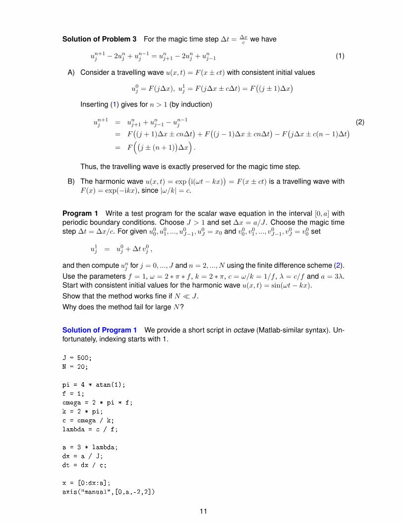
Solution of Problem 3 For the magic time step ∆t = ∆xc we have

un+1j − 2un

j + un−1j = un

j+1 − 2unj + un

j−1 (1)

A) Consider a travelling wave u(x, t) = F (x± ct) with consistent initial values

u0j = F (j∆x), u1

j = F (j∆x± c∆t) = F((j ± 1)∆x

)Inserting (1) gives for n > 1 (by induction)

un+1j = un

j+1 + unj−1 − un−1

j (2)

= F((j + 1)∆x± cn∆t

)+ F

((j − 1)∆x± cn∆t

)− F

(j∆x± c(n− 1)∆t

)= F

((j ± (n + 1)

)∆x)

.

Thus, the travelling wave is exactly preserved for the magic time step.

B) The harmonic wave u(x, t) = exp(i(ωt − kx)

)= F (x ± ct) is a travelling wave with

F (x) = exp(−ikx), since |ω/k| = c.

Program 1 Write a test program for the scalar wave equation in the interval [0, a] withperiodic boundary conditions. Choose J > 1 and set ∆x = a/J . Choose the magic timestep ∆t = ∆x/c. For given u0

0, u01, ..., u

0J−1, u

0J = x0 and v0

0, v01, ..., v

0J−1, v

0J = v0

0 set

u1j = u0

j + ∆t v0j ,

and then compute unj for j = 0, ..., J and n = 2, ..., N using the finite difference scheme (2).

Use the parameters f = 1, ω = 2 ∗ π ∗ f , k = 2 ∗ π, c = ω/k = 1/f , λ = c/f and a = 3λ.Start with consistent initial values for the harmonic wave u(x, t) = sin(ωt− kx).Show that the method works fine if N J .Why does the method fail for large N?

Solution of Program 1 We provide a short script in octave (Matlab-similar syntax). Un-fortunately, indexing starts with 1.

J = 500;

N = 20;

pi = 4 * atan(1);

f = 1;

omega = 2 * pi * f;

k = 2 * pi;

c = omega / k;

lambda = c / f;

a = 3 * lambda;

dx = a / J;

dt = dx / c;

x = [0:dx:a];

axis("manual",[0,a,-2,2])

11

t = 0;

u0 = sin(omega*t-k*x);

v0 = omega * cos(omega*t-k*x);

u = sin(omega*t-k*x);

plot(x,[u;u0]);

t = dt;

u1 = u0 + dt * v0;

u = sin(omega*t-k*x);

plot(x,[u;u1]);

for n=1:N

t = t + dt;

u = sin(omega*t-k*x);

for j=2:J

u2(j) = u1(j+1) + u(j-1) - u0(j);

end;

u2(1) = u1(2) + u(J) - u0(1);

u2(J+1) = u2(1);

plot(x,[u;u2]);

u0 = u1;

u1 = u2;

end;

For N ≥ 70 oscillations start due to rounding errors, which leads to a complete failure forlarger N .

Numerical dispersion

Consider a harmonic wave u(x, t) = exp(i(ωt − kx)

). The equation ∂2

t u = c2∂2xu gives

the dispersion relation ω2 = c2k2 (the dispersion defines a relation of k and ω(k)), and wedefine

phase velocity vp = ω(k)k (= ±c)

group velocity vg = dω(k)dk (= ±c)

Note that we have ddkω2 = 2ω dω

dk = 2c2k, which gives vpvg = c2.In particular we observe, since the harmonic wave has no dispersion, that |vp| = |vg| = c.Now we study phase velocity and group velocity for numerical approximations of the har-monic wave. The ansatz un

j = exp(i(ωn∆t − kj∆x)

)with some k in the finite difference

scheme

un+1j =

(c∆t

∆x

)2(unj+1 − 2un

j + unj−1) + 2un

j − un−1j (3)

yields

exp(i(ω(n + 1)∆t− kj∆x)

)=(

c∆t∆x

)2 exp(i(ωn∆t− kj∆x)

) (exp(−ik∆x)− 2 + exp(ik∆x)

)+2 exp

(i(ωn∆t− kj∆x)

)− exp

(i(ω(n− 1)∆t− kj∆x)

)12

which gives the numerical dispersion relation

cos(ω∆t)− 1 =(c∆t

∆x

)2( cos(k∆x)− 1).

For the magic time step ∆t = ∆xc we obtain k = k. In case of ∆t 6= ∆x

c we obtain numericaldispersion: Consider ∆x = ac∆t and ∆t → 0

=⇒ 1− 12(ω∆t)2 + O(∆t4)− 1 = 1

a2

(1− 1

2

(kac∆t

)2 + O(∆x4)− 1)

=⇒ k = ±ωc + O(∆t2), ω(k)

k= ±c + O(∆t2)

This gives asymptotically vanishing numerical dispersion. From

cos(ω(k)∆t

)− 1 =

(c∆t

∆x

)2( cos(k∆x)− 1)

=⇒d

dk

dω(k)dk

sin(ω(k)∆t

)= c2 ∆t

∆xsin(k∆x)

we obtain for the group velocity

dω(k)dk

=

±c for a = 1 (magic time step)±c + O(∆t2) else

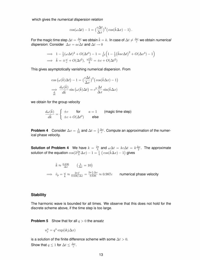
Problem 4 Consider ∆x = λ10 and ∆t = 1

2∆xc . Compute an approximation of the numer-

ical phase velocity.

Solution of Problem 4 We have k = 2πλ and ω∆t = kc∆t = k∆x

2 . The approximatesolution of the equation cos(22π

λ ∆x)− 1 = 14

(cos(k∆x)− 1

)gives

k ≈ 0.636∆x

(λ

∆x = 10)

=⇒ vp = ωk≈ 2πf

0.636/∆x = 2π cλ∆x

0.636 ≈ 0.987c numerical phase velocity

Stability

The harmonic wave is bounded for all times. We observe that this does not hold for thediscrete scheme above, if the time step is too large.

Problem 5 Show that for all q > 0 the ansatz

unj = qn exp(ikj∆x)

is a solution of the finite difference scheme with some ∆t > 0.

Show that q ≤ 1 for ∆t ≤ ∆xc .

13

Solution of Problem 5 The ansatz gives

1(∆t)2

(qn+1 − 2qn + qn−1) exp(ikj∆x)

= c2 1(∆x)2

qn(exp(ik(j + 1)∆x

)− 2 exp(ikj∆x) + exp

(ik(j − 1)∆x

),

=⇒ q2 − 2q + 1 = 2c2(∆t)2

(∆x)2q(cos(k∆x)− 1

)=⇒ q2 − (2 + (∆t)2Λx)q + 1 = 0

for

Λx =2c2

(∆x)2(cos(k∆x)− 1

)∈[ −4c2

(∆x)2, 0],

so that we have

q = p±√

p2 − 1 with p =2 + Λx(∆t)2

2.

This yields |q| ≤ 1 for p2 − 1 ≤ 0, i.e., −1 ≤ p ≤ 1

=⇒ − 4(∆t)2

≤ Λx ≤ 0

=⇒ − 4(∆t)2

≤ − 4c2

(∆x)2⇐⇒ ∆t ≤ ∆x

c .

Consequence The magic time step is the stability bound for the numerical scheme!The interpretation for a point source u0(x) = δ0(x) and v ≡ 0 yields:

CFL-condition (Courant-Friedrichs-Lewy 1929) Stability of a finite difference schemerequires that the domain of dependence of the continuous solution contains the numericaldomain of dependence.

Program 2 Modify Program 1 for ∆t < ∆x/c using the finite difference scheme (3).Show that the method works for J ≈ N .Show that the error at a fixed time T = N∆t is reduced by decreasing ∆t (and thusincreasing N ).

Solution of Program 2

J = 50;

N = 100;

fac = 0.125;

pi = 4 * atan(1);

f = 1;

omega = 2 * pi * f;

k = 2 * pi;

c = omega / k;

lambda = c / f;

14

a = 3 * lambda;

dx = a / J;

dt = fac * dx / c;

q = c*c*dt*dt/(dx*dx);

x = [0:dx:a];

axis("manual",[0,a,-2,2])

t = 0;

u0 = sin(omega*t-k*x);

v0 = omega * cos(omega*t-k*x);

u = sin(omega*t-k*x);

plot(x,[u;u0]);

t = dt;

u1 = u0 + dt * v0;

u = sin(omega*t-k*x);

plot(x,[u;u1]);

for n=1:N

t = t + dt;

for j=2:J

u2(j) = q * (u1(j+1)-2*u1(j)+u(j-1)) + 2*u1(j) - u0(j);

end;

u2(1) = q * (u1(2)-2*u1(1)+u(J)) + 2*u1(1) - u0(1);

u2(J+1) = u2(1);

u = sin(omega*t-k*x);

plot(x,[u;u2]);

u0 = u1;

u1 = u2;

end;

For N = 100 and fac = 0.125 the error gets smaller.

Symplectic schemes

Consider the space of grid functions V∆ = (uj)j∈Z, and let

u = (un) : Z → V∆

n 7→ (unj )

be the discrete time approximation. We define the spatial finite difference operator

(∂2∆xun)j :=

1(∆x)2

(unj+1 − 2un

j + unj−1) L∆ = c2∂2

∆x

15

The scheme above reads un+1−2un+un−1 = (∆t)2 L∆un. We give now another interpre-tation of this scheme, where we split the three term recurrence into two steps. Therefore,we introduce vn+ 1

2 = 1∆t(u

n+1 − un).The Stömer-Verlet scheme (leap-frog method) reads:

vn+1/2 = vn−1/2 + ∆t L∆un (4a)un+1 = un + ∆t vn+1/2 . (4b)

Problem 6 Consider periodic solutions with u(0) = u(a) and v(0) = v(a). Show that theHamiltonian

H(v, u) =∫ a

0

(12|v|2 +

12c2|∂xu|2

)dx

remains constant along a periodic solution of the wave equation.

Solution of Problem 6 Inserting v = ∂tu and integration by parts gives

∂tH(v, u) =∫ a

0l(v∂tv + c2∂xu∂t∂xu

)dx

=∫ a

0l(∂tu∂2

t u− c2∂tu∂2xu)dx = 0 .

Program 3 Modify Program 2 for the leap frog scheme (4), starting with

v1/2 = v0 +12∆t L∆u0 .

Show that the method works for J N , if ∆t < ∆x/c

Show the effect of numerical dispersion.

Solution of Program 3

J = 50;

N = 400;

fac = 0.8;

pi = 4 * atan(1);

f = 1;

omega = 2 * pi * f;

k = 2 * pi;

c = omega / k;

lambda = c / f;

a = 3 * lambda;

dx = a / J;

dt = fac * dx / c;

q = c*c/(dx*dx);

x = [0:dx:a];

16

axis("manual",[0,a,-2,2])

t = 0;

u0 = sin(omega*t-k*x);

v0 = omega * cos(omega*t-k*x);

u_n = u0;

u = sin(omega*t-k*x);

plot(x,[u;u_n]);

t = 0.5 * dt;

for j=2:J

v_n(j) = v0(j) + 0.5 * dt * q * (u_n(j+1)-2*u_n(j)+u_n(j-1));

end;

v_n(1) = v0(1) + 0.5 * dt * q * (u_n(2)-2*u_n(1)+u_n(J));

v_n(J+1) = v_n(1);

for n=1:N

t = t + 0.5*dt;

u = sin(omega*t-k*x);

u_n = u_n + dt * v_n;

plot(x,[u;u_n]);

t = t + 0.5*dt;

for j=2:J

v_n(j) = v_n(j) + dt * q * (u_n(j+1)-2*u_n(j)+u_n(j-1));

end;

v_n(1) = v_n(1) + dt * q * (u_n(2)-2*u_n(1)+u_n(J));

v_n(J+1) = v_n(1);

end;

The Yee scheme for the wave equation in 1D

Another possibility for the construction of stable schemes are obtained by a reformulationas a first order system. Consider

∂t

(u

w

)=

(0 c

c 0

)∂x

(u

w

),

i.e., ∂tu = c∂xw and ∂tw = c∂xu. This gives

∂2t u = c∂x∂tw = c2∂2

xu .

Now we consider a finite interval [0, a] and homogeneous boundary conditions

u(0, t) = u(a, t) = 0, t > 0

and initial conditions

u(x, 0) = u0(x) , w(x, 0) = w0(x) , x ∈ (0, a) .

17

This system has a first integral I(u, w) =12

∫ a

0(|u|2 + |w|2)dx, since the homogeneous

boundary conditions and integration by parts yield

∂tI(u, w) =∫ a

0(u∂tu + w∂tw) dx

=∫ a

0(c∂xwu + c∂xu w) = 0 .

A semi-discrete scheme

First we discuss a scheme which is discrete in space but continuous in time:

∂twj+1/2 =c

∆x(uj+1 − uj)

∂tuj =c

∆x(wj+1/2 − wj−1/2)

Here, w is approximated at xj+1/2 = (j + 1/2)∆x and u is approximated at xj = j∆x.

Problem 7 Consider in [0, a] with ∆x = a/J and u0(t) ≡ uJ(t) ≡ 0. Show that thesemi-discrete scheme preserves the quantity

I∆(u, w) =J∑

j=1

∆x(|uj |2 + |wj−1/2|2) .

Solution of Problem 7 Summation by parts and periodic extension gives

d

dtI∆(u, w) =

J∑j=1

∆x

∆x

(ujc(wj+1/2 − wj−1/2) + wj−1/2c(uj − uj−1

)= 0 .

A staggered scheme in space and time

A fully discrete scheme uses in addition the staggered time discretization (cf. the leap frogscheme)

wn+1/2j+1/2 = w

n−1/2j+1/2 + c

∆t

∆x

(un

j+1 − unj

)(5a)

un+1j = un

j + c∆t

∆x

(w

n+1/2j+1/2 − w

n+1/2j−1/2

). (5b)

Program 4 Modify Program 3 for the Yee scheme (5) and for homogeneous boundaryconditions, starting with

u0j = 1, j = 1, ..., J − 1

w1/2j−1/2 = 0, j = 1, ..., J − 1

and u00 = u0

J = 0. Compare the numerical solution with the analytical solution in Prob-lem 1.

18

Solution of Program 4

J = 100;

N = 500;

fac = 0.5;

pi = 4 * atan(1);

f = 1;

omega = 2 * pi * f;

k = 2 * pi;

c = omega / k;

lambda = c / f;

a = 3 * lambda;

dx = a / J;

dt = fac * dx / c;

q = c * dt / dx;

x = [0:dx:a];

axis("manual",[0,a,-2,2])

t = 0;

u = x;

w = u;

for j=1:J

u(j) = 1;

w(j) = 0;

end;

u(1) = 0;

u(J+1) = 0;

plot(x,u);

for n=1:N

t = t + dt;

for j=2:J

u(j) = u(j) + q * (w(j) - w(j-1));

end;

for j=1:J

w(j) = w(j) + q * (u(j+1) - u(j));

end;

plot(x,u);

end;

Now, the reader should be prepared to read [5] for a full numerical analysis of this problem.

19

2 The FDTD method for Maxwell’s equations

Before we start to derive a numerical scheme, we summarize some analytical results.Let Ω ⊂ R3 be a domain, ε, µ ∈ L∞(Ω, R3,3) with

ξT ε(x)ξ ≥ ε0|ξ|2 , ξT µ(x)ξ ≥ µ0|ξ|2 , ∀ ξ ∈ R3 , ε0, µ0 > 0 . (6)

Consider the Maxwell system

ε ∂tE −∇×H = 0µ ∂tH +∇× E = 0

with σ ≡ 0 (no conductivity) subject to boundary and initial conditions

E(x, t)× n(x) = 0 , (x ∈ ∂Ω) , E(x, 0) = E0(x), H(x, 0) = H0(x) (x ∈ Ω) .

Define U(t) =(

E(t)H(t)

)∈ X := L2(Ω, C3)× L2(Ω, C3), set U0 =

(E0

H0

). We use the inner

product 〈U, V 〉X =∫

ΩU ·M V dx with M =

(ε 00 µ

)∈ L∞(Ω, R6,6).

Lemma 5. The operator A = iM−1

(0 − curl

curl 0

)is self-adjoint in X with domain

D(A) = H0(curl, Ω)×H(curl, Ω) ,

where

H(curl, Ω) = u ∈ L2(Ω, C3) : curl u ∈ L2(Ω, C3) ,

H0(curl, Ω) = u ∈ H(curl, Ω) : u× n = 0 on ∂Ω .

Proof. For vectors a, b, c ∈ C3 we have a · (b × c) = (a × b) · c = (c × a) · b, for vectorfields u,v : Ω → C3 we have ∇ · (u × v) = v · (∇ × u) − u · (∇ × v). Thus, the Gaußtheorem gives∫

Ωv ·(∇×u)dx−

∫Ω

u ·(∇×v)dx =∫

Ω∇·(u×v)dx =

∫∂Ω

(u×v) ·da =∫

∂Ωu ·(v×n)da

which implies for u ∈ H(curl, Ω) and v ∈ H0(curl, Ω)∫Ω

v · curlu dx =∫

Ωu · curlv dx .

Thus, we have

〈A U, V 〉X = i∫

Ω

((− curlU2) · V1 + curlU1 · V2

)dx

= −i∫

Ω(U2 · curl V1 − U1 · curl V2)dx = 〈U,A V 〉X ,

i.e., A is symmetric. Thus, we have A ⊂ A∗, where A∗ : D(A∗) → X is defined onD(A∗) = U ∈ X : there exists V ∈ X with 〈V,W 〉X = 〈U,AW 〉 ∀W ∈ D(A); then set

20

A∗U = V (this defines V uniquely, since D(A) is dense in X).We finally have to prove D(A∗) = D(A). For U ∈ D(A∗) we consider

W =(

εE0

)∈ D(A) =⇒

∫Ω

V1 · εEdx = −i∫

ΩU2 · curl E dx .

Thus, the weak derivative curlU2 is in L2 and εV1 = −i curlU2. Analogously, we getµV2 = i curl U1 and U × n = 0 on ∂Ω.

The Maxwell Cauchy problem is of the form

U + i A U = 0 U(0) = U0 .

It has a unique solution, and since A is self-adjoint, it has the representation

U(t) = exp(−iA t)U0 =∫ ∞

−∞exp(−iλ t)dP (λ)U0 .

The energy E(t) := ‖U(t)‖2X ≡ E(0) is conserved, since we have

∂tE(t) = 〈∂tU,U〉+ 〈U, ∂tU〉 = −i〈AU,U〉+ i〈U,AU〉 = 0 .

Problem 8 Prove that the kernel N(A) = U ∈ M : AU = 0 is infinite-dimensional.

Solution of Problem 8 Choose open sets ωn ⊂ Ω with |ωn| < 1n (n ∈ N) and such that

ωn ∩ ωm = ∅ for n 6= m. Choose φn ∈ C∞0 (ωn) such that Un =

(∇φn

0

)is normalized with

‖Un‖ = 1. This gives curl∇φn = 0 and thus AUn = 0. Since (Un)n∈N is orthonormal in X,we have infinitely many linear independent kernel vectors.

The semi-discrete scheme

Now we consider the Finite-Difference-Time-Domain method (introduced 1966 by K.S.Yee) for the system

ε ∂tE −∇×H = J

µ ∂tH +∇× E = 0 .

For ∆x > 0 define the grid Z∆ = ∆xZ3. Set xj = j ∆x.We consider Maxwell’s equations on the domain Ω = (0, J1∆x) × (0, J2∆x) × (0, J3∆x)with absorbing boundary conditions E × n = 0 on ∂Ω. The grid points Z∆ ∩ Ω are thecorners of a uniform hexahedral mesh with J1J2J3 cells.We assume that the solution

(E(t),H(t)

)=(E1(t), E2(t), E3(t),H1(t),H2(t),H3(t)

)of the

continuous problem is sufficiently smooth. We compute approximations E = (E1, E2, E3)on edge midpoints and H = (H1,H2,H3) on face midpoints of H, i.e., approximations

Ei+1/2, j, k(t) of E1(xi+1/2, xj , xk, t)Ei, j+1/2, k(t) of E2(xi, xj+1/2, xk, t)Ei, j, k+1/2(t) of E3(xi, xj , xk+1/2, t)Hi, j+1/2, k+1/2(t) of H1(xi, xj+1/2, xk+1/2, t)Hi+1/2, j, k+1/2(t) of H2(xi+1/2, xj , xk+1/2, t)Hi+1/2, j+1/2, k(t) of H3(xi+1/2, xj+1/2, xk, t) ,

21

by evaluating Maxwell’s equations in integral form with midpoint quadrature formulae.

The application of Faraday’s law ∂t

∫A

µH · da = −∫

∂AE · dl with the face

A = Ai,j+1/2,k+1/2 := xi × [xj , xj+1]× [xk, xk+1]

together with midpoint quadrature gives

(∆x)2µi,j+1/2,k+1/2∂tHi,j+1/2,k+1/2 = ∆x(−Ei,j+1,k+1/2+Ei,j,k+1/2−Ei,j+1/2,k+Ei,j+1/2,k+1) .

This motivates the definition of the finite difference approximation of the curl component indirection of the normal ni,j+1/2,k+1/2 of Ai,j+1/2,k+1/2 at the face midpoint (xi, xj+1/2, xk+1/2)by

(∆x)2 curli,j+1/2,k+1/2 E = ∆x(Ei,j+1,k+1/2 − Ei,j,k+1/2 + Ei,j+1/2,k − Ei,j+1/2,k+1) .

Thus, we can rewrite the finite difference equation as

µi,j+1/2,k+1/2∂tHi,j+1/2,k+1/2 = − curli,j+1/2,k+1/2 E .

In the same way, the application to the face Ai+1/2,j,k+1/2 = [xi, xi+1] × xj × [xk, xk+1]gives

(∆x)2µi+1/2,j,k+1/2∂tHi+1/2,j,k+1/2 = ∆x(−Ei,j,k+1/2+Ei+1,j,k+1/2−Ei+1/2,j,k+1+Ei+1/2,j,k) ,

which rewrites (by introducing a discrete curl component) as

µi+1/2,j,k+1/2∂tHi+1/2,j,k+1/2 = − curli+1/2,j,k+1/2 E .

Analogously, we obtain

(∆t)2µi+1/2,j+1/2,k∂tHi+1/2,j+1/2,k = ∆t(−Ei+1,j+1/2,k+Ei,j+1/2,k−Ei+1/2,j,k+Ei+1/2,j+1,k) ,

i. e.,µi+1/2,j+1/2,k∂tHi+1/2,j+1/2,k = − curli+1/2,j+1/2,k E .

Now, the application to Ampère’s law∫

A(ε∂tE − J) · da =

∫∂A

H · dl to the surface

Ai+1/2,j,k = xi+1/2 × [xj+1/2, xj+1/2]× [xk−1/2, xk+1/2]

(orthogonal to the edge midpoint (xi+1/2, xj , xk)) gives

(∆x)2(εi+1/2,j,k∂tEi+1/2,j,k−Ji+1/2,j,k) = ∆x(Hi+1/2,j+1/2,k−Hi+1/2,j−1/2,k+Hi+1/2,j,k−1/2−Hi+1/2,j,k+1/2) .

As above, we write

εi+1/2,j,k∂tEi+1/2,j,k − Ji+1/2,j,k = curli+1/2,j,k H ,

and integration along Ai,j+1/2,k and Ai+1/2,j,k+1/2 gives

εi,j+1/2,k∂tEi,j+1/2,k − Ji,j+1/2,k = curli,j+1/2,k H ,

εi,j+1/2,k∂tEi,j+1/2,k − Ji,j+1/2,k = curli,j+1/2,k H .

We set Eα,β,γ = 0 for all boundary points (xα, xβ, xγ) ∈ ∂Ω.

22

Discrete compatibility

We have∫

Vdiv J dx =

∫∂V

J · da. Evaluating this for the volume

V = (xi−1/2, xi+1/2)× (xj−1/2, xj+1/2)× (xk−1/2, xk+1/2)

motivates the following definition for the discrete divergence at (xi, xj , xk) by

(∆x)3 divi,j,k J = (∆x)2(Ji+1/2,j,k−Ji−1/2,j,k+Ji,j+1/2,k−Ji,j−1/2,k+Ji,j,k+1/2−Ji,j,k−1/2) .

It can be shown that for compatible data divi,j,k J = 0 and compatible initial valuesdivi,j,k εE(0) = 0 and divi+1/2,j+1/2,k+1/2 µH(0) = 0 we have

divi,j,k εE(t) = 0, divi+1/2,j+1/2,k+1/2 µH(t) = 0

for all t > 0.

Convergence

It can be shown (for suitable norms) that we have

‖E(t)−E(t)‖E + ‖H(t)−H(t)‖H ≤ (C0 + t C1)∆x

for t ∈ [0, T ] and C0, C1 depending on T (see [8]).

Problem 9 Construct the corresponding fully discrete scheme.

Solution of Problem 9 Again, together with leap frog we get the scheme

µi,j+1/2,k+1/2Hn+1/2i,j+1/2,k+1/2 = µi,j+1/2,k+1/2H

n−1/2i,j+1/2,k+1/2 −∆t curli,j+1/2,k+1/2 En ,

µi+1/2,j,k+1/2Hn+1/2i+1/2,j,k+1/2 = µi+1/2,j,k+1/2H

n−1/2i+1/2,j,k+1/2 −∆t curli+1/2,j,k+1/2 En ,

µi+1/2,j+1/2,kHn+1/2i+1/2,j+1/2,k = µi+1/2,j+1/2,kH

n−1/2i+1/2,j+1/2,k −∆t curli+1/2,j+1/2,k En ,

εi+1/2,j,kEn+1i+1/2,j,k = εi+1/2,j,kE

ni+1/2,j,k + J

n+1/2i+1/2,j,k + ∆t curli+1/2,j,k Hn+1/2 ,

εi,j+1/2,kEn+1i,j+1/2,k = εi,j+1/2,kE

ni,j+1/2,k + J

n+1/2i,j+1/2,k + ∆t curli,j+1/2,k Hn+1/2 ,

εi,j+1/2,kEn+1i,j+1/2,k = εi,j+1/2,kE

ni,j+1/2,k + J

n+1/2i,j+1/2,k + ∆t curli,j+1/2,k Hn+1/2 .

Remark

The error is (slowly) growing in time, so that the application to photonics (where we havesmall wave lengths) is very restrictive. On the other hand, it is extremely difficult to con-struct schemes with better properties, so that the spectral analysis of the Maxwell operatoris the only safe method for a qualitative numerical analysis of photonic waves.

23

3 Time-harmonic solutions and eigenfrequencies

We insert into the Maxwell system

ε∂tE − curlH = 0 µ∂tH + curlE = 0div(εE) = 0 div(µH) = 0

a time-harmonic ansatz for a monochromatic wave with frequency ω:

E(x, t) = E(x) exp(iωt) , H(x, t) = H(x) exp(iωt) .

This gives

∂tE = iωE , ∂tH = iωH , curlE = exp(iωt) curl E ,

and from iω εE − curlH = 0, iω µH + curlE = 0 we obtain

iω εE − curlH = 0 iω µH + curlE = 0div(εH) = 0 div(µH) = 0 .

(7)

Now, curl ε−1 curlH = iω curlE = iω(−iω)µH = ω2µH yields a decoupled system

curl ε−1 curlH = ω2µH div(µH) = 0curlµ−1 curlE = ω2εE div(εE) = 0

These are eigenvalue problems with eigenvalue λ = ω2. Thus, it suffices to find Maxwelleigenfunctions and corresponding eigenvalues in order to construct time-harmonic solu-tions of the full Maxwell system.

The Maxwell eigenvalue problem

Let Ω ⊂ R3 be a Lipschitz domain, and consider the spaces

H0(curl, Ω) = u ∈ L2(Ω, C3) : curl u ∈ L2(Ω, C3), u× n = 0 on ∂ΩV = u ∈ H0(curl, Ω) :

∫µu∇pdx = 0 ∀ p ∈ C∞

0 (Ω)H1

0 = p ∈ L2(Ω) : ∇p ∈ L2(Ω, C3) p = 0 on ∂Ω

and assume (6) for the parameters ε, µ.Then, the eigenvalue problem in weak form

H ∈ V :∫

ΩcurlH · ε−1 · curlϕdx = λ

∫Ω

µHϕ dx

has the null-space ∇H10 (Ω) and a discrete spectrum σ = 0, λ1, λ2 . . . with eigenvalues

0 < λ1 ≤ λ2 ≤ . . . .

Problem 9 Consider a 3-d layered structure in x1-direction, i.e., all quantities are inde-pendent of the variables x2 and x3, i.e., ε = ε(x1) ∈ R, µ = µ(x1) ∈ R. Show that we havein this case for the components of the magnetic field H1 ≡ 0 and −∂1ε

−1∂1Hj = ω2µHj

(j = 2, 3).

24

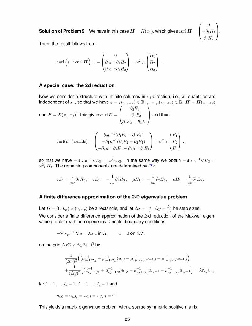
Solution of Problem 9 We have in this case H = H(x1), which gives curlH =

0−∂1H3

∂1H2

.

Then, the result follows from

curl(ε−1 curlH

)= −

0∂1ε

−1∂1H2

∂1ε−1∂1H3

= ω2 µ

H1

H2

H3

.

A special case: the 2d reduction

Now we consider a structure with infinite columns in x3-direction, i.e., all quantities areindependent of x3, so that we have ε = ε(x1, x2) ∈ R, µ = µ(x1, x2) ∈ R, H = H(x1, x2)

and E = E(x1, x2). This gives curlE =

∂2E3

−∂1E3

∂1E2 − ∂2E1

and thus

curl(µ−1 curlE) =

∂2µ−1(∂1E2 − ∂2E1)

−∂1µ−1(∂1E2 − ∂2E1)

−∂2µ−1∂2E3 − ∂1µ

−1∂1E3

= ω2 ε

E1

E2

E3

.

so that we have −div µ−1∇E3 = ω2εE3. In the same way we obtain −div ε−1∇H3 =ω2µH3. The remaining components are determined by (7):

εE1 =1iω

∂2H3 , εE2 = − 1iω

∂1H3 , µH1 = − 1iω

∂2E3 , µH2 =1iω

∂1E3 .

A finite difference approximation of the 2-D eigenvalue problem

Let Ω = (0, Lx)× (0, Ly) be a rectangle, and let ∆x = LxJx

, ∆y = Ly

Jybe step sizes.

We consider a finite difference approximation of the 2-d reduction of the Maxwell eigen-value problem with homogeneous Dirichlet boundary conditions

−∇ · µ−1 ∇u = λ ε u in Ω , u = 0 on ∂Ω .

on the grid ∆xZ×∆yZ ∩ Ω by

1(∆x)2

((µ−1

i+1/2,j + µ−1i−1/2,j)ui,j − µ−1

i+1/2,jui+1,j − µ−1i−1/2,jui−1,j

)+

1(∆y)2

((µ−1

i,j+1/2 + µ−1i,j−1/2)ui,j − µ−1

i,j+1/2ui,j+1 − µ−1i,j−1/2ui,j−1

)= λεi,jui,j

for i = 1, ..., Jx − 1, j = 1, ..., Jy − 1 and

ui,0 = ui,Jy = u0,j = uJx,j = 0 .

This yields a matrix eigenvalue problem with a sparse symmetric positive matrix.

25

Program 5 Compute the eigenvalues of the 2-d reduced problem in the unit squareΩ = (0, 1)2 with Jx = Jy = J for µ ≡ 1 and

ε(x, y) =

7 0.25 ≤ x, y ≤ 0.751 else.

Study the convergence properties of the smallest eigenvalue in dependence of J .

Solution of Program 5

J = 40;

dx = 1 / J;

N = (J-1)*(J-1);

A = zeros(N,N);

M = ones(N,1);

for i=1:N

A(i,i) = 4;

end;

for i=1:J-1

for j=1:J-2

k = (i-1)*(J-1) + j;

A(k,k+1) = -1;

A(k+1,k) = -1;

k = (j-1)*(J-1) + i;

A(k,k+J-1) = -1;

A(k+J-1,k) = -1;

end;

end;

for i=1:J-1

x = i * dx;

if (x >= 0.25)

if (x <= 0.75)

for j=1:J-1

y = j * dx;

if (y >= 0.25)

if (y <= 0.75)

k = (i-1)*(J-1) + j;

M(k) = 1 / sqrt(7);

end;

end;

end;

end;

end;

end;

for i=1:N

for j=1:N

A(i,j) = A(i,j) * M(i) * M(j);

26

end;

end;

ev = eig(A);

for i=1:N

ev(i) = ev(i) / (dx*dx);

end;

This yields

J = 5 J = 10 J = 20 J = 40 J = 80 J=100 J = 120

λ1 4.0593 3.6638 3.4684 3.6069 3.6796 3.6945 3.7044λ2 = λ3 11.627 11.175 10.408 11.177 11.573 11.653 11.706

λ4 19.445 20.321 18.937 20.753 21.684 21.871 21.996

For more precise results, more efficient methods are required.

27