Numerische Mathematik - hu-berlin.decc/cc_homepage/download/1996-BU_CC_SE...Numer. Math. (1996) 75: 153–174 Numerische Mathematik c Springer-Verlag 1996 Electronic Edition Symmetric

Numer. Math. (1996) 75: 153–174 NumerischeMathematikc© Springer-Verlag 1996

Electronic EditionSymmetric coupling of boundary elementsand Raviart–Thomas-type mixed finite elementsin elastostatics

Ulrich Brink 1, Carsten Carstensen2, Erwin Stein1

1 Institut fur Baumechanik und Numerische Mechanik, Universitat Hannover, D-30167 Hannover,Germany2 Mathematisches Seminar II, Christian-Albrechts-Universitat zu Kiel, D-24098 Kiel, Germany

Received February 21, 1995 / Revised version received December 21, 1995

Dedicated to Professor G. C. Hsiao on occasion of his 60th birthday.

Summary. Both mixed finite element methods and boundary integral methodsare important tools in computational mechanics according to a good stress ap-proximation. Recently, even low order mixed methods of Raviart–Thomas-typebecame available for problems in elasticity. Since either methods are robust forcritical Poisson ratios, it appears natural to couple the two methods as proposedin this paper. The symmetric coupling changes the elliptic part of the bilinearform only. Hence the convergence analysis of mixed finite element methods isapplicable to the coupled problem as well. Specifically, we couple boundary el-ements with a family of mixed elements analyzed by Stenberg. The locking-freeimplementation is performed via Lagrange multipliers, numerical examples areincluded.

Mathematics Subject Classification (1991):65N30, 65R20

1. Introduction

In the classical finite element approach, the displacements are the unknowns whilethe stresses are computed afterwards in lower accuracy. In many applications,the stresses rather than the displacements are of primary interest. In the boundaryelement method (BEM), displacements and stresses in the interior of the domainare approximated with the same order.

Regarding finite elements, the approximation of the stresses can be improvedby mixed methods. Here we consider Raviart–Thomas-type finite elements due toStenberg [11], which are an improvement of Arnold–Brezzi–Douglas’s PEERSelement (plane elasticity element with reduced symmetry) [1]. The unknowns arethree independent fields, namely the stress tensor, which is not a priori assumedto be symmetric, the rotation, which acts as a Lagrange multiplier to enforcethe symmetry of the stress tensor in a weak form, and the displacement vector.

Numerische Mathematik Electronic Editionpage 153 of Numer. Math. (1996) 75: 153–174

154 U. Brink et al.

The analysis is based on the theory of mixed methods but refined by usingmesh-dependent norms (Pitkaranta and Stenberg [9], [10]), by stability proofs onpatches of elements and by weakening of the symmetry condition.

Another advantage of these elements is the capability of modeling nearlyincompressible elasticity; more precisely, the relative error is independent ofPoisson’s ratioν: there is no locking.

In many applications, for example, if nonlinearities in a bounded domainΩF are present as well as homogeneous, isotropic linear elastic material in anunbounded, e.g., exterior, domainΩB, one might combine the finite elementmethod (inΩF) with the boundary integral method (acting on∂ΩB but treating theproblem inΩB). The symmetric coupling with boundary elements was proposedand analyzed by Costabel in [6] where the displacements inside the FEM domainare sought in the Sobolev spaceH 1(ΩF); traces on the interface are inserted intothe boundary integral equations, while the equilibrium of tractions across theinterface is satisfied in a weak sense only.

In contrast, in the mixed FEM under consideration here, the stressesσ arerequired to satisfyσ ∈ L2(ΩF) and divσ ∈ L2(ΩF), while the displacements aresought inL2(ΩF) only. Hence, the discrete tractions across interelement sides arecontinuous and, consequently, our coupled scheme is designed to yield continuoustractions across the interface between FEM and BEM while continuity of thedisplacements across the interelement sides and the interface is satisfied in aweak sense.

The construction of finite element spaces with continuous interelement trac-tions may be cumbersome and hence is enforced by using Lagrange multipliers.Then all unknowns, except the Lagrange multipliers, are discontinuous acrossthe interelement sides and can be eliminated on each element before assemblingthe global linear system. We extended this scheme to the coupled system.

A similar coupling is possible with other mixed finite element methods thanthose considered in this paper. The weakening of the symmetry of the stresstensor is a particular way to construct stable finite element spaces, but is by nomeans necessary for the coupling.

The paper is organized as follows: A model problem (as depicted in Fig. 1)is described in its strong form in Sect. 2 and rewritten in a weak form. We proveexistence and uniqueness of solutions and a norm estimate by using Brezzi’stheory of mixed problems. The discretization is described in Sect. 3 where westate convergence estimates under some hypotheses on the mixed finite elementmethods. Proofs are given in Sect. 4 while in Sect. 5 Stenberg’s locking-free fam-ily of methods is discussed. We describe the implementation by using Lagrangemultipliers in Sect. 6 and give some numerical examples in Sect. 7.

2. The coupled problem

Let Ω be a bounded polygonal (resp. polyhedral) domain inRd, d = 2 (resp.

d = 3) with boundary∂Ω = Γu ∪ Γt with disjoint Γu andΓt , either having apositive surface measure.


Symmetric coupling of BEM and mixed FEM 155

Γu ΩF

FEM

Γt

-n

n

ΩB

BEM

Γ

Fig. 1. Notation

Throughout this paper, we consider the linear elasticity problem

divσ = −f in Ωσ = Cε(u) in Ωu = 0 onΓu

σn = 0 onΓt .

(2.1)

The displacement field is denoted byu, the related (linear Green) strain tensoris ε(u) = 1

2( gradu + ( gradu)T). The elasticity tensorC describes the stress–strain relationship; in the simplest case we haveσ = Cε = λ tr εI + 2µε whereλ whereµ are the Lame coefficients andI denotes the identity matrix. (In thetwo-dimensional case, this is the constitutive equation of plane strain).

As depicted in Fig. 1, the domainΩ is partitioned intoΩ = ΩF ∪ Γ ∪ ΩB;the outward unit normal ofΩF is denoted byn.

OnΩF a mixed finite element method based on the Hellinger–Reissner prin-ciple is applied. This means the displacementu : ΩF → R

d and the stressσ : ΩF → R

d×d are independent unknowns. Furthermore, the stress tensorσis not a priori assumed to be symmetric. Symmetry will be enforced in a weakform by a Lagrange multiplier technique. To obtain a variational formulation, wechoose test functionsτ : ΩF → R

d×d satisfyingτn = 0 on Γt , and gain from(2.1)b ∫

ΩF

τ : C−1σ dΩ −∫ΩF

τ : ε(u) dΩ = 0

so that integration by parts gives∫ΩF

τ : C−1σ dΩ +∫ΩF

div τ · u dΩ +∫ΩF

τ : γ dΩ =∫Γ

τn · u ds


156 U. Brink et al.

where the rotationγ := 12( gradu − ( gradu)T) is a new variable for the skew-

symmetric part of the displacement gradient,

γ ∈ W := η ∈ L2(ΩF)d×d : η + ηT = 0.The stresses and displacements are sought in

H := τ ∈ L2(ΩF)d×d : div τ ∈ L2(ΩF)d, τn = 0 onΓt,L := L2(ΩF)d.

H is a Hilbert space when endowed with the norm

‖τ‖div := (‖τ‖20,ΩF

+ ‖ div τ‖20,ΩF

)1/2.

In summary, the variational form of the problem inΩF reads: Given a body loadf and a displacementϕ on Γ , find (u, σ, γ) ∈ L ×H ×W satisfying∫

ΩFτ : C−1σ dΩ +

∫ΩF

div τ · u dΩ+∫ΩFτ : γ dΩ =

∫Γτn ·ϕ ds ∀τ ∈ H∫

ΩFdivσ · v dΩ = − ∫

ΩFf · v dΩ ∀v ∈ L∫

ΩFσ : η dΩ = 0 ∀η ∈ W .

(2.2)

The identity (2.2)a is derived above, (2.2)b is a weak form of (2.1)a, and (2.2)cis a weak form of the symmetry ofσ.

We assume that the body loadf ∈ L2(Ω)d vanishes onΩB for simplicity andthat the Lame coefficients are constant onΩB. Then, at any pointx ∈ ΩB, thedisplacement field can be represented by the Betti formula

u(x) = −∫Γ

G(x, y) Tyu(y) dsy +∫Γ

(TyG(x, y)

)Tu(y) dsy .

Here Tyu(y) = Cε(u(y)) n(y) is the traction corresponding tou at a pointy ∈Γ , and TyG(x, y) are the columnwise tractions ofG(x, y) at y. G(x, y) is thefundamental solution and equals

λ+3µ4πµ(λ+2µ)

log 1

|x−y| I + λ+µλ+3µ

(x−y)(x−y)T

|x−y|2

if d = 2,

λ+3µ8πµ(λ+2µ)

1

|x−y| I + λ+µλ+3µ

(x−y)(x−y)T

|x−y|3

if d = 3.

Letting x → Γ we obtain with the classical jump relations the boundary integralequation

12u = −Vt + Ku(2.3)

with t(y) = Tyu(y) and the integral operators

(Vt)(x) =∫Γ

G(x, y) t(y) dsy, x ∈ Γ,

(Ku)(x) =∫Γ

(TyG(x, y)

)Tu(y) dsy, x ∈ Γ .



Applying the traction operatorTx we get another boundary integral equation

12t = −K ′t −Wu(2.4)

where

(K ′t)(x) =∫Γ

TxG(x, y) t(y) dsy, x ∈ Γ ,

(Wu)(x) = −Tx

∫Γ

(TyG(x, y)

)Tu(y) dsy, x ∈ Γ .

The symmetric coupling of (2.2) with the integral equations (2.3) and (2.4) isperformed as follows: Introduce a new variableϕ := u|Γ belonging to the tracespace

H 1/2 := H 1/2(Γ)d := u|Γ : u ∈ H 1(Ω)d,and use continuity of the tractions onΓ , i.e., t = σn. Then, (2.3) reads

ϕ = −V (σn) + (12I + K )ϕ

and this is inserted in the right-hand side of (2.2)a while (2.4) reads

Wϕ + (12I + K ′)(σn) = 0

and this is added in a weak form to (2.2). (This coupling is in a sense ‘dual’ to themore classical approach, see e.g. [4, 6, 7], where a new variable is introducedfor σn on the interface while foru|Γ continuity is used.) The resulting weakformulation is rewritten in a saddle point structure: Find (σ, ϕ, u, γ) ∈ H ×H 1/2 ×L ×W such that

a(σ, ϕ; τ, ψ) + b(τ ; u, γ) = 0b(σ; v, η) = − ∫

ΩFf · v dΩ

(2.5)

for all (τ, ψ, v, η) ∈ H × H 1/2 ×L ×W . Here,

a(σ, ϕ; τ, ψ) :=∫ΩF

τ : C−1σ dΩ

+ 〈τn , V (σn)〉 − ⟨τn , ( 12I + K )ϕ

⟩− 〈ψ , Wϕ〉 − ⟨ψ , ( 1

2I + K ′)(σn)⟩

b(σ; v, η) :=∫ΩF

divσ · v dΩ +∫ΩF

σ : η dΩ.

Throughout this paper,〈ϕ , ψ〉 denotes the extension of theL2-scalar product∫Γϕ ·ψ ds to the duality inH−1/2 × H 1/2; H s := H s(Γ )d.


158 U. Brink et al.

Remark 2.1.It is known that the mappingsV : H−1/2 → H 1/2, K : H 1/2 →H 1/2, K ′ : H−1/2 → H−1/2, W : H 1/2 → H−1/2 are well defined, linear andcontinuous (cf., e.g., [5]).V and W are symmetric;K ′ is dual to K and Wis positive semi-definite and kerW = kerε|Γ , i.e., the kernel ofW consists ofthe (linearized) rigid body motions.W is positive definite on (H 1/2/ kerε)2. Ford = 3, V is positive definite. Ford = 2, V is positive definite when restricted toH−1/2

0 where

H s0 := w ∈ H s :

∫Γ

w ds = 0 ≡ H s/Rd.

We refer to [7] for proofs in cased = 3 and mention that the proofs work verbatimin cased = 2 (provided the radiation condition gives a sufficiently strong decaywhich is guaranteed owing to the restriction onH−1/2

0 ).

Remark 2.2.We note thatσn is defined inH−1/2 via Green’s formula even ifσ ∈ H as follows. Givenv ∈ H 1/2 extend it to somev ∈ H 1(ΩF)d withv|Γu = 0. Then, let

〈v , σn〉 :=∫ΩF

σ : gradv dΩ +∫ΩF

v · divσ dΩ.

The right-hand side is well defined and depends linearly and continuously onvandσ. Furthermore,

‖σn‖−1/2,Γ ≤ C ‖σ‖div .(2.6)

In view of the remarks,a is a symmetric and continuous bilinear form on(H × H 1/2)2, andb is continuous onH × (L ×W ).

Theorem 2.1. For every f ∈ L2(ΩF)d the saddle point problem(2.5)has a uniquesolution satisfying

‖σ‖0,ΩF + ‖ divσ‖0,ΩF + ‖ϕ‖1/2,Γ + ‖u‖0,ΩF + ‖γ‖0,ΩF ≤ C ‖f ‖0,ΩF(2.7)

with a positive constant C which is independent of f .

Proof. We apply the theory of saddle point problems, cf., e.g., [3, Sect. II.1]. Itis sufficient to verify surjectivity ofb and the inf–sup condition ona. As it iswell known, the bilinear formb has the following surjectivity property: For all(v, η) ∈ L ×W there is someτ ∈ H satisfying

div τ = v and asτ := 12(τ − τT) = η.(2.8)

Therefore, it remains to prove that, for a constantα > 0,

inf(σ,ϕ)

sup(τ,ψ)

a(σ, ϕ; τ, ψ)( ‖σ‖0,ΩF + ‖ϕ‖1/2,Γ )( ‖τ‖0,ΩF + ‖ψ‖1/2,Γ )

≥ α(2.9)

where in inf(σ,ϕ) and sup(τ,ψ) the nonzero arguments run through kerB,

kerB := τ ∈ H : div τ = 0 and asτ = 0 × H 1/2 .



We will prove (2.9) in two steps partly arguing as in [4]: Given (σ, ϕ) ∈ kerBlet ϕ = ϕ0 + r0 whereϕ0 ∈ H 1/2/ kerε andr0 ∈ kerε, kerε the (linearized) rigidbody motions. Lettc ∈ Rd be defined by∫

Γ

(σn − tc) ds = 0.

Then, letσc := Cε(uc) whereuc ∈ H 1(ΩF)d is the solution of divσc = 0 onΩF

while σcn = tc on Γ , σcn = 0 onΓt anduc = 0 onΓu. Furthermore, letϕc ∈ Rd

satisfy ⟨V (σn − tc) + (1

2I + K )ϕ , tc⟩− 〈σn , uc〉 = 〈tc , ϕc〉 .(2.10)

(If tc = 0, everyϕc ∈ Rd solves (2.10).) Note thatϕc can be chosen such that‖ϕc‖1/2,Γ ≤ C( ‖σ‖0,ΩF + ‖ϕ‖1/2,Γ ). Thus,

‖σ − σc‖0,ΩF + ‖ϕ− ϕc‖1/2,Γ ≤ C( ‖σ‖0,ΩF + ‖ϕ‖1/2,Γ )(2.11)

whereC > 0 is independent ofσ andϕ. Integration by parts shows∫ΩF

σc : C−1σ dΩ = 〈σn , uc〉 .(2.12)

Then, using (2.10) andKϕc = 12ϕc,

a(σ, ϕ;σ − σc,−ϕ + ϕc) =∫ΩF

σ : C−1σ dΩ

+ 〈σn − tc , V (σn − tc)〉 + 〈ϕ , Wϕ〉 .SinceW defines a positive definite bilinear form on (H 1/2/ kerε)2 and sinceV

is positive definite on (H−1/20 )2 (recall σn − tc ∈ H−1/2

0 by definition of tc) weobtain

a(σ, ϕ;σ − σc,−ϕ + ϕc) ≥ C1( ‖σ‖20,ΩF

+ ‖ϕ0‖21/2,Γ )(2.13)

with C1 > 0 depending only onC andW.Now we show that for every rigid body motionr0 there is a stress fieldτ0

with (τ0, 0) ∈ kerB and

a(0, r0; τ0, 0) = 〈r0 , r0〉 .(2.14)

For example, letτ0 ∈ H satisfy divτ0 = 0 in ΩF and τ0n = −r0 on Γ . SinceKr0 = 1

2r0, we conclude (2.14).In the second step we assume for contradiction that (2.9) is false. Hence we

may find a sequence (σj , ϕj ) in kerB with ‖σj ‖0,ΩF + ‖ϕj ‖1/2,Γ = 1 and

sup(τ,ψ)∈kerB\0

a(σj , ϕj ; τ, ψ)/( ‖τ‖0,ΩF + ‖ψ‖1/2,Γ ) < 1/j(2.15)

for all j . Let ϕj = ϕ0j + rj whereϕ0j ∈ H 1/2/ kerε and rj ∈ kerε.According to (2.11), (2.13) and (2.15) we get


160 U. Brink et al.

0 = limj→∞

( ‖σj ‖0,ΩF + ‖ϕ0j ‖1/2,Γ )

and hence, sincerj is a bounded sequence in a finite dimensional space,

(σj , ϕj ) → (0, r0) asj →∞(2.16)

for a subsequence (which is not relabeled) and a rigid body motionr0. In particu-lar, ‖r0‖1/2,Γ = 1. Letτ0 satisfy (2.14) withr0 as in (2.16). Sincea is continuous,(2.16) shows

0 = limj→∞

a(σj , ϕj ; τ0, 0)‖τ0‖0,ΩF

=a(0, r0; τ0, 0)‖τ0‖0,ΩF

> 0

owing to (2.14) andr0 /= 0. This contradiction verifies (2.9); the proof is finished.ut

3. Approximation and convergence

For the finite element method we consider a regular family of triangulationsTh ofΩF. Two different triangles (resp. tetrahedrons) inTh are either disjoint or haveone common side or edge or vertex. Let the sides of finite elements inTh onthe interfaceΓ define a partitionEh of Γ and takeEh as boundary elements forsimplicity. These partitions give rise to finite-dimensional subspacesHh, H 1/2

h ,Lh andWh which are assumed to satisfy (H1)–(H3); examples are consideredin Sect. 5.

(H1) (Conformity and approximation property) There holds

Hh × H 1/2h ×Lh ×Wh ⊂ H × H 1/2 ×L ×W

andRd ⊂ H 1/2h . For all (τ, ψ, v, η) ∈ H × H 1/2 ×L ×W ,

0 = limh→0

(inf

τh∈Hh

‖τ − τh‖div + infψh∈H 1/2

h

‖ψ − ψh‖1/2,Γ

+ infvh∈Lh

‖v − vh‖0,ΩF + infηh∈Wh

‖η − ηh‖0,ΩF

).

(H2) (Equilibrium condition) For eachτh ∈ Hh, the condition

b(τh; vh, ηh) = 0 ∀(vh, ηh) ∈ Lh ×Wh

implies div τh = 0.

Remark 3.1.Note that a piecewise polynomial functionτh satisfies divτh ∈L2(ΩF)d if and only if the tractionsτhn are continuous across interelement sides(which is thus implied byHh ⊂ H ).



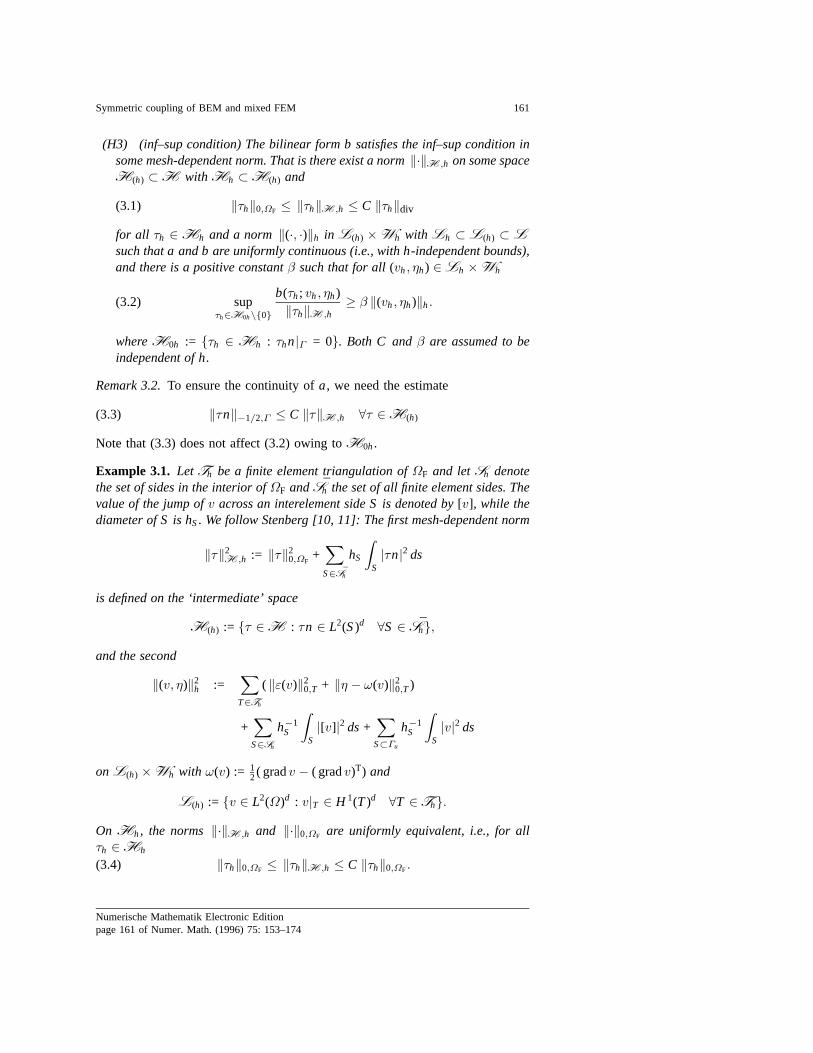
(H3) (inf–sup condition) The bilinear form b satisfies the inf–sup condition insome mesh-dependent norm. That is there exist a norm‖·‖H ,h on some spaceH(h) ⊂ H with Hh ⊂ H(h) and

‖τh‖0,ΩF ≤ ‖τh‖H ,h ≤ C ‖τh‖div(3.1)

for all τh ∈ Hh and a norm‖(·, ·)‖h in L(h) × Wh with Lh ⊂ L(h) ⊂ Lsuch that a and b are uniformly continuous (i.e., with h-independent bounds),and there is a positive constantβ such that for all(vh, ηh) ∈ Lh ×Wh

supτh∈H0h\0

b(τh; vh, ηh)‖τh‖H ,h

≥ β ‖(vh, ηh)‖h.(3.2)

whereH0h := τh ∈ Hh : τhn|Γ = 0. Both C andβ are assumed to beindependent of h.

Remark 3.2.To ensure the continuity ofa, we need the estimate

‖τn‖−1/2,Γ ≤ C ‖τ‖H ,h ∀τ ∈ H(h)(3.3)

Note that (3.3) does not affect (3.2) owing toH0h.

Example 3.1. Let Th be a finite element triangulation ofΩF and letSh denotethe set of sides in the interior ofΩF and ¯Sh the set of all finite element sides. Thevalue of the jump ofv across an interelement side S is denoted by[v], while thediameter of S is hS. We follow Stenberg [10, 11]: The first mesh-dependent norm

‖τ‖2H ,h := ‖τ‖2

0,ΩF+∑

S∈ ¯Sh

hS

∫S|τn|2 ds

is defined on the ‘intermediate’ space

H(h) := τ ∈ H : τn ∈ L2(S)d ∀S ∈ ¯Sh,

and the second

‖(v, η)‖2h :=

∑T∈Th

( ‖ε(v)‖20,T + ‖η − ω(v)‖2

0,T )

+∑

S∈Sh

h−1S

∫S|[v]|2 ds +

∑S⊂Γu

h−1S

∫S|v|2 ds

on L(h) ×Wh with ω(v) := 12( gradv − ( gradv)T) and

L(h) := v ∈ L2(Ω)d : v|T ∈ H 1(T)d ∀T ∈ Th.

On Hh, the norms‖·‖H ,h and ‖·‖0,ΩF are uniformly equivalent, i.e., for allτh ∈ Hh

‖τh‖0,ΩF ≤ ‖τh‖H ,h ≤ C ‖τh‖0,ΩF.(3.4)


162 U. Brink et al.

In these norms, the bilinear forms a and b are continuous, i.e., there exists C> 0such that for all(σ, ϕ), (τ, ψ) ∈ H(h) × H 1/2

a(σ, ϕ; τ, ψ) ≤ C( ‖σ‖H ,h + ‖ϕ‖1/2,Γ )( ‖τ‖H ,h + ‖ψ‖1/2,Γ )(3.5)

and for all (τ, v, η) ∈ H(h) ×L(h) ×W

b(τ ; v, η) ≤ C ‖τ‖H ,h ‖(v, η)‖h.(3.6)

To show continuity of a, it remains to verify(3.3). Recall

‖τn‖−1/2,Γ = supv∈H 1/2(Γ )d

〈τn , v〉‖v‖1/2,Γ

.

Eachv ∈ H 1/2(Γ )d can be extended tov ∈ H 1(ΩF)d with v|Γu = 0 and ‖v‖1,ΩF ≤C ‖v‖1/2,Γ . Integration by parts yields

〈τn , v〉 =∫ΩF

τ : gradv dΩ + b(τ ; v, 0).

Further, ‖(v, 0)‖h ≤ ‖v‖1,ΩF since the jumps[v] on the interelement sides vanish.Thus, using the continuity of b in the mesh-dependent norms, we obtain

〈τn , v〉 ≤ C ‖τ‖H ,h ‖v‖1,ΩF.

This proves(3.3).

Remark 3.3.We assume throughout this paper that the solution to (2.5) satisfiesσ ∈ H(h) and u ∈ L(h) for all f ∈ L2(ΩF)d, which is a regularity condition.In the situation of Example 3.1, the conditionu ∈ H s(ΩF)d with s > 3/2 issufficient.

The discretized saddle point problemconsists in finding (σh, ϕh, uh, γh) ∈Hh× H 1/2

h ×Lh×Wh such that for all (τh, ψh, vh, ηh) ∈ Hh×H 1/2h ×Lh×Wh

a(σh, ϕh; τh, ψh) + b(τh; uh, γh) = 0b(σh; vh, ηh) = − ∫

ΩFf · vh dΩ

(3.7)

Theorem 3.1. Assuming (H1)–(H3), the discrete problem(3.7) has exactly onesolution. There exists some h-independent constant C> 0 such that

‖σ − σh‖H ,h + ‖ϕ− ϕh‖1/2,Γ

≤ C(

infτh∈Hh

‖σ − τh‖H ,h + infψh∈H 1/2

h

‖ϕ− ψh‖1/2,Γ + infηh∈Wh

‖γ − ηh‖0,ΩF

).

To deriveL2-estimates for the displacements, we need a regularity–approxi-mation estimate and a mappingPh : L → Lh ×Wh.



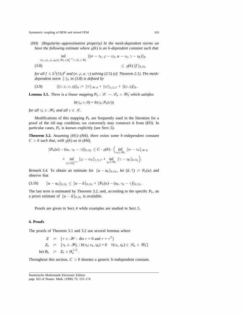
(H4) (Regularity–approximation property) In the mesh-dependent norms wehave the following estimate where%(h) is an h-dependent constant such that

inf(τh,ψh,vh,ηh)∈Hh×H 1/2

h ×Lh×Wh

‖(σ − τh, ϕ− ψh, u − vh, γ − ηh)‖h

≤ %(h) ‖f ‖0,ΩF(3.8)

for all f ∈ L2(ΩF)d and(σ, ϕ, u, γ) solving(2.5) (cf. Theorem 2.1). The mesh-dependent norm‖·‖h in (3.8) is defined by

‖(τ, ψ, v, η)‖h := ‖τ‖H ,h + ‖ψ‖1/2,Γ + ‖(v, η)‖h.(3.9)

Lemma 3.1. There is a linear mapping Ph : L → Lh ×Wh which satisfies

b(τh; v, 0) = b(τh; Ph(v))

for all τh ∈ Hh and all v ∈ L .

Modifications of this mappingPh are frequently used in the literature for aproof of the inf–sup condition; we conversely may construct it from (H3). Inparticular cases,Ph is known explicitly (see Sect. 5).

Theorem 3.2. Assuming (H1)–(H4), there exists some h-independent constantC > 0 such that, with%(h) as in (H4),

‖Ph(u)− (uh, γh − γ)‖0,ΩF ≤ C · %(h) ·(

infτh∈Hh

‖σ − τh‖H ,h

+ infψh∈H 1/2

h



).

Remark 3.4.To obtain an estimate for‖u − uh‖0,ΩF, let (u, γ) := Ph(u) andobserve that

‖u − uh‖0,ΩF ≤ ‖u − u‖0,ΩF + ‖Ph(u)− (uh, γh − γ)‖0,ΩF.(3.10)

The last term is estimated by Theorem 3.2, and, according to the specificPh, ana priori estimate of‖u − u‖0,ΩF is available.

Proofs are given in Sect. 4 while examples are studied in Sect. 5.

4. Proofs

The proofs of Theorem 3.1 and 3.2 use several lemmas where

Z := τ ∈ H : div τ = 0 andτ = τTZh := τh ∈ Hh : b(τh; vh, ηh) = 0 ∀(vh, ηh) ∈ Lh ×Wh

kerBh := Zh × H 1/2h .

Throughout this section,C > 0 denotes a generich-independent constant.


164 U. Brink et al.

Lemma 4.1. [11] For all τh ∈ Zh∫ΩF

τh : C−1τh dΩ ≥ C ‖τh‖20,ΩF

.

Lemma 4.2. For all σ ∈ Z there existsσh ∈ Zh satisfying

‖σ − σh‖div ≤ C infτh∈Hh

‖σ − τh‖0,ΩF.

Proof. The result follows as in [11]; for related results we refer to [3, PropositionII.2.5] and [2, Remark III.4.6]. We give a proof for completeness and to stressthat (H1)–(H3) are sufficient (even for different situations on the boundary). Letσ be the best approximant to ¯σ ∈ Z in Hh with respect to theL2(ΩF)-norm. ByLemma 4.1 and (H3), the mixed finite element problem∫

ΩF

σh : C−1τh dΩ + b(τh; uh, γh) = L1(τh)

b(σh; vh, ηh) = L2(vh, ηh)

(with linear formsL1, L2) satisfies ellipticity and inf–sup conditions in mesh-dependent norms so that we have a unique solution ( ¯σh, uh, γh) ∈ Hh×Lh×Wh

satisfying ∫ΩF

(σh − σ) : C−1τh dΩ + b(τh; uh, γh) = 0(4.1)

b(σh − σ; vh, ηh) = 0(4.2)

for all (τh, vh, ηh) ∈ Hh ×Lh ×Wh. Note that ¯σh − σ ∈ Zh according to (4.2).Hence, Lemma 4.1 yields

C ‖σh − σ‖20,ΩF

≤∫ΩF

(σh − σ) : C−1(σh − σ) dΩ

=∫ΩF

(σ − σ) : C−1(σh − σ) dΩ

owing to (4.1). Thus, by Cauchy’s inequality,

‖σh − σ‖0,ΩF ≤ C ‖σ − σ‖0,ΩF.

Then, the triangle inequality and (H2) finish the proof of the lemma.utLemma 4.3. There is a constantα > 0 such that

inf(σh,ϕh)

sup(τh,ψh)

a(σh, ϕh; τh, ψh)( ‖σh‖H ,h + ‖ϕh‖1/2,Γ )( ‖τh‖H ,h + ‖ψh‖1/2,Γ )

≥ α(4.3)

where the nonzero arguments ininf(σh,ϕh) and sup(τh,ψh) belong tokerBh.



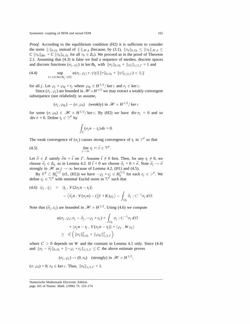
Proof. According to the equilibrium condition (H2) it is sufficient to considerthe norm ‖·‖0,ΩF instead of‖·‖H ,h (because, by (3.1),‖τh‖0,ΩF ≤ ‖τh‖H ,h ≤C ‖τh‖div = C ‖τh‖0,ΩF for all τh ∈ Zh). We proceed as in the proof of Theorem2.1. Assuming that (4.3) is false we find a sequence of meshes, discrete spacesand discrete functions (σj , ϕj ) in kerBhj with ‖σj ‖0,ΩF + ‖ϕj ‖1/2,Γ = 1 and

sup(τ,ψ)∈kerBhj \0

a(σj , ϕj ; τ, ψ)/( ‖τ‖0,ΩF + ‖ψ‖1/2,Γ ) < 1/j(4.4)

for all j . Let ϕj = ϕ0j + rj whereϕ0j ∈ H 1/2/ kerε and rj ∈ kerε.Since (σj , ϕj ) are bounded inH×H 1/2 we may extract a weakly convergent

subsequence (not relabeled); so assume,

(σj , ϕ0j ) (σ, ϕ0) (weakly) in H × H 1/2/ kerε

for some (σ, ϕ0) ∈ H × H 1/2/ kerε. By (H2) we have divσj = 0 and sodivσ = 0. Definetj ∈ Rd by ∫

Γ

(σj n − tj ) ds = 0.

The weak convergence of (σj ) causes strong convergence oftj in Rd so that

limj→∞

tj =: t ∈ Rd.(4.5)

Let σ ∈ Z satisfy σn = t on Γ . Assumet /= 0 first. Then, for anytj /= 0, wechoose ¯σj ∈ Zhj as in Lemma 4.2. Ift = 0 we choose ¯σj = 0 = σ. Note σj → σstrongly inH as j →∞ because of Lemma 4.2, (H1) and (4.5).

By Rd ⊂ H 1/2h (cf., (H1)) we have−ϕj + cj ∈ H 1/2

h for eachcj ∈ Rd. Wedefinecj ∈ Rd with minimal Euclid norm inRd such that

〈cj , tj 〉 = 〈tj , V (2σj n − tj )〉(4.6)

− ⟨σj n , V (σj n)− ( 12I + K )ϕj

⟩− ∫ΩF

σj : C−1σj dΩ.

Note that (σj , cj ) are bounded inH × H 1/2. Using (4.6) we compute

a(σj , ϕj ;σj − σj ,−ϕj + cj ) =∫ΩF

σj : C−1σj dΩ

+ 〈σj n − tj , V (σj n − tj )〉 + 〈ϕj , Wϕj 〉≥ C

(‖σj ‖2

0,ΩF+ ‖ϕ0j ‖2

1/2,Γ

)whereC > 0 depends onW and the constant in Lemma 4.1 only. Since (4.4)and ‖σj − σj ‖0,ΩF + ‖−ϕj + cj ‖1/2,Γ ≤ C the above estimate proves

(σj , ϕj ) → (0, r0) (strongly) inH × H 1/2,

(σ, ϕ0) = 0; r0 ∈ kerε. Thus, ‖r0‖1/2,Γ = 1.


166 U. Brink et al.

Let σ ∈ Z satisfy σn = −r0 on Γ . By Lemma 4.2 we find a discrete stressfield σj ∈ Zhj which, by (H1), converges towards ˆσ in (H , ‖·‖div ). Letting(τ, ψ) := (σj , 0) ∈ kerBhj \ 0 in (4.4),

a(σj , ϕj ; σj , 0)<1j‖σj ‖0,ΩF.

By strong convergence, forj → ∞, a(0, r0; σ, 0) ≤ 0. But, by construction ofσ and because‖r0‖1/2,Γ = 1, a(0, r0; σ, 0) = 〈r0 , r0〉 > 0. This contradictionproves the lemma. utProof of Lemma 3.1.Let Z0

h denote the set of functionalsΦ onHh with Φ(τh) = 0for all τh ∈ Zh. By (H3), the mapping

Lh ×Wh → Z0h

(vh, ηh) 7→ b(·; vh, ηh)

is an isomorphism [2, 3] (assumingLh × Wh be endowed with the mesh-dependent norm). For allv ∈ L , (H2) implies b(·; v, 0)|Hh ∈ Z0

h . Hence, foreachv ∈ L , there existsPh(v) := (vh, ηh) ∈ Lh ×Wh satisfying

b(·; vh, ηh)|Hh = b(·; v, 0)|Hh . ut

Proof of Theorem 3.1.We follow [11, Proof of Theorem 3.1] and let ( ˜σ, ϕ, γ) bethe best approximant to (σ, ϕ, γ) in Hh×H 1/2

h ×Wh. Let Hh×H 1/2h ×Lh×Wh

be endowed with the norm (3.9). Because of (H3) and Lemma 4.3 we get the inf–sup condition for the discrete spaces. With the theory of saddle point problemsthere exists (τh, ψh, vh, ηh) in Hh × H 1/2

h ×Lh ×Wh with

‖(τh, ψh, vh, ηh)‖h ≤ C and

‖σ − σh‖H ,h + ‖ϕ− ϕh‖1/2,Γ + ‖Ph(u)− (uh, γh − γ)‖h

≤ a(σ − σh, ϕ− ϕh; τh, ψh)

+ b(τh; Ph(u)− (uh, γh − γ)) + b(σ − σh; vh, ηh)

= a(σ − σ, ϕ− ϕ; τh, ψh)

+ b(σ − σ; vh, ηh)− b(τh; 0, γ − γ)

where we used the discrete equations andb(τh; Ph(u) − (u, 0)) = 0 according toLemma 3.1. Sincea andb are bounded (in the discrete norms)

‖σ − σh‖H ,h + ‖ϕ− ϕh‖1/2,Γ + ‖Ph(u)− (uh, γh − γ)‖h

≤ C(‖σ − σ‖H ,h + ‖ϕ− ϕ‖1/2,Γ + ‖γ − γ‖0,ΩF

).

This and the triangle inequality prove

‖σ − σh‖H ,h + ‖ϕ− ϕh‖1/2,Γ + ‖Ph(u)− (uh, γh − γ)‖h(4.7)

≤ C(

infτh∈Hh

‖σ − τh‖H ,h + infψh∈H 1/2

h



).



The proof of Theorem 3.1 is finished.ut

Proof of Theorem 3.2.We follow [11], assume (H4) and continue in the notationsof the proof of Theorem 3.1. With Theorem 2.1 we find (Π,Ψ, z, µ) in H ×H 1/2 ×L ×W satisfying, for all (τ, ψ, v, η) in H × H 1/2 ×L ×W ,

a(Π,Ψ ; τ, ψ) + b(τ ; z, µ) = 0

b(Π; v, η) =∫ΩF

(Ph(u)− (uh, γh − γ)

)· (v, η) dΩ.

Taking (τ, ψ, v, η) = (σ − σh, ϕ− ϕh,Ph(u)− (uh, γh − γ)) we obtain

‖Ph(u)− (uh, γh − γ)‖20,ΩF

= b(Π; Ph(u)− (uh, γh − γ))

= a(Π,Ψ ;σ − σh, ϕ− ϕh)

+ b(σ − σh; z, µ) + b(Π; Ph(u)− (uh, γh − γ))

= a(σ − σh, ϕ− ϕh;Π − Π, Ψ − Ψ )

+ b(σ − σh; z − z, µ− µ) + b(Π − Π; Ph(u)− (uh, γh − γ))

using Galerkin equations and the definition ofPh in Lemma 3.1 for the bestapproximants (Π, Ψ , z, µ) in Hh×H 1/2

h ×Lh×Wh to (Π,Ψ, z, µ). Consideringnorms and using (4.7) forσ − σh, ϕ− ϕh andPh(u)− (uh, γh − γ) we gain

‖Ph(u)− (uh, γh − γ)‖20,ΩF

≤ C · ‖(Π − Π, Ψ − Ψ , z − z, µ− µ)‖h

· ( ‖σ − σ‖H ,h + ‖ϕ− ϕ‖1/2,Γ + ‖γ − γ‖0,ΩF).

By (H4), we have an a priori estimate of the form

‖(Π − Π, Ψ − Ψ , z − z, µ− µ)‖h ≤ %(h) ‖Ph(u)− (uh, γh − γ)‖0,ΩF.

Using this in the former estimate and dividing by‖Ph(u)− (uh, γh − γ)‖0,ΩF weconclude the claimed estimate.ut

5. A family of elements

In the sequel we describe a family of finite element spaces due to Stenberg [11].For each tetrahedron (resp. triangle)T ∈ Th we define a bubble functionbT by

bT (x) =d∏

i =0

λi (x) ,

whereλ0, . . . , λd are the barycentric coordinates inT. By Pk(T) we denote thespace of polynomials of degree≤ k on T. For d = 3 we define

Bl (T) := (τij ) : (τi 1, . . . , τi 3) = curl (bTwi 1, . . . , bTwi 3),

wij ∈ Pl (T), i , j = 1, 2, 3


168 U. Brink et al.

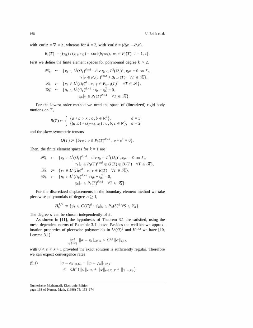
with curlz = ∇× z, whereas ford = 2, with curlz = (∂2z,−∂1z),

Bl (T) := (τij ) : (τi 1, τi 2) = curl (bTwi ), wi ∈ Pl (T), i = 1, 2.First we define the finite element spaces for polynomial degreek ≥ 2,

Hh := τh ∈ L2(ΩF)d×d : div τh ∈ L2(ΩF)d, τhn = 0 onΓt ,

τh|T ∈ Pk(T)d×d + Bk−1(T) ∀T ∈ Th,Lh := vh ∈ L2(ΩF)d : vh|T ∈ Pk−1(T)d ∀T ∈ Th,Wh := ηh ∈ L2(ΩF)d×d : ηh + ηT

h = 0,

ηh|T ∈ Pk(T)d×d ∀T ∈ Th.For the lowest order method we need the space of (linearized) rigid body

motions onT,

R(T) :=

a + b × x : a, b ∈ R3, d = 3,(a, b) + c(−x2, x1) : a, b, c ∈ R, d = 2,

and the skew-symmetric tensors

Q(T) := bT% : % ∈ P0(T)d×d , % + %T = 0.Then, the finite element spaces fork = 1 are

Hh := τh ∈ L2(ΩF)d×d : div τh ∈ L2(ΩF)d, τhn = 0 onΓt ,

τh|T ∈ P1(T)d×d ⊕Q(T)⊕ B0(T) ∀T ∈ Th,Lh := vh ∈ L2(ΩF)d : vh|T ∈ R(T) ∀T ∈ Th,Wh := ηh ∈ L2(ΩF)d×d : ηh + ηT

h = 0,

ηh|T ∈ P1(T)d×d ∀T ∈ Th.For the discretized displacements in the boundary element method we take

piecewise polynomials of degreeκ ≥ 1,

H 1/2h := ψh ∈ C(Γ )d : ψh|S ∈ Pκ(S)d ∀S ∈ Eh.

The degreeκ can be chosen independently ofk.As shown in [11], the hypotheses of Theorem 3.1 are satisfied, using the

mesh-dependent norms of Example 3.1 above. Besides the well-known approx-imation properties of piecewise polynomials inL2(Ω)d and H 1/2 we have [10,Lemma 3.1]

infτh∈Hh

‖σ − τh‖H ,h ≤ Chs ‖σ‖s,ΩF

with 0≤ s ≤ k + 1 provided the exact solution is sufficiently regular. Thereforewe can expect convergence rates

‖σ − σh‖0,ΩF + ‖ϕ− ϕh‖1/2,Γ(5.1)

≤ Chs( ‖σ‖s,ΩF + ‖ϕ‖s+1/2,Γ + ‖γ‖s,ΩF

)



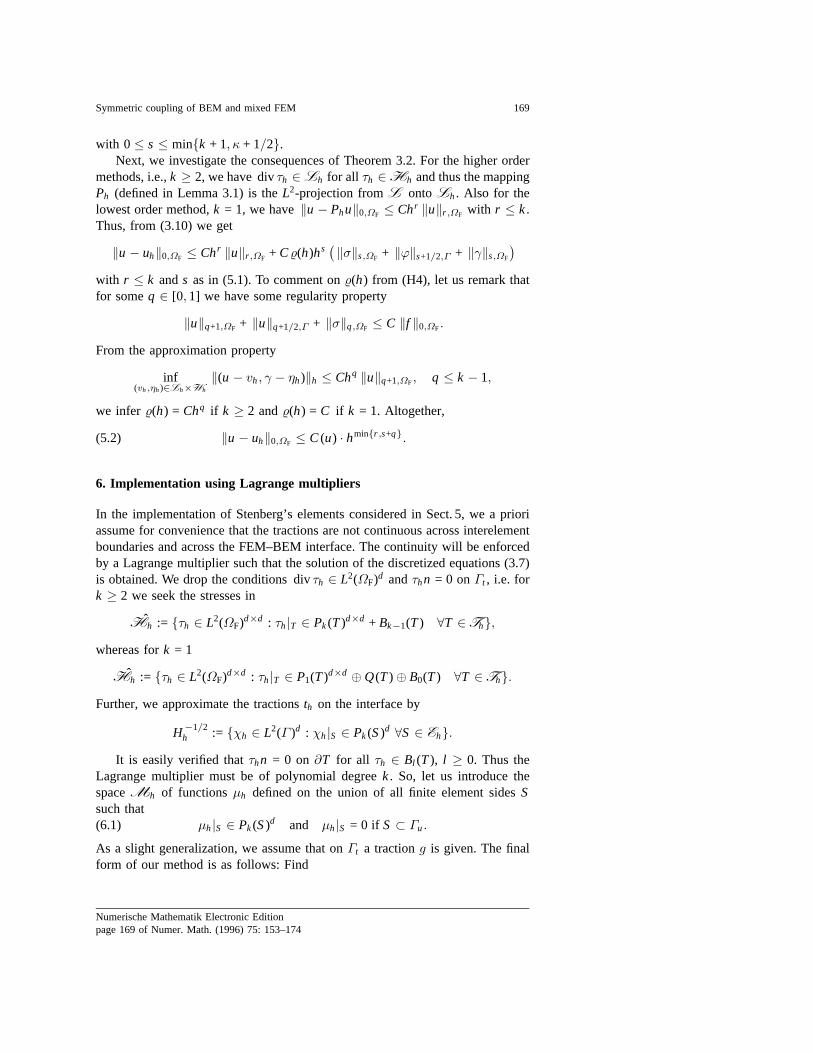
with 0≤ s ≤ mink + 1, κ + 1/2.Next, we investigate the consequences of Theorem 3.2. For the higher order

methods, i.e.,k ≥ 2, we have divτh ∈ Lh for all τh ∈ Hh and thus the mappingPh (defined in Lemma 3.1) is theL2-projection fromL onto Lh. Also for thelowest order method,k = 1, we have‖u − Phu‖0,ΩF ≤ Chr ‖u‖r ,ΩF with r ≤ k.Thus, from (3.10) we get

‖u − uh‖0,ΩF ≤ Chr ‖u‖r ,ΩF + C%(h)hs( ‖σ‖s,ΩF + ‖ϕ‖s+1/2,Γ + ‖γ‖s,ΩF

)with r ≤ k ands as in (5.1). To comment on%(h) from (H4), let us remark thatfor someq ∈ [0, 1] we have some regularity property

‖u‖q+1,ΩF + ‖u‖q+1/2,Γ + ‖σ‖q,ΩF ≤ C ‖f ‖0,ΩF.

From the approximation property

inf(vh,ηh)∈Lh×Wh

‖(u − vh, γ − ηh)‖h ≤ Chq ‖u‖q+1,ΩF, q ≤ k − 1,

we infer %(h) = Chq if k ≥ 2 and%(h) = C if k = 1. Altogether,

‖u − uh‖0,ΩF ≤ C(u) · hminr ,s+q.(5.2)

6. Implementation using Lagrange multipliers

In the implementation of Stenberg’s elements considered in Sect. 5, we a prioriassume for convenience that the tractions are not continuous across interelementboundaries and across the FEM–BEM interface. The continuity will be enforcedby a Lagrange multiplier such that the solution of the discretized equations (3.7)is obtained. We drop the conditions divτh ∈ L2(ΩF)d andτhn = 0 onΓt , i.e. fork ≥ 2 we seek the stresses in

Hh := τh ∈ L2(ΩF)d×d : τh|T ∈ Pk(T)d×d + Bk−1(T) ∀T ∈ Th,whereas fork = 1

Hh := τh ∈ L2(ΩF)d×d : τh|T ∈ P1(T)d×d ⊕Q(T)⊕ B0(T) ∀T ∈ Th.Further, we approximate the tractionsth on the interface by

H−1/2h := χh ∈ L2(Γ )d : χh|S ∈ Pk(S)d ∀S ∈ Eh.

It is easily verified thatτhn = 0 on ∂T for all τh ∈ Bl (T), l ≥ 0. Thus theLagrange multiplier must be of polynomial degreek. So, let us introduce thespaceMh of functionsµh defined on the union of all finite element sidesSsuch that

µh|S ∈ Pk(S)d and µh|S = 0 if S ⊂ Γu.(6.1)

As a slight generalization, we assume that onΓt a tractiong is given. The finalform of our method is as follows: Find


170 U. Brink et al.

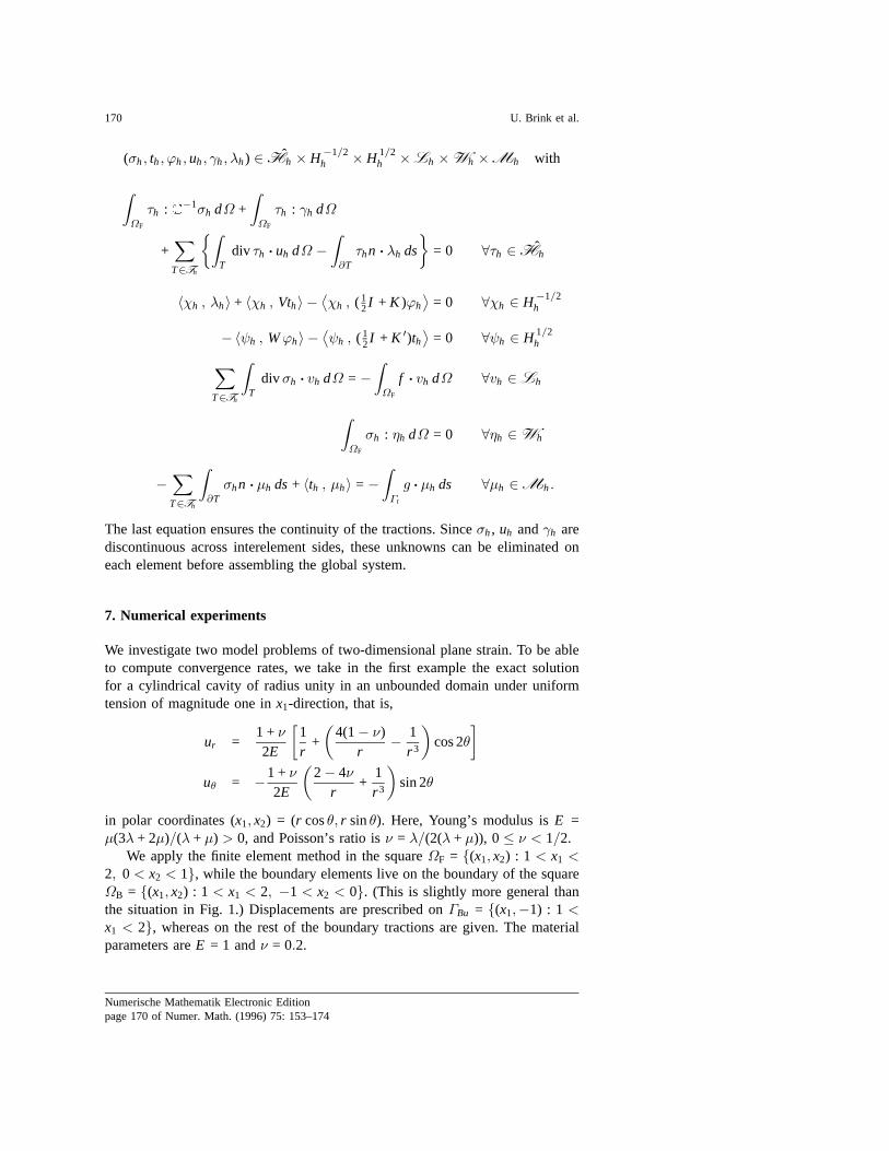
(σh, th, ϕh, uh, γh, λh) ∈ Hh × H−1/2h × H 1/2

h ×Lh ×Wh ×Mh with

∫ΩF

τh : C−1σh dΩ +∫ΩF

τh : γh dΩ

+∑

T∈Th

∫T

div τh · uh dΩ −∫∂Tτhn · λh ds

= 0 ∀τh ∈ Hh

〈χh , λh〉 + 〈χh , Vth〉 −⟨χh , ( 1

2I + K )ϕh⟩

= 0 ∀χh ∈ H−1/2h

−〈ψh , Wϕh〉 −⟨ψh , ( 1

2I + K ′)th⟩

= 0 ∀ψh ∈ H 1/2h∑

T∈Th

∫T

divσh · vh dΩ = −∫ΩF

f · vh dΩ ∀vh ∈ Lh

∫ΩF

σh : ηh dΩ = 0 ∀ηh ∈ Wh

−∑

T∈Th

∫∂Tσhn · µh ds + 〈th , µh〉 = −

∫Γt

g · µh ds ∀µh ∈ Mh.

The last equation ensures the continuity of the tractions. Sinceσh, uh andγh arediscontinuous across interelement sides, these unknowns can be eliminated oneach element before assembling the global system.

7. Numerical experiments

We investigate two model problems of two-dimensional plane strain. To be ableto compute convergence rates, we take in the first example the exact solutionfor a cylindrical cavity of radius unity in an unbounded domain under uniformtension of magnitude one inx1-direction, that is,

ur =1 +ν2E

[1r

+

(4(1− ν)

r− 1

r 3

)cos 2θ

]uθ = −1 +ν

2E

(2− 4ν

r+

1r 3

)sin 2θ

in polar coordinates (x1, x2) = (r cosθ, r sinθ). Here, Young’s modulus isE =µ(3λ + 2µ)/(λ + µ) > 0, and Poisson’s ratio isν = λ/(2(λ + µ)), 0≤ ν < 1/2.

We apply the finite element method in the squareΩF = (x1, x2) : 1 < x1 <2, 0< x2 < 1, while the boundary elements live on the boundary of the squareΩB = (x1, x2) : 1 < x1 < 2, −1 < x2 < 0. (This is slightly more general thanthe situation in Fig. 1.) Displacements are prescribed onΓBu = (x1,−1) : 1 <x1 < 2, whereas on the rest of the boundary tractions are given. The materialparameters areE = 1 andν = 0.2.



We use the lowest order method of Sect. 5 with polynomial degreesk = 1andκ = 1. The meshes are uniform (as in Example 2, Fig. 3). Each refinementstep is performed by halving all sides and all boundary elements. In Table 1,Ndenotes the number of finite elements inΩF, CR is the convergence rate andREis the relative error in theL2-norm, i.e.,

‖σ − σh‖0,ΩF

‖σ‖0,ΩF

for σh,‖u − uh‖0,ΩF

‖u‖0,ΩF

for uh,‖ϕ− ϕh‖0,Γ

‖ϕ‖0,Γfor ϕh,

respectively, whereΓ := ∂ΩB \ ΓBu.

Table 1. Example 1, errors forν = 0.2

σh uh ϕh

N RE CR RE CR RE CR

8 .1184 .07130 .0204332 .03951 1.58 .03333 1.10 .004352 2.23128 .01153 1.78 .01651 1.01 .001049 2.05512 .003135 1.88 .008228 1.01 .0002587 2.022048 .0008170 1.94 .004110 1.00 .00006447 2.00

Table 2. Example 1, errors forν = 0.4998

σh uh ϕh

N RE CR RE CR RE CR

8 .1190 .07480 .0220532 .03969 1.58 .03714 1.01 .005533 1.99128 .01159 1.78 .01832 1.02 .001294 2.10512 .003144 1.88 .009122 1.01 .0003087 2.072048 .0008188 1.94 .004556 1.00 .00007019 2.14

Since the solution is smooth, the convergence rates depend onk andκ only.The computed convergence rates tend to the optimal values that can be expectedfrom the approximation properties. Forσh andϕh the results are better than thevalue 3/2 predicted by (5.1). The convergence rates foruh agree with (5.2). Onless uniform meshes, the results are similar.

Forν = 0.4998, i.e. almost incompressible material, the relative error is nearlyunchanged as seen in Table 2. This is in contrast to the poor behavior of standard(displacement) finite element methods as confirmed by numerical experiments in[8] where the above lowest order finite element method is compared with otherstandard and mixed approaches.

Inside the BEM domain, the stresses converge with higher order as Table 3shows for the sampling pointsP1 = (0.3,−0.2) andP2 = (0.3,−0.7). This is acharacteristic feature of boundary element methods.

In the second example, we take a solution with a singularity typically arisingat a re-entrant corner. Using again polar coordinates (r , θ), −π < θ ≤ π, we


172 U. Brink et al.

6

-

@@@@

@@@@@@@@@@@@

2

1

0

−1

−2

−1 0 1 2x1

x2

ΩF

FEM

ΩB

BEM

Γ

A

B

C

D

Singularity at (0, 0);displacements prescribed on side AB,elsewhere tractions given.

Fig. 2. Example 2

Fig. 3. Mesh and deformations for Example 2 (128 finite elements, 48 boundary elements)

impose the boundary conditionsσn = 0 for θ = ±ω whereω is half of theinterior angle at the corner. According to [12], for plane strain,

ur =1

2µrα −(α + 1)C1 cos((α + 1)θ) + (C3 − (α + 1))C2 cos((α− 1)θ)

uθ =1

2µrα (α + 1)C1 sin((α + 1)θ) + (C3 + α− 1)C2 sin((α− 1)θ)

σr = rα−1−α(α + 1)C1 cos((α + 1)θ) + α(3− α)C2 cos((α− 1)θ)σθ = rα−1α(α + 1)C1 cos((α + 1)θ) + C2 cos((α− 1)θ)σrθ = rα−1α(α + 1)C1 sin((α + 1)θ) + (α− 1))C2 sin((α− 1)θ)

whereα solvesα sin 2ω + sin(2ωα) = 0.(7.1)

The constantC1 is arbitrary,C2 = −C1 cos((α + 1)ω)/ cos((α − 1)ω) and C3 =2(λ + 2µ)/(λ + µ), λ andµ denoting the Lame coefficients. In our example (see



0

2

4

6

8

10

-1 -0.8 -0.6 -0.4 -0.2 0

Firs

t prin

cipa

l str

ess

x1-coordinate

2 edges on CD4 edges on CD8 edges on CD

16 edges on CDexact

Fig. 4. Example 2, first principal stress on the side CD

Table 3. Example 1, stresses inside the BEM domain forν = 0.2

σh(P1) σh(P2)

N RE CR RE CR

8 .6069E–1 .4031E–132 .7739E–3 6.29 .3168E–2 3.67128 .3444E–3 1.17 .1984E–3 4.00512 .3856E–4 3.16 .4027E–4 2.302048 .4301E–5 3.16 .1104E–4 1.87

Fig. 2) we haveω = 3π/4. Since we are interested in the most singular part ofu,we take the smallest positive solution of (7.1), i.e.α = 0.544483736782463929....

In the computations we chooseC1 = 1 andλ andµ corresponding toE = 100,ν = 0.3. Further, we add a rigid body movement inx1-direction such thatu = 0at the point (2, 0). Again we employ the lowest order method (k = 1, κ = 1) onuniform meshes.

Since nowu ∈ H 1+α−ε(Ω) for all ε > 0, the estimates (5.1) and (5.2) predictthe convergence rateα. The numerical results forσh are in good agreement withthis value (see Table 4).

In general, if a singularity is present, the convergence rates foruh andϕh

cannot be expected to tend to a higher value than forσh. This is confirmed bynumerical experiments withC2 different from the above value; then, however,‘artificial’ boundary conditions forσn on the wedgeθ = ±ω are applied.

Computed deformations are shown in Fig. 3. In the FEM domain, as anapproximation tou the Lagrange multipliersλh of Sect. 6 are used, with averaged


174 U. Brink et al.

Table 4. Errors for Example 2

σh uh ϕh

N RE CR RE CR RE CR

8 .2090 .1084 .0576332 .1413 0.5658 .04848 1.16 .02771 1.06128 .09684 0.5456 .02344 1.05 .01341 1.05512 .06640 0.5449 .01155 1.02 .006496 1.052048 .04552 0.5447 .005725 1.01 .003149 1.048192 .03121 0.5446 .002845 1.01 .001527 1.04

values at the vertices of the triangles. Figure 4 shows the first principal stressalong the side CD (indicated in Fig. 2). The values clearly tend towards the exactsolution when the mesh is refined.

Acknowledgement.We are indebted to M. Maischak (Institut fur Angewandte Mathematik, Uni-versitat Hannover) for lending BEM-integration routines. The research of the first and third authorwas supported by the German Research Foundation (DFG) within the Priority Research Program‘Boundary Element Methods’ under Grant No. Ste 238/19-3.

References

1. Arnold, D. N., Brezzi, F., Douglas, J. (1984): PEERS : A new mixed finite element for planeelasticity. Japan J. Appl. Math.1, 347–367

2. Braess, D. (1992): Finite Elemente – Theorie, schnelle Loser und Anwendungen in der Elas-tiztitatstheorie. Springer, Berlin

3. Brezzi, F., Fortin, M. (1991): Mixed and Hybrid Finite Element Methods. Springer, New York4. Carstensen, C. (1993): Interface problem in holonomic elastoplasticity. Math. Meth. Appl. Sci.

16, 819–8355. Costabel, M. (1988): Boundary integral operators on Lipschitz domains: Elementary results.

SIAM J. Math. Anal.19, 613–6266. Costabel, M. (1988): A symmetric method for the coupling of finite elements and boundary

elements. In: J. R. Whiteman, ed., The Mathematics of Finite Elements and Applications IV,MAFELAP 1987, pp. 281–288. Academic, London

7. Costabel, M., Stephan, E. P. (1990): Coupling of finite and boundary element methods for anelastoplastic interface problem. SIAM J. Numer. Anal.27, 1212–1226

8. Klaas, O., Schroder, J., Stein, E., Miehe, C. (1995): A regularized dual mixed element for planeelasticity – Implementation and performance of the BDM-Element. Comput. Methods Appl.Mech. Engrg. 121, 201–209

9. Pitkaranta, J., Stenberg, R. (1983): Analysis of some mixed finite element methods for planeelasticity equations. Math. Comp.41, 399–423

10. Stenberg, R. (1986): On the construction of optimal mixed finite element methods for the linearelasticity problem. Numer. Math.48, 447–462

11. Stenberg, R. (1988): A family of mixed finite elements for the elasticity problem. Numer. Math.53, 513–538

12. Williams, M. L. (1952): Stress singularities resulting from various boundary conditions in angularcorners of plates in extension. J. Appl. Mech.19, 526–528

This article was processed by the author using the LaTEX style file pljour1m from Springer-Verlag.


Documents

Numerische Mathematik - hu-berlin.decc/cc_homepage/download/1996-BU_CC_SE...Numer. Math. (1996) 75: 153–174 Numerische Mathematik c Springer-Verlag 1996 Electronic Edition Symmetric