UNIVERSITI PUTRA MALAYSIA

PADDY FIELD ZONE DELINEATION USING APPARENT ELECTRICAL CONDUCTIVITY AND ITS RELATIONSHIP TO THE

CHEMICAL AND PHYSICAL PROPERTIES OF SOIL

AIMRUN WAYAYOK.

ITMA 2006 6

PADDY FIELD ZONE DELINEATION USING APPARENT ELECTRICAL CONDUCTIVITY AND ITS RELATIONSHIP TO THE CHEMICAL AND

PHYSICAL PROPERTIES OF SOIL

BY

AIMRUN WAYAYOK

Thesis Submitted to the School of Graduate Studies, Universiti Putra Malaysia, in Fulfilment of the Requirement for the Degree of Doctor of Philosophy

March 2006

Dedication

From the depth of my heart, I dedicate this thesis to my beloved father Abdul

Kimlee, mother Sapiyah, sisters Manisa and Warda, and brothers Mustafa, Sulaiman,

Abdul Hadi and Anwar.

Abstract of thesis presented to the Senate of Universiti Putra Malaysia in fulfilment of the requirement for the degree of Doctor of Philosophy

PADDY FIELD ZONE DELINEATION USING APPARENT ELECTRICAL CONDUCTIVITY AND ITS RELATIONSHIP TO THE CHEMICAL AND

PHYSICAL PROPERTIES OF SOIL

AIMRUN WAYAYOK

March 2006

Chairman: Professor Ir. Mohd Amin Mohd Soom, PhD

Institute: Advanced Technology

Spatial variability and temporal variability of soil chemical and physical properties

within a field is unavoidable. Meanwhile, laboratory soil test is usually time

consuming and laborious. To satisfy the concept of precision farming, rapid and

intensive soil sampling is necessary for describing the uncertainty within a field.

Apparent or bulk soil electrical conductivity (EC,) technique for describing soil

spatial variability is widely used. A sensor known as VerisEC can measure the

average EC, of 0-30 cm (shallow EC,) and 0-90 cm (deep EC,) depths and locate its

position by Differential Global Positioning System (DGPS) at every second. EC,

includes soil salinity and soil texture. Soil texture has high correlation with soil

cation exchange capacity (CEC) hence, soil nutrient contents. The main purpose of

this study was to generate variability map of soil EC, within rice cultivation areas

using VerisEC sensor for three seasons. The EC, values were then compared to some

soil chemical and physical properties namely pH, EC, OM, OC, total S, total N,

available P, CEC, Ca, Mg, K, Na, Al, Fe, total cation, BS, ESP, dry bulk density,

moisture content, clay, silt, fine sand, coarse sand and sand, within classes after

delineation. The study site was 145 ha paddy fields at Block C, Sawah Sempadan in

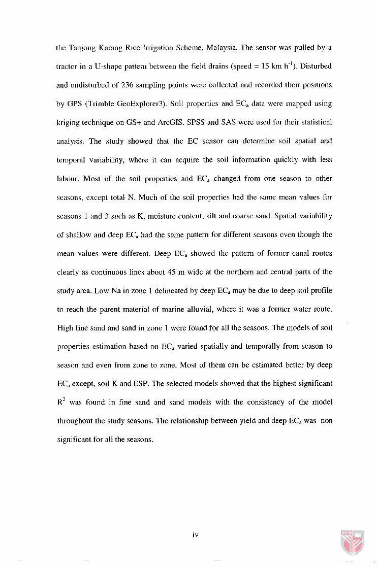
the Tanjong Karang Rice Irrigation Scheme, Malaysia. The sensor was pulled by a

tractor in a U-shape pattern between the field drains (speed = 15 km h-'). Disturbed

and undisturbed of 236 sampling points were collected and recorded their positions

by GPS (Trimble GeoExplorer3). Soil properties and EC, data were mapped using

kriging technique on GS+ and ArcGIS. SPSS and SAS were used for their statistical

analysis. The study showed that the EC sensor can determine soil spatial and

temporal variability, where it can acquire the soil information quickly with less

labour. Most of the soil properties and EC, changed from one season to other

seasons, except total N. Much of the soil properties had the same mean values for

seasons 1 and 3 such as K, moisture content, silt and coarse sand. Spatial variability

of shallow and deep EC, had the same pattern for different seasons even though the

mean values were different. Deep EC, showed the pattern of former canal routes

clearly as continuous lines about 45 m wide at the northern and central parts of the

study area. Low Na in zone 1 delineated by deep EC, may be due to deep soil profile

to reach the parent material of marine alluvial, where it was a former water route.

High fine sand and sand in zone 1 were found for all the seasons. The models of soil

properties estimation based on EC, varied spatially and temporally from season to

season and even from zone to zone. Most of them can be estimated better by deep

EC, except, soil K and ESP. The selected models showed that the highest significant

R* was found in fine sand and sand models with the consistency of the model

throughout the study seasons. The relationship between yield and deep EC, was non

significant for all the seasons.

WUSTAKAAN SULTAN A W L SAM40 UNIVEESITI PUTiiA Fd ' '::!A

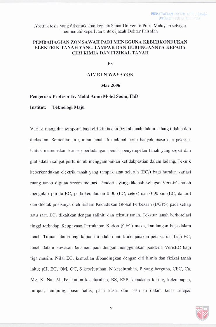
Abstrak tesis yang dikemukakan kepada Senat Universiti Putra Malaysia sebagai memenuhi keperluan untuk ijazah Doktor Falsafah

PEMBAHAGIAN ZON SAWAH PAD1 MENGGUNA KEBERKONDUKAN ELEKTRIK TANAH YANG TAMPAK DAN HUBUNGANNYA KEPADA

CIRI KIMIA DAN FIZIKAL TANAH

AIMRUN WAYAYOK

Mac 2006

Pengerusi: Profesor Ir. Mohd Amin Mohd Soom, PhD

Institut: Teknologi Maju

Variasi ruang dan temporal bagi ciri kimia dan fizikal tanah dalam ladang tidak boleh

dielakkan. Sementara itu, ujian tanah di makmal perlu banyak masa dan pekerja.

Untuk memuaskan konsep perladangan persis, penyempelan tanah yang cepat dan

giat adalah sangat perlu untuk menggambarkan ketidakpastian dalam Iadang. Teknik

keberkondukan elektrik tanah yang tampak atau seluruh (EC,) bagi huraian variasi

ruang tanah diguna secara meluas. Penderia yang dikenali sebagai VerisEC boleh

mengukur purata EC, pada kedalaman 0-30 (EC, cetek) dan 0-90 sm (EC, dalarn)

dan diletak posisinya oleh Sistem Kedudukan Global Perbezaan (DGPS) pada setiap

satu saat. EC, dikaitkan dengan saliniti dan tekstur tanah. Tekstur tanah berkorelasi

tinggi terhadap Keupayaan Pertukaran Kation (CEC) maka, kandungan baja dalarn

tanah. Tujuan utama bagi kajian ini adalah untuk menjanakan peta variasi bagi EC,

tanah dalam kawasan tanaman padi dengan menggunakan penderia VerisEC bagi

tiga musim. Nilai EC, kemudian dibandingkan dengan ciri kimia dan fizikal tanah

iaitu; pH, EC, OM, OC, S keseluruhan, N keseluruhan, P yang berguna, CEC, Ca,

Mg, K, Na, Al, Fe, kation keseluruhan, BS, ESP, kepadatan kering, kelembapan,

lumpur, lempung, pasir halus, pasir kasar dan pasir di dalam kelas selepas

dibahagikan. Kawasan kajian ini adalah di ladang padi seluas 145 ha terletak di Blok

C, Sawah Sempadan dalam Skim Pengairan Padi Tanjong Karang, Malaysia.

Penderia telah ditarik dengan traktor berbentuk U diantara parit tengah (kalajuan =

15 km j-'). Titik sampel yang terganggu dan tidak terganggu bagi 236 sampel telah

dikutip dan dirakamkan lokasinya oleh GPS (Trimble GeoExplorer3). Data ciri tanah

dan EC, telah dijanakan peta menggunakan teknik kriging diatas GS+ dan ArcGIS.

SPSS dan SAS telah diguna untuk analisa statistik. Kajian ini menunjuk bahawa

penderia EC boleh menentukan variasi ruang dan temporal tanah dimana ia boleh

memperoleh maklumat tanah dengan cepat dengan kurang pekerja. Kebanyakan ciri

tanah dan EC, berubah dari satu musim ke satu musim yang lain melainkan, N

keseluruhan. Banyak ciri tanah mengandungi nilai purata yang sama bagi musim 1

dan 3 seperti K, kelembapan, lempung dan pasir kasar. Variasi ruang bagi EC, yang

cetek dan dalam mempunyai bentuk yang sama bagi musim yang berbeza walaupun

nilai puratanya berbeza. EC, dalam menunjuk bentuk laluan sungai lama dengan

jelas seperti garisan sambungan seluas 45 m di sebelah utara dan kawasan tengah

bagi kawasan kajian. Na yang rendah di zon 1 yang dibahagikan oleh EC, dalam

munkin disebabkan oleh profil tanah yang dalam untuk mencapai bahan asas Ianar

laut. Kandungan pasir halus dan pasir yang tinggi dalam zon 1 terdapat pada semua

musim. Model anggaran ciri tanah berasaskan EC, berbeza secara ruang atau

temporal dari satu musim ke satu musim yang lain atau satu zon ke satu zon yang

lain. Banyak ciri tanah baik dianggar oleh EC, dalam malainkan, K dan ESP. Model

yang terpilih menunjukkan bahawa R' yang penting yang paling tinggi adalah

terdapat pada model pasir halus dan pasir dengan model yang konsisten pada semua

musim kajian. Hubungan diantara hasil dan EC, dalam adalah tidak penting bagi

semua musirn.

ACKNOWLEDGEMENTS

First of all, I am thankful to Allah Almighty for making all things possible,

Alhamdulillah.

I would like to express my sincere gratitude to my supervisor, Prof. Ir. Dr. Mohd.

Amin Mohd. Soom, for his untiring guidance, advice, support and encouragement

throughout my study program. I am very grateful to the members of my supervisory

committee, Prof. Ir. Dr. Desa Ahmad and Assoc. Prof. Dr. Mohd. Hanafi Musa, for

their valuable suggestions to complete the study. Special thanks to Dr. S. Osmanu

(Ghana) for his valuable suggestions and reviewing of this manuscript.

I am very grateful to the Malaysian Centre for Remote Sensing (MACRES) for

providing the opportunity to be part of the Precision Farming research group. I am

thankful to Mr. Ezrin Mohd Husin (Science Officer at ITMA) for his assistance, and

also not forgetting all Soil Analysis laboratory staff, the Department of Agriculture

(DOA) for their valuable assistance in analyzing soil properties. Special thanks to

Hjh. Faridah Ahmad for her support and assistance.

I would like to express my special thanks to all of my friends and colleagues: Md

Rowshon Kamal (Bangladesh), Ahmed Ibrahim Khmaj (Libya), Mustafa Yusif

(Sudan), Rusnam Mansur (Indonesia) and Hassan Saad Mohd Hilrni (Sudan),

Abdullah and Yousif (Saudi Arabia) and others who are not mentioned here, for their

moral support during my study.

Lastly, I would like to extend my heartfelt thanks to my parents, brothers and sisters

for their love, understanding and encouragement to complete this study.

vii

I certify that an Examination Committee has met on 27th March 2006 to conduct the final examination of Aimrun Wayayok on his Doctor of Philosophy thesis entitled "Paddy Field Zone Delineation using Apparent Electrical Conductivity and its Relationship to the Chemical and Physical Properties of Soil" in accordance with Universiti Pertanian Malaysia (Higher Degree) Act 1980 and Universiti Pertanian Malaysia (Higher Degree) Regulations 1981. The Committee recommends that the candidate be awarded the relevant degree. Members of the Examination Committee are as follows:

Wan Ishak Wan Ismail, PhD Professor Institute of Advanced Technology Universiti Putra Malaysia (Chairman)

Anuar Abdul Rahim, PhD Associate Professor Faculty of Agriculture Universiti Putra Malaysia (Internal Examiner)

Asep Sapei, PhD Lecturer Faculty of Engineering Universiti Putra Malaysia (Internal Examiner)

Wan Sulaiman Wan Harun, PhD Professor Faculty of Resource Science and Technology Universiti Malaysia Sarawak (External Examiner)

Professor/Deputy ~ e a n School of Graduate Studies Universiti Putra Malaysia

Date : 15 JUN 2006

. . . V l l l

This thesis submitted to the Senate of Universiti Putra Malaysia and has been accepted as fulfilment of the requirement for the degree of Doctor of Philosophy. The members ofthe Supervisory Committee are as follows:

Mohd Amin Mohd Soom, PhD, PEng Professor Faculty of Engineering Universiti Putra Malaysia (Chairman)

Desa Ahmad, PhD, PEng Professor Faculty of Engineering Universiti Putra Malaysia (Member)

Mohd Hanafi Musa, PhD Associate Professor Faculty of Agriculture Universiti Putra Malaysia (Member)

AINI IDEIUS, PhD ProfessorDean School of Graduate Studies Universiti Putra Malaysia

Date: 13 JUL 2006

DECLARATION

I hereby declare that the thesis is based on my original work except for quotations and citations which have been duly acknowledged. I also declare that it has not been previously or currently submitted for any other degree at UPM or other institutions.

AIMRUN WAYAYOK

Date: 1 2 . 0 ~ ~

TABLE OF CONTENTS

DEDICATION ABSTRACT ABSTRAK ACKNOWLEDGEMENTS APPROVAL APPROVAL DECRALATION LIST OF TABLES LIST OF FIGURES LIST OF ABBREVIATIONS

CHAPTER

1 INTRODUCTION 1.1 Introduction 1.2 Statement of the Problems 1.3 Objectives 1.4 Scope of the Study

Page . . 11 ... 111

v vii ...

Vl l l

ix X

xiv XX

xxv

LITERATURE REVIEW 2.1 Introduction 2.2 Basic Knowledge for Electrical Conductivity 2.3 Global Positioning System

2.3.1 GPS System Overview 2.3.2 Basic Idea about GPS

2.4 Geographical Information System and Geospatial Data 2.4.1 The Importance of Geospatial Data 2.4.2 GIs in Agriculture

2.5. Precision Farming 2.5.1 History of Precision Farming 2.5.2 Precision and Accuracy 2.5.3 Spatial Autocorrelation 2.5.4 Management Zone 2.5.5 Zone Delineation 2.5.6 Interpolation Techniques and Variogram

Analysis 2.6 Electrical Conductivity Map and Its Uses 2.7 Relationship between EC and Soil Properties

2.7.1 LabEC

2.7.2 In-Situ or Field EC, 2.8 Variable Rate Technology

2.8.1 Map-based Technologies 2.8.2 Sensor-based Technologies

2.9 Rice Cultivation 2.9.1 Soil and Fertilizer management 2.9.2 Water

2.10 Summary

METHODOLOGY 3.1 Study Area

3.1.1 Location and Topography 3.1.2 Soil Characteristics

3.2 Duration of Field Works 3.3 EC, Data Acquisition and Map Generation 3.4 Soil Sampling, Lab Analysis and Soil Map

Generation 3.4.1 Physical Properties 3.4.2 Chemical Properties

3.5 Yield Data 3.6 Classical Statistical Analysis for EC, and Soil

Data 3.7 Mapping of Soil Properties 3.8 Modeling of Soil Properties

RESULTS AND DISCUSSION 4.1 Introduction 4.2 Statistical Description

4.2.1 Bulk Soil Electrical Conductivity 4.2.2 Chemical Properties 4.2.3 Physical Properties

4.3 Temporal Variability 4.3.1 Bulk Soil Electrical Conductivity 4.3.2 Chemical Properties 4.3.3 Physical Properties

4.4 Geostatistics Description 4.4.1 Bulk Soil Electrical Conductivity 4.4.2 Chemical Properties 4.4.3 Physical Properties

4.5 Spatial Variability 4.5.1 Bulk Soil Electrical Conductivity 4.5.2 Chemicals Properties 4.5 -3 Physicals Properties

4.6 Matrix Correlation of Soil Properties

xii

4.7 EC, Zonal Characteristics 4.7.1 Shallow EC, Zones 4.7.2 Deep EC, Zones

4.8 Model for Soil Property Estimations 4.8.1 For the Entire Study Area 4.8.2 Forthezones

4.9 Soil Properties Affecting EC, 4.9.1 Entire Study Area 4.9.2 For the Zones

4.10 EC, and Yield Characteristics

CONCLUSIONS

REFERENCES APPENDICES BIODATA OF THE AUTHOR

... X l l l

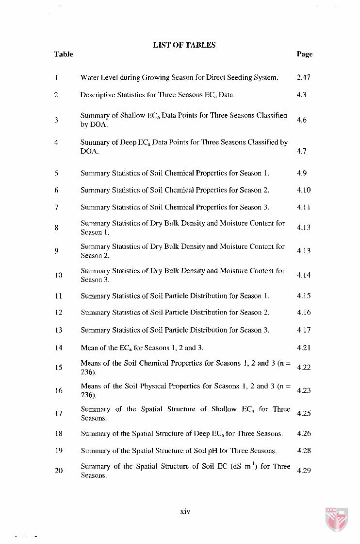
LIST OF TABLES Table Page

Water Level during Growing Season for Direct Seeding System.

Descriptive Statistics for Three Seasons EC, Data.

Summary of Shallow EC, Data Points for Three Seasons Classified by DOA.

Summary of Deep EC, Data Points for Three Seasons Classified by DOA. 4.7

Summary Statistics of Soil Chemical Properties for Season 1.

Summary Statistics of Soil Chemical Properties for Season 2.

Summary Statistics of Soil Chemical Properties for Season 3.

Summary Statistics of Dry Bulk Density and Moisture Content for Season 1 .

Summary Statistics of Dry Bulk Density and Moisture Content for Season 2.

Summary Statistics of Dry Bulk Density and Moisture Content for Season 3.

Summary Statistics of Soil Particle Distribution for Season 1.

Summary Statistics of Soil Particle Distribution for Season 2.

Summary Statistics of Soil Particle Distribution for Season 3.

Mean of the EC, for Seasons 1,2 and 3.

Means of the Soil Chemical Properties for Seasons 1 , 2 and 3 (n = 4.22 236).

Means of the Soil Physical Properties for Seasons 1, 2 and 3 (n = 236).

4.23

Summary of the Spatial Structure of Shallow EC, for Three 4.25 Seasons.

Summary of the Spatial Structure of Deep EC, for Three Seasons.

Summary of the Spatial Structure of Soil pH for Three Seasons.

Summary of the Spatial Structure of Soil EC (dS m-') for Three 4.29 Seasons.

xiv

Summary of the Spatial Structure of Soil OM (%) for Three 4.3 1 Seasons.

22 Summary of the Spatial Structure of OC (%) for Three Seasons.

23 Summary of the Spatial Structure of Total S (%) for Three Seasons. 4.33

Summary of the Spatial Structure of Total N (%) for Three Seasons. 4.35

Summary of the Spatial Structure of Available P (ppm) for Three 4.36 Seasons.

Summary of the Spatial Structure of CEC (cmol, kgv') for Three 4.37 Seasons.

Summary of the Spatial Structure of Ca (cmol, kg-') for Three 4.39 Seasons.

Summary of the Spatial Structure of Mg (cmol, kg-') for Three 4.40 Seasons.

Summary of the Spatial Structure of K (cmol, kg-') for Three 4.4 1 Seasons.

Summary of the Spatial Structure of Na (cmol, kg-') for Three 4.42 Seasons.

Summary of the Spatial Structure of A1 (cmol, kg-') for Three 4.44 Seasons.

Summary of the Spatial Structure of Fe (cmol, kg-') for Three 4.45 Seasons.

Summary of the Spatial Structure of Total Cation (cmol, kg-') for 4.46 Three Seasons.

Summary of the Spatial Structure of BS (%) for Three Seasons. 4.48

Summary of the Spatial Structure of ESP (%) for Three Seasons.

Summary of the Spatial Structure of Dry Bulk Density (g ~ m - ~ ) for Three Seasons.

4.5 1

Summary of the Spatial Structure of Moisture Content (%) for Three Seasons.

4.5 1

Summary of the Spatial Structure of Clay (%) for Three Seasons.

Summary of the Spatial Structure of Silt (%) for Three Seasons.

Summary of the Spatial Structure of Fine Sand (%) for Three 4.57 Seasons.

Summary of the Spatial Structure of Coarse Sand (70) for Three Seasons.

Summary of the Spatial Structure of Sand (%) for Three Seasons.

Summary of Kriged Shallow EC, Maps for Three Seasons Classified by Standard DOA Rank.

Summary of Kriged Deep EC, Maps for Three Seasons Classified by Standard DOA Rank.

Summary of Kriged Shallow EC, Maps for Three Seasons Classified by Smart Quantiles.

Summary of Kriged Deep EC, Maps for Three Seasons Classified by Smart Quantiles.

Summary of Kriged pH Maps for Three Seasons Classified by DOA Recommendation.

Summary of Kriged pH Maps for Three Seasons Classified by Smart Quantiles.

Summary of Kriged EC Maps for Three Seasons Classified by Smart Quantiles.

Summary of the Third Kriged EC Map Classified by Smart Quantiles based on Seasonal Values.

Summary of Kriged OM Maps for Three Seasons Classified by Smart Quantiles.

Summary of Kriged OC Maps for Three Seasons Classified by Smart Quantiles.

Summary of Kriged Total S Maps for Three Seasons Classified by Smart Quantiles.

Summary of Kriged Total N Maps for Three Seasons Classified by Smart Quantiles.

Summary of Kriged Avai. P Maps for Three Seasons Classified by Smart Quantiles.

Summary of Kriged CEC Maps for Three Seasons Classified by Smart Quantiles.

Summary of Kriged Ca Maps for Three Seasons Classified by Smart Quantiles.

Summary of Kriged Mg Maps for Three Seasons Classified by Smart Quantiles.

Summary of Kriged K Maps for Three Seasons Classified by Smart Quantiles.

xvi

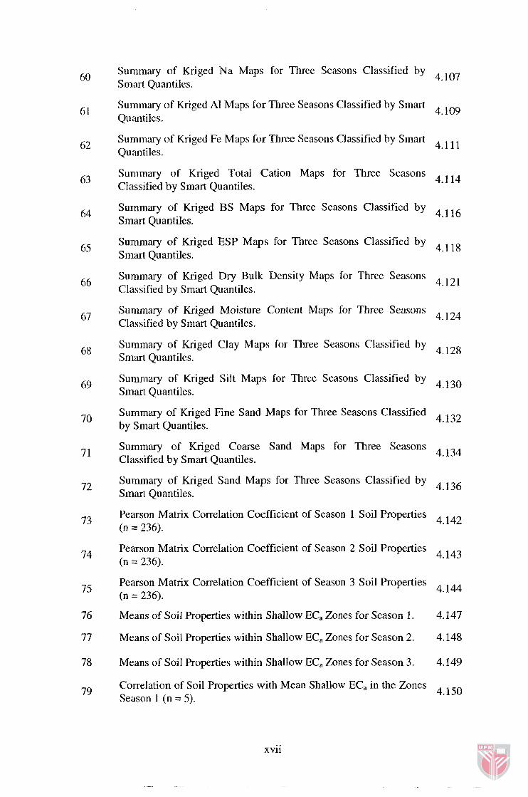
Summary of Kriged Na Maps for Three Seasons Classified by 4.107 60 Smart Quantiles.

Summary of Kriged A1 Maps for Three Seasons Classified by Smart 4.109 Quantiles.

62 Summary of Kriged Fe Maps for Three Seasons Classified by Smart 4.111 Quantiles.

Summary of Kriged Total Cation Maps for Three Seasons 4.1 14 63 Classified by Smart Quantiles.

Summary of Kriged BS Maps for Three Seasons Classified by 4.1 16 Smart Quantiles.

Summary of Kriged ESP Maps for Three Seasons Classified by 4.1 18 Smart Quantiles.

Summary of Kriged Dry Bulk Density Maps for Three Seasons 4.121 Classified by Smart Quantiles.

Summary of Kriged Moisture Content Maps for Three Seasons Classified by Smart Quantiles.

4.1 24

Summary of Kriged Clay Maps for Three Seasons Classified by 4.128 Smart Quantiles.

Summary of Kriged Silt Maps for Three Seasons Classified by 4.130 Smart Quantiles.

Summary of Kriged Fine Sand Maps for Three Seasons Classified 4.1 32 by Smart Quantiles.

Summary of Kriged Coarse Sand Maps for Three Seasons Classified by Smart Quantiles.

4.134

Summary of Kriged Sand Maps for Three Seasons Classified by 4.136 Smart Quantiles.

Pearson Matrix Correlation Coefficient of Season 1 Soil Properties 4.142 (n = 236).

Pearson Matrix Correlation Coefficient of Season 2 Soil Properties 4.143 (n = 236).

Pearson Matrix Correlation Coefficient of Season 3 Soil Properties 4.144 (n = 236).

Means of Soil Properties within Shallow EC, Zones for Season 1

Means of Soil Properties within Shallow EC, Zones for Season 2.

Means of Soil Properties within Shallow EC, Zones for Season 3.

Correlation of Soil Properties with Mean Shallow EC, in the Zones 4.150 Season 1 (n = 5).

xvii

Correlation of Soil Properties with Mean Shallow EC, in the Zones 4.151 Season 2 (n = 5).

Correlation of Soil Properties with Mean Shallow EC, in the Zones 4.152 Season 3 (n = 5).

Means of Soil Properties within Deep EC, Zones for Season 1.

Mean of Soil Properties within Deep EC, Zones for Season 2.

Mean of Soil Properties within Deep EC, Zones for Season 3.

Correlation of Soil Properties with Mean Deep EC, in the Zones for Season 1 (n = 5).

4.158

Correlation of Soil Properties with Mean Deep EC, in the Zones for 4-159 Season 2 (n = 5).

Correlation of Soil Properties with Mean Deep EC, in the Zones for Season 3 (n = 5).

4.160

Significant Curve Fit Estimation Model for Soil Chemical 4.162 Properties in the Entire Study Area (n = 236).

Significant Curve Fit Estimation Model for Soil Physical Properties in the Entire Study Area (n = 236).

4.163

The Best Curve Estimation for Soil Properties and Shallow EC, 4.165 (n=5).

The Best Curve Estimation for Soil Properties and Deep EC, (n=5). 4.166

The Best Curve Estimation for Soil Properties and Shallow EC, in Zone 1 Shallow EC, for Three Seasons.

4.1 67

The Best Curve Estimation for Soil Properties and Shallow EC, in 4.169 Zone 2 Shallow EC, for Three Seasons.

The Best Curve Estimation for Soil Properties and Shallow EC, in 4.170 Zone 3 Shallow EC, for Three Seasons.

The Best Curve Estimation for Soil Properties and Shallow EC, in Zone 4 Shallow EC, for Three Seasons.

4.171

The Best Curve Estimation for Soil Properties and Shallow EC, in 4.171 Zone 5 Shallow EC, for Three Seasons.

The Best Curve Estimation for Soil Properties and Deep EC, in Zone 1 Deep EC, for Three Seasons.

4.173

The Best Curve Estimation for Soil Properties and Deep EC, in 4.174 Zone 2 Deep EC, for Three Seasons.

The Best Curve Estimation for Soil Properties and Deep EC, in Zone 3 Deep EC, for Three Seasons.

4.175

xviii

The Best Curve Estimation for Soil Properties and Deep EC, in 4.176 Zone 4 Deep EC, for Three Seasons.

The Best Curve Estimation for Soil Properties and Deep EC, in Zone 5 Deep EC, for Three Seasons.

4.177

Summary of Three Season Yields for 1 18 Plots.

xix

LIST OF FIGURES

Figure Page

The System Components of Veris Soil EC Mapping-Model: Veris3 100.

Schematic of Electrodes Configuration (a) Shallow and, (b) Deep Readings.

Contour Plots of the Measured Signal by Each Unit Soil Volume (Boydell et al., 2003).

2.5

GPS Satellite Constellation.

GPS Satellite.

GPS Signal Structure.

Control Segment Station Locations.

GPS User Segment.

Intersection of Three Imaginary Spheres.

Four Required Satellites to Obtain a Position and Time in 3 Dimensions.

Pseudo Random Code.

Steps of Precision Farming.

Concept of Accuracy and Precision.

A Typical Variogram Model.

Typical Ideal Water Management in Rice Cultivation (FAO, 1989). 2.48

Sawah Sempadan Compartment and Block C (a) Satellite Image for Tanjong Karang Rice Irrigation Scheme, (b) Satellite Image for Sawah Sempadan Rice Irrigation Compartment, and (c) Block C at

3.2

Sawah Sempadan Rice Irrigation Compartment.

Soil Series Map of Block C, Sawah Sempadan (DOA, 2000).

VerisEC 3 100 with DGPS was Pulled by a Tractor in a Paddy Field (a) 35HP Tractor was used in Season 1 and, (b) 80HP Tractor was used in the following Two Seasons.

Schematic of Study Steps.

The Distribution of Shallow EC, (mS m-') Values within the Study 4-4 Area (a) Season 1, (b) Season 2, and (c) Season 3.

The Distribution of Deep EC, (mS m-I) Values within the Study Area 4.5 (a) Season 1, (b) Season 2, and (c) Season 3.

Typical Map of the Soil Chemical and Physical Sampling Points in 4-8 Block C for Three Seasons.

Season 1 Soil Texture Distributed on Triangular Class.

Season 2 Soil Texture Distributed on Triangular Class.

Season 3 Soil Texture Distributed on Triangular Class.

lsotrophic Variograms of Shallow EC, (mS m-I).

Isotrophic Variograms of Deep EC, (mS m-I).

Isotrophic Variograms of Soil pH.

Isotrophic Variograms of Soil EC (dS m-').

Isotrophic Variograms of Soil OM (%).

Isotrophic Variograms of OC (%).

Isotrophic Variograms of Total S (%).

Isotrophic Variograms of Total N (%).

Isotrophic Variograms of Available P (ppm).

lsotrophic Variograms of CEC (cmol, kg-').

Isotrophic Variograms of Ca (cmol, kg-').

Isotrophic Variograms of Mg (cmol, kg-').

xxi

Isotrophic Variograms of K ( ~ m o l , ~ . ~ kg-').

lsotrophic Variograms of Na (cmol, kg-').

Isotrophic Variograms of A1 (cmol, kg-').

Isotrophic Variograms of Fe (cmol, kg-').

Isotrophic Variograms of Total Cation (cmol, kg-').

Isotrophic Variograms of BS (%).

Isotrophic Variograms of ESP (%).

Isotrophic Variograms of Dry Bulk Density (g cm-').

Isotrophic Variograms of Moisture Content (%).

Isotrophic Variograms of Clay (%).

Isotrophic Variograms of Silt (%).

Isotrophic Variograms of Fine Sand (%).

Isotrophic Variograms of Coarse Sand (%).

Isotrophic Variograms of Sand (%).

Kriged Map for Shallow EC, (mS m-I) Classified by Standard DOA 4.62 EC Rank (a) Season 1, (b) Season 2, and (c) Season 3.

Kriged Map for Deep EC, (mS m-') Classified by Standard DOA EC 4.63 Rank (a) Season 1, (b) Season 2, and (c) Season 3.

Kriged Map for Shallow EC, (mS m-I) Classified by Smart Quantiles 4.67 (a) Season 1, (b) Season 2, and (c) Season 3.

Kriged Map for Deep EC, (mS m-I) Classified by Smart Quantiles (a) 4.70 Season 1, (b) Season 2, (c) Season 3, and (d) Soil Series Map.

Kriged Map for pH Classified by DOA (a) Season 1, (b) Season 2, 4.73 and (c) Season 3.

xxii

Kriged Map for pH Classified by Smart Quantiles (a) Season 1, (b) 4.76 Season 2, and (c) Season 3.

Kriged Map for EC (dS m-I) Classified by Smart Quantiles (a) 4+79 Season 1, (b) Season 2, and (c) Season 3.

Kriged Map for OM (%) Classified by Smart Quantiles (a) Season 1, 4.82 (b) Season 2, and (c) Season 3.

Kriged Map for OC (%) Classified by Smart Quantiles (a) Season 1, (b) Season 2, and (c) Season 3.

4.84

Kriged Map for Total S (%) Classified by Smart Quantiles (a) Season 4.87 1, (b) Season 2, and (c) Season 3.

Kriged Map for Total N (%) Classified by Smart Quantiles (a) 4.90 Season 1, (b) Season 2, and (c) Season 3.

Kriged Map for Avai. P (ppm) Classified by Smart Quantiles (a) Season 1, (b) Season 2, and (c) Season 3 Classified to Seasonal Smart 4.93 Quantiles.

Kriged Map for CEC (cmol, kg-') Classified by Smart Quantiles (a) 4.96 Season 1, (b) Season 2, and (c) Season 3.

Kriged Map for Ca (cmol, kg-') Classified by Smart Quantiles (a) Season I , (b) Season 2, and (c) Season 3.

4.99

Kriged Map for Mg (cmol, kg-') Classified by Smart Quantiles (a) 4.102 Season 1, (b) Season 2, and (c) Season 3.

Kriged Map for K (crnol, kg') Classified by Smart Quantiles (a) 4.105 Season 1, (b) Season 2, and (c) Season 3.

Kriged Map for Na (cmol, kg-') Classified by Smart Quantiles (a) 4.108 Season 1, (b) Season 2, and (c) Season 3.

Kriged Map for A1 (cmol, kg-') Classified by Smart Quantiles (a) 4.1 Season 1, (b) Season 2, and (c) Season 3.

Kriged Map for Fe (cmol, kg-') Classified by Smart Quantiles (a) 4.112 Season 1, (b) Season 2, and (c) Season 3.

Kriged Map for Total Cation (cmol, kg ') Classified by Smart 4.115 Quantiles (a) Season 1, (b) Season 2, and (c) Season 3.

Kriged Map for BS (%) Classified by Smart Quantiles (a) Season 1, 4. l7 (b) Season 2, and (c) Season 3.

Kriged Map for ESP (%) Classified by Smart Quantiles (a) Season 1, 4. (b) Season 2, and (c) Season 3.

Kriged Map for Dry Bulk Density (g cm") Classified by Smart 4.122 Quantiles (a) Season 1, (b) Season 2, and (c) Season 3.

Kriged Map for Moisture Content (96) Classified by Smart Quantiles 4.125 (a) Season 1, (b) Season 2, and (c) Season 3.

xxiii

Kriged Map for Clay (%) Classified by Smart Quantiles (a) Season 1, (b) Season 2, and (c) Season 3.

4.129

Kriged Map for Silt (%) Classified by Smart Quantiles (a) Season I, 4.131 (b) Season 2, and (c) Season 3.

Kriged Map for Fine Sand (%) Classified by Smart Quantiles (a) 4.133 Season 1, (b) Season 2, and (c) Season 3.

Kriged Map for Coarse Sand (%) Classified by Smart Quantiles (a) 4.135 Season 1, (b) Season 2, and (c) Season 3.

Kriged Map for Sand (%) Classified by Smart Quantiles (a) Season 1, 4. 37 (b) Season 2, and (c) Season 3.

Thematic Maps for Yield (kg ha-') (a) Season I , (b) Season 2, and (c) 4.187 Season 3.

Relationship between Yield (kg ha-') and Shallow EC, (mS m-') for 4.189 all the Seasons.

Relationship between Yield (kg ha.') and Deep EC, (mS m-') for all 4.189 the Seasons.

xxiv