Embed Size (px)
Citation preview

Registered under N°: 4502-16/UAC/VR-AARU/SA
A DISSERTATION
Submitted
In partial fulfillment of the requirements for the degree of
DOCTOR of Philosophy (PhD) of the University of Abomey-Calavi (Benin Republic)
In the framework of the
Graduate Research Program on Climate Change and Water Resources (GRP-CCWR)
By
Jamilatou Chaibou Begou
Public defense on: 26/10/2016
======
Hydrological Modeling of the Bani Basin in West Africa:
Uncertainties and Parameters Regionalization ======
Supervisors:
Abel Afouda, Professor, UAC (Benin) Michael Rode, PD Dr., UFZ (Germany) Sihem Benabdallah, Professor, CERTE (Tunisia)
======
JURY
Boukari Moussa Professor, UAC (Benin) President
Lawin Emmanuel Associate Professor, UAC (Benin) Reporter
Rabani Adamou Associate Professor, UAM (Niger) Reporter
Julien Adounkpe Associate Professor, UAC (Benin) Examiner
Abel Afouda Professor, UAC (Benin) Supervisor
UNIVERSITE D’ABOMEY - CALAVI (UAC) INSTITUT NATIONAL DE L’EAU
West African Science Service Center on Climate
Change and Adapted Land Use

i
Dedication
To my precious son, Ismail of whom I was gifted during my PhD. I did not
often have enough time for you, you endured my long absences but you gave
me courage and motivation. It was not easy but I did it for you!

ii
Acknowledgments
The objectives of this research project would not have been met without the support of several
institutions and people.
First, I would like to thank profusely the German Ministry of Education and Research (BMBF) for
financing my PhD through the West African Science Service Centre on Climate Change and
Adapted Land Use (WASCAL; www.wascal.org) that supports the Graduate Research Program
Climate Change and Water Resources at the University of Abomey-Calavi. I would like also to
thank AGRHYMET Regional Centre for providing additional funds to this PhD through the French
Global Environment Facility (FFEM/CC) project.
I would like to express here my gratitude to all my collaborators for many interesting comments
and suggestions as well as for the encouragement I have received during my Thesis in connection
with the experiments, the data analysis and the model application.
First, I would like to thank my supervisor, Professor Abel Afouda, the Director of the WASCAL
Graduate Research Program on Climate Change and Water Resources at the University of
Abomey-Calavi. His strong encouragement, support and especially his endless patience in
discussing the results and improving my writing have helped foster the achievement of this thesis.
I especially want to thank my PhD co-supervisors PD Michael Rode and Professor Sihem
Benabdallah for providing me with interesting discussions, which have clearly improved my
scientific approach. The three scientific stays I have carried out at your research institutions
(CERTE, Tunisia and UFZ, Germany), the expertise on the SWAT model I received, the continual
help on improving results and writing the dissertation till the end, have surely played a crucial role
on the success of this work.
I will be forever grateful to Dr. Seifeddine Jomaa, Postdoctoral researcher at UFZ (Germany). The
first words that come to my mind are “you helped me find my way!” From the valuable scientific
discussions we had at conferences, at UFZ and through the network, the guidance in the vast world
of a PhD student, the help to win a grant from the prestigious European Geosciences Union (EGU)
and to participate to its Assembly, the interminable help in writing, I run out of alphabet! More,
you marked our scientific collaboration with human values that made us “just a family”
I am also extremely grateful to Dr. Pignina Bazie, Coordinator of the French Global Environment
Facility (FFEM/CC) project executed by AGRHYMET. You provided me with administrative and
financial supports at AGRHYMET and many scientific discussions on the hydrogeological aspects
of river basin modeling. Thank you for your endless assistance since my engineering degree.
To all the staff of WASCAL Graduate Research Program on Climate Change and Water Resources
(GRP-CCWR) hosted by the University of Abomey-Calavi (UAC), find here my sincere gratitude!
I am extremely grateful to AGRHYMET and Namodji Lucie, the climatological database manager,
for providing climatic data. I would like also to thank the National Hydrological Service of Mali,
through the intermediary of Traore Chaka and Mama Yena, for discharge data, Kone Soungalo for
climate data on the Ivorian part of the Bani basin and Francois Laurent for soil and land use
databases.

iii
I would like to thank Dr. Aissata Boubacar for her trustworthy encouragements that I drew from
the interminable academic discussions we had and experience we shared, Issa Saley for the course
on statistics, hands on R statistical software and data pre-processing.
Last, but not the least, I would like to thank profusely my family, especially my parents who always
support me, wishing me always the best, my mother taking care of my son whenever I was away,
even following me during my scientific stay in Tunisia, my husband Dr. Yacouba and my lovely
son Ismail for their patience in my long absences: in Ghana, Benin, Tunisia, Germany,
Netherlands, Austria, and my sister Maimouna for relieving my mother near my son. You are the
source where I draw daily energy! Thanks forever!
To everyone who brings whatever support, be it directly or indirectly to this work, find here my
sincere gratitude!

iv
Abstract
In many drainage basins around the world, no runoff data are available. This situation is more
pronounced in developing countries, where many river basins lack runoff data and so are
ungauged. In West Africa, the general situation of insufficient data is exacerbated by the decline
of the measuring network observed since the late eighties. With the aim of predicting hydrological
variables in ungauged basins, regionalization methods are usually used. The main objective of this
study is to make prediction of streamflow hydrographs on the Bani basin to improve the knowledge
of water resources availability. Firstly, the hydrological model SWAT was calibrated on many
gauged catchments on the period 1983-1992 and validated on 1993-1997 using the Generalized
Likelihood Uncertainty Estimation (GLUE) approach. Secondly, the studied catchments were
categorized into clusters of similar physioclimatic characteristics by the means of a multivariate
statistical analysis. And finally, in each case, the entire set of optimized model parameters was
transferred from gauged to ungauged catchments based on physical similarity and spatial
proximity approaches, and the discharge hydrograph was simulated on the target catchment for the
period 1983-1997. Results indicated that the daily model performs as good as the monthly model
at catchment and subcatchment scales, despite the limited data condition underlying the
hydrological modeling. On a daily basis, a good performance of the SWAT model at the whole
catchment scale has been obtained as depicted by a Nash-Sutcliffe Efficiency (NSE) of 0.76 and
0.84 and a coefficient of determination R2 of 0.79 and 0.87 for calibration and validation periods,
respectively. In addition, the PBIAIS values were smaller than 25% in magnitude for both
calibration and validation periods, reflecting a reasonable prediction of the water balance.
Predictive uncertainties were acceptable despite being larger during high and low flows conditions.
The 61% of observed data (P-factor = 0.61) were enclosed within a small uncertainty band (R-
factor = 0.91). A better model performance and smaller predictive uncertainties have been
achieved with monthly calibration compared to daily calibration, except for the water balance,
where errors have slightly increased. A total of 12 model parameters were identified that best
simulate the observed discharges. The test catchments principally aggregated into three groups: a
group of northerly flat and semi-arid catchments, another group of southerly hilly and humid
catchments, and a third group located in the center of the study basin, inside which, none of the
descriptors seems to exert a strong control on the similarity. Overall, regionalization yielded

v
satisfactory to very good results at many target catchments. The best efficiencies have been
recorded in the arid zone and at the whole catchment outlet with NSE values ranging between 0.56
and 0.83. However, predictive uncertainty showed an increase with aridity. A good mutual
hydrological similarity was found in a set of catchments belonging to different physical regions,
and between which, spatial proximity was found to be a better surrogate of this similarity. The
knowledge of water resources availability where it is not measured is very useful for many
applications such as water allocation for consumption and irrigation especially in West Africa
frequently facing water deficit and food insecurity due to the impacts of a changing climate.
Results also contribute to the advance in understanding of hydrological processes of a newly
investigated area in the field of Prediction in Ungauged Basins (PUB), and constitute a first step
toward further investigations on catchment functioning on which depends largely the success of
any regionalization of hydrological information.
Keywords: Prediction in ungauged Basins, SWAT model parameters, Performance and predictive
uncertainty, Multivariate statistics, Catchments similarity, Regionalization.

vi
Résumé
De nombreux bassins de drainage à travers le monde ne disposent d’aucune mesure de débit. Les
méthodes de régionalisation sont alors généralement utilisées pour les prévisions en bassins non
jaugés. L'objectif principal de cette étude est de prévoir les hydrogrammes d’écoulement dans le
bassin du Bani afin de contribuer à l’amélioration de la connaissance sur la disponibilité des
ressources en eau. Tout d'abord, le modèle hydrologique SWAT a été calibré sur de nombreux
bassins jaugés sur la période de 1983-1992 et validé sur la période 1993-1997 en utilisant la
méthode « Generalized Likelihood Uncertainty Estimation (GLUE) ». Ensuite, des groupes de
bassins similaires ont été déterminés en fonction de leurs caractéristiques physiographiques et
climatiques et au moyen d’une analyse statistique multivariée. Deux méthodes de régionalisation
basées sur le concept de similarité entre bassins, ont été utilisées : la similarité physique et la
proximité spatiale. Dans les deux cas, le jeu de paramètres calés du modèle est entièrement
transféré du bassin jaugé vers le bassin non jaugé pour y simuler l’hydrogramme de débits
journaliers de la période 1983-1997. Les résultats indiquent une bonne performance du modèle à
l’échelle journalière et mensuelle, ainsi qu’à l’échelle du bassin et des sous-basins. La performance
du modèle à l’échelle du bassin global et sur un pas de temps journalier est caractérisée par un
critère de Nash de 0.76 et 0.84 et un coefficient de détermination de R2 de 0.79 et 0.87 en période
de calibration et de validation, respectivement. Aussi, les valeurs absolues du PBIAIS demeurent
inferieures à 25%, ce qui témoigne d’une bonne prévision du bilan d’eau. Il est à noter que les
incertitudes associées demeurent satisfaisantes malgré les conditions de données limitées qui sous-
tendent cette modélisation. Ainsi, 61% des débits observés (P-factor = 0.61) sont compris à
l’intérieur de la bande d’incertitude dont la largeur reste adéquate (R-factor = 0.91). La calibration
mensuelle a quant à elle permit d’atteindre une meilleure performance du modèle et une diminution
des incertitudes à l’exception du bilan d’eau dont les erreurs de prévision semblent avoir augmenté.
La calibration a également permis d'identifier 12 paramètres du modèle qui simulent au mieux les
débits observés. Les bassins étudiés ont été classes en trois groupes: un groupe de bassins de plaine,
semi-arides et situés au Nord, un autre groupe de bassins d’altitude qu’on rencontre dans les zones
humides du Sud, et un troisième groupe situé dans le centre du bassin d'étude, à l'intérieur duquel,
aucun des descripteurs semble se démarquer significativement des autres. Dans l'ensemble, la
régionalisation a donné de bons résultats au niveau de plusieurs bassins cibles. Les meilleurs ont

vii
toutefois été enregistrés dans la zone aride et à l’exutoire global du bassin, particulièrement.
Cependant, on note également une augmentation des incertitudes précisément dans cette zone. Une
bonne similarité hydrologique mutuelle a été mise en évidence entre certains bassins, dont le
meilleur indicateur reste la proximité spatiale. La connaissance de la disponibilité des ressources
en eaux, particulièrement au niveau des bassins non jauges, est d’une utilité capitale dans plusieurs
domaines d’application telles que l'allocation de l'eau pour la consommation et pour l'irrigation
surtout en Afrique de l'Ouest qui fait face fréquemment à la gestion des risques liés au déficit en
eau et a l'insécurité alimentaire en raison des impacts du changement climatique. Ces résultats
contribuent également à une meilleure compréhension du fonctionnement hydrologique d’une
zone jusque-là non explorée dans le domaine de la prévision en bassins non jaugés (PUB), et
constituent une première étape vers de nouvelles investigations qui contribueront à l’amélioration
des prévisions de l’information hydrologique.
Mots clés : Prévisions en Bassins non jaugés, Paramètres du modèle SWAT, Performance et
incertitudes liées à la prévision, Analyse multivariée, Similarité entre bassins, Régionalisation.

viii
Table of Contents
Dedication .................................................................................................................. i
Acknowledgments ..................................................................................................... ii
Abstract .................................................................................................................... iv
Résumé ..................................................................................................................... vi
Table of Contents ................................................................................................... viii
List of Tables ............................................................................................................. x
List of Figures .......................................................................................................... xi
1. Introduction ........................................................................................................... 2
1.1. Problem statement ................................................................................................................ 2
1.2. Scope of the study ................................................................................................................ 3 1.3. Outline of the Thesis ............................................................................................................ 6
2. Literature review ................................................................................................... 8
2.1. Hydrological modeling of the Bani basin ............................................................................ 8
2.2. Catchment classification and similarity frameworks ......................................................... 12 2.3. Regionalization approach for flow prediction in ungauged basins .................................... 14
3. Material and Methods .........................................................................................19
3.1. The study catchment .......................................................................................................... 19 3.2. Calibration and validation of the SWAT model ................................................................ 21 3.2.1. Model description ....................................................................................................................... 21 3.2.2. Input data and databases ............................................................................................................. 23 3.2.3. Hydro-meteorological data and quality control .......................................................................... 24 3.2.4. GIS-data and databases ............................................................................................................... 29 3.2.5. Pre-processing of the SWAT input data for the Bani catchment ................................................ 31 3.2.6. Model setup ................................................................................................................................. 35 3.2.7. Calibration and validation procedures ........................................................................................ 36 3.2.8. Model performance and uncertainty evaluation .......................................................................... 38 3.2.9. Sensitivity analysis ...................................................................................................................... 39 3.2.10. Verification of model outputs ................................................................................................. 39
3.3. Catchments classification .................................................................................................. 40 3.3.1. Catchments and catchments’ attributes ....................................................................................... 41 3.3.2. Multivariate statistical analyses .................................................................................................. 44
3.4. Model Parameters Regionalization .................................................................................... 48 3.4.1. Study catchments and modeling framework ............................................................................... 48 3.4.2. Regionalization approaches and similarity frameworks ............................................................. 50 3.4.3. Evaluation of the regionalization performance and prediction uncertainty ................................ 51

ix
3.4.4. Assessment of the hydrological similarity .................................................................................. 52
4. Results and Discussions ......................................................................................54
4.1. Multi-site Validation of the SWAT Model on the Bani Catchment: Model Performance
and Predictive Uncertainty* .......................................................................................................... 54 4.1.1. The catchment scale model ......................................................................................................... 55 4.1.2. The subcatchment model ............................................................................................................ 61 4.1.3. Discussion and conclusions ........................................................................................................ 63
4.2. Catchment Classification: Multivariate Statistical Analysis for Physiographic Similarity*
69 4.2.1. Catchments clustering ................................................................................................................. 70 4.2.2. Major controlling factors of similarity ........................................................................................ 73 4.2.3. Discussion and conclusions ........................................................................................................ 76
4.3. Predicting Daily Discharge Hydrograph in Ungauged Basins Based on Similarity
Approach ....................................................................................................................................... 79 4.3.1. Calibration at gauged catchments ............................................................................................... 80 4.3.2. Prediction of discharge hydrographs in ungauged basins ........................................................... 82 4.3.3. Discussion and conclusions ........................................................................................................ 90
5. Conclusions and Perspectives .............................................................................98
5.1. Conclusions ........................................................................................................................ 98 5.2. Perspectives and recommendations ................................................................................. 100
References ..............................................................................................................102
Appendices .............................................................................................................112
Appendix A: Published article 1 ................................................................................................. 112 Appendix B: Published article 2 ................................................................................................. 112

x
List of Tables
Table 2-1. Summary of the previous hydrological modeling studies conducted on the Bani basin. ................. 10
Table 3-1. Input data of the SWAT model for the Bani catchment. .................................................................. 23
Table 3-2. Available daily precipitation data time series: length and completeness. ........................................ 25
Table 3-3. Available discharge measurements on the Bani. .............................................................................. 28
Table 3-4. Description of the SWAT land use classes of the Bani catchment. ................................................. 32
Table 3-5. Description of SWAT soil classes of the Bani catchment. .............................................................. 34
Table 3-6. Precipitation gauge location table. ................................................................................................... 34
Table 3-7. Input methods for SWAT model simulation on the Bani catchment. .............................................. 35
Table 3-8. Summary of catchment attributes derived by the SWAT model as input for multivariate statistical
analysis on the Bani catchment. .................................................................................................................. 43
Table 3-9. Description of candidate catchments for model parameters regionalization. .................................. 49
Table 4-1. Model performance statistics and predictive uncertainty indices of the SWAT model for the Bani
catchment at Douna, Pankourou and Bougouni discharge gauging stations............................................... 56
Table 4-2. Average annual basin values of precipitation (P), Evapotranspiration (ET), Potential
Evapotranspiration (PET) and biomass as SWAT outputs on the Bani catchment. ................................... 58
Table 4-3. Sensitivity of the calibrated SWAT model parameters on the Bani catchment at Douna on a daily
time interval. ............................................................................................................................................... 59
Table 4-4. Description of hierachical clusters. In bold, positive v-test values indicate the variable that has a
value greater than the overall mean, and in italic, negative v-test values refer to the variable that has a
value smaller than the overall mean. All v-test values are significant at the probability p = 0.05. ........... 74
Table 4-5. Performance statistics and prediction uncertainty indices of the SWAT model for the Bani
catchment. In bold, NSE values greater than 0.5, and PBIAIS less than ±25% in absolute values. ............ 81
Table 4-6. Performance of the SWAT model parameters transfer inside the Bani catchment. In bold, above-
threshold statistics of a satisfactory regionalization, while in italic below-threshold statistics. ................. 82
Table 4-7. Ratio between regionalization performance and calibration performance at target catchment. ...... 88

xi
List of Figures
Figure 3-1. Localization of the Bani catchment and the hydro-climatic monitoring network. ......................... 21
Figure 3-2. Examples of quality control test failures (a) Inconsistency in daily temperature data at Segou (b)
implausible minimum temperature values at Bougouni. ............................................................................. 27
Figure 3-3. Land use/land cover maps of the Bani (a) original GLCC land cover and (b) SWAT land use
classes after reclassification. ....................................................................................................................... 32
Figure 3-4. Soil maps of the Bani (a) original FAO soils and (b) SWAT soil classes after reclassification. .... 33
Figure 3-5. Study catchments and Digital Elevation Model of the Bani basin. ................................................ 42
Figure 3-6. Localization of the test catchments for model parameters transfer on the Bani basin. ................... 49
Figure 4-1. Simulated and observed hydrographs at Douna station at (a) daily and (b) monthly timesteps along
with calculated statistics on calibration and validation periods. ................................................................. 57
Figure 4-2. Spatial validation of the SWAT model on the Bani catchment. The model was turned at
Pankourou ((a) daily and (b) monthly timesteps) and at Bougouni ((c) daily and (d) monthly timesteps) by
using the same behavioral parameter sets determined at the Douna outlet on the period 1983-1992. ....... 60
Figure 4-3. Simulated and Observed hydrographs at Pankourou station at (a) daily and (b) monthly timesteps
along with calculated statistics on calibration and validation periods. ....................................................... 62
Figure 4-4. Predicted and measured discharges at Bougouni station at (a) daily and (b) monthly intervals
during the calibration and validation periods with their corresponding statistics. ...................................... 62
Figure 4-5. Hierarchical clustering representation on the map induced by the first 2 Principal Components on
the Bani catchment. Sub-catchments are coloured according to the cluster they belong to, the barycenter
of each cluster is represented by a square and Dim1 and Dim2 are the first two Principal Components on
which the hierarchical clustering is built. ................................................................................................... 71
Figure 4-6. Hierarchical dendrogram of the Bani catchment. Each rectangle represents a cluster of similar
catchments. The barplot (inertia gain) gives the decrease of within-group variability with increasing
number of clusters. ...................................................................................................................................... 73
Figure 4-7. The spatial distribution of clusters of physically similar catchments on the Bani basin ................ 76
Figure 4-8. Prediction uncertainty band of model parameters transfer at ungauged catchments (in gray)
represented by R-factor values. In blue, initial uncertainty band at the donor catchment. ......................... 84
Figure 4-9. Measured and predicted discharge on the target catchments (Douna (a)-(b), Debete (c)-(d), Dioila
(e)-(f) and Pankourou (g)-(h)) using different donor catchments. Note that the title of each subplot (for
example Douna (Dioila) in subplot (a)) means Target (Donor) catchment, respectively. .......................... 87
Figure 4-10. Spatial pattern of the discharge hydrograph regionalization. The number of symbols inside each
catchment represents the number of simulation with NSE greater than 0.5. The aridity index was
calculated on the period 1983-1998. ........................................................................................................... 89

Page 1
CHAPTER I

Page 2
1. Introduction
1.1. Problem statement
Water resources managers are facing challenges in many river basins across the world due to
limited data availability. Climate and land use changes – be it natural or human-induced – add
more complexity to this task (Pomeroy et al., 2013; Sivapalan et al., 2003). This situation is
more pronounced in developing countries, where in many river basins no runoff data is
available (Bormann and Diekkrüger, 2003; Kapangaziwiri et al., 2012; Mazvimavi et al., 2005;
Minihane, 2013; Ndomba et al., 2008) and the existing ones are of questionable quality or at
best short or incomplete.
The Niger River basin is not an exception to that fact. In the eighties and nineties, for instance,
hydrometric stations were reduced to a minimum (Nkamdjou and Bedimo (2008)). To prevent
the hydrologic observing system from more degradation, the Niger Basin Authority (NBA) has
set the Niger-HYCOS project, which one of its specific objectives is to improve data quality
of the Niger River. For this purpose, the project identified and brings assistance in the
installation and the management of 105 hydrometric stations shared by nine countries drained
by the River, and contributes to the capacity building of national hydrological services.
In its fifth assessment report on regional aspects of climate change, the Inter-Governmental
Panel on Climate Change (IPCC, 2014) has shown that adaptation to climate change in Africa
is confronted with a number of challenges among which is a significant data gap. Too many
basins lack reliable data necessary to assess in details impacts of climate change on different
components of the hydrological cycle and to develop strategies of adaptation related to each
specific impact. Thus, there is an urgent need to predict hydrological variables in ungauged
basins for building high adaptive capacity by improving: (i) water resources knowledge,

Page 3
planning and management, (ii) identification and implementation of strategies of adaptation to
climate change in the sector of water, and (iii) ecological studies for a sustainable development.
Additionally, Blöschl et al. (2013) developed an exhaustive range of applications for which
prediction in ungauged basins is needed, such as hydraulic structures design, flood and drought
management, water allocation, hydropower, ecological purposes and water quality, to cite few.
Another important problem that is now acknowledged by the international community is the
increasing importance of uncertainty analysis in hydrology (Beven, 2008; Hrachowitz et al.,
2013). Hydrological predictions should systematically integrate uncertainty analysis (Beven,
2006) and thus provide not only one situation, but a variety of possible situations on which
decisions can be built (Dessai et al., 2009; Paturel, 2014). As discussed by Hulme (2011).
Decision-makers need uncertainty evaluation rather than pseudo-certainty. Possible future
scenarios are more needed for Prediction in Ungauged Basins (PUB) which adds to the
traditional uncertainty related to hydrological modeling (related to input data, model structural
errors, and parameters identification), another source of uncertainty related to model
parameters transfer. However, little attention has been given to the uncertainty resulting from
model parameters regionalization at ungauged sites (Wagener and Wheater, 2006), especially
on the Bani catchment, where to our knowledge no such a study exists.
1.2. Scope of the study
With the aim of predicting hydrological variables in ungauged basins, regionalization
procedures are usually used. Different types of regionalization methods exist, and can be
divided into (He et al., 2011; Hrachowitz et al., 2013): (1) Regionalization of flow and flow
metrics, and (2) regionalization of model parameters. The latter is a process-based method and
involves the application of a rainfall-runoff model and the transfer of model parameters from
gauged to ungauged catchments. In spite of the additional uncertainties related to input data,

Page 4
model structure, parameter identification, and the need of rigorous calibration at gauged
catchments (Blöschl, 2011; He et al., 2011; Wagener and Wheater, 2006), it remains a long-
standing method (Wagener et al., 2004a) for flow prediction in ungauged basins. Because of
runoff process results from the interaction between all important processes within a catchment,
and these processes can be physical, chemical and biological (Blöschl et al., 2013). The
quantification of the impact of such processes on the runoff behaviour can only be
approximated by a hydrological model. The transfer of model parameters can make use of
either regression-based methods or distance-based methods. The latter group of methods
assumes that there exists a similarity measure, which can be used to transfer, to a certain extent,
hydrological information from a catchment to another to which it is similar.
Given this background, the main objective of this thesis is to make predictions of streamflow
hydrographs on the Bani basin to improve the knowledge of water resources availability. The
specific objectives are to:
Calibrate a rainfall-runoff model on many gauged catchments and identify the best
model parameter sets;
Provide a classification of catchments based on their physiographic and climatic
characteristics
And regionalize the optimized model parameters from gauged to ungauged catchment
based on the physical similarity, and achieve discharge hydrograph without need of any
measurement.
Specific research questions are addressed in order to achieve the aforementioned objectives:
(1) To which extent does the SWAT model for the Bani catchment depend on the temporal and
spatial scale?

Page 5
(2) What are the SWAT model parameters that best describe the hydrological behaviour of the
Bani basin?
(3) Can the use of measured sparse point rain gauge data provide valuable information for
discharge simulation?
(4) What is the physio-climatic pattern of similarity between catchments?
(5) What are the dominant controls on similarity between catchments?
(6) Is there any pattern of the regionalization performance and prediction uncertainty?
(7) Which similarity-based method for regionalization performs best?
(8) Does physical similarity entail hydrological behaviour of a catchment?
By contributing to the advance in regionalization of hydrological information across regions,
this work provides the first ever complete study on discharge hydrograph prediction at
ungauged basins on a data-sparse large Soudano-Sahelian catchment subject to different
climate, soil and land use variabilities. The originality of this work resides in the combined use
of daily and subcatchment performances along with the assessment of prediction uncertainty
to provide finer temporal and spatial hydrological information and its range of variations at
gauged and ungauged sites. Another important output of this work is the involvement of
evapotranspiration (the most important component of the water balance after rainfall especially
under warm climate) in the verification of model outputs reasonability, a particular attention
that has not been considered by any previous study in the region. In addition, we used point
rain gauge data (as per SWAT’s standard procedure) opposed to areal precipitation in order to
maintain the real data condition (limited in time and space) as far as possible.

Page 6
1.3. Outline of the Thesis
To address the aforementioned research questions, the Thesis is organized in 5 Chapters.
Chapter I presents the general introduction of the thesis; the problem that supports the research
is stated and the objectives and research questions are clearly presented.
Chapter II provides a literature review in order to estimate the current knowledge on the
hydrological modeling of the study area, catchments classification and similarity frameworks
and regionalization approach for flow prediction in ungauged basins.
Chapter III is dedicated to the description of the input data and the particular methods involved
in the research process. First, we describe the general modeling framework of the thesis in
which we tried to address the questions (1) to (3). The objectives were to assess the
performance and prediction uncertainty of the SWAT model on daily and monthly time
intervals and at catchment and subcatchment levels, and to identify the model parameters that
best describe the hydrological functioning of the catchment. Second, we shed light on the
similarity framework between catchments by addressing questions (3) and (4). The objectives
were to group catchments into clusters of similar physiographic and climatic characteristics,
and determine the main causes of similarity. Finally, the regionalization approach is explained
that deals with questions (6) to (8). The objectives were to predict daily streamflow hydrograph
at ungauged catchments based on similarity concepts, and assess the prediction uncertainty
related to the model parameters transfer.
Chapter IV presents the main findings, their corresponding analysis and some discussions with
regards to the current knowledge and their implications in the field of interest.
Chapter V presents a conclusion of the whole study and gives some limitations that emerged
out of the research process, and some recommendations and perspectives for further work.

Page 7
CHAPTER II

Page 8
2. Literature review
2.1. Hydrological modeling of the Bani basin
Hydrological models are valuable tools for water resources planning and management, flood
and drought prediction, ecological studies, impact studies related to change in climate and land
use/land cover, and find especially good applications in PUB. Many studies successfully
applied different hydrological models on the Bani catchment for different purposes taken from
discharge simulation to projection of future impact of climate change on freshwater availability
(Table 2-1). It is important to note that the conceptual GR2M model (Makhlouf and Michel,
1994) has been extensively used in West Africa and has proved to satisfactorily reproduce
monthly flows in many river basins of the region, including the Bani basin. The SWAT model
(Arnold et al., 1998) has recently proved valuable in large drainage basins hydrological
modeling of the African continent as a whole. The study of Schuol and Abbaspour (2006)
provides monthly simulations of many river discharges in West Africa along with the
associated prediction uncertainty. It can be noticed that most of the studies used interpolated
input climate data, either measured or generated. For instance, Schuol and Abbaspour (2007)
developed and applied a daily weather generator algorithm that uses 0.5 degree monthly
weather statistics from the Climatic Research Unit (CRU) to obtain time series of daily
precipitation as well as minimum and maximum temperature for West Africa. These generated
weather data were then used as input for model setup and they (Schuol and Abbaspour, 2007)
concluded that “discharge simulations using generated data were superior to the simulations
using available measured data from local climate stations” However, the results of interpolation
methods are strongly influenced by the density and spatial distribution of the measurement
stations used in the interpolation (Masih et al., 2011). Such a density of data is not always
available in developing countries. Beside the spatial scale of input data, one can notice that
except the work by Ruelland et al. (2012), all mentioned studies in Table 2-1, calibrated

Page 9
monthly values of the river discharge. Nevertheless, knowing daily discharge can help in many
practical issues such as flood risk management, structure design, and more understanding of
the hydrological processes of a catchment at finer scale, which can be smoothed out at larger
scale. Moreover, only the studies with the SWAT model (Schuol and Abbaspour, 2006; Schuol
et al. 2008a, 2008b) introduced the quantification of prediction uncertainty related to model
calibration in the study area. At this point, reported Nash-coefficient values as well as
associated prediction uncertainty vary largely between sub-basins and were principally
presented as average intervals limiting thus, our understanding of model performance. As an
example, Schuol et al. (2008a) presented the model performance at Douna on the calibration
period as depicted by a NSE between 0 and 0.70, a P-factor between 60% and 80% and R-
factor between 1.3 and 2.1, which makes it difficult to appreciate the real approached
performance.

Page 10
Table 2-1. Summary of the previous hydrological modeling studies conducted on the Bani basin.
Reference Objectives Study
basin/area Model
Input
Rainfall Period Time-step Main findings/result related to the Bani
Paturel et al.
(2003)
Assess the impact of gridded data
on the performance of two
hydrological models
Mali, Cote
d'Ivoire,
Burkina Faso
GR2M,
WBM
Gridded
measured
1950-
1995
Monthly Robustness of the GR2M in the study area/WBM model
more suitable for catchments of the Niger River,
Paturel (2014) Hydrological scenarios Bani GR2M Gridded
measured
1961-
1990
Monthly The performance of the model is greater on a dry period
than on a contrasted one; projected hydrological trends
depend on the choice of the calibration period
Dezetter et al.
(2008)
Determine the best data-model
combination for runoff simulation
Guinea, Mali,
Cote d'Ivoire,
Burkina Faso
and Niger
GR2M,
WBM
Gridded
measured
1902-
1995
Monthly Globally better performance of the GR2M model is
recorded (including on the Bani),
Ruelland et
al. (2008)
Evaluate the sensitivity of a
hydrological model to methods of
interpolation
Bani Hydrostra
hler
Gridded
measured
1950-
1992
Daily, ten-day Inverse Distance Weighted method performs best,
especially when a hydrological model is used: good
NSE (0.76-0.85) and satisfactory (0.52-0.58) at Douna
on a ten-day and daily basis, respectively,
Ruelland et
al. (2012)
Simulate future water resources
under a changing climate
Bani Hydrostra
hler
Gridded
measured
1952-
2000
ten-day Substantial decrease in rainfall and runoff especially in
the long term behavior is projected. A very good NSE
values greater than 0.89 at Douna.
Schuol and
Abbaspour
(2006)
Calibration and uncertainty issues West
Africa/Niger,
Senegal and
Volta basins
SWAT Generated
gridded
1971-
1995
Monthly Globally satisfying results, large prediction uncertainty
and negative NSE for the calibration period at Douna,
Schuol and
Abbaspour
(2007)
compare generated daily weather
data to observed data from weather
stations
West
Africa/Niger,
Senegal and
Volta basins
SWAT Generated
gridded
1971-
1995
Monthly Un-calibrated simulation with generated climate data
better than the simulation with measured data from
weather stations,
Schuol et al.
(2008a)
Estimate freshwater availability at
subbasin and country levels in
West Africa
West
Africa/Niger,
Senegal and
Volta basins
SWAT Generated
gridded
1971-
1995
Monthly Globally satisfying simulations of freshwater
availability as well as the associated prediction
uncertainty. NSE at Douna between 0 and 0.70 for
calibration and validation periods,

Page 11
Schuol et al.
(2008b)
Model monthly sub-country-based
freshwater availability for Africa
African
continent
SWAT Generated
gridded
1971-
1995
Monthly Globally good results although with large prediction
uncertainties in many cases,
Faramarzi et
al. (2013)
Assess the impact of climate
change on water resources in
Africa at a subbasin level
African
continent
SWAT Generated
gridded
1971-
1995
Monthly Overall increase of mean water resources; subbasin and
country variations,
Laurent and
Ruelland,
(2010)
Evaluate the contribution of the
SWAT model in the understanding
of streamflow generation
Bani SWAT Gridded
measured
1952-
2000
Monthly Good performance of the model at Douna (NSE > 0.80)
and at internal stations (NSE > 0.70).

Page 12
2.2. Catchment classification and similarity frameworks
Hydrological similarity between catchments is an essential concept in regionalization (Blöschl,
2001; Harman and Sivapalan, 2009; Wagener et al., 2007) and could be derived by a
classification scheme. As discussed by Wagener et al. (2007), the ultimate goal of classification
is to understand the interaction between catchment structure, climate and catchment function.
Additionally, Sawicz et al. (2011) proposed four objectives of catchment classification which
are: 1) nomenclature of catchments, 2) regionalization of information, 3) development of new
theory, and 4) hydrologic implications of climate, land use and land cover change. For a
regionalization perspective, catchment classification consists in the search of hydrologically
similar gauged catchment(s), from which hydrological information can be transferred to the
ungauged catchment. However, hydrological similarity is difficult to define due to the
incomplete understanding of the underlying hydrological processes (Blöschl et al., 2013)
occurring at different landscapes and climates. In fact, many similarity indices exist and are
related to the process they represent (Blöschl, 2006). Hence, it can be deduced that different
similarity definitions exist as well. Hrachowitz et al. (2013) highlighted in their review of the
decade on Prediction in Ungauged Basins (PUB) that an ideal classification scheme should
thus combine catchment form, climate, and functioning.
Among the numerous classification methods, multivariate statistical analyses such as
Clustering, Principal Components Analysis (PCA) are from far the most widely used. For
instance, Kileshye Onema et al. (2012) used 8 physiographic and meteorological variables to
organize 21 catchments located within the Nile basin, into 2 homogeneous regions by applying
a multivariate statistical analysis. As for Coopersmith et al. (2012), they distinguished only six
dominant classes for 331 catchments across the continental United States using four
hydroclimatic similarity indices in a clustering algorithm. Using 6 different hydrological and

Page 13
climatic metrics into a different clustering algorithm, Sawicz et al. (2011) were able to organize
US catchments into 9 homogenous groups, and into 12 in a subsequent study (Sawicz et al.,
2014), attempting to explain the impact of input metrics and temporal scale on similarity. It is
worth noting the work of Raux et al. (2011) involving 24 worldwide large drainage basins,
among which, the Niger basin. In fact, Raux et al. (2011) considered sixteen geomorphological
and climatic variables into multivariate statistical analyses and obtained 6 clusters along with
the description of the major controlling factors driving the hydro-sedimentary response of each
group. Beside, different approaches have been used in order to make a classification of
catchments around the world such as self-organizing maps used by Di Prinzio et al. (2011) to
organize around 300 Italian catchments according to several descriptors of the streamflow
regime and geomorpho-climatic characteristics.
Despite the tremendous studies that have recently been conducted, especially during the PUB
decade (2003-2012), trying to define catchment classification and similarity frameworks, little
attention has been paradoxically given to developing countries, where in many cases river
basins are ungauged. Some few studies exist for instance on the Niger River, as in Raux et al.
(2011), but still need to be deepened because large drainage basins usually encompass several
climatic regions and exhibit strong environmental gradients. Therefore, it is essential to break
down the scale and provide more detailed classification scheme, and this is essential especially
when prediction in small ungauged catchments is foreseen. Only one a priori classification of
the Niger basin exists and have been proposed by the Niger Basin Authority (ABN, 2007)
which subdivided the whole basin into 4 physio-climatic regions: the Upper Niger, the Niger
Inner Delta, the Middle Niger, and the Lower Niger. Nevertheless, a global classification at
such spatial scale can still hide significant internal heterogeneities among subcatchments,
hence limiting our understanding of the hydrological functioning occurring at smaller scale. In

Page 14
addition, this classification falls short of providing a quantitative assessment of the degree of
(dis)similarity within and between the so-called homogenous regions, and why they are similar.
2.3. Regionalization approach for flow prediction in ungauged basins
Different types of regionalization methods exist, and can be divided, as suggested by
Hrachowitz et al. (2013) after He et al. (2011), into: (1) regionalization of flow and flow
metrics, and (2) regionalization of model parameters. In both cases, either regression-based
methods or distance-based methods can be used. The application of a rainfall-runoff model and
then, transferring model parameters from gauged to ungauged catchments is a long-standing
method (Wagener et al., 2004b) for flow prediction in ungauged basins. The major weakness
of this method is that it adds more uncertainty related to input data, model structural errors and
model parameters identification, and it requires strong calibration of model parameters at one
or more gauge sites (Blöschl, 2011; Blöschl et al., 2013; He et al., 2011; Wagener and Wheater,
2006). This calibration requirement implies a certain data need that is not always fulfilled
especially in developing regions (Buytaert and Beven, 2009).
A range of studies emphasized the value of model parameter regionalization based on
regression methods, which consist in deriving statistical relationships between catchment
attributes and the optimized model parameters (Cheng et al., 2012; Kim et al., 2015; Laaha and
Blöschl, 2006a; Laaha and Blöschl, 2006b; Lyon et al., 2012; Mazvimavi et al., 2005;
Mazvimavi et al., 2004; Soulsby et al., 2010a; Soulsby et al., 2010b; Viviroli et al., 2009).
Notwithstanding being considered as the most common regionalization approach for flow
prediction in ungauged catchment (Wagener and Wheater, 2006), statistical methods are
limited in use due to the presence of equifinality in calibrated model parameters. In fact, it
becomes difficult to associate individual parameters with the physical characteristics of the

Page 15
catchment (because each parameter can take several values). Another drawback of these
methods is that most statistical models consider linearity between catchment attributes and
model parameters (Merz and Blöschl, 2004; Parajka et al., 2005) although this linearity seldom
represents hydrological reality (Bárdossy, 2006). Consequently, Bárdossy (2005) suggested
instead, the transfer of the complete parameter sets to ungauged sites. It is worth noting the
success of simple regression methods on direct flow metrics that have been developed in West
and Central Africa by ORSTOM (the current French institute for development research)
method developed by Rodier and Auvray, (1965) and CIEH (the Panafrican comity in charge
of hydraulic research) method by Puech and Chabi-Gonni, (1983). These methods aim at
predicting the 10 percent exceedance probability discharge, generally referred to as Q10, as a
function of climatic and geomorphologic variables combined into a multiple linear regression.
In spite of the their simplicity, they need to be updated with new variables (due to the problem
of non-stationarity in precipitation, and the impact of land use/land cover change that can affect
significantly the constants used in the formulas) and to be enlarged to other catchments (have
been developed only for specific catchments and climate) in order to improve their
regionalization scope.
Similarity methods are suitable for addressing the aforementioned issue of non-uniqueness of
model parameters, as well as for propagating prediction uncertainty from gauged to ungauged
catchment. These methods are based on the search of hydrologically similar gauged catchments
from which hydrological information can be transferred to the ungauged catchments.
Hydrological similarity is an essential concept in regionalization (Blöschl, 2001; Harman and
Sivapalan, 2009; Wagener et al., 2007). Many similarity concepts have been proposed in the
literature that attempt to represent various hydrological processes occurring at different
locations. For instance, (Blöschl, 2011) proposed three similarity concepts: Spatial proximity,
similar catchment attributes and similarity indices. In the first concept, catchments that are

Page 16
close to each other are assumed to behave hydrologically similarly. Geostatistical methods are
based on this similarity measure. Many authors have indicated, for instance, the predominance
of kriging methods on deterministic models in well-gauged regions (Laaha et al., 2014; Parajka
et al., 2013; Salinas et al., 2013; Skøien and Blöschl, 2007). Likewise, Castiglioni et al. (2011)
demonstrated that Top-kriging outperforms Physiographical-Space Based Interpolation (PSBI)
at larger river branches. Nonetheless, it was pointed out that spatial proximity does not always
involve functional similarity between catchments (Ali et al., 2012; Oudin et al., 2010), and thus
Bárdossy et al. (2005) and He et al. (2011) suggested, instead, the application of hydrologically
more meaningful distance measures. From this, it can be deduced the importance of the
following concepts. Thus, catchment attributes, such as catchment size, mean annual rainfall,
and soil characteristics are used as indicators of physiographic similarity. The rationale for this
concept is that physio-climatic characteristics have dominant controls on runoff processes and
implicitly assumes that physical similarity implies similar hydrological functioning (Oudin et
al., 2010). Many studies stressed the value of parameter regionalization methods based on
physiographic similarity, as a proxy for functional similarity (Dornes et al., 2008; Masih et al.,
2010; Parajka et al., 2005). However, Merz and Blöschl (2009) showed that land use, soil types
and geology did not exert a strong control on catchment functioning in Austria, and Oudin et
al. (2010) concluded in a study involving 893 French catchments and 10 other located in the
United Kingdom, that the implicit assumption of correspondence between physical and
functional similarity is invalid in many catchments. The third similarity concept is based on
hydrologic function characterized by similarity indices usually defined as dimensionless
numbers as the ones given by Wagener (2007), which aim at representing various hydrological
processes. For instance, the aridity index of Budyko is used to define similarity in climate
(Sivapalan et al., 2011; Tekleab et al., 2011), and has proved to be a good indicator of
catchment behavior. Nevertheless, as discussed by Blöschl (2006), different similarity indices

Page 17
exist and relate to the process they represent, and there exist no unique similarity framework
that could be adopted for all cases. Hrachowitz et al. (2013) highlighted the same issue in their
review of the decade on Prediction in Ungauged Basins (PUB), and suggested that an ideal
classification scheme should thus combine catchment form, climate, and functioning.
Another important aspect that has been highlighted during the PUB decade (2003-2012), was
the increasing importance of uncertainty analysis in hydrology ((Hrachowitz et al., 2013) after
(Beven, 2008)). Thus, uncertainty analysis should be integrated in any scientific paper (Beven,
2006) and should also be systematically conducted following certain guidelines (Liu and
Gupta, 2007). In spite of a variety of model uncertainty assessments at well gauged catchments
that have recently been conducted (Abbaspour et al., 2004; Beven and Binley, 1992; Jiang et
al., 2015; Schuol and Abbaspour, 2006; Schuol et al., 2008a; Schuol et al., 2008b; Sellami et
al., 2013), little attention has been given to the uncertainty resulting from model parameter
regionalization at ungauged sites (Wagener and Wheater, 2006).

Page 18
CHAPTER III

Page 19
3. Material and Methods
In this chapter, the study area, the available input data and databases for the SWAT model, the
quality control on hydro-meteorological data are described. In addition, we present all the
particular methods through which research questions were answered.
3.1. The study catchment
The Bani is the major tributary of the Upper Niger River. Its drainage basin is principally
located in Mali but spans in a lesser extent over Cote d’Ivoire and Burkina Faso and covers an
area of about 100,000 km2 at Douna gauging station (Figure 3-1). The Bani watershed was
chosen for this study, on one hand, due to relatively higher data availability compared to
regional situation. It thus constitutes the appropriate gauged catchment in different hydro-
climatic variables. On the other hand, this watershed has not been affected by important
hydraulic structures able to significantly modify its flow regime, making the hydrological
modeling of that catchment more convenient.
The catchment’s topography (Figure 3-1) is characterized by a gentle elevation that ranges
from 826 m in the South and the Centre-Est to 249 m at the outlet in the North. Based on the
USGS Global Land Cover Characterization (GLCC) version 2.0 (Loveland et al., 2000),
croplands constitute the dominant land use category followed by shrubland and woodland
(Figure 3-3). Major soil groups are mainly constituted by Luvisol, Acrisol and Nitosol (Figure
3-4). The Bani catchment is characterized by a Sudano-Sahelian climatic regime. The river
flows from south to north along a high rainfall gradient. Annual precipitation varies from 1250
mm at Odienne to 615 mm at Segou (average of the period 1981-2000). The
Upstream of the watershed is formed by a crystalline and metamorphic base containing

Page 20
groundwater of small storage capacity because located in the weathering products or in the
cracks. The lower part is made up of large scale sandstone and alluvial deposits along the
streams, inside which groundwater is much more substantial (Ruelland et al., 2009). The
average annual discharge recorded at Douna gauging station between 1981 and 2000 was 184
m3 s-1, the smallest discharges were recorded during the years 1983, 1984 and 1987. Due to
climate change, there was an abrupt decrease in rainfall in the period 1970-1971 (L'Hote et al.,
2002; Ruelland et al., 2012) with a more severe impact on water resources. A decrease of more
than 60% in discharge at Douna (Mahé et al., 2000; Ruelland et al., 2012) and lower
contribution of baseflow to the annual flood (Bamba et al., 1996; Ruelland et al., 2009) have
been reported since the seventies. Concerning future climate change impacts, the Bani basin is
projected to experience substantial decrease in rainfall and runoff especially in the long term
behaviour (Ruelland et al., 2012).

Page 21
Figure 3-1. Localization of the Bani catchment and the hydro-climatic monitoring network.
3.2. Calibration and validation of the SWAT model
3.2.1. Model description
SWAT is a river basin, or watershed, scale model developed to predict the impact of land
management practices on water, sediment, and agricultural chemical yields in large, complex

Page 22
watersheds with varying soils, land use, and management conditions over long periods of time
(Arnold et al., 1998). The model is semi-distributed, physically based and computationally
efficient, uses readily available inputs and enables users to study long-term impacts (Winchell
et al., 2013). For a detailed description of SWAT, see Soil and Water Assessment Tool
input/Output version 2012 (Arnold et al., 2012a) and the Theoretical Documentation, Version
2009 (Neitsch et al., 2011).
The ArcSWAT (ArcGIS extension) is a graphical user interface for the SWAT model. In the
present study, the recent version, ArcSWAT2012, was used for building the hydrological
model of the Bani catchment.
The hydrologic cycle simulated by SWAT is based on the water balance equation:
0
1
( ),
t
t day surf a seep gw
i
SW SW R Q E W Q (1)
where, SWt is the final soil water content (mm H2O), SW0 is the initial soil water content on
day i (mm H2O), t is the time (days), Rday is the amount of precipitation on day i (mm H2O),
Qsurf is the amount of surface runoff on day i (mm H2O), Ea is the amount of evapotranspiration
on day i (mm H2O), Wseep is the amount of water entering the vadose zone from the soil profile
on day i (mm H2O) and Qgw is the amount of groundwater exfiltration on day i (mm H2O).
SWAT divides a basin into sub-basins which are further discretized into hydrologic response
units (HRUs), based on unique soil-land use combinations. The subdivision of the watershed
enables the model to reflect differences in evapotranspiration for various crops and soils.
Runoff is predicted separately for each HRU and routed to obtain the total runoff for the
watershed. This increases accuracy and gives a much better physical description of the water
balance (Neitsch et al., 2011).
Various hydrological models exist and there is no strict guideline on the selection of the model.
The SWAT model uses a modified version of the Curve Number method, which was developed

Page 23
in the US for specifically calculating surface runoff generation. Therefore the model is
especially suitable for regions with a high share of overland flow on total runoff. Other
advantages of SWAT model are that it allows a number of different physical processes
(hydrologic, sediment, pollutants) to be simulated in a watershed. It has been previously
validated for several large-scale watersheds throughout different climate contexts across the
globe and has performed satisfactorily even in data poor and complex catchment (Bouraoui et
al., 2005; Ouessar et al., 2009). SWAT is also very flexible in terms of using specific and
appropriate soil and land use of the watershed to be modelled by adding them to its database.
But in this context, it is worth using a low cost or free model, which West African National
Hydrological services could afford due to economic constraints.
3.2.2. Input data and databases
The SWAT model for the Bani was constructed using weather data and globally and freely
available spatial information described in Table 2-1.
Table 3-1. Input data of the SWAT model for the Bani catchment.
Data type Description Resolution/period Source
Simulation data
Topography Conditioned DEM 90 m USGS hydrosheds
http://hydrosheds.cr.usgs.gov/dataavail.php
Land use/
land cover
GLCC version 2 1 km
Waterbase
http://www.waterbase.org/resources.html
Soil FAO Soil Map
Scale
1:5000000
FAO
http://www.fao.org/geonetwork/srv/en/main.hom
e
River River network map 500 m USGS Hydrosheds
http://hydrosheds.cr.usgs.gov/dataavail.php
Weather data
Rainfall, maximum
and minimum
temperature
Daily /1981-2000 AGRHYMET
Calibration/verification data
Discharge Discharge Daily /1983-1997 AGRHYMET/National hydrological service of
Mali

Page 24
PET Potential
evapotranspiration Ten-day /1983-1998 National Meteorological Agency of Mali
Epan Pan evaporation Monthly /1983-1997 AGRHYMET
3.2.3. Hydro-meteorological data and quality control
Data analysis is of the utmost importance because of the quality of input data depends the
quality of model results. Weather data, as input for SWAT, determine the accuracy of model
simulation. Moreover, input flow data for calibration purpose need to be correct to have a
realistic parameters estimation. This analysis is particularly important in West Africa, where
the problematic of hydro-meteorological data constitutes a real stumbling-block to
hydrological modeling of many river basins. The problem is mostly related to the decline of
the measuring network observed since the late eighties (Ali et al., 2005a, 2005b) with the end
of large-scale funding toward national meteorological and hydrological services for the
monitoring of weather and hydrometric stations. Many of them have been abandoned or at best
irregularly followed. This situation drastically affects data quality and quantity, with significant
gaps that are found in the time series. As a consequence, in the present case study for instance,
the length of the simulation period has been limited by the lack of data after the year 2000 at
monitoring stations located in Cote d’Ivoire, and the calibration/validation period has been
significantly reduced due to the presence of more missing data affecting almost all the
hydrometric stations in the late nineties (from the year 1997).
The first task was to determine a common period for both climatic and discharge data because
collected data time series were of varying lengths. Retained data then underwent a thorough
quality control as recommended by the World Meteorological Organization (WMO) in the
guide to climatological practices, third edition (WMO‑No.100, 2011). The objective of the
control is to detect erroneous data in order to correct and if not possible to delete it. Three

Page 25
procedures were applied: (1) completeness check, (2) plausible value check, and (3)
consistency check. For this purpose, statistical techniques are a valuable tool in detecting errors
and graphical displays of data constitute a complementary tool for visual examinations.
The completeness test was applied to all data in order to determine the presence of missing
values and whether the available data can provide enough information about hydro-
meteorological systems prevailing in the study area. Consistency test (minimum temperature
is always smaller than the maximum temperature) and plausibility test (according to the
knowledge on the study area, there is a plausible interval of variation of temperature values)
were solely applied to temperature data. At the end of the tests, we decided which gauge or
which year should be introduced into the input database.
Table 3-2. Available daily precipitation data time series: length and completeness.
Stat
1981
1982
1983
1984
1985
1986
1987
1988
1989
1990
1991
1992
1993
1994
1985
1996
1997
1998
1999
2000
2001
2002
2003
2004
2005
2006
2007
2008
2009
2010
Ba
Bo
Bd
Ko
Od
Se
Si
*Te
Ma
Kl
Di
Ci
Ba: Bamako, Bo: Bougouni, Bd: Boundiali, Ko: Koutiala, Od: Odienne, Se: Segou, Si: Sikasso, Te: Tengrela, Ma: Mahou, Kl: Kolondieba,
Di: Dioila and Ci: Cinzana
*: Discarded from the SWAT input climatic database
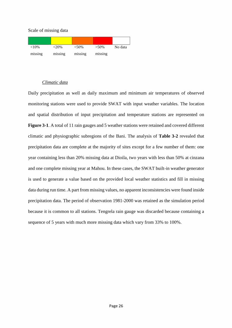
Page 26
Scale of missing data
<10%
missing
<20%
missing
<50%
missing
>50%
missing
No data
Climatic data
Daily precipitation as well as daily maximum and minimum air temperatures of observed
monitoring stations were used to provide SWAT with input weather variables. The location
and spatial distribution of input precipitation and temperature stations are represented on
Figure 3-1. A total of 11 rain gauges and 5 weather stations were retained and covered different
climatic and physiographic subregions of the Bani. The analysis of Table 3-2 revealed that
precipitation data are complete at the majority of sites except for a few number of them: one
year containing less than 20% missing data at Dioila, two years with less than 50% at cinzana
and one complete missing year at Mahou. In these cases, the SWAT built-in weather generator
is used to generate a value based on the provided local weather statistics and fill in missing
data during run time. A part from missing values, no apparent inconsistencies were found inside
precipitation data. The period of observation 1981-2000 was retained as the simulation period
because it is common to all stations. Tengrela rain gauge was discarded because containing a
sequence of 5 years with much more missing data which vary from 33% to 100%.

Page 27
Figure 3-2. Examples of quality control test failures (a) Inconsistency in daily temperature data at
Segou (b) implausible minimum temperature values at Bougouni.
Concerning temperature data, it has been noted that the original dataset contains less than 10%
missing values but are scattered with errors. Therefore, a day by day meticulous analysis was
conducted and many cases where temperature time series failed consistency and plausibility
tests have been recorded at certain locations and dates. In such cases, the erroneous data is
simply deleted and considered as missing. This technique, even though disputable, remains the
0.0
5.0
10.0
15.0
20.0
25.0
30.0
35.0
40.0
45.0
50.0
01
/01
/90
02
/01
/90
03
/01
/90
04
/01
/90
05
/01
/90
06
/01
/90
07
/01
/90
08
/01
/90
09
/01
/90
10
/01
/90
11
/01
/90
12
/01
/90
01
/01
/91
02
/01
/91
03
/01
/91
04
/01
/91
05
/01
/91
06
/01
/91
07
/01
/91
08
/01
/91
09
/01
/91
10
/01
/91
11
/01
/91
12
/01
/91
Dai
ly t
emp
erat
ure
(C
elci
us)
Date
Tmax Tmin
0.00
5.00
10.00
15.00
20.00
25.00
30.00
35.00
40.00
45.00
01
/01
/95
02
/01
/95
03
/01
/95
04
/01
/95
05
/01
/95
06
/01
/95
07
/01
/95
08
/01
/95
09
/01
/95
10
/01
/95
11
/01
/95
12
/01
/95
01
/01
/96
02
/01
/96
03
/01
/96
04
/01
/96
05
/01
/96
06
/01
/96
07
/01
/96
08
/01
/96
09
/01
/96
10
/01
/96
11
/01
/96
12
/01
/96
Dai
ly t
emp
erat
ure
(C
elci
us)
Date
Tmax Tmin
(a)
(b)

Page 28
only resort in case of datasets without appropriate metadata. Above (Figure 3-2) are some
quality control results on temperature data. Figure 3-2 (a) shows an example of inconsistency
at the Segou weather station where maximum temperature is equal to minimum temperature of
the same day and this, during the whole month of October 1991, while on Figure 3-2 (b) it can
be detected a sequence of implausible zero values in minimum temperature of December 1995
at Bougouni.
Discharge data
Daily discharge data were available at 7 monitoring stations throughout the Bani (Figure 3-1).
The analysis of the discharge record was mainly based on completeness test and visual analysis
of hydrographs and revealed the presence of high missing data. As a consequence, 1983-1997
was kept for calibration and validation processes as it is the period which exhibits few gaps at
the majority of subbasins except for Kouoro1 and Debete where 1983-1991 and 1983-1989
were available, respectively. Small existing gaps were thus filled by a simple linear
interpolation. A summary description of the available discharge monitoring stations on the Bani
for the present study is given in Table 3-3.
Table 3-3. Available discharge measurements on the Bani.
Stat_name River Country Long Lat Elev (m) Basin_area
(km2) Available data
Douna Bani Mali - 5.90 13.21 267 101000 1981-1997
Dioila Baoule Mali - 6.80 12.52 269 31573 1981-1997
Bougouni Baoule Mali - 7.45 11.40 309 14926 1981-1997
Madina Diassa Baoule Mali - 7.67 10.80 327 8417 1981-1997
Kouoro 1 Banifing Mali - 5.68 12.02 278 14487 1983-1991
Pankourou Bagoue Mali - 6.55 11.45 282 32048 1981-1997
Debete Kankelaba Cote
d'Ivoire - 6.63 10.65 336 5675 1981-1989

Page 29
3.2.4. GIS-data and databases
Soil and land use data
The soil map of the Bani was derived from the Food and Agriculture Organization of the United
Nations (FAO) Digital Soil Map of the World (DSMW) Version 3.6, completed on January
2003. The map is based on the original FAO-UNESCO Soil Map of the World published
between 1974 and 1978 and available at 1:5.000.000 scale.
We utilized the GLCC United States Geological Survey’s (USGS) a 1-km resolution Global
Land Cover Characteristics (GLCC) map version 2.0 (Loveland et al., 2000) to build the Bani
land use map. GLCC has been built with data of a 12-month period 1992-93 and therefore
represents the land cover pattern of that period.
Major soils that occur in the study catchment are mainly constituted by Luvisols, Acrisols and
Nitosols and cover a cumulative proportion of more than 97% of the total catchment area
(Figure 2-3). In addition, minor inclusions of Gleysols. Lithosols, Regosols and Cambisols can
be found. In the following, the description of the soils is summarized based on the FAO-
UNESCO legend (FAO-UNESCO, 1977) and Bouwman (1990) who provided additional
discussions on that legend.
About half of the Bani area, from the centre to the north, is covered by Luvisols and correspond
to the domains of savannah and agricultural land. Ferric luvisols are mainly formed in the
tropical zone with a long dry season and are essentially good for major food crops production
and extensive livestock raising. They possess a clay horizon, moderate organic matter content
and inherent fertility. Acrisols occur in general in warm temperate moist forest, subtropical
moist forest and subtropical moist forest. They are characterized by coarse or medium texture,
Page 30
strong acidity, very low availability of nutrients and an argillic horizon. This soil type is present
in the highlands situated in the South of the Bani where forest constitutes the principal land use
category. The principal feature of Nitosols is the high clay content which increases with depth.
In addition they are characterized by high available water capacity, variable nutrients
availability and high organic matter. With regards to Nitosols, they mostly occur in the centre
of the study catchment under savannah and in the forested zone in a lesser extent. Lithosols
and Regosols appear as inclusions in the Luvisols, while Cambisols are associated with
Nitosols and Acrisols.
Databases editing
Two databases were modified to contain custom soil and land use data and their characteristics
for the Bani: the user soils database and the crop database. Six soils namely Lithosol, Acrisol,
Cambisol, Gleysol, Ferric Luvisol and Nitosol were entered into the user soils database. We
considered 4 additional land use categories to the crop database: Forest, Savannah-Bush,
Savannah and Steppe. All the aforementioned soils and land use types as well as their
parametrization originate from the study by Laurent and Ruelland (2010).
A user weather generator database was created to store local weather stations including their
statistics. These statistics are needed by the SWAT weather generator to fill in missing values
during the running time. For this purpose, we used the excel macro WGNmaker4 (Boisramé,
2010) on the available 5 weather stations located on and around the Bani (Figure 3-1) to
calculate statistics that are representative of the local climate conditions (Neitsch et al. 2011
for details on the required weather stations statistics).

Page 31
3.2.5. Pre-processing of the SWAT input data for the Bani catchment
Four main data files are required by SWAT: Digital Elevation Model data, land use data, soil
data and weather data whereas the river network data is optional. The objective of the pre-
processing of these data files is to prepare the data specifically for the study catchment in order
to be used in the model.
GIS-data pre-processing
First, it is important to install ArcGIS and ArcSWAT, the graphical user interface for the
SWAT model. Then, spatial data were downloaded at addresses given in Table 3-1 and loaded
on ArcGIS. Following are the main steps for spatial data pre-processing:
Create a Clipping box which is a square region around the Bani;
Clip all layers by the extent of the clipping box to reduce their size;
Project the clipped layers to Universal Transverse Mercator (UTM) coordinates
because SWAT requires all input files in meter units. The Bani basin spans over
2 UTM zones: UTM Zone 29N and UTM Zone 30N. The catchment is
extending only 1.58 degree into zone 30N so we projected it into Zone 29N.
Re-clip the projected layers using the clipping box file so that any missing values that
can appear at the borders due to projection deformation are eliminated.
ArcSWAT tables and text files
There are additional necessary formatting work to be done on land use, soil and weather data
before incorporating them into SWAT.

Page 32
The land use look up table is used to make a correspondence between SWAT land cover/plant
code or SWAT urban land type code and each category in the land use map grid and was
formatted as a dBase table. Therefore, the original GLCC land use types were reclassified into
3 SWAT land use classes (Figure 3-3 and Table 3-4).
Figure 3-3. Land use/land cover maps of the Bani (a) original GLCC land cover and (b) SWAT land
use classes after reclassification.
Table 3-4. Description of the SWAT land use classes of the Bani catchment.
SWAT_LU code Description % basin area
FORE Forest 11.35
SAVA Savannah 40.3
AGRL Agricultural Land-Generic 48.35
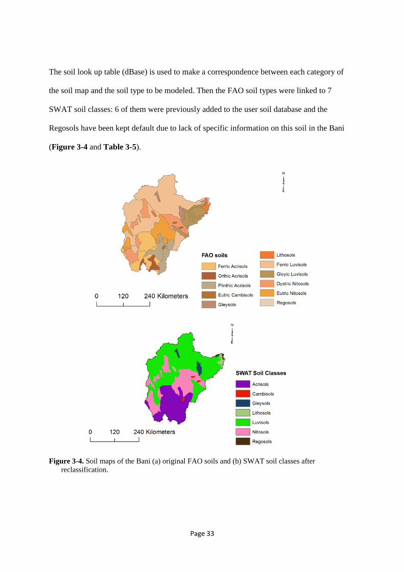
Page 33
The soil look up table (dBase) is used to make a correspondence between each category of
the soil map and the soil type to be modeled. Then the FAO soil types were linked to 7
SWAT soil classes: 6 of them were previously added to the user soil database and the
Regosols have been kept default due to lack of specific information on this soil in the Bani
(Figure 3-4 and Table 3-5).
Figure 3-4. Soil maps of the Bani (a) original FAO soils and (b) SWAT soil classes after
reclassification.

Page 34
Table 3-5. Description of SWAT soil classes of the Bani catchment.
SWAT soil class Description % basin area
Li Lithosol 1.03
Ac Acrisol 22.89
Ca Cambisol 0.18
Gl Gleysol 1.21
Lu Fe Ferric Luvisol 53.02
Ni Nitosol 21.29
*Re33-1a-1676 Regosol 0.38
*Default FAO soil type
Another type of input files required by SWAT are the gage location tables and the data tables,
both are formatted as text files. A gauge location table indicates to the model the location of
rain and temperature gauges. Therefore one precipitation gage location table was created
containing 11 gauges and one temperature gage location table with 5 weather stations. In
addition, we edited one precipitation data file containing daily precipitation for every rain
gauge and one temperature data file containing daily maximum and minimum temperatures for
every weather station to provide the model with climatic information.
Table 3-6. Precipitation gauge location table.
ID Stat_name Lat Long Elevation (m)
1 *Bamako 12.53 -7.95 369
2 *Bougouni 11.41 -7.5 343
5 *Odienne 9.5 -7.56 421
6 *Segou 13.4 -6.15 276
7 *Sikasso 11.35 -5.68 368
3 Boundiali 9.52 -6.47 415
4 Koutiala 12.38 -5.46 359
8 Kolondieba 11.1 -6.9 328
9 Dioila 12.48 -6.8 319
10 Cinzana 13.25 -5.97 281
11 Mahou 12.13 -4.63 347
*: Are temperature gauges as well.

Page 35
3.2.6. Model setup
The catchment was delineated and divided into sub-catchments based on the DEM. A stream
network was superimposed on the DEM in order to accurately delineate the location of the
streams. The threshold drainage area was kept default and additional outlets were considered
at the location of stream gauging stations to enable comparison of measured discharge with
SWAT results. The whole catchment was so discretized into 28 sub-catchments, which were
further subdivided into 181 HRUs based on soil, land use, and slope combinations. Further
parameters have been edited through the general watershed parameters and SWAT simulation
menus and are reported in Table 3-1. Four simulations were performed based on land use and
soil databases combinations: crop1soil1, crop1soil2, crop2soil1 and crop2soil2. A Nash-
Sutcliffe Efficiency (NSE) (Nash and Sutcliffe, 1970) is thereafter calculated at Douna by
comparing measured discharges against each default simulation and the one which will yield
the highest NSE value will be kept for calibration and validation processes.
Table 3-7. Input methods for SWAT model simulation on the Bani catchment.
Code Description Method
General watershed parameters
IPET Potential Evapotranspiration method Hargreaves
IEVENT Rainfall/runoff/routing option Daily Rainfall/CN runoff/Daily routing
ICN Daily Curve Number calculation
method
Soil moisture (Plant ET at Bougouni)
IRTE Channel water routing method Variable storage
SWAT simulation
Period of simulation - 1981-2000
NYSKIP Warm-up period 2 years (1981 and 1982)

Page 36
3.2.7. Calibration and validation procedures
It is commonly accepted in hydrology to split the measured data either temporally or spatially
for calibration and validation (Arnold et al., 2012a). In addition to the split-sample method, a
split-location calibration and validation approach has been performed because the global
parameters set is not expected to be optimal for sub-catchments processes in view of the high
heterogeneity in terms of climate, topography, soil and land use characterizing such a large-
area watershed. This approach is especially needed when prediction at data sparse sites is
foreseen (Moussa et al., 2007; Robson and Dourdet, 2015). In the split-sample approach, the
model was calibrated using discharge data solely measured at the catchment outlet by splitting
the homogenous period mentioned in section 2.3 into two datasets: two-third for calibration
(1983-1992), and the other one for validation (1993-1997). To implement the split-location
method, the model was calibrated at Douna and then validated at intermediate gauging stations
(Bougouni and Pankourou) by turning the model on the same period (1983-1992), using the
same behavioral parameters sets determined at the outlet.
Calibration was thereafter performed at Bougouni and Pankourou stations individually, and
both modeling frameworks facilitated a comparative analysis of model performance and
predictive uncertainty through scales. At this step, the calibration at Bougouni did not succeed
within realistic range of the Curve Number (CN). Then, the daily CN calculation method was
changed to Plant ET for simulation at Bougouni because soil moisture method is found to
predict too much runoff in shallow soils (Arnold et al., 2012a). An additional parameter
(CNCOEF) was then necessary as required by the plant ET method and fixed to 0.5 in the Edit
SWAT input menu.
Calibration/validation, uncertainty analysis and sensitivity analysis were performed within the
SWAT Calibration and Uncertainty Programs SWAT-CUP version 2012 (Abbaspour, 2014)

Page 37
using Generalized Likelihood Uncertainty Estimation (GLUE) procedure (Beven and Binley,
1992). GLUE is a Monte Carlo based method for model calibration and uncertainty analysis.
It was constructed to partly account for non-uniqueness of model parameters. GLUE requires
a large number of model runs with different combinations of parameter values chosen randomly
and independently from the prior distribution in the parameter space. The prior distributions of
the selected parameters are assumed to follow a uniform distribution over their respective range
since the real distribution of the parameter is unknown. By comparing predicted and observed
responses, each set of parameter values is assigned a likelihood value. The likelihood functions
selected here is principally the NSE as it is very commonly used and included in SWAT-CUP
for GLUE performance assessment. In this study, the number of model runs was set to 10 000
and the total sample of simulations were split into “behavioral” and “non-behavioral” based on
a threshold value of 0.5, a minimum threshold for NSE recommended by (2007) for streamflow
simulation to be judged as satisfactory on a monthly time step. In that case, only simulations
which yielded a NSE ≥ 0.5 are considered behavioral and kept for further analysis.
In the calibration procedure, we included 12 parameters that govern the surface runoff and
baseflow processes. The real approached baseflow alpha factor (ALPHA_BF) has been
determined by applying the baseflow filter program developed by (1995) and modified by
(1999) to streamflow data measured at the three outlets. One novelty in this study was to
involve the Manning's roughness coefficient for overland flow (OV_N) and the average slope
length (SLSUBBSN) parameters that are not commonly used in calibration. The reason behind
this choice was to correct the tendency of the model to delay the runoff as detected by graphical
analysis. The remaining parameters were chosen based on the literature (Betrie et al., 2011;
Van Griensven et al., 2006; Zhang et al., 2008) and their adjusting ranges from the SWAT
input/Output version 2012 document (Arnold et al., 2012b).

Page 38
3.2.8. Model performance and uncertainty evaluation
To evaluate model performance, both statistical and graphical techniques were used as
recommended by (Moriasi et al., 2007) based on previous published studies. The following
quantitative statistics were chosen: NSE to quantify the relative magnitude of the residual
variance (“noise”) compared to the measured data variance, PBIAS for water balance error and
R2 to describe the degree of collinearity between simulated and measured data, and were given
for the best simulation. The NSE, R2 and PBIAS were determined using the following equations:
2
1
2
1
1 ,
nobs sim
i i
i
nobs obs
i
i
Y Y
NSE
Y Y
(2)
2
2 1
2 2
1 1
,
nobs obs sim sim
i i
i
n nobs obs sim sim
i i
i i
Y Y Y Y
R
Y Y Y Y
(3)
1
1
100
,
nsim obs
i i
i
nobs
i
i
Y Y
PBIAS
Y
(4)
Where sim
iY and obs
iY are the ith simulated and observed discharge, respectively, sim
iY and obs
iY
the mean value of simulated and observed discharge, respectively and n the total number of
observations.
The NSE varies between - ∞ and 1 (1 inclusive), with NSE = 1 being the optimal value. The
optimal value of PBIAS is 0, with low PBIAIS in absolute values indicating accurate model
simulation. Positive values indicate model overestimation bias, and negative values indicate
model underestimation bias. R2 ranges from 0 to 1, with higher values indicating less error
variance, values greater than 0.5 are considered acceptable.

Page 39
In the present study, model performance, for a monthly time step, will be judged as satisfactory
if NSE > 0.50 and PBIAS ±25% for discharge (Moriasi et al., 2007) and if the graphical analysis
reveals a good agreement between predicted and measured hydrographs.
The GLUE predictive uncertainties were then quantified by two indices referred to as P-factor
and R-factor (Abbaspour et al., 2004). The P-factor represents the percentage of observed data
bracketed by the 95% predictive uncertainty (95PPU) band of the model calculated at the 2.5%
and 97.5% levels of the cumulative distribution of an output variable obtained through Latin
hypercube sampling. The R-factor is the ratio of the average width of the 95PPU band and the
standard deviation of the measured variable. For uncertainty assessment, a value of P-factor >
0.5 (i.e., more than half of the observed data should be enclosed within the 95PPU band) and
R-factor < 1 (i.e., the average width of the 95PPU band should be less than the standard
deviation of the measured data) should be adequate for this study especially considering limited
data availability.
3.2.9. Sensitivity analysis
A Global Sensitivity Analysis (GSA) was performed after 10,000 simulations on the 12
parameters included in the calibration process. Only GSA is allowed with GLUE in SWAT-
CUP and can be performed after an iteration. A t-test is then used to identify the relative
significance of each parameter. T-stat provides a measure of sensitivity and p-value determines
the significance of the sensitivity. A larger t-stat in absolute value is more sensitive and a p-
value close to zero has more significance (Abbaspour, 2014).
3.2.10. Verification of model outputs
To evaluate the accuracy of the SWAT model to predict PET, we considered the model average
annual basin output which was computed by the Hargreaves method (Hargreaves et al., 1985)

Page 40
and compared it to PET values calculated with two other methods: the FAO-Penman Monteith
method and the pan evaporation method. The estimates from those three methods are
hereinafter referred to as PEThar (for average annual PET estimated by the Hargreaves method),
PETpen (for average annual PET estimated by the Penman-Monteith method) and PETpan (for
average annual PET estimated by the pan evaporation method). The modified Penman method
is taken herein as the standard because it was considered to offer the best results with minimum
possible error (Allen et al., 1998). Average observed ten-day PETpen were collected and
computed to obtain average annual value on the calibration-validation period. Monthly
observed pan evaporation data were used to estimate PETpan. Doorenbos and Pruitt (1975)
related pan evaporation to reference evapotranspiration, ET0 (or PET) using empirically
derived coefficients. PET can be obtained by:
PET = × pan panK E
(5)
Where Epan represents the pan evaporation in mm d-1, and Kpan the adjustment factor that
depends on mean relative humidity, wind speed and ground cover.
As the pan factor in the Bani catchment could not be exactly determined due to lack of
information about the pan environment and the climate, the average value of 0.7 was used in
this study. The PBAIS was again used as the evaluation criterion representing the deviation of
the predicted PET compared to the one considered as the baseline.
3.3. Catchments classification
The objective of catchment classification in this study joins the second objective of
classification proposed by Sawicz et al. (2011), i.e., the regionalization of information. Indeed,
a prediction in ungauged catchments is foreseen within a data sparse region where discharge
data, if not measured, are incomplete or inconsistent. As discussed by (Hrachowitz et al., 2013;
Sawicz et al., 2014; Wagener, 2007), a holistic classification framework should combine

Page 41
physical characteristics, climate and hydrological functioning of a catchment. The major
difficulty, which lies within this classification, is the data needs. Such data are not always
available in developing regions. In addition, as the final objective is to transfer hydrological
information from gauged to ungauged catchments which are similar, the question is how to
define this similarity between them? It is evident that we need similarity metrics common for
both, easily measurable and accessible. However, no discharge data are available at the
ungauged site; neither are other runoff processes information even in well gauged catchments.
Consequently, only precipitation and physiographic parameters remain easily available
everywhere, particularly for the ungauged sites, and these are the conditions that underpin the
choice of physiographic similarity to be used in this study as a proxy of hydrological
functioning of a catchment.
3.3.1. Catchments and catchments’ attributes
A total of 28 nested candidate catchments were selected (Figure 3-5), ranging in size from 92
km2 to 10,910 km2 and spanning across a wide range of environmental gradients of topography,
precipitation, soil and land use showing a heterogeneous dataset. The study area has not been
affected by important hydraulic structures able to significantly modify their flow regimes.
The choice of catchment attributes (CAs) is of great importance. Selected CAs are related to
the shape (e.g., area, length) and the topography (e.g., slope, elevation) of each subbasin and
its main tributary reach (e.g., len1, wid1) and were derived by application of the SWAT model
(see Table 3-1 for input spatial and climatic data). The selection of the appropriate CAs can
also depend on the physical meaning of the model parameters (Mps) that will subsequently be
involved in information regionalization. For instance, in the SWAT model, the Curve Number
parameter (CN2), which was demonstrated to be the most sensitive Mps in the study area (at

Page 42
the end of the modelling process), depends on the soil and land use characteristics of the
catchment (Sellami, 2014). Therefore, two additional attributes related to land use and soil were
considered. There exist 3 land use categories (Agricultural Land Generic, Savannah and Forest)
and 3 major soil types (Ferric Luvisol, Acrisol and Nitosol, in this order).
Figure 3-5. Study catchments and Digital Elevation Model of the Bani basin.
Therefore, in the preliminary analyses, we tested 10 different land use and soil combinations:
9 combinations in which we considered 1 land use and 1 soil descriptors, and 1 combination
where all land uses and soils were kept at a time. These combinations were input in a Principal
Component Analysis and we selected the one which yielded the smaller number of dimensions
that explains the highest variability of the dataset (see the section 4.2.2 for details on the

Page 43
method). So, only Agricultural Land Generic (AGRL) and Ferric Luvisol (Lf) were retained
herein and represent indeed the dominant land use and soil, respectively. AGRL and Lf were
calculated using the following equations:
AGRL = (AAGRL
A) ∗ 100 (6)
Lf = (ALf
A) ∗ 100 (7)
Where AAGRL is the area covered by AGRL within a watershed, ALf is the area covered by Lf,
and A is the total area of the watershed.
Last, climatic characteristics such as long-term annual precipitation or the aridity index have a
relevant impact on hydrological behaviour of a catchment (Wagener, 2007), and were
commonly used in the literature. Thus, average annual precipitation was computed for each
sub-catchment on the period 1981-2000. Finally, the selection ended up with 16 physiographic
and climatic descriptors given in Table 3-8.
Table 3-8. Summary of catchment attributes derived by the SWAT model as input for multivariate
statistical analysis on the Bani catchment.
Attribute Description Units
Slo1 Subbasin slope %
Len1 Longest path within the subbasin m
Sll Field slope length m
Csl Subbasin tributary reach slope m
Wid1 Subbasin tributary reach width m
Dep1 Subbasin tributary reach depth m
Lat Latitude of the subbasin centroid dd
Long Longitude of the subbasin centroid dd
Elev Mean elevation of the subbasin m
ElevMin Minimum elevation of the subbasin m

Page 44
ElevMax Maximum elevation of the subbasin m
Shape_Leng Subbasin perimeter m
Shape_Area Subbasin area m2
*P Average annual precipitation on the subbasin mm
AGRL Proportion of Agricultural Land on the subbasin %
Lf Proportion of ferric Luvisol on the subbasin %
dd: decimal degree
* Calculated on the period 1981-2000
3.3.2. Multivariate statistical analyses
The proposed methodology can be separated into two main components: the clustering and the
analysis of dominant controls of similarity thanks to the description of explanatory variables.
Hierarchical Clustering on Principal Components
PCA and CA are frequently used in hydrological studies (Daigle et al., 2011; Kileshye Onema
et al., 2012; Sawicz et al., 2011), and commonly applied in a pre-processing of a set of variables
prior to the classification, to provide a convenient lower-dimensional summary of the dataset,
or as a classification tool itself. PCA reduces a dataset containing a large number of variables
to a dataset containing fewer new variables that are linear combinations of the original ones.
These linear combinations are mutually uncorrelated and chosen to represent the maximum
possible fraction of the variability contained in the original data and are called Principal
Components (PCs). PCs are defined each by eigenvectors, i.e., axes aligned along the direction
of the maximum joint variability of the dataset, and an eigenvalues, i.e., the variance of the PCs
(Wilks, 2006). CA is an exploratory data analysis tool that attempts to separate observations
into groups called clusters by using the degree of similarity between individual observations.
The CA procedure implemented in this study is the hierarchical and agglomerative clustering.
In the beginning of this procedure, each observation is considered as a group. In the subsequent

Page 45
steps, two groups that are closest are successively merged until, at the final step, a single cluster
is reached containing all the observations.
Multivariate statistics used in this study were performed under R package FactoMineR (Husson
et al., 2009; Lê et al., 2008), version 1.28. The methodology utilized was based on the
Hierarchical Clustering on Principal Components (HCPC) function proposed by (Husson et al.,
2010). This method combines three exploratory data analysis methods, Principal Component
methods, Hierarchical Clustering and Partitioning, to improve data analysis. The chosen
Principal Components method was the PCA, because retained CAs are quantitative variables.
PCA was used herein as a pre-process for clustering, i.e., the hierarchical clustering is solely
built on the determined PCs. In that case, a reduced dataset which represents the most important
variability in the observations was obtained, and leads to a more stable clustering than the one
obtained from original variables (Husson et al., 2010). PCA was tested on 10 datasets each
made up by the first 14 descriptors described in Table 3-1 added to a combinations of land use
(numbered 1, 2 and 3) and soils (numbered a, b and c). Therefore, the resulting input datasets
were hereinafter referred to as 1-a, 1-b, 1-c, 2-a, 2-b, 2-c, 3-a, 3-b, 3-c, and 123-abc, the latter
referring to the dataset including all land uses and soil types. Input variables, i.e., CAs, were
first standardized because they are not measured on comparable scales. The appropriate number
of PCs was chosen based on the Scree plot technique (Jolliffe, 2002). The Scree plot is a graph
representing the eigenvalues as a function of PCs number. On this graph, the point separating
a steeply sloping portion and a gently one, corresponds to the truncated number of PCs. As the
objective of PCA used in this study was for dimensionality reduction, then the combination
that will give no more than 2 PCs that explain the highest percentage of the total variance of
the original data, will be kept for subsequent analysis. Then, a hierarchical agglomerative
clustering was performed on the PCs previously determined. The measure of distance between
data points was based on the Euclidean distance (the same was used in PCA) and the

Page 46
agglomerative method for merging two clusters used the Ward's criterion. This criterion is
based on the Huygens theorem according to which the total inertia (variance) of a dataset can
be decomposed in within-group and between-group inertia. Equation (3) gives the formula for
calculating the total inertia.
2
2 2
1 1 1 1 1 1 1 1
,q qI IQ Q QK K K
qkiqk k q k iqk qk
k q i k q k q i
x x I x x x x
(8)
Total inertia = Between-group inertia + Within-group inertia
Where xiqk is the value of the variable k for the individual i of the cluster q, qkx is the mean of
the variable k for cluster q, kx is the overall mean of variable k and Iq is the number of
individuals in cluster q. At the initial stage, the within-group inertia is null and the between
group inertia is maximum and equal to the total inertia of the dataset as at this level, each
individual represents a single-member group. At the final step, all the members are merged in
a single group, the between-group inertia is therefore null and the within-group inertia is
maximum and equal to the total. At each step of the algorithm, the pair of groups to be merged
is chosen that minimizes the growth of within-group inertia (inversely, that maximizes the
growth of between-group inertia) at each step of the algorithm.
The last step consists in choosing the appropriate number of clusters when it is not pre-assigned,
that is, the stopping point of clustering that maximizes similarity within clusters and maximizes
dissimilarity between clusters. HCPC function suggests an “optimal” number Q of clusters
when the decrease in within-group inertia between Q - 1 and Q is from far greater than the one
between Q and Q + 1 (Husson et al., 2010) for a thorough description of the HCPC function).
Results of HCPC function can be presented in different ways: (1) A factor map, which displays
results of the hierarchical clustering on the map induced by the first PCs, (2) a 2-dimensional
dendrogram or hierarchical tree, and (3) a 3-dimensional dendrogram in which the hierarchical

Page 47
tree is incorporated into the factor map. The latter representation can solely be used to get an
integrated visualization of the dataset. However, dispersion of data points is somehow masked
in that way. Therefore, the factor map was presented in the results section for a better
visualization of individuals’ dispersion on the plan formed by PCs, while the hierarchical tree
offers a good insight of the variability increase between clusters.
Analysis of dominant causes of similarity between catchments
A core issue in catchment classification is to describe clusters according to the main factors
that cause similarity among individuals. Addressing this issue will help knowing, in addition
to which catchments are similar, why they are similar. This can be achieved through the
description of input variables, i.e., CAs. A v-test was performed for each variable
corresponding to the test: “The mean of the category is equal to the overall mean”. The mean
of the category is the average in the cluster and the overall mean is the average for the whole
data set. An absolute value of the v-test greater than 1.96 means that the variable is significant.
The sign of the v-test indicates whereas the mean of the cluster is lower or greater than the
overall mean. A p-value less than 0.05 gives the significance of the test (more details can be
found in (Husson et al., 2011).
The v-test is calculated with the following Equation (4):
2
1
qk kx xv test
S N n
n N
(9)
where qkx is the mean of the variable k for cluster q, kx is the overall mean of variable k, n is
the number of individuals in cluster q, N is the total number of individuals and S² is the variance
of the dataset.

Page 48
3.4. Model Parameters Regionalization
3.4.1. Study catchments and modeling framework
This study was conducted on the Bani catchment for which a detailed description was given in
sections 3.2 and 3.3. A total of seven mesoscale catchments, ranging in size from 1,552 to
8,417 km2, were selected (Figure 3-6) on the basis of data availability and span across different
physiographic and climatic regions (catchments description is given in Table 3-9). It is
important to note that the study area is characterized by weak data density (around 7 stream
gauges per 100,000 km2) and high distances between gauges (more than 300 km for the
highest).
Calibration at gauged catchment is a prerequisite for regionalization of model parameters. To
this end, we calibrated the SWAT model against a 10-year discharge record (1983-1992) and
validate it on 5 other years (1993-1997) for most of the catchments. The adjustment between
observed and simulated river flow has been achieved by tuning 12 SWAT model parameters
identified as the most sensitive on the study area. The approach of estimating these parameters
has been developed in section 3.2.7 for calibration and validation at Douna, Pankourou and
Bougouni gauging stations. The same approach was adopted here for the 4 additional stations;
Dioila, Kouro 1, Madina Diassa and Debete (Figure 3-6 and Table 3-9). We defined a
behavioral parameter set, as the one which produced a simulation with a NSE equal to 0.5 or
greater. When the calibration task identifies one or more behavioral parameter sets on a
catchment, this one is considered as a donor catchment, i.e., from which the optimized model
parameters could be transferred to an ungauged catchment, else it is solely considered as a
target catchment, i.e., it can only receive model parameters from a potential donor.

Page 49
Figure 3-6. Localization of the test catchments for model parameters transfer on the Bani basin.
Table 3-9. Description of candidate catchments for model parameters regionalization.
Subbasin Outlet Area
(km2)
*Physical
cluster
Precipitation
(mm)
Calibration
period
Regionalization
period
1 Douna 5925 C2 653 1983-1992 1983-1997
4 Dioila 3333 C2 794 1983-1992 1983-1997
7 Kouoro1 1552 C1 842 1983-1991 1983-1991
16 Pankourou 1620 C3 1036 1983-1992 1983-1997
18 Bougouni 2978 C3 1107 1983-1992 1983-1997
25 Debete 5675 C4 1294 1983-1989 1983-1989
26 Madina Diassa 8417 C4 1200 1983-1992 1983-1997
*See Chapter IV for details.

Page 50
3.4.2. Regionalization approaches and similarity frameworks
In this study, the objective of the regionalization is to predict the entire discharge hydrograph,
i.e., the time series of river discharge, at ungauged basins. The hydrograph has the advantage
to be “… the most complete runoff signature…” Blöschl et al. (2013) because resulting from
the interaction between all the processes within a catchment. So, all the other signatures can be
derived from it. We applied 2 regionalization techniques based on similarity measure between
gauged and ungauged catchments. The first approach is the spatial proximity, according to
which catchments that are geographically close to each other are expected to have similar
behavior. The nearest neighbor method is especially relevant in the case of very data sparse
region (Goswami et al., 2007). In this study, the entire model parameter set is transposed from
the closest donor to the receptor catchment. The distance measure between catchments is
defined by the geographical distance between catchments’ centroids. In the physical similarity
approach, the search of donor catchment was restricted to the same cluster as the target
catchment. As an important step in physiographic similarity, a classification scheme was
conducted prior to the regionalization (in Chapter III) to determine clusters of similar
catchments based on their physioclimatic characteristics. A combined method can be
interpreted as when the donor is physically similar to the ungauged catchment and is located in
its vicinity as well.
However it has been pointed out that the MPs from the nearest catchment will not necessarily
result in the best simulation at the target catchment (Oudin et al., 2008). In addition, many
authors (Patil and Stieglitz, 2012; Viviroli et al., 2009) suggest the use of multiple neighbors
in order to find the best regionalization efficiency. But such an approach is not possible in the
present study because we are in a case of very data-sparse region. The stream gauge density
considered is low, (1 gauge per 14300 km2) and a gauge catchment can be very far from an
ungauged catchment. Therefore, to avoid misleading effects of small number of test

Page 51
catchments, we considered all the possible cases on model parameters transfers without any
consideration of spatial or physical similarity. In other words, if n is the total number of donors,
at a target i, we transferred one by one, the parameter set of the n-1 donors, resulting in n-1
individual simulations. The entire set of optimized SWAT model parameters is transposed
without any modification from the donors to the target catchment to achieve discharge
hydrograph without need of any measurement. The resulting simulations were then discussed
according to the aforementioned regionalization methods to draw conclusions and hypotheses
related to which method performs best.
3.4.3. Evaluation of the regionalization performance and prediction uncertainty
The aim of this step is to assess the performance and prediction uncertainty of parameters
regionalization in reproducing flows in ungauged basins. For this assessment, the Nash-
Sutcliffe Efficiency (NSE) was calculated between the simulated and observed hydrographs for
the entire simulation period 1983-1997. The length of the regionalization period has been
chosen long enough to cover both calibration and validation periods at gauged catchments. So,
we can test at a time the reliability of the transfer of MPs to perform under different flow
conditions of space (from gauged to ungauged) and time (from calibration to validation period).
The performance was judged as satisfactory if NSE > 0.50 and PBIAIS < ±25%, and if the
graphical analysis reveals a good agreement between predicted and measured hydrographs.
Regarding uncertainty assessment, the P-factor was used to measure the percentage of observed
data enclosed within the uncertainty band whose width is represented by the R-factor. In this
study, we define adequate prediction uncertainty when we obtained a value of P-factor > 0.5
(i.e., more than half of the observed data are enclosed within the 95PPU band) and R-factor <
1 (i.e. the average width of the 95PPU band is less than the standard deviation of the measured
data) especially considering limited data availability.

Page 52
3.4.4. Assessment of the hydrological similarity
Many definitions of hydrological similarity exist. Following Oudin et al. (2010), hydrological
similarity between two catchments can be defined as the ability of the optimized parameter set
of one to adequately simulate the streamflow of the other. This assumption explains the use of
a rainfall-runoff model for making prediction in ungauged catchments.
Our objective is to explore the relationship between spatial proximity and physical similarity
on one hand, and hydrological similarity on the other. To this end, the performances of the
resulting hydrographs are compared in order to identify the approach that gives the highest
performance. We adopted the criterion defined by Oudin et al. (2010) who suggest that two
catchments A and B are hydrologically similar “if, on target catchment A, the efficiency
reached by the model using the parameters obtained by calibration on catchment B is greater
than 0.9 of the model efficiency obtained in calibration on catchment A, then this catchment B
is considered as hydrologically similar to catchment A”. That means, all catchments should be
calibrated so that a comparison between efficiencies obtained by calibration and by
regionalization is feasible. We adapted this definition to our context of data scarcity and say:
if the performance reached at the target using the parameters obtained at the donor is greater
than 0.5, 0.65 or 0.75 the performance reached by calibrating at the target, then the hydrological
similarity between donor and target can be judged as satisfactory, good or very good,
respectively. In addition, the transfer of parameters from one to another should work in both
ways in order to call the catchments “mutually similar”.

Page 53
Chapter IV

Page 54
4. Results and Discussions
4.1. Multi-site Validation of the SWAT Model on the Bani Catchment:
Model Performance and Predictive Uncertainty*
*Results published in Chaibou Begou et al. (2016)
Reference:
J. Chaibou Begou, S. Jomaa, S. Benabdallah, P. Bazie, A. Afouda, and M. Rode, (2016).
Multi-site validation of the SWAT model on the Bani catchment: Model performance and
predictive uncertainty. Water, 8, 178.

Page 55
The objective of this Chapter is to assess the performance of the SWAT model and its predictive
uncertainty on the Bani at catchment and subcatchment levels. More specifically, this meant
to:
(i) set up a hydrological model for the Bani catchment using the SWAT program;
(ii) calibrate the model at the catchment outlet at daily and monthly time steps and
assess the prediction performance and uncertainty;
(iii) evaluate the spatial performance of the watershed-wide model within the catchment
by validating it at two internal stations
(iv) And calibrate the model at the sub-catchments separately and provide a comparative
assessment of the model performance at different spatial scales.
4.1.1. The catchment scale model
Global model performance and predictive uncertainty
In the preliminary analyses we tested different land use and soil databases and kept for
subsequent analysis the simulation of databases combination crop2soil2, which yielded the
highest default, i.e. before calibration, performance (NSE = 0.09). The impact of land use
database was not so significant, but the type of soil database used to setup the model was very
decisive in obtaining a simulation with the smallest overall error. SWAT-CUP output results
are presented as 95PPU as well as the best simulation (Table 4-1).
Overall, calibration and validation of the hydrological model SWAT on the Bani catchment at
the Douna outlet yielded good results in terms of NSE and R2 for both daily and monthly
timesteps. 364 simulations for daily calibration against 588 for monthly calibration returned a
NSE ≥ 0.5 and were thus considered as behavioral. Satisfactory to very good NSE and R2 values
were obtained and were greater than 0.75 for the best simulations. Moreover, it can be noticed

Page 56
that the performance is slightly lower for daily calibration compared to monthly calibration,
but always higher for the validation period. Only one year (1984) over ten showed very low
performance with a NSE of 0.23.
Table 4-1. Model performance statistics and predictive uncertainty indices of the SWAT model for
the Bani catchment at Douna, Pankourou and Bougouni discharge gauging stations.
Time
step
Calibration (1983-1992) Validation (1993-1997)
Criterion Douna Pankourou Bougouni Douna Pankourou Bougouni
Daily
NSE 0.76 0.73 0.66 0.85 0.77 0.37
R2 0.79 0.74 0.68 0.87 0.83 0.57
PBIAS (%) - 12.23 6.08 - 15.01 - 23.26 - 19.57 - 59.53
P-factor 0.61 0.68 0.60 0.62 0.63 0.51
R-factor 0.59 0.41 0.57 0.51 0.29 0.35
Monthly
NSE 0.79 0.78 0.72 0.85 0.81 0.47
R2 0.82 0.78 0.76 0.88 0.91 0.68
PBIAS (%) - 15.78 5.93 - 13.14 - 26.91 - 19.54 - 58.40
P-factor 0.65 0.71 0.58 0.70 0.67 0.55
R-factor 0.65 0.45 0.54 0.55 0.31 0.32
The water balance prediction can be considered as accurate at a daily time-step but become
hardly satisfactory for monthly calibration, which is characterized by higher PBIAIS values
showing increasing errors in the prediction. For example, the PBIAIS values increased from
daily to monthly time intervals: from - 12% to - 16% in the calibration period and from - 23%
to - 27% in the validation period (Figure 4-1). With regard to high flow events, visual analysis
of simulated and observed hydrographs represented in Figure 3 came out with the following
results: timing of peak is well reproduced although simulation tends to underestimate peak
flows especially during dry years (e.g., 1983, 1984, and 1987).
The predictive uncertainty of the model, as indicated by the P-factor and R-factor, is adequate,
though being larger during peak flow and recession periods (reflected by larger 95PPU band).
On a daily basis for instance, 61% of the observed discharge data are bracketed by a narrow

Page 57
95PPU band depicted by the R-factor < 1 (Figure 4-1). It has been noted that the entire
uncertainty band is, however, very large during the year 1984.
Figure 4-1. Simulated and observed hydrographs at Douna station at (a) daily and (b) monthly
timesteps along with calculated statistics on calibration and validation periods.
Verification of average annual basin values
Table 4-2 reports the average annual values of the SWAT model simulated on the Bani
catchment. However, there are not available data to enable a full verification of all model
outputs at the watershed scale. In this case, we focused on available PET and biomass for which
there exist regional values.

Page 58
Table 4-2. Average annual basin values of precipitation (P), Evapotranspiration (ET), Potential
Evapotranspiration (PET) and biomass as SWAT outputs on the Bani catchment.
Period P (mm) ET (mm)
PET (mm)a
Biomass (ton ha-1)
Agricultural
Land Generic Savannah Forest
Calibration
(1983-
1992)
960.4 895 1925.7 1.18 0.27 3.09
Validation
(1993-
1997)
1049.5 975 1925.1 1.72 0.53 5.51
a Average annual PET estimated by the Hargreaves method (herein used by SWAT).
The analysis of Table 4-2 came out with several results. On average, PEThar presented a
positive PBIAS of 11% compared with observed PETpen herein equal to 1737 mm and the
latter is very close to PETpan estimated to 1755 mm. These results give a clear advocate of
overestimation of PET by the SWAT model over the Bani catchment, an overestimation that
can be attributed to the Hargreaves method used herein by the model to compute PET.
To further investigate the model’s accuracy, we evaluated predicted biomass values over the
calibration/validation period against reported values for the study area. Simulated biomass was
on average 4.3 ton ha-1 for forest and 1.45 ton ha-1 for agricultural land and both are in the
ranges of observed values in the region (Laurent and Ruelland, 2010; Marie et al., 2007).
Nevertheless, this component is far underestimated for savannah with a simulated value of 0.4
ton ha-1.
Sensitivity analysis
There is a wide range of uses for which sensitivity analysis is performed. Based on the 12
selected SWAT parameters (ALPHA_BF being fixed), a GSA was used herein for identifying
sensitive and important model parameters in order to better understand which hydrological
processes are dominating the streamflow generation in the Bani catchment.

Page 59
Sensitivity analysis results of 10 000 simulations are summarized in Table 4-3. The first three
most sensitive parameters (CN2, OV_N and SLSUBBSN) are directly related to surface runoff,
reflecting therefore the dominance of this process on the streamflow generation in the Bani
catchment. Processes occurring at soil level followed at the second position as pointed out by
the sensitivity of ESCO and SOL_AWC. Groundwater parameters happened in the last position
demonstrating the low contribution of the latter to flows measured at the Douna outlet. The
same sensitive parameters were identified by daily and monthly calibrations with only different
ranks for soils parameters (ESCO and SOL_AWC).
Table 4-3. Sensitivity of the calibrated SWAT model parameters on the Bani catchment at Douna on a
daily time interval.
Parameter Description Input calibration
range
Global Sensitivity
analysis
t-stat p-value
CN2 SCS runoff curve number II (-) ± 20% - 54.03083 0.00000
OV_N Manning's "n" value for overland flow (-) 0.01-30 11.41603 0.00000
SLSUBBSN Average slope length (m) 10-150 8.87352 0.00000
ESCO Soil evaporation compensation factor (-) 0.01-1 - 6.08880 0.00000
SOL_AWC Available water capacity of the soil layer
(mm H2O/mm sol) ± 20% 2.89864 0.00376
GW_DELA
Y Groundwater delay (days) 0.0-50 1.81341 0.06980
GWQMN
Threshold depth of water in the shallow
aquifer required for return flow to occur
(mm H2O)
0.0-4000 - 1.51853 0.12891
REVAPMN Threshold depth of water in the shallow
aquifer for "revap" to occur (mm H2O). 0-500 - 0.64939 0.51610
RCHRG_D
P Deep aquifer percolation fraction (-) 0-1 0.46408 0.64260
GW_REVA
P Groundwater "revap" coefficient (-) 0.02-0.2 - 0.12613 0.89963
SURLAG Surface runoff lag coefficient (-) 0.05-24 - 0.07433 0.94075
ALPHA_BF Baseflow alpha factor (d-1) 0.034-0.034 ND ND
ND: Not Determined

Page 60
Spatial validation
The results of the spatial validation were divergent according to the location (Figure 4-2). For
instance at Pankourou, the same parameters sets determined at Douna produced a good
simulation on a monthly basis (satisfactory for daily validation) whereas predictive uncertainty
remained adequate and all met our requirements (NSE > 0.5, P-factor > 0.5 and R-factor < 1).
In addition, the water balance was reasonably predicted at both timesteps. In contrast, it has
been recorded a complete loss of model performance at Bougouni with unsatisfactory NSE
values and more uncertainty related to input discharge as expressed by a lower percentage of
observed data (P-factor = 0.55 et 0.57 for daily and monthly validation) inside the 95PPU band
(Figure 4-2). Accordingly, important uncertainty could be attributed to observed discharge at
Bougouni.
Figure 4-2. Spatial validation of the SWAT model on the Bani catchment. The model was turned at
Pankourou ((a) daily and (b) monthly timesteps) and at Bougouni ((c) daily and (d) monthly

Page 61
timesteps) by using the same behavioral parameter sets determined at the Douna outlet on the
period 1983-1992.
4.1.2. The subcatchment model
Statistical evaluation results of the subcatchment calibration are presented in Table 4-1 and
time series of observed and simulated hydrographs are shown on Figures 4-3 and Figure 4-
4. Good to very good performance was obtained at Pankourou with accurate predictive
uncertainty. However the validation period remained unsatisfactorily simulated at Bougouni.
A comparative analysis of the catchment and subcatchment calibration performances came
out with the following results:
When calibrated separately, the prediction at Pankourou was slightly better, but greatly
improved at Bougouni compared to when the catchment wide model was applied.
The total uncertainty of the model is smaller at Pankourou (smaller R-factor and larger P-
factor) than at the whole catchment, but larger at Bougouni.
The water balance is better simulated at both internal stations compared to the watershed-
wide water balance as depicted by smaller PBIAIS values, except always in the validation
period at Bougouni.
The model performance in terms of NSE and R2 was higher at the watershed-wide level
than at the sub-watershed level.
Overall, these results revealed that further calibration at the internal gauging stations was
synonymous with gain of performance at the subcatchment level.

Page 62
Figure 4-3. Simulated and Observed hydrographs at Pankourou station at (a) daily and (b) monthly
timesteps along with calculated statistics on calibration and validation periods.
Figure 4-4. Predicted and measured discharges at Bougouni station at (a) daily and (b) monthly
intervals during the calibration and validation periods with their corresponding statistics.

Page 63
4.1.3. Discussion and conclusions
Model performance and predictive uncertainty
In an effort to assess the performance of the SWAT model on the Bani catchment, we calibrated
and validated the model at multiple sites on daily and monthly timesteps by using measured
climate data. There were no statistically significant differences in model performance among
time intervals. Using guidelines given in Moriasi et al. (2007), the overall performance of the
SWAT model in terms of NSE and R2 can be judged as very good especially considering limited
data conditions in the studied area. On a monthly basis, we obtained at the Douna outlet a NSE
value equal to 0.79 for the calibration period (0.85 for the validation period). These results are
greater than the ones of the studies by Schuol and Abbaspour (2006) and Schuol et al. (2008a)
at the same outlet. Schuol and Abbaspour (2006) reported indeed a negative NSE (between -1
and 0) for the monthly calibration and a value ranging between 0 and 0.7 for monthly
validation, while (Schuol et al., 2008a) obtained a NSE between 0 and 0.70 for both monthly
calibration and validation. However, Laurent and Ruelland (2010) reported a greater
performance (NSE values varying between 0.81 and 0.91 for calibration and validation period,
respectively) but on a coarser time step (average annual basis). The water balance is less well
simulated, especially for monthly time step with a PBIAIS greater than 25% in absolute value.
The quantified predictive uncertainties are surprisingly satisfactory. At the end of the daily
calibration, the model was able to account for 61% of observed discharge data (65% for
monthly calibration) in a narrow uncertainty band. The quantified predictive uncertainties
obtained herein are close to the results of (Schuol et al., 2008a) who estimated the observed
discharge data bracketed by the 95PPU between 60% and 80% for monthly calibration (40%
and 60% for monthly validation). However, one explanation that could be attributed to the
Page 64
small uncertainty band we obtained, is that model predictive uncertainty derived by GLUE
depends largely on the threshold value to separate “behavioral” from “non-behavioral”
parameter sets (Mantovan and Todini, 2006; Montanari, 2005).This means, a high threshold
value (as in this case) will generally lead to a narrower uncertainty band (Blasone et al., 2008;
Viola et al., 2009; Xiong and O’Connor, 2008) but this will be achieved at the cost of bracketing
less observed data within the 95PPU band. In addition, GLUE accounts partly for uncertainty
due to the possible non-uniqueness (or equifinality) of parameter sets during calibration and
could therefore underestimate total model uncertainty. For instance, Sellami et al. (2013)
showed that the GLUE predictive uncertainty band was larger and surrounded more
observation data when uncertainty in the discharge data was explicitly considered. Engeland
and Gottschalk (2002) demonstrated that the conceptual water balance model structural
uncertainty was larger than parameter uncertainty. In spite of all the aforementioned limitations
of GLUE, we succeeded in enclosing interestingly most of the observed data within a narrow
uncertainty band (the sought adequate balance between the two indices) hence increasing
confidence in model results. These are encouraging results showing, on one hand, the good
performance of the SWAT model on a large soudano-sahalian catchment under limited data
and varying climate conditions and, on the other hand, the capability of observed climate and
hydrological input data of this catchment, even though contested, to provide reliable
information about hydro-meteorological systems prevailing in the region.
It has been also noted that the model did not perform well during the year 1984 particularly
(lower performance and larger uncertainty). This loss of performance can be attributed to the
disruption in rainfall-runoff relationship consequence of consecutive years of drought, which
has prevailed in the beginning of the eighties. The over-predicted PET on the Bani catchment
could be attributed to the Hargreaves method, which could give a greater estimate of PET than
it actually is. Ruelland et al. (2012) applied a temperature-based method given by Oudin et al.

Page 65
(2005) and provided a similar estimate of PET (1723 mm) than the values calculated herein by
the Penman and pan evaporation methods hence corroborating our results. These results
demonstrated the valuable of pan evaporation measurements for estimating PET and that the
simple pan evaporation method appears to be suited for application in the study area and can
be used when all the climatic data required by the Penman method are missing.
As far as biomass is concerned, the underestimation of this component in savannah could be
explained by inappropriate specification of all categories in the land use map grid to be
modelled by SWAT as savannah or inaccurate savannah characteristics added in the SWAT
database and directly affecting biomass production such as BIO_E and LAI parameters, among
others.
Advance in understanding of hydrological processes
The GSA confirms what has already been reported on and around the Bani catchment about
the contribution of hydrological processes to streamflow generation. In order to better
understand the origin of flows at Kolondieba (a tributary of the Bani River), Dao et al. (2012)
showed that Groundwater contribution to the hydrodynamic equilibrium at the outlet of
watershed Kolondieba is small and the direct flow from the soil surface governs the runoff
process. This fact can be explained by the double impact of a general impoverishment of
shallow aquifers due to reduction in precipitation in West Africa in general since the great
drought of the seventies as well as a concurrent increase of the recession coefficient of the Bani
river as demonstrated by Bamba et al. (1996) and Mahé (2009) with a decrease of baseflow
contribution to total flow in absolute and relative values as corollary.
Page 66
Spatial performance
The results of different calibration and validation techniques showed varying predictive
abilities of the SWAT model through scales. Firstly, it can be derived from these findings that
model performance in terms of NSE and R2 was higher on the watershed-wide level than on the
sub-watershed level. However, this could be attributed to a compensation between positive and
negative errors of processes occurring at a larger scale (Cao et al., 2006; Wellen et al., 2015).
This suggests that calibrating a model only at the basin outlet leads to an overconfidence in its
performance than at the sub-basin scale. Secondly, individual calibration of subcatchment
processes expectedly improved model accuracy in predicting flows at the internal gauging
stations, due to reducing heterogeneities with downsizing space, and is especially beneficent
while the donor and receiver catchments are substantially different. Finally, prediction
uncertainty appears to decrease with reducing spatial scale but increases with humidity as
shown by the lower performance recorded at Bougouni. The inability of the model to perform
during the validation period at Bougouni could be attributed to the structure of the validation
period which is substantially different to that of calibration, and is solely composed by average
to wet years while in contrast, it is noted the occurrence of dry, average and wet years during
the calibration period.
These results have an important role to play in the calibration and validation approaches of
large-area watershed models and constitutes a first step to model parameters regionalization
for prediction in ungauged basins.
Conclusions
In this study, the performance of the widely-used SWAT model was evaluated on the Bani
catchment using both split-sample and split-location calibration and validation techniques on
daily and monthly intervals. The model was calibrated at the Douna outlet and at two internal

Page 67
stations. Freely available global data and daily observed climate and discharge data were used
as input for model simulation and calibration. Calibration and validation, uncertainty and
sensitivity analyses were performed with GLUE within SWAT-CUP. Both graphical and
statistical techniques were used for hydrologic calibration results evaluation.
Evapotranspiration and biomass production outputs were verified and compared to regional
values to make sure these components were reasonably predicted. Sensitivity analysis
contributed to a better understanding of the hydrological processes occurring at the study area.
Final results showed a good SWAT model performance to predict daily as well as monthly
discharge at Douna with acceptable prediction uncertainty despite the poor data density and the
high gradient of climate and land use characterizing the study catchment. This performance is
somehow lower at internal sub-catchments level when the global parameters sets are applied,
especially at the one with higher humidity and dominated by forest. However, subcatchment
calibration induced an increase of model performance at intermediate gauging stations as well
as a decrease of total uncertainty. With regard to predicted PET, this component is
overestimated by the model when the Hargreaves method is applied in that specific region
while biomass production remained low in savannah land use category. The GSA revealed the
predominance of surface and subsurface processes in the streamflow generation of the Bani
River.
Overall, this study has shown the validity of the SWAT model for representing globally
hydrological processes of a large-scale soudano-sahelian catchment in West Africa. Given the
high spatial variability of climate, soil and land use characterizing the catchment, additional
calibration is however needed at subcatchment level to ensure that predominant processes are
captured in each subcatchment. Accordingly, the importance of spatially distributed
hydrological measurements is demonstrated and constitute the backbone of any type of
progress in hydrological process understanding and modeling. The calibrated SWAT model for

Page 68
the Bani can be used to assess the current and future impacts of climate and land use change
on water resources of the catchment, a more and more necessary information awaited by water
resources managers. Knowing this information, a strategy of adaptation in response to the
current and future impacts can be clearly proposed and the vulnerability of population can
therefore be reduced. More widely, this impact study can increase the transferability of the
model parameters from the Bani subcatchment to another ungauged basin with some
similarities, and then predicting discharge without the need of any measurement. These
findings are very useful especially in West Africa, where many river basins are ungauged or
poorly gauged.

Page 69
4.2. Catchment Classification: Multivariate Statistical Analysis for
Physiographic Similarity*
*From the original idea of Chaibou Begou et al., 2015
Reference:
J. Chaibou Begou, P. Bazie and A. Afouda, (2015). Catchment classification: multivariate
statistical analyses for physiographic similarity in the Upper Niger Basin. IJERA Vol. 5, Issue
9, (Part - 1), pp.60-68

Page 70
The main objective of this chapter was to determine a physiographic and climatic similarity
framework between catchments located on the Bani basin. The specific objectives were to:
(1) Perform a hierarchical clustering of catchments based on their physiographic and climatic
characteristics
(2) And determine the main factors that control similarity between catchments.
This study provides the first ever quantification of similarity among catchments with respect
to physiographic characteristics on a large tropical river basin at finer spatial scale. Neither
descriptors, nor statistics themselves are actually novel in the broad literature, but their
combined use in that particular area to evaluate the gain of homogeneity with increasing
number of clusters is sought. In other words, the questions that will be addressed in this study
are:
(i) Can the Bani be further separated into similar groups of catchments based on
physio-climatic characteristics?
(ii) If so, what are the dominant controls on similarity between catchments?
(iii) And how much do we gain in system homogeneity when moving from the whole
dataset to the optimal number of groups?
4.2.1. Catchments clustering
In this section, a brief description of the intermediate results of PCA is given. PCA was repeated
10 times and the most successful result was recorded on the combination 1-a, that permitted to
determine 2 PCs which explains the highest cumulative variance (76.10%) as compared to
other combinations that gave either smaller variance or more PCs. Results can be visualized on

Page 71
Figure 4-5. The percentage of the joint variability of the original dataset explained by each
dimension is also given. The subsequent clustering was then performed on retained PCs.
Results of the hierarchical clustering are presented on Figures 4-5 and 4-6. Figure 4.5 displays
results of the hierarchical clustering on the map induced by the first PCs. Four clusters were
identified that maximize the within-group similarity while maximizing the between-group
dissimilarity. Cluster 1 (C1) contains 5 catchments (4 catchments if we consider the number
21 as an outlier).
Figure 4-5. Hierarchical clustering representation on the map induced by the first 2 Principal
Components on the Bani catchment. Sub-catchments are coloured according to the cluster they
belong to, the barycenter of each cluster is represented by a square and Dim1 and Dim2 are the
first two Principal Components on which the hierarchical clustering is built.
It is worth noting that these catchments have the smallest sizes in the dataset and their metrics
(especially the area) could provide a bias in the distribution. In this group C1, it is found Kouoro
1 (sub-catchment 7). The second cluster (C2) is made up of 7 subbasins, among which, Douna

Page 72
and Dioila (subbasins 1 and 4, respectively). The third Cluster (C3) represents a large mixing
of 13 similar subbasins, such as Pankourou (subbasin 16) and Bougouni (subbasin 18). Finally,
cluster 4 (C4) is considered as being well dissimilar to other clusters and is formed by the
combination of 3 catchments; the well-known are Debete (25) and Madina Diassa (26).
Beside the optimal number of clusters suggested by the HCPC algorithm, one can look for a
reorganization of clusters by examining the hierarchical tree illustrated on Figure 4.6. The tree
represents the inertia loss as a function of clustering steps. The point at each two catchments
that are merged is represented by the horizontal branch linking them, and the inertia loss
attributed to this merging is read by projecting orthogonally the horizontal branch on the
vertical axis. First, it can be noticed that C3 and C4 are closest to one another (the horizontal
branch linking them is lower than the one linking C1 and C2 and could be merged into one
cluster by increasing the variability of the system by 1.98. Then, the other merging possibility
is between C1 and C2 but at the expense of increasing the variability by 2.94. Therefore, this
classification into 2 clusters (C3+C4, C1+C2) could be envisaged depending on the application,
which the classification is intended for.
In addition, the analysis of the barplot of within-group inertia (Figure 4-6) highlights an
important outcome: The loss of inertia (variability) or inversely the gain of homogeneity in the
system with increasing number of clusters. It is worth noting that the loss of inertia when
moving from one cluster to two, is equal to 3.62, from 2 clusters to 3, 2.94, and from 3 to 4,
1.98 (can be read on the barplot). So, from a single cluster to the optimal number of 4 clusters,
we reduced the variability by 8.54 and gained, therefore, in more system homogeneity.

Page 73
Figure 4-6. Hierarchical dendrogram of the Bani catchment. Each rectangle represents a cluster of
similar catchments. The barplot (inertia gain) gives the decrease of within-group variability with
increasing number of clusters.
4.2.2. Major controlling factors of similarity
It is important to explain the causes of similarity inside each cluster by determining attributes
that are exerting strong control on each cluster. The description of input variables is given in
Table 4-4. Results are also enriched by the analysis of the spatial distribution of clusters given
in Figure 4-7.

Page 74
Table 4-4. Description of hierachical clusters. In bold, positive v-test values indicate the variable that
has a value greater than the overall mean, and in italic, negative v-test values refer to the variable
that has a value smaller than the overall mean. All v-test values are significant at the probability
p = 0.05.
Variable v-test Mean in category Overall mean p-value
Cluster 1
Shape_Area - 2.96 728.24 3623.44 0.003104
Len1 - 3.43 56277.76 135344.70 0.000601
Wid1 - 3.52 62.95 166.14 0.000428
Shape_Leng - 3.62 192137.08 465762.00 0.000296
Dep1 - 3.78 1.69 3.24 0.000160
Cluster 2
AGRL 2.97 87.75 50.81 0.002936
Lat 2.76 12.17 11.41 0.005818
Lf 2.74 91.25 56.71 0.006213
ElevMin - 2.68 265.57 285.96 0.007257
P - 3.00 829.56 1011.18 0.002674
Cluster 4
Slo1 3.95 3.53 2.12 0.000080
ElevMax 3.41 801.67 559.00 0.000654
Elev 3.25 405.79 352.47 0.001171
ElevMin 2.77 321.00 285.96 0.005648
P 2.67 1279.97 1011.18 0.007662
Lat - 3.16 9.94 11.41 0.001557
Within C1, the most significant attributes are related to catchment and reach shape (Dep1,
Shape_Leng, Wid1, Len1 and Shape_Area, in this order) and are all characterized by below
average values (negative v-test values). These catchments have the smallest sizes in the dataset.
The most significant parameter in C2 is the precipitation, which is below the average.
Catchments of C2 experience have the lowest annual precipitation and highest latitude, which
are in line with their location in the North and the semi-arid part of the basin. In addition, they
have the lowest minimum elevation (ElevMin), which confirms the proximity to the outlet of

Page 75
the basin. Accordingly, C2 is assimilable to the group of northerly semi-arid catchments
situated in the valleys. With respect to the significance of AGRL and Lf attributes, C2 can
further be defined as the group of basins dominated by agricultural lands and where ferric
Luvisols constitute the major soil type. In the center of the study basin, C3 forms another
homogenous region inside which, none of the descriptors seems to have a significant impact.
Migrating southward this time, in the headwaters of the Bani, we find catchments belonging to
C4 where the topography exerts the strongest control on the similarity. The highest topographic
attributes are recorded in this group (Slo1, ElevMin, Elev and ElevMax). These catchments
receive more precipitation than the other catchments of the Bani and have the lowest latitude.
As opposed to C2, C3 is therefore analogous to a group of southerly and humid catchments
situated in the highlands of the Bani. Overall it seems that attributes which vary along a south-
north gradient (topography, latitude and precipitation) constitute the driving forces that control
the physical similarity.
Likewise, pursuing the search for more indicators of similarity, the spatial distribution of
physically similar catchments (Figure 4-7) revealed that similar catchments mostly lie in a
joint homogenous region, or at least in its surroundings. Therefore similar catchments are found
to be close to each other. It appears from this result that spatial proximity plays an important
role as an indicator of physical similarity in the study area, which is in line with the significance
of the geographic descriptor (latitude) demonstrated here for two clusters.

Page 76
Figure 4-7. The spatial distribution of clusters of physically similar catchments on the Bani basin
4.2.3. Discussion and conclusions
Discussion
Overall, results of this study showed that the Bani can be organized into 4 major clusters of
similar catchments based on physiographic and climatic characteristics. In addition,
topographic variability, climatic indicators and geographical position of the sub-catchment
were demonstrated to be the most important causes of similarity between catchments, and
permitted to propose a kind of nomenclature of clusters: The group of northerly flat and semi-
arid catchments, and the one of southerly hilly and humid catchments. The former is further
characterized by the dominance of cultivated lands and ferric Luvisols soil type. Globally, an

Page 77
important gain of system homogeneity has been obtained when moving from a single group of
catchments to the optimal number of 4 clusters. The contiguity of the defined clusters indicates
that physical similarity somehow depends on spatial proximity of the catchments. These results
expectedly answer the questions posed at the beginning of this work. However, due to limited
availability of literature on this area, it is difficult to show how these results fit in with existing
knowledge on that topic. A broader comparison can only be made about the dominant controls
on similarity in different contexts. For instance, Kileshye Onema et al. (2012) demonstrated
that topographic parameters (e.g., mean stream slope, minimum elevation, and maximum
elevation) provide the major categorization of catchments of the equatorial Nile, and proposed
the same nomenclature of flat and hilly regions. Likewise, Raux et al. (2011) showed that the
whole Niger basin is close to the group of basins characterized by topographic parameters
(hypsometry and mean elevation), which can be considered as the major driving forces of its
hydro-sedimentary response. As regard to the influence of spatial proximity on physical
similarity, many authors (Coopersmith et al., 2012; Shu and Burn, 2003) have demonstrated
that catchment classes are geographically contiguous in many cases. The rationale of this
concept is that climatic and landscape controls on the rainfall–runoff relationship are expected
to vary smoothly in space and therefore, spatial proximity could entail similarity in catchment
response (Blöschl, 2011).
Conclusions and perspectives
It is important to note that no cluster analysis can produce a definitive classification because
the results are depending on the dataset used and other kind of subjective choices (choice of
classification algorithm and distance metric, (Sawicz et al., 2011)). It is also acknowledged that
the actual limitation that could arise within this study was the absence of geological descriptors,
limiting thus our understanding of subsurface controls. However, it was demonstrated through

Page 78
a global sensitivity analysis performed in the previous chapter (see Chapter III) that
groundwater parameters exert a lower contribution to streamflow generation in that region.
Therefore, the assumption that geological parameters could have a lower impact on the
hydrological functioning of the catchment could sound acceptable. In spite of the limitations
discussed above, these are encouraging results, showing on one hand the relevance of physical
characteristics to give information about the spatial similarity characterizing a large tropical
river basin, and on the other, the value of statistical analyses (such as the HCPC function) as a
pertinent tool for exploring similarity among catchments. Concerning the assumption of
correspondence between physical and functional similarity made in this study, Oudin et al.
(2010) pointed out that this assumption may not always be verified. We try to verify this
assumption in the following Chapter by applying two similarity approaches of model parameter
transfer within and between the so-called similar catchments, and discussed the conditions
which favour hydrological similarity. The use of other similarity concepts (such as runoff
similarity) applied to the same catchments could also give a good platform for discussion.

Page 79
4.3. Predicting Daily Discharge Hydrograph in Ungauged Basins Based
on Similarity Approach

Page 80
The objective of this study chapter was to contribute to the advance in streamflow prediction in
ungauged catchments and uncertainty assessment resulting from regionalization of model
parameters based on similarity concepts. The specific objectives were to:
(1) Transfer the SWAT model parameters from gauged to ungauged catchments to simulate daily
discharge hydrograph,
(2) Make a comparative assessment of regionalization methods based on spatial proximity and
physical similarity
(3) And propagate and evaluate the prediction uncertainty related to the hydrological information
transfer.
Predicting streamflow hydrographs in ungauged sites is germane for a wide range of applications
such as water resources allocations, design of hydraulic structures, flood and drought risk
management, impact of climate and land use change studies.
4.3.1. Calibration at gauged catchments
In the preliminary, we calibrated the SWAT model at 7 gauged catchments. The calibration task
ended up with 5 catchments where the NSE were greater than 0.5, hereinafter referred to as donor
catchments. The two other catchments are solely target catchments. Results of the successful
calibrations are summarized in Table 4-5.
Overall, calibration of the hydrological model SWAT on the Bani catchment yielded good results
for the calibration period at all the gauged catchments. Good to very good NSE and R2 values were
obtained and were greater than 0.65. The highest performance has been recorded at the catchment
outlet of Douna with a NSE of 0.76. Similarly, the water balance prediction component was
accurately reproduced (PBIAIS < ± 25%).

Page 81
Table 4-5. Performance statistics and prediction uncertainty indices of the SWAT model for the Bani
catchment. In bold, NSE values greater than 0.5, and PBIAIS less than ±25% in absolute values.
Period Criterion Douna Pankourou Bougouni Dioila Debete
Calibration
(1983-1992)
NSE 0.76 0.73 0.66 0.66 0.69
R2 0.79 0.74 0.68 0.67 0.69
PBIAS (%) - 12.2 6.08 - 15.0 6.64 - 2.50
P-factor 0.61 0.68 0.60 0.34 0.44
R-factor 0.59 0.41 0.57 0.55 0.58
Validation
(1993-1997)
NSE 0.85 0.77 0.37 0.57 0.45
R2 0.87 0.83 0.57 0.8 0.54
PBIAS (%) - 23.2 - 19.5 - 59.5 - 38.0 - 13.2
P-factor 0.62 0.63 0.51 0.33 0.20
R-factor 0.51 0.29 0.35 0.33 0.36
The prediction uncertainty was adequate (P-factor > 0.5 and R-factor < 1) for most of the
stations unless at Dioila and Debete where uncertainty band could not account for the
majority of the observations. However, it can be noticed a loss of performance during the
validation period (poor NSE at Bougouni and Debete of about 0.37 and 0.45, respectively
and higher PBIAIS values at Bougouni and Dioila of about -59.53 and -38.00, respectively).
These results prelude a weak regionalization performance of certain stations especially
Bougouni where the model could not adequately reproduce flows under different
conditions to that of calibration period (Table 4-5).

Page 82
4.3.2. Prediction of discharge hydrographs in ungauged basins
Regionalization performance at ungauged catchments
All catchments, including the donor catchments, were considered in turn as ungauged while the
others were considered as potential donors. A total of 30 model parameters transfers have,
therefore, been executed. Seven of them (that represent 23% of the total regionalization) have
yielded good performances in terms of both NSE and PBIAIS, and have been found on four
catchments over seven. Results of the model parameters transfers are summarized in Table 4-6.
NSE values vary between 0.52 and 0.83, with a median of 0.60. Moreover, good PBIAIS values
have been obtained showing accurate prediction of the water balance component, and range
between 5.67 and 25% in absolute values. It is important to underline the somewhat lower
performance of one additional simulation obtained at Pankourou (donor = Debete, NSE = 0.56,
PBIAIS = 41.75%), but which will be considered hereinafter at a successful regionalization (despite
the higher errors in water balance prediction). Overall, good predictions have been obtained and
the best performance has been achieved at the whole catchment outlet of Douna (NSE = 0.83 and
PBIAIS = 5.67%) with the use of the parameter set determined at Pankourou.
Table 4-6. Performance of the SWAT model parameters transfer inside the Bani catchment. In bold,
above-threshold statistics of a satisfactory regionalization, while in italic below-threshold statistics.
Donor
Target
Douna Dioila Pankourou Debete
NSE PBIAIS NSE PBIAIS NSE PBIAIS NSE PBIAIS
Douna × × 0.73 - 6.93 0.83 5.67 - 0.58 111.1
Dioila 0.56 - 25.0 × × 0.60 - 17.7 - 0.30 85.8
Pankourou 0.68 - 7.95 0.49 - 39.1 × × 0.56 41.8
Debete 0.52 - 6.36 0.11 - 70.4 0.59 19.4 × ×

Page 83
Dependency of regionalization performance at ungauged catchment on calibration performance
at gauged catchment.
It should be noted that in the present study we used a process-based method, i.e., a rainfall-runoff
model, to predict streamflow in ungauged basins. Therefore, the performance of a regionalization
method firstly depends on the quality of the calibration task. If we compare the performance
obtained at ungauged catchments (Table 4-6) to the performance of the calibration at gauged
catchments (Table 4-5), it can be derived that in general, a good regionalization was obtained by
applying parameter sets that already showed a certain ability to perform on the validation period
at gauged sites. For instance, a good performance has been achieved for both calibration and
validation periods at Douna, Pankourou and Dioila stream gauges, and the same stream gauges
yielded good regionalization results. None of the transfers from Bougouni gave a satisfactory
simulation; little performance has been obtained with the parameters of Debete. It is important to
recall here that the model has already shown a weak robustness in performing under a different
time period at those catchments.
Assessment of the prediction uncertainty at ungauged catchments
The total uncertainty in ungauged catchments results from the cumulative effect of model
calibration uncertainty (related to input data, model structural errors and model parameters
identification) and model parameters transfer. As such, it can be awaited an increase of uncertainty
from the donor (where the rainfall-runoff model has been calibrated) to the target catchment (where

Page 84
the model parameters have been transferred). The resulting uncertainty statistics are presented on
Figure 4-8.
Figure 4-8. Prediction uncertainty band of model parameters transfer at ungauged catchments (in gray)
represented by R-factor values. In blue, initial uncertainty band at the donor catchment.
R-factor values became greater as one moves from gauged to ungauged catchment (except for the
case of Dioila) representing therefore larger uncertainty band related to model parameters transfer.
As an example, the R-factor values increased from 0.51 at the donor Douna, to 0.75 and 0.88
successively at Pankourou and Debete. The largest uncertainty band has been recorded at Douna
and Dioila (R-factor = 1.15). However, the relative tendency of the P-factor is not straightforward;
depending on the case, the regionalization can be accompanied by a decrease or an increase of the
percentage of observed data bracketed by the 95PPU. But in general, more of 50% of the observed
discharges were included in the uncertainty band unless again the transfer from Dioila. In fact, few

Page 85
behavioral simulations (9) have been obtained by the calibration task, and a small P-factor (Table
4-5). The choice of a high threshold value (0.5) to separate behavioral to non-behavioral
simulations, can have the impact of reducing the prediction uncertainty at that station.
To complete the assessment, graphical analysis of Figure 4-9 revealed the presence of larger
uncertainty band around high flows, especially exacerbated during the year 1994, which has been
a very humid year due to the exceeding precipitations recorded all over the study area. In addition,
one can note the displacement of that uncertainty band aside of the predicted and observed
hydrographs during the last year (1997), which could be an artifact of the model. Overall, it can
be deduced from what preceded that there is an increase of the prediction uncertainty from gauged
to ungauged catchments.
(a)
(b)

Page 86
(c)
(d)
(e)
(f)

Page 87
Figure 4-9. Measured and predicted discharge on the target catchments (Douna (a)-(b), Debete (c)-(d),
Dioila (e)-(f) and Pankourou (g)-(h)) using different donor catchments. Note that the title of each
subplot (for example Douna (Dioila) in subplot (a)) means Target (Donor) catchment, respectively.
Is there any physiographic or climatic pattern of hydrograph prediction?
Figure 4-10 shows the spatial location of the ungauged sites where regionalization yielded at least
one satisfactory result with respect to the evaluation criteria defined in section 3.2.8. Most of the
successful regionalization simulations are located in the half-north of the study area, which
actually spans over semi-arid (aridity index between 0.2 and 0.5) and dry sub-humid (aridity index
between 0.5 and 0.65) zones. Overall the total catchments with satisfactory regionalizations, 3 over
4 are located in that region and recorded the highest performances which range between 0.56 and
0.83. Only one successful catchment is located in the humid region (aridity index > 0.65) with
lower performance between 0.52 and 0.59 (Figure 4-10). Consequently, hydrograph prediction
(g)
(h)

Page 88
performance appears to be higher in semi-arid than in humid region although prediction
uncertainty tends to increase more in semi-arid catchments.
Moreover, there is a tendency that the regionalization performs better among hydrologically
connected catchments without consideration of any physioclimatic region, as describe by the
performances obtained between Douna and Dioila on one hand, Douna, Pankourou and Debete on
the other. In fact, these stations control nested catchments which flows successively contribute to
the flows of the one situated downstream. But this characteristic was not found on the other river
(Baoule River) connecting Madina Diassa, and Bougouni where the regionalization did not
succeed at all.
Definition of hydrological similarity
In this case, we evaluated the best similarity method as the one which best describes hydrological
similarity between gauged and ungauged catchments. To assess that hydrological similarity, we
compared at each target catchment the performance obtained by calibration, and the performance
obtained by using the optimized parameters of the donor catchments. Results are presented in
Table 4-7.
Table 4-7. Ratio between regionalization performance and calibration performance at target catchment.
Target catchment Douna Dioila Pankourou Debete
Douna - 96% 109% -
Dioila 85% - 91% -
Pankourou 93% 68% - 77%
Debete 75% - 86% -

Page 89
Figure 4-10. Spatial pattern of the discharge hydrograph regionalization. The number of symbols inside
each catchment represents the number of simulation with NSE greater than 0.5. The aridity index was
calculated on the period 1983-1998.
All regionalization models reached efficiency greater than 0.75% of the efficiency obtained by
calibration at the target catchment. Pankourou is the outlet whose parameters produced the highest
performance at the other target catchments (109% at Douna, 91% at Dioila and 86% and Debete).
The performance achieved at Douna is even greater than the performance achieved by calibration
(ratio = 109%). Therefore, taken two by two, there exist a very good hydrological similarity

Page 90
between Douna and Dioila, Douna and Pankourou, Douna and Debete, Dioila and Pankourou, and
Pankourou and Debete. However, only Douna and Dioila, Douna and Pankourou, and Pankourou
and Debete, can be considered as mutually hydrologically similar because parameters set of one is
suitable for the other, and vice versa.
If we try to relate this hydrological similarity with the regionalization approaches utilized herein,
results revealed that the hydrologically similar catchments are two by two nested an can be treated
as the immediate upstream and downstream neighbors. Therefore, there exists a tendency of spatial
proximity to best describe, even though partially, the hydrological similarity between catchments.
4.3.3. Discussion and conclusions
Does hydrograph prediction depend on climate?
With the aim of predicting discharge hydrographs at ungauged catchments on the Bani basin, we
calibrated the SWAT model on many gauged catchments and then transfer model parameters to
ungauged sites based on similarity approaches. Results showed good predictability of the
regionalization in dry sub-humid to semi-arid catchments as depicted by highest NSE ranging
between 0.56 and 0.83, while it decreases to 0.52 and 0.59 in more humid catchments. However,
prediction uncertainty was found to increase with aridity. Many authors have reported in the broad
literature, however, a decreasing performance with aridity (Parajka et al., 2013; Patil and Stieglitz,
2012; Salinas et al., 2013) and have attributed this finding to the presence of more heterogeneities
in hydrological variables leading to non-linear rainfall-runoff relationships in arid zones. In our
case the weakness of the regionalization in humid catchments may be explained by a non-
stationarity of hydrological behavior on the simulation period potentially due to changes in climate

Page 91
and land use characteristics. The calibration of the model has already given inadequate results in
the temporal validation. Therefore, in addition to the difference of hydrological behavior between
catchments (spatial transposability), there should be a temporal disruption in rainfall-runoff
relationship between calibration and validation periods. Abrate et al.(2013) showed for instance
the appearance of a new break in the hydrological series of the Niger River during the year 1994/95
(this year falls inside our validation period) with a return to wetter conditions. However, one could
expect the impact of the hydrological break to be the same or uniformly distributed on the basin. But we
rather think that the consequences of that new regime on catchments rainfall-runoff relationship,
should have been different in humid than in arid catchments. One can discuss the limited length of
the herein calibration-validation period (15 years) to derive any statistically significant tendency,
but Sawicz et al. (2014) were able to detect the presence of non-stationarity of hydrological
behavior between catchments by comparing their hydrological signatures between 10-year periods
and concluded that the change in catchment functioning is mainly attributed to change in
precipitation characteristics. In addition, the land use map utilized herein for model setup has been
built with data of a 12-month period 1992-93 and therefore represents the land cover pattern of
that period. We hypothesized that this land cover map could not be suitable to capture the temporal
and spatial variability of that attribute in the study catchments.
Is there any physiographic pattern of regionalization efficiency?
We obtained the highest regionalization efficiencies at the whole catchment outlet. This result can
be explained by the effect of catchment size on the prediction performance. Parajka et al. (2013)
have reported in their review on runoff-hydrograph prediction studies, an increasing prediction
performance with increasing catchment size. The catchment’s size effect in hydrological models
in general creates a kind of compensation between positive and negative errors of processes at a

Page 92
larger scale (Cao et al., 2006; Wellen et al., 2015) leading to an overconfidence in the model
performance with increasing area. As a reminder, the same catchment (i.e., Douna) has yielded the
highest calibration performance as well (see Chapter III). Another aspect that can be regarded the
hydrological dependency of flows (nestedness) between donor and target catchments. Douna
receives flows from all the internal outlets involved in the regionalization; this could be in favor
to a successful transfer of parameters between the upstream and the downstream of the basin.
The efficiency reached by using parameters borrowed from Pankourou was surprisingly even
better than the efficiency reached by calibration. This raises an important issue of whether
regionalization can outperform calibration at a given location? First, , it should be noted that in
spite of the high regionalization performance obtained at Douna in terms of NSE and PBIAIS, the
prediction is however accompanied with uncertainty higher than the one obtained by calibration.
Therefore, the result should be interpreted with caution. Second, we could not attribute the
performance reached by calibration at Douna to a local optimum which is not possible with GLUE
because this method was constructed instead to avoid the problem of model parameters non-uniqueness.
In conclusion, we could not explain with the data used in this study why regionalization outperformed
calibration at Douna.
Which similarity method performs best?
The results support a good advocacy of spatial proximity predominance over the study area. In
fact, a good hydrological similarity has been found principally between nested (situated along the
same river branch) catchments, such as Douna and Dioila on one branch, Douna, Pankourou and
Debete on another, and decreases with increasing distance. The rationale behind this influence is
that there exists a hydrological connection between nested catchment flows so that one can assume
their parameters to be similar. Merz and Blöschl (2004) used this kind of spatial proximity

Page 93
approach and transferred the average parameters of immediate upstream and downstream
neighbors. They concluded that this method performs best among other regionalization techniques.
More widely, spatial proximity have been proved in many review studies (Blöschl et al., 2013;
Parajka et al., 2013; Salinas et al., 2013; Viglione et al., 2013) to be the best regionalization
approach. However, our result is conditioned by the limited data availability characterizing our
study, and also the dependency between physical similarity and spatial proximity as discussed in
Chapter III. The rationale of this relation is that catchment structure and climate are noted to vary
smoothly in space. Consequently, physioclimatic regions frequently appear to be contiguous
making it difficult sometimes to differentiate between the influence of physical similarity and
spatial proximity, which we called the combined method as described between Douna and
Pankourou lying in the same physiographic region and being geographically close.
Estimation of hydrological similarity between catchments
Last, but not the least, we have demonstrated that the Pankourou catchment was the most
hydrologically similar to the other catchments involved in the regionalization. At all the target
catchments, the efficiency reached by applying parameters from Pankourou not only exceeded the
others efficiencies, but is also greater than 80% of the efficiency reached by calibration at the same
catchments. Pankourou can therefore be considered as the paragon of the Bani catchment, and
neither spatial proximity nor physical similarity can fully explain this hydrological behaviour. We
suggest that further work been carried out on such catchment, and on the similarity relationships
it has in common with other catchments to advance the understanding of hydrological similarity.

Page 94
Conclusions
In this study, the performance of the similarity approach for discharge hydrograph
prediction in ungauged catchments was evaluated on the Bani basin. We utilized a process-
based method, i.e., a regionalization of model parameters. For this purpose, we calibrated
the SWAT model at 5 gauged catchments (termed as donor catchments) on a daily basis
for the period 1983-1992 and validated it on the period 1993-1997, and considered 2
additional gauged catchments where the model has not been calibrated. For the
regionalization purpose, each catchment (including the donor catchments) was considered
in turn as ungauged, while the others were considered as potential donor. Then the
optimized model parameter set was entirely transposed from the gauged to the ungauged
catchment to achieve discharge hydrograph. Due to limited availability of gauged
catchment, all donors were considered for each ungauged catchments without any
consideration of spatial proximity or physical similarity. The resulting simulations were
thereafter discussed according to both similarity methods (spatial proximity and physical
similarity).
Final results showed a good SWAT model performance to predict daily discharge by
calibration at gauged catchments. However, poor performance has been recorded in the
validation period at catchments situated in humid region. In addition, the study showed
higher regionalization performance and prediction uncertainty in arid zone, where spatial
proximity seem to explain, in most cases, hydrological similarity between catchments.
Overall, this study shows evidence on the hydrological similarity inside a group of 4
catchments spanning over different environmental regions. The exemplar of this group is

Page 95
the catchment controlled by the Pankourou outlet whose parameters seem to represent all
the other catchments.
However, it is worth noting that the major limitations that arose within this study is mainly
the limited climate data availability (rain gauge density, time series length) and the weak
density of the discharge gauges which can impact the model parameter identification and
the comparative assessment of regionalization methods, respectively. In addition, the
success of physical similarity can be masked by many subjective choices such as catchment
descriptors, classification algorithm, and especially the absence of geological and
subsurface descriptors limiting therefore the impact of groundwater flows on the
classification result. These issues emphasized the challenging task of prediction in
ungauged basins in developing countries where even the few existing gauged catchments
are “ungauged” in a certain extent, in terms of geological, soil, socioeconomic information,
to cite few.
In spite of these limitations, this study represents a first step towards an advance in
hydrological processes understanding for better prediction in ungauged catchments,
especially where it is more needed, i.e. in developing countries. To our knowledge, this is
the first ever study on prediction in ungauged catchments on the Bani river, using a process-
based method for a complete hydrograph simulation. Results of this study can be used in
many water resources management’s strategies. However, the backbone of any
management is the data availability. Therefore, the developed regionalization model can
be used to generate data where it is not measured. From filling gaps in discharge time
series, to data forecast, from daily discharge to annual discharge volume, many applications
can be found according to the objective it is intended for: water allocation to irrigation,

Page 96
industry, hydraulic structure design, ecological studies, and climate and land use change
impact studies, among others. Due to the limited accuracy of the model to simulate high
flows, we recommend that the model should be improved before being used in any flood
forecast.

Page 97
Chapter V

Page 98
5. Conclusions and Perspectives
5.1. Conclusions
This thesis is devoted to predicting streamflow hydrographs in ungauged basins. Firstly, we
calibrated the SWAT model on the Bani catchment on a daily time interval and identified the most
sensitive model parameters that will subsequently be used in a regionalization scheme. Secondly,
all the subcatchments generated at the watershed delineation pre-processing were grouped into
clusters of similar physiographic and climatic characteristics by the means of a multivariate
statistical analysis. Finally, the optimized model parameters were transferred between catchments
based on physical similarity and spatial proximity approaches to achieve daily streamflow
hydrograph simulations which will be compared to their observed counterparts.
Final results demonstrated a good SWAT model performance to predict daily as well as monthly
discharge at catchment and subcatchment levels with adequate prediction uncertainty. From the
calibration task, 12 model parameters were clearly identified as the ones that best represent the
hydrological functioning of the catchment, and the most sensitive of them are related to surface
runoff process. The underlying limited data conditions seem to favour a good hydrological
modeling of the study area. The study has also come out with a physical classification of
subcatchments into 3 major groups: a group of northerly flat and semi-arid catchments, another
group of southerly hilly and humid catchments, and a third group located in the center of the study
basin, inside which, none of the descriptors seems to exert a strong control on the similarity. This
similarity is mainly interpreted by the topography, the precipitation and the latitude, i.e. the
geographical position, of the catchments. Then, a comparative performance assessment of the
regionalization methods based on similarity is provided. First, it was highlighted the existence of

Page 99
a climate and scale patterns of the regionalization efficiency. There are noted increasing
performance and larger prediction uncertainty with aridity and catchment area. In addition, spatial
proximity was found to perform best. However, with the data used in this specific case study, we
could not shed light on the assumption of correspondence between physical and hydrological
similarity.
We used a physically based model to predict discharge at gauged catchments and evaluated the
associated prediction uncertainty, therefore providing a range of possible discharge estimations on
a specific period of time on which decisions can be built. But the model has the advantage that it
can accommodate to changes in time, climate and environment. Because of that, it can be used for
water resources forecast and impact studies, by updating input data. This knowledge will help in
the evaluation of current and future hydrological impacts of climate and land use changes, and the
development of appropriate strategies of adaptation to climate change.
The knowledge of water resources availability in small ungauged catchments can also contribute
to the development of irrigation. In a context where rain-fed agriculture remains the most
threatened economic sector by climate change and is mainly subsistence-oriented, irrigation has
become an alternative solution in West Africa facing frequently hydro-meteorological droughts.
The development of irrigation will help limiting the exposure of the rural population to food
insecurity.
Beside the practical implications, the outcomes of this thesis are also very useful for the science
by improving the understanding of local hydrological processes. From the predominance of
surface runoff in streamflow generation and the limit of the so-defined physical similarity to

Page 100
explain hydrological similarity between catchments, possible research ways towards new
definitions of hydrological processes are outlined.
Many difficulties and limitations arose at different steps of the regionalization process. Limited
hydro-meteorological data, with many gaps, inconsistencies and varying lengths, and coarse
information on soil and land use for Africa, can successively impact the prediction performance
and uncertainty of the calibrated and regionalized hydrological models.
It is also acknowledged that the actual limitation that could arise within the classification was the
absence of geological descriptors, limiting thus our understanding of groundwater controls.
Moreover, this classification is very sensitive to the dataset used, the classification algorithm, the
distance metric, making it difficult to extrapolate beyond the catchment of interest.
5.2. Perspectives and recommendations
Data constitute the backbone of any water resources management. Therefore, to improve model
accuracy and reduce prediction uncertainties, additional data have to be used. This suggests that:
We need to densify the hydro-meteorological measuring network to collect information at
the maximum amount of points possible. And more, not only data quantity is required, but
also data of good quality which are measured following accepted guidelines and are easily
traceable to their sources in order to facilitate quality control procedures.
Exploiting new measurement technologies such as remote sensing can help keep pace with
the evolving water issues.
Spatial data are also concerned. It is important to note that the use of globally available
data with very coarse resolution is not always suitable especially for small catchments.

Page 101
The use of the new land use map developed by AGRHYMET on West Africa could be a
promising tool for enhanced hydrological modeling in that region.
While we know that physical similarity does not necessarily entail hydrological similarity between
catchments involved in this study, we do not know which elements do contribute to that behaviour
and how. We need further investigations on functional characteristics, e.g. runoff signatures, and
the way they affect catchment rainfall-runoff response. This, in turn, will enhance the development
of more suitable classification and regionalization methods.

Page 102
References
Abbaspour, K.C., 2014. SWAT-CUP 2012: SWAT Calibration and Uncertainty Programs - A
User Manual. Eawag. Swiss Federal Institute of Aquatic Science and Technology,
Duebendorf, Switzerland, pp. 106.
Abbaspour, K.C., Johnson, C.A., van Genuchten, M.T., 2004. Estimating Uncertain Flow and
Transport Parameters Using a Sequential Uncertainty Fitting Procedure. Vadose Zone
Journal, 3(4): 1340-1352. DOI:10.2136/vzj2004.1340
ABN, 2007. Atlas Bassin du Niger. ABN, Niamey.
Abrate, T., Hubert, P., Sighomnou, D., 2013. A study on hydrological series of the Niger River.
Hydrological Sciences Journal, 58(2): 271-279. DOI:10.1080/02626667.2012.752575
Ali, A., Amani, A., Diedhiou, A., Lebel, T., 2005a. Rainfall Estimation in the Sahel. Part II:
Evaluation of Rain Gauge Networks in the CILSS Countries and Objective
Intercomparison of Rainfall Products. Journal of Applied Meteorology, 44(11): 1707-
1722. DOI:10.1175/JAM2305.1
Ali, A., Lebel, T., Amani, A., 2005b. Rainfall Estimation in the Sahel. Part I: Error Function.
Journal of Applied Meteorology, 44(11): 1691-1706. DOI:10.1175/JAM2304.1
Ali, G., Tetzlaff, D., Soulsby, C., McDonnell, J.J., Capell, R., 2012. A comparison of similarity
indices for catchment classification using a cross-regional dataset. Advances in Water
Resources, 40: 11-22. DOI:10.1016/j.advwatres.2012.01.008
Allen, R.G., Pereira, L.S., Raes, D., Smith, M., 1998. Crop evapotranspiration-Guidelines for
computing crop water requirements-FAO Irrigation and drainage paper 56. FAO, Rome,
300(9): D05109.
Arnold, J.G., Allen, P.M., 1999. Automated methods for estimating baseflow and ground water
recharge from streamflow records. JAWRA Journal of the American Water Resources
Association, 35(2): 411-424. DOI:10.1111/j.1752-1688.1999.tb03599.x
Arnold, J.G., Allen, P.M., Muttiah, R., Bernhardt, G., 1995. Automated Base Flow Separation
and Recession Analysis Techniques. Ground Water, 33(6): 1010-1018.
DOI:10.1111/j.1745-6584.1995.tb00046.x
Arnold, J.G., Kiniry, J.R., Srinivasan, R., Williams, J.R., Haney, E.B., Neitsch, S.L., 2012a. Soil
and Water Assessment Tool Input/Output documentation version 2012 TR-439. Texas
Water Resources Institute, Texas, 654 pp.
Arnold, J.G., Moriasi, D.N., Gassman, P.W., Abbaspour, K.C., White, M.J., Srinivasan, R.,
Santhi, C., Harmel, R.D., Griensven, A.v., Liew, M.W.V., Kannan, N., Jha, M.K., 2012b.
SWAT: Model Use, Calibration, and Validation. 55(4): 1491-1508.
Arnold, J.G., Srinivasan, R., Muttiah, R.S., Williams, J.R., 1998. Large area hydrologic
modeling and assessment part I: Model development. JAWRA Journal of the American
Water Resources Association, 34(1): 73-89. DOI:10.1111/j.1752-1688.1998.tb05961.x

Page 103
Bamba, F., Mahe, G., Bricquet, J.P., Olivry, J.C., 1996. Changements climatiques et variabilite
des ressources en eau des bassins du haut Niger et de la cuvette lacustre. In : XIIèmes
journees hydrologiques de l’ORSTOM. Montpellier. 10-11 Oct. 1996.
Bárdossy, A., 2006. Calibration of hydrological model parameters for ungauged catchments.
Hydrology and Earth System Sciences Discussions. 3: 1105-1124.
Bárdossy, A., Pegram, G.G.S., Samaniego, L., 2005. Modeling data relationships with a local
variance reducing technique: Applications in hydrology. Water Resources Research,
41(8): W08404. DOI:10.1029/2004WR003851
Betrie, G.D., Mohamed, Y.A., van Griensven, A., Srinivasan, R., 2011. Sediment management
modeling in the Blue Nile Basin using SWAT model. Hydrology and Earth System
Sciences, 15(3): 807-818. DOI:10.5194/hess-15-807-2011
Beven, K., 2006. On undermining the science? Hydrological Processes, 20(14): 3141-3146.
DOI:10.1002/hyp.6396
Beven, K., 2008. On doing better hydrological science. Hydrological Processes, 22(17): 3549-
3553. DOI:10.1002/hyp.7108
Beven, K., Binley, A., 1992. The future of distributed models: Model calibration and uncertainty
prediction. Hydrological Processes, 6(3): 279-298. DOI:10.1002/hyp.3360060305
Blasone, R.-S., Madsen, H., Rosbjerg, D., 2008. Uncertainty assessment of integrated distributed
hydrological models using GLUE with Markov chain Monte Carlo sampling. Journal of
Hydrology, 353(1–2): 18-32. DOI:http://dx.doi.org/10.1016/j.jhydrol.2007.12.026
Blöschl, G., 2001. Scaling in hydrology. Hydrological Processes, 15(4): 709-711.
DOI:10.1002/hyp.432
Blöschl, G., 2006. Rainfall-Runoff Modeling of Ungauged Catchments. In: Encyclopedia of
Hydrological Sciences. John Wiley & Sons, Ltd. Chichester.
DOI:10.1002/0470848944.hsa140
Blöschl, G., 2011. 2.19 - Scaling and Regionalization in Hydrology. In: Treatise on Water
Science. Elsevier, Oxford, pp. 519-535. DOI: 10.1016/b978-0-444-53199-5.00113-5
Blöschl, G., Sivapalan, M., Wagener, T., Viglione, A., Savenije, H., 2013. Runoff prediction in
ungauged basins: synthesis across processes, places and scales. Cambridge University
Press.
Boisramé, G., 2010. WGN Excel Macro [online]. Available from
http://swat.tamu.edu/software/links/.
Bormann, H., Diekkrüger, B., 2003. Possibilities and limitations of regional hydrological models
applied within an environmental change study in Benin (West Africa). Physics and
Chemistry of the Earth, Parts A/B/C, 28(33–36): 1323-1332.
DOI:10.1016/j.pce.2003.09.008.
Bouraoui, F., Benabdallah, S., Jrad, A., Bidoglio, G., 2005. Application of the SWAT model on
the Medjerda river basin (Tunisia). Physics and Chemistry of the Earth, Parts A/B/C,
30(8–10): 497-507. DOI:/10.1016/j.pce.2005.07.004.

Page 104
Bouwman, A.F., 1990. Global distribution of the major soils and land cover types. P. 39-51. In:
A.F. Bouwman (ed.). Soils and the greenhouse effect. Proceedings of the international
conference on soils and the greenhouse effect.
Buytaert, W., Beven, K., 2009. Regionalization as a learning process. Water Resources
Research, 45(11): W11419. DOI:10.1029/2008WR007359.
Cao, W., Bowden, W.B., Davie, T., Fenemor, A., 2006. Multi-variable and multi-site calibration
and validation of SWAT in a large mountainous catchment with high spatial variability.
Hydrological Processes, 20(5): 1057-1073. DOI:10.1002/hyp.5933
Castiglioni, S., Castellarin, A., Montanari, A., Skøien, J.O., Laaha, G., Blöschl, G., 2011.
Smooth regional estimation of low-flow indices: physiographical space based
interpolation and top-kriging. Hydrology and Earth System Sciences, 15(3): 715-727.
DOI:10.5194/hess-15-715-2011
Cheng, L., Yaeger, M., Viglione, A., Coopersmith, E., Ye, S., Sivapalan, M., 2012. Exploring
the physical controls of regional patterns of flow duration curves – Part 1: Insights
from statistical analyses. Hydrology and Earth System Sciences, 16(11): 4435-4446.
DOI:10.5194/hess-16-4435-2012
Coopersmith, E., Yaeger, M.A., Ye, S., Cheng, L., Sivapalan, M., 2012. Exploring the physical
controls of regional patterns of flow duration curves – Part 3: A catchment
classification system based on regime curve indicators. Hydrology and Earth System
Sciences, 16(11): 4467-4482. DOI:10.5194/hess-16-4467-2012
Daigle, A., St-Hilaire, A., Beveridge, D., Caissie, D., Benyahya, L., 2011. Multivariate analysis
of the low-flow regimes in eastern Canadian rivers. Hydrological Sciences Journal, 56(1):
51-67.
Dao, A., Kamagate, B., Mariko, A., Seguis, L., Maiga, H.B., Goula Bi, T.A., Savane, I., 2012.
Deconvolution of the flood hydrograph at the outlet of watershed Kolondieba in the south
of Mali. International Journal of Engineering Research and Applications (IJERA), 2(5):
1174-1181.
Dessai, S., Hulme, M., Lempert, R., Pielke, R., 2009. Do We Need Better Predictions to Adapt to
a Changing Climate? Eos, Transactions American Geophysical Union, 90(13): 111-112.
DOI:10.1029/2009EO130003.
Di Prinzio, M., Castellarin, A., Toth, E., 2011. Data-driven catchment classification: application
to the pub problem. Hydrology and Earth System Sciences, 15(6): 1921-1935.
DOI:10.5194/hess-15-1921-2011.
Doorenbos, J., Pruitt, W.O., 1975. Guidelines for predicting crop water requirements. Irrigation
and Drainage Paper 24, FAO, Rome.
Dornes, P.F., Tolson, B.A., Davison, B., Pietroniro, A., Pomeroy, J.W., Marsh, P., 2008.
Regionalisation of land surface hydrological model parameters in subarctic and arctic
environments. Physics and Chemistry of the Earth, Parts A/B/C, 33(17–18): 1081-1089.
DOI:10.1016/j.pce.2008.07.007.
Engeland, K., Gottschalk, L., 2002. Bayesian estimation of parameters in a regional hydrological
model. Hydrol. Earth Syst. Sci., 6(5): 883-898. DOI:10.5194/hess-6-883-2002.

Page 105
FAO-UNESCO, 1977. Soil Map of the World. Volume VI: Africa. UNESCO, Paris, p. 299.
Goswami, M., O’Connor, K.M., Bhattarai, K.P., 2007. Development of regionalisation
procedures using a multi-model approach for flow simulation in an ungauged catchment.
Journal of Hydrology, 333(2–4): 517-531. DOI:10.1016/j.jhydrol.2006.09.018.
Hamilton, S., 2015. Zombie Apocalypse – Data Provenance Saves the World. Aquatic
Informatics Inc. DOI:http://aquaticinformatics.com/blog/hydrology/zombie-apocalypse-
data-provenance-saves-the-world/.
Hargreaves, G.L., Hargreaves, G.H., Riley, J.P., 1985. Agricultural Benefits for Senegal River
Basin. Journal of Irrigation and Drainage Engineering, 111(2): 113-124.
DOI:(ASCE)0733-9437(1985)111:2(113).
Harman, C., Sivapalan, M., 2009. A similarity framework to assess controls on shallow
subsurface flow dynamics in hillslopes. Water Resources Research, 45(1): W01417.
DOI:10.1029/2008WR007067.
He, Y., Bárdossy, A., Zehe, E., 2011. A review of regionalisation for continuous streamflow
simulation. Hydrology and Earth System Sciences, 15(11): 3539-3553.
DOI:10.5194/hess-15-3539-2011
Hrachowitz, M., Savenije, H.H.G., Blöschl, G., McDonnell, J.J., Sivapalan, M., Pomeroy, J.W.,
Arheimer, B., Blume, T., Clark, M.P., Ehret, U., Fenicia, F., Freer, J.E., Gelfan, A.,
Gupta, H.V., Hughes, D.A., Hut, R.W., Montanari, A., Pande, S., Tetzlaff, D., Troch,
P.A., Uhlenbrook, S., Wagener, T., Winsemius, H.C., Woods, R.A., Zehe, E., Cudennec,
C., 2013. A decade of Predictions in Ungauged Basins (PUB)—a review. Hydrological
Sciences Journal, 58(6): 1198-1255. DOI:10.1080/02626667.2013.803183
Hulme, M., 2011. Reducing the Future to Climate: A Story of Climate Determinism and
Reductionism. Osiris, 26(1): 245-266. DOI:10.1086/661274
Husson, F., Josse, J., Lê, S., Mazet, J., 2009. FactoMineR: Multivariate Exploratory Data
Analysis and Data Mining with R. R package version 1.12.
Husson, F., Josse, J., Pages, J., 2010. Principal component methods - hierarchical clustering -
partitional clustering: why would we need to choose for visualizing data?, Applied
Mathematics Department, France.
Husson, F., Lê, S., Pagès, J., 2011. Exploratory Multivariate Analysis by Example Using R.
Chapman & Hall/CRC.
IPCC, 2014. Climate Change 2014: Impacts, Adaptation, and Vulnerability. Part B: Regional
Aspects. Contribution of Working Group II to the Fifth Assessment Report of the
Intergovernmental Panel on Climate Change. In: Barros, V.R. et al. (Eds.). Cambridge
University Press, Cambridge, United Kingdom and New York, NY, USA, pp. 688.
Jiang, S., Jomaa, S., Büttner, O., Meon, G., Rode, M., 2015. Multi-site identification of a
distributed hydrological nitrogen model using Bayesian uncertainty analysis. Journal of
Hydrology, 529, Part 3: 940-950. DOI:10.1016/j.jhydrol.2015.09.009.
Jolliffe, I.T., 2002. Principal Component Analysis 2nd Ed. Springer, 487 pp.

Page 106
Kapangaziwiri, E., Hughes, D.A., Wagener, T., 2012. Incorporating uncertainty in hydrological
predictions for gauged and ungauged basins in southern Africa. Hydrological Sciences
Journal, 57(5): 1000-1019. DOI:10.1080/02626667.2012.690881.
Kileshye Onema, J.M., Taigbenu, A.E., Ndiritu, J., 2012. Classification and flow prediction in a
data-scarce watershed of the equatorial Nile region. Hydrology and Earth System
Sciences, 16(5): 1435-1443. DOI:10.5194/hess-16-1435-2012.
Kim, S., Shin, H., Ahn, H., Heo, J.-H., 2015. Development of an unbiased plotting position
formula considering the coefficient of skewness for the generalized logistic distribution.
Journal of Hydrology, 527(0): 471-481. DOI:10.1016/j.jhydrol.2015.05.002.
L'Hote, Y., Mahé, G., Some, B., Triboulet, J.P., 2002. Analysis of a Sahelian annual rainfall
index from 1896 to 2000; the drought continues. Hydrological Sciences Journal, 47(4):
563-572. DOI:10.1080/02626660209492960.
Laaha, G., Blöschl, G., 2006a. A comparison of low flow regionalisation methods—catchment
grouping. Journal of Hydrology, 323(1–4): 193-214. DOI:10.1016/j.jhydrol.2005.09.001.
Laaha, G., Blöschl, G., 2006b. Seasonality indices for regionalizing low flows. Hydrological
Processes, 20(18): 3851-3878. DOI:10.1002/hyp.6161.
Laaha, G., Skøien, J.O., Blöschl, G., 2014. Spatial prediction on river networks: comparison of
top-kriging with regional regression. Hydrological Processes, 28(2): 315-324.
DOI:10.1002/hyp.9578.
Laurent, F., Ruelland, D., 2010. Modélisation à base physique de la variabilité hydroclimatique à
l'échelle d'un grand bassin versant tropical. In: Publ, I. (Ed.), Global Change: Facing
Risks and Threats to Water Resources, Fez, Morroco, pp. 474-484.
Lê, S., Josse, J., Husson, F., 2008. FactoMineR: An R Package for Multivariate Analysis. Journal
of Statistical Software, 25(1): 1-18.
Liu, Y., Gupta, H.V., 2007. Uncertainty in hydrologic modeling: Toward an integrated data
assimilation framework. Water Resources Research, 43(7): W07401.
DOI:10.1029/2006WR005756.
Loveland, T.R., Reed, B.C., Brown, J.F., Ohlen, D.O., Zhu, Z., Yang, L., Merchant, J.W., 2000.
Development of a global land cover characteristics database and IGBP DISCover from 1
km AVHRR data. International Journal of Remote Sensing, 21(6-7): 1303-1330.
DOI:10.1080/014311600210191
Lyon, S.W., Nathanson, M., Spans, A., Grabs, T., Laudon, H., Temnerud, J., Bishop, K.H.,
Seibert, J., 2012. Specific discharge variability in a boreal landscape. Water Resources
Research, 48(8): W08506. DOI:10.1029/2011WR011073.
Mahé, G., 2009. Surface/groundwater interactions in the Bani and Nakambe rivers, tributaries of
the Niger and Volta basins, West Africa. Hydrological Sciences Journal, 54(4): 704-712.
DOI:10.1623/hysj.54.4.704.
Mahé, G., Olivry, J.-C., Dessouassi, R., Orange, D., Bamba, F., Servat, E., 2000. Relations eaux
de surface–eaux souterraines d'une rivière tropicale au Mali. Comptes Rendus de
l'Académie des Sciences - Series IIA - Earth and Planetary Science, 330(10): 689-692.
DOI:10.1016/S1251-8050(00)00188-9.

Page 107
Makhlouf, Z., Michel, C., 1994. A two-parameter monthly water balance model for French
watersheds. Journal of Hydrology, 162(3–4): 299-318. DOI:10.1016/0022-
1694(94)90233-X.
Mantovan, P., Todini, E., 2006. Hydrological forecasting uncertainty assessment: Incoherence of
the GLUE methodology. Journal of Hydrology, 330(1–2): 368-381.
DOI:10.1016/j.jhydrol.2006.04.046.
Masih, I., Maskey, S., Uhlenbrook, S., Smakhtin, V., 2011. Assessing the Impact of Areal
Precipitation Input on Streamflow Simulations Using the SWAT Model1. JAWRA
Journal of the American Water Resources Association, 47(1): 179-195.
DOI:10.1111/j.1752-1688.2010.00502.x
Masih, I., Uhlenbrook, S., Maskey, S., Ahmad, M.D., 2010. Regionalization of a conceptual
rainfall–runoff model based on similarity of the flow duration curve: A case study from
the semi-arid Karkheh basin, Iran. Journal of Hydrology, 391(1–2): 188-201.
DOI:10.1016/j.jhydrol.2010.07.018.
Mazvimavi, D., Meijerink, A.M.J., Savenije, H.H.G., Stein, A., 2005. Prediction of flow
characteristics using multiple regression and neural networks: A case study in Zimbabwe.
Physics and Chemistry of the Earth, Parts A/B/C, 30(11–16): 639-647.
DOI:10.1016/j.pce.2005.08.003.
Mazvimavi, D., Meijerink, A.M.J., Stein, A., 2004. Prediction of base flows from basin
characteristics: a case study from Zimbabwe / Prévision de débits de base à partir de
caractéristiques du bassin: une étude de cas au Zimbabwe. Hydrological Sciences
Journal, 49(4): null-715. DOI:10.1623/hysj.49.4.703.54428.
Merz, R., Blöschl, G., 2004. Regionalisation of catchment model parameters. Journal of
Hydrology, 287(1–4): 95-123. DOI:10.1016/j.jhydrol.2003.09.028.
Merz, R., Blöschl, G., 2009. A regional analysis of event runoff coefficients with respect to
climate and catchment characteristics in Austria. Water Resources Research, 45(1):
W01405. DOI:10.1029/2008WR007163.
Minihane, M., 2013. Estimating mean monthly streamflow in the Lugenda River, Northern
Mozambique, Putting prediction in ungauged basins into practice. Canadian Water
Resources Association, pp. 185-196.
Montanari, A., 2005. Large sample behaviors of the generalized likelihood uncertainty
estimation (GLUE) in assessing the uncertainty of rainfall-runoff simulations. Water
Resources Research, 41(8): W08406. DOI:10.1029/2004WR003826
Moriasi, D.N., Arnold, J.G., Van Liew, M.W., Bingner, R.L., Harmel, R.D., Veith, T.L., 2007.
Model evaluation guidelines for systematic quantification of accuracy in watershed
simulations. Transactions of the ASABE, 50 (3): 885−900.
Moussa, R., Chahinian, N., Bocquillon, C., 2007. Distributed hydrological modeling of a
Mediterranean mountainous catchment – Model construction and multi-site validation.
Journal of Hydrology, 337(1–2): 35-51.
DOI:http://dx.doi.org/10.1016/j.jhydrol.2007.01.028.

Page 108
Nash, J.E., Sutcliffe, J.V., 1970. River flow forecasting through conceptual models part I — A
discussion of principles. Journal of Hydrology, 10(3): 282-290.
DOI:http://dx.doi.org/10.1016/0022-1694(70)90255-6.
Ndomba, P., Mtalo, F., Killingtveit, A., 2008. SWAT model application in a data scarce tropical
complex catchment in Tanzania. Physics and Chemistry of the Earth, Parts A/B/C, 33(8–
13): 626-632. DOI:10.1016/j.pce.2008.06.013.
Neitsch, S.L., Arnold, J.G., Kiniry, J.R., Williams, J.R., 2011. Soil and Water Assessment Tool
Theoretical Documentation Version 2009, Technical Report No. 406. Texas Water
Resources Institute, Texas, 618 pp.
Nkamdjou, L.S., Bedimo, J.B., 2008. Critique des donnees hydrometriques du bassin du niger:
Rapport preliminaire, Niger Basin Authority, Niamey.
Oudin, L., Andréassian, V., Perrin, C., Michel, C., Le Moine, N., 2008. Spatial proximity,
physical similarity, regression and ungaged catchments: A comparison of regionalization
approaches based on 913 French catchments. Water Resources Research, 44(3): W03413.
DOI:10.1029/2007WR006240.
Oudin, L., Hervieu, F., Michel, C., Perrin, C., Andréassian, V., Anctil, F., Loumagne, C., 2005.
Which potential evapotranspiration input for a lumped rainfall-runoff model? Part 2
Towards a simple and efficient potential evapotranspiration model for rainfall-runoff
modeling. Journal of Hydrology, 303(1-4): 290-306.
Oudin, L., Kay, A., Andréassian, V., Perrin, C., 2010. Are seemingly physically similar
catchments truly hydrologically similar? Water Resources Research, 46(11): W11558.
DOI:10.1029/2009WR008887.
Ouessar, M., Bruggeman, A., Abdelli, F., Mohtar, R.H., Gabriels, D., Cornelis, W.M., 2009.
Modeling water-harvesting systems in the arid south of Tunisia using SWAT. Hydrology
and Earth System Sciences, 13(10): 2003-2021. DOI:10.5194/hess-13-2003-2009.
Parajka, J., Merz, R., Blöschl, G., 2005. A comparison of regionalisation methods for catchment
model parameters. Hydrology and Earth System Sciences, 9(3): 157-171.
DOI:10.5194/hess-9-157-2005.
Parajka, J., Viglione, A., Rogger, M., Salinas, J.L., Sivapalan, M., Blöschl, G., 2013.
Comparative assessment of predictions in ungauged basins – Part 1: Runoff-
hydrograph studies. Hydrology and Earth System Sciences, 17(5): 1783-1795.
DOI:10.5194/hess-17-1783-2013.
Patil, S., Stieglitz, M., 2012. Controls on hydrologic similarity: role of nearby gauged catchments
for prediction at an ungauged catchment. Hydrology and Earth System Sciences, 16(2):
551-562. DOI:10.5194/hess-16-551-2012.
Paturel, J.-E., 2014. Development of hydrological scenarios in West Africa—the Bani basin.
Hydrological Sciences Journal, 59(6): 1135-1153. DOI:10.1080/02626667.2013.834340.
Pomeroy, J.W., Spence, C., Whitfield, P.H., 2013. Putting prediction in ungauged basins into
practice. Canadian Water Resources Association, pp. 1-12.

Page 109
Puech, C., Chabi-Gonni, D., 1983. Méthode de calcul des débits de crue décennale pour les petits
et moyens bassins versants en Afrique de l'Ouest et Centrale. CIEH, Ouagadougou, pp.
91.
Raux, J., Copard, Y., Laignel, B., Fournier, M., Masseï, N., 2011. Classification of worldwide
drainage basins through the multivariate analysis of variables controlling their
hydrosedimentary response. Global and Planetary Change, 76(3–4): 117-127.
DOI:10.1016/j.gloplacha.2010.12.005.
Robson, B.J., Dourdet, V., 2015. Prediction of sediment, particulate nutrient and dissolved
nutrient concentrations in a dry tropical river to provide input to a mechanistic coastal
water quality model. Environmental Modeling and Software., 63: 97-108.
DOI:10.1016%2Fj.envsoft.2014.08.009.
Rodier, J.A., Auvray, C., 1965. Estimation des débits de crue décennale pour les petits bassins
versants de superficie inférieure à 200 km2 en Afrique Occidentale. Publication CIEH,
Orstom, Paris, pp. 46.
Ruelland, D., Ardoin-Bardin, S., Collet, L., Roucou, P., 2012. Simulating future trends in
hydrological regime of a large Sudano-Sahelian catchment under climate change. Journal
of Hydrology, 424-425: 207-216. DOI:10.1016/j.jhydrol.2012.01.002.
Ruelland, D., Guinot, V., Levavasseur, F., Cappelaere, B., 2009. Modeling the longterm impact
of climate change on rainfall–runoff processes over a large Sudano-Sahelian catchment.
In: New Approaches to Hydrological Prediction in Data Sparse Regions. Hyderabad.
IAHS, pp. 59-68.
Salinas, J.L., Laaha, G., Rogger, M., Parajka, J., Viglione, A., Sivapalan, M., Blöschl, G., 2013.
Comparative assessment of predictions in ungauged basins – Part 2: Flood and
low flow studies. Hydrology and Earth System Sciences, 17(7): 2637-2652.
DOI:10.5194/hess-17-2637-2013.
Sawicz, K., Wagener, T., Sivapalan, M., Troch, P.A., Carrillo, G., 2011. Catchment
classification: empirical analysis of hydrologic similarity based on catchment function in
the eastern USA. Hydrology and Earth System Sciences, 15(9): 2895-2911.
DOI:10.5194/hess-15-2895-2011.
Sawicz, K.A., Kelleher, C., Wagener, T., Troch, P., Sivapalan, M., Carrillo, G., 2014.
Characterizing hydrologic change through catchment classification. Hydrology and Earth
System Sciences, 18(1): 273-285. DOI:10.5194/hess-18-273-2014.
Schuol, J., Abbaspour, K.C., 2006. Calibration and uncertainty issues of a hydrological model
(SWAT) applied to West Africa. Advances in Geosciences, 9: 137-143.
DOI:10.5194/adgeo-9-137-2006.
Schuol, J., Abbaspour, K.C., Srinivasan, R., Yang, H., 2008a. Estimation of freshwater
availability in the West African sub-continent using the SWAT hydrologic model.
Journal of Hydrology, 352(1–2): 30-49. DOI:10.1016/j.jhydrol.2007.12.025.
Schuol, J., Abbaspour, K.C., Yang, H., Srinivasan, R., Zehnder, A.J.B., 2008b. Modeling blue
and green water availability in Africa. Water Resources Research, 44(7): W07406.
DOI:10.1029/2007WR006609.

Page 110
Sellami, H., 2014. Uncertainty assessment of hydrological impacts of climatic change in small
mediterranean catchments. Doctoral diss. Thesis, Université Catholique de Louvain,
Louvain-la-Neuve, 205 pp.
Sellami, H., Vanclooster, M., Benabdallah, S., La Jeunesse, I., 2013. Assessment of the SWAT
model prediction uncertainty using the GLUE approach: A case study of the Chiba
catchment (Tunisia). Modeling, Simulation and Applied Optimization (ICMSAO), 2013
5th International Conference on, pp. 1-6. DOI:10.1109/ICMSAO.2013.6552605.
Shu, C., Burn, D.H., 2003. Spatial patterns of homogeneous pooling groups for flood frequency
analysis. Hydrological Sciences Journal, 48(4): 601-618.
DOI:10.1623/hysj.48.4.601.51417.
Sivapalan, M., Takeuchi, K., Franks, S.W., Gupta, V.K., Karambiri, H., Lakshmi, V., Liang, X.,
McDonnell, J.J., Mendiondo, E.M., O'Connell, P.E., Oki, T., Pomeroy, J.W., Schertzer,
D., Uhlenbrook, S., Zehe, E., 2003. IAHS Decade on Predictions in Ungauged Basins
(PUB), 2003–2012: Shaping an exciting future for the hydrological sciences.
Hydrological Sciences Journal, 48(6): 857-880. DOI:10.1623/hysj.48.6.857.51421.
Sivapalan, M., Yaeger, M.A., Harman, C.J., Xu, X., Troch, P.A., 2011. Functional model of
water balance variability at the catchment scale: 1. Evidence of hydrologic similarity and
space-time symmetry. Water Resources Research, 47(2): W02522.
DOI:10.1029/2010WR009568.
Skøien, J.O., Blöschl, G., 2007. Spatiotemporal topological kriging of runoff time series. Water
Resources Research, 43(9): W09419. DOI:10.1029/2006WR005760
Soulsby, C., Tetzlaff, D., Hrachowitz, M., 2010a. Are transit times useful process-based tools for
flow prediction and classification in ungauged basins in montane regions? Hydrological
Processes, 24(12): 1685-1696. DOI:10.1002/hyp.7578.
Soulsby, C., Tetzlaff, D., Hrachowitz, M., 2010b. Spatial distribution of transit times in montane
catchments: conceptualization tools for management. Hydrological Processes, 24(22):
3283-3288. DOI:10.1002/hyp.7864.
Tekleab, S., Uhlenbrook, S., Mohamed, Y., Savenije, H.H.G., Temesgen, M., Wenninger, J.,
2011. Water balance modeling of Upper Blue Nile catchments using a top-down
approach. Hydrology and Earth System Sciences,15(7): 2179-2193. DOI:10.5194/hess-
15-2179-2011.
Van Griensven, A., Meixner, T., Grunwald, S., Bishop, T., Diluzio, M., Srinivasan, R., 2006. A
global sensitivity analysis tool for the parameters of multi-variable catchment models.
Journal of Hydrology, 324(1–4): 10-23. DOI:10.1016/j.jhydrol.2005.09.008.
Viglione, A., Parajka, J., Rogger, M., Salinas, J.L., Laaha, G., Sivapalan, M., Blöschl, G., 2013.
Comparative assessment of predictions in ungauged basins – Part 3: Runoff
signatures in Austria. Hydrology and Earth System Sciences, 17(6): 2263-2279.
DOI:10.5194/hess-17-2263-2013.
Viola, F., Noto, L.V., Cannarozzo, M., La Loggia, G., 2009. Daily streamflow prediction with
uncertainty in ephemeral catchments using the GLUE methodology. Physics and
Chemistry of the Earth, Parts A/B/C, 34(10–12): 701-706.
DOI:10.1016/j.pce.2009.06.006.

Page 111
Viviroli, D., Zappa, M., Schwanbeck, J., Gurtz, J., Weingartner, R., 2009. Continuous simulation
for flood estimation in ungauged mesoscale catchments of Switzerland – Part I: Modeling
framework and calibration results. Journal of Hydrology, 377(1–2): 191-207.
DOI:10.1016/j.jhydrol.2009.08.023.
Wagener, T., 2007. Can we model the hydrological impacts of environmental change?
Hydrological Processes, 21(23): 3233-3236. DOI:10.1002/hyp.6873.
Wagener, T., Sivapalan, M., Troch, P., Woods, R., 2007. Catchment Classification and
Hydrologic Similarity. Geography Compass, 1(4): 901-931. DOI:10.1111/j.1749-
8198.2007.00039.x.
Wagener, T., Wheater, H.S., 2006. Parameter estimation and regionalization for continuous
rainfall-runoff models including uncertainty. Journal of Hydrology, 320(1–2): 132-154.
DOI:10.1016/j.jhydrol.2005.07.015.
Wagener, T., Wheater, H.S., Gupta, H.V., 2004a. Modeling Ungauged Catchments – Regional
Procedures. In: Press, I.C. (Ed.), Rainfall-Runoff Modeling in Gauged and Ungauged
Catchments, London, pp. 169-240. DOI:10.1142/9781860945397_0005.
Wagener, T., Wheater, H.S., Gupta, H.V., 2004b. Rainfall-Runoff Modeling in Gauged and
Ungauged Catchments. Imperial College Press, London, 332 pp.
Wellen, C., Kamran-Disfani, A.-R., Arhonditsis, G.B., 2015. Evaluation of the Current State of
Distributed Watershed Nutrient Water Quality Modeling. Environmental Science &
Technology, 49(6): 3278-3290. DOI:10.1021/es5049557.
Wilks, D., 2006. Statistical Methods in the Atmospheric Sciences Second Edition. Elsevier,
Oxford, 627 pp.
Winchell, M., Srinivasan, R., Di Luzio, M., ARNOLD, J.G., 2013. ArcSWAT Interface for
SWAT2012 user's guide. Texas, 459 pp.
WMO‑No.100, 2011. Guide to Climatological Practices. Third edition. WMO, Rome, 180 pp.
Xiong, L., O’Connor, K.M., 2008. An empirical method to improve the prediction limits of the
GLUE methodology in rainfall–runoff modeling. Journal of Hydrology, 349(1–2): 115-
124. DOI:10.1016/j.jhydrol.2007.10.029.
Zhang, X., Srinivasan, R., Liew, M.V., 2008. Multi-Site Calibration of the SWAT Model for
Hydrologic Modeling. Transactions of the ASABE, 51(6): 2039-2049.

Page 112
Appendices
Appendix A: Published article 1
Appendix B: Published article 2

Appendix A: Published article 1

JamilatouChaibouBegouInt. Journal of Engineering Research and Applications www.ijera.com
ISSN: 2248-9622, Vol. 5, Issue 9, (Part - 1) September 2015, pp.60-68
www.ijera.com 60|P a g e
a
Catchment classification: multivariate statistical analyses for
physiographic similarity in the Upper Niger Basin
JamilatouChaibou Begou1,2
, Pibgnina Bazie2 and Abel Afouda
1
1Graduate Research Program (GRP) Climate Change and Water Resources, West African Science Service
Centre on Climate Change and Adapted Land Use (WASCAL), University of Abomey-Calavi, Cotonou, Benin. 2Centre Regional AGRHYMET, PO Box 11011, Niamey, Niger.
Abstract The objective of this study was to determine physiographic similarity, as indicator of hydrologic similarity
between catchments located in the Upper Niger Basin, and to derive the dominant factors controlling each group
singularity. We utilized a dataset of 9 catchments described by 16 physical and climatic properties distributed
across a wide region with strong environmental gradients. Catchments attributes were first standardized before
they underwent an integrated exploratory data analysis composed by Principal Component Analysis (PCA)
followed by Hierarchical Clustering. Results showed a clear distribution into 2 major clusters: a group of
easterly flat catchments and another of westerly hilly catchments. This nomenclature came from the
interpretation of the main factors, topography and longitude, that seem to control the most important variability
between both clusters. In addition, the hilly catchments were designated to be dominated by forest and
ACRISOL soil type, two additional drivers of similarity. The outcome of this study can help understanding
catchment functioning and provide a support for regionalization of hydrological information.
Keywords: catchments, Hierarchical Clustering, physiographic similarity, Principal Component Analysis,
Regionalization.
I. Introduction
A core issue in hydrology is to make prediction
of hydrological variable where it is not measured.
This situation is of particular importance especially in
developing countries where many river basins are
ungauged [1-5]. This lack of information constraints
water resources management and constitutes a
stumbling block to adaptation to climate change in
the sector of water hence increasing the vulnerability
of rural population, particularly.
With the aim of predicting hydrological variables
in ungauged basins, regionalization procedures are
usually used. Different types of regionalization exist,
and can be classified as [6] in: 1) regression methods,
and 2) methods based on distance measures between
gauged and ungauged sites. The former methods
consist in deriving statistical relationships between
catchment attributes and the optimized model
parameters. Notwithstanding being considered as the
most common regionalization approach for flow
prediction in ungauged catchment [7], statistical
methods are limited in use due to the presence of
equifinality in calibrated model parameters. In fact, it
becomes difficult to associate individual parameters
with the physical characteristics of the catchment
(each parameter can take several values) and thus,
instead, complete parameter sets should be
transferred to ungauged sites [8]. Another drawback
of these methods is that most statistical models
consider linearity between catchment attributes and
model parameters [9, 10]. Consequently, in order to
address the issue of model parameters non-
uniqueness and propagate prediction uncertainty from
gauged to ungauged catchment, similarity methods
should be suitable.
Hydrologic similarity is an essential concept in
regionalization [11-13]. Many similarity concepts
have been proposed in the literature that attempt to
represent various hydrologic processes occurring at
different locations. [14], for instance, proposed three
similarity concepts: spatial proximity, similar
catchment attributes and similarity indices. In the
first concept, catchments that are close to each other
are assumed to behave hydrologically similarly.
Geostatistical methods are based on this similarity
measure. Many authors have indicated, for instance,
the predominance of kriging methods on
deterministic models in regions where the gauging
network is sufficiently dense (e.g. [15, 16]).
Nonetheless, it was pointed out that spatial proximity
does not always involve functional similarity
between catchments [17, 18], and thus[19, 20]
suggest, instead, the application of hydrologically
more meaningful distance measures. In the second
concept, catchment attributes, such as catchment size,
mean annual rainfall, and soil characteristics are used
as indicators of physiographic similarity. Many
studies stressed the value of parameter
regionalization methods based on physiographic
similarity, as a proxy for functional similarity ([10,
RESEARCH ARTICLE OPEN ACCESS

JamilatouChaibouBegouInt. Journal of Engineering Research and Applications www.ijera.com
ISSN: 2248-9622, Vol. 5, Issue 9, (Part - 1) September 2015, pp.60-68
www.ijera.com 61|P a g e
21, 22]. The third similarity concept is based on
hydrologic function defined by similarity indices
such as the aridity index of Budyko (e.g. [23, 24]),
which has proved to be a valuable measure of
catchment behavior.
Similarity of hydrological function between
catchments could be derived by a classification
scheme. As discussed by [13], the ultimate goal of
classification is to understand the interaction between
catchment structure, climate and catchment function.
Additionally, [25]proposed four objectives of
catchment classification which are: 1) nomenclature
of catchments, 2) regionalization of information, 3)
development of new theory, and 4) hydrologic
implications of climate, land use and land cover
change. Many authors attempted to classify
catchments around the world into similar groups. For
instance, [26]used 8 physiographic and
meteorological variables to organize 21 catchments
located within the Nile basin, into 2 homogeneous
regions by applying a multivariate statistical analysis.
In a different approach, [27]used self-organizing
maps to classify around 300 Italian catchments
according to several descriptors of the streamflow
regime and geomorphoclimatic characteristics. As for
[28], they distinguished only six dominant classes for
331 catchments across the continental United States
using four similarity metrics. It is worth noting the
work by[29]involving 24 worldwide large drainage
basins, among which, the Niger basin. In fact,
[29]considered sixteen geomorphologic and climatic
variables into multivariate statistical analyses and
obtained 6 clusters along with the description of the
major controlling factors driving the
hydrosedimentary response of each group. However,
large river basins, as it is the case in [29], usually
encompass several climatic regions and exhibit
strong environmental gradients. Consequently, a
global classification at such spatial scale can still hide
significant internal heterogeneities among
subcatchments, hence limiting our understanding of
the hydrological functioning occurring at smaller
catchments. Therefore, it is essential to break down
the scale and provide more detailed classification
scheme, and this is essential especially when
prediction in small ungauged catchments is foreseen.
However, only one a priori classification of the Niger
basin exists and have been proposed by the Niger
Basin Authority (e.g. [30]) which subdivided the
whole basin into 4 physio-climatic regions: the Upper
Niger, the Niger Inner Delta, the Middle Niger,
andthe Lower Niger. Nevertheless, this classification
falls short of providing a quantitative assessment of
the degree of (dis)similarity within and between the
so-called homogenous regions.
In the light of these examples, the main objective
of this study was to classify subcatchments of the
Upper Niger into similar groups according to their
physio-climatic parameters. The specific objectives
were to: 1) reduce the dimension of the input dataset
containing catchment attributes by a Principal
Component Analysis, and 2) perform a hierarchical
clustering of subcatchments based on the reduced
dataset. This study provides the first ever
quantification of similarity among catchments with
respect to physiographic characteristics on a large
tropical river basin at finer spatial scale. Nor
descriptors, neither statistics themselves are actually
novel in the broad literature, but their combined use
in that particular area to evaluate the gain of
homogeneity with increasing number of clusters,
is.The questions that will be addressed in this study
were: (i) can the Upper Niger further be separated
into similar groups of catchments based on their
physical characteristics, and if so, (ii) what are the
dominant controls of similarity between catchments.
II. Material and methods
2.1. The study area
The present study was conducted within the
Upper Niger (Fig. 1). This basin is composed by to
mutually independent subbasins: the Upper Niger
subbasin controlled by the Koulikoro gauging station
and the Banisubbasin at the Douna outlet, each
covering an area of 120,000 km2 and 101,000 km2,
respectively. The study area is shared by four West
African countries: Guinea, Cote d’Ivoire, Mali and
Burkina Faso, in a lesser extent. To avoid confusion,
the parent basin is called the Upper Niger and its
subbasin upstream Koulikoro is called the Upper
Niger subbasin.
Altitudes are unevenly distributed across the
Upper Niger. The extreme west and south of the
basin are hilly zones. The Tinkissosubcatchment, for
instance, is situated in the Fouta-Djalon Mountain,
which culminates at more than 1000 m in the region
of Dabola[31]. Similarly, the south of the basin is
shaped into plateau and mountains, the most
important of which is situated between Milo and
Dion rivers and reaches its highest point at 1500 m.
In contrast, the Bani watershed’s topography is
gently sloping, with altitudes ranging from 249 m to
826 m. Average annual precipitation (period 1981-
2000) varies from 1500 mm y-1 in the humid
Guinean zone in the south-west (region of
Kissidougou) to 620 mm y-1 in the Sahelian zone in
the North-east (region of Segou). The vegetation is
dominated by the presence of closed evergreen forest
in the highlands of the Fouta Djalon Mountain,
whereas the Baniis mainly the domain of savannah
with small spots of deciduous forest. ACRISOL is the
most important soil grouping on the majority of
subcatchments, except at the subcatchments
controlled by Bougouni and Kouro1 gauging stations.

JamilatouChaibouBegouInt. Journal of Engineering Research and Applications www.ijera.com
ISSN: 2248-9622, Vol. 5, Issue 9, (Part - 1) September 2015, pp.60-68
www.ijera.com 62|P a g e
Figure 1: localization of the Upper Niger basin and the study catchments
2.2 Catchments and catchments’ attributes
A total of 9 candidate catchments were selected
and range in size from 6379 km2 to 101,456 km
2 and
were hereinafter given the name of their
corresponding outlet. For example, Bougouni
referred to the subcatchment controlled by the
Bougouni outlet. Three of them are included in the
Bani, while five are located on the Upper Niger
subbasin, (Fig. 1), and are referred to as Group I and
Group II, respectively. The Dounasubbasin, which is
actually the Bani, is the biggest catchment and was
added on purpose to test similarity across spatial
scale. In addition to belonging to two hydrologically
non-connected subbasins, Group I and Group II
individuals were chosen to be non-nested sites in
order to provide a better structure of independence
between subcatchments. Furthermore, these
subcatchments have not been affected by
anthropogenic activities able to significantly modify
their flow regime and have been chosen to be located
in the headwaters of both subbasins.
This study make the implicit assumption that the
physical similarity based on the selected catchment
attributes, is a proxy of hydrological functioning of a
catchment. Therefore the choice of catchment
attributes (CAs) is of great importance. Selected CAs
are related to the shape (e.g. area, length) and the
topography (e.g. slope, elevation) of each subbasin
and its main tributary reach and were derived by
application of the SWAT model (at watershed
delineator and HRU analysis processing steps
required for SWAT model setup). The same input
spatial data (Table 1) were used to characterize
Group I and Group II subcatchments. The selection

JamilatouChaibouBegouInt. Journal of Engineering Research and Applications www.ijera.com
ISSN: 2248-9622, Vol. 5, Issue 9, (Part - 1) September 2015, pp.60-68
www.ijera.com 63|P a g e
of the appropriate CAs can also depend on the
physical meaning of the model parameters (Mps) that
will subsequently be involved in information
regionalization. For instance, in the SWAT model,
the curve number parameter (CN2) which is
considered among the most sensitive Mps, depends
on the soil and land use characteristics of the
catchment [32]. Therefore, two other characteristics
related to land use and soil were considered as
descriptors: Forest and ACRISOL. Forest represents
the proportion of area covered by forest, and
ACRISOL gives information about the soil texture
based on the relative proportion of sand, silt and clay.
As ACRISOL remains the dominant soil in the
majority of the study catchments, its proportion is
used to indicate the presence of more than 35% of
clay in each catchment. Forest and ACRISOL were
calculated using the following equations:
Forest 100Af
A
(1)
ACRISOL ,Aacs
A
(2)
WhereAf is the area covered by forest within a
watershed, Aacs is the area covered by ACRISOL,
and A is the total area of the watershed.
Last, it is very common to use climatic
characteristics such as long-term annual precipitation
as indicator of similarity. Thus, average annual
precipitation was computed for each subcatchment on
the period 1981-2000. A detailed description of the
16 CAs is given in Table 2.
Table 1:Input data for SWAT model to derive catchments attributes on the Upper Niger basin.
Data type Description Resolution/period Source Processing
Topography Conditioned
DEM 90 m USGS hydrosheds
a
SWAT Watershed
Delineator
River River network 500 m USGS Hydroshedsa
SWAT Watershed
Delineator
Land use/cover GLCC version 2 1 km Waterbaseb
SWAT HRU Analysis
Soil FAO Soil Map Scale 1:5000000 FAO c
SWAT HRU Analysis
Precipitation
data Rainfall Daily/1981-2000 AGRHYMET
Arithmetic mean
ahttp://hydrosheds.cr.usgs.gov
bhttp://www.waterbase.org
dhttp://www.fao.org/geonetwork
Table 2:Summary of catchment attributes derived by the SWAT model as input for multivariate statistical
analyses on the Upper Niger basin.
Attribute Description Units
Slo1 Subbasin slope %
Len1 Longest path within the subbasin m
Sll Field slope length m
Csl Subbasin tributary reach slope m
Wid1 Subbasin tributary reach width m
Dep1 Subbasin tributary reach depth m
Lat Latitude of the subbasin centroid -
Long Longitude of the subbasin centroid -
Elev Mean elevation of the subbasin m
ElevMin Minimum elevation of the subbasin m
ElevMax Maximum elevation of the subbasin m
Shape_Leng Subbasin perimeter m
Shape_Area Subbasin area m2
aP Average annual precipitation on the subbasin (mm) mm
Forest Proportion of forest on the subbasin %
ACRISOL Proportion of ACRISOL on the subbasin (%) %

JamilatouChaibouBegouInt. Journal of Engineering Research and Applications www.ijera.com
ISSN: 2248-9622, Vol. 5, Issue 9, (Part - 1) September 2015, pp.60-68
www.ijera.com 64|P a g e
a Calculated on the period 1981-2000
2.3 Multivariate statistical analyses
Multivariate statistics used in this study are
Principal Components Analysis (PCA) and Cluster
Analysis (CA), and were performed under R package
FactoMineR[33, 34], version 1.28.
PCA and CA are frequently used in hydrological
studies [25, 26,35], and commonly applied in a pre-
processing of a set of variables prior to the
classification, to provide a convenient lower-
dimensional summary of thedataset, or as a
classification tool itself. PCA reduces a dataset
containing a large number of variables to a dataset
containing fewer new variables that are linear
combinations of the original ones. These linear
combinations are chosen to represent the maximum
possible fraction of the variability contained in the
original data and are called Principal Components
(PCs). CA attempts to separate observations into
groups of similar characteristics called clusters.
The methodology utilized in this study was
based on the Hierarchical Clustering on Principal
Components (HCPC) function proposed by [36]. This
method combines three exploratory data analysis
methods, Principal Component methods, Hierarchical
Clustering and partitioning, to improve data
analysis.The chosen Principal Components method is
the PCA, because retained CAs are quantitative
variables. PCA was used herein as a pre-process for
clustering, i.e., the hierarchical clustering is solely
built on the determined PCs. In that case, the
clustering is more stable than the one obtained from
original variables [36]. Input variables, i.e., CAs,
were standardized because they are not measured on
comparable scales. The appropriate number of PCs
was chosen based on the scree plot technique [37].
Then, a hierarchical agglomerative clustering was
performed on the PCs previously determined. The
measure of distance between data points was based
on the Euclidean distance (the same was used in
PCA) and the agglomerative method for merging two
clusters used the Ward's criterion. According to this
criterion, the total inertia (variability) is decomposed
in within-group and between-group inertia, and the
pair of groups to be merged is chosen that minimizes
the growth of within-group inertia. Equation (3) gives
the formula for calculating the total inertia of a
dataset:
2
2 2
1 1 1 1 1 1 1 1
,q qI IQ Q QK K K
qkiqk k q k iqk qk
k q i k q k q i
x x I x x x x
(3)
Total inertia = Between-group inertia + Within-group inertia
Where xiqk is the value of the variable k for the
individual i of the cluster q, qkx is the mean of the
variable k for cluster q, kx is the overall mean of
variable k and Iq is the number of individuals in
cluster q.
The last step consists in choosing the appropriate
number of clusters when it is not preassigned, that is,
the stopping point of clustering that maximizes
similarity within clusters and maximizes dissimilarity
between clusters. HCPC function suggests an
―optimal‖ number Q of clusters when the decrease in
within-group inertia between Q - 1 and Q is from far
greater than the one between Q and Q + 1 (see
[36]for a thorough description of the HCPC
function). Results of HCPC function can be presented
in different ways: (1) a factor map, which displays
results of the hierarchical clustering on the map
induced by the first PCs, (2) a 2-dimensional
dendrogram or hierarchical tree, and (3) a 3-
dimensional dendrogram in which the hierarchical
tree is incorporated into the factor map. The latter
representation can solely be used to get an integrated
visualization of the dataset. However, dispersion of
data points is somehow masked in that way.
Therefore, the factor map was presented in the results
section for a better visualization of individuals’
dispersion on the plan formed by PCs, while the
hierarchical treeoffers a good insight of the
variability increase between clusters.
III. Results 3.1 Catchments clustering
It is interesting to briefly describe the
intermediate result of PCA. It permitted to determine
2 PCs that explain 81.33% (63.84% for Dim1 and
17.49% for Dim2) of the total variance of the original
data set. The subsequent clustering was then
performed on these PCs. Results are presented on
Fig. 2 and Fig. 3.

JamilatouChaibouBegouInt. Journal of Engineering Research and Applications www.ijera.com
ISSN: 2248-9622, Vol. 5, Issue 9, (Part - 1) September 2015, pp.60-68
www.ijera.com 65|P a g e
Figure 2: Hierarchical clustering representation on the map induced by the first 2 Principal Components on the
Upper Niger basin. Catchments are colored according to the cluster they belong to, the barycenter of each
cluster is represented by a square and Dim1 and Dim2 are the first two Principal Components on which the
hierarchical clustering is built.
Figure 3: hierarchical clustering of the Upper Niger catchments. On the hierarchical classification or tree, each
rectangle represents a cluster of similar catchments. The barplot(inertia gain) gives the decrease of within-group
variability with increasing number of clusters.

JamilatouChaibouBegouInt. Journal of Engineering Research and Applications www.ijera.com
ISSN: 2248-9622, Vol. 5, Issue 9, (Part - 1) September 2015, pp.60-68
www.ijera.com 66|P a g e
Table 3: Description of hierachical clusters. In bold, positive v.test value indicating that the variable has a value
greater than the overall mean, and in italic, negative v.test value indicating that the variable has a value smaller
than the overall mean . All v.test values are significant at the probability p = 0.05
Variable v.test Mean in the category Overall mean p-value
Cluster 2
Long 2.01 - 6.43 - 8.32 0.045
Elev - 1.97 376.51 454.59 0.048
Cluster 3
Elev 2.63 520.42 454.59 0.0084
ElevMin 2.58 344.6 314 0.0097
Slo1 2.48 5.6 4.21 0.0131
Forest 2.35 79.01 52.54 0.0186
ElenMax 2.34 1219.2 1029.78 0.0194
Csl 2.24 0.18 0.13 0.0252
Acrisol 2.01 62.06 46.36 0.0442
Long - 2.49 - 9.81 -8.32 0.0126
IV. Discussion and conclusions Overall, results of this study showed that the
Upper Niger can be classified into 2 major clusters of
similar catchments based on physiographic
characteristics. In addition, topographic variability
and geographical position of the subcatchment were
demonstrated to exert a stronger control on separating
clusters, and permitted to propose a kind of
nomenclature of clusters: the group of easterly flat
catchments assigned to the Bani, and the one of
westerly hilly catchments, assigned to the Upper
Niger subbasin. The latter is further characterized by
the dominance of Forest and ACRISOL as the major
soil type. These results expectedly answer the
questions posed at the beginning of this work.
However, due to limited availability of literature on
this area, it is difficult to show how these results fit in
with existing knowledge on that topic. A broader
comparison can only be made about the dominant
controls on similarity in different contexts. For
instance, [26]demonstrated that topographic
parameters (e.g., mean stream slope, minimum
elevation, and maximum elevation) provide the major
categorization of catchments of the equatorial Nile,
and proposed the same nomenclature of flat and hilly
regions. Likewise, [29]showed that the whole Niger
basin is close to the group of basins characterized by
topographic parameters (hypsometry and mean
elevation), which can be considered as the major
driving forces of its hydrosedimentary response.
Nonetheless, it is important to note that no
cluster analysis can produce a definitive classification
because the results are depending on the dataset used
and other kind of subjective choices (choice of
classification algorithm and distance metric, [25]). It
is also acknowledged that the actual limitation that
arose within this study was the absence of
geologicaldescriptors, limiting thus our
understanding of subsurface controls. In spite of the
limitations discussed above, these are encouraging
results, showing on one hand the relevance of
physical characteristics to give information about the
spatial dissimilarity characterizing a large tropical
river basin, and on the other, the value of statistical
analyses (such as the HCPC function) as a pertinent
tool for exploring similarity among catchments.
Concerning the assumption of correspondence
between physical and functional similarity made in
this study, [18]pointed out that this assumption may
not always be verified. Further studies can try to find
out its validity in the present case study, by
evaluating, for instance, the performance of a
regionalization method to transfer information within
and between clusters. The use of other similarity
concepts (such as similarity indices) applied to the
same catchments could also give a good platform of
discussion.
V. Acknowledgements This study was funded by the German Ministry
of Education and Research (BMBF) through the West
African Science Service Centre on Climate Change
and Adapted Land Use (WASCAL; www.wascal.org)
that supports the Graduate Research Program Climate
Change and Water Resources at the University of
Abomey-Calavi. We would like also to thank
AGRHYMET Regional Centre for providing
additional funds through the French Global
Environment Facility (FFEM/CC) project.
References
[1.] H. Bormann, B. Diekkrüger, Possibilities
and limitations of regional hydrological
models applied within an environmental

JamilatouChaibouBegouInt. Journal of Engineering Research and Applications www.ijera.com
ISSN: 2248-9622, Vol. 5, Issue 9, (Part - 1) September 2015, pp.60-68
www.ijera.com 67|P a g e
change study in Benin (West Africa),
Physics and Chemistry of the Earth, Parts
A/B/C, 28(33–36), 2003, 1323-32.
[2.] E. Kapangaziwiri, D.A. Hughes, T.
Wagener, Incorporating uncertainty in
hydrological predictions for gauged and
ungauged basins in southern Africa,
Hydrological Sciences Journal, 57(5), 2012,
1000-19.
[3.] D. Mazvimavi, A.M.J. Meijerink, H.H.G.
Savenije, A. Stein, Prediction of flow
characteristics using multiple regression and
neural networks: A case study in Zimbabwe,
Physics and Chemistry of the Earth, Parts
A/B/C, 30(11–16), 2005, 639-47.
[4.] M. Minihane. Estimating mean monthly
streamflow in the lugenda river, northern
mozambique. Putting prediction in
ungauged basins into practice: Canadian
Water Resources Association; 2013. p. 185-
96.
[5.] P. Ndomba, F. Mtalo, A. Killingtveit,
SWAT model application in a data scarce
tropical complex catchment in Tanzania,
Physics and Chemistry of the Earth, Parts
A/B/C, 33(8–13), 2008, 626-32.
[6.] M. Hrachowitz, H.H.G. Savenije, G.
Blöschl, J.J. McDonnell, M. Sivapalan, J.W.
Pomeroy, B. Arheimer, T. Blume, M.P.
Clark, U. Ehret, F. Fenicia, J.E. Freer, A.
Gelfan, H.V. Gupta, D.A. Hughes, R.W.
Hut, A. Montanari, S. Pande, D. Tetzlaff,
P.A. Troch, S. Uhlenbrook, T. Wagener,
H.C. Winsemius, R.A. Woods, E. Zehe, and
C. Cudennec, C., A decade of Predictions in
Ungauged Basins (PUB)—a review.
Hydrological Sciences Journal, 58 (6), 2013,
1–58.
[7.] T. Wagener, H.S. Wheater, Parameter
estimation and regionalization for
continuous rainfall-runoff models including
uncertainty, Journal of Hydrology, 320(1–
2), 2006, 132-54.
[8.] A. B¨¢rdossy, Calibration of hydrological
model parameters for ungauged catchments,
Hydrology and Earth System Sciences
Discussions, 2006.
[9.] R. Merz, G. Blöschl, Regionalisation of
catchment model parameters, Journal of
Hydrology, 287(1–4), 2004, 95-123.
[10.] J. Parajka, R. Merz, G. Blöschl, A
comparison of regionalisation methods for
catchment model parameters, Hydrol Earth
SystSci, 9(3), 2005, 157-71.
[11.] G. Blöschl, Scaling in hydrology,
Hydrological Processes, 15(4), 2001, 709-
11.
[12.] C. Harman, M. Sivapalan, A similarity
framework to assess controls on shallow
subsurface flow dynamics in hillslopes,
Water Resources Research, 45(1), 2009, n/a-
n/a.
[13.] T. Wagener, M. Sivapalan, P. Troch, R.
Woods, Catchment Classification and
Hydrologic Similarity, Geography Compass,
1(4), 2007, 901-31.
[14.] G. Blöschl, Scaling and Regionalization in
Hydrology, Elsevier; 2011.
[15.] G. Laaha, J.O. Skøien, G. Blöschl, Spatial
prediction on river networks: comparison of
top-kriging with regional regression,
Hydrological Processes, 28(2), 2014, 315-
24.
[16.] J.O. Skøien, G. Blöschl, Spatiotemporal
topological kriging of runoff time series,
Water Resources Research, 43(9), 2007, n/a-
n/a.
[17.] G. Ali, D. Tetzlaff, C. Soulsby, J.J.
McDonnell, R. Capell, A comparison of
similarity indices for catchment
classification using a cross-regional dataset,
Advances in Water Resources, 40, 2012, 11-
22.
[18.] L. Oudin, A. Kay, V. Andréassian, C.
Perrin, Are seemingly physically similar
catchments truly hydrologically similar?,
Water Resources Research, 46(11), 2010,
n/a-n/a.
[19.] A. Bárdossy, G.G.S. Pegram, L. Samaniego,
Modeling data relationships with a local
variance reducing technique: Applications in
hydrology, Water Resources Research,
41(8), 2005, n/a-n/a.
[20.] Y. He, A. Bárdossy, E. Zehe, A review of
regionalisation for continuous streamflow
simulation, Hydrol Earth SystSci, 15(11),
2011, 3539-53.
[21.] P.F. Dornes, B.A. Tolson, B. Davison, A.
Pietroniro, J.W. Pomeroy, P. Marsh,
Regionalisation of land surface hydrological
model parameters in subarctic and arctic
environments, Physics and Chemistry of the
Earth, Parts A/B/C, 33(17–18), 2008, 1081-
9.
[22.] I. Masih, S. Uhlenbrook, S. Maskey, M.D.
Ahmad, Regionalization of a conceptual
rainfall–runoff model based on similarity of
the flow duration curve: A case study from
the semi-arid Karkheh basin, Iran, Journal of
Hydrology, 391(1–2), 2010, 188-201.
[23.] M. Sivapalan, M.A. Yaeger, C.J. Harman,
X. Xu, P.A. Troch, Functional model of
water balance variability at the catchment
scale: 1. Evidence of hydrologic similarity

JamilatouChaibouBegouInt. Journal of Engineering Research and Applications www.ijera.com
ISSN: 2248-9622, Vol. 5, Issue 9, (Part - 1) September 2015, pp.60-68
www.ijera.com 68|P a g e
and space-time symmetry, Water Resources
Research, 47(2), 2011.
[24.] S. Tekleab, S. Uhlenbrook, Y. Mohamed,
H.H.G. Savenije, M. Temesgen, J.
Wenninger, Water balance modeling of
Upper Blue Nile catchments using a top-
down approach, Hydrol Earth SystSci,
15(7), 2011, 2179-93.
[25.] K. Sawicz, T. Wagener, M. Sivapalan, P.A.
Troch, G. Carrillo, Catchment classification:
empirical analysis of hydrologic similarity
based on catchment function in the eastern
USA, Hydrol Earth SystSci, 15(9), 2011,
2895-911.
[26.] J.M. KileshyeOnema, A.E. Taigbenu, J.
Ndiritu, Classification and flow prediction in
a data-scarce watershed of the equatorial
Nile region, Hydrol Earth SystSci, 16(5),
2012, 1435-43.
[27.] M. Di Prinzio, A. Castellarin, E. Toth, Data-
driven catchment classification: application
to the pub problem, Hydrol Earth SystSci,
15(6), 2011, 1921-35.
[28.] E. Coopersmith, M.A. Yaeger, S. Ye, L.
Cheng, M. Sivapalan, Exploring the physical
controls of regional patterns of flow duration
curves – Part 3: A catchment
classification system based on regime curve
indicators, Hydrol Earth SystSci, 16(11),
2012, 4467-82.
[29.] J. Raux, Y. Copard, B. Laignel, M. Fournier,
N. Masseï, Classification of worldwide
drainage basins through the multivariate
analysis of variables controlling their
hydrosedimentary response, Global and
Planetary Change, 76(3–4), 2011, 117-27.
[30.] ABN, Atlas Bassin du Niger (ABN:
Niamey, 2007).
[31.] Y. Brunet-Moret, P. Haoeron, J.P. Lamagat,
M. Molinier, Monographiehydrologique du
fleuveNiger.Tome 1-Niger superieur
(ORSTOM: Paris, 1986).
[32.] H. Sellami, Uncertaintyassessment of
hydrological impacts of climatic change in
smallmediterraneancatchments, doctoral
diss.,UniversitéCatholique de Louvain,
Belgique, 2014.
[33.] F. Husson, J. Josse, S. Lê, J. Mazet.
FactoMineR: Multivariate Exploratory Data
Analysis and Data Mining with R. R
package version 1.12, 2009. Available from:
http://factominer.free.fr.
[34.] S. Lê, J. Josse, F. Husson, FactoMineR: An
R Package for Multivariate Analysis,
Journal of Statistical Software, 25(1), 2008,
1-18.
[35.] A. Daigle, A. St-Hilaire, D. Beveridge, D.
Caissie, L. Benyahya, Multivariate analysis
of the low-flow regimes in eastern Canadian
rivers, HydrolSci J, 56(1), 2011, 51-67.
[36.] F. Husson, J. Josse, J. Pages, Principal
component methods - hierarchical clustering
- partitional clustering: why would we need
to choose for visualizing data?,technical
report (Agrocampus: France, 2010).
[37.] I.T. Jolliffe, Principal Component Analysis
(Springer, 2002).

Appendix B: Published article 2

water
Article
Multi-Site Validation of the SWAT Model on the BaniCatchment: Model Performance andPredictive Uncertainty
Jamilatou Chaibou Begou 1,2,*, Seifeddine Jomaa 3, Sihem Benabdallah 4, Pibgnina Bazie 2,Abel Afouda 1 and Michael Rode 3
1 Graduate Research Program (GRP) Climate Change and Water Resources, West African Science ServiceCentre on Climate Change and Adapted Land Use (WASCAL), University of Abomey-Calavi,01 BP 526 Cotonou, Benin; [email protected]
2 Centre Regional AGRHYMET, PB 11011 Niamey, Niger; [email protected] Department of Aquatic Ecosystem Analysis and Management, Helmholtz Centre for Environmental
Research—UFZ, Brueckstrasse 3a, 39114 Magdeburg, Germany; [email protected] (S.J.);[email protected] (M.R.)
4 Centre de Recherche et des Technologies des Eaux (CERTE), BP 273, 8020 Soliman, Tunisia;[email protected]
* Correspondence: [email protected]; Tel.: +227-9136-7854
Academic Editor: Xuan YuReceived: 14 March 2016; Accepted: 21 April 2016; Published: 30 April 2016
Abstract: The objective of this study was to assess the performance and predictive uncertaintyof the Soil and Water Assessment Tool (SWAT) model on the Bani River Basin, at catchment andsubcatchment levels. The SWAT model was calibrated using the Generalized Likelihood UncertaintyEstimation (GLUE) approach. Potential Evapotranspiration (PET) and biomass were considered inthe verification of model outputs accuracy. Global Sensitivity Analysis (GSA) was used for identifyingimportant model parameters. Results indicated a good performance of the global model at daily aswell as monthly time steps with adequate predictive uncertainty. PET was found to be overestimatedbut biomass was better predicted in agricultural land and forest. Surface runoff represents thedominant process on streamflow generation in that region. Individual calibration at subcatchmentscale yielded better performance than when the global parameter sets were applied. These resultsare very useful and provide a support to further studies on regionalization to make prediction inungauged basins.
Keywords: SWAT; Bani catchment; West Africa; discharge; daily calibration; performance andpredictive uncertainty
1. Introduction
Water resources managers are facing challenges in many river basins across the world due tolimited data availability. Anthropogenic activities add more uncertainties to this task by inducingchanges to land and climate at different scales [1,2]. This situation is more pronounced in developingcountries, where in many river basins no runoff data are available [3–7] and the existing ones are ofquestionable quality or, at best, short or incomplete.
The Niger River basin is not an exception to that rule. The general situation of insufficient data isexacerbated by a deterioration of measurement networks. In the 80s and 90s, for instance, hydrometricstations were reduced to a minimum and many have been abandoned (e.g., [8]). To prevent thehydrologic observing system from more degradation, the Niger Basin Authority (NBA) has set theNiger-HYCOS project, which one of its specific objectives is to improve data quality of the Niger Basin.
Water 2016, 8, 178; doi:10.3390/w8050178 www.mdpi.com/journal/water

Water 2016, 8, 178 2 of 23
For this purpose, the project identified and brings assistance in the installation and the management of105 hydrometric stations shared by nine countries drained by the River, and contributes to the capacitybuilding of national hydrological services.
In its fifth assessment report on regional aspects of climate change, the Inter-Governmental Panelon Climate Change [9] has shown that adaptation to climate change in Africa is confronted with anumber of challenges among which is a significant data gap. Too many basins lack reliable datanecessary to assess, in details, impacts of climate change on different components of the hydrologicalcycle and to develop strategies of adaptation related to each specific impact. Thus, it is germane topredict hydrological variables in ungauged basins for building high adaptive capacity by improving:(i) water resources knowledge, planning, and management; (ii) identification and implementationof strategies of adaptation to climate change in the sector of water, and (iii) ecological studies for asustainable development.
The application of rainfall-runoff models and then, transferring model parameters from gaugedto ungauged catchments is a long-standing method [10] for flow prediction in ungauged basins andhas been highlighted during the decade of Prediction in Ungauged Basins (PUB) launched in 2003 bythe International Association of Hydrological Sciences (IAHS) and concluded by the PUB Symposiumheld in 2012. This is the framework of the present study, in which the Soil and Water Assessment Tool(SWAT) model was calibrated on the Bani catchment (Niger River basin) and the most sensitive modelparameters were estimated.
Many studies have successfully applied the SWAT model in West Africa, on different river basins.Examples include, among others: calibration of the SWAT model on the Niger basin [11–16], theVolta basin [12–15,17–19] and the Oueme catchment in Benin [15,20–22]. However there are fewpublished papers on the application of the SWAT model on the Bani catchment. For instance, Schuoland Abbaspour [12] and Schuol et al. [14] applied the SWAT model to selected watersheds in WestAfrica including the Niger basin and modeled monthly values of river discharges (blue water) aswell as the soil water (green water), and clearly showed the uncertainty of the model results. Theydeveloped and applied a daily weather generator algorithm [13] that uses 0.5 degree monthly weatherstatistics from the Climatic Research Unit (CRU) to obtain time series of daily precipitation as well asminimum and maximum temperatures for each sub-basin. These generated weather data were thenused as input for model setup and the authors concluded that “discharge simulations using generateddata were superior to the simulations using available measured data from local climate stations”.Reported Nash-coefficient values obtained vary largely between sub-basins and were principallypresented as average intervals limiting thus, our understanding of model performance at finer spatial(subbasin) and temporal (daily) scales.
Laurent and Ruelland [23] successfully calibrated SWAT on the Bani catchment using dailymeasured climate data. They interpolated precipitation data on a regular grid by the Inverse DistanceWeighted (IDW) method, which has proven to yield better results than kriging, Thiessen and splinemethods, especially when a hydrological model is used [24]. To show the model performance, Laurentand Ruelland [23] reported both discharge and biomass calibration results on an average annual basis,but did not assess model calibration uncertainty. Moreover, both above-mentioned studies performedinterpolation of input data out of the model framework to obtain a time series of daily weather data foreach sub-basin. However, the results of interpolation methods are strongly influenced by the densityand spatial distribution of the measurement stations used in the interpolation [25]. Such a density ofdata is not always available in developing countries.
Against this background, the objective of this study was to assess the performance of the SWATmodel and its predictive uncertainty on the Bani at catchment and subcatchment levels. Morespecifically, this meant to: (i) set up a hydrological model for the Bani catchment using the SWATprogram; (ii) calibrate the model at the catchment outlet at daily and monthly time steps and assess thepredictive performance and uncertainty; (iii) evaluate the spatial performance of the watershed-widemodel within the catchment by validating it at two internal stations; and (iv) calibrate the model at

Water 2016, 8, 178 3 of 23
the sub-catchments separately and provide a comparative assessment of the model performance atdifferent spatial scales.
The originality of this study was the daily performance of the SWAT model at the whole catchmentoutlet and at two internal stations. Another important output of this paper was the involvement ofevapotranspiration (the most important component of the water balance after rainfall especially underwarm climate) in the verification of model outputs reasonability, a particular attention that has notbeen considered by any previous study in the region. In addition, we used in the current work pointrain gauge data (as per SWAT’s standard procedure) opposed to areal precipitation as used in previousstudies [12–15,24,26,27] on the same basin in order to maintain the real data condition (limited in timeand space) to the extent possible.
2. Material and Methods
2.1. The Study Area
The Bani is the major tributary of the Upper Niger River. Its drainage basin is principally locatedin Mali but spans in a lesser extent over Cote d’Ivoire and Burkina Faso and covers an area of about100,000 km2 at Douna gauging station (Figure 1). The Bani watershed was chosen for this study, onone hand, due to its relatively high-quality data availability compared to regional situation. It thusconstitutes the appropriate gauged catchment in different hydro-climatic variables. On the other hand,this watershed has not been affected by important hydraulic structures able to significantly modify itsflow regime, making the hydrological modeling of that catchment more convenient.
The catchment’s topography (Figure 1) is characterized by a gentle elevation that ranges from 826m in the South and the center-east to 249 m at the outlet in the North. According to FAO (2003) [28],major soil groups are mainly constituted by Luvisol, Acrisol, and Nitosol (Figure 2a). Based on theUSGS Global Land Cover Characterization (GLCC) version 2.0 [29], agricultural land constitutes thedominant land use category followed by savannah and forest (Figure 2b). The Bani catchment ischaracterized by a Sudano-Sahelian climatic regime. The river flows from south to north along a highrainfall gradient. Annual precipitation varies from 1250 mm at Odienne to 615 mm at Segou (averageof the period 1981–2000). The average annual discharge recorded at Douna gauging station between1981 and 2000 was 184 m3 s´1, which is equivalent to 58 mm of surface runoff depth for an averageannual precipitation of 1000 mm. The smallest runoff values were recorded during the years 1983, 1984,and 1987. Due to climate change, there was an abrupt decrease in rainfall in the period 1970–1971 andremained for two decades [27,30] with a more severe impact on water resources. A decrease of morethan 60% in discharge at Douna [27,31] and lower contribution of baseflow to the annual flood [32,33]have been reported since the 70s. Concerning future climate change impacts, the Bani basin is projectedto experience substantial decrease in rainfall and runoff especially in the long term behavior [27].
2.2. Model Description
SWAT is a river basin, or watershed, scale model developed to predict the impact of landmanagement practices on water, sediment, and agricultural chemical yields in large, complexwatersheds with varying soils, land use, and management conditions over long periods of time [34].The model is semi-distributed, physically based and computationally efficient, uses readily availableinputs and enables users to study long-term impacts [35]. For a detailed description of SWAT, seeSoil and Water Assessment Tool input/output version 2012 [36] and the Theoretical Documentation,Version 2009 [37].
The ArcSWAT (ArcGIS extension) is a graphical user interface for the SWAT model. In thepresent study, the recent version, ArcSWAT2012, was used for building the hydrological model of theBani catchment.

Water 2016, 8, 178 4 of 23Water 2016, 8, 178 5 of 23
Figure 1. Localization of the Bani catchment at the Douna outlet. The altitude and the monitoring network of the catchment are also given.
Segou
Figure 1. Localization of the Bani catchment at the Douna outlet. The altitude and the monitoring network of the catchment are also given.

Water 2016, 8, 178 5 of 23
Water 2016, 8, 178 6 of 23
Figure 2. (a) Soil attributes and (b) land use categories of the Bani catchment.
(a) (b)
Figure 2. (a) Soil attributes and (b) land use categories of the Bani catchment.

Water 2016, 8, 178 6 of 23
The hydrologic cycle simulated by SWAT is based on the water balance equation:
SWt “ SW0 `
tÿ
i“1
´
Rday ´Qsur f ´ Ea ´Wseep ´Qgw
¯
(1)
where, SWt is the final soil water content (mm H2O), SW0 is the initial soil water content on dayi (mm H2O), t is the time (days), Rday is the amount of precipitation on day i (mm H2O), Qsurf isthe amount of surface runoff on day i (mm H2O), Ea is the amount of evapotranspiration on dayi (mm H2O), Wseep is the amount of water entering the vadose zone from the soil profile on day i(mm H2O) and Qgw is the amount of groundwater exfiltration on day i (mm H2O).
SWAT divides a basin into sub-basins which are further discretized into hydrologic responseunits (HRUs), based on unique soil-land use-slope combinations. The subdivision of the watershedenables the model to reflect differences in evapotranspiration for various crops and soils. Runoffis predicted separately for each HRU and routed to obtain the total runoff for the watershed. Thisincreases accuracy and gives a much better physical description of the water balance [37].
Various hydrological models exist and there is no strict guideline on the selection of the model.The SWAT model uses a modified version of the Curve Number method, which was developedin the US for specifically calculating surface runoff generation. Therefore the model is especiallysuitable for regions with a high share of overland flow on total runoff. Other advantages of the SWATmodel are that it allows a number of different physical processes (hydrologic, sediment, pollutants)to be simulated in a watershed. It has been previously validated for several large-scale watershedsthroughout different climate contexts across the globe and has performed satisfactorily even in datapoor and complex catchments (e.g., [38,39]). SWAT is also very flexible in terms of using specific andappropriate soil and land use information’s of the watershed to be modeled by adding them to itsdatabase. However in this context, it is worth using a low cost or free model, which West AfricanNational Hydrological services could afford due to economic constraints.
2.3. Input Data and Databases
The SWAT model for the Bani was constructed using weather data and globally and freelyavailable spatial information described in Table 1. Daily precipitation data from 11 rain gauges aswell as daily maximum and minimum temperature from five weather stations located mainly onthe catchment were used as input. The location and spatial distribution of input precipitation andtemperature stations are represented in Figure 1.
It is worth noting the weak spatial density of the measuring network that is characterized by arain gauge for more than 9000 km2. Precipitation data are complete at the majority of the sites exceptfor a few numbers of them, where the maximum missing data percentage varies between 8.5% and100% in a year. Many more missing values are recorded in the temperature data. Collected climatedata time series were of varying lengths. Thus, a common period of observation from 1981 to 2000 wasfirst determined. Retained data then underwent a thorough quality control as recommended by theWorld Meteorological Organization (WMO) in the guide to climatological practices, third edition [40].Three procedures were applied: (1) completeness check; (2) plausible value check; and (3) consistencycheck. The aim of the check is to detect erroneous data in order to correct and, if not possible, to deleteit. Missing values were filled by the weather generator during the running time. For this purpose,the excel macro WGNmaker4 [41] was used to calculate weather stations statistics needed to generaterepresentative daily climatic data.
Two different databases were used to set up the model. The SWAT database is composed by thecrop database and the user soils database, both included in swat2012.mdb. They are named crop1and soil1, respectively. Crop1 was kept default whereas soil1 was filled with soils transferred frommwswat2009.mdb (the database of the MapWindow interface for SWAT). The second database iscomposed by crop2 and soil2. Four land use categories define crop2: forest, savannah-bush, savannah,

Water 2016, 8, 178 7 of 23
and steppe whereas six major soil groups are added to soil2: Acrisol, Cambisol, Gleysol, Lithosol,Luvisol ferrique, and Nitosol. Detailed description of this database can be found in [23].
Table 1. Input data of the SWAT model for the Bani catchment.
Data Type Description Resolution/Period Source
Simulation Data
Topography Conditioned DEM 90 m USGS hydrosheds [42]Land use/land cover GLCC version 2 1 km Waterbase [43]
Soil FAO Soil Map Scale 1:5000000 FAO [44]River River network map 500 m USGS Hydrosheds [42]
Weather data Rainfall, maximum andminimum temperature Daily (1981-2000) AGRHYMET
Calibration/Verification Data
Discharge Discharge Daily (1983–1997) AGRHYMET/Nationalhydrological service of Mali
PET Potentialevapotranspiration 10-day (1983–1998) National Meteorological
Agency of MaliEpan Pan evaporation Monthly (1983–1997) AGRHYMET
For calibration purpose, we used daily river discharge data at Douna, Bougouni and Pankouroustations covering the period 1981–2000, obtained from AGRHYMET and the National HydraulicDirection of Mali. The period 1981–1997 was kept for calibration and validation processes as it exhibitsfew gaps. Small existing gaps were thus filled by a simple linear interpolation.
2.4. Model Setup
The catchment was delineated and divided into sub-catchments based on the DEM. A streamnetwork was superimposed on the DEM in order to accurately delineate the location of the streams.The threshold drainage area was kept as default and additional outlets were considered at the locationof stream gauging stations to enable comparison of measured discharge with SWAT results. Thewhole catchment was so discretized into 28 sub-catchments, which were further subdivided into 181HRUs based on soil, land use, and slope combinations. Further parameters have been edited throughthe general watershed parameters and SWAT simulation menus and are reported in Table 2. Foursimulations were performed based on land use and soil databases combinations: crop1soil1, crop1soil2,crop2soil1, and crop2soil2. A Nash-Sutcliffe Efficiency (NSE) [45] was thereafter calculated at Dounaby comparing measured discharges against each default simulation and the one which will yield thehighest NSE value will be kept for calibration and validation processes.
Table 2. Input methods for SWAT model simulation on the Bani catchment.
Code Description Method
General Watershed Parameters
IPET Potential Evapotranspiration method HargreavesIEVENT Rainfall/runoff/routing option Daily Rainfall/CN runoff/Daily routing
ICN Daily Curve Number calculation method Soil moisture (Plant ET at Bougouni)IRTE Channel water routing method Variable storage
SWAT Simulation
Period of simulation - 1981–2000NYSKIP Warm-up period Two years (1981 and 1982)
2.5. Calibration and Validation Procedures
It is commonly accepted in hydrology to split the measured data either temporally or spatiallyfor calibration and validation [36]. In addition to the split-sample method, a split-location calibrationand validation approach has been performed because the global parameter set is not expected to be

Water 2016, 8, 178 8 of 23
optimal for sub-catchments processes in view of the high heterogeneity in terms of climate, topography,soil, and land use characterizing such a large-area watershed. This approach is especially neededwhen prediction at data sparse sites is foreseen [46,47]. In the split-sample approach, the model wascalibrated using discharge data solely measured at the catchment outlet by splitting the homogenousperiod mentioned in Section 2.3 into two datasets: two-thirds for calibration (1983–1992), and the otherone for validation (1993–1997). To implement the split-location method, the model was calibrated atDouna and then validated at intermediate gauging stations (Bougouni and Pankourou) by turningthe model on the same period (1983–1992), using the same behavioral parameter sets determined atthe outlet.
Calibration was thereafter performed at Bougouni and Pankourou stations individually, andboth modeling frameworks facilitated a comparative analysis of model performance and predictiveuncertainty through scales. At this step, the calibration at Bougouni did not succeed within realisticrange of the Curve Number (CN). Then, the daily CN calculation method was changed to Plant ET forsimulation at Bougouni because soil moisture method is found to predict too much runoff in shallowsoils [36]. An additional parameter (CNCOEF) was then necessary as required by the plant ET methodand fixed to 0.5 in the Edit SWAT input menu.
Calibration/validation, uncertainty analysis, and sensitivity analysis were performed withinthe SWAT Calibration and Uncertainty Programs SWAT-CUP version 2012 [48] using GeneralizedLikelihood Uncertainty Estimation (GLUE) procedure [49]. GLUE is a Monte Carlo based method formodel calibration and uncertainty analysis. It was constructed to partly account for non-uniquenessof model parameters. GLUE requires a large number of model runs with different combinations ofparameter values chosen randomly and independently from the prior distribution in the parameterspace. The prior distributions of the selected parameters are assumed to follow a uniform distributionover their respective range since the real distribution of the parameter is unknown. By comparingpredicted and observed responses, each set of parameter values is assigned a likelihood value. Thelikelihood functions selected here is principally the NSE as it is very commonly used and included inSWAT-CUP for GLUE performance assessment. In this study, the number of model runs was set to10,000 and the total sample of simulations were split into “behavioral” and “non-behavioral” based ona threshold value of 0.5, a minimum threshold for NSE recommended by [50] for streamflow simulationto be judged as satisfactory on a monthly time step. In that case, only simulations which yielded aNSE ě 0.5 are considered behavioral and kept for further analysis.
In the calibration procedure, we included 12 parameters that govern the surface runoff andbaseflow processes. The real approached baseflow alpha factor (ALPHA_BF) value has been determinedby applying the baseflow filter program developed by [51] and modified by [52] to streamflow datameasured at the three outlets. One novelty in this study was to involve the Manning’s roughnesscoefficient for overland flow (OV_N) and the average slope length (SLSUBBSN) parameters that arenot commonly used in calibration. The reason behind this choice was to correct the tendency of themodel to delay the runoff as detected by graphical analysis. The remaining parameters were chosenbased on the literature [53–55] and their adjusting ranges from the SWAT Input/Output version 2012document (e.g., [56]).
2.6. Model Performance and Uncertainty Evaluation
To evaluate model performance, both statistical and graphical techniques were used asrecommended by [50] based on previous published studies. The following quantitative statisticswere chosen: NSE to quantify the relative magnitude of the residual variance (“noise”) compared tothe measured data variance, PBIAS for water balance error, and R2 to describe the degree of collinearitybetween simulated and measured data, and were given for the best simulation. The NSE, R2 andPBIAS were determined using the following equations:

Water 2016, 8, 178 9 of 23
NSE “ 1´
řni“1
´
Yobsi ´Ysim
i
¯2
řni“1
´
Yobsi ´Yobs
¯2 , (2)
R2 “
¨
˚
˚
˝
řni“1
´
Yobsi ´Yobs
¯´
Ysimi ´Ysim
¯
c
řni“1
´
Yobsi ´Yobs
¯2c
řni“1
´
Ysimi ´Ysim
¯2
˛
‹
‹
‚
2
, (3)
PBIAS “
řni“1
´
Ysimi ´Yobs
i
¯
ˆ 100řn
i“1 Yobsi
(4)
where Ysimi and Yobs
i are the ith simulated and observed discharge, respectively, Ysim and Yobs the meanvalue of simulated and observed discharge, respectively and n the total number of observations.
The NSE varies between´8 and 1 (1 inclusive), with NSE = 1 being the optimal value. The optimalvalue of PBIAS is 0, with low PBIAIS in absolute values indicating accurate model simulation. Positivevalues indicate model overestimation bias, and negative values indicate model underestimation bias.R2 ranges from 0 to 1, with higher values indicating less error variance, values greater than 0.5 areconsidered acceptable.
In the present study, model performance, for a monthly time step, will be judged as satisfactoryif NSE > 0.50 and PBIAS < ˘ 25% for discharge [50] and if the graphical analysis reveals a goodagreement between predicted and measured hydrographs.
The GLUE prediction uncertainty was then quantified by two indices referred to as P-factor andR-factor [57]. The P-factor represents the percentage of observed data bracketed by the 95% predictiveuncertainty (95PPU) band of the model calculated at the 2.5% and 97.5% levels of the cumulativedistribution of an output variable obtained through Latin hypercube sampling. The R-factor is the ratioof the average width of the 95PPU band and the standard deviation of the measured variable. Foruncertainty assessment, a value of P-factor > 0.5 (i.e., more than half of the observed data should beenclosed within the 95PPU band) and R-factor < 1 (i.e., the average width of the 95PPU band should beless than the standard deviation of the measured data) should be adequate for this study, especiallyconsidering limited data availability.
2.7. Sensitivity Analysis
A Global Sensitivity Analysis (GSA) was performed after 10,000 simulations on the 12 parametersincluded in the calibration process. Only GSA is allowed with GLUE in SWAT-CUP and can beperformed after one iteration. A t-test is then used to identify the relative significance of each parameter.T-stat provides a measure of sensitivity and p-value determines the significance of the sensitivity. Alarger t-stat in absolute value is more sensitive and a p-value close to zero has more significance [48].
2.8. Verification of Model Outputs
To evaluate the accuracy of the SWAT model to predict PET, we considered the model averageannual basin output which was computed by the Hargreaves method [58] and compared it to PETvalues calculated with two other methods: the FAO-Penman Monteith method and the pan evaporationmethod. The estimates from those three methods are hereinafter referred to as PEThar (for averageannual PET estimated by the Hargreaves method), PETpen (for average annual PET estimated by thePenman-Monteith method) and PETpan (for average annual PET estimated by the pan evaporationmethod). The modified Penman method is taken herein as the standard because it was consideredto offer the best results with minimum possible error [59]. Average observed 10-day PETpen werecollected and computed to obtain average annual value on the calibration-validation period. Monthlyobserved pan evaporation data were used to estimate PETpan. Doorenbos and Pruitt [60] related pan
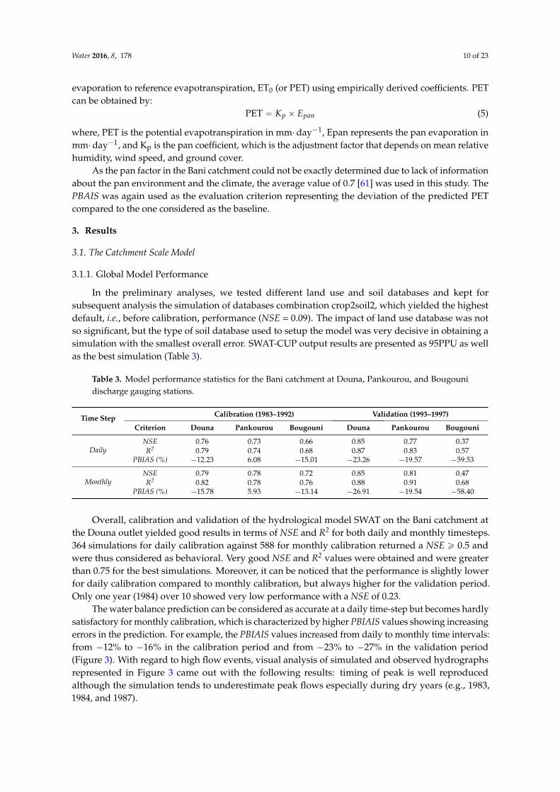
Water 2016, 8, 178 10 of 23
evaporation to reference evapotranspiration, ET0 (or PET) using empirically derived coefficients. PETcan be obtained by:
PET “ Kp ˆ Epan (5)
where, PET is the potential evapotranspiration in mm¨day´1, Epan represents the pan evaporation inmm¨day´1, and Kp is the pan coefficient, which is the adjustment factor that depends on mean relativehumidity, wind speed, and ground cover.
As the pan factor in the Bani catchment could not be exactly determined due to lack of informationabout the pan environment and the climate, the average value of 0.7 [61] was used in this study. ThePBAIS was again used as the evaluation criterion representing the deviation of the predicted PETcompared to the one considered as the baseline.
3. Results
3.1. The Catchment Scale Model
3.1.1. Global Model Performance
In the preliminary analyses, we tested different land use and soil databases and kept forsubsequent analysis the simulation of databases combination crop2soil2, which yielded the highestdefault, i.e., before calibration, performance (NSE = 0.09). The impact of land use database was notso significant, but the type of soil database used to setup the model was very decisive in obtaining asimulation with the smallest overall error. SWAT-CUP output results are presented as 95PPU as wellas the best simulation (Table 3).
Table 3. Model performance statistics for the Bani catchment at Douna, Pankourou, and Bougounidischarge gauging stations.
Time Step Calibration (1983–1992) Validation (1993–1997)
Criterion Douna Pankourou Bougouni Douna Pankourou Bougouni
DailyNSE 0.76 0.73 0.66 0.85 0.77 0.37R2 0.79 0.74 0.68 0.87 0.83 0.57
PBIAS (%) ´12.23 6.08 ´15.01 ´23.26 ´19.57 ´59.53
MonthlyNSE 0.79 0.78 0.72 0.85 0.81 0.47R2 0.82 0.78 0.76 0.88 0.91 0.68
PBIAS (%) ´15.78 5.93 ´13.14 ´26.91 ´19.54 ´58.40
Overall, calibration and validation of the hydrological model SWAT on the Bani catchment atthe Douna outlet yielded good results in terms of NSE and R2 for both daily and monthly timesteps.364 simulations for daily calibration against 588 for monthly calibration returned a NSE ě 0.5 andwere thus considered as behavioral. Very good NSE and R2 values were obtained and were greaterthan 0.75 for the best simulations. Moreover, it can be noticed that the performance is slightly lowerfor daily calibration compared to monthly calibration, but always higher for the validation period.Only one year (1984) over 10 showed very low performance with a NSE of 0.23.
The water balance prediction can be considered as accurate at a daily time-step but becomes hardlysatisfactory for monthly calibration, which is characterized by higher PBIAIS values showing increasingerrors in the prediction. For example, the PBIAIS values increased from daily to monthly time intervals:from ´12% to ´16% in the calibration period and from ´23% to ´27% in the validation period(Figure 3). With regard to high flow events, visual analysis of simulated and observed hydrographsrepresented in Figure 3 came out with the following results: timing of peak is well reproducedalthough the simulation tends to underestimate peak flows especially during dry years (e.g., 1983,1984, and 1987).

Water 2016, 8, 178 11 of 23
Water 2016, 8, 178 12 of 23
the watershed scale. In this case, we focused on available PET and biomass for which there exist regional values.
Table 4. Average annual basin values of precipitation (P), evapotranspiration (ET), potential evapotranspiration (PET), and biomass as SWAT outputs on the Bani catchment.
Period P (mm) ET (mm) PET (mm) a Biomass (ton ha−1)
Agricultural Land Generic
Savannah Forest
Calibration (1983–1992) 960 895 1926 1.18 0.27 3.09
Validation (1993–1997) 1050 975 1925 1.72 0.53 5.51
a Average annual PET estimated by the Hargreaves method (herein used by SWAT).
Figure 3. Simulated and observed hydrographs at Douna station at (a) daily and (b) monthly timesteps along with calculated statistics on calibration and validation periods.
Average annual basin values simulated by the model and described in Section 2.8 are shown in Table 4. The analysis of these values came out with several results. On average, PEThar presented a positive PBIAS of 11% compared with observed PETpen herein equal to 1737 mm and the latter is very close to PETpan, estimated to 1755 mm. These results give a clear indication of overestimation of PET by the SWAT model over the Bani catchment, an overestimation that can be attributed to the Hargreaves method used herein by the model to compute PET.
To further investigate the model’s accuracy, we evaluated predicted biomass values over the calibration/validation period (Table 4) against reported values for the study area. Simulated biomass was on average 4.3 ton·ha−1 for forest and 1.45 ton·ha−1 for agricultural land and both are in the ranges of observed values in the region (the observed biomass ranges between 2–4 and 2–3 ton·ha−1 for forest and cultivated land, respectively [23,62]). Nevertheless, this component is far underestimated for savannah with a simulated value of 0.4 ton ha−1 compared to the observed value which varies between 0.8 and 2 ton·ha−1 [62].
(a)
(b)
Figure 3. Simulated and observed hydrographs at Douna station at (a) daily and (b) monthly timestepsalong with calculated statistics on calibration and validation periods.
3.1.2. Verification of Average Annual Basin Values
Table 4 reports the average annual values of the SWAT model simulated on the Bani catchment.However, there are not available data to enable a full verification of all model outputs at the watershedscale. In this case, we focused on available PET and biomass for which there exist regional values.
Table 4. Average annual basin values of precipitation (P), evapotranspiration (ET), potentialevapotranspiration (PET), and biomass as SWAT outputs on the Bani catchment.
Period P (mm) ET (mm) PET (mm) aBiomass (ton ha´1)
AgriculturalLand Generic Savannah Forest
Calibration (1983–1992) 960 895 1926 1.18 0.27 3.09Validation (1993–1997) 1050 975 1925 1.72 0.53 5.51
a Average annual PET estimated by the Hargreaves method (herein used by SWAT).
Average annual basin values simulated by the model and described in Section 2.8 are shown inTable 4. The analysis of these values came out with several results. On average, PEThar presenteda positive PBIAS of 11% compared with observed PETpen herein equal to 1737 mm and the latter isvery close to PETpan, estimated to 1755 mm. These results give a clear indication of overestimationof PET by the SWAT model over the Bani catchment, an overestimation that can be attributed to theHargreaves method used herein by the model to compute PET.

Water 2016, 8, 178 12 of 23
Table 5. Summary of the SWAT model parameters calibrated on the Bani catchment at Douna on a daily time interval.
Parameter Description Input Calibration Range Calibrated Parameters: BestParameter Value [Range]
Global Sensitivity Analysis
t-Stat p-Value
CN2 SCS runoff curve number II (-) ˘20% ´0.155 [´0.199; 0.102] ´54.03083 0.00000OV_N Manning’s “n” value for overland flow (-) 0.01–30 23.153 [3.061; 29.915] 11.41603 0.00000
SLSUBBSN Average slope length (m) 10–150 149.808 [12.677; 149.924] 8.87352 0.00000ESCO Soil evaporation compensation factor (-) 0.01–1 0.958 [0.768; 0.991] ´6.08880 0.00000
SOL_AWC Available water capacity of the soil layer(mm H2O/mm sol) ˘20% 0.140 [´0.199; 0.197] 2.89864 0.00376
GW_DELAY Groundwater delay (days) 0.0–50 4.938 [0.487; 49.823] 1.81341 0.06980
GWQMN Threshold depth of water in the shallow aquiferrequired for return flow to occur (mm H2O) 0.0–4000 3082.500 [0.043; 3995.710] ´1.51853 0.12891
REVAPMN Threshold depth of water in the shallow aquiferfor “revap” to occur (mm H2O) 0–500 173.709 [0.636; 499.845] ´0.64939 0.51610
RCHRG_DP Deep aquifer percolation fraction (-) 0–1 0.346 [0.001; 0.999] 0.46408 0.64260GW_REVAP Groundwater “revap” coefficient (-) 0.02–0.2 0.190 [0.021; 0.199] ´0.12613 0.89963
SURLAG Surface runoff lag coefficient (-) 0.05–24 20.219 [0.076; 23.878] ´0.07433 0.94075ALPHA_BF* Baseflow alpha factor (d´1) 0.034 0.034 ND ND
* Determined on observed discharges by applying the baseflow filter program. ND: Not Determined.

Water 2016, 8, 178 13 of 23
To further investigate the model’s accuracy, we evaluated predicted biomass values over thecalibration/validation period (Table 4) against reported values for the study area. Simulated biomasswas on average 4.3 ton¨ha´1 for forest and 1.45 ton¨ha´1 for agricultural land and both are in theranges of observed values in the region (the observed biomass ranges between 2–4 and 2–3 ton¨ha´1
for forest and cultivated land, respectively [23,62]). Nevertheless, this component is far underestimatedfor savannah with a simulated value of 0.4 ton ha´1 compared to the observed value which variesbetween 0.8 and 2 ton¨ha´1 [62].
3.1.3. Sensitivity Analysis
There is a wide range of uses for which sensitivity analysis is performed. Based on the12 selected SWAT parameters (ALPHA_BF being fixed), a GSA was used herein for identifying sensitiveand important model parameters in order to better understand which hydrological processes aredominating the streamflow generation in the Bani catchment.
Sensitivity analysis results of 10,000 simulations are summarized in Table 5. The three mostsensitive parameters (CN2, OV_N, and SLSUBBSN) are directly related to surface runoff, reflectingtherefore the dominance of this process on the streamflow generation in the Bani catchment. Processesoccurring at soil level followed at the second position as pointed out by the sensitivity of ESCO andSOL_AWC. Groundwater parameters happened in the last position demonstrating the low contributionof the latter to flows measured at the Douna outlet. The same sensitive parameters were identified bydaily and monthly calibrations with only different ranks for soils parameters (ESCO and SOL_AWC).
3.1.4. Spatial Validation
The results of the spatial validation were divergent according to the location (Figure 4). Forinstance, at Pankourou, the same parameter sets determined at Douna produced a good simulation ona monthly basis (satisfactory for daily validation) whereas predictive uncertainty remained adequateand all met our requirements (NSE > 0.5, P-factor > 0.5 and R-factor < 1). In addition, the water balancewas reasonably predicted at both time steps. In contrast, it has been recorded a complete loss ofmodel performance at Bougouni with unsatisfactory NSE values and more uncertainty related to inputdischarge as expressed by a lower percentage of observed data (P-factor = 0.55 et 0.57 for daily andmonthly validation) inside the 95PPU band (Figure 4). Accordingly, important uncertainty could beattributed to observed discharge at Bougouni.
3.2. The Subcatchment Model
Statistical evaluation results of the subcatchment calibration are presented in Table 3 and timeseries of observed and simulated hydrographs are shown in Figures 5 and 6. Good to very goodperformance was obtained at Pankourou with accurate predictive uncertainty. However, the validationperiod remained unsatisfactorily simulated at Bougouni. A comparative analysis of the catchment andsubcatchment calibration performances came out with the following results:
‚ When calibrated separately, the prediction at Pankourou was slightly better, but greatly improvedat Bougouni compared to when the catchment wide model was applied.
‚ The total uncertainty of the model is smaller at Pankourou (smaller R-factor and larger P-factor)than at the whole catchment, but larger at Bougouni.
‚ The water balance is better simulated at both internal stations compared to the watershed-widewater balance as depicted by smaller PBIAIS values, except always in the validation periodat Bougouni.
‚ The model performance in terms of NSE and R2 was higher at the watershed-wide level than atthe sub-watershed level.
Overall, these results revealed that further calibration at the internal gauging stations wassynonymous with gain of performance at the subcatchment level.

Water 2016, 8, 178 14 of 23
Water 2016, 8, x 15 of 23
3.1.4. Spatial Validation
The results of the spatial validation were divergent according to the location (Figure 4). For instance, at Pankourou, the same parameter sets determined at Douna produced a good simulation on a monthly basis (satisfactory for daily validation) whereas predictive uncertainty remained adequate and all met our requirements (NSE > 0.5, P-factor > 0.5 and R-factor < 1). In addition, the water balance was reasonably predicted at both time steps. In contrast, it has been recorded a complete loss of model performance at Bougouni with unsatisfactory NSE values and more uncertainty related to input discharge as expressed by a lower percentage of observed data (P-factor = 0.55 et 0.57 for daily and monthly validation) inside the 95PPU band (Figure 4). Accordingly, important uncertainty could be attributed to observed discharge at Bougouni.
Figure 4. Spatial validation of the SWAT model on the Bani catchment. The model was turned at Pankourou ((a) daily and (b) monthly time steps) and at Bougouni ((c) daily and (d) monthly timesteps) by using the same behavioral parameter sets determined at the Douna outlet on the period 1983–1992.
3.2. The Subcatchment Model
Statistical evaluation results of the subcatchment calibration are presented in Table 3 and time series of observed and simulated hydrographs are shown in Figures 5 and 6. Good to very good performance was obtained at Pankourou with accurate predictive uncertainty. However, the validation period remained unsatisfactorily simulated at Bougouni. A comparative analysis of the catchment and subcatchment calibration performances came out with the following results:
• When calibrated separately, the prediction at Pankourou was slightly better, but greatly improved at Bougouni compared to when the catchment wide model was applied.
Figure 4. Spatial validation of the SWAT model on the Bani catchment. The model was turned atPankourou ((a) daily and (b) monthly time steps) and at Bougouni ((c) daily and (d) monthly timesteps)by using the same behavioral parameter sets determined at the Douna outlet on the period 1983–1992.
Water 2016, 8, 178 16 of 23
• The total uncertainty of the model is smaller at Pankourou (smaller R-factor and larger P-factor) than at the whole catchment, but larger at Bougouni.
• The water balance is better simulated at both internal stations compared to the watershed-wide water balance as depicted by smaller PBIAIS values, except always in the validation period at Bougouni.
• The model performance in terms of NSE and R2 was higher at the watershed-wide level than at the sub-watershed level.
Overall, these results revealed that further calibration at the internal gauging stations was synonymous with gain of performance at the subcatchment level.
Figure 5. Simulated and observed hydrographs at Pankourou station at (a) daily and (b) monthly time steps along with calculated statistics on calibration and validation periods.
(a)
(b)
Figure 5. Simulated and observed hydrographs at Pankourou station at (a) daily and (b) monthly timesteps along with calculated statistics on calibration and validation periods.

Water 2016, 8, 178 15 of 23
Water 2016, 8, 178 17 of 23
Figure 6. Predicted and measured discharges at Bougouni station at (a) daily and (b) monthly intervals during the calibration and validation periods with their corresponding statistics.
3.3. Model Predictive Uncertainty
In the global model, the predictive uncertainty, as indicated by the P-factor and R-factor, is adequate, though being larger during peak flow and recession periods (reflected by larger 95PPU band). On a daily basis, for instance, 61% of the observed discharge data are bracketed by a narrow 95PPU band depicted by the R-factor < 1 (Table 6). It has been noted that the entire uncertainty band is, however, very large during the year 1984 (Figure 3).
It is important to note the decrease of predictive uncertainty from Douna to Pankourou. In fact, the percentage of observed discharge bracket by 95PPU band has increased to 68%, while the width of the uncertainty band itself has decrease to 0.41 for the daily calibration (Table 6).
Table 6. Predictive uncertainty indices of the SWAT model for the Bani catchment at Douna, Pankourou, and Bougouni discharge gauging stations.
Time Step Calibration (1983–1992) Validation (1993–1997)
Criterion Douna Pankourou Bougouni Douna Pankourou Bougouni
Daily P-factor 0.61 0.68 0.60 0.62 0.63 0.51 R-factor 0.59 0.41 0.57 0.51 0.29 0.35
Monthly P-factor 0.65 0.71 0.58 0.70 0.67 0.55 R-factor 0.65 0.45 0.54 0.55 0.31 0.32
The same trend has been observed for the monthly calibration. At Bougouni, results showed a clear decrease of the uncertainty band (for daily and monthly calibration), but at the expense of bracketing less observed data. For instance, the P-factor and R-factor decreased from 0.65 to 0.58 and from 0.65 to 0.54, respectively, when moving from Douna to Bougouni during the monthly calibration.
Moreover, an increase of the uncertainty band with increasing time step (daily to monthly) has been recorded as depicted by higher R-factor values at Douna and Pankourou (from 0.59 to 0.65 and
(a)
(b)
Figure 6. Predicted and measured discharges at Bougouni station at (a) daily and (b) monthly intervalsduring the calibration and validation periods with their corresponding statistics.
3.3. Model Predictive Uncertainty
In the global model, the predictive uncertainty, as indicated by the P-factor and R-factor, is adequate,though being larger during peak flow and recession periods (reflected by larger 95PPU band). On adaily basis, for instance, 61% of the observed discharge data are bracketed by a narrow 95PPU banddepicted by the R-factor < 1 (Table 6). It has been noted that the entire uncertainty band is, however,very large during the year 1984 (Figure 3).
Table 6. Predictive uncertainty indices of the SWAT model for the Bani catchment at Douna, Pankourou,and Bougouni discharge gauging stations.
Time Step Calibration (1983–1992) Validation (1993–1997)
Criterion Douna Pankourou Bougouni Douna Pankourou Bougouni
Daily P-factor 0.61 0.68 0.60 0.62 0.63 0.51R-factor 0.59 0.41 0.57 0.51 0.29 0.35
Monthly P-factor 0.65 0.71 0.58 0.70 0.67 0.55R-factor 0.65 0.45 0.54 0.55 0.31 0.32
It is important to note the decrease of predictive uncertainty from Douna to Pankourou. In fact,the percentage of observed discharge bracket by 95PPU band has increased to 68%, while the width ofthe uncertainty band itself has decrease to 0.41 for the daily calibration (Table 6).
The same trend has been observed for the monthly calibration. At Bougouni, results showeda clear decrease of the uncertainty band (for daily and monthly calibration), but at the expense ofbracketing less observed data. For instance, the P-factor and R-factor decreased from 0.65 to 0.58 andfrom 0.65 to 0.54, respectively, when moving from Douna to Bougouni during the monthly calibration.

Water 2016, 8, 178 16 of 23
Moreover, an increase of the uncertainty band with increasing time step (daily to monthly) hasbeen recorded as depicted by higher R-factor values at Douna and Pankourou (from 0.59 to 0.65 andfrom 0.41 to 0.45, respectively). However, the uncertainty band was reduced during the validationperiod compared to the calibration period for all the stations (Table 6).
4. Discussion
4.1. Model Performance
In an effort to assess the performance of the SWAT model on the Bani catchment, we calibratedand validated the model at multiple sites on daily and monthly time steps by using measured climatedata. There was no statistically significant difference in model performance among time intervals.Using guidelines given in Moriasi et al. [50], the overall performance of the SWAT model in termsof NSE and R2 can be judged as very good, especially considering limited data conditions in thestudied area. On a monthly basis, we obtained at the Douna outlet a NSE value equal to 0.79 for thecalibration period (0.85 for the validation period). These results are greater than the ones of the studiesby Schuol and Abbaspour [12], and Schuol et al. [14] at the same outlet. Schuol and Abbaspour [12]reported indeed a negative NSE (between ´1 and 0) for the monthly calibration and a value rangingbetween 0 and 0.7 for monthly validation, while Schuol et al. [14] obtained a NSE between 0 and0.70 for both monthly calibration and validation. However, Laurent and Ruelland [23] reported agreater performance (NSE values varying between 0.81 and 0.91 for calibration and validation period,respectively) but on a coarser time step (average annual basis). The water balance is less well simulated,especially for monthly time step with a PBIAIS greater than 25% in absolute value.
The quantified prediction uncertainty is surprisingly satisfactory (Table 6). At the end of thedaily calibration, the model was able to account for 61% of observed discharge data (65% for monthlycalibration) in a narrow uncertainty band. These results are close to the result of Schuol et al. [14] whoestimated the observed discharge data bracketed by the 95PPU between 60% and 80% for monthlycalibration (40% and 60% for monthly validation). However, one explanation that could be attributedto the small uncertainty band we obtained is that model predictive uncertainty derived by GLUEdepends largely on the threshold value to separate “behavioral” from “non-behavioral” parametersets [63,64].
This means, a high threshold value (as in this case) will generally lead to a narrower uncertaintyband [65–67] but this will be achieved at the cost of bracketing less observed data within the95PPU band. In addition, GLUE accounts partly for uncertainty due to the possible non-uniqueness(or equifinality) of parameter sets during calibration and could therefore underestimate total modeluncertainty [68]. For instance, Sellami et al. [69] showed that the GLUE predictive uncertainty bandwas larger and surrounded more observation data when uncertainty in the discharge data wasexplicitly considered. Engeland and Gottschalk [70] demonstrated that the conceptual water balancemodel structural uncertainty was larger than parameter uncertainty. In spite of all the aforementionedlimitations of GLUE, we succeeded in enclosing interestingly most of the observed data within a narrowuncertainty band (the sought adequate balance between the two indices) hence increasing confidencein model results. These are encouraging results showing, on one hand, the good performance ofthe SWAT model on a large Soudano-Sahelian catchment under limited data and varying climateconditions and, on the other hand, the capability of observed climate and hydrological input data ofthis catchment, even though contested, to provide reliable information about hydro-meteorologicalsystems prevailing in the region.
It has been also noted that the model did not perform well during the year 1984 particularly (lowerperformance and larger uncertainty). This loss of performance can be attributed to the disruptionin rainfall-runoff relationship consequence of consecutive years of drought, which has prevailed inthe beginning of the 80s. The over-predicted PET on the Bani catchment could be attributed to theHargreaves method, which could give a greater estimate of PET than it actually is. Ruelland et al. [28]

Water 2016, 8, 178 17 of 23
applied a temperature-based method given by Oudin et al. [71] and provided a similar estimate ofPET (1723 mm) than the values calculated herein by the Penman and pan evaporation methods hencecorroborating our results. These results demonstrated the valuable of pan evaporation measurementsfor estimating PET and that the simple pan evaporation method appears to be suited for application inthe study area and can be used when all the climatic data required by the Penman method are missing.
As far as biomass is concerned, the underestimation of this component in savannah could beexplained by inappropriate specification of all categories in the land use map grid to be modeledby SWAT as savannah or inaccurate savannah characteristics added in the SWAT database, directlyaffecting biomass production such as BIO_E and LAI parameters, among others.
4.2. Impact of Spatial and Temporal Scales on the Model Uncertainty
Results showed that transferring the model parameters from the catchment outlet (Douna) tothe internal gauging stations performs reasonably well only in the case of similarity between donorand target catchments. The case of catchments controlled by Douna and Pankourou gives a clearexample of such physical proximity where precipitation, soil and land use vary smoothly between bothcatchments. However, the SWAT model parameters determined at the outlet could not reproduce wellthe measured discharge at Bougouni mainly due to more significant spatial dissimilarities. Bougouniis indeed situated in a more humid zone and dominated by forest whereas Douna is more arid.Moreover, it has been demonstrated that the individual calibration at subcatchment scale has led toa narrower uncertainty band and more observed discharge data enclosed in it, which is the soughtadequate balance between the two indices. Hence, predictive uncertainty was found to decreasewith decreasing spatial scale. This finding can be attributed to the presence of less heterogeneity inhydrological variables in smaller catchments. These results showed the importance of the calibration ofhydrological models at finer spatial scale to ensure that predominant processes in each subcatchmentare captured, and this is particularly relevant in case of large-area global catchments. Concerningthe effect of temporal scale, we demonstrated that the validation period is characterized by lesspredictive uncertainty as opposed to the calibration period. One explanation that can be given is thefact that 1993-1997 constitutes a more humid period than 1983-1992 and is characterized, therefore,by less variability in precipitation. In contrast, when moving from daily to monthly calibration, theuncertainty of the model, in terms of uncertainty band width, increased. This could be attributedto the cumulative effect of uncertainty in daily discharge data used to compute monthly discharge,resulting therefore in larger monthly uncertainty. Overall, due to decreasing prediction uncertaintywith decreasing spatial and temporal scales, it is germane to develop on the basin a more efficientsystem of hydro-meteorological data collection to account for spatial and temporal variabilities inhydro-meteorological systems prevailing in the region, especially under changing climate and landuse conditions.
4.3. Advance in Understanding of Hydrological Processes
The GSA confirms what has already been reported on and around the Bani catchment about thecontribution of hydrological processes to streamflow generation. In order to better understand theorigin of flows at Kolondieba (a tributary of the Bani River), Dao et al. [72] showed that Groundwatercontribution to the hydrodynamic equilibrium at the outlet of watershed Kolondieba is small and thedirect flow from the soil surface governs the runoff process. This fact can be explained by the doubleimpact of a general impoverishment of shallow aquifers due to reduction in precipitation in WestAfrica in general since the great drought of the 70s as well as a concurrent increase of the recessioncoefficient of the Bani river as demonstrated by Bamba et al. [32] and Mahé [73] with a decrease ofbaseflow contribution to total flow in absolute and relative values as corollary.

Water 2016, 8, 178 18 of 23
4.4. Spatial Performance
The results of different calibration and validation techniques showed varying predictive abilities ofthe SWAT model through scales. Firstly, it can be derived from these findings that model performancein terms of NSE and R2 was higher on the watershed-wide level than on the sub-watershed level.However, this could be attributed to compensation between positive and negative errors of processesoccurring at a larger scale [74,75]. This suggests that calibrating a model only at the basin outletleads to an overconfidence in its performance than at the sub-basin scale. Secondly, individualcalibration of subcatchment processes expectedly improved model accuracy in predicting flows at theinternal gauging stations, due to reducing heterogeneities with downsizing space [76], and is especiallybeneficent while the donor and receiver catchments are substantially different. Finally, predictiveuncertainty appears to decrease with reducing spatial scale, but increases with humidity as shownby the lower performance recorded at Bougouni. The inability of the model to perform during thevalidation period at Bougouni could be attributed to the structure of the validation period which issubstantially different to that of calibration, and is solely composed by average to wet years while incontrast, the occurrence of dry, average, and wet years during the calibration period is noted.
These results have an important role to play in the calibration and validation approaches oflarge-area watershed models and constitutes a first step to model parameter regionalization forprediction in ungauged basins.
Generally speaking, it is well known that in recent decades the Niger River basin has suffered froma serious degradation of its natural resources, which in turn lead to severe environmental issues. To thisend, different agreements and collaborations on water and climate data sharing have been establishedbetween the 9 countries sharing the basin through different national and international programs.Thus, the need to reinforce the existing framework of integrated, coordinated, and sustainable watermanagement strategies in the Bani basin and therefore the Niger River Basin become more urgentthan ever.
Therefore, this study is a step in that long-term direction, where an integrated water managementtool has been developed and validated spatially on the Bani catchment, which allows investigation offuture effects of land use and climate change scenarios on water resources.
5. Conclusions
In this study, the performance of the widely-used SWAT model was evaluated on the Banicatchment using both split-sample and split-location calibration and validation techniques on dailyand monthly intervals. The model was calibrated at the Douna outlet and at two internal stations.Freely available global data and daily observed climate and discharge data were used as inputs formodel simulation and calibration. Calibration, validation, uncertainty, and sensitivity analyses wereperformed with GLUE within SWAT-CUP. Both graphical and statistical techniques were used forhydrologic calibration results evaluation. Evapotranspiration and biomass production outputs wereverified and compared to regional values to make sure these components were reasonably predicted.Sensitivity analysis contributed to a better understanding of the hydrological processes occurring atthe study area.
Final results showed a good SWAT model performance to predict daily as well as monthlydischarge at Douna with acceptable predictive uncertainty despite the poor data density and thehigh gradient of climate and land use characterizing the study catchment. However, the dailycalibration resulted in less predictive uncertainty than the monthly calibration. The performanceof the model is somehow lower at an internal sub-catchments level when the global parameter sets areapplied, especially at the one with higher humidity and dominated by forest. However, subcatchmentcalibration induced an increase of model performance at intermediate gauging stations as well asa decrease of total uncertainty. With regard to predicted PET, this component is overestimated bythe model when the Hargreaves method is applied in that specific region while biomass production

Water 2016, 8, 178 19 of 23
remained low in the savannah land use category. The GSA revealed the predominance of surface andsubsurface processes in the streamflow generation of the Bani River.
Overall, this study has shown the validity of the SWAT model for representing globallyhydrological processes of a large-scale Soudano-Sahelian catchment in West Africa. Given the highspatial variability of climate, soil, and land use characterizing the catchment, additional calibrationis however needed at subcatchment level to ensure that predominant processes are captured in eachsubcatchment. Accordingly, the importance of spatially distributed hydrological measurementsis demonstrated and constitutes the backbone of any type of progress in hydrological processunderstanding and modeling. The calibrated SWAT model for the Bani can be used to assess thecurrent and future impacts of climate and land use change on water resources of the catchment,increasingly necessary information awaited by water resources managers. Knowing this information,a strategy of adaptation in response to the current and future impacts can be clearly proposed andthe vulnerability of the population can therefore be reduced. More widely, this impact study canincrease the transferability of the model parameters from the Bani subcatchment to another ungaugedbasin with some similarities, and then predicting discharge without the need of any measurement.These findings are very useful, especially in West Africa, where many river basins are ungauged orpoorly gauged.
Acknowledgments: Authors are extremely grateful to AGRHYMET for providing the climatic database. Wewould like also to thank Kone Soungalo for climate data on the Ivorian part of the Bani basin and Francois Laurentfor soil and land use databases.
Funding: This study was funded by the German Ministry of Education and Research (BMBF) through theWest African Science Service Centre on Climate Change and Adapted Land Use (WASCAL; www.wascal.org)that supports the Graduate Research Program Climate Change and Water Resources at the University ofAbomey-Calavi. Additional funds were provided by AGRHYMET through the French Global EnvironmentFacility (FFEM/CC) project.
Author Contributions: All authors designed the objectives and methods of the study. J. C. Begou, P. Bazie, andA. Afouda collected the climatological and hydrological datasets required for the model. J. C. Begou, S. Jomaa,S. Benabdallah, and M. Rode conducted the model setup and performed the simulations. All authors analyzedthe obtained data. J. C. Begou prepared the manuscript with contributions from all co-authors. All authors readand approved the final manuscript.
Conflicts of Interest: The authors declare no conflict of interest.
References
1. Pomeroy, J.W.; Spence, C.; Whitfield, P.H. Putting prediction in ungauged basins into practice. In PuttingPrediction in Ungauged Basins into Practice; Canadian Water Resources Association: Ottawa, ON, Canada,2013; pp. 1–12.
2. Sivapalan, M.; Takeuchi, K.; Franks, S.W.; Gupta, V.K.; Karambiri, H.; Lakshmi, V.; Liang, X.; McDonnell, J.J.;Mendiondo, E.M.; O’Connell, P.E.; et al. Iahs decade on predictions in ungauged basins (PUB), 2003–2012:Shaping an exciting future for the hydrological sciences. Hydrol. Sci. J. 2003, 48, 857–880. [CrossRef]
3. Bormann, H.; Diekkrüger, B. Possibilities and limitations of regional hydrological models applied withinan environmental change study in Benin (West Africa). Phys. Chem. Earth Parts A/B/C 2003, 28, 1323–1332.[CrossRef]
4. Kapangaziwiri, E.; Hughes, D.A.; Wagener, T. Incorporating uncertainty in hydrological predictions forgauged and ungauged basins in Southern Africa. Hydrol. Sci. J. 2012, 57, 1000–1019. [CrossRef]
5. Mazvimavi, D.; Meijerink, A.M.J.; Savenije, H.H.G.; Stein, A. Prediction of flow characteristics using multipleregression and neural networks: A case study in Zimbabwe. Phys. Chem. Earth Parts A/B/C 2005, 30, 639–647.[CrossRef]
6. Minihane, M. Estimating mean monthly streamflow in the Lugenda River, Northern Mozambique. In PuttingPrediction in Ungauged Basins into Practice; Canadian Water Resources Association: Ottawa, ON, Canada,2013; pp. 185–196.
7. Ndomba, P.; Mtalo, F.; Killingtveit, A. SWAT model application in a data scarce tropical complex catchmentin Tanzania. Phys. Chem. Earth Parts A/B/C 2008, 33, 626–632. [CrossRef]

Water 2016, 8, 178 20 of 23
8. Nkamdjou, L.S.; Bedimo, J.B. Critique des Donnees Hydrometriques du Bassin du Niger: Rapport Preliminaire;Niger Basin Authority: Niamey, Niger, 2008; p. 28.
9. IPCC. Climate Change 2014: Impacts, Adaptation, and Vulnerability. Part B: Regional Aspects; Barros, V.R.,Field, C.B., Dokken, D.J., Mastrandrea, M.D., Mach, K.J., Bilir, T.E., Chatterjee, M., Ebi, K.L., Estrada, Y.O.,Genova, R.C., et al., Eds.; Cambridge University Press: Cambridge, UK; New York, NY, USA, 2014; p. 688.
10. Wagener, T.; Wheater, H.S.; Gupta, H.V. Rainfall-Runoff Modelling in Gauged and Ungauged Catchments; ImperialCollege Press: London, UK, 2004; p. 332.
11. Amadou, A.; Djibo Abdouramane, G.; Ousmane, S.; Sanda Ibrah, S.; Sittichok, K. Changes to flow regime onthe Niger River at Koulikoro under a changing climate. Hydrol. Sci. J. 2015, 60, 1709–1723.
12. Schuol, J.; Abbaspour, K.C. Calibration and uncertainty issues of a hydrological model (SWAT) applied toWest Africa. Adv. Geosci. 2006, 9, 137–143. [CrossRef]
13. Schuol, J.; Abbaspour, K.C. Using monthly weather statistics to generate daily data in a SWAT modelapplication to West Africa. Ecol. Model. 2007, 201, 301–311. [CrossRef]
14. Schuol, J.; Abbaspour, K.C.; Srinivasan, R.; Yang, H. Estimation of freshwater availability in the West Africansub-continent using the SWAT hydrologic model. J. Hydrol. 2008, 352, 30–49. [CrossRef]
15. Schuol, J.; Abbaspour, K.C.; Yang, H.; Srinivasan, R.; Zehnder, A.J.B. Modeling blue and green wateravailability in Africa. Water Resour. Res. 2008, 44, 1–18. [CrossRef]
16. Sittichok, K.; Gado Djibo, A.; Seidou, O.; Moussa Saley, H.; Karambiri, H.; Paturel, J. Statistical seasonalrainfall and streamflow forecasting for the Sirba watershed, West Africa, using sea surface temperatures.Hydrol. Sci. J. 2014, 61, 1700–1712. [CrossRef]
17. Awotwi, A.; Yeboah, F.; Kumi, M. Assessing the impact of land cover changes on water balance componentsof White Volta Basin in West Africa. Water Environ. J. 2015, 29, 259–267. [CrossRef]
18. Guzinski, R.; Kass, S.; Huber, S.; Bauer-Gottwein, P.; Jensen, I.; Naeimi, V.; Doubkova, M.; Walli, A.; Tottrup, C.Enabling the use of earth observation data for integrated water resource management in Africa with thewater observation and information system. Remote Sens. 2014, 6, 7819–7839. [CrossRef]
19. Sood, A.; Muthuwatta, L.; McCartney, M. A SWAT evaluation of the effect of climate change on the hydrologyof the Volta River Basin. Water Int. 2013, 38, 297–311. [CrossRef]
20. Bossa, A.Y.; Diekkrüger, B.; Giertz, S.; Steup, G.; Sintondji, L.O.; Agbossou, E.K.; Hiepe, C. Modeling theeffects of crop patterns and management scenarios on N and P loads to surface water and groundwater in asemi-humid catchment (West Africa). Agric. Water Manag. 2012, 115, 20–37. [CrossRef]
21. Bossa, A.Y.; Diekkrüger, B.; Igué, A.M.; Gaiser, T. Analyzing the effects of different soil databases on modelingof hydrological processes and sediment yield in Benin (West Africa). Geoderma 2012, 173–174, 61–74.
22. Sintondji, L.O.; Barnabé, Z.; Ahouansou, D.M.; Vissin, W.E.; Agbossou, K.E. Modelling the water balance ofouémé catchment at the savè outlet in Benin: Contribution to the sustainable water resource management.Int. J. AgriSci. 2014, 4, 74–88.
23. Laurent, F.; Ruelland, D. Modélisation à base physique de la variabilité hydroclimatique à l’échelle d’ungrand bassin versant tropical. In Global Change: Facing Risks and Threats to Water Resources, Proceedingsof the sixth world FRIEND conference, Fez, Morroco, 25–29 October 2010; International Association ofHydrological Sciences (IAHS): Wallingford, UK, 2010; pp. 474–484.
24. Ruelland, D.; Ardoin-Bardin, S.; Billen, G.; Servat, E. Sensitivity of a lumped and semi-distributedhydrological model to several methods of rainfall interpolation on a large basin in West Africa. J. Hydrol.2008, 361, 96–117.
25. Masih, I.; Maskey, S.; Uhlenbrook, S.; Smakhtin, V. Assessing the impact of areal precipitation input onstreamflow simulations using the SWAT model. J. Am. Water Resour. Assoc. 2011, 47, 179–195. [CrossRef]
26. Paturel, J.E.; Ouedraogo, M.; Mahé, G.; Servat, E.; Dezetter, A.; Ardoin, S. The influence of distributedinput data on the hydrological modelling of monthly river flow regimes in West Africa. Hydrol. Sci. J. 2003,48, 881–890.
27. Food and Agriculture Organization of the United Nations (FAO). Digital Soil Map of the World and DerivedSoil Properties; Version 3.6; Land and Water Development Division, FAO: Rome, Italy, 2003.
28. Ruelland, D.; Ardoin-Bardin, S.; Collet, L.; Roucou, P. Simulating future trends in hydrological regime of alarge sudano-sahelian catchment under climate change. J. Hydrol. 2012, 424–425, 207–216.

Water 2016, 8, 178 21 of 23
29. Loveland, T.R.; Reed, B.C.; Brown, J.F.; Ohlen, D.O.; Zhu, Z.; Yang, L.; Merchant, J.W. Development of aglobal land cover characteristics database and IGBP DISCover from 1 km AVHRR data. Int. J. Remote Sens.2000, 21, 1303–1330.
30. L’Hote, Y.; Mahé, G.; Some, B.; Triboulet, J.P. Analysis of a sahelian annual rainfall index from 1896 to 2000;the drought continues. Hydrol. Sci. J. 2002, 47, 563–572. [CrossRef]
31. Mahé, G.; Olivry, J.-C.; Dessouassi, R.; Orange, D.; Bamba, F.; Servat, E. Relations eaux de surface-eauxsouterraines d’une rivière tropicale au Mali. Comptes Rendus de l’Académie des Sciences Series IIA Earth Planet.Sci. 2000, 330, 689–692. [CrossRef]
32. Bamba, F.; Mahe, G.; Bricquet, J.P.; et Olivry, J.C. Changements climatiques et variabilite des ressourcesen eau des bassins du haut niger et de la cuvette lacustre. XIIèmes journees hydrologiques de l’orstom 1996,10–11, 1–27.
33. Ruelland, D.; Guinot, V.; Levavasseur, F.; Cappelaere, B. Modelling the longterm impact of climatechange on rainfall-runoff processes over a large sudano-sahelian catchment. In New Approaches toHydrological Prediction in Data Sparse Regions, Proceedings of the Symposium HS.2 at the Joint Conventionof The International Association of Hydrological Sciences (IAHS) and The International Association ofHydrogeologists (IAH), Hyderabad, India, 6–12 September 2009; IAHS: Wallingford, UK, 2009; pp. 59–68.
34. Arnold, J.G.; Srinivasan, R.; Muttiah, R.S.; Williams, J.R. Large area hydrologic modeling and assessmentpart i: Model development. J. Am. Water Resour. Assoc. 1998, 34, 73–89. [CrossRef]
35. Winchell, M.; Srinivasan, R.; di Luzio, M.; Arnold, J.G. Arcswat Interface for SWAT. 2012 User’s Guide; Soil andWater Research Laboratory, USDA Agricultural Research Service: Temple, TX, USA, 2013; p. 459.
36. Arnold, J.G.; Kiniry, J.R.; Srinivasan, R.; Williams, J.R.; Haney, E.B.; Neitsch, S.L. Soil and Water AssessmentTool Input/Output Documentation: Version 2012; Texas Water Resources Institute Technical Report: CollegeStation, TX, USA, 2012; Volume TR-439.
37. Neitsch, S.L.; Arnold, J.G.; Kiniry, J.R.; Williams, J.R. Soil and Water Assessment Tool Theoretical Documentation:Version 2009; Technical Report No. 406; Texas Water Resources Institute Texas: College Station, TX,USA, 2011.
38. Bouraoui, F.; Benabdallah, S.; Jrad, A.; Bidoglio, G. Application of the SWAT model on the Medjerda RiverBasin (Tunisia). Phys. Chem. Earth Parts A/B/C 2005, 30, 497–507. [CrossRef]
39. Ouessar, M.; Bruggeman, A.; Abdelli, F.; Mohtar, R.H.; Gabriels, D.; Cornelis, W.M. Modellingwater-harvesting systems in the arid south of Tunisia using SWAT. Hydrol. Earth Syst. Sci. 2009, 13,2003–2021. [CrossRef]
40. World Meteorological Organization (WMO). WMO-No.100. Guide to Climatological Practices, 3rd ed.; WMO:Geneva, Switzerland, 2011.
41. Boisramé, G. WGN Excel Macro. Available online: http://swat.Tamu.Edu/software/links/ (accessed on25 April 2016).
42. USGS Hydrosheds. Available online: http://hydrosheds.cr.usgs.gov/dataavail.php (accessed on26 April 2016).
43. Waterbase. Available online: http://www.waterbase.org/resources.html (accessed on 26 April 2016).44. FAO. Available online: http://www.fao.org/geonetwork/srv/en/main.home (accessed on 26 April 2016).45. Nash, J.E.; Sutcliffe, J.V. River flow forecasting through conceptual models part I—A discussion of principles.
J. Hydrol. 1970, 10, 282–290. [CrossRef]46. Moussa, R.; Chahinian, N.; Bocquillon, C. Distributed hydrological modelling of a mediterranean
mountainous catchment—Model construction and multi-site validation. J. Hydrol. 2007, 337, 35–51.[CrossRef]
47. Robson, B.J.; Dourdet, V. Prediction of sediment, particulate nutrient and dissolved nutrient concentrationsin a dry tropical river to provide input to a mechanistic coastal water quality model. Environ. Model. Softw.2015, 63, 97–108. [CrossRef]
48. Abbaspour, K.C. SWAT-Cup 2012: SWAT Calibration and Uncertainty Programs—A User Manual; Eawag, SwissFederal Institute of Aquatic Science and Technology: Duebendorf, Switzerland, 2014; p. 106.
49. Beven, K.; Binley, A. The future of distributed models: Model calibration and uncertainty prediction.Hydrol. Process. 1992, 6, 279–298. [CrossRef]

Water 2016, 8, 178 22 of 23
50. Moriasi, D.N.; Arnold, J.G.; van Liew, M.W.; Bingner, R.L.; Harmel, R.D.; Veith, T.L. Model evaluationguidelines for systematic quantification of accuracy in watershed simulations. Trans. ASABE 2007, 50,885–900. [CrossRef]
51. Arnold, J.G.; Allen, P.M.; Muttiah, R.; Bernhardt, G. Automated base flow separation and recession analysistechniques. Ground Water 1995, 33, 1010–1018. [CrossRef]
52. Arnold, J.G.; Allen, P.M. Automated methods for estimating baseflow and ground water recharge fromstreamflow records. J. Am. Water Resour. Assoc. 1999, 35, 411–424. [CrossRef]
53. Betrie, G.D.; Mohamed, Y.A.; van Griensven, A.; Srinivasan, R. Sediment management modelling in the BlueNile Basin using SWAT model. Hydrol. Earth Syst. Sci. 2011, 15, 807–818. [CrossRef]
54. Van Griensven, A.; Meixner, T.; Grunwald, S.; Bishop, T.; Diluzio, M.; Srinivasan, R. A global sensitivityanalysis tool for the parameters of multi-variable catchment models. J. Hydrol. 2006, 324, 10–23. [CrossRef]
55. Zhang, X.; Srinivasan, R.; Liew, M.V. Multi-site calibration of the SWAT model for hydrologic modeling.Trans. ASABE 2008, 51, 2039–2049. [CrossRef]
56. Arnold, J.G.; Moriasi, D.N.; Gassman, P.W.; Abbaspour, K.C.; White, M.J.; Srinivasan, R.; Santhi, C.;Harmel, R.D.; Griensven, A.V.; Liew, M.W.V.; et al. SWAT: Model use, calibration, and validation.Trans. ASABE 2012, 55, 1491–1508. [CrossRef]
57. Abbaspour, K.C.; Johnson, C.A.; van Genuchten, M.T. Estimating uncertain flow and transport parametersusing a sequential uncertainty fitting procedure. Vadose Zone J. 2004, 3, 1340–1352. [CrossRef]
58. Hargreaves, G.L.; Hargreaves, G.H.; Riley, J.P. Agricultural benefits for Senegal River Basin. J. Irrig. Drain.Eng. 1985, 111, 113–124. [CrossRef]
59. Allen, R.G.; Pereira, L.S.; Raes, D.; Smith, M. Crop Evapotranspiration-Guidelines for Computing Crop WaterRequirements-FAO Irrigation and Drainage Paper 56; Food and Agriculture Organization of the United Nations(FAO): Rome, Italy, 1998.
60. Doorenbos, J.; Pruitt, W.O. Guidelines for Predicting Crop Water Requirements, Irrigation and Drainage Paper 24;Land and Water Development Division, FAO: Rome, Italy, 1975; p. 179.
61. Brouwer, C.; Heibloem, M. Irrigation Water Management: Training Manual No. 3; Food and AgricultureOrganization of the United Nations (FAO): Rome, Italy, 1986.
62. Coulibaly, A. Profil Fourrager (Mali); Food and Agriculture Organization of the United Nations (FAO):Rome, Italy, 2003.
63. Mantovan, P.; Todini, E. Hydrological forecasting uncertainty assessment: Incoherence of the GLUEmethodology. J. Hydrol. 2006, 330, 368–381. [CrossRef]
64. Montanari, A. Large sample behaviors of the generalized likelihood uncertainty estimation (GLUE) inassessing the uncertainty of rainfall-runoff simulations. Water Resour. Res. 2005, 41, 1–13. [CrossRef]
65. Blasone, R.-S.; Madsen, H.; Rosbjerg, D. Uncertainty assessment of integrated distributed hydrologicalmodels using GLUE with Markov chain Monte Carlo sampling. J. Hydrol. 2008, 353, 18–32. [CrossRef]
66. Viola, F.; Noto, L.V.; Cannarozzo, M.; La Loggia, G. Daily streamflow prediction with uncertainty inephemeral catchments using the GLUE methodology. Phys. Chem. Earth Parts A/B/C 2009, 34, 701–706.[CrossRef]
67. Xiong, L.; O’Connor, K.M. An empirical method to improve the prediction limits of the GLUE methodologyin rainfall—Runoff modeling. J. Hydrol. 2008, 349, 115–124. [CrossRef]
68. Yen, H.; Wang, X.; Fontane, D.G.; Harmel, R.D.; Arabi, M. A framework for propagation of uncertaintycontributed by parameterization, input data, model structure, and calibration/validation data in watershedmodelling. Environ. Model. Softw. 2014, 54, 211–221. [CrossRef]
69. Sellami, H.; Vanclooster, M.; Benabdallah, S.; La Jeunesse, I. Assessment of the SWAT model predictionuncertainty using the GLUE approach a case study of the Chiba catchment (Tunisia). In Modeling, Simulationand Applied Optimization (ICMSAO), Proceedings of the 5th International Conference, Hammamet, Tunisia,28–30 April 2013; Institute of Electrical and Electronics Engineers (IEEE): New York, NY, USA, 2013; pp. 1–6.
70. Engeland, K.; Gottschalk, L. Bayesian estimation of parameters in a regional hydrological model.Hydrol. Earth Syst. Sci. 2002, 6, 883–898. [CrossRef]
71. Oudin, L.; Hervieu, F.; Michel, C.; Perrin, C.; Andréassian, V.; Anctil, F.; Loumagne, C. Which potentialevapotranspiration input for a lumped rainfall-runoff model? Part 2 towards a simple and efficient potentialevapotranspiration model for rainfall-runoff modelling. J. Hydrol. 2005, 303, 290–306. [CrossRef]

Water 2016, 8, 178 23 of 23
72. Dao, A.; Kamagate, B.; Mariko, A.; Seguis, L.; Maiga, H.B.; Goula Bi, T.A.; Savane, I. Deconvolution of theflood hydrograph at the outlet of watershed kolondieba in the south of Mali. Int. J. Eng. Res. Appl. 2012,2, 1174–1181.
73. Mahé, G. Surface/groundwater interactions in the Bani and Nakambe rivers, tributaries of the Niger andVolta Basins, West Africa. Hydrol. Sci. J. 2009, 54, 704–712. [CrossRef]
74. Cao, W.; Bowden, W.B.; Davie, T.; Fenemor, A. Multi-variable and multi-site calibration and validation ofSWAT in a large mountainous catchment with high spatial variability. Hydrol. Process. 2006, 20, 1057–1073.[CrossRef]
75. Wellen, C.; Kamran-Disfani, A.-R.; Arhonditsis, G.B. Evaluation of the current state of distributed watershednutrient water quality modeling. Environ. Sci. Technol. 2015, 49, 3278–3290. [CrossRef] [PubMed]
76. Daggupati, P.; Yen, H.; White, M.J.; Srinivasan, R.; Arnold, J.G.; Keitzer, C.S.; Sowa, S.P. Impact of modeldevelopment, calibration and validation decisions on hydrological simulations in West Lake Erie Basin.Hydrol. Process. 2015, 29, 5307–5320. [CrossRef]
© 2016 by the authors; licensee MDPI, Basel, Switzerland. This article is an open accessarticle distributed under the terms and conditions of the Creative Commons Attribution(CC-BY) license (http://creativecommons.org/licenses/by/4.0/).