Embed Size (px)
Citation preview
UNIVERSITÁ DEGLI STUDI DI PADOVA
DIPARTIMENTO DI INGEGNERIA DELL’INFORMAZIONE
TESI DI LAUREA TRIENNALE IN INGEGNERIA BIOMEDICA
EXPERIMENTAL VALIDATION OF XSENS INERTIAL SENSORS DURING CLINICAL
AND SPORT MOTION CAPTURE APPLICATIONS
Relatore: Prof. Petrone Nicola
Correlatore: Eng. Giubilato Federico
Correlatore: Marcolin Giuseppe, PhD
Laureando: Cognolato Matteo
ANNO ACCADEMICO 2011/2012


Ai miei cari,
per il continuo e sentito sostegno.
Ad Anita,
senza lei, queste pagine
non sarebbero state scritte.

All trademarks and copyrights are property of their respective owners.

Contents
PREFACE
CHAPTER 1
1.1 Motion Capture 1
1.1.1 Optical Systems 3
1.1.2 Mechanic Systems 5
1.1.3 Magnetic Systems 8
1.1.4 Hybrid Systems 8
1.2 Terminology and conventions 9
CHAPTER 2
2.1 Rotation and Orientation Matrix 11
2.1.1 Basic Rotation Matrices 12
2.1.2 Composition of Rotation Matrices 13
2.1.3 Rotation Matrix Property 14
2.2 Euler Angles 14
2.3 Cardan Angles 15
2.4 Euler “aerospace” Angles 16
2.5 Protocols in literature 18
CHAPTER 3
3.1 Introduction of Xsens technology 23
3.2 Xsens coordinate systems 24
3.2.1 Orientation Output Modes 25
3.2.2 Orientation Reset 26
3.2.2.1 Arbitrary Alignment 26

3.2.2.2 Heading Reset 27
3.2.2.3 Object Reset 28
3.2.2.4 Alignment Reset 29
3.2.3 MT Manager Xsens Software 30
3.3 Considerations about the use of Xsens 30
3.4 Angles definition and conventions 30
CHAPTER 4
4.1 Preliminary considerations 35
4.2 Preliminary tests 36
4.2.1 Battery life test 36
4.2.2 Magnetic field test 37
4.2.3 Pilot ski tests at the Cermis ski area 39
4.2.4 Reset and angular velocity test 45
4.2.5 Gait analysis test 47
4.2.6 Treadmill test 54
4.2.7 Starting blocks test 59
4.3 Considerations about the preliminary tests 61
CHAPTER 5
5.1 Reset method 63
5.2 Comparison between Xsens and optoelectronic system 64
5.3 Matlab software to perform comparison 66
5.4 Validation tests 67
5.4.1 Electrogoniometer test 67
5.4.2 2nd gait analysis test 70
5.4.3 Test of intensive care bed 75

CHAPTER 6
6.1 Joint anatomical axes method 81
6.1.1 Basic movements 82
6.2 Matlab software to calculate rotation axes 83
6.3 Validation test 85
CHAPTER 7
7.1 Conclusions 89
7.2 Future developments 91
CHAPTER 8
8.1 Ringraziamenti 93
8.2 Bibliography 94
8.3 Webography 95


PREFACE
Motion analysis aims to objectively measure body segments movement (kinematics), ground
reaction forces and joint motion (kinetics) as well as muscles activity (electromiograpy). This
discipline has primarly two areas of application: clinical and sport. In the first one motion
analysis can be employed for example in the diagnosis of gait kinematics and kinetics
alterations, in the monitoring of the rehabilitation after injuries or surgeries course but also for
prosthesis and orthoses evaluation. Sport applications are referred to the functional evaluation
of specific aspects of the performance as well as to optimize the training process.
Motion analysis can be performed with several instrumentations which differ for
invasiveness, accuracy and costs. Furthermore, considering the technology of these systems, 4
categories can also be defined: optical, mechanical, magnetic and hybrid. Nowadays
stereophotogrammetric system is the most employed in biomechanical laboratories: it is
considered the golden standard for its accuracy even if it presents some limitations regarding
the subject preparation, the indoor employment and the operating volume due to the number
of cameras.
The interest on Inertial hybrid sensors is growing both considering entertainment applications
but also biomechanical ones as for example ergonomic and sport measurements. The main
advantage of such instruments is the outdoor employment with no limit of operating volume.
In this way it is possible to record real movements in ordinary environment.
Therefore the first aim of the present work was to evaluate the accuracy of the inertial system
MTw developed by Xsens Technologies in clinical and sport applications. The followed
approach was to compare technical frames of both MTws and optoelectronical system . The
second aim was to define the anatomical rotation axes to obtain the most important data in
clinical application: the anatomical angles calculated by joint coordinates system.


1
CHAPTER 1
Introduction
1.1 Motion Capture
Motion Capture is a discipline that studies the human body movement, in order to have an
objective and accurate measurement of :
• body segments movements (kinematics)
• ground reaction forces and joint moments (kinetics)
• electrical muscle activation signal (ElectroMyoGraphy)
Motion Capture is defined as the procedure of recording movements of objects or persons,
therefore it has several area of application, that will be listed in what follows:
I. Clinical applications: in the prosthetic field, both structural design and
characterisation; for movement control and rehabilitation; as well as analysis of
balance system, to control and have a deeper knowledge of pathophysiology of the
skeletal and locomotor apparatus.
II. Sports applications: to increase athletes performance preventing injuries with a
qualitative analysis identifying harmful movements that have to avoided during
training.
III. Ergonomic applications: analysis of human body movements can give the possibility
to create devices with more comfortable and useful design, right to biomechanical
rules.
IV. Entertainment applications: to create animated films or video games with more natural
movements and actions.
V. Other applications: virtual reality, robotic etc.

2
Motion tracking started as a photogrammetric analysis, conducted by Eadweard Muybridge in
1870 – 1880, who proved that a horse can have all four hooves lifted off the ground while
galloping. Later Muybridge also conducted a human movements studies. Etienne-Jules Marey
has been the first person to analyze human and animal motion with video in the end of XIX
sec, he also invented a “chronophotographic gun ” which could take 12 consecutive frames
per second.
Fig 1: Marley’s photographic gun
In 1931 Harold E. Edgerton invented ultra-high-speed and stop-action photography, called
stroboscopic photography. This technology can record images at high speed and results are
more similar to a video rather than a photo, it's natural with this devices to obtain more details
than a single picture and, indeed the cinematography quickly became the principal MoCap
system, although it had a very low accuracy and slow data elaboration. The turning point was
the introduction of digital technology which it lets an automatic and very fast data elaboration
by using calculator, moreover, thanks to this new technology, new MoCap system had been
created; nowadays, the best of these systems can measurement the movements in real time,
with an accuracy less than 0.5 mm.
A Motion Capture system can be assembled in different way, using various technology; it's so
possible to define four approaches to realize a MoCap system:
• Optical systems
• Mechanic systems
• Inertial systems
• Hybrid systems
MoCap system created by one of this approaches, has characteristics linked on the technology
used, that should be valued case to case.
At this moment, the optical system, called optoelectronic system, is the most accurate and
used MoCap system for analysis of movement.

3
1.1.1 Optical Systems
Optical systems are based on photography or video-recording, using different technologies
approaches and methods. The most simple and fast optical system for MoCap is the 2D
cinematography system: consist in a video-recording with a camera and a computer
processing. The second step allows:
o link frames with background matching
o define the size of a known object on the movement plane
o draw remarkable points' track
o calculate absolute and relative angles between body segments
o calculate angular or linear velocity
Fig 2: Long Jump © Dartfish
The next step is cinematography the 3D system, that consist of a collection of video data from
multiple commercial cameras, which enables, after data interpolation by a software
processing, to obtain 3D data of markers. This technique has the same approach as the
optoelectronic system, but it is performed by commercial cameras, involving less accuracy
and less sample rate than optoelectronic system. The main advantage is the possibility to
perform analysis directly on the competition field.
A new 3D video motion capture system is formed only by a video data, without markers or
sensors. The human body is recognized by a special computers algorithms that analyze
multiple real time video data. This method is often used by a entertainment applications, first
of all in video games area; for example the commercial Microsoft device Kinect can
recognize gamers body (with a RGB camera and IR-camera for defined the depth) and this
allows to have a “gamers controller”. This method is used to move animated characters: the
human body movements processed by a software, are the input arguments of a graphical
animated software; in this way the virtual figures will do the same movements of the human
characters.

4
The most used and accurate system at today for MoCap, is the optoelectronic system; it's
compound by infra red cameras, infra red strobes, active or passive markers, three axes frame
with markers for calibration and model defined by operator.
Optoelectronic system needs six or more cameras to perform analysis (the number can change
due to study and accuracy level required) because for calculate 3D position of markers every
single marker must be recorded by two or more cameras. Every camera can identify the
direction between optical camera's centre and where markers reflects the infra red on the
sensor. Knowing the direction it can obtain the straight line through this two points and, the
intersection of two straight derived by two cameras, allows to identify the 3D marker position.
The markers are small spheres and it can be active or passive: active markers generates
different colours’ light, in this way the cameras can identify single marker, however this type
of markers needs power supply; the second one are covered by a refractive material, that
reflect infra-red produced by strobes, nevertheless in this case for identify single markers it's
necessary to have static markers position and define a "position model". Performing an
optoelectronic recording, needs specific setup steps: first in all the cameras must be placed
around the volume of calibration, in hexagonal way (if there are 6 cameras), trying to avoid
alignment of cameras. During this phase the system detects the global system of reference,
physically determined by a three axes frame with markers, placed in the centre of the volume
of calibration. After the calibration, for every camera the orientation is calculated, as well as
the position, the focal length, the optical centre position and the distortion parameters. All of
this information are necessary to perform 3D reconstruction. The calibration must be done for
a volume proportional with the act to study, because if the volume is too large, the accuracy
will be minor, however if the volume is too small, the act couldn't be recorded in total. 6
Passive markers must be placed on the subject following the position model defined, so it's
possible to identify every single marker by its position. This is fundamental for data
reconstruction step. In the analysis data step, every body segment with markers is represented
by a rigid body (is assumption like the segment's bone), from which is possible to obtain
physiological and anatomical movements. It's very important to minimize every other
movement of markers, due to muscle and skin effect, because only if this hypothesis is
verified, it is possible approximate a body segment like a rigid body. In the human body there
are some points really near at bones processes, where there aren't muscle bundles which can
be activated during movements, this points are calls "Anatomical landmarks". These are the
preferred locations of markers to verified the hypothesis before exposed.
To identify a body segment a group of markers (usually 2 or 3 markers) is needed and it
allows to define the reference system linked to that body segment, with which it's possible to
5
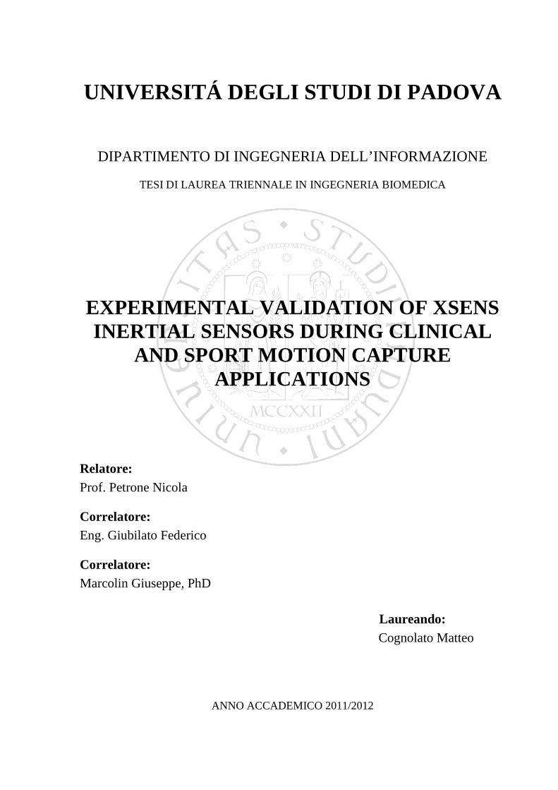
obtain the reconstruction of the movements of the body with respect to the laboratory
reference system (set by calibration step) or with respect to another body segment.
Fig 3: Example of markers application
Fig 4: Example of optoelectronic model
1.1.2 Mechanic Systems
One of the first systems used for human movements analysis was electrogoniometers, which
are a device is able to measure angle between two segments. Before wireless connection, the
biggest defect of this devices was wires interfered with subject movements, however at today
the principal limits of this product are low accuracy and encumbrance on the subject's body.
The electronic evolution, in particular with Micro Electro Mechanical Systems (MEMS),
allowed to create new and smaller sensors, some of which find application for create MoCap
sensors. The most important sensors for analysis of movements sector are accelerometers and
gyroscopes:7
� Accelerometer is an electromechanical device that measures acceleration force, both
static and dynamic. A basic accelerometer consisted of two fundamental parts: a case

6
that will be attacked to the object whose necessary measuring acceleration, and a
seismic mass suspended by a spring, fixed on the case. When object is accelerated, due
to this motion, the spring contract and shorten itself following seismic mass
movements which are proportional to acceleration; knowing the inertia and the
displacement position of mass, it is possible calculate the acceleration (this job is done
by a different sensor that differences the kind of accelerometer: strain gauges,
piezoresistive, piezoelectrical, laser, capacitive..). If 3 accelerometers are arranged like
a X-Y-Z frame, it becomes a 3-dimensional sensor which can measure accelerations in
every space directions. MEMS accelerometers are created using Silicon and, between
all, the ones which use capacitive effects have excellent characteristics. Difference of
capacitor can be caused by a variation of one of this three parameters:
d
AC mεε 00 =
ɛm is the permittivity of the material between two armors, A is the area of them and d
the distance between them. Typical MEMS accelerometers is composed of seismic
mass with plates attached with springs to fixed plates by a mechanical suspension.
This two plates formed the capacitors. Every movements of proof mass causes a
change in capacity which is proportional to the acceleration.
Known mathematical and physics knowledge allows to obtain velocity and position
starting by acceleration.
Fig 5: Detail of a typical MEMS accelerometer
Fig 6: ADXL 320 accelerometer
� Gyroscopes are a devices which can measure or maintain the orientation using the law
of maintenance of angular moment (angular moment of a system is constant if the
result of eternal forces applied to the system is null). This devices tends to maintain its
axle oriented in a fixed direction, regardless of rotations of its frame. A basic
conceptual gyroscope can be made with a rotor (disk or wheel) insert in a gyroscope

7
frame, when the rotor is rotating, its spin tend to maintain it parallel to itself, doesn't
let change its orientation.
As accelerometer, gyroscopes is product with MEMS technology in different type:
vibrating ring gyroscope, macro laser ring gyroscope, piezoelectric plate ring
gyroscope, fiber optic gyroscope and, at last, tuning fork gyroscope which is one of
the most widely use gyroscope. All MEMS gyroscope take advantage of the Coriolis
effect: a moving mass M with v velocity, rotating in a reference frame at angular
velocity ω affected by a force:
ω×= MvF 2
Tuning fork gyroscope is composed by two masses that are built in such a way as to
oscillate with the same intensity but in opposite directions. When rotated, is generated
a Coriolis force that it is bigger when mass is further away from the spin, this creates
an orthogonal vibration that can be detected by different methods.
Fig 7: The first working prototype of the Draper
Lab gyroscope Fig 8: Example of a modern gyroscope
Usually, this two devices are used together because accelerometer’s accuracy is limited;
unfortunately, the accuracy of these sensors is still lower than standard for MoCap systems.
Another mechanical device invented for MoCap area which implements new technologies, are
optical fiber system: this technology allows to create flexibility sensors for evaluate bending
angles. Optical fiber sensors allows freedom of movements, thanks to flexibility of fiber, it
can place on a human subject obtaining in output 3D movements of a human skeleton. These
devices are versatile and easy to use, however, also in this case, the major limitation consists
of a low accuracy; anyhow optical fiber are usually used for didactical and entertainment
applications.

8
1.1.3 Magnetic Systems
Magnetic sensors represent other important devices employed in the MoCap field.
They exploit the property of magnetic field to identify position of sensors and its movements,
this system is composed by a low-frequency transmitter source and sensors which must be
placed on subject’s body segments. The transmitter generate three perpendicular (one to each
other) magnetic fields for every measurement cycle and this is possible because the
transmitter are formed by three perpendicular coils crossed in sequence by the current. Each
3D magnetic sensor can measure strength of those fields which is proportional to the distance
between sensor and source, besides both sensors and transmitter calculates positions of each
sensor from the nine output data of magnetic field strength per sensor. This devices have two
main problems: magnetic fields decrease in power rapidly, for this reason there is a maximum
distance between sensors and transmitter; also the second problem is linked to magnetic field
property, in fact it is very sensible to ferromagnetic materials which can create disturbances,
decreasing the accuracy of the measurement. Magnetic sensors have a peculiarity: they don’t
suffer from “problems of visibility”, human body in fact is crossed by magnetic fields used
and this allows to have not dark points during movements. Another important characteristic is
the constant accuracy of this devices, they can calculate position and orientation with the
same accuracy (if the magnetic field power sensing by the sensors is constant).
1.1.4 Hybrid Systems
Hybrid systems are new MoCap approach, these devices implements more than one MoCap
systems previously exposed, they trying to integrate advantages of systems of which they are
composed and, at the same time, decrease, or, if it is not possible, don’t increase, the systems'
limits. There are several types of hybrid systems, all of them with different characteristics. An
example is hybrid system formed by inertial and magnetic systems, which can be measure
three dimensional position and orientation of all body segments in real time, linking inertial
and magnetic systems property.

9
1.2 Terminology and conventions
“Anatomical position” is the universal starting position for describing movements and, in this
position, three motion planes can be
defined:
o Median/Saggital plane
o Frontal/Coronal plane
o Horizontal/Transverse plane
To define respective position about
structure, there are exactly terms:
proximal, meaning nearer, and distal,
which means more distance, both
respect to origin of anatomical of
interest part (for the arts is the attack
on the body); for example, greater
trocanther is proximal and
medial/lateral epicondyle is distal.
Like position, also movements must be
described with a specific terminology:
Fig 9: anatomical position
o Flexion is the movement that decrease angle between share joint
o Extension is the movement which increase angle between share joint
o Adduction means approaching a movable body parts (such as the leg) to the median
plane
o Abduction is the opposite movement of adduction
o Intra rotation is a movement from lateral to medial
o Extra rotation is the opposite motion of intra rotation

10
11
CHAPTER 2
References
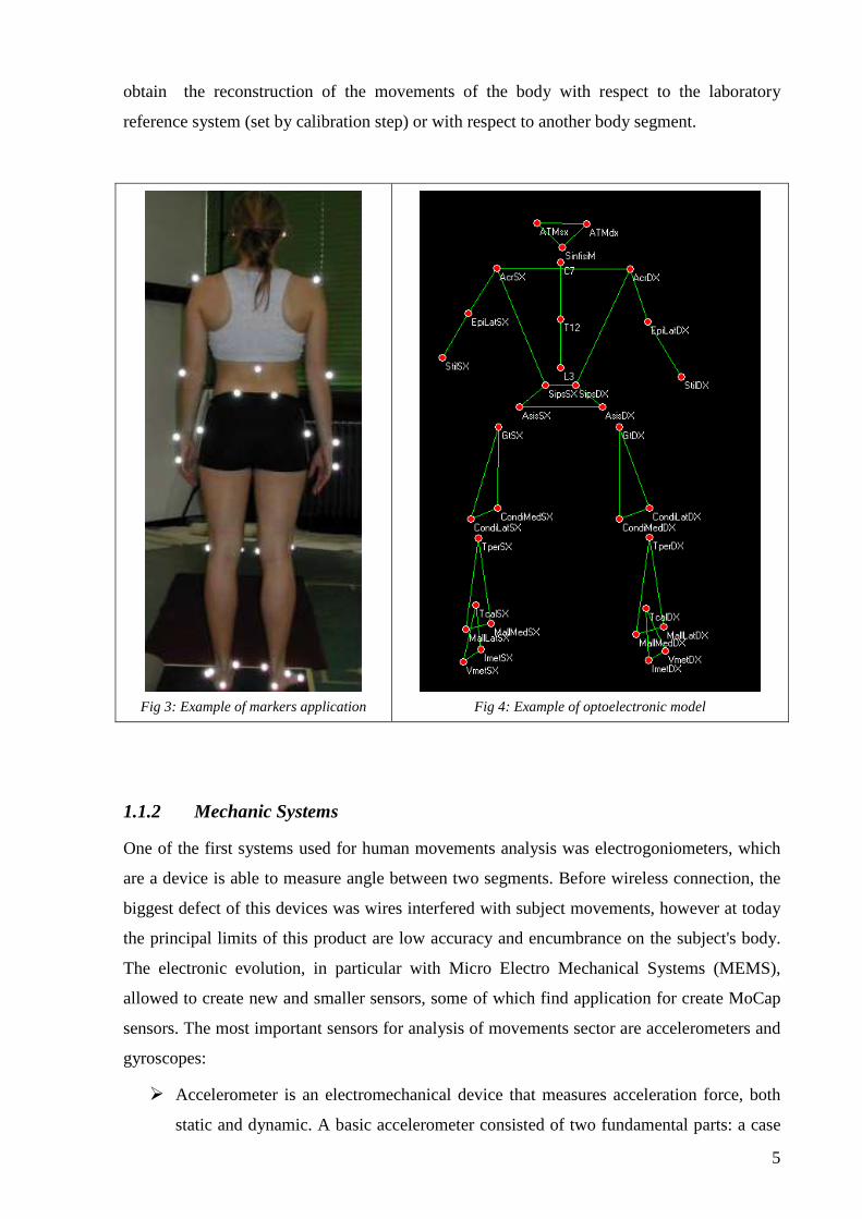
2.1 Rotation and Orientation Matrix
Rotation and orientation matrix are basic algebraic means used to perform rotations in
Euclidean space. A rigid body B is a collection of point in the three dimensional space,
bounded by following relation
( ) ( ) ttPtP ji cos=− Bji ∈∀ ,
which imposes that the distance of two body’s arbitrary points must be constant during time.
The rigid body configurations, is more efficiently defined by rotations and orientations of a
system of reference, that defined the orientation matrix, of the body which refers to a fixed
one; for this reason rotation and orientation matrix are fundamental algebraic operators which
allows to define rigid body configurations, respect other frame of reference defined in the
space.
Orientation matrix having for columns the director
cosines of zyxrrr
,, unit vectors in the SoR1 system:
=)cos()cos()cos(
)cos()cos()cos(
)cos()cos()cos(
zZyZxZ
zYyYxY
zXyXxX
Ro
In general, considering two systems of reference SoR1
[ ]1111 ,,, zyx eeeorrr
and SoR2 [ ]2222 ,,, zyx eeeorrr
(defined by
centre and three unit vectors) having the same centre O
( )21 oo ≡ , and an arbitrary point P in the space, the
X
Z
x
Y
z
yr
xr
zr
SoR1
SoR2
y

12
coordinates of P in both SoR1 and SoR2 are given by projection of the vector OP in the two
systems of reference:1
=
=
=
2
2
212
2
2
2
1,21,21,2
1,21,21,2
1,21,21,2
1
1
1
1
z
y
x
R
z
y
x
eeeeee
eeeeee
eeeeee
z
y
x
C
zzzyzx
yzyyyx
xzxyxx
rrrrrr
rrrrrr
rrrrrr
=
=
=
1
1
121
1
1
1
2,12,12,1
2,12,12,1
2,12,12,1
2
2
2
2
z
y
x
R
z
y
x
eeeeee
eeeeee
eeeeee
z
y
x
C
zzzyzx
yzyyyx
xzxyxx
rrrrrr
rrrrrr
rrrrrr
where C1 are the coordinates of P with respect to the SoR1 and C2 are with respect to the SoR2
system, 21R is the rotation matrix that allows to transform the P point coordinates from the
SoR2 system to SoR1 system and 12R is the one that expresses the SoR1 coordinates in the
SoR2 ones.
In other words, the rotation matrix has the director cosines of zyxrrr
,, unit vectors in the SoR1
system for columns:
=)cos()cos()cos(
)cos()cos()cos(
)cos()cos()cos(
zZyZxZ
zYyYxY
zXyXxX
Rj
which expressing the orientation of the SoR2 with respect to the SoR1, around a joint O.
2.1.1 Basic Rotation Matrices
When there is a rotation around a single axis, it is defined by a basic rotation matrix about
one single axis; obviously it can define three basic rotation matrices:
( )
−=)cos()sin(0
)sin()cos(0
001
αααααxR
1 This notation is used for scalar product: θcos, vuvu
rrrr =
13
−=
)cos(0)sin(
010
)sin(0)cos(
)(
ββ
βββyR
( )
−=
100
0)cos()sin(
0)sin()cos(
γγγγ
γzR
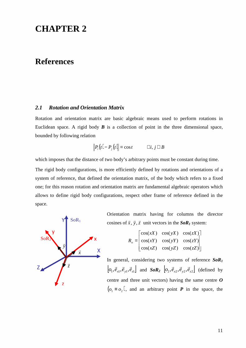
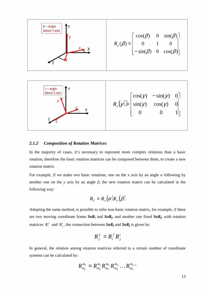
2.1.2 Composition of Rotation Matrices
In the majority of cases, it’s necessary to represent more complex relations than a basic
rotation, therefore the basic rotation matrices can be composed between them, to create a new
rotation matrix.
For example, if we make two basic rotations, one on the x axis by an angle α following by
another one on the y axis by an angle β, the new rotation matrix can be calculated in the
following way:
( ) ( )βα yxT RRR =
Adopting the same method, is possible to refer non-basic rotation matrix, for example, if there
are two moving coordinate frame SoRi and SoRj, and another one fixed SoRf, with rotation
matrices fiR and i
jR , the connection between SoRf and SoRj is given by:
ij
fi
fj RRR =
In general, the relation among rotation matrices referred to a certain number of coordinate
systems can be calculated by:
13
4
2
3
1
2
1 −= n
nn
mm
mm
mm
mm
mm RRRRR K
14
2.1.3 Rotation Matrix property
Initially, when the two systems are coincident, the rotation matrix is the unitary matrix I.
Also, it could be also demonstrate that an arbitrary rotation matrix is orthogonal, in fact
( ) IRR mn
Tmn = ; this means that inverse rotation matrix is equal to the transposed one:
( ) ( )Tmn
mn RR =−1
.
This is a very useful property because it allows to obtain the inverse rotation matrix simply
calculating the inverse (or the transposed) of the rotation matrix:
( ) ( )Tmn
mn
nm RRR == −1
Another characteristic of rotation matrix, is the commutative property only for simply rotation
around the same axis, in case of multiple rotation about different axes the commutative
property doesn’t subsist. Therefore, the sequence whereby basic rotation matrix are multiplied
among them involves different results, in particular:
• Given any basic rotation matrix R, post-multiplication by R corresponds to rotations
around moving axes x-y-z
( ) ( ) ( )γβα zyxo RRRRxyz
=
• Given any basic rotation matrix R, pre-multiplication by R corresponds to rotations
about fixed axes X-Y-Z
( ) ( ) ( )αβγ XYZo RRRRZYX
=
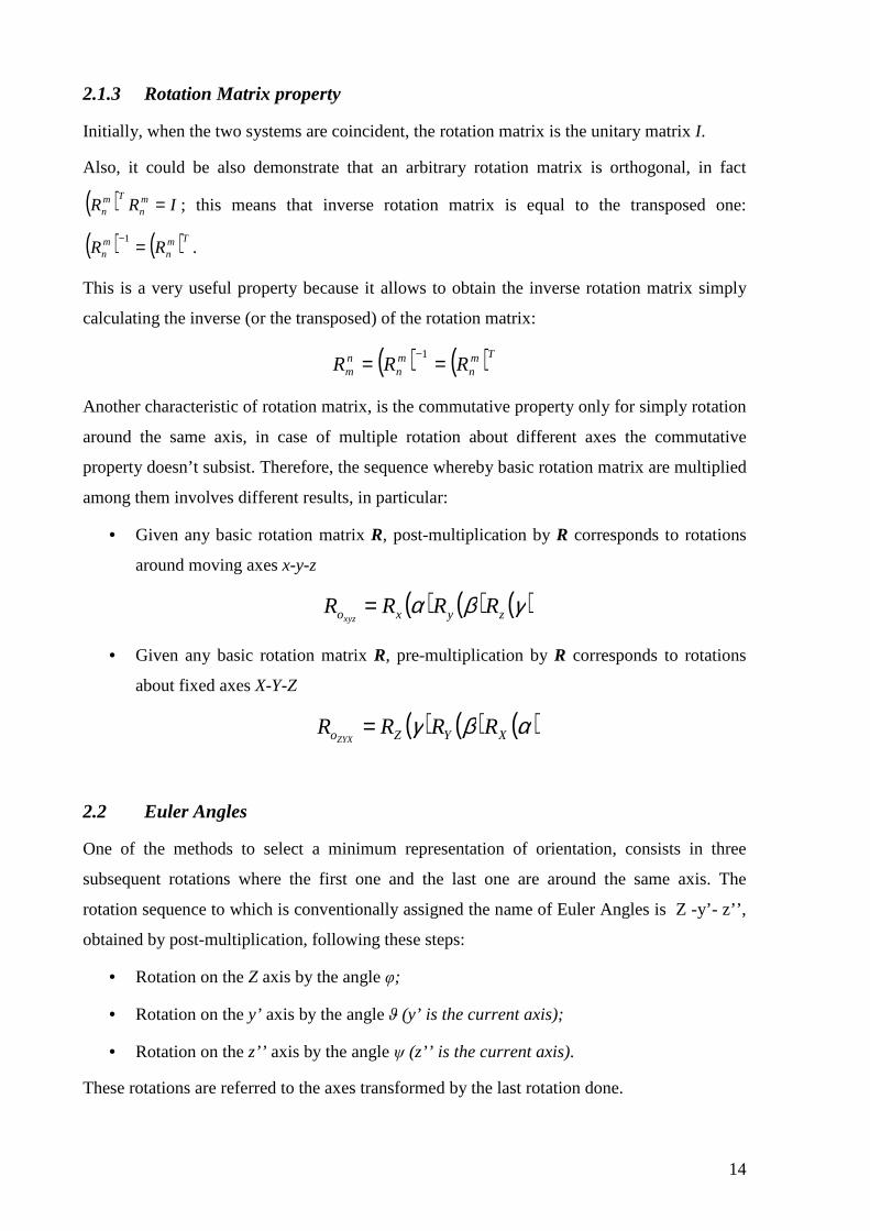
2.2 Euler Angles
One of the methods to select a minimum representation of orientation, consists in three
subsequent rotations where the first one and the last one are around the same axis. The
rotation sequence to which is conventionally assigned the name of Euler Angles is Z -y’- z’’,
obtained by post-multiplication, following these steps:
• Rotation on the Z axis by the angle φ;
• Rotation on the y’ axis by the angle ϑ (y’ is the current axis);
• Rotation on the z’’ axis by the angle ψ (z’’ is the current axis).
These rotations are referred to the axes transformed by the last rotation done.

15
2.3 Cardan Angles
Another method consists of a sequence of rotations around each of three axes. Generally, the
Cardan angles are obtained by a sequence Z - x’- y’’ (avoiding gimbal lock 2) on these
different moving axes by post-multiplication:
( ) ( ) ( )βαγ '''''' yxzo RRRRyZx
=
Ro is obtained by post-multiplication of three basic rotation matrices, with Z -x’-y’’ rotation
sequence:
( ) ( ) ( )
−
−
−==
=ββ
ββ
ααααγγ
γγβαγ
cos0sin
010
sin0cos
cossin0
sincos0
001
100
0cossin
0sincos
'''
333231
232221
131211
''' yxZo RRR
rrr
rrr
rrr
RyZx
−−++−−
=βααβα
βαγβγαγβαγβγβαγβγαγβαγβγ
coscossinsincos
cossincossinsincoscossinsincoscossin
cossinsinsincoscossinsinsinsincoscos
The three Cardan angles correspond to subsequent rotations that bring the SoR1 to overlap to
the SoR2:
1. Rotation of γ about the Z axis (Z ≡ z’);
2. Rotation of α about the current x axis (x’ ≡ x’’ );
3. Rotation of β about the current y axis (y’’ ≡ y’’’ );
4. The x’’’- y’’’ – z’’’ is corresponding to the SoR2.
2 Gimbal lock is defined as the loss of one degree of freedom due to the alignment of two spin

16
Having the γ, α and β angles values, the relative orientation matrix is obtained by replacing
values in the Ro final matrix.
The other solution is the inverse approach: given the rotation matrix, the three γ, α and β
angles can be obtained by trigonometric solutions of suitable terms. The trigonometric
solutions for Cardan angles are:
( )32arcsinr=α
−=
33
31arctanr
rβ
−=
22
12arctanr
rγ
2.4 Euler “aerospace” Angles
Euler "aerospace" angles, called in this way because they are frequently used in aerospace
field, defined the RPY convention, where R is "Roll" , P is "Pitch" and Y is "Yaw". This
convention is more interpretable if it is referred of an airplane with a system of reference
where the z axis is placed along the fuselage, the y axis is placed along the wingspan and the
x axis in according to the right hand rule.
The method consist in three consecutive rotations executed with a X – Y – Z (Roll – Pitch –
Yaw) sequence about the three perpendicular axes of the original frame:
• Rotation of ψ angle around Z axis;
• Rotation of θ angle around Y axis (the original one);
• Rotation of ϕ angle around X axis (the original one).
The three rotations listed before are obtained from rotation matrices which pre-multiplication
the preceding rotation:
x=x’’’ y=y’’=y’’’
z=z’’’
X
Y
Z=z’
x’=x’’
z’’
α β
γ
α γ
β
SoR1
SoR2

17
( ) ( ) ( )φθψ XYzo RRRRXYZ
=
Euler “aerospace” angles correspond to the Z - y' - x'' Cardan angles sequence.
The matrix obtained by pre-multiplication of the three basic matrices, in according to Euler
“aerospace” method, is:
( ) ( ) ( ) =
−
−
−==
=φφφφ
θθ
θθψψψψ
φθψcossin0
sincos0
001
cos0sin
010
sin0cos
100
0cossin
0sincos
333231
232221
131211
XYzo RRR
rrr
rrr
rrr
RXYZ
−+−+
++−=
φθφθθφθψφψφθψφψθψ
φθψφψφθψφψθψ
coscossincossin
cossinsinsincossinsinsincoscoscossin
cossincossinsinsinsincoscossincoscos
Even in this case there are two approaches, the direct and the inverse: the first one allows to
obtain the rotation matrix XYZoR substituting the values of ψ, θ and ϕ angles; with the inverse
approach the three angles ψ, θ and ϕ values are obtained by trigonometric solution of suitable
terms. The trigonometric solutions for Euler “aerospace” angles are:
=
33
32arctanr
rφ ( )31arcsinr−=θ
=
11
21arctanr
rψ
The three Euler “aerospace” angles correspond to subsequent rotations that bring the SoR1 to
overlap to the SoR2:
1. Rotation of ϕ about the fixed X axis (Ex: 30°)
2. Rotation of θ about the fixed Y axis (Ex:80°)
3. Rotation of ψ about the fixed Z axis (Ex: -30°)
4. The x’’’ – y’’’ – z’’’ is corresponding to the SoR2
18
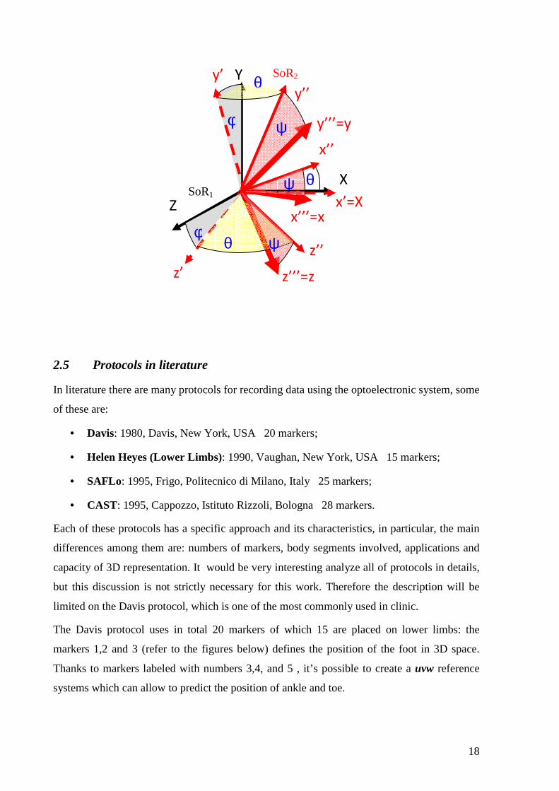
2.5 Protocols in literature
In literature there are many protocols for recording data using the optoelectronic system, some
of these are:
• Davis: 1980, Davis, New York, USA 20 markers;
• Helen Heyes (Lower Limbs): 1990, Vaughan, New York, USA 15 markers;
• SAFLo: 1995, Frigo, Politecnico di Milano, Italy 25 markers;
• CAST: 1995, Cappozzo, Istituto Rizzoli, Bologna 28 markers.
Each of these protocols has a specific approach and its characteristics, in particular, the main
differences among them are: numbers of markers, body segments involved, applications and
capacity of 3D representation. It would be very interesting analyze all of protocols in details,
but this discussion is not strictly necessary for this work. Therefore the description will be
limited on the Davis protocol, which is one of the most commonly used in clinic.
The Davis protocol uses in total 20 markers of which 15 are placed on lower limbs: the
markers 1,2 and 3 (refer to the figures below) defines the position of the foot in 3D space.
Thanks to markers labeled with numbers 3,4, and 5 , it’s possible to create a uvw reference
systems which can allow to predict the position of ankle and toe.
x’’
y’’
z’’
X
Y
Z x’=X
y’
z’
θ
θ
x’’’=x
y’’’=y
z’’’=z
φ
φ θ
ψ
ψ
ψ
SoR1
SoR2

19
Fig 10: Markers position on David protocol (anterior view)
Fig 11: Markers position on David protocol (posterior view)
Fig 12: Markers to define 3D calf position
Fig 13: Markers to define foot position.
The uvw reference systems can be used in specific prediction equations (based on
anthropometric dimensions data) to estimate the positions of anatomical points. The Davis
protocol defines also the segment reference frames positions and orientation: they must be
embedded at the centres of gravity of each body segment with a defined orientation for each

20
axis. The method used to calculate relative anatomic angles, is easier to explain with an
example, as left knee’s rotation axis:
There are three separate ranges of
motion:
1. Flexion and extension take place
about the mediolateral axis of
the left Thigh (Z2);
2. internal and external rotation
take place about the longitudinal
axis of the left calf (X4);
3. abduction and adduction take
place about an axis that is
perpendicular to both Z2 and X4.
Note that these three axes do not form a
right-handed triad, because Z2 and X4
are not necessarily at right angles to one
another.
Fig 14: Axes of rotation for the left knee
The corresponding abduction and adduction unit vector is calculated by vector product of
corresponding unit vectors of Z2 and X4 axes:
42
42
xz
xzy AdAb rr
rr
r
⊗⊗
=−
Anatomical joint angles can be calculated thanks to the formulas of the inverse approach
applied at the Euler resolution angles. Moreover is possible calculate Euler angle for segment
absolute orientation, even in this case is more simple explaining this with an example as
define orientation of the right calf’s reference frame relative to the global system of reference
XYZ:

21
The three angular degrees of freedom (or Euler
angles ϕRcalf, θRcalf, and ψRcalf) defining the
orientation of the right calf’s reference axes (xRcalf,
yRcalf, and zRcalf) relative to the global reference
system XYZ. Note that the calf’s CG has been
moved to coincide with the origin of XYZ.
The three Euler angle rotations take place in the
following order:
(a) ϕRcalf about the Z axis;
(b) θRcalf about the line of nodes;
(c) ψRcalf about the zRcalf axis.
Fig 15: Coordinate system of the right calf

22

23
CHAPTER 3
Xsens Technology
3.1 Introduction of Xsens technology
Xsens Technologies is a developer of 3D motion tracking products, based on inertial sensors
manufactured with MEMS technology. The Xsens product used in these work is the MTw™
is a miniature wireless inertial measurement unit (IMU). It is a small, lightweight and
completely wireless 3D motion tracker, formed by 3D linear accelerometers, 3D rate
gyroscopes, 3D magnetometers and a barometer (for pressure measurement). This product
returns 3D orientation, acceleration, angular velocity, static pressure and earth-magnetic field
intensity. The MTw™ has an embedded processor that handles sampling, calibration,
buffering and strap down integration of the inertial data, it also controls the wireless network
protocol for data transmission. Wireless transmission is created and maintained by the (patent-
pending) Awinda™ radio protocol. This feature can handle up to 32 MTw™ IMU and the
accuracy of 3D motion tracking is maintained in case of a temporary loss of transmission
data. Awinda™ station, using the Awinda™ radio protocol, enables an initially data sampling
at 1800 Hz but this involves too many data for wireless transmission and, generally, a too
heavy computational load on a typical host device. Therefore the MTw™ processor down-
sampling data at 600 Hz, with Step Down Integration (SDI) the data is transmitted to the
Awinda station and, finally, on the PC using USB interface.
Fig 16: Motion traker Xsens MTw™
Fig 17: the Xsens Awinda station

24
The sample rate can be chosen by the user but it depends from the numbers of linked sensors:
the user can choose a sampling rate up to 150 Hz using one MTw™, with more than one
sensor, the sampling rate will proportionally decrease according to the number of devices (e.g.
with 5 connected MTw™ the maximum sample rate is 75Hz). Awinda station allows to use
up to two input synchronization signals and two output synchronization signals, moreover
user can decide which type of synchronization to implements in according to his systems.
Another important characteristic of Awinda station is that power supply is only needed for
charging MTw™, for updating its firmware and to reactivate the MTw™ if it has been
switched off at the end of last utilization. A fundamental feature is that for Xsens MTw
product, the USB power is enough for wireless communication, both for measurement and
recording, indeed it’s worth remembered that each MTw™ has a LiPo battery with a capacity
of 220mAh which ensures 2.5-3.5 hours of run-time 3.
The body straps are a quick and comfortable solution for fixing the MTws™ to the
subject/patient’s body. Each MTw™ is equipped with a special click mechanism that allows
quick and safe connection to the strap.
Fig 18: MTw™ click mechanism
Fig 19: MTw™ click-in body straps
3.2 Xsens coordinate systems
Each MTw™ has a right handed fixed coordinate system, that defines the sensor coordinate
frame S (refer to the figure below). This frame is aligned with the sensor's external box but
the real reference is inside and, of course, this may cause an error and a loss of accuracy.
Moreover the alignment between the coordinate system S and the bottom of the MTw™’s box
is guaranteed less within than 3°. Another problem of the inertial sensors in the orthogonality
of the reference system’s axes, but regarding Xsens MTw™ the non-orthogonality is less than
0.1°. In default conditions each MTw™ returns angles between the coordinate system S and
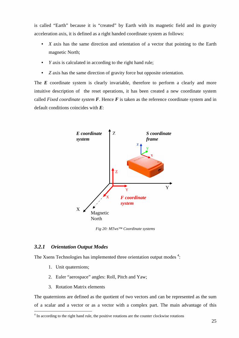
the “Earth” coordinate system E, with E as reference coordinate system. E coordinate frame
3 MTw™ User Manual data
25
is called “Earth” because it is “created” by Earth with its magnetic field and its gravity
acceleration axis, it is defined as a right handed coordinate system as follows:
• X axis has the same direction and orientation of a vector that pointing to the Earth
magnetic North;
• Y axis is calculated in according to the right hand rule;
• Z axis has the same direction of gravity force but opposite orientation.
The E coordinate system is clearly invariable, therefore to perform a clearly and more
intuitive description of the reset operations, it has been created a new coordinate system
called Fixed coordinate system F. Hence F is taken as the reference coordinate system and in
default conditions coincides with E:
Fig 20: MTws™ Coordinate systems
3.2.1 Orientation Output Modes
The Xsens Technologies has implemented three orientation output modes 4:
1. Unit quaternions;
2. Euler “aerospace” angles: Roll, Pitch and Yaw;
3. Rotation Matrix elements
The quaternions are defined as the quotient of two vectors and can be represented as the sum
of a scalar and a vector or as a vector with a complex part. The main advantage of this 4 In according to the right hand rule, the positive rotations are the counter clockwise rotations
X
Y
Z
Magnetic North
E coordinate system
z y
x
S coordinate frame
X
Y
Z
F coordinate system

26
representation is the absence of singularity: on the contrary this problem is present in the
Euler “aerospace” angles and in the rotation matrix representations (in this last case it is
possible to avoid singularity with a particular angle resolution).
The Euler “aerospace” angles mode, returns three angles called Roll, Pitch and Yaw following
the theory explained in the 2.4 paragraph.
The third representation is the rotation matrix elements: as output there are the entries r ij
[ ]3,1, ∈∀ ji that make up the matrix. Following the theory explained in the 2.4 paragraph is
possible to calculate the Euler "aerospace" angles after reconstructing the matrix starting from
the entries in output.
Each of these data, independently of its representation, is returned at every sample.
3.2.2 Orientation Reset
The default settings of the MTw™ can sometimes be strictly, therefore four different
orientation reset were implemented by Xsens. These reset procedures to set different reference
coordinate systems distinguished by the E coordinate system. The reset can be performed for
all sensors or for a selected sensor, therefore this option leaves the user free to decide if and
which reset to perform for each sensor.
3.2.2.1 Arbitrary Alignment
The first type of reset is called Arbitrary Alignment, used to change the sensor coordinate
system S in another known coordinate system. For example, should it be necessary to obtain
in output data referred to a given object coordinate system, using the Arbitrary Alignment is
sufficient to create a rotation matrix OSR which changes the sensor coordinate system S into
the object coordinate system O:
( )TFO
FS
OS RRR =
When this reset is applied, orientation data are given between the object coordinate frame O
(obtained from the changed sensor coordinate frame) and the Fixed coordinate system F.

27
3.2.2.2 Heading Reset
The second type of reset is called “Heading Reset”: it is useful when it is necessary to change
the S coordinate system while keeping Z axis pointing upward and varying only the X axis
direction.
After the Heading Reset, the F coordinate system is changed in a new Fixed frame called F’
characterized by:
• X axis pointing in the same direction of the X axis of the selected Xsens sensor
• Y axis in according to right hand rule
• Z axis pointing upwards (parallel and opposite to gravity)
An important factor to know is that the Heading Reset, both the orientation and magnetic data
will be returned with respect to F’ and the first output data will be:
Roll = previous value Pitch = previous value Yaw = 0°
The returned angles identifying the rotations needed to take F’ to overlap to S.
Fig 21: Stages of Heading Reset
28
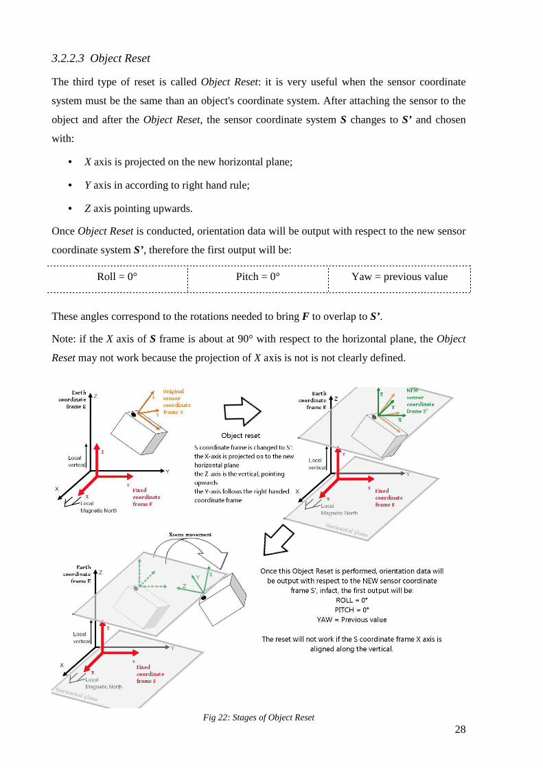
3.2.2.3 Object Reset
The third type of reset is called Object Reset: it is very useful when the sensor coordinate
system must be the same than an object's coordinate system. After attaching the sensor to the
object and after the Object Reset, the sensor coordinate system S changes to S’ and chosen
with:
• X axis is projected on the new horizontal plane;
• Y axis in according to right hand rule;
• Z axis pointing upwards.
Once Object Reset is conducted, orientation data will be output with respect to the new sensor
coordinate system S’, therefore the first output will be:
Roll = 0° Pitch = 0° Yaw = previous value
These angles correspond to the rotations needed to bring F to overlap to S’.
Note: if the X axis of S frame is about at 90° with respect to the horizontal plane, the Object
Reset may not work because the projection of X axis is not is not clearly defined.
Fig 22: Stages of Object Reset

29
3.2.2.4 Alignment Reset
The fourth type of reset is called Alignment Reset and it is the most complete reset of MTw™.
It combines the Object Reset and the Heading Reset in a single time. When the Alignment
Reset is performed, both to S and F coordinate systems are changed in the new S’ and F’
coordinate systems. The first change is done due to the Object Reset and the second due to the
Heading Reset. After the Alignment Reset is performed, orientation data will be output with
respect to the new Fixed coordinate system F’ , and output angles represent the rotation
needed for bringing F’ to overlap S’. The first output after the Alignment Reset is:
Roll = 0° Pitch = 0° Yaw = 0°
Fig 23:Stages of Alignment Reset
These reset could make more adaptable and comfortable using the Xsens MTw™: however,
at the beginning, these reset were not at all intuitive to use because the user manual had a very
poor description of this argument not very clear, in particular for the used notations.

30
3.2.3 MT Manager Xsens Software
The MT Manager is the software that manages connections between Awinda station and
MTws™ and also it visualizes, records and extracts data from MTw™. This software also
allows to perform reset, to select the output orientation mode and the data that will be output
by the software. Moreover the MT Manager performs real time 3D visualisation of:
orientation data (Roll, Pitch and Yaw angles or MTw™ position in the 3D space), and both
inertial and magnetic data (acceleration, angular velocity and magnetic field intensity).
Xsens Technologies has developed the MTw™ Software Development Kit (SDK) that gives
full access to all data and configurations of the MTw™.
3.3 Considerations about the use of Xsens
One of the most important targets of motion analysis is recording the skeleton’s movements,
with the minor possible disturb possible. And other movement, like the skin and muscle
contraction effects, are considered artefacts. The optoelectronic system uses reflective
markers to identify movements, and these markers are placed on “anatomical landmarks”
where skin and muscle artifact are minimum. With respect to the MTws™ positions, for
obvious reasons, it’s impossible to place them on “anatomical landmarks”, therefore in each
recording sessions there will be skin and muscle effects. It is possible to define the best points
to place body straps with MTws™, like the wrist for forearm movements and the lateral side
of to Shank when considering the lower leg movements: but these are simple considerations
to avoid large artefacts due, for example to the calf muscles.
Other artefacts can be due to body straps movements: markers are attached to the body with
biocompatible tape. However MTs are positioned thanks to the straps and, to avoid slippage
during movements, they have, on the interior side, two antislip bands. Despite these solutions,
body straps movements or slippage may be present, and it is necessary to consider a possible
error due to these effects.
3.4 Angles definitions and conventions
In this work, different typologies of angles will be considered: the BTS optoelectronic system
uses Cardan angles where as the Xsens uses the Euler “aerospace” angles, as well as both
technical and physiological angles will be introduced. For this reason, an angle’s conventions
has been adopted to make data analysis simpler and more clear.

31
The first definition adopted concerns the difference between Xsens which adopt Euler
“aerospace” angles and Optoelectronic BTS system which uses Cardan angles:
• Euler “aerospace” angles adopted from Xsens, will be indicated with uppercase
notation:
Φ = Roll Θ = Pitch Ψ = Yaw
• Cardan angles used by Optoelectronic BTS system, will be indicated with lowercase
notation:
ϕ= Roll θ = Pitch ψ = Yaw
By after adopting this convention is possible to identify the typology of angles and what is the
system to which they are referred.
During the tests it a particular posture was used, called physiological reference position
which identify the standing position of the subject. Moreover some angles with particular
property, both technical and physiological were defined:
1. Reset angle: this angle is used during Xsens reset to obtain a defined orientation of the
X axis with respect of the horizontal plane;
2. Static angles: these are output angles referred to the physiological reference position
(static position);
3. Segment angles: by this definition angles detected by Xsens during movements and
referring to the physiological reference position are indicated. They will be indicated
with one subscript identifying the segment that has generated the angles (e.g. ΦT, Θ T,
Ψ T are Roll, Pitch and Yaw angles calculated between Thigh and the physiological
reference position);
4. Segment to Segment angles: these angles are calculated by MTw™ or the
optoelectronic system between two body segments (e.g. movements of Shank with
respect to Thigh). They will be indicated with two subscripts identifying two
segments, between which are calculated these angles (e.g. φ TS, θTS, ψTS are Roll, Pitch
and Yaw Thigh to Shank Cardan angles and Φ ST, Θ ST, ΨST are Shank to Thigh Euler
“aerospace” angles);
5. Joint angles: by this definition physiological/anatomical angles are indicated. They
must be calculated about coordinate system that must be based on bones' movements,
called joint coordinate systems. In this work, the joint angles will be indicated with a
single subscript to identify the joint to which these angles are referred.

32
Fig 24: Static angles
Fig 25:Segment angles
Fig 26:Segment to Segment angles
Fig 27: Joint angles
The Segment to Segment angles and the Joint angles curves recorded during a session trend,
strictly depends on the reference coordinate system. In the gait analysis, if the Shank
coordinate system is taken as reference, the rotations that is coordinate system has to do to
coincident with the Thigh's coordinate system are the angles values returned; on the contrary,
if when the Thigh is taken as reference, its coordinate system will be the moving one.

33
Obviously, for this reason, the plots of the obtained graphs corresponding shell be of opposite
sign, because the coordinate systems rotations are the same but performed in opposite
direction.
In this work, the coordinate system that return the angles in the standard physiological
conventions will be always taken as reference.

34

35
CHAPTER 4
Pilot tests
4.1 Preliminary considerations
The aims of this work is to understand the MTws™ operation and to try developing, a
method for performing the best recording of motions; parallel to this, to create a software to
analyze the data is also an objective. The aims can be schematized with the four targets of this
work:
1. To create a method for performing motion capture and motions analysis with MTw™
developed by Xsens Technologies;
2. To evaluate the accuracy of Xsens when compare to optoelectronic systems;
3. To use the Xsens angular velocity data for calculating the joint's axis of movement
during single motions (e.g. flex-extension or intra-extra rotation) and defining a joint
anatomical coordinate frame;
4. To develop a software for analyzing and processing the data.
Regarding the first target, it was necessary to decide whether to perform a reset, or to use the
default coordinate system (Earth) as reference system. After a long set of tests, it was decided
to perform the Alignment Reset in a novel way that was named “Alignment Reset Pack”: this
reset is performed after have positioned the MTws™ closer to each other, to form a “pack”
(stack up).
The “Alignment Reset” with a "pack" configuration resulted more convenient for two
reasons:
• after performing an “Alignment Reset Pack”, each MTw™ has the same new
coordinate system S’ and it will refer to the same new reference frame F’ ;
• When the MTws™ are placed on the subject/patient’s body in the physiological
reference position, the angles obtained between this position and the sensors reset
position, named as Static angles, give information about how sensors were placed on
36
the body. These angles can also give information about the static position of the
subject/patient, and can highlight postural disorders.
Regarding the second aim of the study, it could be considered the most important, because the
optoelectronic system is nowadays the most used system in clinical and sport area when
performing motion analysis. This system is very accurate and, nowadays, is considered the
golden standard for the analysis of motion.
Regarding the third target, the data analysis step will be fully explained in the 6.1 paragraph.
These theoretical considerations need to be verified by preliminary tests.
4.2 Preliminary tests
Preliminary tests were necessary for deciding which hypothesis were wrong. They allowed
the resolution of problems and improve the methods.
4.2.1 Battery life test
To program a field test, the real time of discharge of battery is a fundamental variable:
therefore a test for evaluating the discharge time of MTws™ was performed. This test was
made following the worst case: this is when all sensors working in acquisition mode. The test
was performed with sensors that had different percentage of initial charge. Thanks to this
differences was possible to determine if different initial charge may have affected the
discharge rate, evaluating the slopes of discharge curves.
During the tests, also the discharge time of the netbook’s battery (that should have been
lasting longer than the MTws™) was evaluated. How it’s possible to note on the figure 28,
only the curve of the 438 sensor had a lower slope than the others: this means that discharge
time speed is independent from starting charge.
Moreover, time discharge time difference between 438 and 440 sensor was about 10%.

37
Fig 28: MTws™ discharge time
Finally the approximate battery life in normal conditions, during acquisition was estimated
between 2.30 – 2.45 hours from an initial 100% charge state.
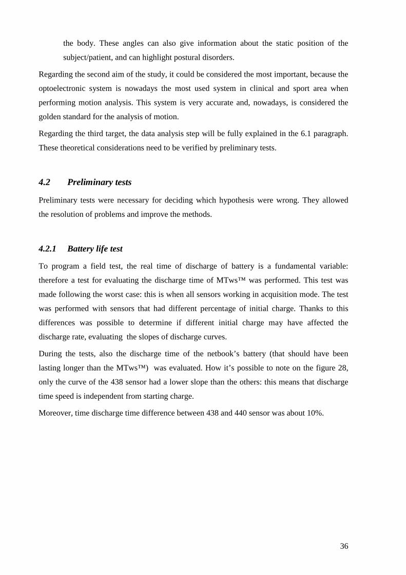
4.2.2 Magnetic field test
Another preliminary test for understanding the MTws™ features was performed with the
following aim: evaluating the influence of aluminium (paramagnetic material) on the Xsens’
magnetometer.
During this test, both the 442 and 436 sensors were placed on two aluminium bars, the
Alignment reset was performed to sensors 442, whereas no reset was performed on sensor
442. This different approach can show possible differences of electromagnetic interaction of
the sensor to which the reset was performed with respect to the other sensor.
Initially both sensors need a short time to stabilize themselves. At the end of this transient
period, it has been possible to appreciate a low interference due to aluminium and a good
stability of the sensors. You may notice in the chart below that the Z axis was the less stable
and that the sensor 442 (with the Alignment Reset) has given in output values between -4.6°
and -0.5°, while for sensor 440 (without reset), the values range is between -69.04° and -
72.36°.
38
Fig 29:Sensor 442 angles
Fig 30: Sensor 436 angles
39
This test highlighted limited and a comparable variations of the angles, possibly due to the
aluminium bar nearby. However only the Yaw angles had variations higher than 1°, and they
are limited to about 4°; therefore the aluminium hasn't a strong influence on the MTws™.
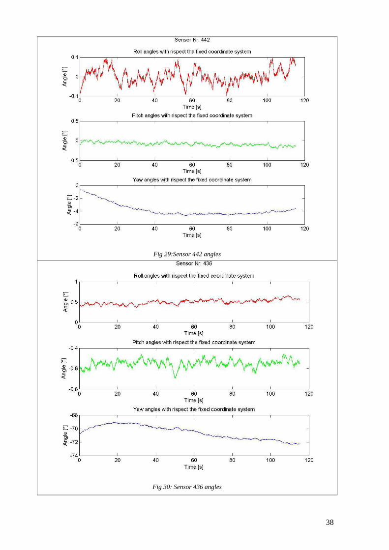
4.2.3 Pilot ski tests at the Cermis ski area
The first field test was planned to study several cross country skiing techniques. The test was
performed the 4th of April at the Alpe Cermis (TN), using 5 MTws™ produced by Xsens
Technologies. Snow was very soft due to a subtle rain in the second part of the morning, with
a temperature about 8°C.
The subjects were three cross country professionals, two men and one woman:
Subject Sex Weight Height Status Z.C. Man 184 [cm] 78 [Kg] Active
V.A. Man 181 [cm] 80 [Kg] Active B.E. Woman 158 [cm] 52 [Kg] Not Active
The test was divided in two parts: the first part was a snowplough braking technique test, the
second was a cross-country skiing technique test (with a basic calibration of body segments).
First of all, the biggest problem to solve, was to avoid wetting the Xsens sensors, and, at the
same time, fixing the sensors to the ski with the best stability. It was decided to fix two
sensors to the ski, because the researched data during this test where the angles formed by the
skier (respect the parallel ski position) during the snowplough braking technique and the
acceleration corresponding. Xsens was coated with a transparent film, for a basic, waterproof
pack. To avoid possible hole or infiltrations through this thin material, both Xsens were
covered with duct tape. So a small, but strong, waterproof package was obtained.
Fig 31: Xsens position on the ski

40
As reference point the boot binding was taken. Doing this all sensors were placed in the same
position for all subjects, independently from the different equipment and the subject's body
characteristics. The Xsens were fixed with the duct tape in the anterior part (from boot tip to
ski tip) of ski: the first sensor (cod. 438) at a distance of 175 mm and the second one (cod.
442) at 240 mm from the binding. These positions were safe for the sensors and were
characterized by high stability on the ski; the distance, as you can see in the picture, “was
forced” due to boot binding size.
Two different types of measurement system setup were defined:
Measurement System Setup 1
Sensors Sensors position Orientation
reset Fs [Hz]
438 17,5cm of boot binding
(X>0 Xsens system frame)
Alignment reset
120
442 24 cm of boot binding (X>0 Xsens system
frame)
Alignment reset
120
Measurement System Setup 2
Sensors Sensors position Orientation
reset Fs [Hz]
438 The same of MSS 1 Alignment
reset 120
442 The same of MSS 1 No reset 120
• The Alignment Reset was performed when skier was in the start position, with
parallels skis. This allows to obtain directly the angle between skis' reset position and
skis' position during snowplough braking;
• No reset means Xsens data will be output respect the Earth system of reference.
The presence of two sensors allowed to obtain the data regarding the angles from 438 sensor
and the acceleration/angular velocities from sensor 442. Lastly, to complete subject's
equipment, the netbook and the Awinda Station were placed in a small backpack, worn by
each subject during the test. The Awinda station in the backpack was always close to the
sensors, with a lower possibility of loss of signal and data.

41
Fig 32: Subject with equipment Fig 33: Detail of Xsens on the ski
Snowplough braking technique tests were performed like this:
1. The subject stood with parallel skis, in the start position;
2. Alignment reset was performed, according to the MSS type;
3. The recording was started with the MT manager software and the PC was inserted into
the backpack;
4. The subject began the descent pushing along the first 10/15 metres, then he continued
with parallel skis, finally he concluded with snowplough braking technique;
5. The recording was stopped with subject stood in the snowplough brake position.
This test was performed for both left and right ski for every subject, with different
measurement system setup, like synthesizes the following table:
Test Nr. Subject Starting time MSS Sensor position
0 Z.C 10:35 1 Right ski 1 Z.C 10:39 1 Right ski 2 Z.C 10:40 1 Right ski 3 Z.C 10:42 1 Right ski 4 Z.C 10:54 2 Left ski 5 Z.C 10:56 2 Left ski 6 Z.C 10:58 2 Left ski 7 V.A. 11:02 2 Left ski 8 V.A. 11:04 2 Left ski 9 V.A. 11:06 2 Left ski 10 V.A. 11:09 2 Right ski 11 V.A. 11:10 2 Right ski 12 V.A. 11:12 2 Right ski 13 B.E. 11:27 2 Right ski 14 B.E. 11:29 2 Right ski 15 B.E. 11:31 2 Right ski 16 B.E. 11:34 2 Left ski 17 B.E. 11:36 2 Left ski 18 B.E. 11:38 2 Left ski

42
Fig 34: Alignment Reset and start recording
Fig 35: 10/15 m of parallels ski descent
Fig 36: Snowplough braking step
Fig 37: Stop recording
The second part of the test was formed by two operations:
1. Calibrations of subjects’ body segments
2. Acquisition of cross-country skiing technique
These two topics can be exposed separately without modifying the linear development of this
work, indeed the calibrations of subjects’ body segments can be interpreted as a successive
step: so, for continuity and clarity of exposition, it will be explained in the chapter 6.
In this paragraph the procedure adopted for performed this test will be explained.
The first subject (Z.C.) was equipped with five sensors following the Measurement System
Setup schematize in this table
Measurement System Setup 3
Sensors Sensors position Fs [Hz]
438 Ski → 17,5 cm 75
442 Boot 75
436 Shank 75
439 Thigh 75
440 Sacrum 75
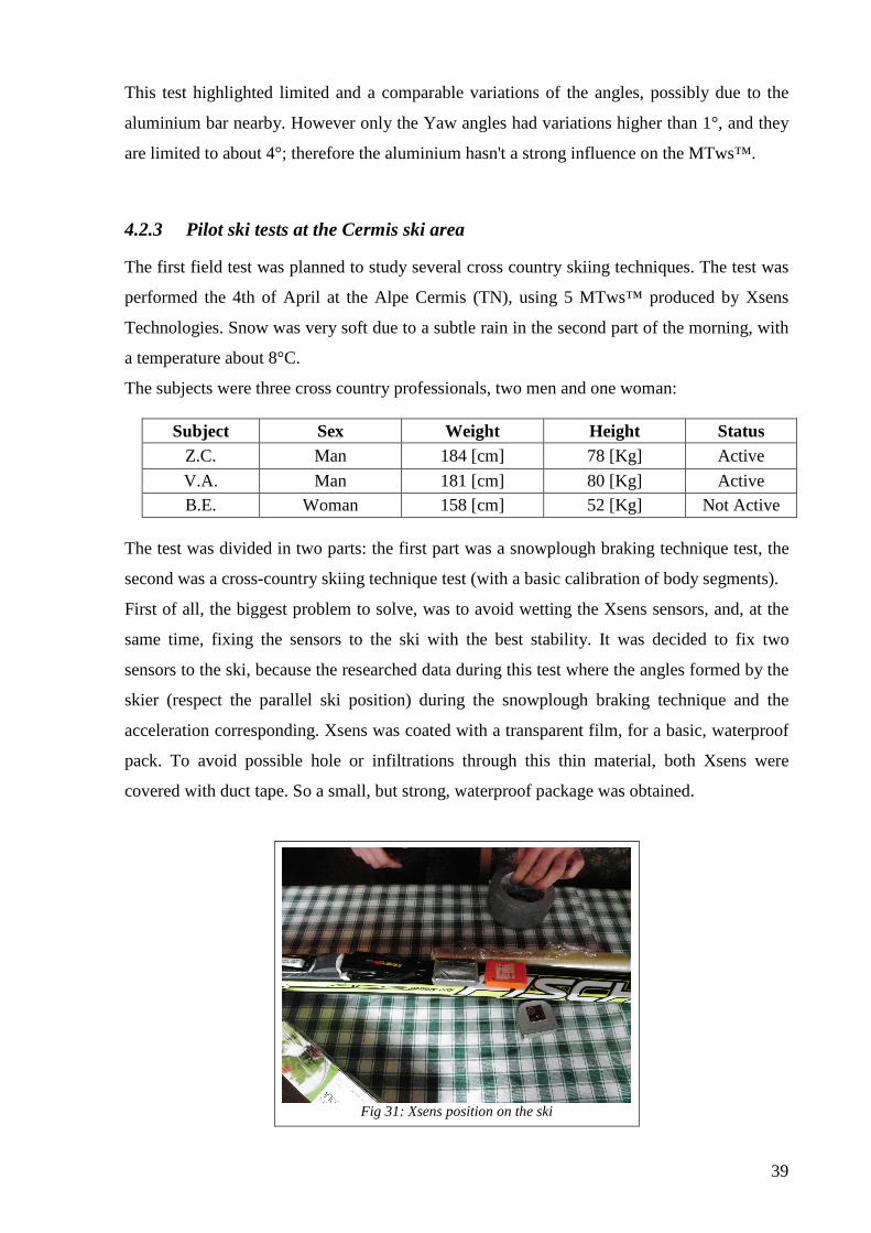
43
Fig 38: Sensor on the ski
Fig 39: Sensor on the boot
Fig 40:Sensor placed on subject
Each test was repeated in two Xsens configurations:
1. No reset 2. Alignment reset made on static standing
After this tests, the subject was invited to perform various skate skiing techniques in a short
stretch of track, a "U" trajectory was followed, with a gentle downhill in the first part,
followed by a 180 degrees rotation and finally the same length of track with, obviously, a
gentle uphill.
Sensor 442
Sensor 440
Sensor 439
Sensor 436
Sensor 438
44
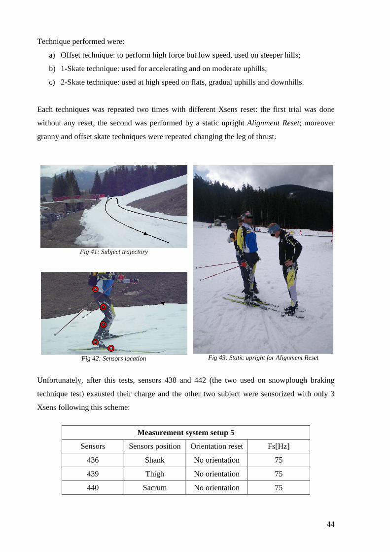
Technique performed were:
a) Offset technique: to perform high force but low speed, used on steeper hills;
b) 1-Skate technique: used for accelerating and on moderate uphills;
c) 2-Skate technique: used at high speed on flats, gradual uphills and downhills.
Each techniques was repeated two times with different Xsens reset: the first trial was done
without any reset, the second was performed by a static upright Alignment Reset; moreover
granny and offset skate techniques were repeated changing the leg of thrust.
Fig 41: Subject trajectory
Fig 42: Sensors location
Fig 43: Static upright for Alignment Reset
Unfortunately, after this tests, sensors 438 and 442 (the two used on snowplough braking
technique test) exausted their charge and the other two subject were sensorized with only 3
Xsens following this scheme:
Measurement system setup 5
Sensors Sensors position Orientation reset Fs[Hz]
436 Shank No orientation 75
439 Thigh No orientation 75
440 Sacrum No orientation 75

45
The subject performed classic skiing technique on the same track of the first subject, roughly
along the same trajectory. In the first time no reset was done to Xsens subsequently the
Alignment Reset in the physiological standing position was performed.
The third subject executed the same tests as the second subject: for the last test, another type
of Xsens reset was explored: when Alignment Reset is performed with wearing sensors, real
posture of person is lost because this operation set a new coordinate frame for each sensors;
for these reasons the Alignment Reset Pack was introduced.
The primary aims of the tests were: to assess the difference among three reset procedures, to
understand which of these is more recommended for biomechanical applications, and to have
a feedback regarding the MTws’ behaviour when performing sports acts in several operative
conditions. Considering the amount of data obtained during the tests, and the corresponding
lengthy and complicated analysis, we will be report directly the results for brevity.
In subjects opinions the sensors did not interfere with motions, the straps were sufficiently
fixed to avoid slippage, and, at the same time, did not limited the muscular normal activation.
The information about the physiological reference position are valuable data because they
allow to know the initial subject/patient position (including the Xsens positioning error). For
this reasons, because the Object and Heading Reset do not set all angles to zero, these two
type of reset were classified not adapt for this applications. The same consideration can be
done when the Earth coordinate system is taken as reference, and if the Alignment Reset is
performed with the subject standing in the physiological reference position. In this last case,
the first angles value returned are all zero and they don’t give information about the
subject/patient physiology or about MTws™ positioning but only about the relative motion
of the segments from the physiological reference position. Considering this reset features, the
Alignment reset pack should be the best for biomechanical applications, because it can give
both technical and anatomical information having set the same coordinate system for all
sensors.
4.2.4 Reset and angular velocity test
This paragraph will be recalled in chapter 6, where we will analyze the subjects’ body
calibration target: however this test was performed due to an incongruence highlighted during
the previous pilot ski tests. This can be also classified as a preliminary test because it allowed
understanding more features of MTws™. During data analysis of Cermis some
inconsistencies were detected between the orientation data and the angular velocity data: the
in fact latter were output with respect to axes differing from those used for the orientation
46
data: therefore other tests were planned in laboratory in order to understand the reasons of
these unexpected results. Aim of the tests was to clarity the different axes used for the
orientation data and the angular velocity data.
The first step of these tests consisted in simple movements around fixed axes, with the 436
MTw™ fixed on a totally non-ferromagnetic support. An Alignment Reset allowed to redefine
the system coordinate frame and, after a validation of reset, three simple rotation around the
coordinate system axes of the new coordinate system S’ were performed.
Results suggested that the orientation data are calculated with respect to the reset coordinate
frames’, but there wasn't correspondence with the angular velocity data.
The second step of the test was carried out with two Xsens (440 and 439), both sensors were
fixed at the same non-ferromagnetic support, performing the some movements. To the sensor
440 sensor the Alignment Reset was imposed to redefine its coordinate frame in this way:
o New Z' axis coincident with Z axis of sensor coordinate system S;
o New X' axis opposite with Y axis of S;
o New Y' axis coincident with X axis of S.
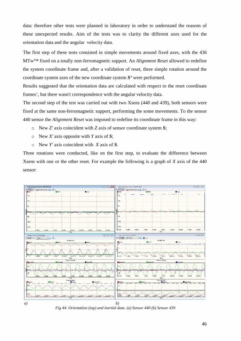
Three rotations were conducted, like on the first step, to evaluate the difference between
Xsens with one or the other reset. For example the following is a graph of X axis of the 440
sensor:
a) b) Fig 44: Orientation (top) and inertial data. (a) Sensor 440 (b) Sensor 439
47
In this graph is possible to note that when the 439 sensor is moved about Y axis, the angular
velocity data are correctly returned about Y axis (Pitch angles). Regarding the 440 sensor, the
motions were related to the X’ due to the Alignment Reset, but the angular velocity data are
still related to the Y axis. Moreover, even it the X’ axis was opposite to Y axis, the orientation
follows a correct trend but the angular velocity data are the same of both sensors.
Other tests reported the same results with an Object Reset. The conclusion taken is as follows:
the orientation data and the angular velocity data are related to the same coordinate frame
once that the reset is performed. More precisely the orientation data are calculated with
respect to the new coordinate frame S’ for the sensor 440, to which an Alignment Reset was
performed. However the angular velocity data are calculated with respect to the sensor
coordinate frame S.
This evidence is not corresponding to the Xsens User Manual, that reports “Once this
Alignment Reset is conducted, both inertial (and magnetic) and orientation data will be output
with respect to the new S' coordinate frame.” [Pg. 54 for Object Reset and 55 for Alignment
Reset].
However the angular velocity is defined as the rate of change of angular displacement and it is
calculated like the first derivative of the angular values, so, if angular velocity data were
calculated with respect to the new coordinate system S’, and the orientation data about the Y’
axis of the 440 sensor are nulls or constant, the angular velocity data about Y’ axis should be
null.
To bypass this incongruence, the angular velocity data are calculated by derivation from the
orientation data in the Matlab software created to analyze data. This solution will be explained
in details in Chapter 7.
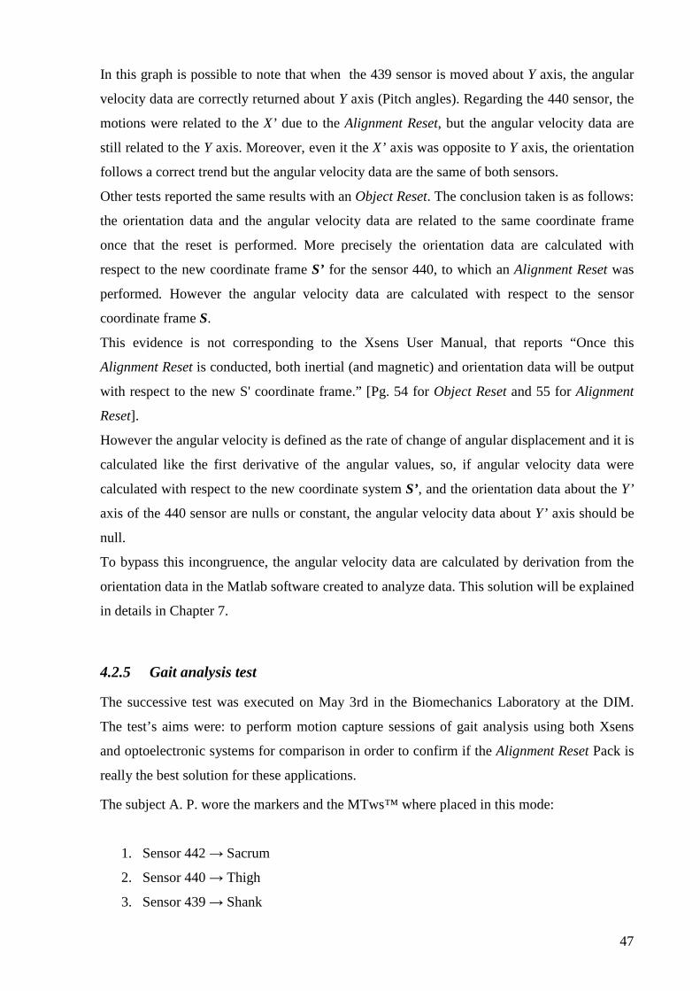
4.2.5 Gait analysis test
The successive test was executed on May 3rd in the Biomechanics Laboratory at the DIM.
The test’s aims were: to perform motion capture sessions of gait analysis using both Xsens
and optoelectronic systems for comparison in order to confirm if the Alignment Reset Pack is
really the best solution for these applications.
The subject A. P. wore the markers and the MTws™ where placed in this mode:
1. Sensor 442 → Sacrum
2. Sensor 440 → Thigh
3. Sensor 439 → Shank

48
4. Sensor 438 → Right foot
5. Sensor 436 → Left foot
To obtain comparable results from both systems, it was fundamental that each marker forming
the frame and the correspondent MTw™ would to the same movements. This consideration
can be obtained with the three markers (needed for creating a reference frame) placed as
closer as possible to the correspondent MTw™, and with a perfect coupling in order to
transmit the same motion to both systems. It is evident that this solution is impossible,
because markers must have a minimum distance between each other to be distinguished by
the optoelectronic system. All of these reasons led to this solution: the body strip has a plastic
clip to contain the MTw™ and under it there is a small slot. Two small aluminium supports
with a “T” shape were created , the longer segment was inserted under the strip’s plastic clip
and, on the three ends, were placed the three markers (Figure 44).
Fig 45: Embedded system obtained
By this way an embedded system was obtained and both MTw™ and optoelectronic systems
recorded the same motions. Measures however aren’t error-free because it can be a different
alignment between MTw™ axes and axes reconstructed from markers, moreover Xsens
Technologies said that it can be an error about 3° between real MTw™ position and its
external box.
During this test, the two “T” structures were positioned under the strap of the sensors attached
to the Thigh and the Shank. Moreover T shaped structures were covered by a dark tape to
avoid reflects that could be revealed by video cameras. The three markers on the aluminium

49
structure formed a so called “technical frame”, because it doesn’t gives directly anatomical
data.
The Alignment Reset Pack was modified because, if sensors have the X axis pointing upwards
during the operation of reset, when the Alignment Reset is performed, the system can’t
uniquely identify direction and orientation of the new X’ axis. Therefore, to decide direction
and orientation of X axis, the pack of MTws™ must have an inclination which identify the
direction that the new X' axis should take. To simplify the reset operation, a totally non-
ferromagnetic horizontal surface was prepared on which the MTws™ were positioned during
the reset. Using this device the reset pack is simpler and, it performed on an horizontal surface
with orthogonal faces, allows to obtain the same coordinate system for all sensors. Moreover
to choose the desired direction of new X’ axis is sufficient to tilt the surface and to measure
the angle formed with an inclinometer, called Reset angle. Knowing the Reset angle it is
possible to take into account during the data analysis step, obtaining results which refer to the
coordinate system that would be created performing the Alignment Reset Pack on a horizontal
surface. Summarizing, the Alignment Reset Pack is performed on a horizontal surface tilted
(in the direction chosen for the new X’ axis) of a known Reset angle thanks to the
inclinometer. The Reset angle will be offset during the data analysis step, erasing totally the
effect due to surface tilt. The Reset angle of this test was -5.7° about the Y’ axis.
In this test, the new sensor coordinate system S’ imposed by the Alignment Reset Pack was:
• X’ axis on gait direction as ab-adduction axis;
• Z’ axis pointing upwards as intra-extra rotation axis;
• Y’ following the right hand rule as flex-extension axis.
•
The BTS optoelectronic system has set the default coordinate system:
• X axis on gait direction as ab-adduction axis;
• Y axis pointing upwards as intra-extra rotation axis;
• Z axis following the right hand rule as flex-extension axis.
In this test, worthwhile underline that Xsens and BTS hadn’t the same reference coordinate
system: the Xsens had the Y’ axis as flex-extension axis instead the BTS system used the Z
axis. The results in this chapter are exposed to present the difference obtained between the
two system with these coordinate systems. The new method (exposed on Chapter 5) are
developed to fix the discordance obtained in these tests.

50
Fig 46: Sensor location
Fig 47: BTS coordinate systems
Fig 48: Xsens coordinate systems
However to compare the two systems, during the data analysis, the BTS coordinate system
was modified to obtain the same reference frame for both systems.
The BTS optoelectronic system has been calibrated obtaining this calibration volume
dimensions:
On X axis direction 3.85 [m]
On Y axis direction 1.98 [m]
On Z axis direction 1.65 [m]
Standard deviation 0.308
Mean 0.351
The subject was then asked to take a standing position (considered as the physiological
reference position for gait analysis test) to record the Static angles. After this, the subject
walked inside the calibrated volume to record the motions. Xsens Segment angles were
compared to the BTS Segment Angles only for the sensors 439 and 440, the only two with the
“T” structure.
Initially, the subject was invited to take the physiological reference position and the Static
angles returned are:

51
Sensor 436
(Left foot)
Sensor 438
(Right foot)
Sensor 439
(Shank)
Sensor 440
(Thigh)
Sensor 442
(Sacrum)
Roll (Φ) [°] -8.5183 2.0316 1.9113 4.4413 -6.0252
Pitch (Θ) [°] 17.4454 19.7934 -8.4150 -8.5471 14.0497
Yaw (Ψ) [°] 8.6101 -23.4352 -4.1818 0.3331 -6.8127
The subject of this test was healthy with no orthopaedic functional limitations, therefore these
Static angles give information only about the placement of MTws™ to the subject’s body.
First set of analyzed data were the Segment Angle:
Fig 49: Sacrum movement(Segment angles) Fig 50:Left foot movement(Segment angles)
Fig 51: Right foot movement(Segment angles)
In the graph of the sensor 442 it can be
observe the pelvis movements during walk,
with ab-adduction and the flex-extension
components due to the torsion of the trunk
when a leg is carried forward. The graphs of
the sensors 436 and 438 represent the
movements of the right and left foot. In all of
this graphs, between 5.8 and 6 seconds, the
subject performed an inversion of direction
of 180° anticlockwise. This motion is very
visible on the Yaw angle.
The graph below shows the Segment angles comparison, calculated by the Cardan angle
resolution:

52
Fig 52: Shank Segment angles comparison
Fig 53: Thigh Segment angle comparison
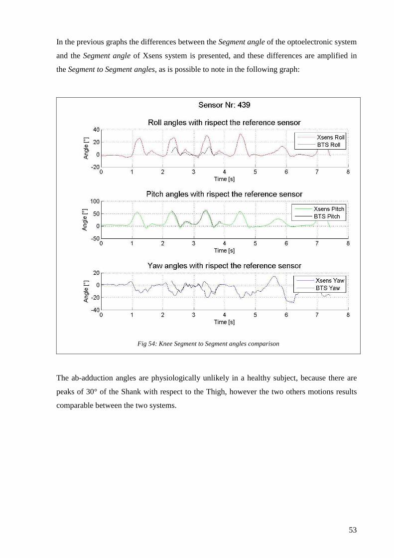
53
In the previous graphs the differences between the Segment angle of the optoelectronic system
and the Segment angle of Xsens system is presented, and these differences are amplified in
the Segment to Segment angles, as is possible to note in the following graph:
Fig 54: Knee Segment to Segment angles comparison
The ab-adduction angles are physiologically unlikely in a healthy subject, because there are
peaks of 30° of the Shank with respect to the Thigh, however the two others motions results
comparable between the two systems.

54
4.2.6 Treadmill test
After the gait analysis test, a treadmill test was performed with the same sensors and systems
configurations as the previous test. A treadmill with four markers at the extremity was
inserted in the calibration volume, and the subject was invited to run at two different speeds:
• 10 Km/h;
• 14 Km/h.
Fig 55: Subject during treadmill test
Following plots are presented side by side to compare the differences between the Segment
angles during the treadmill test at 10 km/h and the Segment angles at 14 km/h:5
5 Considering that the ab-adduction angles can’t be physiologically correct.
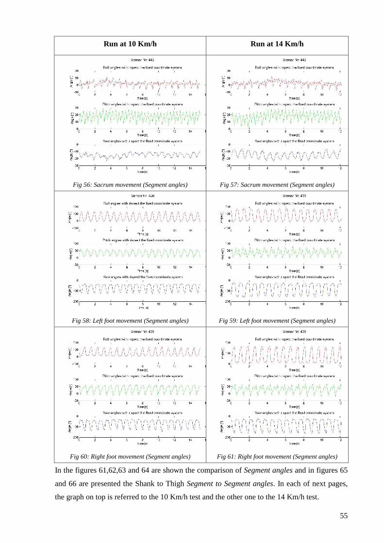
55
Run at 10 Km/h Run at 14 Km/h
Fig 56: Sacrum movement (Segment angles) Fig 57: Sacrum movement (Segment angles)
Fig 58: Left foot movement (Segment angles) Fig 59: Left foot movement (Segment angles)
Fig 60: Right foot movement (Segment angles) Fig 61: Right foot movement (Segment angles)
In the figures 61,62,63 and 64 are shown the comparison of Segment angles and in figures 65
and 66 are presented the Shank to Thigh Segment to Segment angles. In each of next pages,
the graph on top is referred to the 10 Km/h test and the other one to the 14 Km/h test.
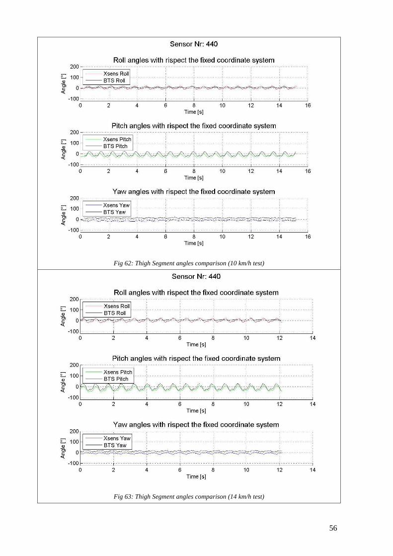
56
Fig 62: Thigh Segment angles comparison (10 km/h test)
Fig 63: Thigh Segment angles comparison (14 km/h test)
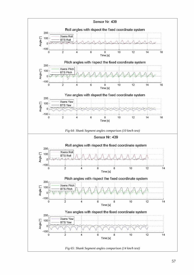
57
Fig 64: Shank Segment angles comparison (10 km/h test)
Fig 65: Shank Segment angles comparison (14 km/h test)
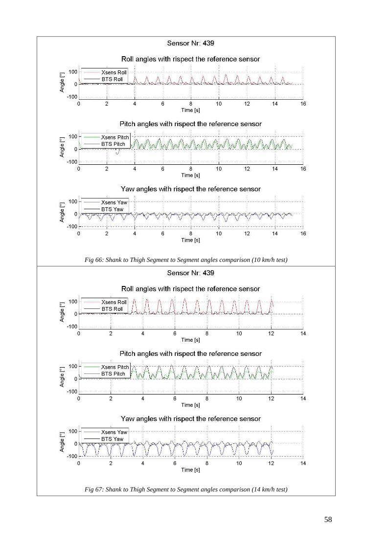
58
Fig 66: Shank to Thigh Segment to Segment angles comparison (10 km/h test)
Fig 67: Shank to Thigh Segment to Segment angles comparison (14 km/h test)

59
In this test the big differences between Xsens and optoelectronic system regarding the two
minor motion axes are evident, the axis with the larger movement are comparable. This test
also shows that the matching is of inverse proportionality than the motions speed, on the other
hand it is necessary to consider the higher possibility of artefacts, precisely due to motions
speed.
4.2.7 Starting blocks test
This test was carried out after the treadmill test: due to the previous tests, the video cameras
were moved and the BTS calibration was lost, so the optoelectronic data were not analyzed.
To perform this test, starting blocks were fixed to the force plate, into the calibrated volume
and a marker was dropped behind the subject as a start signal. By this way it was possible to
calculate the time between the moment in which the marker touched the floor and the moment
in which the subject started the motion. This is the reaction time of subject.
Fig 68: Starting block position Fig 69: Sensor placement
In the test analyzed, the subject had had a reaction time of 0.183 sec, however, for all test
made, the subject had always had a reaction time between 0.17 and 0.22 sec, which are typical
values of a healthy subject.
For the Segment angles, the most significant is the sensor 442, because recorded angles that
allow to reconstruct the position of subject on the starting blocks:
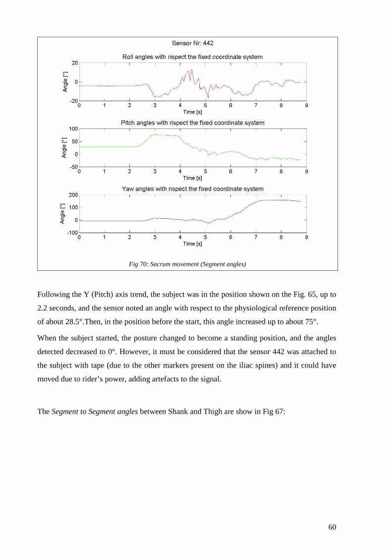
60
Fig 70: Sacrum movement (Segment angles)
Following the Y (Pitch) axis trend, the subject was in the position shown on the Fig. 65, up to
2.2 seconds, and the sensor noted an angle with respect to the physiological reference position
of about 28.5°.Then, in the position before the start, this angle increased up to about 75°.
When the subject started, the posture changed to become a standing position, and the angles
detected decreased to 0°. However, it must be considered that the sensor 442 was attached to
the subject with tape (due to the other markers present on the iliac spines) and it could have
moved due to rider’s power, adding artefacts to the signal.
The Segment to Segment angles between Shank and Thigh are show in Fig 67:
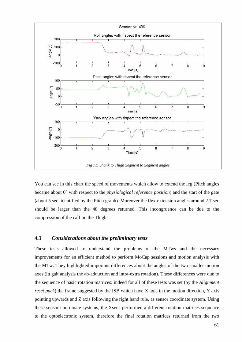
61
Fig 71: Shank to Thigh Segment to Segment angles
You can see in this chart the speed of movements which allow to extend the leg (Pitch angles
became about 0° with respect to the physiological reference position) and the start of the gate
(about 5 sec. identified by the Pitch graph). Moreover the flex-extension angles around 2.7 sec
should be larger than the 48 degrees returned. This incongruence can be due to the
compression of the calf on the Thigh.
4.3 Considerations about the preliminary tests
These tests allowed to understand the problems of the MTws and the necessary
improvements for an efficient method to perform MoCap sessions and motion analysis with
the MTw. They highlighted important differences about the angles of the two smaller motion
axes (in gait analysis the ab-adduction and intra-extra rotation). These differences were due to
the sequence of basic rotation matrices: indeed for all of these tests was set (by the Alignment
reset pack) the frame suggested by the ISB which have X axis in the motion direction, Y axis
pointing upwards and Z axis following the right hand rule, as sensor coordinate system. Using
these sensor coordinate systems, the Xsens performed a different rotation matrices sequence
to the optoelectronic system, therefore the final rotation matrices returned from the two

62
systems were not equal, and, inevitably, the angles calculated were not the same. The method
found to obtain the same angles between the two systems is explained in the following
chapter.
63
CHAPTER 5
Validation tests
5.1 Reset method
A final method for using the MTws™ reset is found. It is the Alignment Reset Pack, which is
performed with the horizontal device described in the previous chapter. The first step is to
identify the desired coordinate system and, after, MTws™ must be properly positioned for the
reset. To obtain the same new sensor coordinate system, the position on the subject’s body
where MTw™ should shall be evaluated. So, following how the Alignment Reset works, the
correct reset position for each MTw™ can be found.
As explained in the 4.2.5 paragraph, applying the reset in the horizontal tilted device, it is
possible to choose the direction of the X axis and, using an inclinometer, it’s possible to
measure the reset angle. Regarding the analysis data step, a particular “physiological rotation
sequence” is required: first, the axis around which larger movement is performed, second, the
axis around which intermediate movement is performed, third, the remaining axis. Every
MTw™ returns the Euler “aerospace” angles measured by a fixed rotation axis
XYZXYZ RRRR = (as explained in the 2.4 paragraph).
To perform the correct rotation sequence as defined “physiological rotation sequence”, there
are two possibilities:
1. Modify the rotation sequence;
2. Set the axes to perform the right sequence.
The first point can’t be applied because the Xsens executes a default X-Y-Z sequence, indeed
the output modes are: quaternion, Euler “aerospace” angles or rotation matrix terms.
The second approach can obtained by performing the Alignment Reset Pack as explained in
the previous chapter. If the reset is performed with the horizontal device tilted in the larger
motion’s direction, the X axis will have this direction and orientation, the Z axis will point
upward and the Y axis will be oriented according to the right hand rule.

64
Fig 72: Alignment Reset pack
This approach use the reset to set the sensor coordinate system, in the way that the Xsens
sequence rotation becomes equal to the “physiological sequence rotations”.
This method is fundamental for the comparison between Xsens and optoelectronic system and
its features will be explained in details in the successive paragraph.
5.2 Comparison between Xsens and optoelectronic system
The software of BTS optoelectronic system provides the users with multiple options for data
analysis, including the ability of creating the coordinate systems and the ability to rotate the
default laboratory reference system. When the reset is conducted following the method above
mentioned, Xsens and optoelectronic system further have different reference coordinate
system, but, using BTS software, it’s possible to change the BTS coordinate system to obtain
the same reference frame for both systems.
Once the same reference coordinate system and the same sensor/marker coordinate frame are
obtained for both systems, the Xsens return angles calculated according to the Euler
“aerospace” approach (XYZ sequence), whereas the BTS system return angles in according to
the Cardan representation. The different approach to calculate angles doesn’t affect the
determination of the final position of the coordinate system, because it must be the same, but
the intermediate rotations are different. Indeed the angles returned are different, because
Xsens performs rotations about fixed axes, whereas the BTS performs rotation around moving
axes. According to theory, when both systems refer to the same reference coordinate system
performing the same movements and the same sequence of rotations the resulting rotation
matrices must be equal. During the tests, the reference frame are modified to be the same for
both systems and the rotation must be:
� ( ) ( ) ( )ψθϕ '''''' zyXzXy RRRR = for the Cardan angles of the BTS system;
� ( ) ( ) ( )ΦΘΨ= XYzXYZ RRRR for the Euler “aerospace” angles of Xsens.
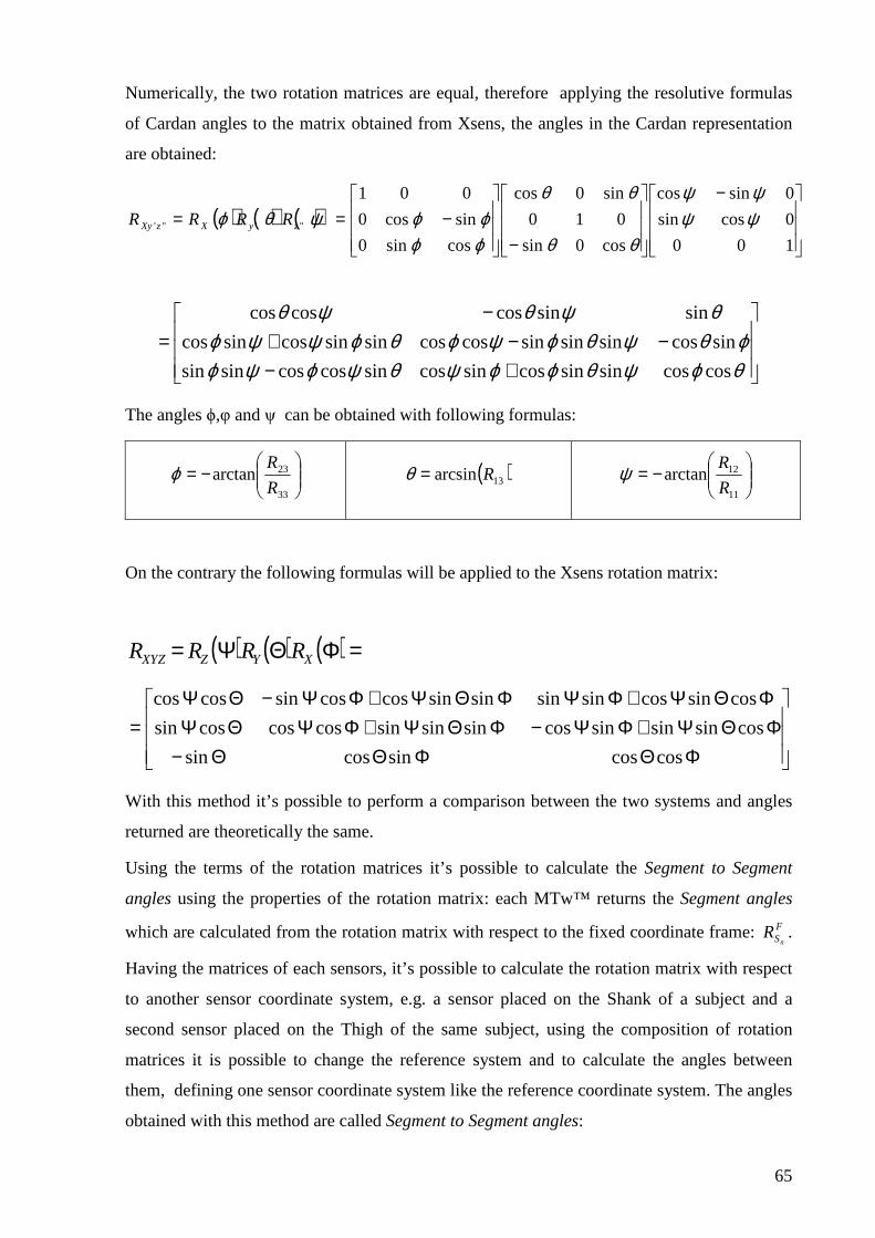
65
Numerically, the two rotation matrices are equal, therefore applying the resolutive formulas
of Cardan angles to the matrix obtained from Xsens, the angles in the Cardan representation
are obtained:
( ) ( ) ( )
−
−
−==100
0cossin
0sincos
cos0sin
010
sin0cos
cossin0
sincos0
001
'''''' ψψψψ
θθ
θθ
ϕϕϕϕψθϕ zyXzXy RRRR
+−−−+
−=
θϕψθϕϕψθψϕψϕϕθψθϕψϕθϕψψϕ
θψθψθ
coscossinsincossincossincoscossinsin
sincossinsinsincoscossinsincossincos
sinsincoscoscos
The angles ϕ,φ and ψ can be obtained with following formulas:
−=
33
23arctanR
Rϕ ( )13arcsinR=θ
−=
11
12arctanR
Rψ
On the contrary the following formulas will be applied to the Xsens rotation matrix:
( ) ( ) ( ) =ΦΘΨ= XYZXYZ RRRR
ΦΘΦΘΘ−ΦΘΨ+ΦΨ−ΦΘΨ+ΦΨΘΨ
ΦΘΨ+ΦΨΦΘΨ+ΦΨ−ΘΨ=
coscossincossin
cossinsinsincossinsinsincoscoscossin
cossincossinsinsinsincoscossincoscos
With this method it’s possible to perform a comparison between the two systems and angles
returned are theoretically the same.
Using the terms of the rotation matrices it’s possible to calculate the Segment to Segment
angles using the properties of the rotation matrix: each MTw™ returns the Segment angles
which are calculated from the rotation matrix with respect to the fixed coordinate frame: FSn
R .
Having the matrices of each sensors, it’s possible to calculate the rotation matrix with respect
to another sensor coordinate system, e.g. a sensor placed on the Shank of a subject and a
second sensor placed on the Thigh of the same subject, using the composition of rotation
matrices it is possible to change the reference system and to calculate the angles between
them, defining one sensor coordinate system like the reference coordinate system. The angles
obtained with this method are called Segment to Segment angles:
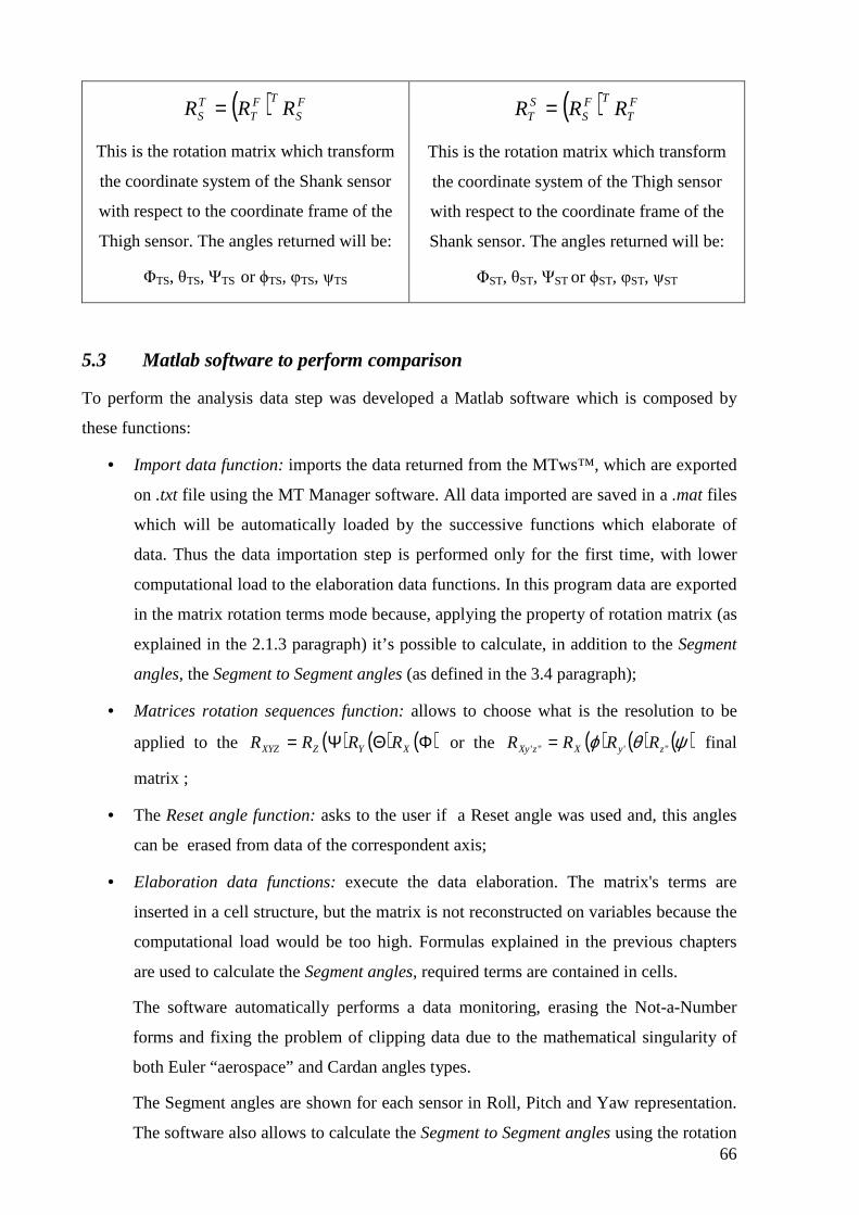
66
( ) FS
TFT
TS RRR =
This is the rotation matrix which transform
the coordinate system of the Shank sensor
with respect to the coordinate frame of the
Thigh sensor. The angles returned will be:
ΦTS, θTS, ΨTS or ϕTS, φTS, ψTS
( ) FT
TFS
ST RRR =
This is the rotation matrix which transform
the coordinate system of the Thigh sensor
with respect to the coordinate frame of the
Shank sensor. The angles returned will be:
ΦST, θST, ΨST or ϕST, φST, ψST
5.3 Matlab software to perform comparison
To perform the analysis data step was developed a Matlab software which is composed by
these functions:
• Import data function: imports the data returned from the MTws™, which are exported
on .txt file using the MT Manager software. All data imported are saved in a .mat files
which will be automatically loaded by the successive functions which elaborate of
data. Thus the data importation step is performed only for the first time, with lower
computational load to the elaboration data functions. In this program data are exported
in the matrix rotation terms mode because, applying the property of rotation matrix (as
explained in the 2.1.3 paragraph) it’s possible to calculate, in addition to the Segment
angles, the Segment to Segment angles (as defined in the 3.4 paragraph);
• Matrices rotation sequences function: allows to choose what is the resolution to be
applied to the ( ) ( ) ( )ΦΘΨ= XYZXYZ RRRR or the ( ) ( ) ( )ψθϕ '''''' zyXzXy RRRR = final
matrix ;
• The Reset angle function: asks to the user if a Reset angle was used and, this angles
can be erased from data of the correspondent axis;
• Elaboration data functions: execute the data elaboration. The matrix's terms are
inserted in a cell structure, but the matrix is not reconstructed on variables because the
computational load would be too high. Formulas explained in the previous chapters
are used to calculate the Segment angles, required terms are contained in cells.
The software automatically performs a data monitoring, erasing the Not-a-Number
forms and fixing the problem of clipping data due to the mathematical singularity of
both Euler “aerospace” and Cardan angles types.
The Segment angles are shown for each sensor in Roll, Pitch and Yaw representation.
The software also allows to calculate the Segment to Segment angles using the rotation

67
matrix property explained in the previous chapter. The first sensor inserted on the
import data function, is taken as the reference sensor and, even for these angles a data
monitoring is performed. For all sensors inserted (excluding the reference sensor) the
Segment to Segment angles are calculated;
• Physiological reference position function: allows to calculate the Static angles and the
user can decide whether to delete these angles for the subsequent processing;
• Gait analysis comparison function: executes the comparison between Segment angles
or/and Segment to Segment angles given from BTS optoelectronic system and Xsens
systems. In this function an algorithm that synchronizes data (because during the tests
there wasn’t a trigger signal to set the same time of start) it’s implemented. This
algorithm calculates the range of time in which the optoelectronic system has recorded
the gait and it finds the maximum value. Moreover it is calculated the maximum peak
of Xsens data in the same range of time of the optoelectronic and the graph is
synchronized on the maximum value of the larger motions axis. This algorithm
performs the comparison both for Segment angles and Segment to Segment angles;
• Graphs save function: creates a folder in the original data’s folder for every types of
angles calculated and, in it, the software automatically saves all sensors' angles graphs.
5.4 Validation tests
These tests were performed to validate the method previously exposed and to perform
comparison between BTS optoelectronic system and Xsens system.
5.4.1 Electrogoniometer test
In this test an electrogoniometer was used only as structure to execute the test. This device
was chosen because it’s formed by two stems joined by a pivot, so it allows only one degree
of freedom. To place the sensors, it was traced the medial axis of each stems and both Xsens
and markers was placed in these positions:
1. “Fixed” marker on the joint
2. “Moving” marker on the superior stem’s
medial axis
3. “Tip fixed” marker on the inferior
stem’s medial axis
1. Xsens 440 on the superior stem’s medial
axis
2. Xsens 442 on the inferior stem’s medial
axis
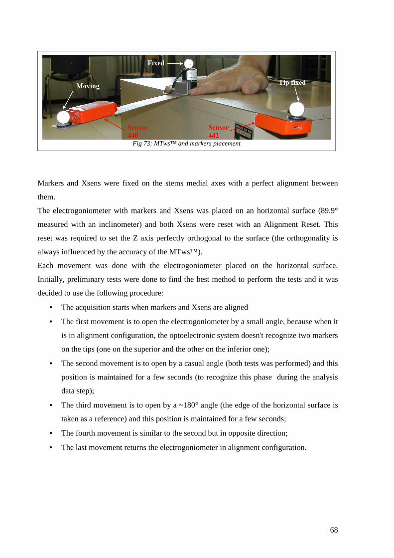
68
Fig 73: MTws™ and markers placement
Markers and Xsens were fixed on the stems medial axes with a perfect alignment between
them.
The electrogoniometer with markers and Xsens was placed on an horizontal surface (89.9°
measured with an inclinometer) and both Xsens were reset with an Alignment Reset. This
reset was required to set the Z axis perfectly orthogonal to the surface (the orthogonality is
always influenced by the accuracy of the MTws™).
Each movement was done with the electrogoniometer placed on the horizontal surface.
Initially, preliminary tests were done to find the best method to perform the tests and it was
decided to use the following procedure:
• The acquisition starts when markers and Xsens are aligned
• The first movement is to open the electrogoniometer by a small angle, because when it
is in alignment configuration, the optoelectronic system doesn't recognize two markers
on the tips (one on the superior and the other on the inferior one);
• The second movement is to open by a casual angle (both tests was performed) and this
position is maintained for a few seconds (to recognize this phase during the analysis
data step);
• The third movement is to open by a ~180° angle (the edge of the horizontal surface is
taken as a reference) and this position is maintained for a few seconds;
• The fourth movement is similar to the second but in opposite direction;
• The last movement returns the electrogoniometer in alignment configuration.

69
Fig 74: Example of a motion
The graph below represents the angles obtained during this test:
Fig 75: Segment angle of the electrogoniometer test
The angles are absolutely comparable to each other, however, in this test, the angles returned
from optoelectronic system are always larger than the Xsens angles. Differences recognized
are:

70
A1 A2 A3
3.25° 3.46° 3.8°
This test was repeated with comparable results, therefore an angle included between |3° ÷ 4°|
could be taken as the error between the BTS optoelectronic system and the Xsens MTws™
system.
5.4.2 2nd gait analysis test
The gait analysis test was a further validation test performed and it was executed following
the method explained previously. The subject was dressed with 5 MTws™ arranged in the
following way:
• Sensor 436 on left Shank;
• Sensor 438 on right Shank;
• Sensor 439 on right Thigh;
• Sensor 440 on left Thigh;
• Sensor 442 on sacrum.
One of the two “T” structures was placed on the right leg to create the marker’s technical
frame (as presented in the 4.2.5 paragraph).
The optoelectronic calibration system had reported this volume features:
On X axis direction 2.97 [m]
On Y axis direction 2.09 [m]
On Z axis direction 4.40 [m]
Standard deviation 0.297
Mean 0.345
The Alignment Reset Pack was performed with 10° of Reset angle around the Y axis, and it
had set this coordinate system:
• X axis as the Flex-Extension axis;
• Y axis as the Ab-Adduction axis;
• Z axis as the Intra-Extra rotation axis.

71
Initially, the subject was invited to take the physiological reference position and the Static
angles returned are:
Sensor 436
(Left Shank)
Sensor 438
(Right Shank)
Sensor 439
(Right Thigh)
Sensor 440
(Left Thigh)
Sensor 442
(Sacrum)
Roll (Φ) [°] -4.3940 -5.7050 -5.7000 -7.1091 -5.7690
Pitch (Θ) [°] -6.7397 7.8326 7.3349 -9.6506 -1.5315
Yaw (Ψ) [°] -13.6629 6.5644 -3.9286 12.6196 7.6297
The subject of this test is healthy with no orthopaedic functional limitations, therefore these
Static angles give information only about the placement of MTws™ on the subject’s body.
The subject walked for 3 times in the calibrated volume while both systems were recording
the motions. The comparison between the two systems was performed only for the 438 and
439 sensors, because “T” structure with markers were placed only behind these sensors.
First data analyzed were the Segment Angle of the first gait test:
Fig 76: Sacrum movement (Segment angles) Fig 77:Left Thigh movement (Segment angles)

72
Fig 78: Left Shank movement (Segment angles)
The first graph represents sacrum’s movement during walk: the sensor 442 was placed too
high, indicatively to L4-level because in the subject’s iliac crests were placed markers. For
this reason the movements recorded were not as expected. Other two graph reported the
movements of the left Thigh and the left Shank. Below are inserted 438 and 439 sensors’
graphs with, in black, the BTS Segment angles, and the Segment to Segment angles are shown
on the figure 76:
Fig 79: Thigh Segment angles comparison

73
Fig 80: Right Shank Segment angles comparison
Fig 81: Shank to Thigh Segment to Segment angles comparison
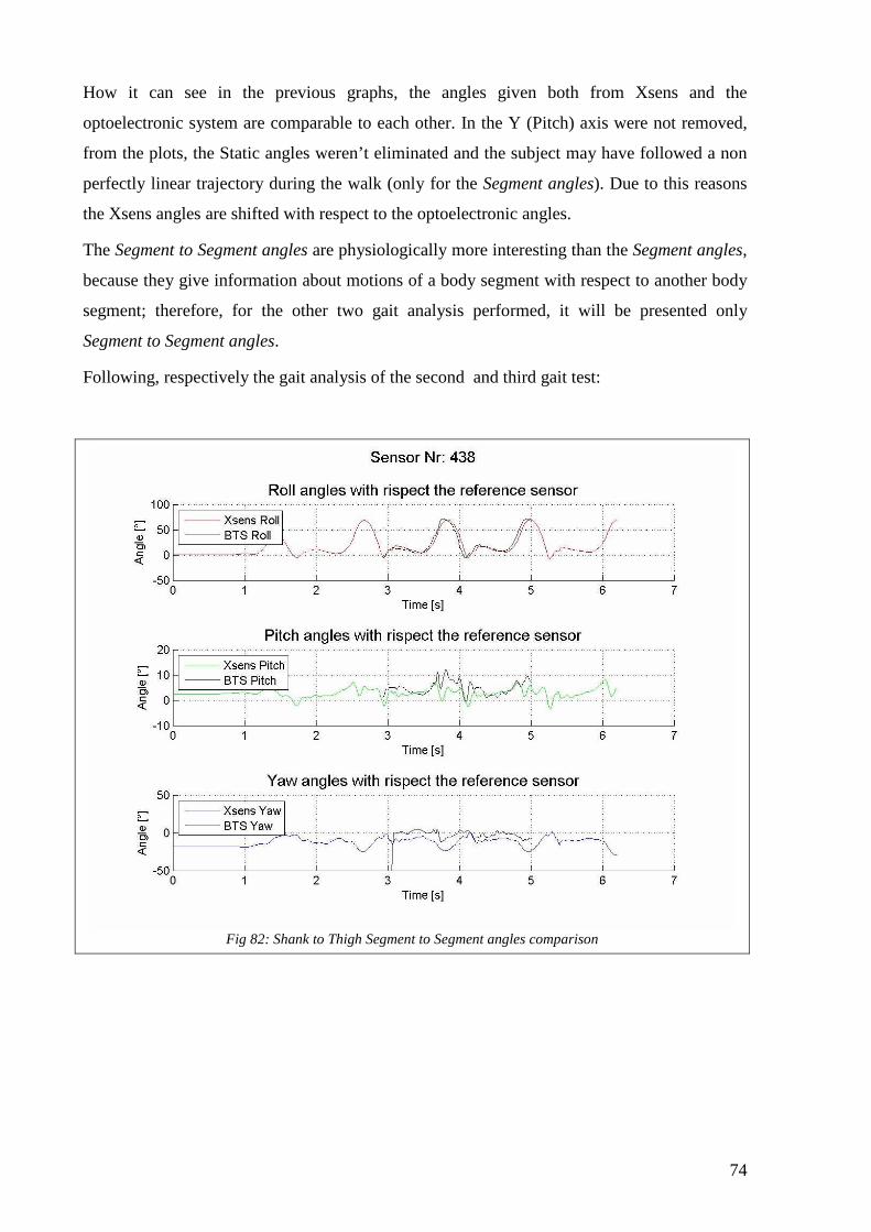
74
How it can see in the previous graphs, the angles given both from Xsens and the
optoelectronic system are comparable to each other. In the Y (Pitch) axis were not removed,
from the plots, the Static angles weren’t eliminated and the subject may have followed a non
perfectly linear trajectory during the walk (only for the Segment angles). Due to this reasons
the Xsens angles are shifted with respect to the optoelectronic angles.
The Segment to Segment angles are physiologically more interesting than the Segment angles,
because they give information about motions of a body segment with respect to another body
segment; therefore, for the other two gait analysis performed, it will be presented only
Segment to Segment angles.
Following, respectively the gait analysis of the second and third gait test:
Fig 82: Shank to Thigh Segment to Segment angles comparison

75
Fig 83: Shank to Thigh Segment to Segment angles comparison
As a conclusion, after analyzing the data in these graph, the optoelectronic flex-extension
angles result a generally about 10° larger than the corresponding Xsens angles. Regarding the
ab-adduction angles, they are generally more different from the others; however the
difference, considering graphs are shifted due to reasons explained in the first gait test of this
paragraph, is lower than 10°. Finally, intra-extra rotation angles are widely shifted, but in the
Segment to Segment angles it’s not considered the motion trajectory effect. This difference
could be given due to disturbance or magnetic fields, however, the angles amplitude is
comparable, with a difference lower than 10°.
5.4.3 Test of intensive care bed
MTws™ portability is one of the most important features of the Xsens, and it allowed to
perform a test session, in an intensive care room.
The test described in this chapter was executed at an intensive care room at the Padua’s
Hospital, to record the movements transmitted to a patient, when the intensive care bed, in
which he was lying, was mobilized by the hospital operators, the patient’s role was recited by
a volunteer workmate. Indeed, resulted some movements which not to be transmitted in the

76
correctly to the patient, first of all the motions in which the patient’s body is influenced from
the gravity force without the support needed, e.g. the trunk in sit position. Another problem is
the slip of the patient when a tilt movement is performed. Every movement which is not
correctly transmitted, may worsen the patient’s conditions. The test was performed with 5
MTws™ and 3 optical markers in order to evaluate both orientations and displacements of the
subject during bed's movements.
An Alignment reset pack with a tilt of 11.5° on the Y axis was performed on the 5 MTws™
and, this operation set the same sensor coordinate system to all sensors, formed by:
• X parallel to the sagittal plane;
• Z pointing upwards;
• Y following the right hand rule.
Subsequently the Xsens were placed on the subject following this scheme:
Sensor Position
436 Left Shank
438 Left Thigh
439 Sacrum
440 Left shoulder
442 Head (forehead)
Also the reflective markers were placed on three anatomical landmarks:
1. Left acromion;
2. Left greater trochanter;
3. Lateral epycondile of the left leg.
All the movements took take place in the XZ plane, because all motions were around the Y
axis, therefore to make simpler the data analysis, the Roll and Yaw angles can be considered
negligible with respect to the real motions performed around the Y axis.
Initially the subject was invited to stand in the physiological reference position and, to verify
the correctness of the reset, the subject also rested in horizontal position on the bed was taken
as a second physiological reference position. This means that for this test there are two
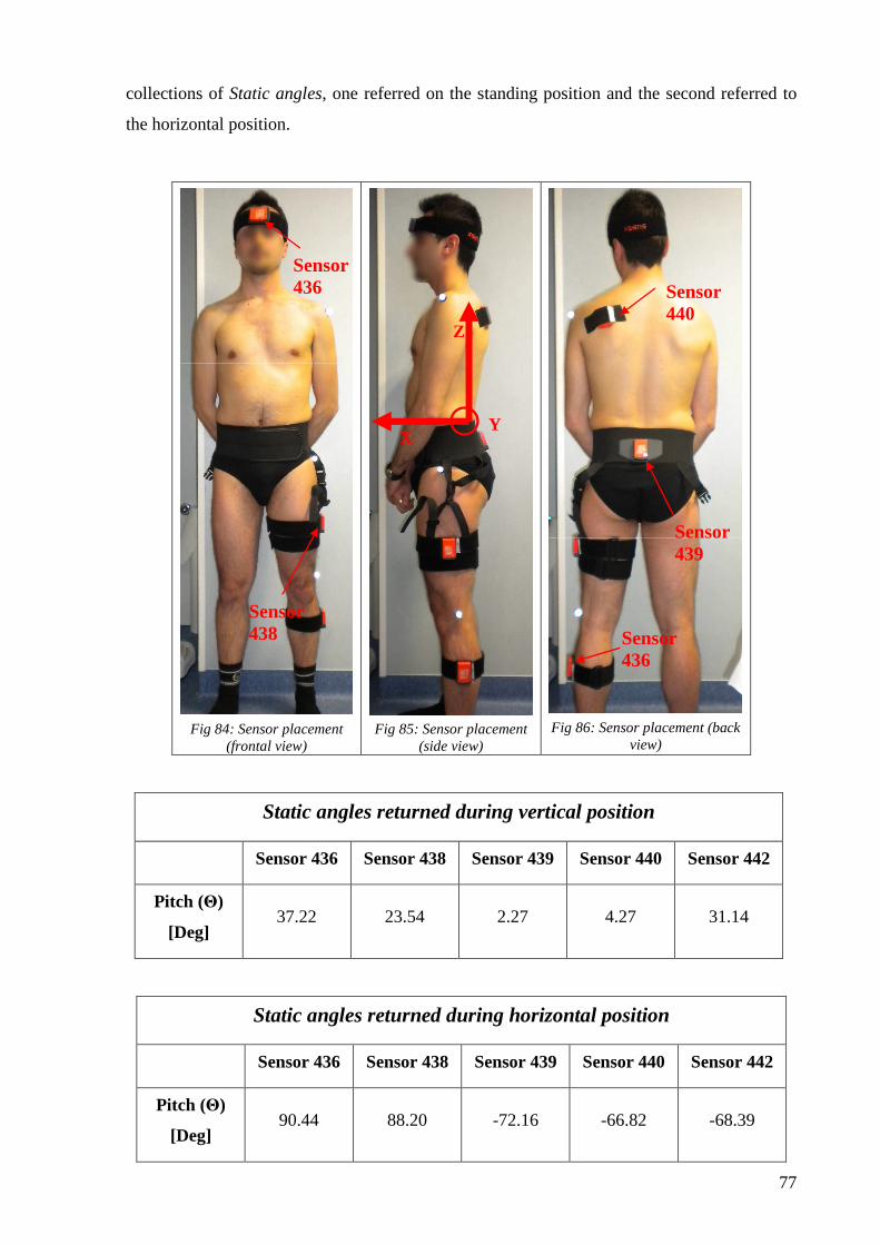
77
collections of Static angles, one referred on the standing position and the second referred to
the horizontal position.
Fig 84: Sensor placement (frontal view)
Fig 85: Sensor placement
(side view)
Fig 86: Sensor placement (back
view)
Static angles returned during vertical position
Sensor 436 Sensor 438 Sensor 439 Sensor 440 Sensor 442
Pitch (Θ)
[Deg] 37.22 23.54 2.27 4.27 31.14
Static angles returned during horizontal position
Sensor 436 Sensor 438 Sensor 439 Sensor 440 Sensor 442
Pitch (Θ)
[Deg] 90.44 88.20 -72.16 -66.82 -68.39
X
Z
Y
Sensor 439
Sensor 440
Sensor 436
Sensor 438
Sensor 436

78
These data shown immediately an incongruence because two of five sensors had returned a
positive Pitch angles. When the subject was in horizontal position on the bed, Y axis rotation
was about -90 degrees with respect to the vertical physiological reference position, if the Y
axis was in the expected direction. These discordances can be due only to problems resetting
being performed: later on it was found that in the bottom part of the bed there were two
permanent magnets. The magnetic fields produced by the magnets, may have been the cause
of these three sensors wrong reset. However, this inconvenience was fixed during the analysis
data step and the trend of the graph can be considered as more correct.
The most interesting movements done, were:
0° trunk
and
0° leg
30° trunk
and
0° leg
45° trunk
and
0° leg
30° trunk
and
0° leg
30° trunk
and
10° leg
0° trunk
and
0° leg
In the following table there is a summary of averages of Static angles returned from MTws™
which represent the subject movements in according to the intensive care bed movements:
442
(Head) 440
(Left shoulder) 439
(Sacrum) 438
(Left Thigh) 436
(Left Shank)
Trunk at 30°
-25,9 30,89 28,31 6,13 2,13
Trunk at 45°
-40,8 38,38 31,33 4,47 4,64
Trunk at 30° and leg
at 10° -31,9 23,46 18,73 2,88 6,74
Trunk and leg at 0°
-4,6 2,85 -3,7 -3,85 -3,47
In the next page are reported the graphs of angle values returned by MTws™ with a graphical
representation of the bed movements.

79
Sensor 442
Sensor 440
Sensor 439
Sensor 438
Sensor 436
Fig 87: Comparison between subject and bed movement

80
The values found show initially that movements transmitted to the subject are generally lower
than the bed’s movements. This result was expected, initially because the mattress can not
transmit the total bed’s movements to the subject, but, also because some parts of motion are
lost due to the subject’s movements on the bed, as slip effect. Moreover the data show a link
between trunk and leg movements, even if these movements were performed separately.
Test like this can allow to design intensive care beds more and more comfortable for the
patient, focusing attention on the patient and evaluating the real effect on patient of bed's
movements which, like shown in this test, are not perfectly coincident.
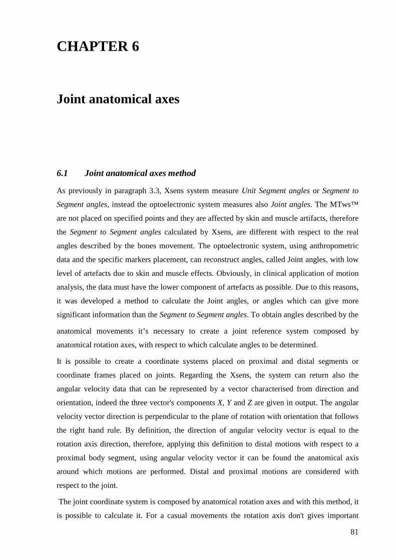
81
CHAPTER 6
Joint anatomical axes
6.1 Joint anatomical axes method
As previously in paragraph 3.3, Xsens system measure Unit Segment angles or Segment to
Segment angles, instead the optoelectronic system measures also Joint angles. The MTws™
are not placed on specified points and they are affected by skin and muscle artifacts, therefore
the Segment to Segment angles calculated by Xsens, are different with respect to the real
angles described by the bones movement. The optoelectronic system, using anthropometric
data and the specific markers placement, can reconstruct angles, called Joint angles, with low
level of artefacts due to skin and muscle effects. Obviously, in clinical application of motion
analysis, the data must have the lower component of artefacts as possible. Due to this reasons,
it was developed a method to calculate the Joint angles, or angles which can give more
significant information than the Segment to Segment angles. To obtain angles described by the
anatomical movements it’s necessary to create a joint reference system composed by
anatomical rotation axes, with respect to which calculate angles to be determined.
It is possible to create a coordinate systems placed on proximal and distal segments or
coordinate frames placed on joints. Regarding the Xsens, the system can return also the
angular velocity data that can be represented by a vector characterised from direction and
orientation, indeed the three vector's components X, Y and Z are given in output. The angular
velocity vector direction is perpendicular to the plane of rotation with orientation that follows
the right hand rule. By definition, the direction of angular velocity vector is equal to the
rotation axis direction, therefore, applying this definition to distal motions with respect to a
proximal body segment, using angular velocity vector it can be found the anatomical axis
around which motions are performed. Distal and proximal motions are considered with
respect to the joint.
The joint coordinate system is composed by anatomical rotation axes and with this method, it
is possible to calculate it. For a casual movements the rotation axis don't gives important

82
biomechanical information, but if the subject performs uni-axial motions around the
physiological axes (e.g. flex-extension, intra-extra rotation etc.), the angular velocity vector’s
direction must be equal to the corresponding anatomical axis direction of the motion
performed. To obtain the knee coordinate system following this method, necessary
independent motions are flex-extension, intra-extra rotation and ab-adduction. At this point, to
obtain significant data, movements must be as much more uni-axial as possible. Due to this
reason, two solution were adopted: creating a mechanical device which forced the movements
only around the axis to find or to define specific motions to perform in particular positions
minimizing unwanted movements. The use of mechanical device was discarded because it is
a more complex approach (and it could require a long time), but if the precision required are
very high, with such devices, the movements must be perfectly uni-axial. In the other hand
this approach would force the subject’s motions and eventually disorders wouldn’t be
identified.
The second solution, based on physiological, will be explained in the following paragraph.
6.1.1 Basic movements
The subject performed specific mono-axial movements, minimizing unwanted ones as
previously explained. Positions are defined according to the joint motions, e.g. to find the
knee coordinate system,designed positions are:
• Sit on a table to perform the flex-extension and the intra-extra motions;
• Standing position to perform the ab-adduction movements;6
Data acquired during tests were affected by artefacts due to thigh's muscles activation, so the
calculated subject’s joint rotation axes aren’t equals to anatomical ones. Due to this, calulated
axes are not quoted here.
The standing position is the designed position to find the hip coordinate system.
6 Precisely, the ab-adduction knee's motions should be performed with the subject in prone position, but this aim wasn’t improved, and the tests were mainly performed to verify the method

83
Fig 88: Calf intra-extra rotation Fig 89: Knee Flex-extension
Fig 90: Hip ab-adduction Fig 91: Hip flex-extension Fig 92:Hip intra-extra rot.
Basic movements defined upward are necessary to create the joint coordinate system, and
they are defined according to the joint’s motions. Due to this reason they could change from
joint to joint.
6.2 Matlab software to calculate rotation axes
Even for this aim a Matlab software which allows to analyze data was created. Thanks to the
modularity of the software created for the comparison, some functions exposed before are still
used for this application and the angles returned are the input of the new functions which
calculate the rotation axis:
• Time resize function: allows to redefine the length of the signal, to perform analysis on
the selected motion. This function is fundamental for the correct operation of the

84
motion axis function and to obtain less data to compute, because for every sample is
defined an angular velocity vector;
• Angular velocity function: was inserted due to the incongruence between orientation
data and angular velocity data (explained in the 4.2.4 paragraph). In this function is
calculated (following the definition) the angular velocity data starting from the
Segment to Segment angles data. The algorithm which perform the derivative was
created with this scheme:
o The discrete derivative of the first (n=1) sample is calculated using the
definition (the first forward difference):
−+Φ−+Φ=Φfs
nnnn
)1()()1()1(
. 7
o For the data between second to second-last samples, the discrete derivative is
calculated with this resolution:
−+Φ−+Φ=+Φfs
nnnnn
)2()()2()1(
8
o The discrete derivative of the last (n=length(Φ)) sample is calculated using the
definition (the first forward difference):
−+−Φ−Φ=Φfs
nnnnn
)1()1()()(
. 9
This resolution allows to obtain the angular velocity data expressed in the right
coordinate system: the comparison with the angular velocity given in output from
Xsens has revealed slight differences, mainly due to the data filtering done by Xsens;
• Motion axis function: performs a comparison between the X, Y and Z components of
the angular velocity vectors and the highest one is selected. The comparison is
performed by calculating the average of absolute values of each component, and by
taking the axis of higher value of angular velocity as the rotation axis. This
assumption may be correct considering two parameters: performing the basic
movements, the angular velocity of the motion axis should be much higher than the
other two components and it is fundamental, using the time resize function, to erase
each signal's segment that doesn’t contain information about the motions ( e.g. initial
subject's positioning or other movements not required);
7,8,9 fs is the sampling frequency and the angle Φ is taken as example.

85
• Threshold function: applies a threshold, selected by the user, to the angular velocity
data. To increase the threshold effect it is applied to the vector’s module and the
values included between [+threshold ÷ -threshold] are erased. Indeed the low angular
velocity data, refers to slower motions mainly affected by errors. Lastly, the same
samples erased in the vector’s module are erased in the axis of higher motion,
recognized with the Motion axis function;
• Rotation axis function: calculates the rotation axis from the angular velocity vectors.
The rotation axis can be considered as the average of all angular velocity vectors of
the axis recognized with the Motion axis function. To find the average of these
vectors, the averages of X,Y and Z components of every vectors are calculated, and the
rotation axis, which is equal to the anatomical rotation axis, should be identified by the
three coordinates found. The anatomical rotation axis found is expressed in the
coordinate system of the sensor taken as reference. E.g. to calculate the flex-extension
rotation axis of the knee, the subject must be invited to perform the flex-extension
movements, trying to limit others motions, and the angular velocity vector must be
calculated from Shank to Thigh Segment to Segment angles, so that the direction of
the angular velocity vectors are coincident with the knee flex-extension axis.
6.3 Validation test
The electrogoniometer test can be used as validation test for the method used to find the
rotation axis: indeed for all test the electrogoniometer had performed movements around the Z
axis, because all motions were performed on the horizontal surface. Analyzing data steps are:
Fig 93: Angular velocity diagram

86
This graph show the angular velocity data returned from the angular velocity function. The
figure below highlight the correspondence between orientation and angular velocity data:
Fig 94: Correspondence between orientation and angular velocity data
To erase the small peak at 8.23 seconds, the Time resize function is used and the signal up to
10 seconds is cut. The graph below represent the angular velocity vectors:
Fig 95: Angular velocity vectors
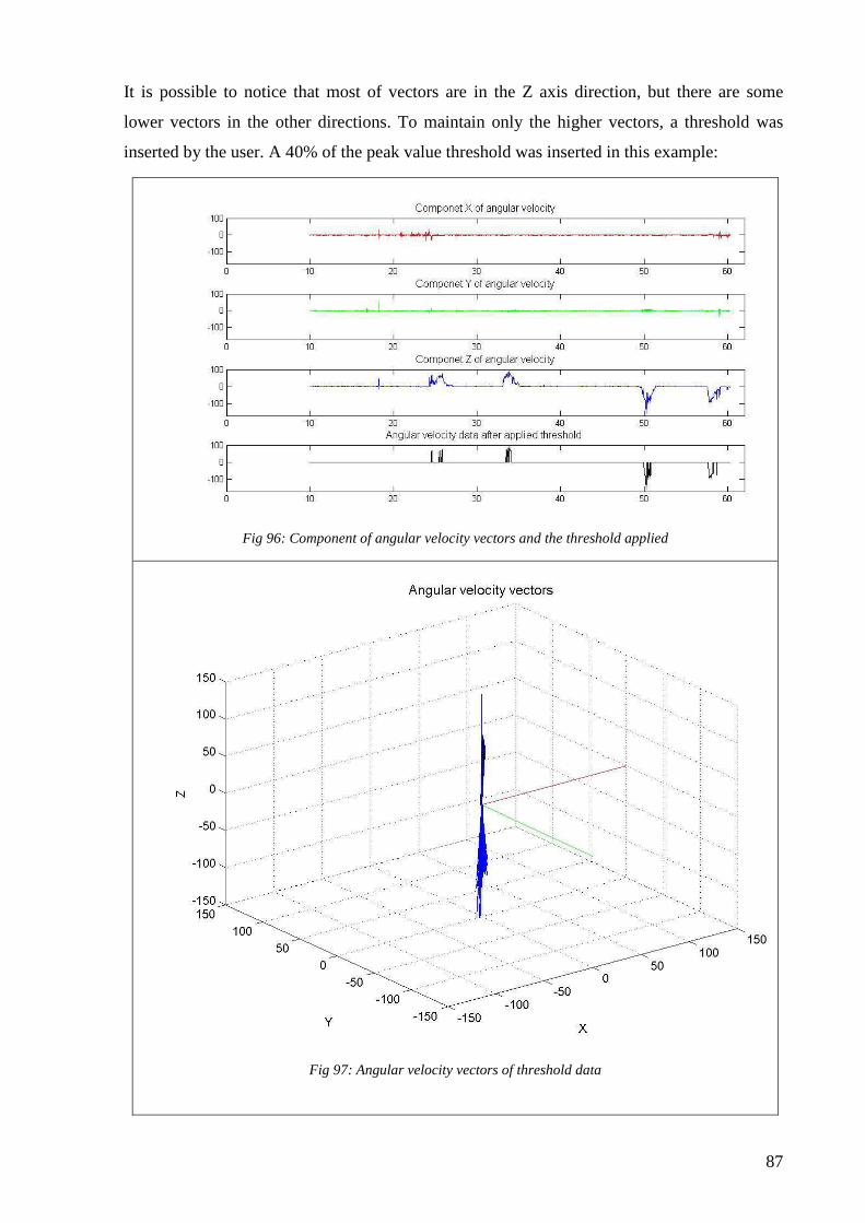
87
It is possible to notice that most of vectors are in the Z axis direction, but there are some
lower vectors in the other directions. To maintain only the higher vectors, a threshold was
inserted by the user. A 40% of the peak value threshold was inserted in this example:
Fig 96: Component of angular velocity vectors and the threshold applied
Fig 97: Angular velocity vectors of threshold data

88
All vectors lower than the threshold are erased, and, using the rotation axis function the
rotation axis is calculated:
Fig 98: Rotation axis founded (XZ plane view)
Fig 99: Rotation axis founded (YZ plane view)
The rotation axis calculated, as is can see in the previous graphs, is not perfectly coincident to
the Z axis, because the superior electrogoniometer’s stem was flexed due to the weight of the
MTw™ placed on the tip. Considering this error during the test, the rotation axis calculated
coincides with the one expected, therefore this test had confirmed the correctness of the
method used.

89
CHAPTER 7
Conclusion
7.1 Conclusions
Inertial sensors, like the Xsens MTw™ used for tests made, are having rapid diffusion in
several application areas, from biomechanics field to entertainment. Both portability and
easiness of use are the main features behind this rapid commercial expansion.
The methodologies developed during this work, based on a particular reset approach and a
specific angles sequence resolution, allows to perform comparison between Xsens MTw™
product and BTS optoelectronic system.
The analysis of test demonstrates that the two systems have a comparable accuracy, with a
difference of about 3 degrees calculated during a uni-axial test. Regarding 3D tests, as gait
analysis, the Flex-Extension’s graph generally can be superimposed with an almost perfect
matching and, in the Ab-Adduction and Intra-Extra movements, the error remains lower than
10 degrees. Generally, to estimate an healthy motion, a range of angles is considered
physiological. This range changes with different motions, but it may vary depending on
movement’s phases. In figures below the range of angles considered physiologically healthy
for knee motions is represented:
Fig 100: Knee flex-extension Fig 101: Knee Ab-Adduction
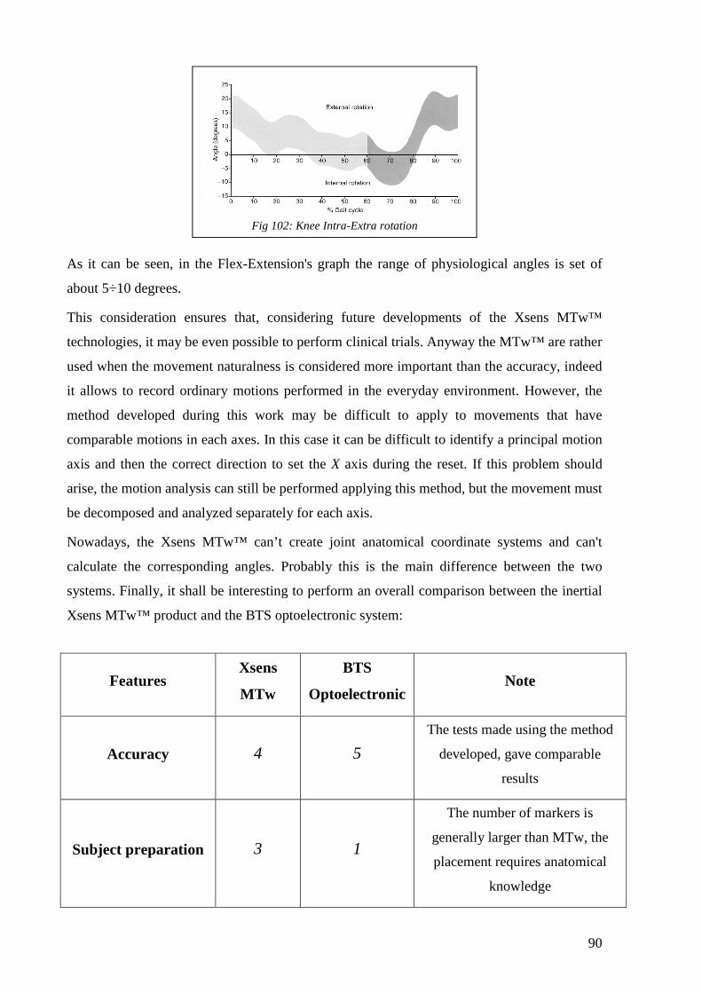
90
Fig 102: Knee Intra-Extra rotation
As it can be seen, in the Flex-Extension's graph the range of physiological angles is set of
about 5÷10 degrees.
This consideration ensures that, considering future developments of the Xsens MTw™
technologies, it may be even possible to perform clinical trials. Anyway the MTw™ are rather
used when the movement naturalness is considered more important than the accuracy, indeed
it allows to record ordinary motions performed in the everyday environment. However, the
method developed during this work may be difficult to apply to movements that have
comparable motions in each axes. In this case it can be difficult to identify a principal motion
axis and then the correct direction to set the X axis during the reset. If this problem should
arise, the motion analysis can still be performed applying this method, but the movement must
be decomposed and analyzed separately for each axis.
Nowadays, the Xsens MTw™ can’t create joint anatomical coordinate systems and can't
calculate the corresponding angles. Probably this is the main difference between the two
systems. Finally, it shall be interesting to perform an overall comparison between the inertial
Xsens MTw™ product and the BTS optoelectronic system:
Features Xsens
MTw
BTS
Optoelectronic Note
Accuracy 4 5
The tests made using the method
developed, gave comparable
results
Subject preparation 3 1
The number of markers is
generally larger than MTw, the
placement requires anatomical
knowledge
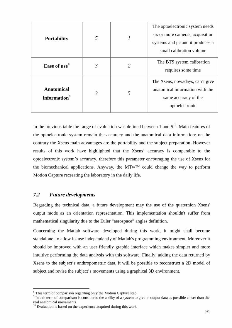
91
Portability 5 1
The optoelectronic system needs
six or more cameras, acquisition
systems and pc and it produces a
small calibration volume
Ease of use8 3 2 The BTS system calibration
requires some time
Anatomical
information 9 3 5
The Xsens, nowadays, can’t give
anatomical information with the
same accuracy of the
optoelectronic
In the previous table the range of evaluation was defined between 1 and 510. Main features of
the optoelectronic system remain the accuracy and the anatomical data information: on the
contrary the Xsens main advantages are the portability and the subject preparation. However
results of this work have highlighted that the Xsens’ accuracy is comparable to the
optoelectronic system’s accuracy, therefore this parameter encouraging the use of Xsens for
the biomechanical applications. Anyway, the MTw™ could change the way to perform
Motion Capture recreating the laboratory in the daily life.
7.2 Future developments
Regarding the technical data, a future development may the use of the quaternion Xsens'
output mode as an orientation representation. This implementation shouldn't suffer from
mathematical singularity due to the Euler “aerospace” angles definition.
Concerning the Matlab software developed during this work, it might shall become
standalone, to allow its use independently of Matlab's programming environment. Moreover it
should be improved with an user friendly graphic interface which makes simpler and more
intuitive performing the data analysis with this software. Finally, adding the data returned by
Xsens to the subject’s anthropometric data, it will be possible to reconstruct a 2D model of
subject and revise the subject’s movements using a graphical 3D environment.
8 This term of comparison regarding only the Motion Capture step 9 In this term of comparison is considered the ability of a system to give in output data as possible closer than the real anatomical movements 10 Evaluation is based on the experience acquired during this work

92
Another next step which can be done regarding the Xsens use, is to get access to all data and
configurations of each MTw, developing a software that fully utilizes the SDK’s capabilities.
The most clinically interesting future development would be to create a method for defining
joint coordinate systems using the Xsens MTw™ product. The method explained in Chapter
6, may be the starting point because the joint coordinate system must be formed by
anatomical rotation axes. The main problem regarding this system is it has not orthogonal
axes, but, once defined, the rotations about these axes are anatomically meaningful. This
approach, in addition to being an important step for Xsens motion analysis applications, might
decrease the larger difference of diffusion between Xsens inertial sensor and
stereophotogrammetric system.

93
CHAPTER 8
Bibliography
8.1 Ringraziamenti
Ringrazio innanzitutto mio padre,mia madre e mia sorella per avermi dato l’opportunità di
raggiungere questo importante traguardo. Senza il loro continuo sostegno, il cammino fin qui
percorso sarebbe stato infinitamente più complicato.
Un sentitissimo ringraziamento va ai miei nonni, che, senza bisogno di parole,
quotidianamente mi rendono felice.
Ringraziare Anita sarebbe quantomeno riduttivo, inutile dire che in ogni momento di questi
“quasi” quattro anni è sempre stata al mio fianco. Se non mi avesse dato la spinta necessaria
al momento delle preimmatricolazioni, probabilmente avrei preso strade diverse; mi ha reso
consapevole delle varie possibilità che era possibile intraprendere, credendo in me più di
quanto non facessi io stesso.
Un enorme ringraziamento “collettivo” va a tutti i miei familiari, parenti e persone a me care,
per il sostegno e l’affetto dimostratomi. Un “grazie” particolare va a Mosè, il quale mi ha
sempre sostenuto e capito nei momenti più duri.
Imperdonabile sarebbe non rivolgere un sentito ringraziamento a tutti i ragazzi conosciuti fin
qui, con i quali sono state condivise innumerevoli esperienze che sicuramente ci hanno aiutato
a crescere e a maturare.
Un ringraziamento speciale va ai “più intimi” compagni di avventure, sia storici che
conosciuti durante questi anni: Alex, Mattia, Michael, Riccardo, Andrea, Filippo, Sofia,
Nicola e Paolo. Di questi ringrazio in particolar modo chi mi ha aiutato e mi è stato vicino
(non strettamente in ambito didattico questo ultimo mese.
Un ringraziamento per l’enorme pazienza avuta è necessario nei confronti delle co-animatrici
e del don.

94
Vorrei infine ringraziare il Prof. Petrone Nicola, il Dr. Marcolin Giuseppe, l’Ing. Giubilato
Federico e tutti i ragazzi del Laboratorio di Costruzioni Meccaniche del DIM per avermi
concesso l’opportunità di eseguire questo progetto, per il continuo supporto avuto e per tutte
le nuove cose che ho avuto modo di imparare.
8.2 Bibliography
Wu G. and Cavanagh P.R. (1995), ISB recommendations for standardization in the reporting of kinematic data. Journal of Biomechanics 28, 1257-1261 (2002), ISB recommendation on definitions of joint coordinate system of various joints for the reporting of human joint motion – part I: ankle, hip and spine. Journal of Biomechanics 35, 543-548 Wu G, van der Helm F.C.T., (DirkJan) Veeger H.E.J., Makhsous M, Van Roy P, Anglin C, Nagels J, Karduna A. R., McQuade K., Wang X.,Werner F.W., Buchholz B (2005), ISB recommendation on definitions of joint coordinate system of various joints for the reporting of human joint motion – part II: shoulder, elbow, wrist and hand. Journal of Biomechanics 38, 981-992 Cappozzo A., Catan A., Della Croce U., Leardini A., (1995), Position and orientation in space of bones during movement: anatomical frame definition and determination. Clinical Biomechanics 10, 171-178 Cappozzo A., Catan F., Leardini A., Benedetti M.G., Della Croce U., (1996), Position and orientation in space of bones during movement: experimental artefacts. Clinical Biomechanics 11, 90-100 Cappello A., Cappozzo A., La Palombara P.F., Lucchetti L., Leardini A., (1997), Multiple anatomical landmark calibration for optimal bone pose estimation. Human movement science 16, 259-274 Cappozzo A., Della Croce U., Leardini A., Chiari L., (2005), Human movement analysis using stereophotogrammetry Part I: theoretical background. Gait and Posture 21, 186-196 Della Croce U., Leardini A., Chiari L., Cappozzo A., (2005), Human movement analysis using stereophotogrammetry Part 4: assessment of anatomical landmark misplacement and its effects on joint kinematics. Gait and Posture 21, 226-237 Cappello A, Cappozzo A, La Palombara P. F., Lucchetti L, Leardini A, (1997), Multiple anatomical landmark calibration for optimal bone pose estimation. Human Movement Sience Cutti A. G., Giovanardi A., Rocchi L., Davalli A., Sacchetti R.(2008), Ambulatori measurement of shoulder and elbow kinematics through inertial and magnetic sensors. Med Bio Eng Comput 46, 169-178 AIS Lab, Università degli studi di Milano, 2007. Mtw User Manual, © Xsens Technologies B.V. M. J. Roberts, Signal and Systems. McGraw Hill Vaughan C.L., Davis B.L., O’Connor J.C. “Dynamics of Human Gait”, Second Edition. Kiboho Publishers, Cape Town, South Africa. J. Richards. “Biomechanics in Clinic and Research”, Churchill Livingstone, Elsevier, 2008.

95
Human movement analysis using stereophotogrammetry.Part 1: theoretical background, Aurelio Cappozzo et Al., Gait and Posture 21 (2005) 186–196.
8.3 Webography
http://www.motion-capture-system.com/resources/history.html http://www.kingston.gov.uk/browse/leisure/museum/collections/muybridge/about_muybridge.htm http://www.ctie.monash.edu.au/hargrave/marey.html http://web.mit.edu/invent/iow/edgerton.html http://accad.osu.edu/~bwindsor/AC694Z_Spring2004/Class1_brian_bw.pdf http://www.bium.univ-paris5.fr/marey/ http://www.dartfish.com http://www.arielnet.com/start/ http://www.btsbioengineering.com http://mafija.fmf.uni-lj.si/seminar/files/2007_2008/MEMS_accelerometers-koncna.pdf http://www.engineerguy.com/bio.htm http://labspace.open.ac.uk/mod/resource/view.php?id=420014 http://www.pyroelectro.com/tutorials/accel_intro/ http://clifton.mech.northwestern.edu/~me381/project/done/Gyroscope.pdf http://www.sensorsmag.com/sensors/acceleration-vibration/an-overview-mems-inertial-sensing-technology-970 http://embeddedsystemnews.com/stmicroelectronics-introduces-a-new-family-of-single-and-multi-axis-mems-micro-electro-mechanical-systems-gyroscopes.html http://www.motion-capture-system.com http://www.xsens.com/en/company-pages/company/human-mocap http://www.shoppingtrolley.net/anatomy-and-physiology-2b.shtml
http://www.btsbioengineering.com/
"Virtual Figure Drawing Studio (Male) 1.08a" is the software used to create the figure 24, 25, 26 and 27.