UNIVERSITÉ DE MONTRÉAL

DATA ANALYSIS FROM AN INTERNET OF THINGS SYSTEM IN A GAS STATION

CONVENIENCE STORE

GEORGES NASSIF

DÉPARTEMENT DE MATHÉMATIQUES ET DE GÉNIE INDUSTRIEL

ÉCOLE POLYTECHNIQUE DE MONTRÉAL

MÉMOIRE PRÉSENTÉ EN VUE DE L’OBTENTION

DU DIPLÔME DE MAÎTRISE ÈS SCIENCES APPLIQUÉES

(GÉNIE INDUSTRIEL)

JUILLET 2018

© Georges Nassif, 2018.

UNIVERSITÉ DE MONTRÉAL

ÉCOLE POLYTECHNIQUE DE MONTRÉAL

Ce mémoire intitulé :

DATA ANALYSIS FROM AN INTERNET OF THINGS SYSTEM IN A GAS STATION

CONVENIENCE STORE

présenté par : NASSIF Georges

en vue de l’obtention du diplôme de : Maîtrise ès sciences appliquées

a été dûment accepté par le jury d’examen constitué de :

M. DANJOU Christophe, Doctorat, président

M. ARMELLINI Fabiano, D. Sc., membre et directeur de recherche

M. ROBERT Jean-Marc, Doctorat, membre

iii

DEDICATION

Dédié à ma famille qui a été mon support durant tous mes années d’éducation.

iv

RÉSUMÉ

Le numérique est de plus en plus populaire et peut être appliquée à plusieurs industries et

entreprises afin d'améliorer la productivité et extraire des informations de marketing. Ce travail de

recherche s’adresse sur le potentiel des applications d'exploration de données dans un magasin

numérisé de vente au détail traditionnel. L'objectif est de démontrer que grâce à un système IoT,

des informations peuvent être extraites à partir des données collectées à l'aide des méthodes

appropriées, tel que les méthodes d'exploration de données. Nos objectifs ont été réalisés en

installant des capteurs Bluetooth dans un dépanneur de station d’essence dans la ville de Laval et

en recueillant des données provenant des appareils Bluetooth des clients. Ces appareils incluent

tous les téléphones intelligents et les montres intelligentes équipés de la technologie Bluetooth.

Une collecte automatisée a été faite sur une durée de une semaine. À partir des données collectées,

une première analyse a été effectué pour trouver une corrélation entre le RSSI et les distances

réelles dans le but de tracer le mouvement des clients dans le magasin. Ces analyses ont montré

que la précision des capteurs n’est pas assez forte pour démontrer un mouvement précis des clients.

Pour s’adapter au manque de précision observé, la prochaine étape a été de regarder les données

des capteurs comme des événements de présences ou absences dans les zones autours de chaque

capteur. Avec les présences identifiées, une proportion de volume d’activité dans chaque zone a

été établi comme donnée pour être utilisée avec les rapports de ventes du magasin pour en

construire un arbre de décision. Nos résultats ont démontré que des informations peuvent être

extraites à partir de la construction de ces arbres de décision qui contiennent des données venant

d'un système IoT bien mis en place dans un environnement de vente au détail traditionnel.

v

ABSTRACT

Digitalization is increasingly popular and can be applied to multiple industries and businesses to

improve productivity and extract marketing insights. This research work looks at the potential of

data mining applications in a digitalized traditional retail store. The goal is to demonstrate that

through the means of an IoT system, insight can be extracted from the collected data with the proper

tools, such as data mining methods. This has been done by installing Bluetooth beacons in a gas

station convenience store in the city of Laval and collecting data coming from the customers

Bluetooth devices. These devices include all smartphones and smart watches equipped with

Bluetooth. An automated collection of data was done for a duration of one week. From the collected

data, a first analysis was done to find a correlation between the RSSI and real distances to trace

customers pathways within the store. These analysis showed us that the sensors precisions are not

high enough to show a precise client pathway within the store. To adapt to this lack of precision,

the next step was to look at the data from the sensors as events of presences or absences in the

zones around each sensor. With each presence identified, a proportion of volume of activity in each

zone has been established as data to be used with the store’s sales report to build a decision tree.

Our results have showed that useful information can be extracted from a properly constructed

decision tree with data coming from an IoT system put in place in a traditional retail environment.

vi

TABLE OF CONTENTS

DEDICATION .............................................................................................................................. III

RÉSUMÉ ....................................................................................................................................... IV

ABSTRACT ................................................................................................................................... V

TABLE OF CONTENTS .............................................................................................................. VI

LIST OF TABLES ..................................................................................................................... VIII

LIST OF FIGURES ........................................................................................................................ X

LIST OF SYMBOLS AND ABBREVIATIONS.......................................................................... XI

LIST OF APPENDICES ..............................................................................................................XII

CHAPTER 1 INTRODUCTION ............................................................................................... 1

1.1 Thesis structure ................................................................................................................ 3

CHAPTER 2 IOT AND DATA MINING OVERVIEW .......................................................... 4

2.1 Internet of Things (IoT) .................................................................................................... 4

2.1.1 Definition ..................................................................................................................... 4

2.1.2 Technologies ................................................................................................................ 5

2.1.3 Applications in Brick & Mortar Retail ......................................................................... 7

2.1.4 Challenges .................................................................................................................... 9

2.2 Data Mining Methods ..................................................................................................... 12

2.2.1 Classification and Regression Methods ..................................................................... 13

2.3 Literary Review Conclusion ........................................................................................... 15

CHAPTER 3 MATERIALS AND METHODS ...................................................................... 16

3.1 Objectives ....................................................................................................................... 16

3.2 IoT system setup ............................................................................................................. 16

3.2.1 Store Identification ..................................................................................................... 16

vii

3.2.2 Technology Identification .......................................................................................... 17

3.2.3 Sensors Setup ............................................................................................................. 18

3.3 RSSI To Real Distances Triangulation Methods ........................................................... 19

3.3.1 Data Collection ........................................................................................................... 19

3.3.2 Zone Definition Triangulation Methods .................................................................... 24

3.4 Sales Data Mining Setup ................................................................................................ 27

3.5 Methods Conclusion ....................................................................................................... 28

CHAPTER 4 RESULTS AND DISCUSSION ....................................................................... 29

4.1 Zone Definition .............................................................................................................. 29

4.1.1 Four-Sensor Triangulation Methods .......................................................................... 29

4.1.2 Single Sensor Zoning ................................................................................................. 39

4.2 Sales & Beacons Data Analysis ..................................................................................... 44

CHAPTER 5 CONCLUSION ................................................................................................. 52

BIBLIOGRAPHY ......................................................................................................................... 54

APPENDICES ............................................................................................................................... 57

viii

LIST OF TABLES

Table 2.1: Smart Objects ................................................................................................................ 11

Table 4.1: Sensor Zones Description ............................................................................................. 19

Table 4.2: RSSI Signals, Fitbit Not on Body [dB] ......................................................................... 22

Table 4.3: RSSI Signals, Fitbit on Wrist [dB] ................................................................................ 22

Table 4.4: RSSI Signals, iPhone X in Front Pocket [dB] .............................................................. 23

Table 4.5: RSSI Signals, iPhone X in Back Pocket [dB] ............................................................... 23

Table 4.6: Distances Between Each Delimitation Point and Beacon [m] ...................................... 24

Table 4.7: Linear Method Slopes [m/RSSI] ................................................................................... 25

Table 4.8: Logarithmic Method Slopes [m/RSSI] ......................................................................... 26

Table 5.1: iPhone X Calculated Distances from Beacons Using Linear Method [m] ................... 31

Table 5.2: iPhone X Distances Experimental Errors with Linear Method ..................................... 31

Table 5.3: Linear Formula Zone Limits in RSSI ........................................................................... 34

Table 5.4: iPhone X Calculated Distances from Beacons Using Log Method [m] ....................... 36

Table 5.5: iPhone X Distances Experimental Errors with Log Method ......................................... 36

Table 5.6: Logarithmic Formula Zone Limits ................................................................................ 37

Table 5.7: Single Sensors Zoning Limits ....................................................................................... 40

Table 5.8: Number of Presences Per Beacon ................................................................................. 42

Table 5.9: Classification Logic for Sales Proportions and Beacon Activity .................................. 42

Table 5.10: Presence at Beacons (Per Day Proportions) ................................................................ 43

Table 5.11: Presence at Beacons (Per Beacon Proportions) .......................................................... 43

Table 5.12: Presence at Beacons (Per Day Relative Proportions) ................................................. 43

Table 5.13: Sales Proportions Per Category (For the Week) ......................................................... 45

Table 5.14: Sales Proportions Relative to The Week ..................................................................... 45

ix

Table 5.15: Sales Proportions Relative to The Categories ............................................................. 45

Table 5.16: Dataset 1 Using Table 5.11 and Table 5.14 ................................................................ 46

Table 5.17: Dataset 2 Using Table 5.11 And Table 5.15 ............................................................... 46

Table 5.18: Dataset 3 Using Table 5.12 Table 5.14 ....................................................................... 46

Table 5.19: Dataset 4 Using Table 5.12 Table 5.15 ....................................................................... 47

Table 5.20: Dataset 1 Prediction Accuracy .................................................................................... 47

Table 5.21: Dataset 2 Prediction Accuracy .................................................................................... 48

Table 5.22: Dataset 3 Prediction Accuracy .................................................................................... 48

Table 5.23: Dataset 4 Prediction Accuracy .................................................................................... 48

Table 5.24: Decision Tree Legend ................................................................................................. 49

Table 5.25: Dataset 4 Classified Values ......................................................................................... 49

x

LIST OF FIGURES

Figure 2-1: Decision Tree Example ............................................................................................... 13

Figure 4-1: Pareto Main Page User Interface ................................................................................. 17

Figure 4-2: RFID Sensors Locations .............................................................................................. 18

Figure 4-3: Zone Delimitation Captures ........................................................................................ 21

Figure 5-1: Defined Zones for Pathway Tracing ........................................................................... 30

Figure 5-2: Actual Pathway Taken with The Fitbit ........................................................................ 32

Figure 5-3: Demonstration of RSSI Limit per Zone ...................................................................... 33

Figure 5-4: Pathway Detected Using Linear Correlation ............................................................... 35

Figure 5-5: Pathway Detected Using Logarithmic Correlation ..................................................... 38

Figure 5-6: Single Sensors Zoning ................................................................................................. 40

Figure 5-7: Alcoholic Drinks from Dataset 4 Decision Tree ......................................................... 50

xi

LIST OF SYMBOLS AND ABBREVIATIONS

ARAT Active Reader Active Tag

ARPT Active Reader Passive Tags

BLE Bluetooth Low Energy

CART Classification and Regression Trees

IoT Internet of Things

ISO International Organization for Standardization

GPS Global Positioning System

M2M Machine to Machine

MAC Media Access Control

NFC Near Field Communication

PRAT Passive Reader Active Tag

RFID Radio Frequency Identification

RSSI Received Signal Strength Indicator

V2V Vehicle to Vehicle Communication

xii

LIST OF APPENDICES

APPENDIX A – PARETO DATA COLLECTION CODES ........................................................ 57

APPENDIX B – RAW DATA ....................................................................................................... 59

APPENDIX C – PYTHON CODES .............................................................................................. 63

APPENDIX D – DECISION TREES ............................................................................................ 79

1

CHAPTER 1 INTRODUCTION

Technology is now at the forefront of all business innovations and retail stores must adapt to that

reality. IoT applications are increasingly popular and can lead to significant revenue improvements

when properly implemented. This research project will attempt to further advance methods to work

towards that new reality. The Internet of Things (IoT) and data mining are concepts we hear more

and more about but are not always well understood. The technical definition for IoT, as defined in

The Internet of Things: A survey, consists of a “pervasive presence around us of a variety of things

or objects […] which are able to interact with each other and cooperate with their neighbours to

reach common goals” (Atzori et al., 2010). These interactions are done through means of wireless

communications technologies such as Radio-Frequency Identification. In practical terms,

connected objects can constantly communicate with each other sending all sorts of information

such as physical position, transactions information and other (Atzori et al., 2010). Data mining,

which will be explored furthermore in this research paper, can be briefly defined as “the discovery

of interesting, unexpected or valuable structures in large datasets” as defined by Hand (2007).

These two concepts of IoT and data mining are closely interlinked together. With well-designed

IoT systems, we can have useful data mining applications. These can be adopted in the context of

the retail industry to dramatically revolutionize the way the merchant and customers interact with

each other in a brick and mortar store.

According to a web page article from Forbes1, 70% of retail executives say that they are ready to

adopt IoT for a better customer experience and 73% agree that proper management of that data is

critical to their operations (Columbus, 2017). These implementations can be on applied on various

facets of the industry such as brick and mortar store layouts or a customer in-store personalized

experience amongst other applications. That same article also highlights retailer readiness with a

statistic showing that 79% of retailers will be ready by 2021 to offer each unique customer a

personalized in store experience using IoT technologies (Columbus, 2017).

Articles published by technology and management consulting firms Accenture and McKinsey

highlights the disruption potential the IoT will have in the retail industry (Gregory, 2014). Several

1https://www.forbes.com/sites/louiscolumbus/2017/03/19/internet-of-things-will-revolutionize-retail/%20-%2056d24b785e58

2

areas where there is room for improvements are identified, but for the scope of this project, our

research project will focus on improving customer experience. Some degree of personalized

marketing already widely exists. For example, when shopping for a baby chair on Amazon, ads of

baby cradles and other baby related furniture will start appearing on the user’s Facebook account.

The Internet of Things is identified as taking a step further, where with object interconnectivity the

business can predict the consumers’ needs by observing their habits, and collecting and analysing

several data points coming from consumer’s smartphones or smart wearables (Gregory, 2014). IoT

has the potential to improve customer relationship management tools by building a real-time and

personalized profile on each consumer, solely using technology with no human objectivity. For

example, a customer that walks into the store is identified by his phone and then notified to an in-

store promotion which is only directed towards him based on his browsing history, or from any

other source of data collected (Manyika et al., 2015). Another identified IoT application is the

optimization of the store layout based on consumers’ location. For example, high margin products

can be placed in areas where a high flow of traffic is recorded from the sensors (Gregory, 2014).

Data collected from IoT devices comes to little use as it is without any proper analytics tool. Data

mining serves as a tool to make sense of structured and unstructured data. Aligned with this

research project, data mining is frequently used to analyse customer’s habits for marketing

purposes by using methods such as classification, clustering and decision trees. It is important to

note that the literature stresses the point that an effective data mining process does not solely rest

in the data mining method, but firstly in a proper judgement of the business application of the data

(Radhakrishnan et al., 2013).

This project is done in partnership with a gas station convenience store based in Laval, Quebec,

which is looking to explore how IoT applications can improve its business operations. The focus

of this project will not be on the conceptual system required for IoT implementation, but instead

on demonstrating how data coming from a properly implemented system can be exploited to bring

useful insights for operational and marketing purposes. To be able to extract useful information

from the IoT system, data mining will be used for the data analysis. Data mining methods, which

will be explored in more depth in chapter 2, permit us to easily analyse large datasets which would

otherwise be difficult to interpret.

3

1.1 Thesis structure

This thesis is structured as follows. Chapter 2 presents a literature review of IoT, more precisely

the definition of IoT, its technologies, its use in brick and mortar retail and its challenges. We will

also discuss in chapter 2 some data mining techniques which are pertinent to IoT systems and

marketing. Chapter 3 will present the research objectives in depth as well as the methods that have

been used to conduct the experimentations. The methods include store and technology

identification, data collection steps and data analysis methods. Chapter 4 will present a detailed

analysis and discussion of the results obtained from the data collection done in this research.

Chapter 5 will present conclusions and recommendations for future advancements in this research

and discuss limitations.

4

CHAPTER 2 IOT AND DATA MINING OVERVIEW

This research project will involve setting up an IoT system within a retail store environment and

perform pertinent data analysis on the collected data. Before doing so, this chapter will start with

presenting a literature review on the work done related to IoT systems and their technologies, as

well as their applications and challenges. The second part of this literature review will look at the

data mining methods which are pertinent to be applied on the collected data coming from customers

at a convenience store.

2.1 Internet of Things (IoT)

2.1.1 Definition

One of the first mentions of internet of things originated from Kevin Ashton back in 1999 (Ashton,

2009). He points out the overwhelming presence of data sources which are limited by one major

limitation: the human factor in the capturing process. From there was born the idea of IoT,

computers that would replace bar code scanners and such capture a continuous and complete set of

data. Technologies RFID (Radio Frequency Identification) and sensors have permitted IoT to

develop.

IoT is a vast term which can vary in definition, but essentially converges to a fundamental definition

where it consists of a connected system of smart objects, which work together and with little to no

human interventions, to supply us with information that we want (Perera, Zaslavsky, Christen, &

Georgakopoulos, 2014).

Amongst the definitions of IoT, we find in literature some definitions that focus on the “Things”,

some that focus on the “Internet” and some on the semantics of the “Internet of Things”.

The definition that focuses on the “Things” studies the integration of objects into a network by the

use of technologies such as RFID (Bandyopadhyay & Sen, 2011). To be a “thing” in an IoT system,

that device must have the capacity to collect data without any human interventions (Gubbi, Buyya,

Marusic, & Palaniswami, 2013). Further in the literature review in section 2.1.4.2 some

characteristics of these smart objects will be discussed in greater details.

The other focus is on the “Internet” which is on a higher-level approach that looks at the network

and not at the individual objects (Bandyopadhyay & Sen, 2011).

5

The third focus is on the semantics of the “Internet of Things. This approach aims to consolidate

the various challenges pertaining to data collected in this IoT network. These challenges include

the collection of data, storage and analysis amongst others (Bandyopadhyay & Sen, 2011).

2.1.2 Technologies

As it will be seen a bit later in this research paper in

Table 2.1, for an IoT system to be effective, the smart objects within it must be process-aware

objects, that is, objects that can discern activities in relation to location and time (Palumbo,

Barsocchi, Chessa, & Augusto, 2015).

Indoor localization has its own set of challenges which is not present in outdoor localization

technologies such as GPS. Some challenges include indoor obstructions that would disrupt

Bluetooth signal. Other challenges are the interference with other wireless signals in an indoor

space that might interfere with signal strengths (Chawathe, 2008).

IoT technologies can be found in literature under categories such as RFID, NFC (Near Field

Communication), M2M (Machine to Machine) and V2V (Vehicle to Vehicle Communication).

RFID works with the use of electronic tags attached to the tracked items which communicate with

the receivers through radio frequency electromagnetic fields. The tags can either be PRAT (Passive

Reader Active Tags), ARPT (Active Reader Passive Tags) or ARAT (Active Reader Active Tag).

NFC technologies comprise RFID technologies but are found within mobile phones to enable

communications between them. These technologies work on very short range and can only transfer

a small amount of data. The next category is M2M and enables communication between a variety

of electronics such as computers, smart phones and sensors. The functioning of M2M is described

as the ability of the device to send requested information to other devices. This is done through

technologies such as Bluetooth and WIFI (Network based) amongst others. The last category is

V2V and comprises applications which are long range. The nodes in a V2V network can

communicate to each other’s within a range of 100m. This is done with an Ad-Hoc network

comprised of connected sensors (Shah & Yaqoob, 2016).

For this research project, the category of interest is M2M technologies which are the most readily

accessible, hence this literature review will focus on Bluetooth and WIFI sensors as they are the

most easily purchasable for our research.

6

2.1.2.1 Bluetooth Sensors

Bluetooth was conceived in 1994 and serves as a mean of device short range communications

without the need of physical cables. It works with a radio system and is present in many electronic

devices such as computers or printers (Ferro & Potorti, 2005).

Since this wireless mean of communication has started in 1994, Bluetooth technologies have

evolved in a significant way to become highly effective in indoor localization applications. The

emergence of BLE from standard Bluetooth is enabling low-powered short range communication

and faster transmission of data. It has been implemented since its evolution in the majority of smart

devices (Gomez, Oller, & Paradells, 2012). BLE technology also has many practical advantages

such as not requiring a large setup space, compatible with multiple Bluetooth enabled devices and

highly power efficient (Zhuang, Yang, Li, Qi, & El-Sheimy, 2016). An experimental setup was

found in the literature where the experiment was set up in an office space with eight BLE devices

to validate the use of this technology. The sensors were placed at a level 3 m above ground level

in a 6x6 m office. The sensors being place at a high level were unobstructed by office objects such

as desks or cubicles. A localization method was established using the sensor’s RSSI (Received

Signal Strength Indicator), which is simply the measure strength of the captured signal in decibels,

and a logarithmic function determined by equation (1) (Palumbo et al., 2015).

𝑅𝑆𝑆𝐼 = −(10𝑛 ∙ 𝑙𝑜𝑔10𝑑 − 𝐴) (1)

Where n is the slope distance/RSSI, A is the intersection in RSSI and d is the distance. The data

collection was done with a person walking with a phone put 1.5 m above ground level, and stopping

five seconds at marked locations. After using the above formula to establish a correlation between

RSSI and distance, results found that 75% of the calculated distances versus real ones were within

1.8 m of reality (Palumbo et al., 2015).

Some advantages of Bluetooth technology will be discussed. Among the strength of BLE

enumerated in the beginning of this section, that technology is energy efficient and highly

compatible with multiple devices. This advantages permits BLE sensors to be installed with

batteries, instead of being hardwired, increasing their mobility (Zhuang et al., 2016).

BLE does come with some disadvantages. One of them is the range is limited, resulting in having

to deploy multiple sensors to achieve a complete coverage of a larger space. Although literature

7

also describes it as a potential advantage in some situations. With a limited range, if a device is

captured on the sensor we are guaranteed that it is in an area at a proximity of the BLE beacon.

Another disadvantage is the time it takes for a Bluetooth device to be discovered. In an

experimentation done by Chawathe, it was found that it took on average a time of 10.24 seconds

for BLE sensor to successfully capture the presence of a Bluetooth device (Chawathe, 2008).

2.1.2.2 WIFI Sensors

Another technology with big potential in indoor localization applications are WIFI enabled sensors.

WIFI has many advantages, such as the technology already being implemented in most mobile

devices and now even in larger electronics such as smart TVs and cars. To add more advantages,

WIFI devices are also not power hungry. Although, WIFI equipped beacons require more energy

than their BLE counterparts making them less versatile. An advantage of WIFI technologies is

identification. WIFI protocols are more accurate in identifying the scanned device then Bluetooth

technologies (Saloni & Hegde, 2016).

Other characteristics of WIFI have also been found in literature which explains the technologies

popularity in IoT systems. WIFI enabled sensors have the ability to transfer a high amount of data

at very high speeds which is essential for data collection. It has also been identified as having a

high coverage area of about 300 m outdoors and 100 m indoors. The technology can also

accommodate a growing system since it is easily scalable. Finally, another interesting aspect of

WIFI is the reliability of its signal (Li, Xiaoguang, Ke, & Ketai, 2011).

An important aspect of WIFI technology is in relation with a device’s MAC Address. A MAC

Address is a unique identifier which is seen by the network the device is connected on. A WIFI

connected device will have a unique MAC Address which permits unique identification. This

means that in an IoT system a particular device can be identified and studied over time (Cunche,

2014).

2.1.3 Applications in Brick & Mortar Retail

IoT applications in brick and mortar retail stores are still relatively new since sensors have only

become recently affordable and the adoption of this technology is recent. Literature is scarce on

8

the subject but there are still some research applications done in a brick and mortar retail

environment like it is the case of this research project.

An interesting application identified in literature consists of tracking customer’s movements in

store to adapt specific promotions according to the data collected (Hagberg, Jonsson, & Egels-

Zandén, 2017). A study was done in a South Korean retail store to observe customers’ behavior for

marketing purposes (Hwang & Jang, 2017). Their movements were tracked by using IoT sensors

which interact with the customer’s smartphones WIFI antennas, revealing their semi-precise

physical location inside the store. The precision of this technology varies with the quality of devices

which interact with each other and the WIFI antenna signal strength. This leads to a certain margin

of error in the data analysis. Each customer is identified by his unique “Mac Address” from his

smartphone allowing each data point to be linked to a recurrent customer. The data is also temporal

having a time stamp associated with each data point. With the data collected, an analysis was made

to observe how the customers interact with different store items and what their general routine is.

This led to a conclusion showing how varying the location of different displays in store can lead to

an optimized layout for sales. An important remark done by the authors of the experiment is that

although a change of sales and traffic volume was observed after applying the optimized layout,

there is no guarantee that it is the sole cause for that change. Furthermore, other variables were not

taken into effect such as interactions with staff members or cash counter interactions (Hwang &

Jang, 2017).

Another research paper was found with experimentations using NFC equipment. In that study, the

store products as well as its clients are both NFC equipped to start a link between the consumers

and the shop. That link brings forth the possibility of targeted presentations to customers. For

example, a sport loving shopper would see a football game display on the television screen he is

looking at. Another application is to provide a complete shopping package. A customer would

insert his items in his virtual basket within a physical store and in consequence the sales associate

can provide a personalized package related to the items chosen by the customer. This package

would be done automatically using IoT analytics and not simply a subjective assessment (Longo,

Kovacs, Franke, & Martin, 2013).

A study was also found evaluating customer’s behaviors in a digitalized grocery store. The article

explores the potential of embedding the store with smart objects by integrating cell phones with

9

smart equipped baskets, store shelves and products. The study involved sending a sample of 60

people to shop for a BBQ grocery list. Specifically for the salmon, different promotions would

show up on the shoppers’ cell phones to evaluate their decisions to get fresh salmon or not based

on the promotions they see. Since this is all connected to an IoT network, these promotions are

customizable and given in real-time. The conclusion of the study was that according to the

promotion displayed, there was a correlation between the customers decision to purchase fresh

salmon or not (Fagerstrøm, Eriksson, & Sigurðsson, 2017).

Applications in brick and mortar can go beyond the direct customer service experience but also

indirectly by being more efficient in store operations. An example shown in literature describes a

situation where a refrigerator would be part of an IoT network. That refrigerator would have sensors

capable of detecting whether it’s performing at its full capacity. If that device is faulty, an alert

would be sent to store staff in order to service it (Lee & Lee, 2015).

2.1.4 Challenges

The Internet of Things is still a relatively new concept and many challenges are present in its

adoption. Amongst these obstacles lies the lack of standardization for an IoT infrastructure as well

as implementation challenges.

2.1.4.1 Standardization

With a growing number of adoptions of IoT, basic tasks such as data generation and storage have

a need for a standardized model. Per Banafa’s article, four dependant categories are identified in

the process of standardizing IoT practices: platform, connectivity, business model and killer

applications (Banafa, 2016).

First, a platform which can handle data with the use of the appropriate analytical tools. The platform

also englobes user experience such as the interface design and it should have the capability to be

scaled for larger applications (Banafa, 2016).

Secondly, the need for a standardized connectivity baseline should be established for a proper

stream of data and interaction with the established platforms. Connectivity includes aspects such

as how the data is connected. For example, the use of smart wearable devices, smart homes or on

a much larger scale, smart cities (Banafa, 2016).

10

Thirdly, a robust business model. This is important to have all the players involved in an IoT

infrastructure to be invested in the created ecosystem (Banafa, 2016).

The last point mentioned in the article is “killer applications”. Simply put, killer applications

represent the tangible outcome from the collected data and its analysis (Banafa, 2016).

2.1.4.2 Implementation

The other aspect of IoT challenges lies in its implementation.

The concept of IoT is a complex one and it includes a multiple of inter-related systems that need

to properly work with each other. The systems mentioned by Banafa (2016) include sensors,

networks, standards, intelligent analysis and intelligent actions. Sensors are the driving force of an

IoT system. Recent technology advances in that domain have led to much more affordable IoT

equipment making the implementation affordable for smaller players. Networks define how the

sensors interact with each other and the collecting database. Same as with sensors, advances in

technology has allowed for cheaper network maintenance and much faster speeds. Another

implementation step involves looking at standards. Standards are important to regulate how data is

handled over the network and how it is stored. All three of the first processes of implementations

face similar challenges. Security is of the upmost importance given the fact that there is an

extremely huge amount of data being sent and processed across networks. Other challenges include

regulatory issues and optimizing the power consumption of an IoT system. The other aspects of

implementation which are strongly inter-related with each other are intelligent analysis and

intelligent actions. These steps include transforming the collected data into useful and easy to

understand business knowledge and transitioning that knowledge into tangible actions. The

challenges in these implementations are the proper applications of data analytics on IoT data as

well as updating these systems to support a large flux of incoming real-time data (Banafa, 2016).

Other aspects of implementation challenges are also discussed in Kortuem’s et al. (2010) article.

The research question in their article is focused on the interaction between human users and the

smart objects themselves, which are suggested to have these three fundamental characteristics:

activity-aware objects, policy-aware objects and process-aware objects.

Table 2.1 summarizes the article’s description of these characteristics (Kortuem, Kawsar, Fitton,

& Sundramoorthy, 2010).

11

Table 2.1: Smart Objects

Smart Objects Description

Activity-Aware Objects They can discern different activities and the order in which they are

performed. These objects are simply for data gathering.

Policy-Aware Objects They can understand activities in the scope of the policy that has

been programed for the IoT system. Mainly for compliance.

Process-Aware Objects They can discern different activities with relation to the location

they are performed and the time they are performed at.

Another challenge is implementing smart objects while considering the human interactions. Smart

objects by themselves have little added value, but smart objects that are well integrated into an

ecosystem where they interact not only with each other, but also consider the human inputs, and

there lies the implementation challenge (Kortuem et al., 2010).

2.1.4.3 Ethical Issues

Connecting IoT sensors to people’s personally devices brings with it ethical questions. Does the

user still have his privacy? How is that privacy protected with all the data gathering that happens

in an IoT system?

In BLE technologies, one of the reason of its popularity is because it is not invasive of a person’s

personal device. In order to detect a presence, a BLE beacon only needs to detect a Bluetooth

transmission being made without connecting to the device, which would then be intrusive to one’s

privacy (Chawathe, 2008). However, if a device owner’s actions can be linked to another activity

whose identity is disclosed, for example, using a credit card or using a loyalty card (e.g. Petro-

points), that could allow identify the device owner. It should not be done without the informed

consent of the subject. Therefore, when designing an IoT system to collect information about

people’s trends and habits, close attention must be payed to whether the system has potential

privacy risks.

The ethical issue is much more prominent in WIFI driven IoT systems. As previously discussed in

the literature review, we found that WIFI can identify a device’s unique Mac Address. This means

12

that the monitored device owner is being watched and can be profiled and potentially reveals the

person’s personal identity. Another issue is the possibility of linking various WIFI devices to the

same owner which can lead to greater data collection and in return a greater invasion of privacy

(Cunche, Kaafar, & Boreli, 2014).

2.1.4.4 ISO Standardization

To overcome the challenges enumerated in sections 2.1.4.1 and 2.1.4.2, the International

Organization for Standardization published ISO 30141. This standard serves the purpose to provide

the necessary tools for all IoT systems to work with. It helps to overcome the mentioned challenges

by setting the following objectives as stated by the standard: “to enable the production of a coherent

set of international standards for IoT”, “to provide a technology-neutral reference point for defining

standards for IoT” and “to encourage openness and transparency in the development of a target IoT

system architecture and in the implementation of the IoT system” (ISO, 2018).

2.2 Data Mining Methods

Once a proper IoT setup has been done in our gas station convenience store, data mining methods

are going to be used to properly analyze the data collected. The following section will present the

data mining methods which are pertinent to the type of data that we will be collecting for our

research project.

The use of data analytics goes hand in hand with an IoT system. Without these tools, the insight

that can be extracted from the sheer volume of data is very limited (Radhakrishnan et al., 2013).

Data mining methods are plentiful and an extensive literary review can be done on this subject but

for our research project we will focus solely on learning methods. Learning methods can be

separated into two categories: supervised learning and unsupervised learning. Supervised learning

methods consist in predicting an output variable based on input variables. This is done with the use

of training and testing datasets. Supervised learning is separated into classification methods and

regression methods. Unsupervised learning methods consist in having only input variables with no

studied output data. This serves the purpose of figuring out how the data is distributed and

categorized. Unsupervised learning is separated into clustering and association methods

(Brownlee, 2016).

13

The focus of our research is to demonstrate the possibility of useful data analysis from an IoT

system. The discussed methods in this literature review section will be on supervised learning

methods as they are the most pertinent for the type of data we will be gathering in our research.

2.2.1 Classification and Regression Methods

Classification methods are used to classify output variables into pre-defined groups or classes of

attributes. The purpose is to correctly predict to what class or group a studied variable, based on its

attributes, will belong to (Kesavaraj & Sukumaran, 2013). Regression methods are very similar to

clustering methods, with the only difference that the output variables are not pre-defined classes or

categories but real values instead (example: sales amounts in dollars) (Brownlee, 2016).

Classification and regression methods all follow the same two fundamental steps. The first step is

the supervised learning part, where a training dataset is used to create classifying rules. The second

step is the applications of these rules to a testing dataset. The methods used are decision trees, rule-

based methods, memory based learning, neural networks and Bayesian networks (Kesavaraj &

Sukumaran, 2013). For our research, we will focus on decision tree methods.

Decision trees represent a classification model in the form of a tree composed of nodes which look

at an attribute, a decision branch which looks at the value of the attribute and leaf nodes which are

the classification (Kesavaraj & Sukumaran, 2013). For example, a node can be: Exercises a

minimum of 4 times a week, and its subsequent decision branch would be true or false. A leaf node

in that decision tree could be “Healthy”. An example of a decision tree is shown in Figure 2-1.

Figure 2-1: Decision Tree Example

Decision trees are constructed by looking over attributes of a training dataset. The first step looks

at all data at the node. If all variables can be assigned to one class, then it becomes a homogenous

14

leaf node. If not, then a partition is created per attribute. This process repeats until all data are put

in a homogeneous leaf node or there are no more attributes to keep dividing into more nodes.

Pruning methods can also be applied which serve to remove nodes that have little added classifying

relevance to the decision tree (Kesavaraj & Sukumaran, 2013).

The quality of each class, which is the ratio of right decisions/classification over the total sample

number at the node, can be measured in various ways per the decision algorithm used. Some

commonly used algorithms are the CART method or C4.5 method (Kesavaraj & Sukumaran, 2013).

The CART method, which stands for Classification and Association Regression Tree, is used to

construct binary trees, meaning each node splits into two binary decisions true and false. The split

is done based on the twoing criteria, which is a measure of class purity. The subsequent tree is then

pruned using the cost-complexity pruning method. Some advantages of the CART method are that

it can easily handle both regression and classification tasks, it can easily determine which variables

are most significant and prune less useful variables. Some disadvantages are that the CART method

can only split one variable at a time at each node and if wrong modifications are done to the training

dataset, it could lead to an unstable tree (Singh & Gupta, 2014).

The C4.5 method starts by finding from all possible splitting tests the one that gives the best result

using the information gain criteria. An important difference between C4.5 and the CART method

is the ability for C4.5 to create a decision tree which contains both discrete and continuous values.

When sorting discrete attributes, a test is used to generate possible outcomes based on the number

of unique attributes for the value at the node. For continuous attributes, the data is split using binary

cuts and the information gain criteria is applied to produce the next node of the decision tree,

similarly to discrete values. C4.5 also allows for pruning by using an error based pruning method.

An advantage of this method includes the ability to sort through both discrete and continuous

attributes. Another advantage is for the method’s capability to leave marked unknown attributes

which will not be calculated in the information gain. A disadvantage of this method is the frequent

generation of nodes with zero or near zero values. This leads to a noisier decision tree with

confusing rules generation (Singh & Gupta, 2014).

An example of supervised learning in literature was found where a study was done in the banking

industry. The article shows how classification analysis can be used to identify the success factors

in direct marketing campaigns. The conclusion of the study was that the duration of the calls and

15

the month of the year the call was made where the biggest contributors to a successful marketing

campaign. This was obtained by applying classification methods on the studied dataset (Moro,

Laureano, & Cortez, 2011).

2.3 Literary Review Conclusion

Chapter 2 presented an overview of the IoT technologies that can be used for remote identification,

such as BLE or WIFI, as well as some applications in retail stores. It also presented the challenges

facing IoT system such as ethical issues that might arise form one. The chapter also presented data

mining concepts which are needed to reveal hidden patterns from the data collected from an IoT

system. These concepts had to be reviewed to understand the objectives which will be listed in the

next chapter.

16

CHAPTER 3 MATERIALS AND METHODS

3.1 Objectives

The objective of this research project is to demonstrate that through the means of an IoT system,

insight can be extracted from the collected data with the proper tools, such as data mining methods.

We built a database which includes Bluetooth devices addresses, RSSI, device classification and

sales figures. This was done using of BLE sensors, tracking the positional and temporal data from

Bluetooth devices and the sales report data coming from the store management.

Using the above data as inputs and studied variables, we will be working towards an analysis for:

- Defining a correlation between device signal strength and physical location of the device

to establish a customer pathway and the amount of customer activity in defined zones.

- Establishing a correlation between the data collected with the IoT sensors and the sales data

using data mining techniques.

The next section will present the methods and experimental procedure used to accomplish the

objectives set above. This research was done in cooperation with Marques’ (2018) research.

Marques’ project focuses on the implementation and conception of an IoT system, whereas this

research focuses on the applications from the data generated. The methodology is separated in

three sections. The first section presents the IoT system setup which was done in cooperation with

Marques. The second section presents the RSSI to real distances triangulation methods used for

customer pathway tracing. The third section presents the data mining method used to analyse the

data coming from the implemented IoT system and the sales report from the convenience store.

3.2 IoT system setup

This sub section presents the store and technology identification for our IoT system setup as well

as the location of our sensors and a description of the products contained in their surrounding areas.

3.2.1 Store Identification

The first step towards accomplishing the goals of this research project is to identify a convenience

store to work with to install sensors and collect data from. Our aim was to find a gas station which

17

has a constant client flow and a regular customer base. This rules out gas stations on the highway

which would include a larger proportion of people traveling. We settled on a convenience store

located in the suburbs of Montreal which is known to have regular customers that go weekly at the

gas station. It is also not by a highway so the proportion of irregular travelers is small.

3.2.2 Technology Identification

As seen in the literature review, many technologies exist for the sake of IoT data collection. For

our experimental setup, we have adopted the solution developed by the Montreal startup

reelyActive2, which provides Bluetooth beacons that continuously collect data from any detected

Bluetooth source. The company also provides an online platform (Pareto), which offers tools to

monitor the status of the beacons and to consolidate data collection. Figure 3-1 shows a Print Screen

from Pareto.

Figure 3-1: Pareto Main Page User Interface

As previously discussed, Bluetooth is a cheap and easy way to collect data from customers while

simultaneously preserving their privacy, and it fitted the modest budget we had for this pilot

project. To stress the ethical question around data collection from personal devices, as discussed

2 http://www.reelyactive.com/

18

in section 2.1.4.3, the data collected was not linked with any identification method such as

payments at the cash or association with a customer’s loyalty card. The company we worked with

also did not disclose any customer information to us. Given these facts, the data we collected was

completely untraceable to any customer. For this reason, we have purchased four Pareto beacons

and a trial subscription of Pareto to access all data collected by the sensors. Costs cannot be

disclosed in this paper to respect the ReelyActive company’s confidential pricing plan given to us.

3.2.3 Sensors Setup

To maximise the quality of the data, zones of interest were identified to insert the RFID beacons

in. These four zones contain products of interest for a data analysis. A detailed description of the

zone contents is shown in

Table 2.1. The sensors located on a scaled map of the store floor are shown on Figure 3-2. The

dark grey bands at the bottom of Figure 3-2 are the store counters.

Figure 3-2: RFID Sensors Locations

19

Table 3.1: Sensor Zones Description

Sensor Label Zone Contains

1 Cash Cash, gum, sweets, tobacco

2 Washroom Lottery, milk, restroom, energy drinks, dairy products, soft

drinks

3 Liquor Alcohol, small electronics, beef jerky, chips, chocolate bags,

mixed nuts

4 Outdoor Ice cream, cold non-alcoholic drinks

As seen in the literature review, ideally the sensors should have been installed high up on the ceiling

to not have signal interference coming from the shelves, but due to store limitations and other

concerns such as theft, the sensors had to be installed in locations that were not free of all

obstructions. Another limitation we had with sensor location was that they had to be placed out of

sight. This was because the company did not want their customers to think that they were in

partnership with the beacon provider ReelyActive. Sensor 1 was installed atop a television facing

the cash. Sensor 2 was installed behind the lottery booth. Sensor 3 was installed on a shelf corner.

Sensor 4 was installed behind a wine fridge. Due to the mentioned limitations, these sensors all had

physical obstructions such as sensor 1 having a TV in the way, or sensor 3 having the lottery booth

in the way.

3.3 RSSI To Real Distances Triangulation Methods

This section presents the data collection performed from the previously set up IoT system as well

as the methods used to find a correlation between measure RSSI values and real physical distances.

3.3.1 Data Collection

A total of three automated data collections as well as one manual data collection were performed

to collect the data for our experimentations.

3.3.1.1 First Raw Data Run

The first raw data run was done for a week using a JavaScript code provided from Pareto. The

collection was done for the duration of one full week. A total of 917493 lines of data were collected

20

during this week. The raw data was stored in an Excel file in CSV format. The pertinent raw data

collected included:

- Timestamp (Epoch format)

- Session duration (milliseconds)

- Device Bluetooth ID

- Device tag

- Strongest RSSI captured with the beacon identified

The code can be found in Appendix A, first section. A sample of the first raw data run can be found

in Appendix B, first section.

After considering the data collected in this data run, we concluded that we would need signal

strengths from each of the beacon at the same time to define zones to trace a customer pathway.

No further analysis was done with this first data run.

3.3.1.2 Second Raw Data Run

A second raw data run was done to include the RSSI captured from each beacon to define more

precise zones by finding the intersecting zone between the four beacon RSSI strengths. The

collection was done for the duration of one full week. A total of 937245 lines of data were collected

during this week. The pertinent data collected is the same as section 3.3.1.1.

The code can be found in Appendix A, second section. A sample of the first raw data run can be

found in Appendix B, second section.

3.3.1.3 Manual Data Run for zone Delimitations

To establish the limits of the store as well as collecting data for the RSSI to physical distances

correlation methods, a manual data run was performed at the convenience store. The RSSI values

at the points identified in Figure 3-3 were collected.

21

Figure 3-3: Zone Delimitation Captures

Using a Fitbit Bluetooth wearable device, trademark of Fitbit Inc., the manual collect was done by

using the Pareto interface and standing for at least 1 min at each of the map positions to stabilize

the RSSI. One run was done with the Fitbit not on a wrist but left sitting on a high object in the

store (Fitbit not on body). Another run was done with the Fitbit on the wrist. Another run was done

with an iPhone X, trademark of Apple Inc., in the front pocket and finally a fourth run was done

with the same phone in the back pocket. The RSSI recorded for each of the four runs is shown in

Table 3.2, Table 3.3, Table 3.4 and Table 3.5. In these tables, the numbers are in RSSI. A higher

RSSI means a closer distance from the beacon and a lower RSSI distance means a further distance

from the beacon. The highest value that was recorded was an RSSI of 182 when a device was

placed directly on a beacon. This value of 182 was found using the online Pareto interface.

22

Table 3.2: RSSI Signals, Fitbit Not on Body [dB]

Table 3.3: RSSI Signals, Fitbit on Wrist [dB]

23

Table 3.4: RSSI Signals, iPhone X in Front Pocket [dB]

Table 3.5: RSSI Signals, iPhone X in Back Pocket [dB]

3.3.1.4 Third Raw Data Run for RSSI to distance validation

For validation purposes, another collect was done using the Pareto code and the Fitbit device.

Referring to Figure 3-3, a path starting from point 1 through point 11 and ending at point 10 was

taken. The Fitbit device was placed at each point for at least 1 min to ensure the RSSI signal was

detected and stabilized. We will refer to this validation run further in sections 4.1.1.1 and 4.1.1.2.

24

3.3.2 Zone Definition Triangulation Methods

Amongst our objectives, we want to establish a customer pathway within the convenience store.

To do so, the RSSI signal coming from the Bluetooth devices captured by the beacons must be

converted in measured distances. To find a correlation, two methods are tried in our research

project. The first method involves using a linear correlation and the second method involves using

a logarithmic correlation found in the literature.

3.3.2.1 Linear Correlation Method

From the manual data run, collections were done using a Fitbit and an iPhone X devices to establish

a correlation between the RSSI and physical distances. To find that correlation, the data found with

the Fitbit was chosen. This was done after discussion with the subject matter expert and Founder

of Pareto devices who recommended us with the higher precision of using a Fitbit. The data found

with the iPhone X will be used for validation.

The first step in the analysis is to measure the distance between each point on the map (Figure 3-3)

and each beacon. These measurements were taken using a laser measuring tool for a high level of

precision. The measured distances are shown in Table 3.6.

Table 3.6: Distances Between Each Delimitation Point and Beacon [m]

25

The next step is finding the linear correlation between RSSI and distance using the equation (3).

𝑅𝑆𝑆𝐼 = −𝑑 ∗ 𝑛 + 𝐴 (3)

Where d is the distance in meters, n is the slope m/RSSI and A is the intercept in RSSI which is in

units of decibels. The formula with the distance isolated and the slope isolated gives us:

𝑑 = −(𝑅𝑆𝑆𝐼 − 𝐴)

𝑛

(4)

𝑛 = −𝑅𝑆𝑆𝐼 − 𝐴

𝑑

(5)

The next step was to find the slope n between each map point and beacon. This is done by using

equation 5. For the RSSI signals, the values used are the averages from the “Fitbit not on body”

and “Fitbit on the wrist” data coming from Table 3.2 and Table 3.3. The value for “d” is the

measured distances shown in Table 3.6. To find the Intercept A, it is the RSSI recorded when the

distance of a Bluetooth device is at 0 m, hence the max RSSI that can be achieved. While

performing the tests, we took the Fitbit device and stuck it on one of the beacons and monitored

the RSSI that was recorded on the online Pareto interface which was 182. Hence A = 182. The

slope was then computed for each map point and is shown in Table 3.7.

Table 3.7: Linear Method Slopes [m/RSSI]

26

The next step was to consider each beacon as having its distinct hardware characteristics, which

means that each beacon has its own slope. For each beacon the average slope was taken.

Cash: n = 4.00, Outdoor: n = 5.00, Washroom: n = 4.36, Liquor: n = 3.86

3.3.2.2 Logarithmic Correlation Method

The steps in this section are similar to the previous section, but instead we use a logarithmic

correlation found in literature (Palumbo et al., 2015).

The equation used is repeated below for reference.

𝑅𝑆𝑆𝐼 = −(10𝑛 ∗ 𝑙𝑜𝑔10𝑑 − 𝐴) (6)

Where d is the distance in meters, n is the slope m/RSSI and A is the intercept in RSSI. The formula

with the distance isolated and the slope isolated gives us:

𝑑 = 10(𝑅𝑆𝑆𝐼−𝐴

−10𝑛)

(7)

𝑛 =−𝑅𝑆𝑆𝐼 + 𝐴

10 ∗ 𝑙𝑜𝑔10𝑑

(8)

The value of A is the same as the one in the previous section, being the max RSSI recorded of 182.

Using equation 8 and the same methodology as the linear correlation, the slope for a logarithmic

correlation was found for each point and computed in Table 3.8.

Table 3.8: Logarithmic Method Slopes [m/RSSI]

27

For each beacon, the average slope is computed to be:

Cash: n = 1.00, Outdoor: n = 1.02, Washroom: n = 0.73, Liquor: n = 0.81

3.4 Sales Data Mining Setup

The third method used in this research project involves using presences at beacons and sales reports

as input data for a data mining method. The data for presences was taken from the collect done in

section 3.3.1.2. From these presences and sales reports, the purpose is to observe trends that will

lead to predictive conclusions. To get to these conclusions, data mining will be used as an analysis

tool.

The data mining method that will be used for this research is the CART method. This is done using

python programming language and the built in “DecisionTreeClassifier” class from the Sklearn

library (Scikit-learn, 2018).

The CART method works through ways of recursive partitioning. The steps to construct the

decision tree are enumerated below and found in literature (Rutkowski, Jaworski, Pietruczuk, &

Duda, 2014).

1. A top node at the beginning of the tree is created and uses all data and possible attributes.

2. From that node, the attribute that produces the greatest separation is selected as the first

split. The sample is then separated into two other nodes where for one node the attribute is

true and for the other node the attribute is false.

3. Step 2 is then repeated on each new created node.

4. The process ends when all data is put in a homogeneous leaf node or there are no more

possible attributes for separation.

To decide which attribute produces the greatest separation in step 3, the CART method used in the

Sklearn library does not use the traditional twoing criteria (Singh & Gupta, 2014) but instead is a

modified version of the algorithm which uses the Gini coefficient to measure impurity3, which is a

ratio between 0 and 1. A value of 0 would mean a perfect separation of the data for the given

3 http://scikit-learn.org/stable/modules/tree.html#tree-algorithms-id3-c4-5-c5-0-and-cart

28

attribute. As the value increases towards 1, the impurity also increases. The Gini coefficient is

measured using equation 9 (Rutkowski et al., 2014).

𝐺𝑖𝑛𝑖(𝑆𝑞) = 1 − ∑(𝑃𝑘,𝑞)2

𝑘

𝑘=1

(9)

Where 𝑆𝑞 is a subset of the training set, k is a class and 𝑃𝑘,𝑞 represents the fraction of all elements

in subset 𝑆𝑞 that belong to the class K.

For example, if all items of subset 𝑆𝑞 belong to class k, then 𝑃𝑘,𝑞 is equal to 1 and the Gini

coefficient is 0 indicating a homogenous class.

3.5 Methods Conclusion

In the methods chapter, we have presented the steps taken to reach our objectives. An IoT

implementation was done within the convenience store with the Bluetooth beacons set up in

specific zones. Once the system was set up, data collections were performed. The automated

collection with RSSI strengths coming from all four sensors was done for a full week and a manual

collection was done to gather data to be used for a correlation between RSSI values and physical

distances. The correlation methods described were both linear and logarithmic. Both methods

produced an equation that converts the RSSI values into physical meters. The last part of the

methods present the data mining method that will be used in the analysis section which uses data

from beacon presences and sales report to construct a decision tree.

29

CHAPTER 4 RESULTS AND DISCUSSION

The following chapter presents the analysis done with the collected data from our IoT

implementation. The first section consists of analysing the data to transform captured RSSI values

into distances or presences in defined zones. The second section consists of using the detected

presences from the beacons as well as sales reports to be applied in data mining algorithms.

4.1 Zone Definition

One of the objectives of this project is to trace customer’s pathways within the store to extract

useful information out of it. To achieve that, a correlation should be found between the RSSI

collected and the actual distance within the store. The first part of the zone definition is done by

using triangulation methods between all four beacons. The second part of the analysis is done by

analysing only the area around each individual beacon.

4.1.1 Four-Sensor Triangulation Methods

Using the beacons to evaluation distances, two methods have been tried to find a correlation

between RSSI and physical distance. The first method is by presuming that the RSSI has a linear

correlation with the distance between the Bluetooth device and the beacons. The linear method is

described in section 3.3.2.1. The second method is a logarithmic correlation and is described in

section 3.3.2.2.

The correlations are then to be used to locate customer activities within zones. The store was

divided in 12 different zones of 3.4 x 3.4 meters with the 13th zone being anything outside the walls

of the store. These zones are shown in Figure 4-1. On the figure, the black dots are the manual

points collected in section 3.3.1.3 and the red ovals are the beacons.

30

Figure 4-1: Defined Zones for Pathway Tracing

4.1.1.1 Linear Correlation Discussion

The first validation of the linear correlation method described in section 3.3.2.1 was done using the

average data collected with the iPhone X both in the front pocket and back pocket from Table 3.4

and Table 3.5.

Using equation 4 with the value of A and the slopes of each beacon found in section 3.3.2.1,

computations were made to verify the validity of the linear correlation method. .

Table 4.1

Table 4.1 shows the computed the distance with equation 4, and Table 4.2 shows the computed

error percentage using equation 6. For the error percentage, we have capped values to a maximum

of 100% error for ease of comprehension.

%𝐸𝑟𝑟𝑜𝑟 = |𝐸𝑥𝑝𝑒𝑟𝑖𝑚𝑒𝑛𝑡𝑎𝑙 − 𝑇ℎ𝑒𝑜𝑟𝑒𝑡𝑖𝑐𝑎𝑙

𝑇ℎ𝑒𝑜𝑟𝑒𝑡𝑖𝑐𝑎𝑙| ∗ 100

(10)

31

.

Table 4.1: iPhone X Calculated Distances from Beacons Using Linear Method [m]

Table 4.2: iPhone X Distances Experimental Errors with Linear Method

By looking at the error percentages, the precision using a linear correlation with our iPhone X data

is not very high. Looking at the cash and washroom beacons, an error percentage of around 50%

is calculated. The beacons were obstructed by obstacles such as a television and a lottery machine

32

which could affect the accuracy of the RSSI readings. Another conclusion that could be extracted

is that the relationship between RSSI values and measured distance cannot be modeled linearly.

The next validation test consists of tracing a pathway within the store to compare with the

theoretical path shown in Figure 4-2. The starting position is the blue circle. The data collected in

section 3.3.1.4, which contains captured RSSI values from a Fitbit device, was used to trace a

theoretical path. The RSSI to distance conversion was done similarly as with the iPhone X

validation test by using equation 4 and the found values of A and n.

Figure 4-2: Actual Pathway Taken with The Fitbit

Figure 4-3 visually shows how the RSSI limits of each zone was determined. The blue arrow is the

inner limit of zone 5 captured by the cash beacon and the orange arrow is the upper limit. The

physical distance found is then converted to an RSSI upper and lower limit using equation 3. The

same method was used for each zone and each beacon. The values obtained are shown in Table

4.3.

33

Figure 4-3: Demonstration of RSSI Limit per Zone

34

Table 4.3: Linear Formula Zone Limits in RSSI

The RSSI limits shown in Table 4.3 and the data collected in section 3.3.1.4 containing the Fitbit

captures were then loaded into a python script for analysis. The script, along with its output, can

be found in Appendix C. The python script analyses the dataset to establish at which zone, using

the limits of Table 4.3, and at which time the device was captured. The output from the python

script then permits us to trace a theoretical pathway from the captured data and is visually shown

in Figure 4-4.

35

Figure 4-4: Pathway Detected Using Linear Correlation

Comparing the paths between Figure 4-2 and Figure 4-4, even a device with a higher capture

precision such as the Fitbit does not yield precise results with the linear method. The pathway

seems to start accurately but quickly deviates from the theoretical path before passing through the

washroom beacon.

4.1.1.2 Logarithmic Correlation Discussion

Using the same validation test as the linear correlation method with the iPhone X, but on the

logarithmic correlation described in section 3.3.2.2 instead, we get the results shown in Table 4.4

and Table 4.5 for calculated distances and experimental errors.

36

Table 4.4: iPhone X Calculated Distances from Beacons Using Log Method [m]

Table 4.5: iPhone X Distances Experimental Errors with Log Method

By looking at the error percentages, the precision using a logarithmic correlation with our iPhone

X data is not very high. Looking at the cash an error percentage of around 50% is calculated and

the washroom beacon is completely off with 100% error. Similarly to the linear correlation, the

cash beacon obstructed by the television also affects the logarithmic correlation. The washroom

beacon obstructed by the lottery machine is even more greatly affected and does not yield any

accurate result.

37

The next validation is the pathway test. Below are calculated in the same way as the linear method

the upper and lower RSSI limits of each zone, but by using equation 6 with the logarithmic slopes.

Table 4.6: Logarithmic Formula Zone Limits

The next step is loading the data into python as previously described and tracing the pathway

obtained with the logarithmic correlation.

38

Figure 4-5: Pathway Detected Using Logarithmic Correlation

Comparing the paths between Figure 4-2 and Figure 4-5, it can be observed that the logarithmic

correlation does not yield a precision high enough to use to trace a customer’s pathway.

4.1.1.3 RSSI to Distances Correlations General Conclusions

The results found for both the linear or logarithmic correlations were found to be problematic to

trace an indoor pathway taken by customers. In both cases, the validation test with the iPhone X

was consistently high in error percentage when converting from RSSI to a distance. The same can

be said for the pathway tracing using the Fitbit testing device which is supposed to have a higher

Bluetooth signal precision than an iPhone X. In both cases, the calculated pathway deviated

39

significantly from the theoretical pathway. The greatest error was observed in the logarithmic

correlation method, where a stationary location was detected instead of a pathway.

After discovering the low precision of the results, we setup a meeting with the beacon provider to

better understand the outcomes. After discussion, these points were raised. First off, looking at the

excerpt of raw data collected for the validation run in Appendix B, we can observe that most points

collected did not have an RSSI collected at each of the beacons, which would automatically place

that point in zone 13. This is due to Bluetooth technology limitations where it takes a certain

amount of time for a sensor to be captured and can be easily obstructed by obstructions such as a

shelf in the way or other wireless devices interference. Another issue with this approach is the size

of the experimental store. The experimental zone measures a size of roughly 64 m2 which is quite

small for a space with 4 beacons.

Our findings in this section are in agreement with the discussion points we have seen in literature

about BLE devices and indoor localization, where successful experiments were conducted in large

spaces and the sensors were unobstructed. (Palumbo et al., 2015)

Our findings also showed that a more complex system including both BLE and WIFI beacons

should be put in place to obtain more precise results. We have found within literature research

which collaborate with our findings on precision. In the research found, the initial problem was

that WIFI sensors on their own were not precise enough. By combining them with BLE sensors,

the median accuracy of the results increased by 23% (Kriz, Maly, & Kozel, 2016).

In our next experiment, we will be using smaller study zones to simply capture presences or

absences at single sensors instead to remedy for the lack of granularity from the sensors setup.

4.1.2 Single Sensor Zoning

With the inconclusive results obtained in the previous section, which attempted to trace a customer

pathway with the beacon collection, we will now attempt to extract useful information with the

knowledge of having lower localization precision from the beacons. In the next experiment, we

observe the activity happening at a single beacon instead of using triangulation methods from data

coming from all four sensors.

The first steps of this analysis are computed using python and the code can be found in Appendix

C as the single sensor zoning code and output.

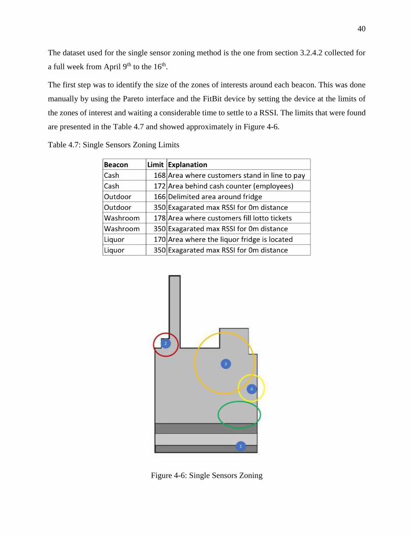
40

The dataset used for the single sensor zoning method is the one from section 3.2.4.2 collected for

a full week from April 9th to the 16th.

The first step was to identify the size of the zones of interests around each beacon. This was done

manually by using the Pareto interface and the FitBit device by setting the device at the limits of

the zones of interest and waiting a considerable time to settle to a RSSI. The limits that were found

are presented in the Table 4.7 and showed approximately in Figure 4-6.

Table 4.7: Single Sensors Zoning Limits

Figure 4-6: Single Sensors Zoning

41

In Figure 4-6, the green circle is the zone captured by beacon #1 which corresponds to the cash

area, the red circle is the zone captured by beacon #2 which corresponds to the washroom area, the

orange circle is captured by beacon #3 which corresponds to the liquor area and the yellow circle

is captured by beacon #4, which corresponds to the outdoor area.

The next step was to separate the raw data into each day of the week. The timestamp was given in

Unix epoch format which is the number of milliseconds since Jan 1, 1970. To separate the data, an

online converter was used to identify the limits of each day of the week. For example, Monday

April 9th 2018 12:00:00 AM is 1523246400000 in Unix epoch.

After separating in days, some data pre-processing had to be performed on the raw CSV values.

First we removed all beacon captures as Bluetooth devices from the collection. This was done by

removing from the python dataframe all entries where the “DeviceTags” was described as a beacon

of any kind. Then other irrelevant devices were removed from the collection such as Bluetooth

coming from objects being transported in cars such as an Apple TV, a camera, or any other non-

wearable or smartphone device. This was also done by filtering the “DeviceTags”. Finally, the last

cleanup was done by removing employee or store Bluetooth devices data from the collection. This

was done by checking the amount of time a certain Bluetooth device ID was captured. On average,

most captures were collected between 1 to 40 times. Then there was a discrepancy were a few were

captured over 1000 times. Having removed device IDs which appeared a significant amount of

times more than the majority of captures being captured 1 to 40 times, we can say with high

confidence that employee devices have been removed in this pre-processing step. These

discrepancies were removed from the data collection to obtain only customer data.

Finally, the code was run to identify the number of unique Bluetooth devices presences, hence

unique customers, per beacon per day. The returned output is summarized in Table 4.8.

42

Table 4.8: Number of Presences Per Beacon

The next step involves finding a scale to separate the data into quiet, normal and busy for the data

analysis portion. The logic used to separate the data is shown in Table 4.9. The value of a “range”

corresponds to the maximum value minus the minimum value. Values lesser than “average –

range/count” are considered as quiet and values greater than “average + range/count” are

considered busy. The colour formatting shown in Table 4.9 is applied on all beacons and sales data

tables (section 4.2) to visually show the classification.

Table 4.9: Classification Logic for Sales Proportions and Beacon Activity

In Table 4.10, Table 4.11 and Table 4.12, proportions are presented to discuss potential insights

that can be extracted from this data. Table 4.10 shows the absolute activity proportions for each

given day, Table 4.11 shows the activity proportions for each given beacon for all days and Table

4.12 shows the relative activity all beacons for each given day. The relative activity was found by

comparing each beacon activity per day with the average of the whole week. For example, on

Monday the cash relative proportion is calculated as such: 46/(average of the week) = 18%. Thick

lines were added to the tables to visually clarify when the rows or columns are being compared for

proportions.

43

Table 4.10: Presence at Beacons (Per Day Proportions)

Table 4.11: Presence at Beacons (Per Beacon Proportions)

Table 4.12: Presence at Beacons (Per Day Relative Proportions)

From Table 4.10, some information can be extracted. We can observe that the cash is always the

busiest area among the 3 zones, which would be the expected result from a gas station convenience

store. To clarify that the cashier is not part of the count, looking back at Figure 4-6, the cashier

44

stands behind the counter and the zone delimited by RSSI signal does not include the cashier

position hence the data contains only customers waiting at the cash. This also does confirm a certain

level of accuracy in the data extracted as the cash beacon is what would be expected as the busiest

one at all days. Another interesting information that can be extracted is the consistent higher

proportions of presence at the “Outdoor” zone (which consists of mostly cold non-alcoholic drinks)

versus the “Washroom” (Lottery) and “Liquor” zones. This can lead to interesting applications for

the store manager such as displaying promotions in that area knowing that customer traffic is

higher. In section 4.2 we will go more in depth into comparing these results with the sales reports

for that same week using a decision tree to validate further the accuracy of the results from the

beacons. Table 4.11 is showing more varying data when looking at the activity for a beacon

throughout the whole week. It is harder to extract useful information by simple analysing it

visually. Table 4.12 can also potentially show us useful information, where relative activity is

compared. Also with a visual inspection it is harder to analyze, and same as Table 4.11, it will be

explored more in details in section 4.2.

Comparing with the results from the four-sensor triangulation method, the data is more reliable

when using a single sensor for general positioning information on customer activity. This is

because in section 4.1.2 we bypass the issue of precision by not looking at a precise pathway but

simply a presence or not of a device within the zone.

4.2 Sales & Beacons Data Analysis

In this section, we will be attempting to perform a data analysis on the sales data in correlation with

the single sensor zoning data collected from the previous section 4.1.2. The purpose is to prove

that there is a correlation between customer’s physical activities within the store and the sales

generated. This correlation will show that the data collected from an IoT system can be used to

study and improve store sales. For the sales data, we were given access by the convenience store

to all the cash register history for the given week of data collection from section 3.3.1.2. The

categories chosen to be included in the analysis are all products that can be found around the studied

beacons. Non-alcoholic drinks are found around the outdoor beacon, sweets and tobacco products

are found around the cash beacon, alcoholic drinks and salty snacks are found around the liquor

beacon. For confidentiality reasons, the raw sales data cannot be attached to this research project,

but proportions will be shown. In Table 4.13, the sales proportions of each category calculated was

45

taken relative to the whole week (for example, on Monday 11.6% of the weekly non-alcoholic

drinks were made).

Table 4.13: Sales Proportions Per Category (For the Week)

With the classification logic that was explained in Table 4.9, two different proportions were

compared for the sales data. The first comparison, found in Table 4.14, shows the sales proportions

for each category over a week. The second comparison is done in Table 4.15, where it shows the

sales proportions of each day over all categories. The colour coding and logic is the same as shown

in Table 4.9.

Table 4.14: Sales Proportions Relative to The Week

Table 4.15: Sales Proportions Relative to The Categories

46

We then proceed to using a decision tree data mining method to demonstrate the potential utilities

of an IoT system to a brick and mortar retail environment. The decision tree algorithm used is

presented in section 3.4.

For this experimentation, four different datasets were used. The used data involved the activity of

each beacon from section 4.1.2 combined with the sales proportions from this section. The first

dataset consists of Table 4.11 and Table 4.14, the second dataset consists of Table 4.11 and Table

4.15, the third dataset consists of Table 4.12 and Table 4.14 and finally the fourth dataset consists

of Table 4.12 and Table 4.15. These table combinations consist of different combos of activity

comparisons that are either spread over a week or over all beacons as previously discussed. This is

done to find the most accurate combination per the decision tree algorithm. Datasets can be seen

in Table 4.16 to Table 4.19.

Table 4.16: Dataset 1 Using Table 4.11 and Table 4.14

Table 4.17: Dataset 2 Using Table 4.11 And Table 4.15

Table 4.18: Dataset 3 Using Table 4.12 Table 4.14

47

Table 4.19: Dataset 4 Using Table 4.12 Table 4.15

Each one of the four datasets were then loaded in individual python scripts. The structure of each

script is the same. The first step within the script was to define which variables are used as predictor

variables and which ones as outcome variables. Days and beacon activity were chosen for this

study as our predictor variable and each sales category individually as our outcome variable. The

second step is to define the training size and the test size for the decision tree. It was chosen that

the test size sample would be 25% and the training size sample would be 75% of the dataset. The

third step consists of applying the CART algorithm with the pre-compiled method and exporting it

visually to PDF files to create visual decision trees. The last step involves applying the created

decision tree on each category and evaluating its accuracy. The accuracy of each dataset and each

category is shown in Table 4.20 to Table 4.22. Accuracy is simply calculated by the python script

by computing how many real predictions are done over the total testing sample. The complete

python script can be found in appendix C with a sample output for dataset 1.

Table 4.20: Dataset 1 Prediction Accuracy

48

Table 4.21: Dataset 2 Prediction Accuracy

Table 4.22: Dataset 3 Prediction Accuracy

Table 4.23: Dataset 4 Prediction Accuracy

Analyzing the accuracy results, we can see that there is potential for a correlation between the

customer’s physical locations within the store and sales data. This section will examine more

closely the decision tree in Figure 4-7 that was formed from dataset 4, shown in a classified form

in Table 4.25, and using alcoholic drinks as the outcome variables. All decision trees produced

can be found in appendix E.

49

Table 4.24 shows a legend of the values used in the decision trees. The python script works better

with numbers so the days of the week and the activity classification terms were transformed into

integers.

Table 4.24: Decision Tree Legend

Table 4.25: Dataset 4 Classified Values

50

Figure 4-7: Alcoholic Drinks from Dataset 4 Decision Tree

This decision tree was chosen to be examined more closely because it returned a 100% accuracy

when tested in the python script. The colour coding is done automatically by the python script and

is not relevant for any analysis. The decision tree will be examined closely in the next paragraph.

While looking at the results of this decision tree, it is important to keep in mind that this research

is done on an exploratory basis, hence the amount of data collected represents an idea of what a

lengthy implementation could lead to. For this research, we have a week of data collection which

means that our total sample size is 7, which includes a training sample size of 5 and a test sample

size of 2.

Analyzing the decision tree, first thing is to clarify what each line represents. The first line, which

contains possible values of X[1] to X[5], represents the column where an attribute is observed. By

cross-referencing with Table 4.25, X[1] represents the day column, X[2] represents the cash beacon

column, X[3] represents the outdoor beacon column, X[4] represents the washroom beacon column

and X[5] represents the liquor beacon column. As for the value of the attribute, by cross referencing

with

Table 4.24, 1 means quiet, 2 means normal and 3 means busy. On the next line of the decision tree,

we find the Gini impurity value. As previously discussed, a lower value is optimal meaning that

the separation puts most of the samples in the same class. In the case of this decision trees, the

51

similarities are based on sales activity being quiet, normal or busy. On the next line, the sample

size represents the number of samples that are on the node. Finally, on the last line, the value with

the three numbers represent the outcome of the output variable on that node where the first number

is the number of outcomes with quiet, the second number is the number of outcomes with normal

and the last number is the number of outcomes with busy.

If we follow the path with the circle label 1, it means that if the washroom beacon is not quiet

(relative to the week), the outdoor beacon is quiet and the cash beacon is busy, then the expected

alcoholic drinks sales should be quiet (relative to other categories).

These findings are interesting and show that the customer’s behaviors have a correlation with the

store sales. A store manager could extract practical applications out of this decision tree. First we

will clarify which products can be found at the mentioned beacons by cross-referencing with

Table 3.1 and Figure 4-6 for the single sensor zoning limits. At the washroom beacon, the products

within that zone are lottery tickets, for the outdoor beacon we can find cold non-alcoholic drinks

and at the cash beacon we find the cash register lineup as well as gum, sweets and tobacco products.

This would mean that by looking at outcome of point 1 pathway, if for that day there is low activity

at both lottery tickets and cold non-alcoholic drinks, but while having a busy cash lineup, then the

store manager can also expect low alcoholic drink sales. An example of a practical marketing

application could be as such; an automatic alert is set up to trigger on the manager’s smart phone

when the conditions of decision tree pathway 1 are satisfied. This alert could recommend setting

up special promotions for the rest of the day on alcoholic products to boost sales if inventory needs

to be cleared on that day or week.

Such decision trees can also help store owners better understand when some products are expected

to sell more, which can lead to operational decisions such as showcasing new products during the

times and zones when and where sales are expected to be higher. Those are just some applications

amongst others that can come out of an IoT system.

52

CHAPTER 5 CONCLUSION

This research was meant to demonstrate, from a first experimental IoT system setup in a traditional

retail store, that data analytics methods can be applied to extract useful information and insights to

improve store operations. The applications of most interest did not come from tracing precise paths

coming from the Bluetooth devices but became more useful when the IoT system was observed

from a less granular point of view. This led to showcase more practical possibilities to exploit the

data with data mining methods. From less precise information, more useful applications came out

of it such as smart alerts when a certain pattern is detected from the IoT system. This same

information can also potentially help understand business owners the behavior of their sales when

it comes to products, days or zones of interest within the store.

After performing a collection from the Bluetooth beacons and applying a first data analysis which

traces each unique customer’s pathway inside the store, we encountered the first limitation to the

system, which is the Bluetooth precision. Due to this limitation, our findings were that a precise

pathway could not be traced with the current setup put in place and by using the linear or

logarithmic correlation methods. However, readings based on single sensors provided much more

reliable results which were used for the sales data analysis. In the recommendations below we

discuss what should be done instead to receive data with better granularity in future work.

The second demonstration of this research project was to show a correlation between more general

positional data, which in our case was the activity proportions at different beacons, and the sales

numbers classified per categories. We have indeed showed, in an exploratory basis, that it is

possible to find correlations between BLE-sensed customer activity and sales activities, by

applying a decision tree CART method, which could be used to predict the sales of different

categories of items depending on the activity at different zones.

Recommendations for further experimentations would be to include an integrated Bluetooth and

WIFI IoT system instead to increase locational precision from customer’s smart devices; in that

case, a more careful attention would be required to the ethical and social issues that the research

may arise, especially if a field data collection with real customers is attempted. Another

recommendation would be to perform these experimentations in a larger zone, preferably spanning

over multiple floors as that is when the sensor technology will work best. Finally, we also

53

recommend to perform the data collection over multiple weeks and applying decision tree

algorithms now that we know from this pilot project of its potential.

54

BIBLIOGRAPHY

Ashton, K. (2009). That ‘internet of things’ thing. RFID journal, 22(7), 97-114.

Atzori, L., Iera, A., & Morabito, G. (2010). The Internet of Things: A survey. Computer Networks,

54(15), 2787-2805. doi:10.1016/j.comnet.2010.05.010

Banafa, A. (2016). IoT Standardization and Implementation Challenges. IEEE Internet of Things.

Bandyopadhyay, D., & Sen, J. (2011). Internet of things: Applications and challenges in technology

and standardization. Wireless Personal Communications, 58(1), 49-69.

Brownlee, J. (2016). Supervised and Unsupervised Machine Learning Algorithms. Retrieved from

https://machinelearningmastery.com/supervised-and-unsupervised-machine-learning-

algorithms/

Chawathe, S. S. (2008). Beacon placement for indoor localization using bluetooth. Paper presented

at the Intelligent Transportation Systems, 2008. ITSC 2008. 11th International IEEE

Conference on.

Columbus, L. (2017). Internet Of Things Will Revolutionize Retail. Retrieved from

https://www.forbes.com/sites/louiscolumbus/2017/03/19/internet-of-things-will-

revolutionize-retail/ - 56d24b785e58

Cunche, M. (2014). I know your MAC Address: Targeted tracking of individual using Wi-Fi.

Journal of Computer Virology and Hacking Techniques, 10(4), 219-227.

Cunche, M., Kaafar, M.-A., & Boreli, R. (2014). Linking wireless devices using information

contained in Wi-Fi probe requests. Pervasive and Mobile Computing, 11, 56-69.

Fagerstrøm, A., Eriksson, N., & Sigurðsson, V. (2017). What’s the “Thing” in Internet of Things

in Grocery Shopping? A Customer Approach. Procedia Computer Science, 121, 384-388.

Ferro, E., & Potorti, F. (2005). Bluetooth and Wi-Fi wireless protocols: a survey and a comparison.

IEEE Wireless Communications, 12(1), 12-26.

Gomez, C., Oller, J., & Paradells, J. (2012). Overview and evaluation of bluetooth low energy: An

emerging low-power wireless technology. Sensors, 12(9), 11734-11753.

Gregory, J. (2014). The Internet of Things: Revolutionizing the Retail Industry. Accenture

Strategy.

Gubbi, J., Buyya, R., Marusic, S., & Palaniswami, M. (2013). Internet of Things (IoT): A vision,

architectural elements, and future directions. Future generation computer systems, 29(7),

1645-1660.

Hagberg, J., Jonsson, A., & Egels-Zandén, N. (2017). Retail digitalization: Implications for

physical stores. Journal of Retailing and Consumer Services.

Hwang, I., & Jang, Y. J. (2017). Process Mining to Discover Shoppers' Pathways at a Fashion

Retail Store Using a WiFi-Base Indoor Positioning System. Ieee Transactions on

Automation Science and Engineering, 14(4), 1786-1792. doi:10.1109/tase.2017.2692961

ISO. (2018). Internet of Things Reference Architecture (IoT RA). In ISO/IEC CD 30141.

55

Kesavaraj, G., & Sukumaran, S. (2013). A study on classification techniques in data mining. Paper

presented at the Computing, Communications and Networking Technologies (ICCCNT),

2013 Fourth International Conference on.

Kortuem, G., Kawsar, F., Fitton, D., & Sundramoorthy, V. (2010). Smart Objects as Building

Blocks for the Internet of Things. Ieee Internet Computing, 14(1), 44-51.

doi:10.1109/mic.2009.143

Kriz, P., Maly, F., & Kozel, T. (2016). Improving indoor localization using bluetooth low energy

beacons. Mobile Information Systems, 2016.

Lee, I., & Lee, K. (2015). The Internet of Things (IoT): Applications, investments, and challenges

for enterprises. Business Horizons, 58(4), 431-440.

Li, L., Xiaoguang, H., Ke, C., & Ketai, H. (2011). The applications of wifi-based wireless sensor

network in internet of things and smart grid. Paper presented at the Industrial Electronics

and Applications (ICIEA), 2011 6th IEEE Conference on.

Longo, S., Kovacs, E., Franke, J., & Martin, M. (2013). Enriching shopping experiences with

pervasive displays and smart things. Paper presented at the Proceedings of the 2013 ACM

conference on Pervasive and ubiquitous computing adjunct publication.

Manyika, J., Chui, M., Bisson, P., Woetzel, J., Dobbs, R., Bughin, J., & Aharon, D. (2015). The

Internet of Things: Mapping the Value Beyond the Hype. McKinsey Global Institute.

Moro, S., Laureano, R., & Cortez, P. (2011). Using data mining for bank direct marketing: An

application of the crisp-dm methodology. Paper presented at the Proceedings of European

Simulation and Modelling Conference-ESM'2011.

Palumbo, F., Barsocchi, P., Chessa, S., & Augusto, J. C. (2015). A stigmergic approach to indoor

localization using bluetooth low energy beacons. Paper presented at the Advanced Video

and Signal Based Surveillance (AVSS), 2015 12th IEEE International Conference on.

Perera, C., Zaslavsky, A., Christen, P., & Georgakopoulos, D. (2014). Context aware computing

for the internet of things: A survey. IEEE communications surveys & tutorials, 16(1), 414-

454.

Radhakrishnan, B., Shineraj, G., & Anver Muhammed, K. (2013). Application of Data Mining In

Marketing. IJCSN International Journal of Computer Science and Network, ISSN (Online),

2277-5420.

Rutkowski, L., Jaworski, M., Pietruczuk, L., & Duda, P. (2014). The CART decision tree for

mining data streams. Information Sciences, 266, 1-15.

Saloni, S., & Hegde, A. (2016). WiFi-aware as a connectivity solution for IoT pairing IoT with

WiFi aware technology: Enabling new proximity based services. Paper presented at the

Internet of Things and Applications (IOTA), International Conference on.

Scikit-learn. (2018). DecisionTreeClassifier. Retrieved from http://scikit-

learn.org/stable/modules/generated/sklearn.tree.DecisionTreeClassifier.html

Shah, S. H., & Yaqoob, I. (2016). A survey: Internet of Things (IOT) technologies, applications

and challenges. Paper presented at the Smart Energy Grid Engineering (SEGE), 2016 IEEE.

56

Singh, S., & Gupta, P. (2014). Comparative study ID3, cart and C4. 5 decision tree algorithm: a

survey. International Journal of Advanced Information Science and Technology (IJAIST),

27(27), 97-103.

Zhuang, Y., Yang, J., Li, Y., Qi, L., & El-Sheimy, N. (2016). Smartphone-based indoor localization

with bluetooth low energy beacons. Sensors, 16(5), 596.

57

APPENDIX A – PARETO DATA COLLECTION CODES

Non matrix Pareto data collection code

58

Matrix Pareto data collection code

59

APPENDIX B – RAW DATA

Non-Matrix Form Raw Data Excerpt

60

Matrix Form Raw Data Excerpt

61

Fitbit Validation Raw Data Excerpt & Defined Zone Using Linear Function

62

Fitbit Validation Raw Data Excerpt & Defined Zone Using Log Function

63

APPENDIX C – PYTHON CODES

Pathway Tracing Code

import pandas as pd

#-----------------------------------------------------------------------------#

# Data Loading #

#-----------------------------------------------------------------------------#

data_dir = '/Data_Collection/April_29/'

linear_data_file = 'eventlog-180429123943.csv'

log_data_file = 'eventlog-180429123943_log.csv'

linear_df = pd.read_csv(data_dir + linear_data_file,

dtype={"time" : long,

"event" : str,

"sessionId" : str,

"sessionDuration" : float,

"deviceId" : str,

"deviceTags" : str,

"receiverId" : str,

"receiverTags" : str,

"receiverDirectory": str,

"receiverUrl": str,

"position" : str,

"isPerson" : str,

"cash" : int,

"outdoor" : int,

"washroom" : int,

"liquor" : int,

"Zone" : int})

log_df = pd.read_csv(data_dir + log_data_file,

dtype={"time" : long,

"event" : str,

"sessionId" : str,

"sessionDuration" : float,

"deviceId" : str,

"deviceTags" : str,

"receiverId" : str,

"receiverTags" : str,

"receiverDirectory": str,

"receiverUrl": str,

"position" : str,

"isPerson" : str,

64

"cash" : int,

"outdoor" : int,

"washroom" : int,

"liquor" : int,

"Zone" : int})

#-----------------------------------------------------------------------------#

# Linear Data Pre-Processing #

#-----------------------------------------------------------------------------#

# Add new column:

# Purpose: Identifying fitbit testing device

# Query: Fitbit testing device, Device ID: 7802b7225f58

deviceID = '7802b7225f58'

isTestingDevice = []

for row in linear_df['deviceId']:

if deviceID in row:

isTestingDevice.append(True)

else:

isTestingDevice.append(False)

linear_df['isTestingDevice'] = isTestingDevice

# Create new dataframe

# Content: Data points containing only testing device

linear_testing_device_df = linear_df.query('isTestingDevice == True')

#-----------------------------------------------------------------------------#

# Log Data Pre-Processing #

#-----------------------------------------------------------------------------#

# Add new column:

# Purpose: Identifying fitbit testing device

# Query: Fitbit testing device, Device ID: 7802b7225f58

deviceID = '7802b7225f58'

isTestingDevice = []

for row in log_df['deviceId']:

if deviceID in row:

isTestingDevice.append(True)

else:

65

isTestingDevice.append(False)

log_df['isTestingDevice'] = isTestingDevice

# Create new dataframe

# Content: Data points containing only testing device

log_testing_device_df = log_df.query('isTestingDevice == True')

#-----------------------------------------------------------------------------#

# Linear Result validations #

#-----------------------------------------------------------------------------#

# Dataframe where all points gathered are not outside (zone 13)

linear_inside_df = linear_testing_device_df.query('Zone != 13')

# Zones during complete testing time: 12:39:00 PM to 12:52:00 PM

print('Linear complete testing time')

print(linear_inside_df.query('time >= 1525019940000 & time <= 1525020720000'))

# Actual Zones Pathway: 1(4)->4->7->10->12->10->8->11->9->6->3->1

# Returned Zones Pathway: 4->7->4->5->6->5->2

#-----------------------------------------------------------------------------#

# Log Result validations #

#-----------------------------------------------------------------------------#

# Dataframe where all points gathered are not outside (zone 13)

log_inside_df = log_testing_device_df.query('Zone != 13')

# Zones during complete testing time: 12:39:00 PM to 12:52:00 PM

print('Log complete testing time')

print(log_inside_df.query('time >= 1525019940000 & time <= 1525020720000'))

# Actual Zones Pathway: 1(4)->4->7->10->12->10->8->11->9->6->3->1

# Returned Zones Pathway: 9

Pathway Tracing Code Output

Linear complete testing time

time event sessionId \

25 1525019993512 displacement 7265656c-0000-4000-8048-7802b7225f58

36 1525019999905 keep-alive 7265656c-0000-4000-8048-7802b7225f58

487 1525020222802 displacement 7265656c-0000-4000-8048-7802b7225f58

502 1525020228639 keep-alive 7265656c-0000-4000-8048-7802b7225f58

521 1525020237746 displacement 7265656c-0000-4000-8048-7802b7225f58

538 1525020243731 keep-alive 7265656c-0000-4000-8048-7802b7225f58

599 1525020272832 keep-alive 7265656c-0000-4000-8048-7802b7225f58

66

611 1525020278652 keep-alive 7265656c-0000-4000-8048-7802b7225f58

637 1525020290500 keep-alive 7265656c-0000-4000-8048-7802b7225f58

651 1525020296934 keep-alive 7265656c-0000-4000-8048-7802b7225f58

660 1525020302619 keep-alive 7265656c-0000-4000-8048-7802b7225f58

671 1525020308603 keep-alive 7265656c-0000-4000-8048-7802b7225f58

686 1525020316521 displacement 7265656c-0000-4000-8048-7802b7225f58

720 1525020332683 keep-alive 7265656c-0000-4000-8048-7802b7225f58

752 1525020349570 keep-alive 7265656c-0000-4000-8048-7802b7225f58

761 1525020354935 keep-alive 7265656c-0000-4000-8048-7802b7225f58

783 1525020365676 keep-alive 7265656c-0000-4000-8048-7802b7225f58

948 1525020447640 keep-alive 7265656c-0000-4000-8048-7802b7225f58

959 1525020453514 keep-alive 7265656c-0000-4000-8048-7802b7225f58

969 1525020459625 keep-alive 7265656c-0000-4000-8048-7802b7225f58

975 1525020465546 keep-alive 7265656c-0000-4000-8048-7802b7225f58

1018 1525020491887 displacement 7265656c-0000-4000-8048-7802b7225f58

1026 1525020497650 keep-alive 7265656c-0000-4000-8048-7802b7225f58

1079 1525020526551 keep-alive 7265656c-0000-4000-8048-7802b7225f58

1090 1525020532134 keep-alive 7265656c-0000-4000-8048-7802b7225f58

1150 1525020562735 displacement 7265656c-0000-4000-8048-7802b7225f58

1270 1525020627823 keep-alive 7265656c-0000-4000-8048-7802b7225f58

1386 1525020690022 keep-alive 7265656c-0000-4000-8048-7802b7225f58

sessionDuration deviceId deviceTags receiverId receiverTags \

25 176470.0 7802b7225f58 NaN 001bc50940820014 Owl-in-one

36 182661.0 7802b7225f58 NaN 001bc50940820014 Owl-in-one

487 405560.0 7802b7225f58 NaN 001bc50940820014 Owl-in-one

502 411735.0 7802b7225f58 NaN 001bc50940820014 Owl-in-one

521 420512.0 7802b7225f58 NaN 001bc50940820014 Owl-in-one

538 426537.0 7802b7225f58 NaN 001bc50940820014 Owl-in-one

599 455590.0 7802b7225f58 NaN 001bc50940820014 Owl-in-one

611 462008.0 7802b7225f58 NaN 001bc50940820014 Owl-in-one

637 473287.0 7802b7225f58 NaN 001bc50940820014 Owl-in-one

651 479686.0 7802b7225f58 NaN 001bc50940820014 Owl-in-one

660 485397.0 7802b7225f58 NaN 001bc50940820014 Owl-in-one

671 491448.0 7802b7225f58 NaN 001bc50940820014 Owl-in-one

686 499314.0 7802b7225f58 NaN 001bc50940820015 Owl-in-one

720 515510.0 7802b7225f58 NaN 001bc50940820015 Owl-in-one

752 532596.0 7802b7225f58 NaN 001bc50940820015 Owl-in-one

761 537694.0 7802b7225f58 NaN 001bc50940820015 Owl-in-one

783 548617.0 7802b7225f58 NaN 001bc50940820015 Owl-in-one

948 630796.0 7802b7225f58 NaN 001bc50940820015 Owl-in-one

959 636425.0 7802b7225f58 NaN 001bc50940820015 Owl-in-one

969 642586.0 7802b7225f58 NaN 001bc50940820015 Owl-in-one

975 648590.0 7802b7225f58 NaN 001bc50940820015 Owl-in-one

1018 674679.0 7802b7225f58 NaN 001bc50940820015 Owl-in-one

1026 680646.0 7802b7225f58 NaN 001bc50940820015 Owl-in-one

1079 709520.0 7802b7225f58 NaN 001bc50940820011 Owl-in-one

67

1090 714885.0 7802b7225f58 NaN 001bc50940820011 Owl-in-one

1150 745486.0 7802b7225f58 NaN 001bc50940820011 Owl-in-one

1270 810578.0 7802b7225f58 NaN 001bc50940820011 Owl-in-one

1386 872773.0 7802b7225f58 NaN 001bc50940820011 Owl-in-one

receiverDirectory receiverUrl position \

25 poly:12339:Toilettes-Lait undefined -73.729433 | 45.603054

36 poly:12339:Caisse undefined -73.729215 | 45.603003

487 poly:12339:Toilettes-Lait undefined -73.729433 | 45.603054

502 poly:12339:Bieres-Tablettes undefined -73.729383 | 45.603081

521 poly:12339:Toilettes-Lait undefined -73.729433 | 45.603054

538 poly:12339:Toilettes-Lait undefined -73.729433 | 45.603054

599 poly:12339:Toilettes-Lait undefined -73.729433 | 45.603054

611 poly:12339:Bieres-Tablettes undefined -73.729383 | 45.603081

637 poly:12339:Caisse undefined -73.729215 | 45.603003

651 poly:12339:Toilettes-Lait undefined -73.729433 | 45.603054

660 poly:12339:Outdoor undefined -73.729287 | 45.60309

671 poly:12339:Caisse undefined -73.729215 | 45.603003

686 poly:12339:Toilettes-Lait undefined -73.729433 | 45.603054

720 poly:12339:Outdoor undefined -73.729287 | 45.60309

752 poly:12339:Outdoor undefined -73.729287 | 45.60309

761 poly:12339:Bieres-Tablettes undefined -73.729383 | 45.603081

783 poly:12339:Toilettes-Lait undefined -73.729433 | 45.603054

948 poly:12339:Caisse undefined -73.729215 | 45.603003

959 poly:12339:Toilettes-Lait undefined -73.729433 | 45.603054

969 poly:12339:Outdoor undefined -73.729287 | 45.60309

975 poly:12339:Toilettes-Lait undefined -73.729433 | 45.603054

1018 poly:12339:Bieres-Tablettes undefined -73.729383 | 45.603081

1026 poly:12339:Toilettes-Lait undefined -73.729433 | 45.603054

1079 poly:12339:Bieres-Tablettes undefined -73.729383 | 45.603081

1090 poly:12339:Outdoor undefined -73.729287 | 45.60309

1150 poly:12339:Outdoor undefined -73.729287 | 45.60309

1270 poly:12339:Toilettes-Lait undefined -73.729433 | 45.603054

1386 poly:12339:Outdoor undefined -73.729287 | 45.60309

isPerson cash outdoor washroom liquor Zone isTestingDevice

25 unlikely 158 147 163 161 4 True

36 unlikely 159 150 163 159 4 True

487 unlikely 151 151 172 164 7 True

502 unlikely 153 152 172 164 7 True

521 unlikely 152 150 173 164 7 True

538 unlikely 152 149 173 164 7 True

599 unlikely 152 150 173 164 7 True

611 unlikely 152 150 173 164 7 True

637 unlikely 153 150 173 164 7 True

651 unlikely 153 150 172 164 7 True

660 unlikely 153 149 172 163 7 True

68

671 unlikely 152 149 166 157 4 True

686 unlikely 154 145 163 165 4 True

720 unlikely 160 166 164 168 5 True

752 unlikely 160 166 164 168 5 True

761 unlikely 161 166 164 168 5 True

783 unlikely 160 166 164 169 5 True

948 unlikely 158 161 159 165 5 True

959 unlikely 160 161 163 170 5 True

969 unlikely 162 162 163 171 5 True

975 unlikely 161 161 164 170 5 True

1018 unlikely 162 163 164 170 5 True

1026 unlikely 160 163 160 170 5 True

1079 unlikely 166 163 155 164 6 True

1090 unlikely 166 164 155 164 6 True

1150 unlikely 165 164 158 164 5 True

1270 unlikely 167 155 156 157 2 True

1386 unlikely 170 146 154 154 2 True

Log complete testing time

time event sessionId \

1128 1525020000000 keep-alive 7265656c-0000-4000-8048-7802b7225f58

sessionDuration deviceId deviceTags receiverId receiverTags \

1128 734567.0 7802b7225f58 NaN 001bc50940820012 Owl-in-one

receiverDirectory receiverUrl position isPerson cash \

1128 poly:12339:Outdoor undefined -73.729287 | 45.60309 unlikely 158

outdoor washroom liquor Zone isTestingDevice

1128 165 146 162 9 True

69

Single Sensor Zoning Code

import pandas as pd

import numpy as np

#-----------------------------------------------------------------------------#

# Data Loading #

#-----------------------------------------------------------------------------#

data_dir = '/Users/Georges/Google Drive/Education/ResearchProject/Store/Collection/'

data_file = 'eventlog-180409203116.csv'

df = pd.read_csv(data_dir + data_file,

dtype={"time" : long,

"event" : str,

"sessionId" : str,

"sessionDuration" : float,

"deviceId" : str,

"deviceTags" : str,

"receiverId" : str,

"receiverTags" : str,

"receiverDirectory": str,

"receiverUrl": str,

"position" : str,

"isPerson" : str,

"cash" : int,

"outdoor" : int,

"washroom" : int,

"liquor" : int,

"Zone" : int})

#-----------------------------------------------------------------------------#

# Limit Definition #

#-----------------------------------------------------------------------------#

# Delimited zones found during testing on May 13th

cashLowerLimit = 168 # Area where customers stand in line to pay

cashHigherLimit = 172 # Area behind cash counter (employees)

outdoorLowerLimit = 166 # Delimited area around fridge

outdoorHigherLimit = 350 # Exagarated max RSSI for 0m distance

washroomLowerLimit = 178 # Area where customers fill lotto tickets

washroomHigherLimit = 350 # Exagarated max RSSI for 0m distance

liquorLowerLimit = 170 # Area where the liqor fridge is located

liquorHigherLimit = 350 # Exagarated max RSSI for 0m distance

# Day delimitation for a 1 week sample (April 9-16, 2018)

'''

70

Online epoch to human date converter used

Source: https://www.epochconverter.com/

'''

firstMondayLowerLimit = 1523246400000

firstMondayUpperLimit = 1523332799000

secondMondayLowerLimit = 1523851200000

secondMondayUpperLimit = 1523937599000

tuesdayLowerLimit = 1523332800000

tuesdayUpperLimit = 1523419199000

wednesdayLowerLimit = 1523419200000

wednesdayUpperLimit = 1523505599000

thursdayLowerLimit = 1523505600000

thursdayUpperLimit = 1523591999000

fridayLowerLimit = 1523592000000

fridayUpperLimit = 1523678399000

saturdayLowerLimit = 1523678400000

saturdayUpperLimit = 1523764799000

sundayLowerLimit = 1523764800000

sundayUpperLimit = 1523851199000

#-----------------------------------------------------------------------------#

# Data Pre-Processing #

#-----------------------------------------------------------------------------#

# Remove beacon data from collection

df.query("deviceTags != 'beacon | indoorpositioning' ", inplace=True)

df.query("deviceTags != 'beacon' ", inplace=True)

df.query("deviceTags != 'track | beacon' ", inplace=True)

df.query("deviceTags != 'iBeacon' ", inplace=True)

# Remove irrelevant devices from collection using device tags

# Removed device tags: AppleTV, smarthome, camera

df.query("deviceTags != 'AppleTV' ", inplace=True)

df.query("deviceTags != 'smarthome' ", inplace=True)

df.query("deviceTags != 'camera' ", inplace=True)

# Remove device ID's that appear over 1000 times in the dataframe

# These devices skew the data and could be employees cell phones

# or other bluetooth devices installed inside the store.

# Method used to identify devices: df.deviceId.value_counts()

# Removed device IDs: ac233fa00341, 2091484bb4ce, 2091484bb3fe,

# 2091484bb4bf, 2091484bb4c7, 2c41a12608f4,

# 883d240b4861

df.query("deviceId != 'ac233fa00341' ", inplace=True)

df.query("deviceId != '2091484bb4ce' ", inplace=True)

df.query("deviceId != '2091484bb3fe' ", inplace=True)

df.query("deviceId != '2091484bb4bf' ", inplace=True)

71

df.query("deviceId != '2091484bb4c7' ", inplace=True)

df.query("deviceId != '2c41a12608f4' ", inplace=True)

df.query("deviceId != '883d240b4861' ", inplace=True)

# Detect presence in defined beacon zones

presenceAtCash = []

presenceAtOutdoor = []

presenceAtWashroom = []

presenceAtLiquor = []

for row in df['cash']:

if row > cashLowerLimit and row < cashHigherLimit:

presenceAtCash.append(True)

else:

presenceAtCash.append(False)

for row in df['outdoor']:

if row > cashLowerLimit and row < cashHigherLimit:

presenceAtOutdoor.append(True)

else:

presenceAtOutdoor.append(False)

for row in df['washroom']:

if row > cashLowerLimit and row < cashHigherLimit:

presenceAtWashroom.append(True)

else:

presenceAtWashroom.append(False)

for row in df['liquor']:

if row > cashLowerLimit and row < cashHigherLimit:

presenceAtLiquor.append(True)

else:

presenceAtLiquor.append(False)

df['presenceAtCash'] = presenceAtCash

df['presenceAtOutdoor'] = presenceAtOutdoor

df['presenceAtWashroom'] = presenceAtWashroom

df['presenceAtLiquor'] = presenceAtLiquor

# Remove data with no presence at any beacon

df.query('presenceAtCash == True or \

presenceAtOutdoor == True or \

presenceAtWashroom == True or \

presenceAtLiquor == True', inplace=True)

# Create new days column

day = []

72

for row in df['time']:

if (row > firstMondayLowerLimit and row < firstMondayUpperLimit) \

or (row > secondMondayLowerLimit and row < secondMondayUpperLimit):

day.append('Monday')

elif row > tuesdayLowerLimit and row < tuesdayUpperLimit:

day.append('Tuesday')

elif row > wednesdayLowerLimit and row < wednesdayUpperLimit:

day.append('Wednesday')

elif row > thursdayLowerLimit and row < thursdayUpperLimit:

day.append('Thursday')

elif row > fridayLowerLimit and row < fridayUpperLimit:

day.append('Friday')

elif row > saturdayLowerLimit and row < saturdayUpperLimit:

day.append('Saturday')

elif row > sundayLowerLimit and row < sundayUpperLimit:

day.append('Sunday')

df['day'] = day

#-----------------------------------------------------------------------------#

# Data Analysis #

#-----------------------------------------------------------------------------#

# Traffic per day, per beacon zone

# Printed values shown below

print('Monday: ')

print('cash: ')

print(df.query("day == 'Monday' and presenceAtCash == True").deviceId.nunique())

print('outdoor: ')

print(df.query("day == 'Monday' and presenceAtOutdoor == True").deviceId.nunique())

print('washroom: ')

print(df.query("day == 'Monday' and presenceAtWashroom == True").deviceId.nunique())

print('liquor: ')

print(df.query("day == 'Monday' and presenceAtLiquor == True").deviceId.nunique())

print('Tuesday: ')

print('cash: ')

print(df.query("day == 'Tuesday' and presenceAtCash == True").deviceId.nunique())

print('outdoor: ')

print(df.query("day == 'Tuesday' and presenceAtOutdoor == True").deviceId.nunique())

print('washroom: ')

73

print(df.query("day == 'Tuesday' and presenceAtWashroom == True").deviceId.nunique())

print('liquor: ')

print(df.query("day == 'Tuesday' and presenceAtLiquor == True").deviceId.nunique())

print('Wednesday: ')

print('cash: ')

print(df.query("day == 'Wednesday' and presenceAtCash == True").deviceId.nunique())

print('outdoor: ')

print(df.query("day == 'Wednesday' and presenceAtOutdoor == True").deviceId.nunique())

print('washroom: ')

print(df.query("day == 'Wednesday' and presenceAtWashroom == True").deviceId.nunique())

print('liquor: ')

print(df.query("day == 'Wednesday' and presenceAtLiquor == True").deviceId.nunique())

print('Thursday: ')

print('cash: ')

print(df.query("day == 'Thursday' and presenceAtCash == True").deviceId.nunique())

print('outdoor: ')

print(df.query("day == 'Thursday' and presenceAtOutdoor == True").deviceId.nunique())

print('washroom: ')

print(df.query("day == 'Thursday' and presenceAtWashroom == True").deviceId.nunique())

print('liquor: ')

print(df.query("day == 'Thursday' and presenceAtLiquor == True").deviceId.nunique())

print('Friday: ')

print('cash: ')

print(df.query("day == 'Friday' and presenceAtCash == True").deviceId.nunique())

print('outdoor: ')

print(df.query("day == 'Friday' and presenceAtOutdoor == True").deviceId.nunique())

print('washroom: ')

print(df.query("day == 'Friday' and presenceAtWashroom == True").deviceId.nunique())

print('liquor: ')

print(df.query("day == 'Friday' and presenceAtLiquor == True").deviceId.nunique())

print('Saturday: ')

print('cash: ')

print(df.query("day == 'Saturday' and presenceAtCash == True").deviceId.nunique())

print('outdoor: ')

print(df.query("day == 'Saturday' and presenceAtOutdoor == True").deviceId.nunique())

print('washroom: ')

print(df.query("day == 'Saturday' and presenceAtWashroom == True").deviceId.nunique())

print('liquor: ')

print(df.query("day == 'Saturday' and presenceAtLiquor == True").deviceId.nunique())

print('Sunday: ')

print('cash: ')

print(df.query("day == 'Sunday' and presenceAtCash == True").deviceId.nunique())

print('outdoor: ')

print(df.query("day == 'Sunday' and presenceAtOutdoor == True").deviceId.nunique())

print('washroom: ')

print(df.query("day == 'Sunday' and presenceAtWashroom == True").deviceId.nunique())

print('liquor: ')

74

print(df.query("day == 'Sunday' and presenceAtLiquor == True").deviceId.nunique())

Single Sensor Zoning Code Output

Monday:

cash:

46

outdoor:

39

washroom:

13

liquor:

18

Tuesday:

cash:

25

outdoor:

27

washroom:

16

liquor:

12

Wednesday:

cash:

30

outdoor:

23

washroom:

8

liquor:

16

Thursday:

cash:

37

outdoor:

30

washroom:

18

liquor:

20

Friday:

cash:

40

outdoor:

31

75

washroom:

14

liquor:

14

Saturday:

cash:

41

outdoor:

31

washroom:

10

liquor:

21

Sunday:

cash:

30

outdoor:

24

washroom:

14

liquor:

9

Sales Data Mining Dataset 1 Script

import pandas as pd

from sklearn.model_selection import train_test_split

from sklearn.tree import DecisionTreeClassifier, export_graphviz

from sklearn.metrics import accuracy_score

from graphviz import Source

#-----------------------------------------------------------------------------#

# Loading Datasets #

#-----------------------------------------------------------------------------#

# Dataset naming description

data_dir='/Users/Georges/GoogleDrive/Education/ResearchProject/DataAnalysis/DataMiningDat

aset/'

data_file = 'DataSet1.csv'

df = pd.read_csv(data_dir + data_file)

#-----------------------------------------------------------------------------#

# Data slicing #

#-----------------------------------------------------------------------------#

76

# Beacon activity as predictor variables

x = df.values[:, 1:6] # Predictor variables (1st column to 5th)

# Non alcoholic drinks as outcome variable and train/test split

y1 = df.values[:, 5] # Outcome variables (5th column)

x1_train, x1_test, y1_train, y1_test = train_test_split(x, y1, test_size=0.25,\

random_state=1)

# Sweets as outcome variable and train/test split

y2 = df.values[:, 6] # Outcome variables (6th column)

x2_train, x2_test, y2_train, y2_test = train_test_split(x, y2, test_size=0.25,\

random_state=1)

# Alcoholic drinks as outcome variable and train/test split

y3 = df.values[:, 7] # Outcome variables (7th column)

x3_train, x3_test, y3_train, y3_test = train_test_split(x, y3, test_size=0.25,\

random_state=1)

# Lottery as outcome variable and train/test split

y4 = df.values[:, 8] # Outcome variables (8th column)

x4_train, x4_test, y4_train, y4_test = train_test_split(x, y4, test_size=0.25,\

random_state=1)

# Salty snacks as outcome variable and train/test split

y5 = df.values[:, 9] # Outcome variables (9th column)

x5_train, x5_test, y5_train, y5_test = train_test_split(x, y5, test_size=0.25,\

random_state=1)

# Tabacco as outcome variable and train/test split

y6 = df.values[:, 10] # Outcome variables (10th column)

x6_train, x6_test, y6_train, y6_test = train_test_split(x, y6, test_size=4,\

random_state=1)

#-----------------------------------------------------------------------------#

# Decision tree training - Gini #

#-----------------------------------------------------------------------------#

# Non alcoholic drinks

y1 = DecisionTreeClassifier(random_state=1, max_depth=None, min_samples_leaf=2)

y1.fit(x1_train, y1_train)

77

# Sweets

y2 = DecisionTreeClassifier(random_state=1, max_depth=None, min_samples_leaf=1)

y2.fit(x2_train, y2_train)

# Alcoholic drinks

y3 = DecisionTreeClassifier(random_state=1, max_depth=None, min_samples_leaf=1)

y3.fit(x3_train, y3_train)

# Lottery

y4 = DecisionTreeClassifier(random_state=1, max_depth=None, min_samples_leaf=1)

y4.fit(x4_train, y4_train)

# Salty Snacks

y5 = DecisionTreeClassifier(random_state=1, max_depth=None, min_samples_leaf=1)

y5.fit(x5_train, y5_train)

# Tabacco

y6 = DecisionTreeClassifier(random_state=1, max_depth=None, min_samples_leaf=1)

y6.fit(x6_train, y6_train)

#-----------------------------------------------------------------------------#

# Decision tree plotting - Gini #

#-----------------------------------------------------------------------------#

# Export to .dot format with graphviz method

y1_data = export_graphviz(y1, out_file=None, filled=True, rounded=True)

y1_graph = Source(y1_data)

y2_data = export_graphviz(y2, out_file=None, filled=True, rounded=True)

y2_graph = Source(y2_data)

y3_data = export_graphviz(y3, out_file=None, filled=True, rounded=True)

y3_graph = Source(y3_data)

y4_data = export_graphviz(y4, out_file=None, filled=True, rounded=True)

y4_graph = Source(y4_data)

y5_data = export_graphviz(y5, out_file=None, filled=True, rounded=True)

y5_graph = Source(y5_data)

y6_data = export_graphviz(y6, out_file=None, filled=True, rounded=True)

y6_graph = Source(y6_data)

# Render into PDF

y1_graph.render(filename='gini_non_alcoholic_drinks')

y2_graph.render(filename='gini_sweets')

y3_graph.render(filename='gini_alcoholic_drinks')

y4_graph.render(filename='gini_lottery')

y5_graph.render(filename='gini_salty_snacks')

y6_graph.render(filename='gini_tabacco')

#-----------------------------------------------------------------------------#

78

# Prediction #

#-----------------------------------------------------------------------------#

# Test

y1.predict([[3, 1, 2, 1, 3]])

y2.predict([[5, 1, 1, 1, 2]])

y3.predict([[3, 2, 1, 3, 1]])

y4.predict([[1, 2, 2, 1, 1]])

y5.predict([[4, 1, 3, 3, 1]])

y6.predict([[6, 2, 2, 2, 2]])

# Store predictions of test set

y1_pred = y1.predict(x1_test)

y2_pred = y2.predict(x2_test)

y3_pred = y3.predict(x3_test)

y4_pred = y4.predict(x4_test)

y5_pred = y5.predict(x5_test)

y6_pred = y6.predict(x6_test)

#-----------------------------------------------------------------------------#

# Accuracy #

#-----------------------------------------------------------------------------#

y1_accuracy = accuracy_score(y1_test, y1_pred) * 100

y2_accuracy = accuracy_score(y2_test, y2_pred) * 100

y3_accuracy = accuracy_score(y3_test, y3_pred) * 100

y4_accuracy = accuracy_score(y4_test, y4_pred) * 100

y5_accuracy = accuracy_score(y5_test, y5_pred) * 100

y6_accuracy = accuracy_score(y6_test, y6_pred) * 100

print('Non Alcoholic Drinks accuracy: ', y1_accuracy)

print('Sweets accuracy: ', y2_accuracy)

print('Alcoholic Drinks accuracy: ', y3_accuracy)

print('Lottery accuracy: ', y4_accuracy)

print('Salty Snacks accuracy: ', y5_accuracy)

print('Tabacco accuracy: ', y6_accuracy)

Sales data mining dataset 1 output

('Non Alcoholic Drinks accuracy: ', 50.0)

('Sweets accuracy: ', 50.0)

('Alcoholic Drinks accuracy: ', 0.0)

('Lottery accuracy: ', 0.0)

('Salty Snacks accuracy: ', 50.0)

('Tabacco accuracy: ', 25.0

79

APPENDIX D – DECISION TREES

Decision trees from tables 21 & 25 dataset

Alcoholic drinks Lottery

Non-alcoholic drinks Salty Snacks

Sweets Tabaco

80

Decision trees from tables 21 & 26 dataset

Alcoholic drinks Lottery

Non-alcoholic drinks Salty Snacks

Sweets Tabaco

81

Decision trees from tables 22 & 25 dataset

Alcoholic drinks Lottery

Non-alcoholic drinks Salty Snacks

Sweets Tabaco

82

Decision trees from tables 22 & 26 dataset

Alcoholic drinks Lottery

Non-alcoholic drinks Salty Snacks

Sweets Tabaco