Embed Size (px)
Citation preview
Pierre LegendreDépartement de sciences biologiques
Université de Montréalhttp://www.NumericalEcology.com/
2. Dissimilarity and transformations
© Pierre Legendre 2018
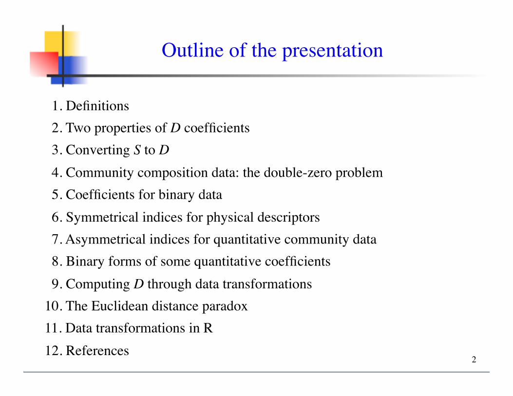
Outline of the presentation
1. Definitions 2. Two properties of D coefficients 3. Converting S to D 4. Community composition data: the double-zero problem 5. Coefficients for binary data 6. Symmetrical indices for physical descriptors 7. Asymmetrical indices for quantitative community data 8. Binary forms of some quantitative coefficients 9. Computing D through data transformations10. The Euclidean distance paradox11. Data transformations in R12. References
2
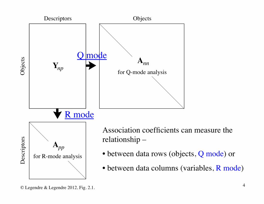
An association coefficient is a function of two data vectors that quantifies the strength of their relationship (or association).
Definitions
Dissimilarity 3
Ynp
DescriptorsD
escr
ipto
rsObjects
Obj
ects Ann
for Q-mode analysis
Appfor R-mode analysis
Association coefficients can measure the relationship –
• between data rows (objects, Q mode) or
• between data columns (variables, R mode)
Q mode
R mode
© Legendre & Legendre 2012, Fig. 2.1. 4
Q-mode coefficients (between objects, e.g. sites) are called similarities (S) and dissimilarities (D) 1.
R-mode coefficients (between descriptors or variables) are called dependence coefficients (correlation coefficients, contingency, ...)
In Q mode, one obtains a S or D matrix by computing similarities (S) or dissimilarities (D) between all pairs of sites.
In R mode, one obtains an R matrix by computing correlation coefficients between all pairs of columns.
1 Dissimilarities are often called distance coefficients. Technically, distances are metric dissimilarities (metric properties: described below).
Dissimilarity 5
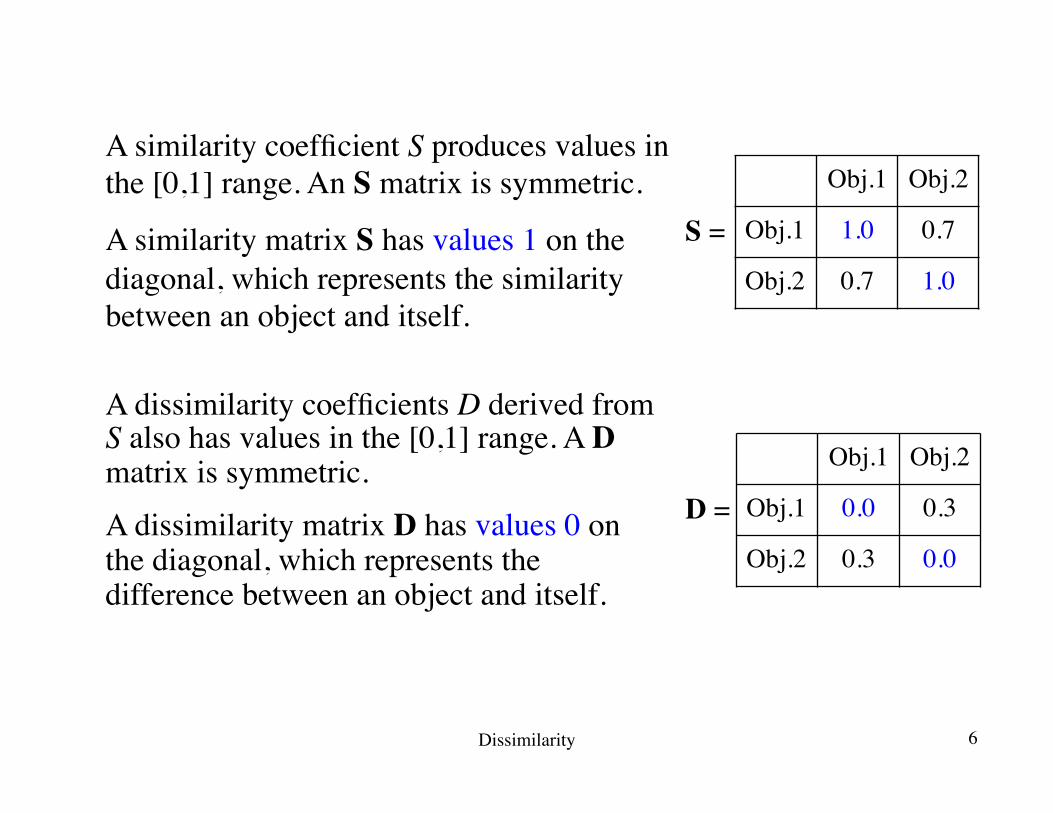
A similarity coefficient S produces values in the [0,1] range. An S matrix is symmetric.
A similarity matrix S has values 1 on the diagonal, which represents the similarity between an object and itself.
Obj.1 Obj.2
Obj.1 1.0 0.7
Obj.2 0.7 1.0
A dissimilarity coefficients D derived from S also has values in the [0,1] range. A D matrix is symmetric.
A dissimilarity matrix D has values 0 on the diagonal, which represents the difference between an object and itself.
S =
Obj.1 Obj.2
Obj.1 0.0 0.3
Obj.2 0.3 0.0
D =
Dissimilarity 6
In this presentation, we will focus on Q-mode coefficients –
In the R language, all association matrices computed with Q-mode coefficients are presented as D matrices. They contain either dissimilarity indices, or similarity indices transformed into dissimilarities (more details below).
A D function imposes a model onto the data. It filters the information of the data matrix Y, emphasizing a portion of the information and discarding other portions.
The (dis)similarity indices are not interchangeable. Users must know what information is emphasized (i.e. retained) and discarded (i.e. filtered out) by each type of S or D function.
Dissimilarity 7
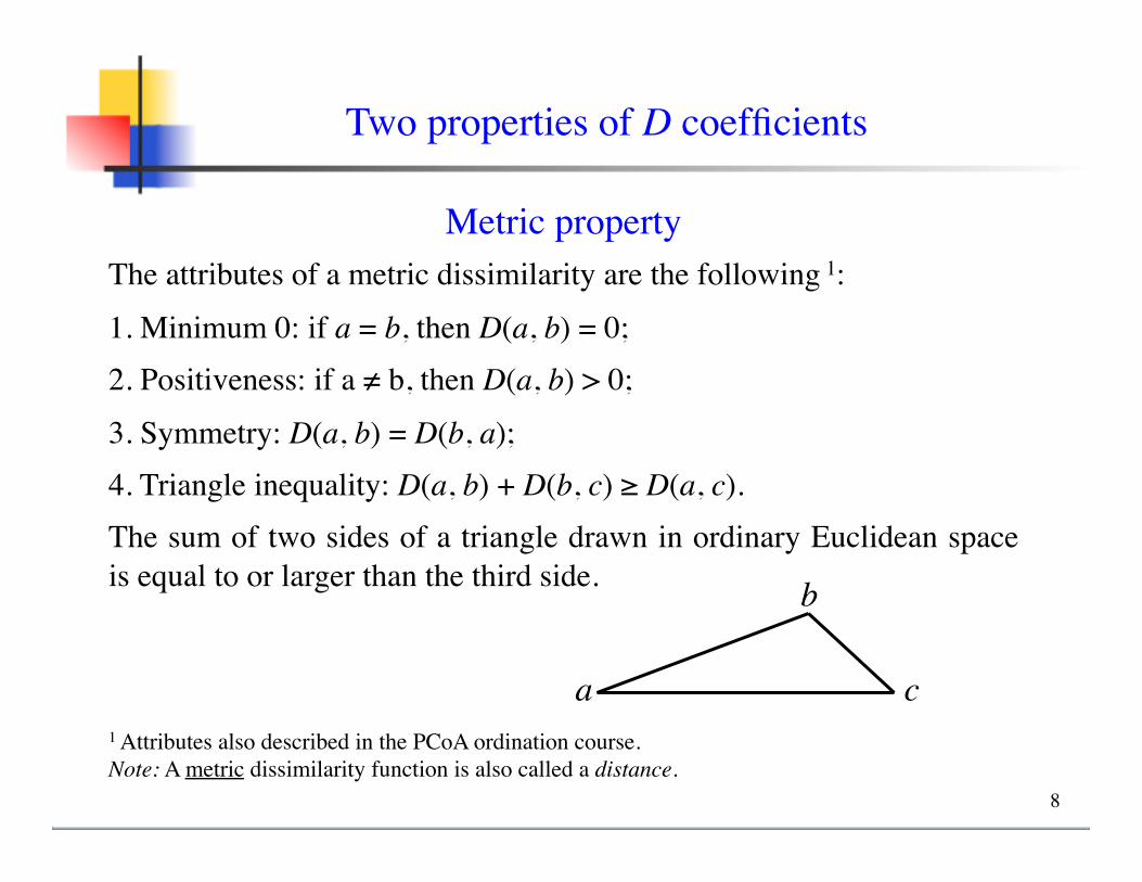
Metric propertyThe attributes of a metric dissimilarity are the following 1:
1. Minimum 0: if a = b, then D(a, b) = 0;2. Positiveness: if a ≠ b, then D(a, b) > 0;
3. Symmetry: D(a, b) = D(b, a);4. Triangle inequality: D(a, b) + D(b, c) ≥ D(a, c). The sum of two sides of a triangle drawn in ordinary Euclidean space is equal to or larger than the third side.
1 Attributes also described in the PCoA ordination course.Note: A metric dissimilarity function is also called a distance.
Two properties of D coefficients
a c
b
8
By reference to the attributes of a metric,
3 types of coefficients can be defined:
• metric: have all 4 attributes
• semimetric: can violate the triangle inequality
• nonmetric: can violate attributes 1–3. An example of a nonmetric coefficient will be presented later. These coefficients are not used in ecology.
Dissimilarity 9
Euclidean property 1
A dissimilarity coefficient is Euclidean if any resulting D matrix can be fully represented in a Euclidean space without distortion.
A non-Euclidean dissimilarity matrix is identified by the criterion that PCoA of that matrix produces some negative eigenvalues.
Taking the square root of most non-Euclidean D matrices makes them metric and Euclidean.
1 Property described in more detail in the principal coordinate analysis (PCoA) course. 10
Coefficients were originally described as either S or D.
Among the possible transformations from S to D, two are used in ecological analysis:
• D = 1 – S
• D = sqrt(1 – S)
In PCoA and in the distance-based approach to RDA (dbRDA), it is useful to make sure that the D matrix is Euclidean;
• use D = (1 – S) when (1 – S) is Euclidean;
• use D = sqrt(1 – S) when (1 – S) is not Euclidean but sqrt(1 – S) is Euclidean.
Converting S to D
Dissimilarity 11
=> Examine the metric and Euclidean properties of similarity and dissimilarity coefficients in Tables 9.2 and 9.3 of the Numerical ecology book. See complementary material, file “Legendre_&_Legendre_2012_Tables_7.2+7.3.pdf”.
In most cases, sqrt(D) or sqrt(1 – S) turns a non-Euclidean matrix into Euclidean.
More about this in the course on principal coordinate analysis (PCoA).
Dissimilarity 12
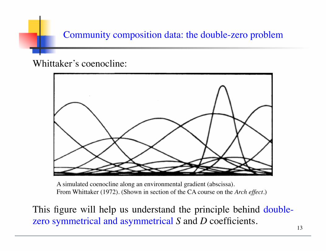
Whittaker’s coenocline:
Community composition data: the double-zero problem
A simulated coenocline along an environmental gradient (abscissa). From Whittaker (1972). (Shown in section of the CA course on the Arch effect.)
This figure will help us understand the principle behind double-zero symmetrical and asymmetrical S and D coefficients.
13
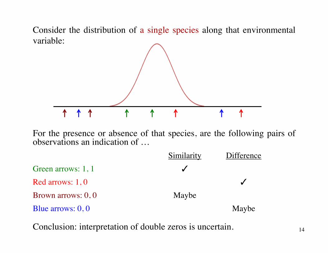
Consider the distribution of a single species along that environmental variable:
For the presence or absence of that species, are the following pairs of observations an indication of …
Similarity DifferenceGreen arrows: 1, 1 ✓
Red arrows: 1, 0 ✓
Brown arrows: 0, 0 MaybeBlue arrows: 0, 0 Maybe
Conclusion: interpretation of double zeros is uncertain. 14
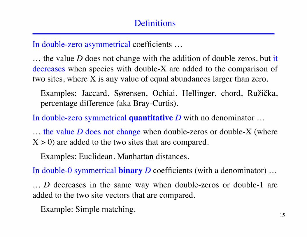
Definitions
In double-zero asymmetrical coefficients …… the value D does not change with the addition of double zeros, but it decreases when species with double-X are added to the comparison of two sites, where X is any value of equal abundances larger than zero.
Examples: Jaccard, Sørensen, Ochiai, Hellinger, chord, Ružička, percentage difference (aka Bray-Curtis).
In double-zero symmetrical quantitative D with no denominator …… the value D does not change when double-zeros or double-X (where X > 0) are added to the two sites that are compared.
Examples: Euclidean, Manhattan distances.In double-0 symmetrical binary D coefficients (with a denominator) …
… D decreases in the same way when double-zeros or double-1 are added to the two site vectors that are compared.
Example: Simple matching. 15
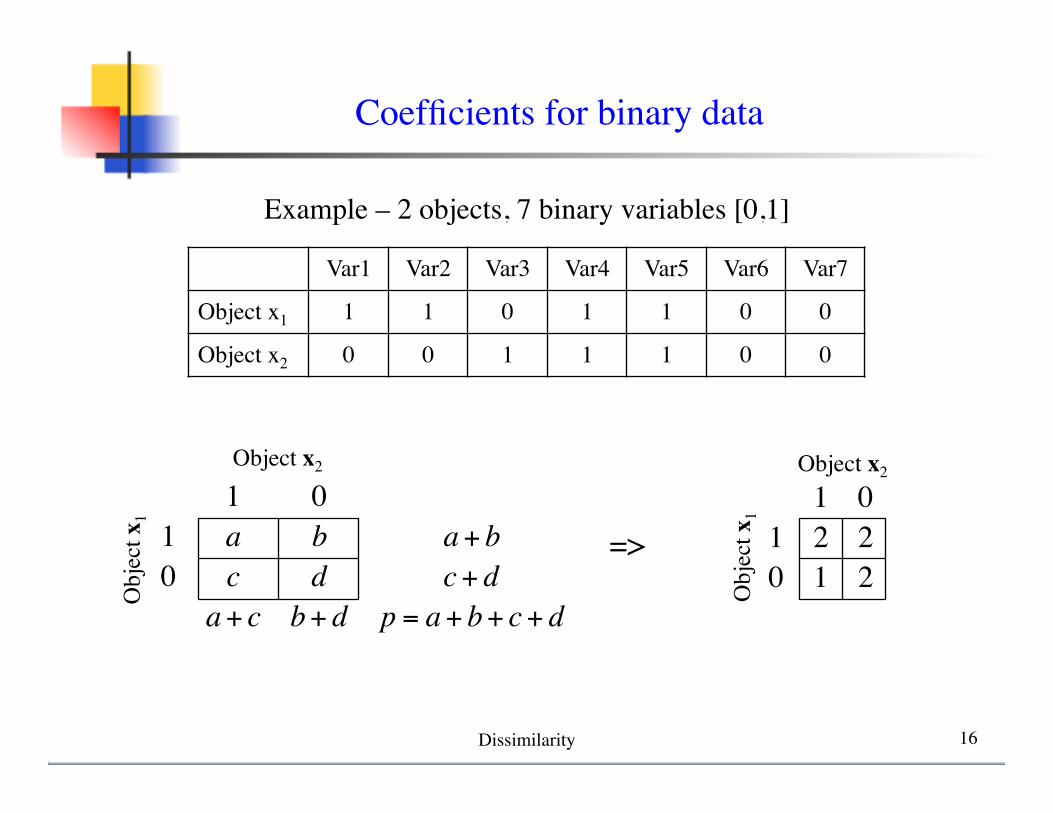
1 01 a b a+ b0 c d c+ d
a+ c b+ d p = a+ b+ c+ d
Object x2
Obj
ect x
1
Var1 Var2 Var3 Var4 Var5 Var6 Var7
Object x1 1 1 0 1 1 0 0
Object x2 0 0 1 1 1 0 0
Example – 2 objects, 7 binary variables [0,1]
=>1 0
1 2 20 1 2
Object x2
Obj
ect x
1
Coefficients for binary data
Dissimilarity 16
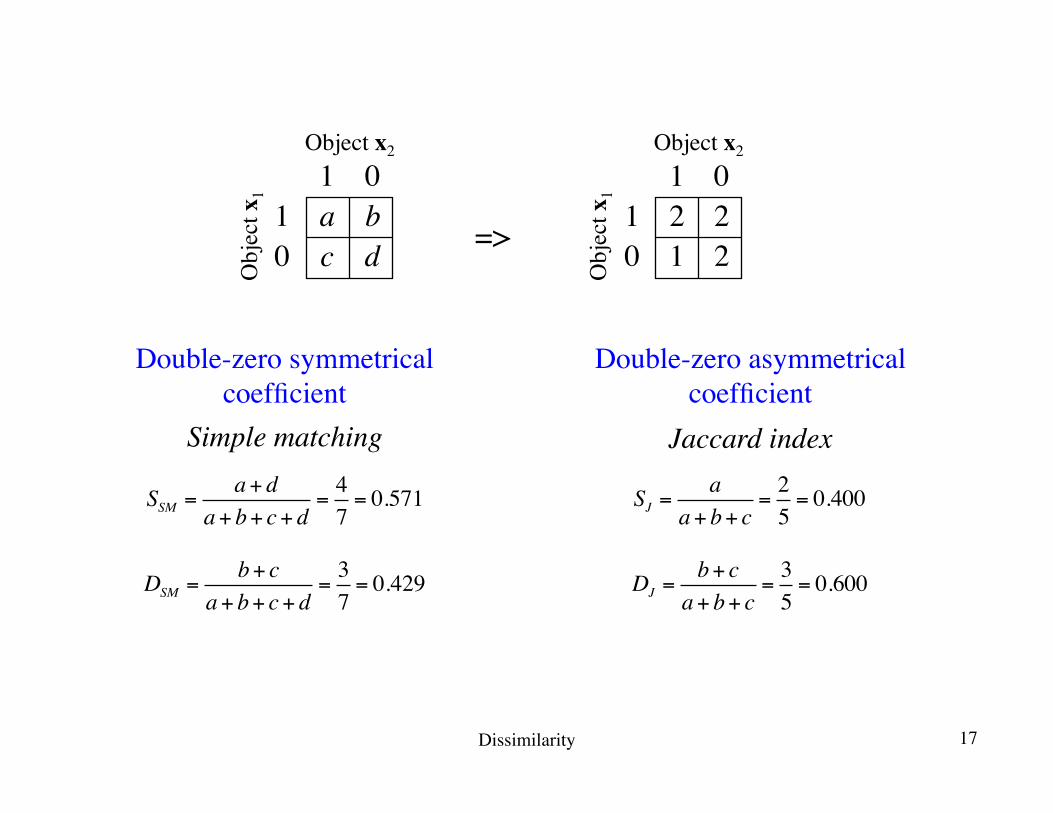
SJ =a
a+ b+ c=25= 0.400SSM =
a+ da+ b+ c+ d
=47= 0.571
=>
1 01 2 20 1 2
Object x2
Obj
ect x
1
1 01 a b0 c d
Object x2
Obj
ect x
1
Double-zero symmetricalcoefficient
Double-zero asymmetricalcoefficient
DSM =b+ c
a+ b+ c+ d=37= 0.429 DJ =
b+ ca+ b+ c
=35= 0.600
Simple matching Jaccard index
Dissimilarity 17
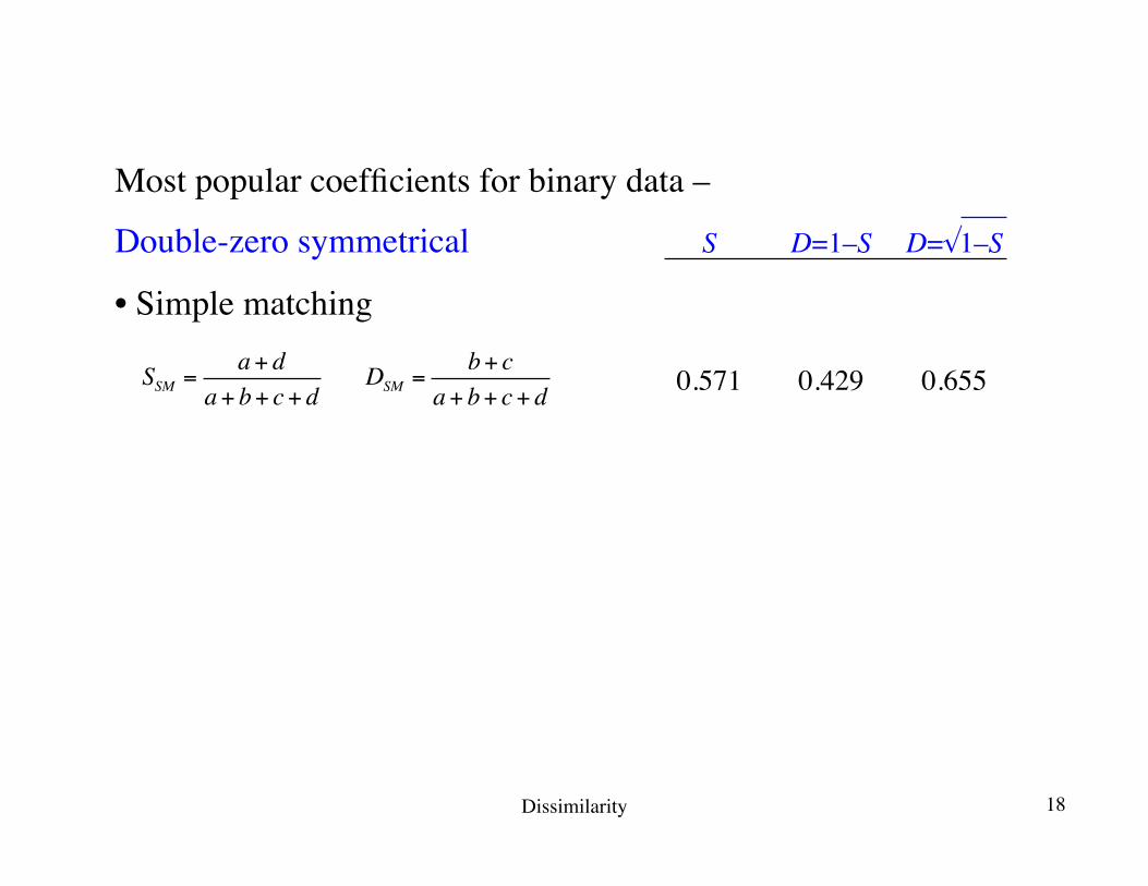
Most popular coefficients for binary data –
Double-zero symmetrical S D=1–S D=√1–S
• Simple matching
0.571 0.429 0.655SSM =a+ d
a+ b+ c+ dDSM =
b+ ca+ b+ c+ d
Dissimilarity 18
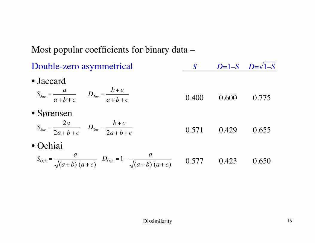
Most popular coefficients for binary data –
Double-zero asymmetrical S D=1–S D=√1–S
• Jaccard
0.400 0.600 0.775
• Sørensen
0.571 0.429 0.655
• Ochiai0.577 0.423 0.650
SJac =a
a+ b+ c
SSor =2a
2a+ b+ c
SOch =a
(a+ b) (a+ c)
DJac =b+ c
a+ b+ c
DSor =b+ c
2a+ b+ c
DOch =1−a
(a+ b) (a+ c)
Dissimilarity 19
SJ =a
a+ b+ c=25= 0.400SSM =
a+ da+ b+ c+ d
=710
= 0.700
=>
1 01 2 20 1 5
Object x2
Obj
ect x
1
1 01 a b0 c d
Object x2
Obj
ect x
1
DSM =b+ c
a+ b+ c+ d=310
= 0.300 DJ =b+ c
a+ b+ c=35= 0.600
Simple matching Jaccard index
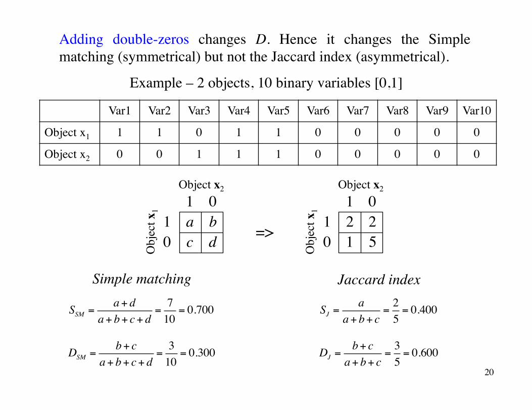
Adding double-zeros changes D. Hence it changes the Simple matching (symmetrical) but not the Jaccard index (asymmetrical).
Var1 Var2 Var3 Var4 Var5 Var6 Var7 Var8 Var9 Var10
Object x1 1 1 0 1 1 0 0 0 0 0
Object x2 0 0 1 1 1 0 0 0 0 0
Example – 2 objects, 10 binary variables [0,1]
20
This example shows that double-zero asymmetrical indices are insensitive to double-zeros, i.e. the absence of species at two sites, …
… because the value d is not included in their formula.
However, double-presences (a) do change the denominator, hence they change the index value.
These indices are well suited to the analysis of community composition or other types of frequency data, e.g. gene frequencies.
Double-zero symmetrical indices are not adapted to the analysis of these types of data.
Dissimilarity 21
10 different forms of binary indices (for presence-absence data) are available in dist.binary of {ade4} in R.
The three most widely used binary indices, i.e. Jaccard, Sørensen and Ochiai, are also available in dist.ldc of {adespatial}.
Note: When computing binary indices in these two packages, these similarities (S) are converted to distances through the transformation .
The transformation is automatically applied because it makes the D matrices Euclidean.
Euclidean matrices will not produce negative eigenvalues in PCoA. Refer to the PCoA course.
D = 1− S
Dissimilarity 22
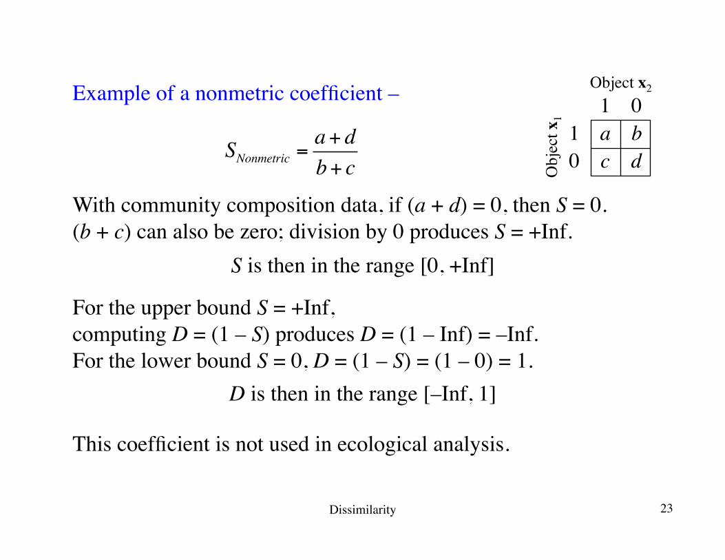
Example of a nonmetric coefficient –
With community composition data, if (a + d) = 0, then S = 0. (b + c) can also be zero; division by 0 produces S = +Inf.
S is then in the range [0, +Inf]
For the upper bound S = +Inf, computing D = (1 – S) produces D = (1 – Inf) = –Inf.For the lower bound S = 0, D = (1 – S) = (1 – 0) = 1.
D is then in the range [–Inf, 1]
This coefficient is not used in ecological analysis.
SNonmetric =a+ db+ c
1 01 a b0 c d
Object x2
Obj
ect x
1
Dissimilarity 23
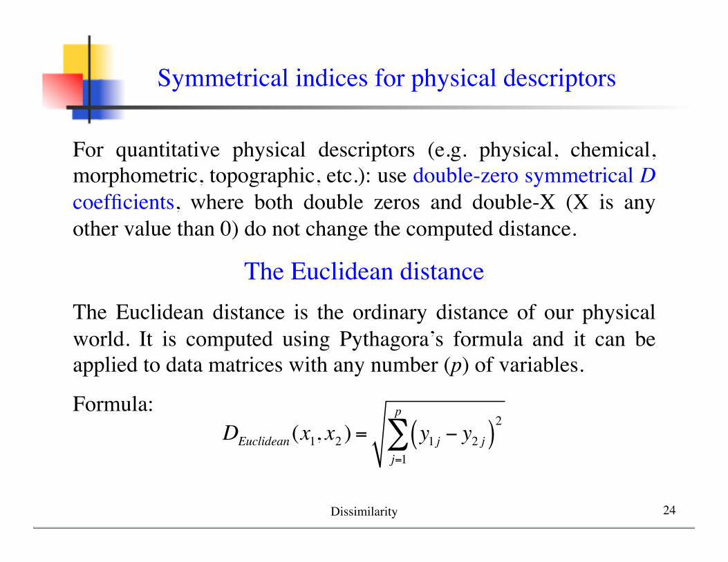
For quantitative physical descriptors (e.g. physical, chemical, morphometric, topographic, etc.): use double-zero symmetrical D coefficients, where both double zeros and double-X (X is any other value than 0) do not change the computed distance.
The Euclidean distanceThe Euclidean distance is the ordinary distance of our physical world. It is computed using Pythagora’s formula and it can be applied to data matrices with any number (p) of variables.
Formula:
Symmetrical indices for physical descriptors
DEuclidean (x1, x2 ) = y1 j − y2 j( )2
j=1
p
∑
Dissimilarity 24
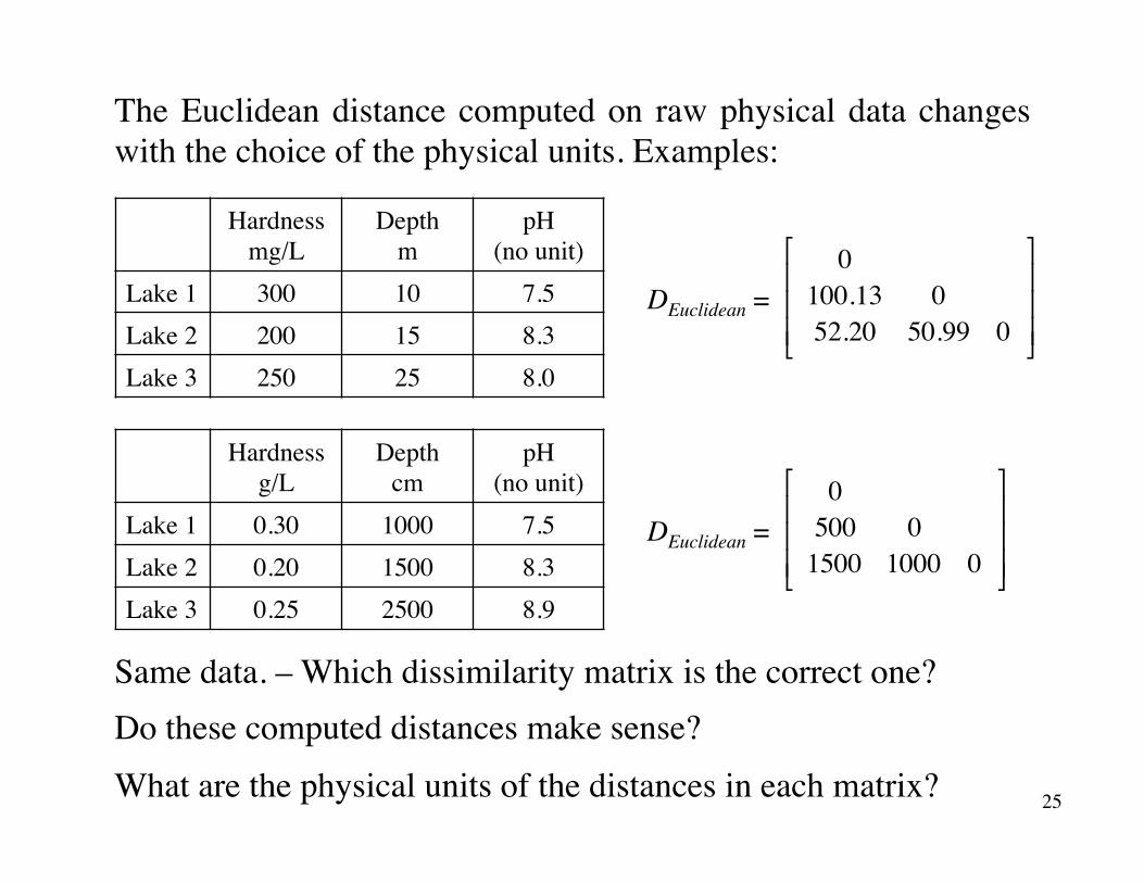
The Euclidean distance computed on raw physical data changes with the choice of the physical units. Examples:
Hardnessg/L
Depthcm
pH(no unit)
Lake 1 0.30 1000 7.5Lake 2 0.20 1500 8.3Lake 3 0.25 2500 8.9
Same data. – Which dissimilarity matrix is the correct one?Do these computed distances make sense?
What are the physical units of the distances in each matrix?
DEuclidean =
Hardnessmg/L
Depthm
pH(no unit)
Lake 1 300 10 7.5Lake 2 200 15 8.3Lake 3 250 25 8.0
0100.13 052.20 50.99 0
⎡
⎣
⎢⎢⎢
⎤
⎦
⎥⎥⎥
DEuclidean =0500 01500 1000 0
⎡
⎣
⎢⎢⎢
⎤
⎦
⎥⎥⎥
25
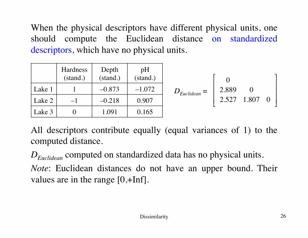
When the physical descriptors have different physical units, one should compute the Euclidean distance on standardized descriptors, which have no physical units.
DEuclidean =
Hardness(stand.)
Depth(stand.)
pH(stand.)
Lake 1 1 –0.873 –1.072Lake 2 –1 –0.218 0.907Lake 3 0 1.091 0.165
02.889 02.527 1.807 0
⎡
⎣
⎢⎢⎢
⎤
⎦
⎥⎥⎥
All descriptors contribute equally (equal variances of 1) to the computed distance.DEuclidean computed on standardized data has no physical units.Note: Euclidean distances do not have an upper bound. Their values are in the range [0,+Inf].
Dissimilarity 26
Do not compute DEuclidean on raw (untransformed) community composition data, standardized or not.There are, however, transformations that are appropriate for community data before computing the Euclidean distance. They are described later in this presentation.
Dissimilarity 27
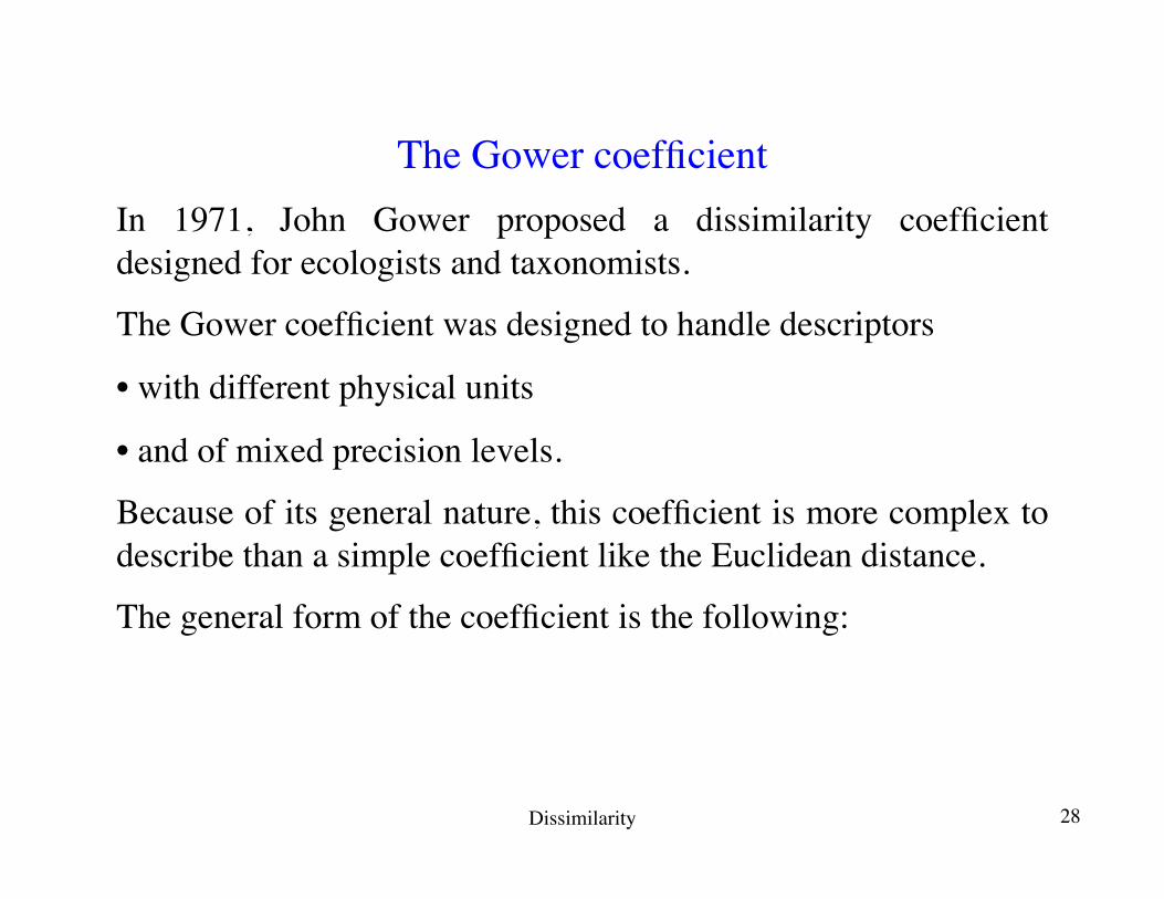
The Gower coefficientIn 1971, John Gower proposed a dissimilarity coefficient designed for ecologists and taxonomists.
The Gower coefficient was designed to handle descriptors
• with different physical units
• and of mixed precision levels.
Because of its general nature, this coefficient is more complex to describe than a simple coefficient like the Euclidean distance.
The general form of the coefficient is the following:
Dissimilarity 28
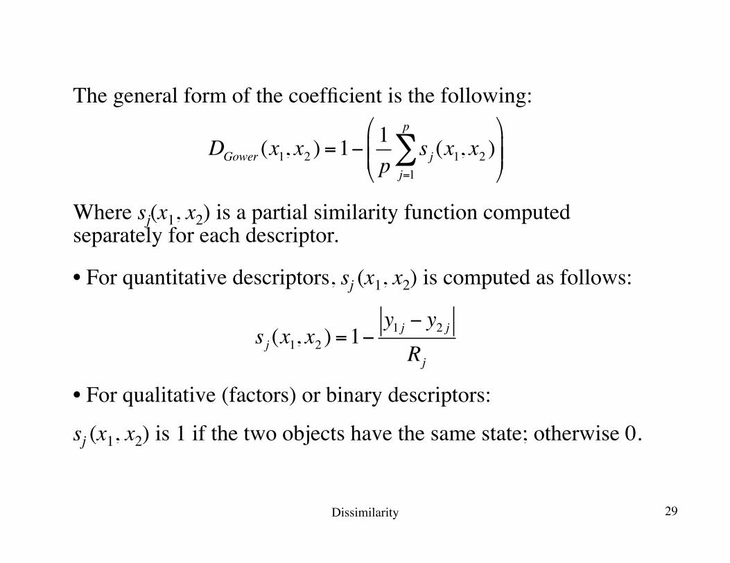
The general form of the coefficient is the following:
DGower (x1, x2 ) =1−1p
sj (x1, x2 )j=1
p
∑⎛
⎝⎜⎜
⎞
⎠⎟⎟
Where sj(x1, x2) is a partial similarity function computed separately for each descriptor.
• For quantitative descriptors, sj (x1, x2) is computed as follows:
sj (x1, x2 ) =1−y1 j − y2 jRj
• For qualitative (factors) or binary descriptors:
sj (x1, x2) is 1 if the two objects have the same state; otherwise 0.
Dissimilarity 29
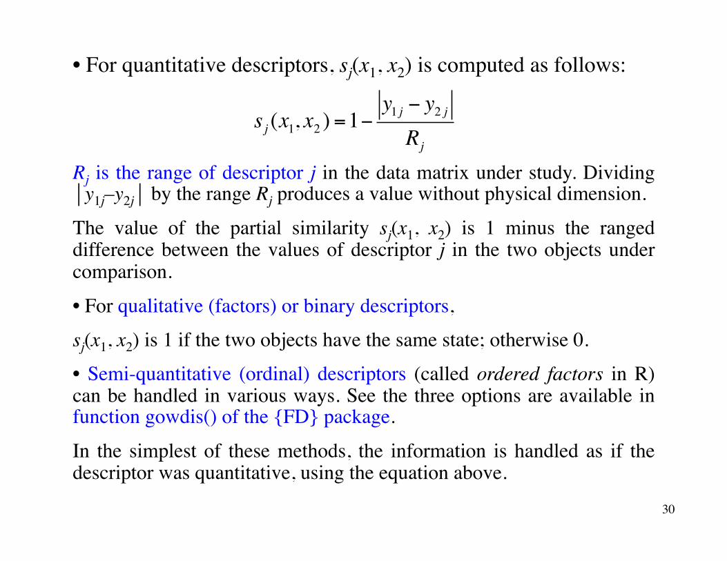
• For quantitative descriptors, sj(x1, x2) is computed as follows:
sj (x1, x2 ) =1−y1 j − y2 jRj
Rj is the range of descriptor j in the data matrix under study. Dividing ⏐y1j–y2j⏐ by the range Rj produces a value without physical dimension.
The value of the partial similarity sj(x1, x2) is 1 minus the ranged difference between the values of descriptor j in the two objects under comparison.
• For qualitative (factors) or binary descriptors,
sj(x1, x2) is 1 if the two objects have the same state; otherwise 0.
• Semi-quantitative (ordinal) descriptors (called ordered factors in R) can be handled in various ways. See the three options are available in function gowdis() of the {FD} package.
In the simplest of these methods, the information is handled as if the descriptor was quantitative, using the equation above.
30
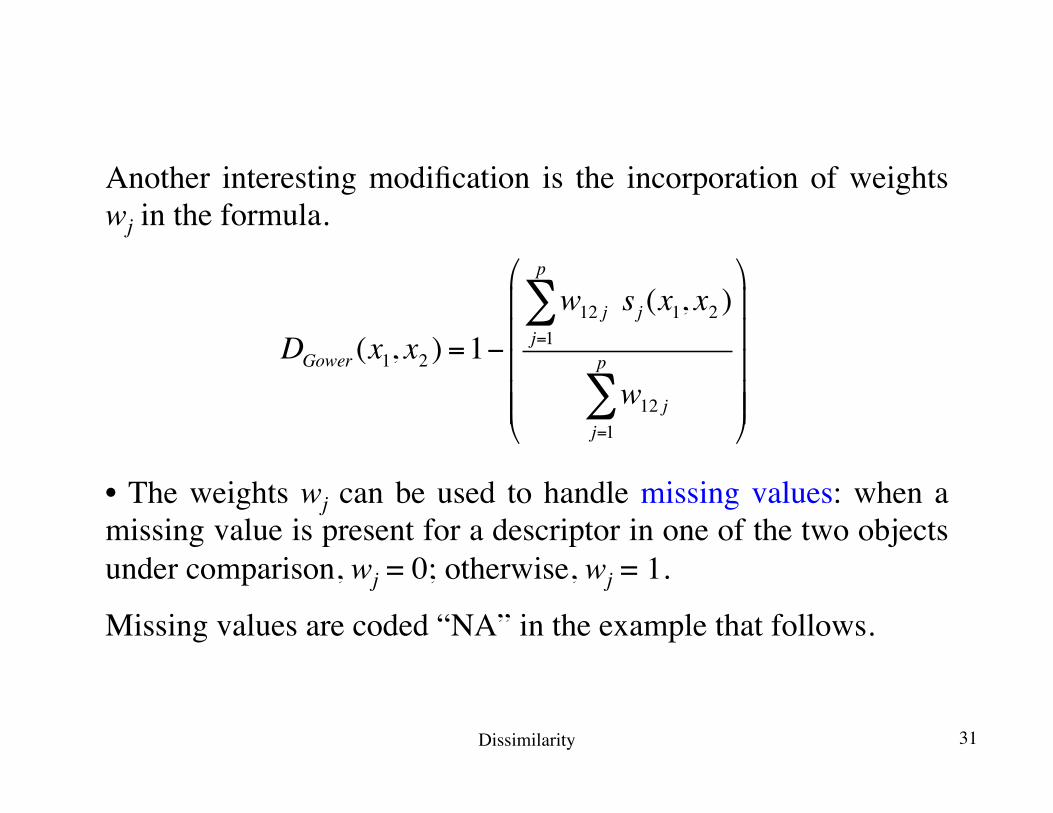
Another interesting modification is the incorporation of weights wj in the formula.
• The weights wj can be used to handle missing values: when a missing value is present for a descriptor in one of the two objects under comparison, wj = 0; otherwise, wj = 1.
Missing values are coded “NA” in the example that follows.
DGower (x1, x2 ) =1−w12 j sj (x1, x2 )
j=1
p
∑
w12 jj=1
p
∑
⎛
⎝
⎜⎜⎜⎜⎜
⎞
⎠
⎟⎟⎟⎟⎟
Dissimilarity 31
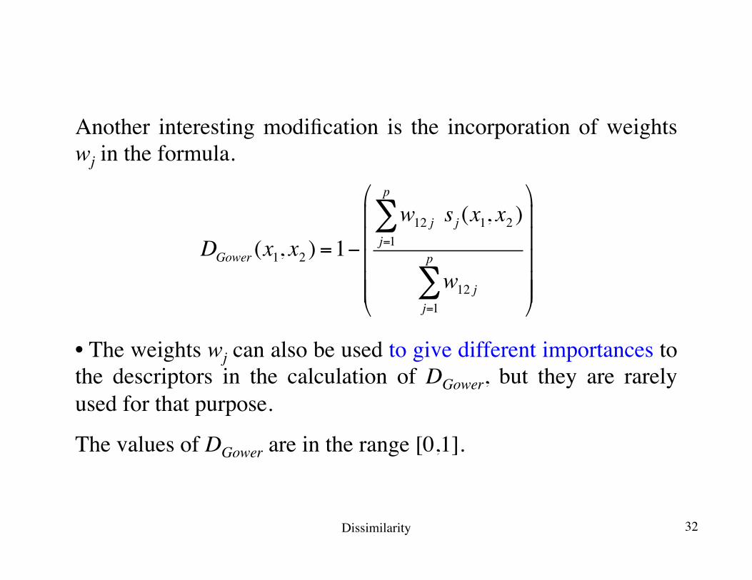
Another interesting modification is the incorporation of weights wj in the formula.
• The weights wj can also be used to give different importances to the descriptors in the calculation of DGower, but they are rarely used for that purpose.
The values of DGower are in the range [0,1].
DGower (x1, x2 ) =1−w12 j sj (x1, x2 )
j=1
p
∑
w12 jj=1
p
∑
⎛
⎝
⎜⎜⎜⎜⎜
⎞
⎠
⎟⎟⎟⎟⎟
Dissimilarity 32
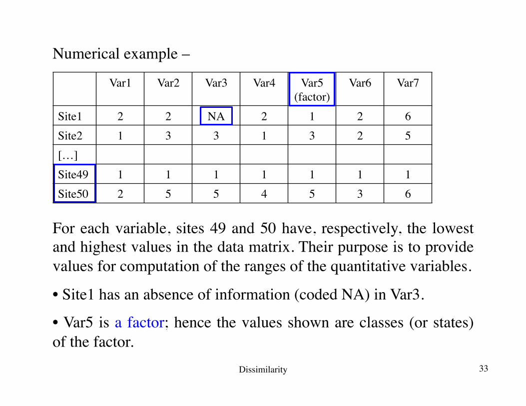
Numerical example –
For each variable, sites 49 and 50 have, respectively, the lowest and highest values in the data matrix. Their purpose is to provide values for computation of the ranges of the quantitative variables.
• Site1 has an absence of information (coded NA) in Var3.
• Var5 is a factor; hence the values shown are classes (or states) of the factor.
Var1 Var2 Var3 Var4 Var5(factor)
Var6 Var7
Site1 2 2 NA 2 1 2 6Site2 1 3 3 1 3 2 5[…]Site49 1 1 1 1 1 1 1Site50 2 5 5 4 5 3 6
Dissimilarity 33
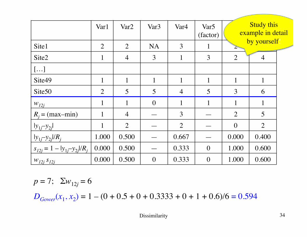
p = 7; Σw12j = 6
DGower(x1, x2) = 1 – (0 + 0.5 + 0 + 0.3333 + 0 + 1 + 0.6)/6 = 0.594
Var1 Var2 Var3 Var4 Var5(factor)
Var6 Var7
Site1 2 2 NA 3 1 2 6Site2 1 4 3 1 3 2 4[…]Site49 1 1 1 1 1 1 1Site50 2 5 5 4 5 3 6w12j 1 1 0 1 1 1 1Rj = (max–min) 1 4 — 3 — 2 5|y1j–y2j| 1 2 — 2 — 0 2|y1j–y2j|/Rj 1.000 0.500 — 0.667 — 0.000 0.400s12j = 1 – |y1j–y2j|/Rj 0.000 0.500 — 0.333 0 1.000 0.600w12j s12j 0.000 0.500 0 0.333 0 1.000 0.600
Study this example in detail
by yourself!
Dissimilarity 34
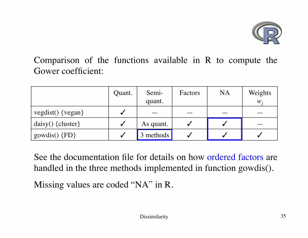
Comparison of the functions available in R to compute the Gower coefficient:
Quant. Semi-quant.
Factors NA Weightswj
vegdist() {vegan} ✓ — — — —daisy() {cluster} ✓ As quant. ✓ ✓ —gowdis() {FD} ✓ 3 methods ✓ ✓ ✓
See the documentation file for details on how ordered factors are handled in the three methods implemented in function gowdis().
Missing values are coded “NA” in R.
Dissimilarity 35
I will now focus on seven double-zero asymmetrical dissimilarity coefficients for quantitative community composition data, and mention some others.
Quantitative community data: asymmetrical indices
Dissimilarity 36
The first two indices for quantitative community data are the quantitative forms of the Jaccard and Sørensen indices for binary data, described above.
These two indices are based on the same decomposition of the species abundance data.
The calculation of dissimilarity incorporates the differences in total abundance of the sites.
The data are not scaled by rows, as will be the case in the next series of indices. The differences in productivity of the sites are taken into account in the calculation of the dissimilarities.
Asymmetrical non-Euclidean indices
Dissimilarity 37
Spec.1 Spec.4Spec.3Spec.2
Site1 Site2 Site1 Site2 Site1 Site2 Site1 Site2
A = abun. common to sites 1 and 2 = A1+A2+0+A4B = abundances unique to site 1 = 0+B2+B3+0C = abundances unique to site 2 = C1+0+0+0
A1 A1 A2 A2
A4 A4B2
B3
C1
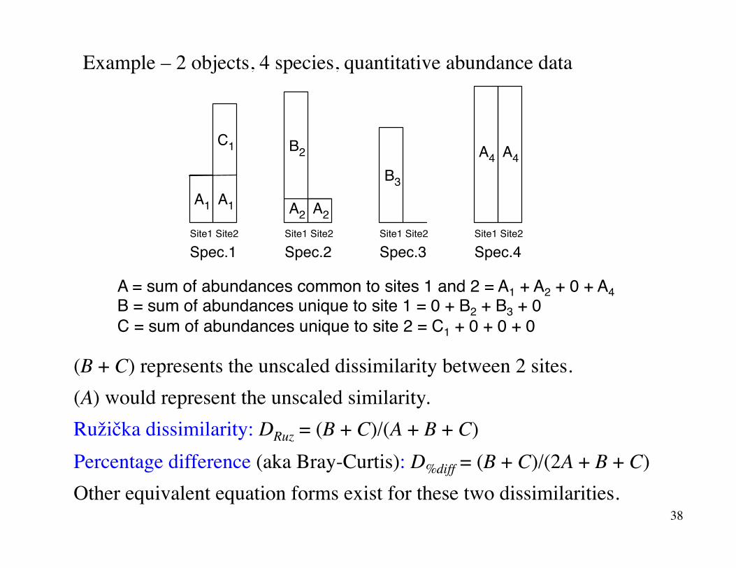
Example – 2 objects, 4 species, quantitative abundance data
(B + C) represents the unscaled dissimilarity between 2 sites.(A) would represent the unscaled similarity.Ružička dissimilarity: DRuz = (B + C)/(A + B + C)Percentage difference (aka Bray-Curtis): D%diff = (B + C)/(2A + B + C)Other equivalent equation forms exist for these two dissimilarities.
A = sum of abundances common to sites 1 and 2 = A1 + A2 + 0 + A4B = sum of abundances unique to site 1 = 0 + B2 + B3 + 0C = sum of abundances unique to site 2 = C1 + 0 + 0 + 0
38
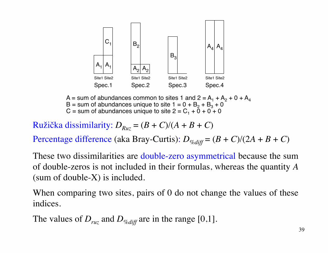
Ružička dissimilarity: DRuz = (B + C)/(A + B + C)Percentage difference (aka Bray-Curtis): D%diff = (B + C)/(2A + B + C)
Spec.1 Spec.4Spec.3Spec.2
Site1 Site2 Site1 Site2 Site1 Site2 Site1 Site2
A = abun. common to sites 1 and 2 = A1+A2+0+A4B = abundances unique to site 1 = 0+B2+B3+0C = abundances unique to site 2 = C1+0+0+0
A1 A1 A2 A2
A4 A4B2
B3
C1
A = sum of abundances common to sites 1 and 2 = A1 + A2 + 0 + A4B = sum of abundances unique to site 1 = 0 + B2 + B3 + 0C = sum of abundances unique to site 2 = C1 + 0 + 0 + 0
These two dissimilarities are double-zero asymmetrical because the sum of double-zeros is not included in their formulas, whereas the quantity A (sum of double-X) is included.
When comparing two sites, pairs of 0 do not change the values of these indices.
The values of Druz and D%diff are in the range [0,1].39
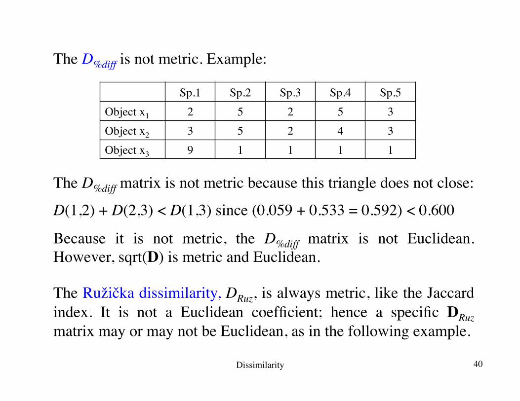
The D%diff is not metric. Example:
Sp.1 Sp.2 Sp.3 Sp.4 Sp.5Object x1 2 5 2 5 3Object x2 3 5 2 4 3Object x3 9 1 1 1 1
The D%diff matrix is not metric because this triangle does not close:
D(1,2) + D(2,3) < D(1,3) since (0.059 + 0.533 = 0.592) < 0.600
Because it is not metric, the D%diff matrix is not Euclidean. However, sqrt(D) is metric and Euclidean. The Ružička dissimilarity, DRuz, is always metric, like the Jaccard index. It is not a Euclidean coefficient; hence a specific DRuz matrix may or may not be Euclidean, as in the following example.
Dissimilarity 40
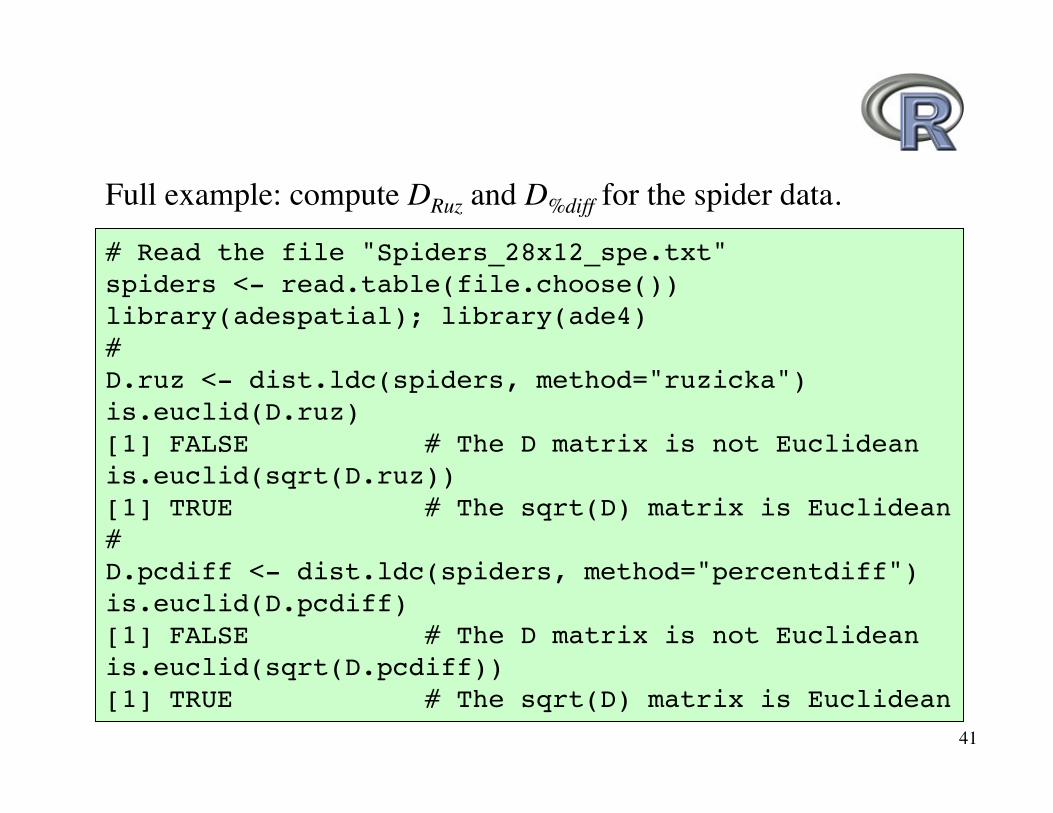
Full example: compute DRuz and D%diff for the spider data.
# Read the file "Spiders_28x12_spe.txt" spiders <- read.table(file.choose())library(adespatial); library(ade4)#D.ruz <- dist.ldc(spiders, method="ruzicka")is.euclid(D.ruz)[1] FALSE # The D matrix is not Euclideanis.euclid(sqrt(D.ruz))[1] TRUE # The sqrt(D) matrix is Euclidean#D.pcdiff <- dist.ldc(spiders, method="percentdiff")is.euclid(D.pcdiff)[1] FALSE # The D matrix is not Euclideanis.euclid(sqrt(D.pcdiff))[1] TRUE # The sqrt(D) matrix is Euclidean
41
Historical noteThe percentage difference
D%diff = (B + C)/(2A + B + C)was described by Odum in 1950.This D index is often called the Bray-Curtis index in computer software. This is a misnomer, repeating a mistake in a paper published around 1970.The 1957 paper by Bray & Curtis aimed at describing a new ordination method, known as the Bray-Curtis ordination, not a new D index.Actually, the index used by Bray and Curtis in their 1957 paper, and clearly described on p. 329, is Whittaker’s (1952) index of association.
Dissimilarity 42
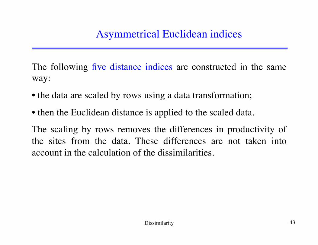
The following five distance indices are constructed in the same way:
• the data are scaled by rows using a data transformation;
• then the Euclidean distance is applied to the scaled data.
The scaling by rows removes the differences in productivity of the sites from the data. These differences are not taken into account in the calculation of the dissimilarities.
Asymmetrical Euclidean indices
Dissimilarity 43
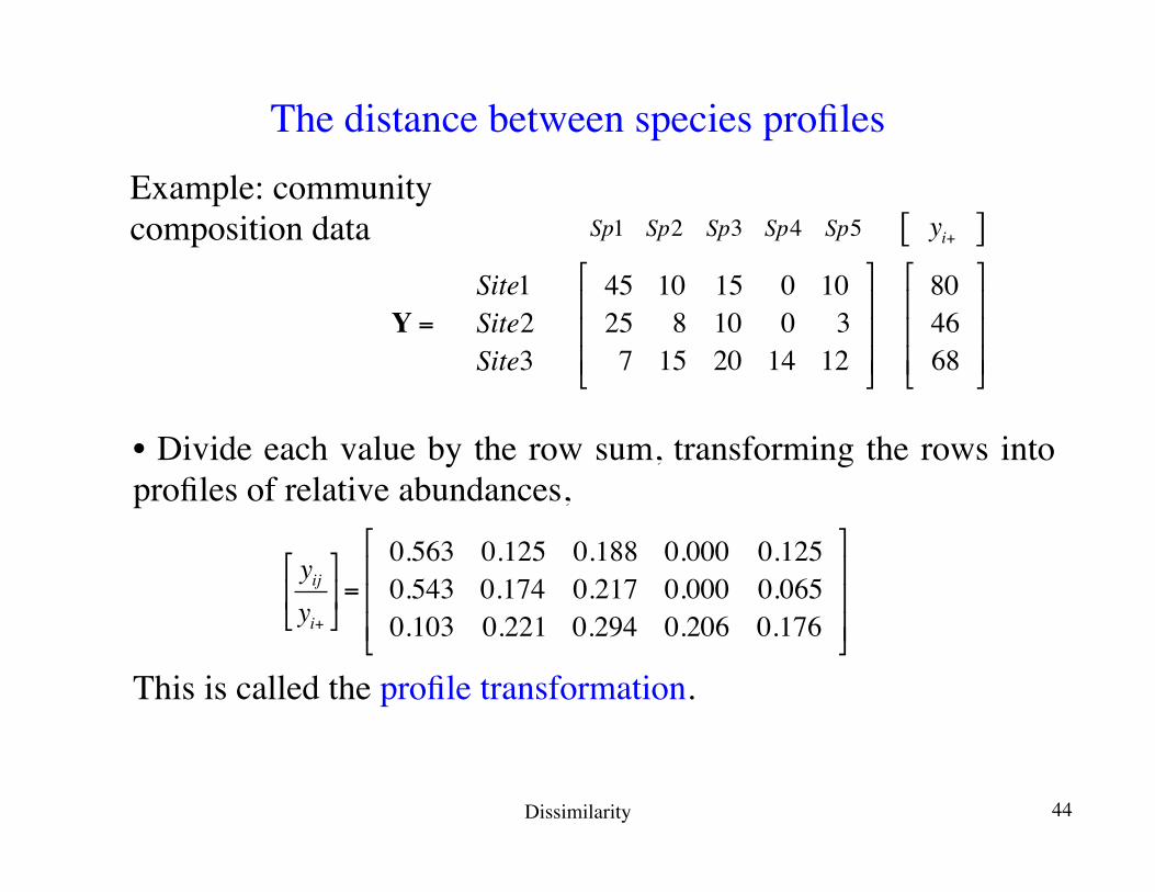
The distance between species profiles Example: community composition data Sp1 Sp2 Sp3 Sp4 Sp5 yi+ [ ]
Y =Site1Site2Site3
45 10 15 0 1025 8 10 0 37 15 20 14 12
⎡
⎣
⎢⎢⎢
⎤
⎦
⎥⎥⎥
804668
⎡
⎣
⎢⎢⎢
⎤
⎦
⎥⎥⎥
• Divide each value by the row sum, transforming the rows into profiles of relative abundances,
This is called the profile transformation.
yijyi+
⎡
⎣⎢
⎤
⎦⎥=
0.563 0.125 0.188 0.000 0.1250.543 0.174 0.217 0.000 0.0650.103 0.221 0.294 0.206 0.176
⎡
⎣
⎢⎢⎢
⎤
⎦
⎥⎥⎥
Dissimilarity 44
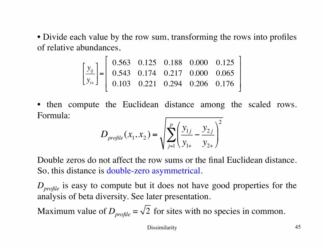
• Divide each value by the row sum, transforming the rows into profiles of relative abundances,
• then compute the Euclidean distance among the scaled rows. Formula:
Double zeros do not affect the row sums or the final Euclidean distance. So, this distance is double-zero asymmetrical.Dprofile is easy to compute but it does not have good properties for the analysis of beta diversity. See later presentation.Maximum value of Dprofile = for sites with no species in common.
Dprofile(x1, x2 ) =y1 jy1+
−y2 jy2+
⎛
⎝⎜
⎞
⎠⎟
2
j=1
p
∑
yijyi+
⎡
⎣⎢
⎤
⎦⎥=
0.563 0.125 0.188 0.000 0.1250.543 0.174 0.217 0.000 0.0650.103 0.221 0.294 0.206 0.176
⎡
⎣
⎢⎢⎢
⎤
⎦
⎥⎥⎥
2
Dissimilarity 45
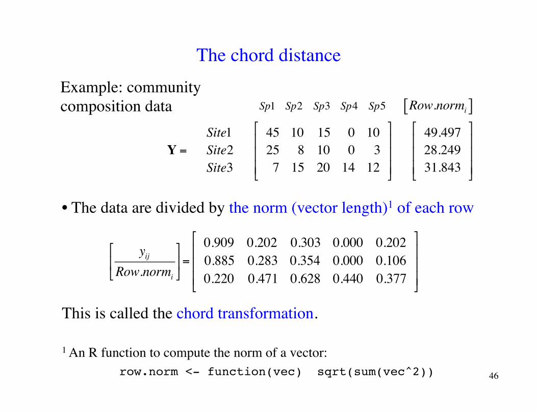
The chord distanceExample: community composition data Sp1 Sp2 Sp3 Sp4 Sp5 Row.normi[ ]
Y =Site1Site2Site3
45 10 15 0 1025 8 10 0 37 15 20 14 12
⎡
⎣
⎢⎢⎢
⎤
⎦
⎥⎥⎥
49.49728.24931.843
⎡
⎣
⎢⎢⎢
⎤
⎦
⎥⎥⎥
• The data are divided by the norm (vector length)1 of each row
yijRow.normi
⎡
⎣⎢
⎤
⎦⎥=
0.909 0.202 0.303 0.000 0.2020.885 0.283 0.354 0.000 0.1060.220 0.471 0.628 0.440 0.377
⎡
⎣
⎢⎢⎢
⎤
⎦
⎥⎥⎥
This is called the chord transformation.
1 An R function to compute the norm of a vector: row.norm <- function(vec) sqrt(sum(vec^2)) 46
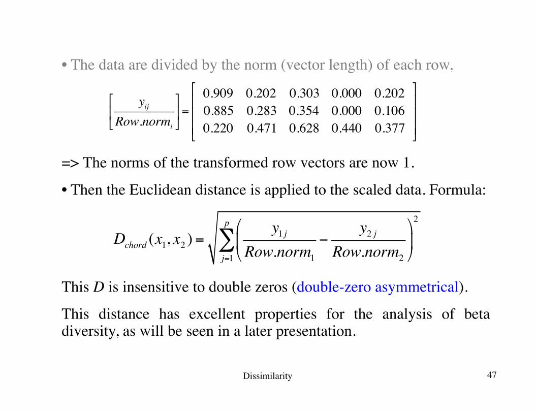
• The data are divided by the norm (vector length) of each row,
=> The norms of the transformed row vectors are now 1.
• Then the Euclidean distance is applied to the scaled data. Formula:
This D is insensitive to double zeros (double-zero asymmetrical).
This distance has excellent properties for the analysis of beta diversity, as will be seen in a later presentation.
Dchord (x1, x2 ) =y1 j
Row.norm1−
y2 jRow.norm2
⎛
⎝⎜
⎞
⎠⎟
2
j=1
p
∑
yijRow.normi
⎡
⎣⎢
⎤
⎦⎥=
0.909 0.202 0.303 0.000 0.2020.885 0.283 0.354 0.000 0.1060.220 0.471 0.628 0.440 0.377
⎡
⎣
⎢⎢⎢
⎤
⎦
⎥⎥⎥
Dissimilarity 47
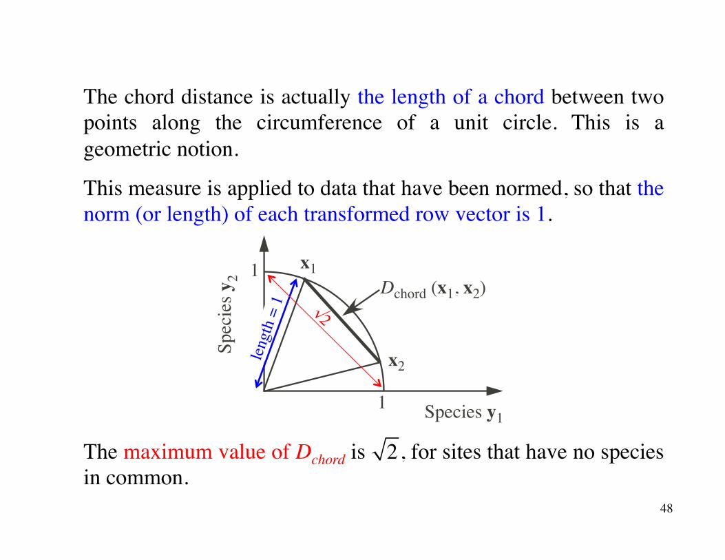
The chord distance is actually the length of a chord between two points along the circumference of a unit circle. This is a geometric notion.
This measure is applied to data that have been normed, so that the norm (or length) of each transformed row vector is 1.
Species y1
Spec
ies y
2
x1
x2
Dchord (x1, x2)1
1
The maximum value of Dchord is , for sites that have no species in common.
2
48
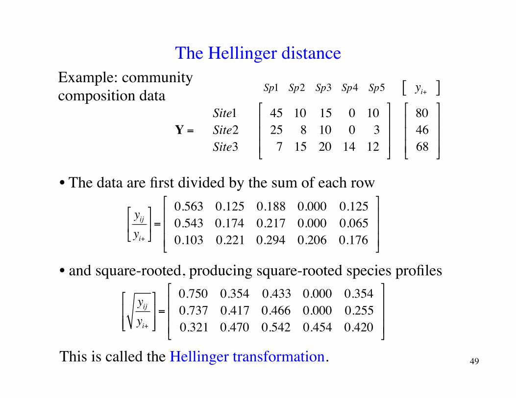
The Hellinger distanceExample: community composition data Sp1 Sp2 Sp3 Sp4 Sp5 yi+ [ ]
Y =Site1Site2Site3
45 10 15 0 1025 8 10 0 37 15 20 14 12
⎡
⎣
⎢⎢⎢
⎤
⎦
⎥⎥⎥
804668
⎡
⎣
⎢⎢⎢
⎤
⎦
⎥⎥⎥
• The data are first divided by the sum of each row
• and square-rooted, producing square-rooted species profiles
yijyi+
⎡
⎣⎢
⎤
⎦⎥=
0.563 0.125 0.188 0.000 0.1250.543 0.174 0.217 0.000 0.0650.103 0.221 0.294 0.206 0.176
⎡
⎣
⎢⎢⎢
⎤
⎦
⎥⎥⎥
yijyi+
⎡
⎣⎢⎢
⎤
⎦⎥⎥=
0.750 0.354 0.433 0.000 0.3540.737 0.417 0.466 0.000 0.2550.321 0.470 0.542 0.454 0.420
⎡
⎣
⎢⎢⎢
⎤
⎦
⎥⎥⎥
This is called the Hellinger transformation. 49
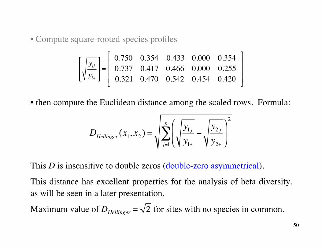
• Compute square-rooted species profiles
• then compute the Euclidean distance among the scaled rows. Formula:
This D is insensitive to double zeros (double-zero asymmetrical).
This distance has excellent properties for the analysis of beta diversity, as will be seen in a later presentation.
Maximum value of DHellinger = for sites with no species in common.
DHellinger (x1, x2 ) =y1 jy1+
−y2 jy2+
⎛
⎝⎜⎜
⎞
⎠⎟⎟
2
j=1
p
∑
yijyi+
⎡
⎣⎢⎢
⎤
⎦⎥⎥=
0.750 0.354 0.433 0.000 0.3540.737 0.417 0.466 0.000 0.2550.321 0.470 0.542 0.454 0.420
⎡
⎣
⎢⎢⎢
⎤
⎦
⎥⎥⎥
2
50
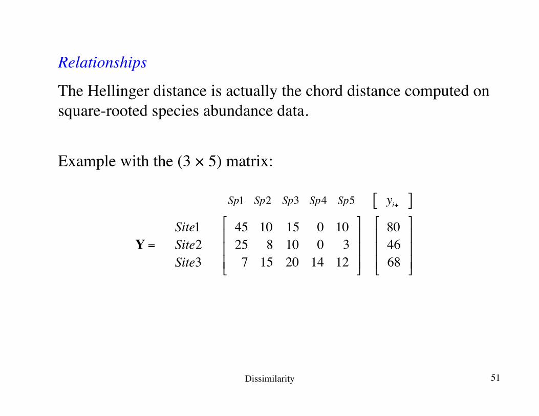
Relationships
The Hellinger distance is actually the chord distance computed on square-rooted species abundance data.
Example with the (3 × 5) matrix:
Sp1 Sp2 Sp3 Sp4 Sp5 yi+ [ ]
Y =Site1Site2Site3
45 10 15 0 1025 8 10 0 37 15 20 14 12
⎡
⎣
⎢⎢⎢
⎤
⎦
⎥⎥⎥
804668
⎡
⎣
⎢⎢⎢
⎤
⎦
⎥⎥⎥
Dissimilarity 51
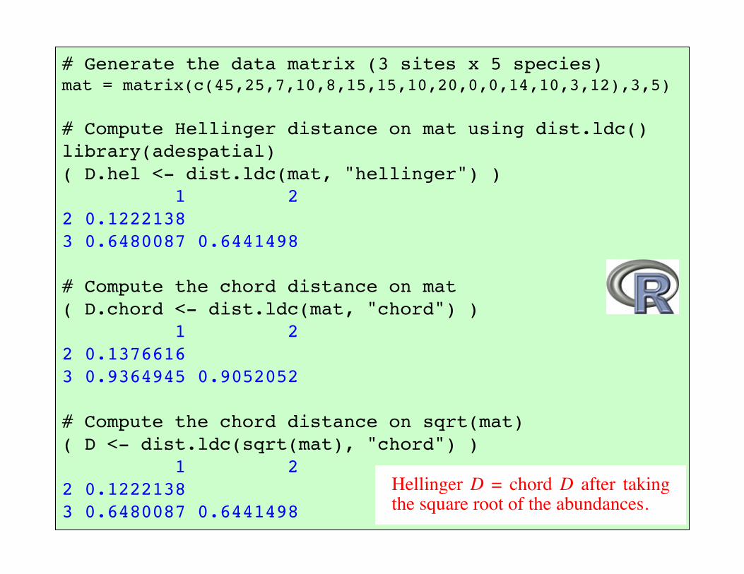
# Generate the data matrix (3 sites x 5 species)mat = matrix(c(45,25,7,10,8,15,15,10,20,0,0,14,10,3,12),3,5)
# Compute Hellinger distance on mat using dist.ldc()library(adespatial)( D.hel <- dist.ldc(mat, "hellinger") ) 1 22 0.1222138 3 0.6480087 0.6441498
# Compute the chord distance on mat( D.chord <- dist.ldc(mat, "chord") ) 1 22 0.1376616 3 0.9364945 0.9052052
# Compute the chord distance on sqrt(mat)( D <- dist.ldc(sqrt(mat), "chord") ) 1 22 0.1222138 3 0.6480087 0.6441498
Hellinger D = chord D after taking the square root of the abundances.
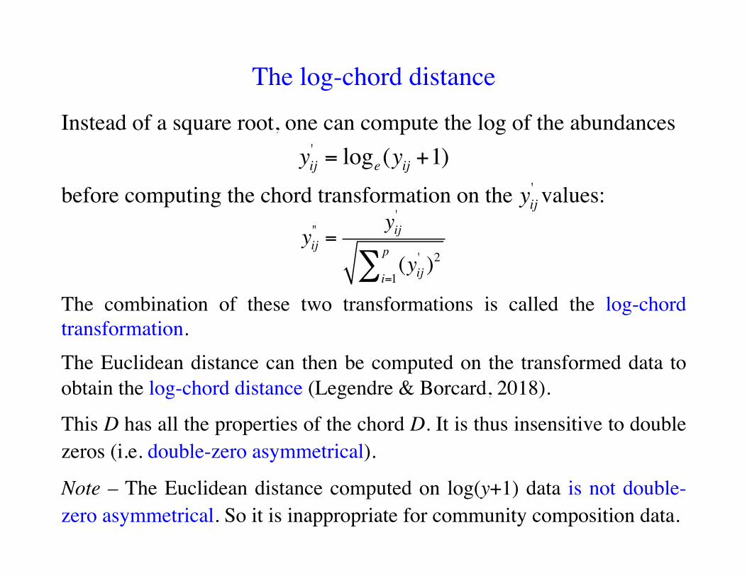
The log-chord distance
Instead of a square root, one can compute the log of the abundances
before computing the chord transformation on the values:
The combination of these two transformations is called the log-chord transformation.The Euclidean distance can then be computed on the transformed data to obtain the log-chord distance (Legendre & Borcard, 2018).
This D has all the properties of the chord D. It is thus insensitive to double zeros (i.e. double-zero asymmetrical).
Note – The Euclidean distance computed on log(y+1) data is not double-zero asymmetrical. So it is inappropriate for community composition data.
yij' = loge(yij +1)
yij" =
yij'
(yij' )2
i=1
p∑
yij'
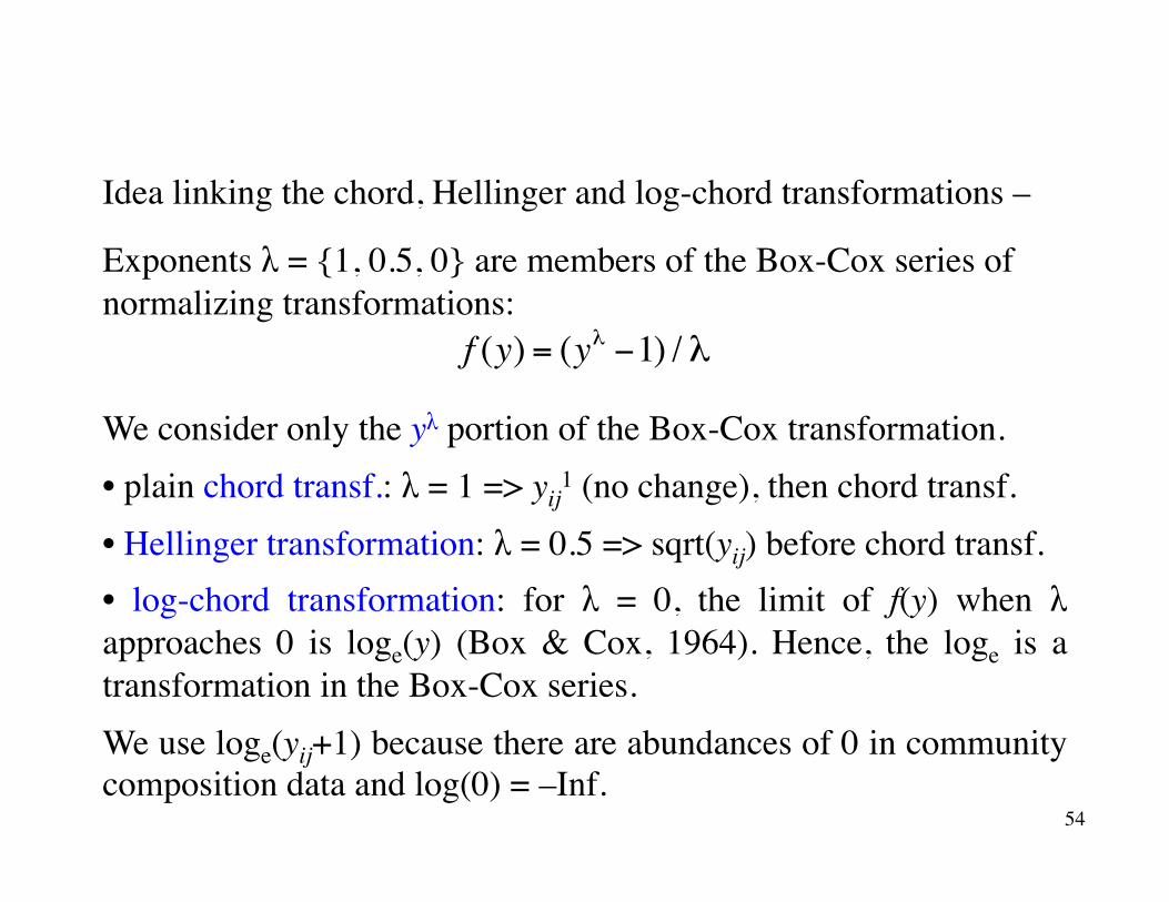
Idea linking the chord, Hellinger and log-chord transformations –
Exponents λ = {1, 0.5, 0} are members of the Box-Cox series of normalizing transformations:
We consider only the yλ portion of the Box-Cox transformation.• plain chord transf.: λ = 1 => yij
1 (no change), then chord transf.• Hellinger transformation: λ = 0.5 => sqrt(yij) before chord transf. • log-chord transformation: for λ = 0, the limit of f(y) when λ approaches 0 is loge(y) (Box & Cox, 1964). Hence, the loge is a transformation in the Box-Cox series.We use loge(yij+1) because there are abundances of 0 in community composition data and log(0) = –Inf.
f (y) = (yλ −1) / λ
54
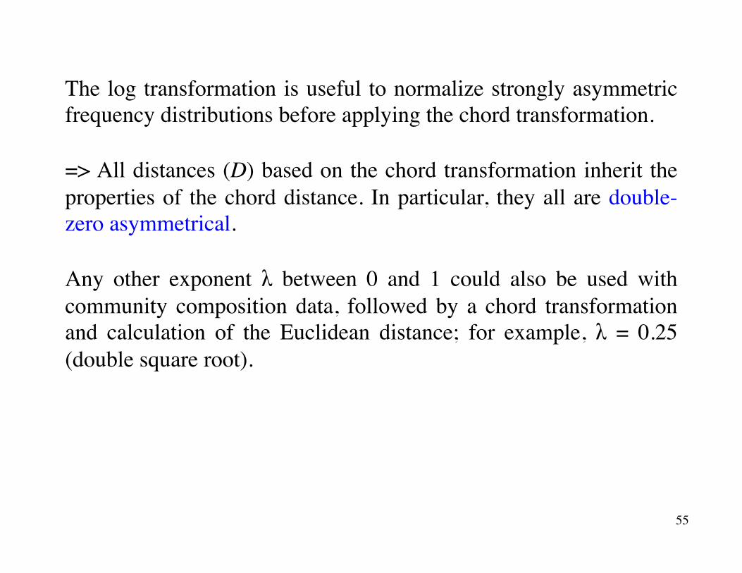
The log transformation is useful to normalize strongly asymmetric frequency distributions before applying the chord transformation.
=> All distances (D) based on the chord transformation inherit the properties of the chord distance. In particular, they all are double-zero asymmetrical.
Any other exponent λ between 0 and 1 could also be used with community composition data, followed by a chord transformation and calculation of the Euclidean distance; for example, λ = 0.25 (double square root).
55
The chi-square distance is an important coefficient. It is the distance preserved in correspondence analysis (CA).
The chi-square distance can only be computed on data that are non-negative (i.e. ≥ 0), frequency-like1, and dimensionally homogeneous.
1 Examples: community composition or biomass data; monetary units (e.g. $, £, €, ¥).
The chi-square distance
56
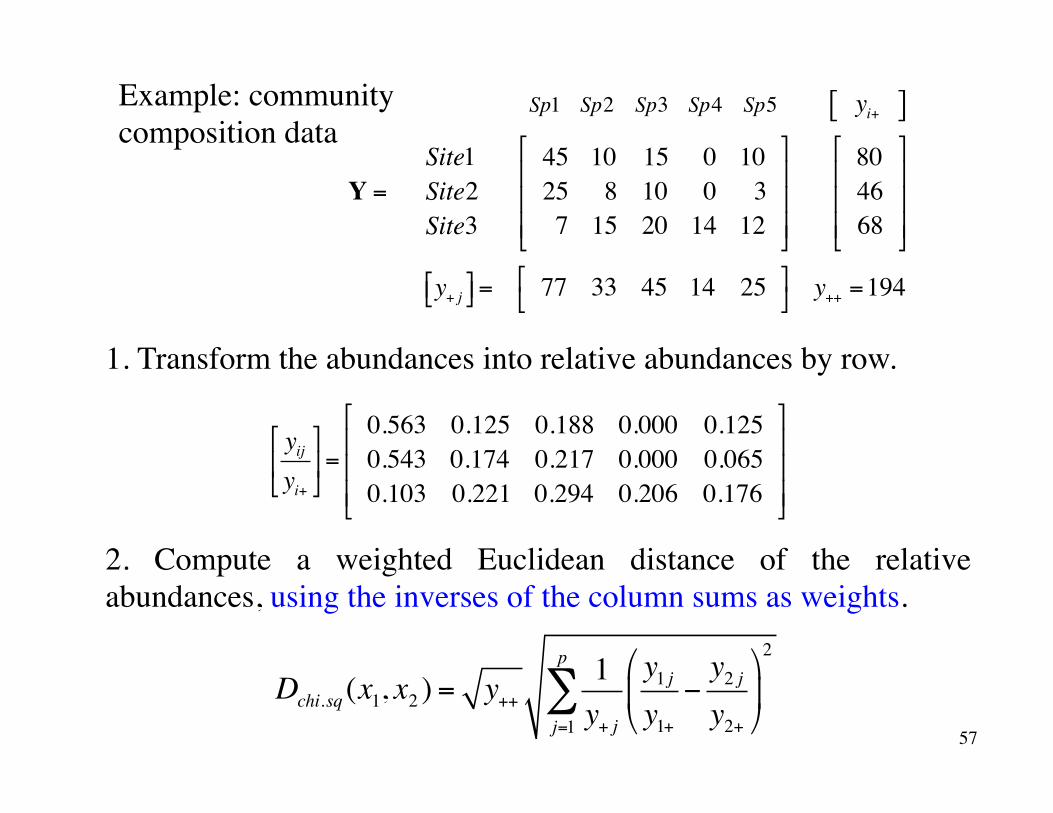
Example: community composition data
Sp1 Sp2 Sp3 Sp4 Sp5 yi+ [ ]
Y =Site1Site2Site3
45 10 15 0 1025 8 10 0 37 15 20 14 12
⎡
⎣
⎢⎢⎢
⎤
⎦
⎥⎥⎥
804668
⎡
⎣
⎢⎢⎢
⎤
⎦
⎥⎥⎥
y+ j⎡⎣ ⎤⎦= 77 33 45 14 25⎡⎣
⎤⎦ y++ =194
1. Transform the abundances into relative abundances by row.
2. Compute a weighted Euclidean distance of the relative abundances, using the inverses of the column sums as weights.
yijyi+
⎡
⎣⎢
⎤
⎦⎥=
0.563 0.125 0.188 0.000 0.1250.543 0.174 0.217 0.000 0.0650.103 0.221 0.294 0.206 0.176
⎡
⎣
⎢⎢⎢
⎤
⎦
⎥⎥⎥
Dchi.sq (x1, x2 ) = y++1y+ j
y1 jy1+
−y2 jy2+
⎛
⎝⎜
⎞
⎠⎟
2
j=1
p
∑57
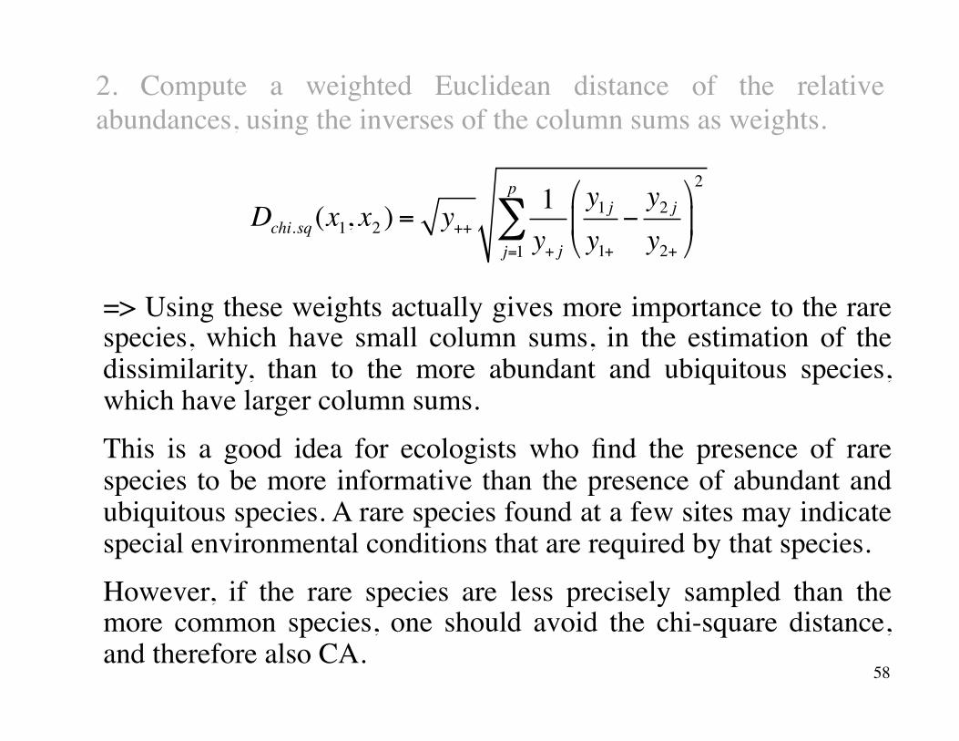
2. Compute a weighted Euclidean distance of the relative abundances, using the inverses of the column sums as weights.
Dchi.sq (x1, x2 ) = y++1y+ j
y1 jy1+
−y2 jy2+
⎛
⎝⎜
⎞
⎠⎟
2
j=1
p
∑
=> Using these weights actually gives more importance to the rare species, which have small column sums, in the estimation of the dissimilarity, than to the more abundant and ubiquitous species, which have larger column sums.
This is a good idea for ecologists who find the presence of rare species to be more informative than the presence of abundant and ubiquitous species. A rare species found at a few sites may indicate special environmental conditions that are required by that species.
However, if the rare species are less precisely sampled than the more common species, one should avoid the chi-square distance, and therefore also CA.
58
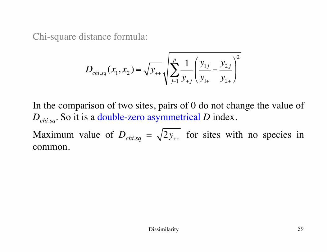
Chi-square distance formula:
Dchi.sq (x1, x2 ) = y++1y+ j
y1 jy1+
−y2 jy2+
⎛
⎝⎜
⎞
⎠⎟
2
j=1
p
∑
In the comparison of two sites, pairs of 0 do not change the value of Dchi.sq. So it is a double-zero asymmetrical D index.
Maximum value of Dchi.sq = for sites with no species in common.
2y++
Dissimilarity 59
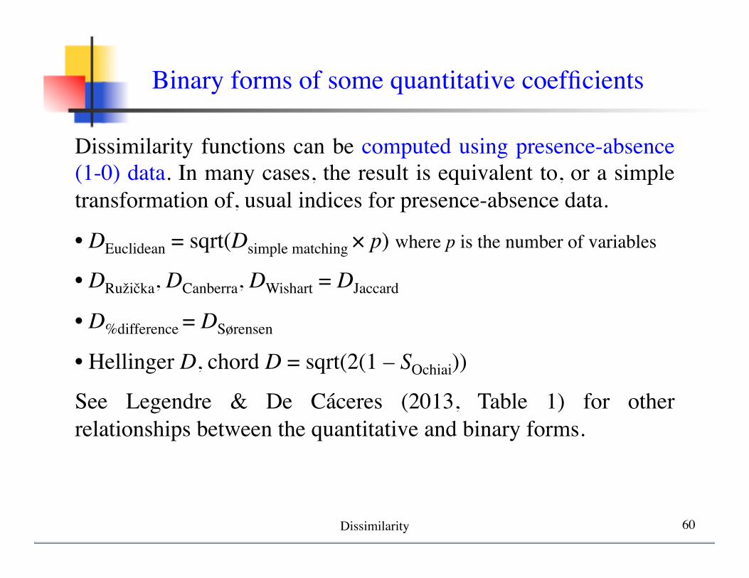
Dissimilarity functions can be computed using presence-absence (1-0) data. In many cases, the result is equivalent to, or a simple transformation of, usual indices for presence-absence data.
• DEuclidean = sqrt(Dsimple matching × p) where p is the number of variables
• DRužička, DCanberra, DWishart = DJaccard
• D%difference = DSørensen
• Hellinger D, chord D = sqrt(2(1 – SOchiai))
See Legendre & De Cáceres (2013, Table 1) for other relationships between the quantitative and binary forms.
Binary forms of some quantitative coefficients
Dissimilarity 60
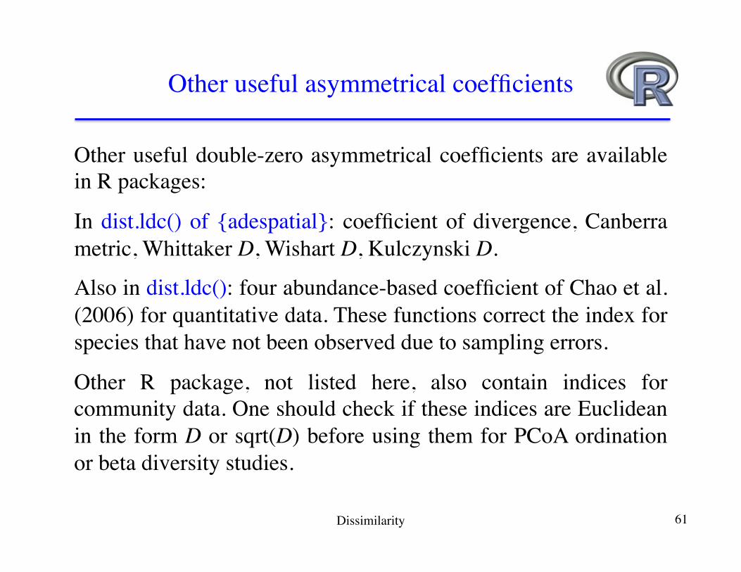
Other useful double-zero asymmetrical coefficients are available in R packages:
In dist.ldc() of {adespatial}: coefficient of divergence, Canberra metric, Whittaker D, Wishart D, Kulczynski D.
Also in dist.ldc(): four abundance-based coefficient of Chao et al. (2006) for quantitative data. These functions correct the index for species that have not been observed due to sampling errors.
Other R package, not listed here, also contain indices for community data. One should check if these indices are Euclidean in the form D or sqrt(D) before using them for PCoA ordination or beta diversity studies.
Other useful asymmetrical coefficients
Dissimilarity 61
Compute asymmetrical D indices for community composition data
as follows:
• data transformation
• followed by calculation of the Euclidean distance,
as shown in the section on asymmetrical indices for quantitative community composition data.
Computing D through data transformations
Dissimilarity 62
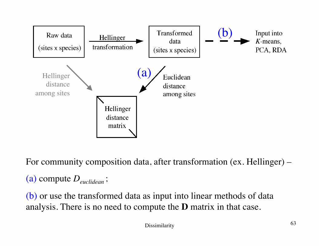
For community composition data, after transformation (ex. Hellinger) –
(a) compute Deuclidean ;
(b) or use the transformed data as input into linear methods of data analysis. There is no need to compute the D matrix in that case.
Dissimilarity
Hellinger distance
among sites
(a)
(b)
63
Ordination in reduced space
3. Pre-transformation of species data: illustrationThe species abundance paradox (Orlóci, 1978)
Transformations for community composition data 329
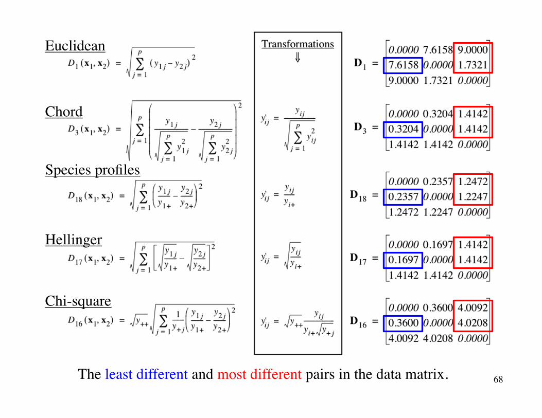
Figure 7.8 Species abundance paradox data, modified from Orlóci (1978). The paradox is that the
Euclidean distance between sites 2 and 3, which have no species in common, is smaller than that
between sites 1 and 2 which share species 2 and 3. This results in an incorrect assessment of the
ecological relationships among sites. With the other coefficients in this figure, which are
asymmetrical, the distance between sites 2 and 3 is larger than that between sites 1 and 2, and
the distance between sites 1 and 3 is the same as between sites 2 and 3, or very nearly so.
Distance matrix D15 (not shown) is equal to D16/ = D16/ .y++
15
Chord
Species profiles
Hellinger
Chi-square
Euclidean
Dissimilarity 64
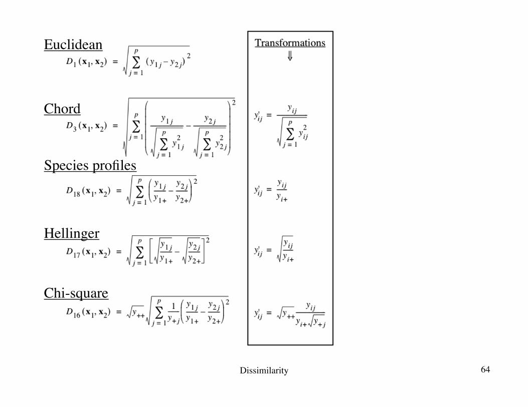
The previous slide shows …… that the chord, species profile, Hellinger and chi-square transformations, followed by calculation of the Euclidean distance, produce the same-name dissimilarity indices, which are
• double-zero asymmetrical, • metric • and Euclidean.
The log-chord transformation, followed by the Euclidean distance, produces the log-chord distance, which also has these properties.
Dissimilarity 65
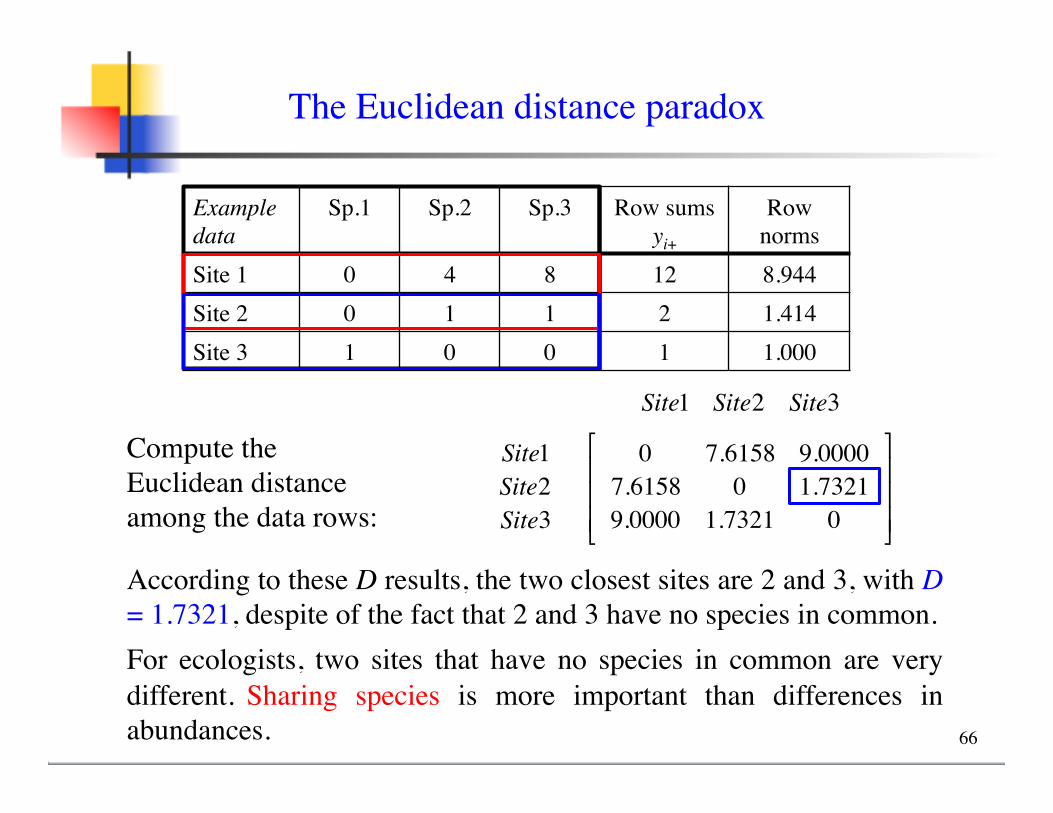
The Euclidean distance paradox
Example data
Sp.1 Sp.2 Sp.3 Row sumsyi+
Row norms
Site 1 0 4 8 12 8.944Site 2 0 1 1 2 1.414Site 3 1 0 0 1 1.000
Compute the Euclidean distance among the data rows:
Site1 Site2 Site3
Site1Site2Site3
0 7.6158 9.00007.6158 0 1.73219.0000 1.7321 0
⎡
⎣
⎢⎢⎢
⎤
⎦
⎥⎥⎥
According to these D results, the two closest sites are 2 and 3, with D = 1.7321, despite of the fact that 2 and 3 have no species in common.For ecologists, two sites that have no species in common are very different. Sharing species is more important than differences in abundances. 66
Site1 Site2 Site3
Site1Site2Site3
0 7.6158 9.00007.6158 0 1.73219.0000 1.7321 0
⎡
⎣
⎢⎢⎢
⎤
⎦
⎥⎥⎥
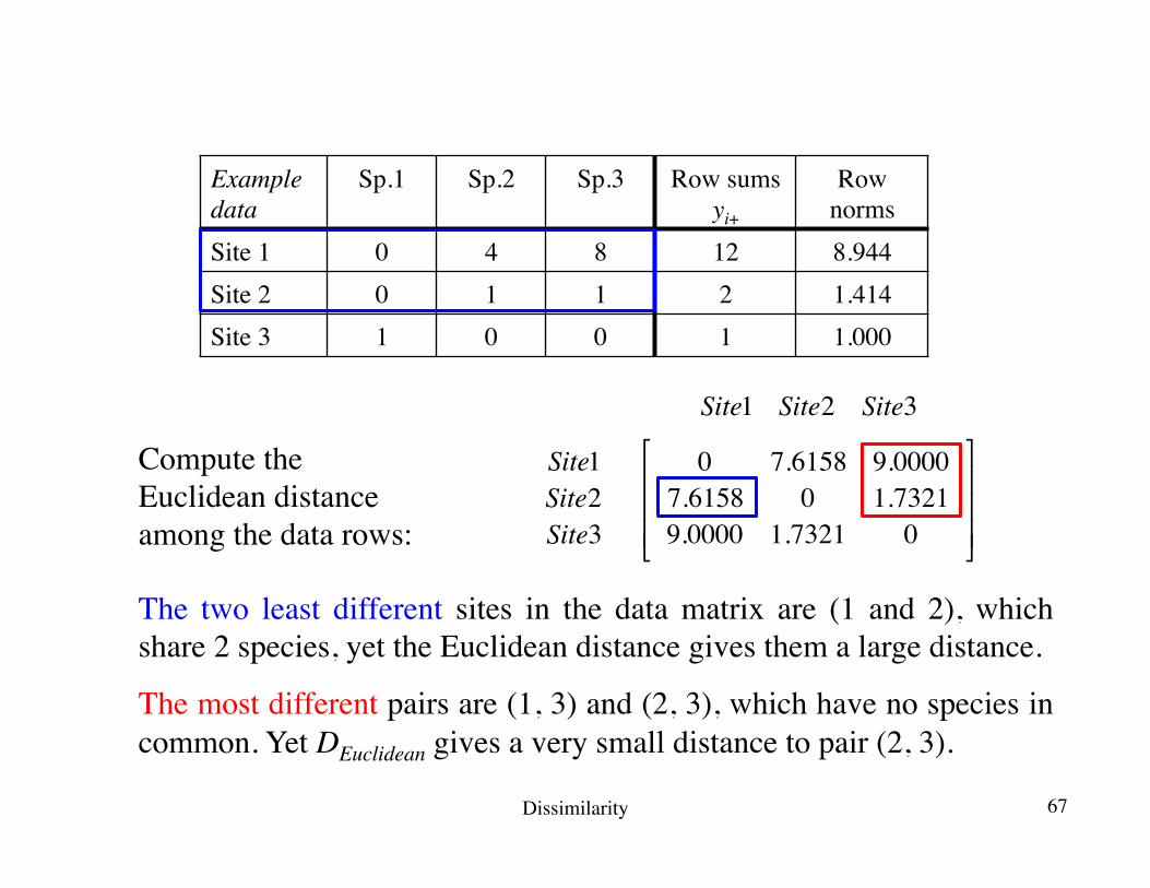
The two least different sites in the data matrix are (1 and 2), which share 2 species, yet the Euclidean distance gives them a large distance.
The most different pairs are (1, 3) and (2, 3), which have no species in common. Yet DEuclidean gives a very small distance to pair (2, 3).
Compute the Euclidean distance among the data rows:
Example data
Sp.1 Sp.2 Sp.3 Row sumsyi+
Row norms
Site 1 0 4 8 12 8.944Site 2 0 1 1 2 1.414Site 3 1 0 0 1 1.000
Dissimilarity 67
Ordination in reduced space
3. Pre-transformation of species data: illustrationThe species abundance paradox (Orlóci, 1978)
Transformations for community composition data 329
Figure 7.8 Species abundance paradox data, modified from Orlóci (1978). The paradox is that the
Euclidean distance between sites 2 and 3, which have no species in common, is smaller than that
between sites 1 and 2 which share species 2 and 3. This results in an incorrect assessment of the
ecological relationships among sites. With the other coefficients in this figure, which are
asymmetrical, the distance between sites 2 and 3 is larger than that between sites 1 and 2, and
the distance between sites 1 and 3 is the same as between sites 2 and 3, or very nearly so.
Distance matrix D15 (not shown) is equal to D16/ = D16/ .y++
15
Chord
Species profiles
Hellinger
Chi-square
Euclidean
The least different and most different pairs in the data matrix. 68
The previous slide shows …… that the Euclidean distance can give a small D value to a pair of sites (2, 3) that have no species in common, indicating that they are highly similar.Contrary to that, the chord, species profile, Hellinger and chi-square distances produce smaller D values for the pair of sites (1, 2) that contains the same species than for pairs of sites where different species assemblages are found.
Dissimilarity 69
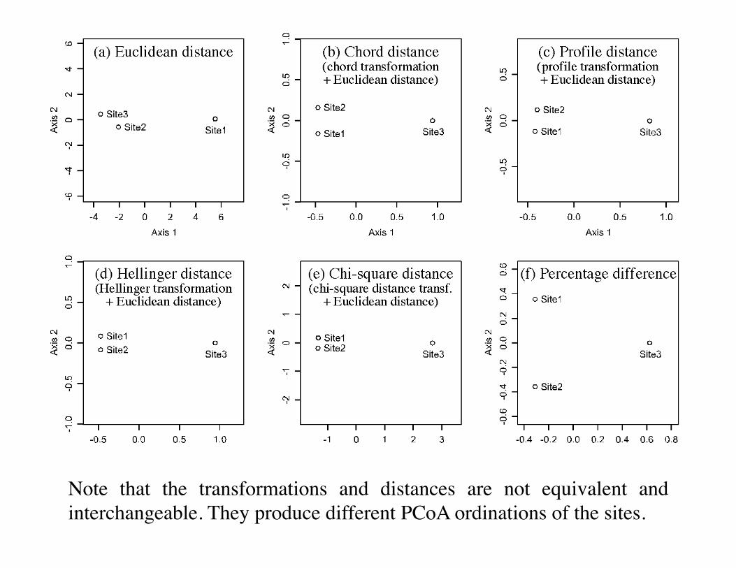
Note that the transformations and distances are not equivalent and interchangeable. They produce different PCoA ordinations of the sites.
Data transformations in
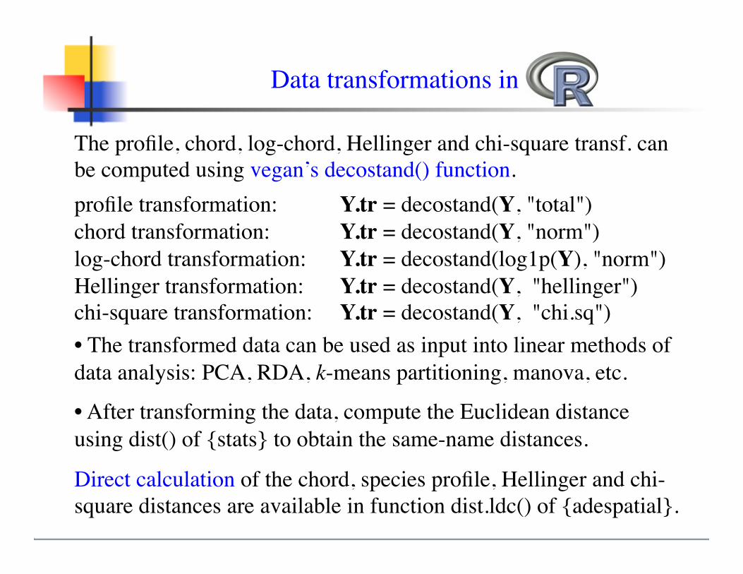
The profile, chord, log-chord, Hellinger and chi-square transf. can be computed using vegan’s decostand() function.profile transformation: Y.tr = decostand(Y, "total")chord transformation: Y.tr = decostand(Y, "norm")log-chord transformation: Y.tr = decostand(log1p(Y), "norm")Hellinger transformation: Y.tr = decostand(Y, "hellinger")chi-square transformation: Y.tr = decostand(Y, "chi.sq")• The transformed data can be used as input into linear methods of data analysis: PCA, RDA, k-means partitioning, manova, etc.
• After transforming the data, compute the Euclidean distance using dist() of {stats} to obtain the same-name distances.
Direct calculation of the chord, species profile, Hellinger and chi-square distances are available in function dist.ldc() of {adespatial}.
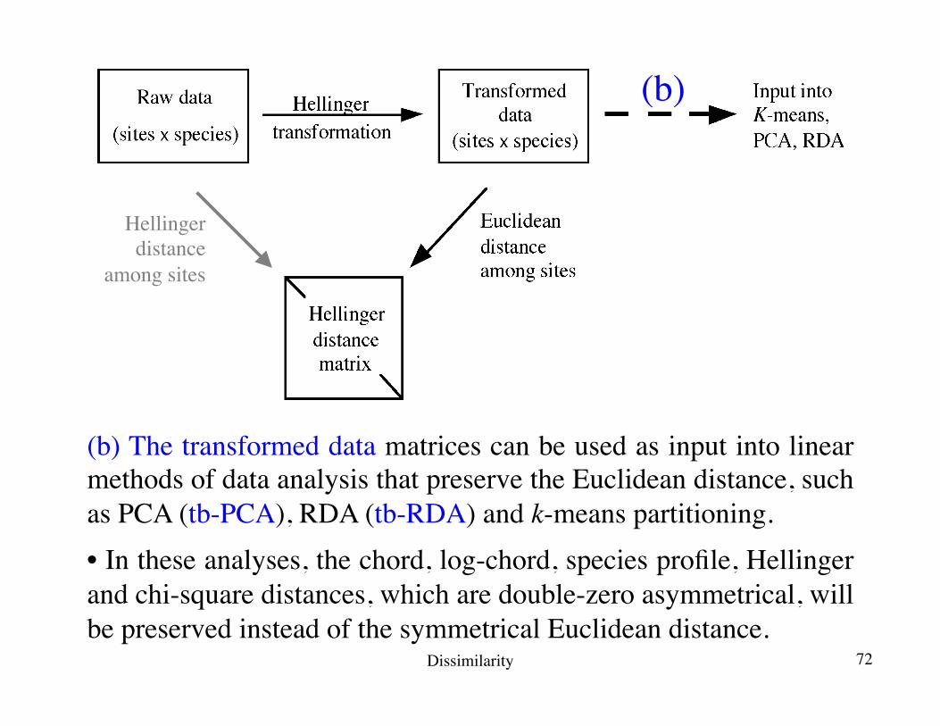
(b) The transformed data matrices can be used as input into linear methods of data analysis that preserve the Euclidean distance, such as PCA (tb-PCA), RDA (tb-RDA) and k-means partitioning.• In these analyses, the chord, log-chord, species profile, Hellinger and chi-square distances, which are double-zero asymmetrical, will be preserved instead of the symmetrical Euclidean distance.
Hellinger distance
among sites
(b)
Dissimilarity 72
ReferencesBox, G. E. P. & D. R. Cox. 1964. An analysis of transformations. J. Roy. Statist. Soc. Ser. B
26: 211–243.Borcard, D., F. Gillet & P. Legendre. 2018. Numerical ecology with R, 2nd edition. Use R! series,
Springer International Publishing, New York.Bray, R. J. & J. T. Curtis. 1957. An ordination of the upland forest communities of southern
Wisconsin. Ecological Monographs 27: 325–349.Chao, A., R. L. Chazdon, R. K. Colwell & T. J. Shen. 2006. Abundance-based similarity indices
and their estimation when there are unseen species in samples. Biometrics 62: 361–371. Gower, J. C. 1971. A general coefficient of similarity and some of its properties. Biometrics 27:
857-871.Legendre, P. & D. Borcard. 2018. Box-Cox-chord transformations for community composition
data prior to beta diversity analysis. Ecography 41: 1–5.Legendre, P. & M. De Cáceres. 2013. Beta diversity as the variance of community data:
dissimilarity coefficients and partitioning. Ecology Letters 16: 951-963.Legendre, P. & L. Legendre. 2012. Numerical ecology, 3rd English edition. Elsevier Science BV,
Amsterdam. xvi + 990 pp. ISBN-13: 978-0444538680. Odum, E. P. 1950. Bird populations of the Highlands (North Carolina) Plateau in relation to plant
succession and avian invasion. Ecology 31: 587–605.Whittaker, R. H. 1952. A study of summer foliage insect communities in the Great Smoky
Mountains. Ecological Monographs 22: 1–44.Whittaker, R. H. 1972. Evolution and measurement of species diversity. Taxon 21: 213-251. 73

End of the presentation


![arXiv:1901.05498v2 [cs.LG] 20 Jan 2019MuSAE Lab INRS-EMT Université du Québec Montréal, Canada Jocelyn Faubert Faubert Lab Université de Montréal Montréal,Canada ABSTRACT Context](https://img.pdfslide.us/doc/110x75/6022f103e96d80312222c55b/arxiv190105498v2-cslg-20-jan-2019-musae-lab-inrs-emt-universit-du-qubec.jpg)