UNIVERSIDAD AUT“NOMA DE MADRID PROYECTO FIN DE CARRERA Software quality studies

UNIVERSIDAD AUTÓNOMA DE MADRIDESCUELA POLITÉCNICA SUPERIOR

PROYECTO FIN DE CARRERA

Software quality studies using analyticalmetric analysis

Cecilia Rodríguez MartínezApril 2013

Software quality studies using analytical metricanalysis

Cecilia Rodríguez Martínez

3 April 2013

Master Thesis

KTH Academic Supervisor: Gerald Q. Maguire Jr.Presenter: Eloy Anguiano

Stockholm,Sweden

AbstractToday engineering companies expend a large amount of resources on the detection and

correction of the bugs (defects) in their software. These bugs are usually due to errors andmistakes made by programmers while writing the code or writing the specifications. No toolis able to detect all of these bugs. Some of these bugs remain undetected despite testing ofthe code. For these reasons, many researchers have tried to find indicators in the software’ssource codes that can be used to predict the presence of bugs.

Every bug in the source code is a potentially failure of the program to perform asexpected. Therefore, programs are tested with many different cases in an attempt to coverall the possible paths through the program to detect all of these bugs. Early predictionof bugs informs the programmers about the location of the bugs in the code. Thus,programmers can more carefully test the more error prone files, and thus save a lot oftime by not testing error free files.

This thesis project created a tool that is able to predict error prone source codewritten in C++. In order to achieve this, we have utilized one predictor which has beenextremely well studied: software metrics. Many studies have demonstrated that thereis a relationship between software metrics and the presence of bugs. In this project aNeuro-Fuzzy hybrid model based on Fuzzy c-means and Radial Basis Neural Networkhas been used. The efficiency of the model has been tested in a software project atEricsson. Testing of this model proved that the program does not achieve high accuracydue to the lack of independent samples in the data set. However, experiments did showthat classification models provide better predictions than regression models. The thesisconcluded by suggesting future work that could improve the performance of this program.

Keywords: Bugs, Fuzzy c-means, Neuro-fuzzy hybrid model, Radial basis functionneural network, Software metrics

SammanfattningIdag spenderar ingenjörsföretag en stor mängd resurser på att upptäcka och korrigera

buggar (fel) i sin mjukvara. Det är oftast programmerare som inför dessa buggar på grund avfel och misstag som uppkommer när de skriver koden eller specifikationerna. Inget verktygkan detektera alla dessa buggar. Några av buggarna förblir oupptäckta trots testning avkoden. Av dessa skäl har många forskare försökt hitta indikatorer i programvarans källkodsom kan användas för att förutsäga förekomsten av buggar.

Varje fel i källkoden är ett potentiellt misslyckande som gör att applikationen intefungerar som förväntat. För att hitta buggarna testas koden med många olika testfall föratt försöka täcka alla möjliga kombinationer och fall. Förutsägelse av buggar informerarprogrammerarna om var i koden buggarna finns. Således kan programmerarna mer noggranttesta felbenägna filer och därmed spara mycket tid genom att inte behöva testa felfria filer.

Detta examensarbete har skapat ett verktyg som kan förutsäga felbenägen källkodskriven i C ++. För att uppnå detta har vi utnyttjat en välkänd metod som heterSoftware Metrics. Många studier har visat att det finns ett samband mellan SoftwareMetrics och förekomsten av buggar. I detta projekt har en Neuro-Fuzzy hybridmodellbaserad på Fuzzy c-means och Radial Basis Neural Network använts. Effektiviteten avmodellen har testats i ett mjukvaruprojekt på Ericsson. Testning av denna modell visadeatt programmet inte Uppnå hög noggrannhet på grund av bristen av oberoende urval idatauppsättningen. Men gjordt experiment visade att klassificering modeller ger bättreförutsägelser än regressionsmodeller. Exjobbet avslutade genom att föreslå framtida arbetetsom skulle kunna förbättra detta program.

Keywords: Buggar, Fuzzy c-medel, Neuro-Fuzzy hybridmodell, Radial basis funktionneurala nätverk, programvarastatistik

ResumenActualmente las empresas de ingeniería derivan una gran cantidad de recursos a la de-

tección y corrección de errores en sus códigos software. Estos errores se deben generalmente alos errores cometidos por los desarrolladores cuando escriben el código o sus especificaciones.No hay ninguna herramienta capaz de detectar todos estos errores y algunos de ellos pasandesapercibidos tras el proceso de pruebas. Por esta razón, numerosas investigaciones hanintentado encontrar indicadores en los códigos fuente del software que puedan ser utilizadospara detectar la presencia de errores.

Cada error en un código fuente es un error potencial en el funcionamiento del programa,por ello los programas son sometidos a exhaustivas pruebas que cubren (o intentan cubrir)todos los posibles caminos del programa para detectar todos sus errores. La tempranalocalización de errores informa a los programadores dedicados a la realización de estaspruebas sobre la ubicación de estos errores en el código. Así, los programadores puedenprobar con más cuidado los archivos más propensos a tener errores dejando a un lado losarchivos libres de error.

En este proyecto se ha creado una herramienta capaz de predecir código softwarepropenso a errores escrito en C++. Para ello, en este proyecto se ha utilizado un indicadorque ha sido cuidadosamente estudiado y ha demostrado su relación con la presencia deerrores: las métricas del software. En este proyecto un modelo híbrido neuro-disfuso basadoen Fuzzy c-means y en redes neuronales de función de base radial ha sido utilizado. Laeficacia de este modelo ha sido probada en un proyecto software de Ericsson. Como resultadose ha comprobado que el modelo no alcanza una alta precisión debido a la falta de muestrasindependientes en el conjunto de datos y los experimentos han mostrado que los modelos declasificación proporcionan mejores predicciones que los modelos de regresión. El proyectoconcluye sugiriendo trabajo que mejoraría el funcionamiento del programa en el futuro.

Keywords: Error, Fuzzy c-means, modelo híbrido neuro-difuso, Red neuronal defunción de base radial, métricas del software

Acknowledgements

First of all, I would like to thank my Ericsson’s industrial supervisor Hamidreza Yazdanifor trusting me and give me this great opportunity. I am also grateful to Gerald Maguirefor being my examiner and for being always available to help, and to Eloy Anguiano forbeing my presenter making this possible.

I want to thank my friends from my home university because they pushed me heremaking my life amazing at the EPS, specially to Guillermo Gálvez for being the best friendand colleague during these five years. You guys brought me here!

I want to dedicate my PFC to Mónica Estevez and my girls for being always proud ofme and being always there when I need it. I also want to acknowledge all my friends fromTres Cantos for supporting me and share their lives with me even in the distance. Yousimply make me happy.

I really want to thank my brother, Juan Rodríguez, for helping me and encouraging meevery time I doubt, and to my family for helping me to achieve all my goals in my life.

I want to make a special mention to Jesus Paredes for his continuous support andconfidence, to Nacho Mulas for listening to me every time I need it, to Alberto Fernandez,and to all the friends I met in Stockholm, you made warm this cold country!

Finally I also want to thank the people from COM for making me feel one more of theteam, specially to Belén Valcarce-Pérez, Péter Dimitrov and the foosball team; I promise"I will do something".

Contents

Contents X

List of Figures XIII

List of Tables XIV

List of Acronyms XV

1 Introduction 11.1. Problem Statement . . . . . . . . . . . . . . . . . . . . . . . . . . . . 21.2. Goals . . . . . . . . . . . . . . . . . . . . . . . . . . . . . . . . . . . 31.3. Scope . . . . . . . . . . . . . . . . . . . . . . . . . . . . . . . . . . . 31.4. Target Audience . . . . . . . . . . . . . . . . . . . . . . . . . . . . . 41.5. Methodology . . . . . . . . . . . . . . . . . . . . . . . . . . . . . . . 41.6. Structure . . . . . . . . . . . . . . . . . . . . . . . . . . . . . . . . . 5

2 Background 72.1. Software Metrics . . . . . . . . . . . . . . . . . . . . . . . . . . . . . 7

2.1.1. Basic Concepts . . . . . . . . . . . . . . . . . . . . . . . . . . 82.1.2. Definition of Metrics . . . . . . . . . . . . . . . . . . . . . . . 82.1.3. Software metrics measurement programs . . . . . . . . . . . . 12

2.2. Regression Models . . . . . . . . . . . . . . . . . . . . . . . . . . . . 132.2.1. Artificial Neural Networks . . . . . . . . . . . . . . . . . . . 152.2.2. Clustering . . . . . . . . . . . . . . . . . . . . . . . . . . . . . 19

3 Analysis 253.0.3. Specification . . . . . . . . . . . . . . . . . . . . . . . . . . . 253.0.4. Selection of the model . . . . . . . . . . . . . . . . . . . . . . 25

4 Model implementation 274.1. Hybrid topology . . . . . . . . . . . . . . . . . . . . . . . . . . . . . 274.2. Extraction of metrics and bugs . . . . . . . . . . . . . . . . . . . . . 29

4.2.1. Extracting the metrics . . . . . . . . . . . . . . . . . . . . . . 304.2.2. Extracting information about bugs . . . . . . . . . . . . . . . 32

x

4.3. FCM Clustering . . . . . . . . . . . . . . . . . . . . . . . . . . . . . 324.4. RBFNN . . . . . . . . . . . . . . . . . . . . . . . . . . . . . . . . . . 344.5. Experiments and results . . . . . . . . . . . . . . . . . . . . . . . . . 35

5 Design of the tool 415.1. Analysis of the tool . . . . . . . . . . . . . . . . . . . . . . . . . . . . 41

6 Conclusion 43

7 Future work 457.1. Model improvements . . . . . . . . . . . . . . . . . . . . . . . . . . . 457.2. Tool improvements . . . . . . . . . . . . . . . . . . . . . . . . . . . . 46

8 Required reflections 47

Bibliography 49

A Sinopsis of the tool 53

B Requirements of the tool 55

C Introducción 57C.1. Descripción del problema . . . . . . . . . . . . . . . . . . . . . . . . 58C.2. Objetivos . . . . . . . . . . . . . . . . . . . . . . . . . . . . . . . . . 58C.3. Estructura . . . . . . . . . . . . . . . . . . . . . . . . . . . . . . . . . 59

D Conclusiones 61

E Presupuesto 63

F Pliego de condiciones 65

List of Figures

1.1. A software development process according to the waterfall model . . . . 2

2.1. An example of an artificial neural network . . . . . . . . . . . . . . . . 152.2. A neuron of a generic artificial neural network . . . . . . . . . . . . . . 162.3. A neuron of a backpropagation neural network . . . . . . . . . . . . . . 172.4. Hard partitioning over a data set . . . . . . . . . . . . . . . . . . . . . . 202.5. Soft partitioning over a data set . . . . . . . . . . . . . . . . . . . . . . 202.6. Results of Gustafson-Kessel Algorithm over a data set . . . . . . . . . . 22

4.1. Example of an hybrid topology with 5 clusters . . . . . . . . . . . . . . 284.2. ROC curve of the regression model 10-8-1 . . . . . . . . . . . . . . . . . 384.3. ROC curve of the classification model 10-10-1 . . . . . . . . . . . . . . . 39

xiii

List of Tables

2.1. Object Oriented Metrics . . . . . . . . . . . . . . . . . . . . . . . . . . . 92.2. Object Oriented CK Metrics . . . . . . . . . . . . . . . . . . . . . . . . 102.3. Object Oriented BUGFIXES Metric . . . . . . . . . . . . . . . . . . . . 122.4. Comparison between programs by the metrics they compute . . . . . . . 132.5. Comparison between programs based upon their languages and license . 13

4.1. Confusion Matrix . . . . . . . . . . . . . . . . . . . . . . . . . . . . . . . 284.2. CCCC metrics’ definition . . . . . . . . . . . . . . . . . . . . . . . . . . 314.3. Output functions of the neurons of the network . . . . . . . . . . . . . . 344.4. Cluster validity indexes . . . . . . . . . . . . . . . . . . . . . . . . . . . 364.5. Quality validity 10-4-1 . . . . . . . . . . . . . . . . . . . . . . . . . . . . 364.6. Quality validity 8-2-1 . . . . . . . . . . . . . . . . . . . . . . . . . . . . . 374.7. Quality validity . . . . . . . . . . . . . . . . . . . . . . . . . . . . . . . . 38

xiv

List of Acronyms

ANN Artificial Neural Network

BPNN Back Propagation Neural Network

CBO Coupling Between Objects

CCCC C and C++ Code Counter

CK Chidember and Kemerer

CS Compact-Separate

DIT Depth of Inheritance Tree

FCM Fuzzy c-means

FLD Fisher’s Linear Discriminant

FS Fukuyama.sugeno

GK Gustafson-Kessel algorithm

HTML HyperText Markup Language

IFc Information Flow complexity

JMT Java Measurement Tool

LCOM Lack of COhesion in Mthods

LOC Lines Of Code

NN Neural network

NOA Number Of Attributes

NOC Number Of Children

NOM Number Of Modules

OO Object Oriented

PC Partition.coefficient

xv

PE Partition.entropy

PHP Hypertext Preprocessor

PL Procedural language

RBF Radial Basis Function

RBFNN Radial Basis Function Neural Network

RFC Response For a Class

RMS Root Mean Square

ROC Receiving Operating Characteristic

RSM Resource Standard Metrics

SNNS Stuttgart Neural Network Simulator

SQL Structured Query Language

WMC Weighted Methods per Class

XB Xie.beni

XML Extendible Markup Language

Chapter 1

Introduction

These days, the telecommunication industry is an open market accessible to allenterprises. In a market where many companies compete to be the market leaderscompanies need to offer a high level of quality and reliability in their products inorder to maintain their market position. Delivering high quality and highly reliablesoftware is a mandatory goal for software development companies, as this reducesthe amount of resources needed to support the software after it has been deliveredand this quality helps the firm to gain a larger portion of the market. Therefore,managers involved in the development and maintenance of software now focus onenhancing their software development process [10].

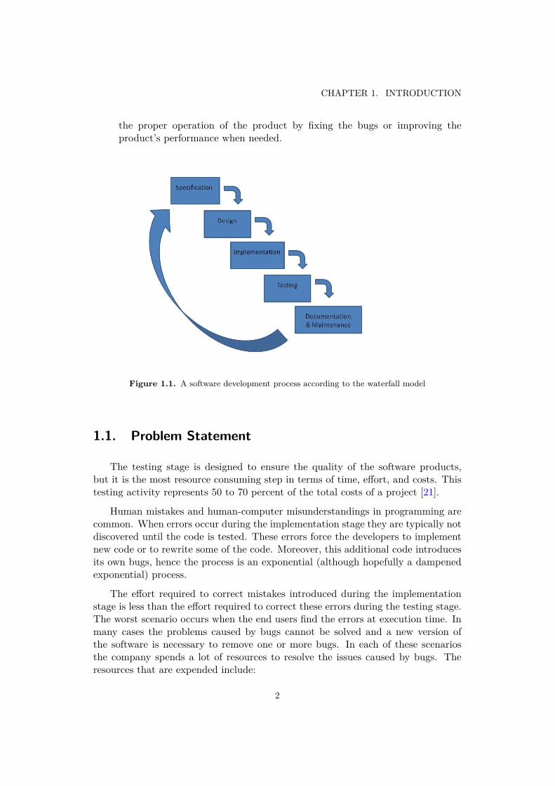
This software development process occurs whenever a company wants to createa new software product or improve an existing product. This development processconsists, of at least, the following steps: specification, design, implementation,validation, documentation, delivery, and maintenance [31]. The waterfall modelof this process is shown in Figure 1.1. Due to simplicity the waterfall model isexplained but the scope of this thesis project are also applicable to different softwaredevelopment models. These steps are:

Specification The customers determine the requirements and the purpose of thesoftware.

Design The managers of the project together with the programmers define themethodology and design of the product.

Development The programmers develop the new software.

Testing Here the programs are tested looking for any bug that could came upwith present or future failures in the system. This stage is usually the mostresource consuming.

Documentation and Maintenance In this step the programs are documentedand maintenance starts. In the maintenance process programmers supervise

1

CHAPTER 1. INTRODUCTION

the proper operation of the product by fixing the bugs or improving theproduct’s performance when needed.

Figure 1.1. A software development process according to the waterfall model

1.1. Problem Statement

The testing stage is designed to ensure the quality of the software products,but it is the most resource consuming step in terms of time, effort, and costs. Thistesting activity represents 50 to 70 percent of the total costs of a project [21].

Human mistakes and human-computer misunderstandings in programming arecommon. When errors occur during the implementation stage they are typically notdiscovered until the code is tested. These errors force the developers to implementnew code or to rewrite some of the code. Moreover, this additional code introducesits own bugs, hence the process is an exponential (although hopefully a dampenedexponential) process.

The effort required to correct mistakes introduced during the implementationstage is less than the effort required to correct these errors during the testing stage.The worst scenario occurs when the end users find the errors at execution time. Inmany cases the problems caused by bugs cannot be solved and a new version ofthe software is necessary to remove one or more bugs. In each of these scenariosthe company spends a lot of resources to resolve the issues caused by bugs. Theresources that are expended include:

2

1.2. GOALS

Capital Many different tests are needed to find the errors in the code. Developingand maintaining these tests also costs money.

Time Locating bugs usually takes a lot of time.

Effort Locating and correcting bugs is a hard task.

It is easy to see that the earlier a bug is detected and corrected, the lower thetotal cost. Consequently, many companies have decided to invest in new ways todetect and correct bugs as early in the overall process as possible [18], for exampleby adopting agile programming, deriving the program from formal specification,and other techniques.

1.2. Goals

The main goal of this thesis project is to improve the quality of software.Improving the quality of this software implies a reduction in development andmaintenance costs, hence a reduction in the costs of the whole company. Higherquality software might also increase customer satisfaction and confidence in thecompany and its products [18]. To carry out this improvement this thesis projectwill focus on predicting the presence of bugs in the early stages of the developmentprocess. This prediction is based on computing software metrics over the software’ssource code.

With regard to studies of rapid bug prediction, this project will contribute byshowing that there is a relationship between software metrics and the presence ofbugs and that the presence of bugs can be estimated by using a neuro-fuzzy hybridmodel.

1.3. Scope

The scope of this project is a tool to predict with high accuracy the existence ofbugs in code. This tool will facilitate the detection of the most error prone modulesin a programs while the software is being developed. Furthermore, this tool willallow users to:

correct bugs during the development stage that would otherwise not be founduntil the testing stage (this will be done by refactoring of the source code);

be aware of which modules have to be tested carefully during the testingprocess; and

learn (by suitable training) a programming style which is less error prone.This can be done by learning which programming styles have good feedback

3

CHAPTER 1. INTRODUCTION

from the tool.

1.4. Target Audience

This thesis may be interesting for those programmers who want to improve thequality of their code. It should be interesting for all enterprises, especially thosethat develop software products. The project also contributes to research on softwaremetrics and their relationship with bugs and to the investigations of several different(and useful) regression models.

1.5. Methodology

This thesis project started with an analysis of the problem statement (given inSection 1.1). Software metrics were previously identified to be predictors, thus thisthesis project considered a number of different metrics and their contribution tobug prediction. A selection of the best means to compute these metrics was alsodone. Subsequently several different regression models were examined in order tofind a model that successfully relates these metrics with bugs. Once the objectivewas clear, implementation of a prototype started.

A neuro-fuzzy hybrid model was chosen because, as the literature shows, thismodel has good capabilities together with regression models. Hybrid models are animprovement over neural network models which have no initial parameters defined.After the neuro-fuzzy hybrid model was chosed the following steps were taken:

1. Extraction of the software metrics of the source codes with the CCCC program[23].

2. Extraction of the number of known bugs for this source code from a repositoryof trouble reports.

3. Clustering of the metrics with the R program [26].

4. Implementation, training, and testing of a neural network in R.

5. Creation of a tool that would compute the software metrics and estimate thenumber of bugs in source code that is input to this tool.

4

1.6. STRUCTURE

1.6. Structure

Chapter 1 introduces the objectives and the motivation for this thesis project.

Chapter 2 gives the background necessary for reading this thesis and theknowledge needed to understand it. Chapter 2 starts with some definitions ofobject-oriented programming for those who are not familiar with this terminology.The chapter continues with an explanation of the most widely used softwaremetrics. The chapter concludes with a description of some of the most widely usedregression models, but focuses on neuro-fuzzy hybrid models, on neural networks,and clustering techniques.

Chapter 3 gives an overview of the model followed to create the tool.Chapter 3 begins with a brief explanation of the desired characteristics of the tooland continues with the selection of the programs, techniques, and models used inthis thesis project to relate software metrics and bugs.

Chapter 4 describes in detail the implementation of the neuro-fuzzy hybridmodel to finalize analyzing its results and verifying its quality.

Chapter 5 explains the functionalities of the final tool and the results of usingthis tool.

Chapter 6 presents some conclusions.

Chapter 7 proposes future work which can be done to improve the tool.

Furthermore, appendixes A and B contain further information about the tool.To conclude, appendixes C and D contain the introduction and conclusions of thismaster thesis in spanish, and E and F contain the budget and the specificationsalso in spanish.

5

Chapter 2

Background

This chapter presents the background of the thesis. It is divided into twosections. Section 2.1 gives the necessary knowledge to understand the selectedsoftware metrics and how they are estimated. Section 2.2 gives an overview ofthe different regression models that were considered, subsequently focusing on theneuro-fuzzy model. A number of different clustering techniques and artificial neuralnetwork models are explained.

2.1. Software Metrics

Software metrics are quantitative measures of the attributes of a program. Thereare three kinds of software metrics: procedure metrics, project metrics, and productmetrics [16].

Procedure metrics measure the resources (time and cost) that a programdevelopment effort will take. They are useful for the administration andmanagement of the project.

Project metrics give information about the actual situation of the project.These metrics include costs, effort, risks, and quality. These are used toimprove the development process of the project.

Product metrics assess quality information about the program. These metricsfocus on reliability, maintainability, complexity, and reusability of all or partof the software developed for the program.

The reliability of these software metrics as predictors bugs has been studiedand tested by many researchers [6, 9, 3], who have used different regression modelsapplied to different languages. All of these researchers have claimed software metricsto have good capabilities as indicators of bugs.

7

CHAPTER 2. BACKGROUND

2.1.1. Basic Concepts

We will use a number of basic concepts in this thesis. Below is a short descriptionof each of these concepts for the reader’s reference.

OOP (Object-Oriented Programming) OOP is a programming style based onthe use of objects. Thus, programs are made of objects that are manipulatedto perform a specific task.

Object An object is an instance of a class which has been defined with someproperties, specifically: attributes and methods.

Class A class is the template used to create objects. Different objects of the sameclass have a similar structure.

Method A method is subroutine of a class that performs an operation.

Attribute An attribute is a member variable of a class.

Inheritance Inheritance is the process where by an object acquires some propertiesand methods of another class.

Children A child or subclass is the class that inherits properties and methods inan inheritance process.

Ancestor An ancestor or superclass is the class from which another class inheritsproperties and methods in an inheritance process.

2.1.2. Definition of Metrics

Currently, the goal of software developers is to offer the best quality in theirprograms without increasing the amount of resources needed for the development ofthis software. For this reason in this study we will focus on product metrics. Thesemetrics are summarized in Table 2.1. In despite of the metric definitions given inthe Table 2.1, many researchers claimed that software metrics lacked mathematicalstrictness and other desirable properties [33, 35]. Therefore, they considered theestimates of these metrics to be unreliable. Consequently, in 1994, Chidamber andKemerer described in [6] six metrics which are now called ’CK metrics’. These sixmetrics have been successfully correlated with the likelihood of error in software inmany investigation (in [30] for Java language and in [3] for C++ language).

8

2.1. SOFTWARE METRICS

Table 2.1. Object Oriented Metrics

Name/Acronym

Description

Lines of Code(LOC)

Total number of lines of code. LOC may or may not take into consid-eration blank and comment lines. LOC is related with the size of thesource code subject to bugs. The reliability of this metric has alwaysbeen questioned because although the probability of mistakes increaseswith the opportunity to make them, it has been observed that when thecomplexity of the code is low, the number of bugs is also small even ifthere are many lines of code.

Number ofattributes(NOA)

The number of public, private, and inherited attributes.

Number ofmethods(NOM)

The number of public, private, and inherited methods.

McCabe’scyclomaticcomplexity

This metric can be defined in a given class as the sum of the complexityof the methods defined for the class. It estimates the complexity as thenumber of linearly independent paths that can be followed in the class.In 1976 Thomas J.McCabe introduced this new metric in [25]. Whenthe value of McCabe’s metric exceeds some threshold for one module(according to [11] a value higher than 10), then the module should besplit into smaller modules.

Fan in/ Fanout These two metrics concern the number of classes which reference theclass/the number of classes referenced by the class. Fan in and Fanoutdescribe the relationship between a given class and its environment.These metrics are related to the flow structure of the system. SallieHenry and Dennis Kafura introduced these new metrics in [15] in 1981.

Informationflow complexity

This metric is a measure of the complexity of the code in terms of itsfan in and its fan out. This metric is computed using equation 2.1.

IFc = (Fanin ∗ Fanout)2 (2.1)

The greater the complexity of the code the greater the probability ofthere being an error. Sallie Henry and Dennis Kafura introduced thisnew metric in [15] in 1981.

The CK metrics are described in Table 2.2 for a given class.

9


Table 2.2. Object Oriented CK Metrics

Name/Acronym

Description

WeightedMethods PerClass (WMC)

This metric is the sum of the complexity of the methods defined in theclass when the complexity value assigned to each method is 1. Thismetric is computed using equations 2.2 and 2.3.

WCM =n∑i=1

Ci (2.2)

when Ci = 1,WCM = n (2.3)

This metric gives an approximation of the time and effort needed todesign and maintain the class. This metric captures the observationthat the more complex the methods of a class, the more error prone thisclass is.

Depth ofInheritanceTree (DIT)

In an inheritance tree DIT is the maximum length from a node in thetree to the root. High values of DIT means that the classes are reusingthe methods of its ancestors, thus these classes were well defined whichenabled their reuse. However, a high value of DIT implies that thestructure of the code is more complex, and that it is more complicatedto test.

Number ofChildren(NOC)

NOC is the number of direct subclasses which belong to a class. WhenNOC is high, a change in the class can potentially affect many differentclasses.

Couplingbetween objectclasses (CBO)

One class is coupled with another when it uses the methods or instancevariables of the latter. CBO is the number of other classes which arecoupled with a specific class. When CBO is high, then one error in theclass could affect many classes in the program. CBO is a measure of theindependency of the class.

10

2.1. SOFTWARE METRICS

Name/Acronym

Description

Response For aClass (RFC)

RFC is the number of methods invoked when an object of the classreceives a message. The value is computed according to equation 2.4.

RFC = |RS|, where RS = {M} ∪alli {Ri} (2.4)

Where M is the set of all methods in the class and Ri is the set ofmethods invoked by method i. Classes with a low value of RFC aresimpler, hence it is easier to debug them. Classes with a high value ofRFC have a large and potentially highly distributed effect, hence theyare harder to debug as the number of messages triggered by one messagecan expand rapidly.

Lack ofCohesion inMethods(LCOM)

LCOM is the number of methods pairs belonging to the class that donot share instance variables minus the number of those which do. Thismetric is calculated using equation 2.5.

LCOM ={|P | − |Q| if |P | > |Q|0 otherwise (2.5)

Where P is the number of methods in the class that do not use the sameinstance variables (analyzed by pairs) and Q is the number of methodsthat share them. The larger the value of LCOM is, the lower the cohesionof the class. A high value of LCOM indicates that the class shouldbe divided into subclasses, as its methods realize different objectives(as they represent computations over variables that are increasinglyindependent with increase LCOM value).

These metrics are only a sample of all the metrics which can be used (and havebeen used) to analyze the characteristics of source code. These metrics have beingused in many studies that have attempted to predict bugs in software. Today thesemetrics are used by many enterprises to estimate the quality of their programs.

An additional metric called BUGFIXES is based on the results of the datasheetused by Marco D’Ambros and Romain Robbes in 2010. In [9] they described howthey created a datasheet for five different systems written in java: Eclipse JDT Core,Eclipse PDE UI, Equinox framework, Mylyn, and Apache Lucene. Their goal wasto predict the efficiency of different types of metrics applied to different programs.For this prediction, they introduced a new metric called BUGFIXES (see Table 2.3.

11


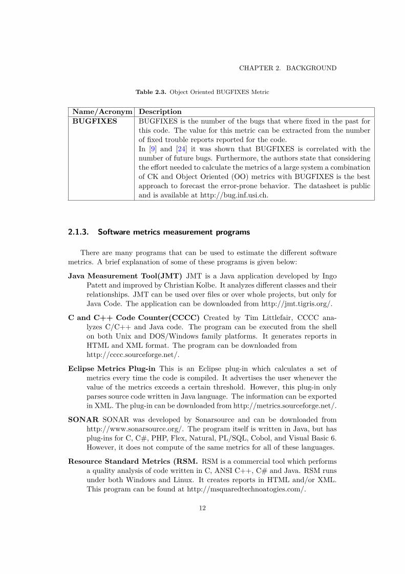
Table 2.3. Object Oriented BUGFIXES Metric

Name/Acronym DescriptionBUGFIXES BUGFIXES is the number of the bugs that where fixed in the past for

this code. The value for this metric can be extracted from the numberof fixed trouble reports reported for the code.In [9] and [24] it was shown that BUGFIXES is correlated with thenumber of future bugs. Furthermore, the authors state that consideringthe effort needed to calculate the metrics of a large system a combinationof CK and Object Oriented (OO) metrics with BUGFIXES is the bestapproach to forecast the error-prone behavior. The datasheet is publicand is available at http://bug.inf.usi.ch.

2.1.3. Software metrics measurement programs

There are many programs that can be used to estimate the different softwaremetrics. A brief explanation of some of these programs is given below:

Java Measurement Tool(JMT) JMT is a Java application developed by IngoPatett and improved by Christian Kolbe. It analyzes different classes and theirrelationships. JMT can be used over files or over whole projects, but only forJava Code. The application can be downloaded from http://jmt.tigris.org/.

C and C++ Code Counter(CCCC) Created by Tim Littlefair, CCCC ana-lyzes C/C++ and Java code. The program can be executed from the shellon both Unix and DOS/Windows family platforms. It generates reports inHTML and XML format. The program can be downloaded fromhttp://cccc.sourceforge.net/.

Eclipse Metrics Plug-in This is an Eclipse plug-in which calculates a set ofmetrics every time the code is compiled. It advertises the user whenever thevalue of the metrics exceeds a certain threshold. However, this plug-in onlyparses source code written in Java language. The information can be exportedin XML. The plug-in can be downloaded from http://metrics.sourceforge.net/.

SONAR SONAR was developed by Sonarsource and can be downloaded fromhttp://www.sonarsource.org/. The program itself is written in Java, but hasplug-ins for C, C#, PHP, Flex, Natural, PL/SQL, Cobol, and Visual Basic 6.However, it does not compute of the same metrics for all of these languages.

Resource Standard Metrics (RSM. RSM is a commercial tool which performsa quality analysis of code written in C, ANSI C++, C# and Java. RSM runsunder both Windows and Linux. It creates reports in HTML and/or XML.This program can be found at http://msquaredtechnoatogies.com/.

12

2.2. REGRESSION MODELS

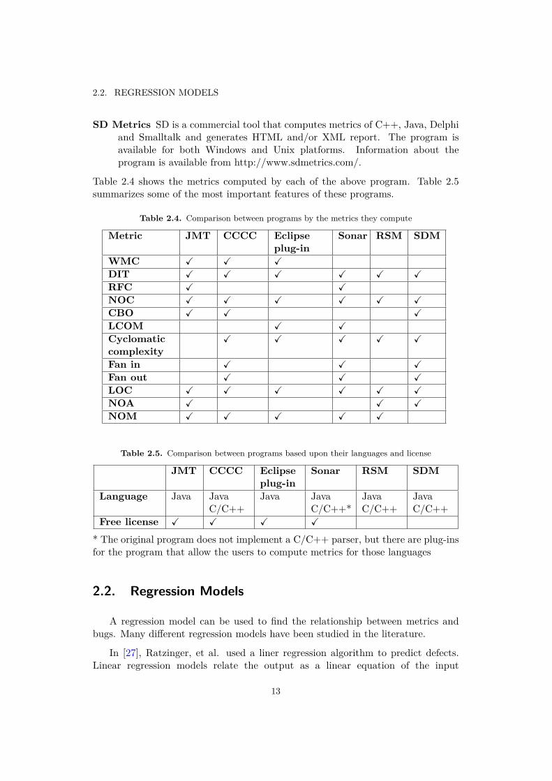
SD Metrics SD is a commercial tool that computes metrics of C++, Java, Delphiand Smalltalk and generates HTML and/or XML report. The program isavailable for both Windows and Unix platforms. Information about theprogram is available from http://www.sdmetrics.com/.

Table 2.4 shows the metrics computed by each of the above program. Table 2.5summarizes some of the most important features of these programs.

Table 2.4. Comparison between programs by the metrics they compute

Metric JMT CCCC Eclipseplug-in

Sonar RSM SDM

WMC X X XDIT X X X X X XRFC X XNOC X X X X X XCBO X X XLCOM X XCyclomaticcomplexity

X X X X X

Fan in X X XFan out X X XLOC X X X X X XNOA X X XNOM X X X X X

Table 2.5. Comparison between programs based upon their languages and license

JMT CCCC Eclipseplug-in

Sonar RSM SDM

Language Java JavaC/C++

Java JavaC/C++*

JavaC/C++

JavaC/C++

Free license X X X X

* The original program does not implement a C/C++ parser, but there are plug-insfor the program that allow the users to compute metrics for those languages

2.2. Regression Models

A regression model can be used to find the relationship between metrics andbugs. Many different regression models have been studied in the literature.

In [27], Ratzinger, et al. used a liner regression algorithm to predict defects.Linear regression models relate the output as a linear equation of the input

13


attributes. In their study they create a predictor for defect densities by using datamining techniques. This predictor had good results (with a correlation coefficientbetween predictions and real values greater than 0.7 over 1) in the three softwareprojects that they tested: ArgoUML and the Spring framework (both open sourceprojects with 5,000 and 10,000 classes respectively), and one commercial systemwith more than 8,600 classes. All of these three programs were written in Java.

Today research about metrics and bugs no longer utilizes linear models, as recentstudies has shown that linear models do not provide good performance due to thecomplexity of the relation between metrics and bugs [18, 8]. Today machine learningbased models are widely used. These models are based on the learning capacityof algorithms which are trained with patterns. The most widely used learningalgorithms to implement bug prediction models are decision trees, classifiers, andneural networks.

In 2012, Singh and Verma [30] utilized two different models of machine learning:J48 (a decision tree) and naïve Bayes algorithm (classifiers). With these modelsthey got an accuracy of 98.15% and 95.58% (respectively) using the CK metricsas predictors. Furthermore, Ahsan and Wotawa [1] used regression models anddecision trees to predict bugs in C language programs. In their work decision treesseemed to give better predictions (with an accuracy of 97%).

However, in [29] Gray and MacDonell claim that neuro-fuzzy hybrids are thebest regression model in comparison with neural networks and fuzzy logic models.Gan and Harris use topology clustering techniques to define the neural networksand to give the initial parameters [13]. A similar model was used by Jin, et al. [18]where a Fuzzy c-means (FCM) clustering with a Fisher’s Linear Discriminant (FLD)method is used to define the initial parameters for a Radial Basis Function (RBF)neural network. This model was used to determine the probability of errors of 70C++ classes. The model was trained with 106 classes and it showed an accuracyof 90% in comparison with 87.14% for logistic regression.

In 2012, a new model was developed by Couto, et al. [8] where the GrangerCausality test was used to establish the relationship. This test was suggested byClive Granger to predict how the past events occurring in one series (a numericalsequence) influenced events in other series. The model uses the next bivariate auto-regressive model. Couto, et al. predicted with the Granger’s Causality test theorigin of 64% to 93% of the bugs detected in the systems studied by D’Ambros etal. in their datasheet [9]. The datasheet contains 1041 classes from Eclipse JDTCore, 1924 from Eclipse PDE UI, 444 from Equinox, and and 889 from Lucene witha total of 5028 (known) bugs in the four systems.

14


2.2.1. Artificial Neural Networks

Artificial Neural Networks (ANN), also called Neural Network (NN), is amathematical model which aims to learn by training the behavior of a specificsystem. This model was inspired by the behavior of the brain when learning andthis model has been used to establish relationships between a set of inputs andoutputs [7, 14].

There are two main neural network architectures. The difference is the connec-tion between the layers. These two architectures are:

Feed-forward networks. In this architecture the signals advance from the inputto the output only in one direction: forward. This architecture is widely usedfor pattern recognition.

Feedback networks. These networks have feedback loops so the signals moveboth forward and backward until they reach an equilibrium. This equilibriumchanges every time an input is modified.

A simple example of a neural network is shown in Figure 2.1. It consists of threelayers: the input layer fed wth the input data, the hidden layer composed of multipleprocessing elements working in parallel, and the output layer. All the elements(analogous to neurons) are connected by links of different weights. Figure 2.2 showsone neuron in such a network.

Figure 2.1. An example of an artificial neural network

When a neuron is activated its output contributes to the global output of thesystem. The activation state is decided by analyzing the result of the activationfunction over the inputs and their weights. The global output depends on the weightof the different links and these weights are adjusted such that the system gives the

15


correct outputs. The process responsible for this adjustment in weights is called thelearning or training process.

Figure 2.2. A neuron of a generic artificial neural network

There are three types of learning processes:

Supervised learning In supervised learning the system knows the input data andtheir expected output. Training consists of minimize the error between thecurrent result and the desired output. The error is defined by equation 2.6.

E = 12

k∑1||yi − y′i||2 (2.6)

Unsupervised learning In unsupervised learning the system only has input data.These type of algorithms are commonly used for pattern classification.

Reinforcement learning In reinforcment learning the system knows the inputdata and which outputs are correct or incorrect.

16


2.2.1.1. Backpropagation Neural Network

Backpropagation Neural Networks uses the backpropagation (BP) algorithm,which is a supervised learning algorithm used in feed-forward architectures. Back-propagation is the most widely used algorithm in ANNs. The signals travel forwardin the topology and sends backward the estimated error. A hidden neuron of thisnetwork is shown in Figure 2.3

Figure 2.3. A neuron of a backpropagation neural network

If is ~x the input data and Wi,j are the weights between the input neuronsi and the hidden neurons j, then the activation function of this algorithm is givenby equation 2.7.

hi,j(xi,Wi,j) =n∑1xi ∗Wi,j > threshold (2.7)

The most used output function for the neuron is the sigmoidal function given inequation 2.8

11 + ehi,j(xi,Wi,j) (2.8)

17


where h is the activation function. The BP algorithm minimizes the error functionby using the method of gradient descent, i.e., in this algorithm the sum of thegradient of the error function for every hidden neuron is calculated in every iteration.Once the total error is computed, then the algorithm tries to modify the weights ofthe links between the hidden layer and the output layer to minimize this sum (asdescribed by equaiton 2.9).

∇E = ( ∂E∂w1

,∂E

∂w2,∂E

∂w3, . . . ,

∂E

∂wn) = 0 (2.9)

The weights are incremented by

∆wi = γ ∗ ∂E∂wi

, i = 1, ....., n (2.10)

More information about the backpropagation algorithm can be found in [28].

2.2.1.2. Radial Basis Function Neural Network

A Radial Basis Function (RBF) Neural Network is also a feed-forward network.In this topology, the neurons are defined to be activated when the input samplebelongs to their cluster. Membership is decided by estimating the Euclideandistance between the input data and the weight of the links with the following layer.Unlike the BP algorithm, the RBF algorithm fixes the input weights of the hiddenneurons and tries to optimize the weights of the following layers. In this topologyhidden neurons use a non-linear activation function. There are many possibilitiesfor this function, but the most usual it is the Gaussian function given in equation2.11.

H(x) = e−β~x2 for some β > 0 (2.11)This can be approximated as:

h(x) = e−||~x− ~ci||2

σ2 (2.12)

This choice of function implies that when the distance to the center of the clusteris small, then and only then does the neuron have a perceptible value. This valuedecreases rapidly to zero as the distance from the center of the clusters increases.

The output function of the network is therefore of the form shown in equation2.13.

F (x) =k∑i=1

~ci ∗ h(~x) (2.13)

This algorithm can implement both supervised and unsupervised learning. Itcan be used for classification, times series prediction, approximation function, etc.

18


The main problem of neural networks is that the topology (specifically thenumber of neurons) should be defined a priori. For that reason, clusteringtechniques are frequently used to extract information which is hidden in the data,thus enabling us to make the best choice of the number of neurons. Clusteringtechniques also can give initial values for the links between the two first layers.

In addition, both BP and RBF neural networks have the same major drawbackin that both are strongly dependent upon their initial parameters. This meansthat the network can come trapped in a local minimum instead of finding a globalminimum if the network starts close to a local minima. In [22] both BP and RBFneural networks were studied and compared by Leonard and Kramer. Leonard andKramer claim that a RBF NN performs better in terms of identifying samples (agiven combination of inputs) located far from the training data. It was also claimedthat in general, RBF NN are faster than BP NN by one decimal order of magnitude.

2.2.2. Clustering

Clustering is the task of divide a set of objects into clusters. Every cluster isformed by a group of objects which share similarities such that objects belonging todifferent cluster are as different as possible. Clustering is therefore an unsupervisedclassification mechanism which aims to reduce the dimension of the input set ofdata by discarding redundant information. Clustering techniques are widely usedin pattern recognition and classification, and image processing.

The objects ~x ∈ Rn are usually observations of a phenomenon collected from nmeasurements, ~x = (x1, x2, . . . , xn). An example of a cluster in two dimensions isshown in Figure 2.4. In this example the data has been divided into three clusters.

There are two different techniques regarding applying this kind of partitioningto a data set: hard partitioning and soft partitioning.

Hard Clustering implements hard partitioning. In this technique the objectsof the data set belong to one and only one cluster. Figure 2.4 shows this type ofpartitioning.

19


Figure 2.4. Hard partitioning over a data set

Soft Clustering utilizes soft partitioning (also called fuzzy partitioning) allow-ing objects to belong to multiple clusters. Each object can be a member of a clusterto a certain degree, ranging from 0 to 1. An example of this is shown in Figure 2.5.

Figure 2.5. Soft partitioning over a data set

20


Regarding the method used to split up the cluster, multiple algorithms can beused. In this thesis the technique we will use is linear optimization algorithms.These algorithms are used to search for the local minima of an objective function.

2.2.2.1. Fuzzy c-means

A fuzzy clustering algorithm that is widely used in software metric analysisis fuzzy c-means (FCM). This agorithm divides the objects into equal sphericalclusters by using as the distance norm the Euclidean distance. This technique aimsto optimize the function shown in equation 2.14. This function was first proposedby Bezdek in [17].

Jm(Z;U, V ) =c∑i=1

N∑k=1

(µmik)||zk − vi||2 (2.14)

The algorithm is based upon the following steps [2]:

1. Initialize the membership matrix.

2. Compute the clusters model.

3. Compute the distance between the sample and the clusters

4. Update the membership matrix

The output of the algorithm it is the membership matrix and the centers of theclusters.

Due to the use of the Euclidean distance to define the clusters, this algorithmonly gives good results when the data set forms spheroids of the same size or whenthe distance between the different clusters is large. As a result the applicability offuzzy algorithms is dependent upon the shape of the clusters. In the case of FCMeach cluster will have a spherical shape, but the cluster might also be ellipticalor rectangular. The decision upon the shape is very important as it represents alimitation of the algorithm which forces the algorithm to find clusters with thatspecific shape even when is not present in the data.

One approach to solve this problem is the use of the Gustafson-Kessel algorithm.

2.2.2.2. Gustafson-Kessel Algorithm

In contrast to FCM the Gustafson-Kessel (GK) algorithm implements anadaptive distance norm so it can distinguish the different geometrical forms whichthe patterns perform [20, 2].

21


The operating of the algorithm is similar to FCM, but the distance used isdefined in equation 2.15.

D2ikAi

= (zk − vi)TAi(zk − vi) (2.15)

It should be noted that the GK distance is the same as the FCM distance when A isthe identity matrix. In this case, A is described by the Lagrange multiplier methodfor every i cluster as:

Ai = [ρidet(Fi)]1nF−1

i (2.16)

Where Fi is the fuzzy covariance matrix:

Fi =

N∑k=1

(µik)m(zk − vi)(zk − vi)T

N∑k=1

(µik)m(2.17)

Thus the objective function is:

J(Z;U, V,Ai) =c∑i=1

N∑k=1

(µmik)D2ikAi

(2.18)

One example of the results that can be obtained from this algorithm is shownin Figure 2.6. Note that this is the same data set as used in Figures 2.4 and 2.5

Figure 2.6. Results of Gustafson-Kessel Algorithm over a data set

22


The main problem of these algorithms is that the number of clusters, thefuzziness exponent, and the tolerance must be determined a priori [19].

Another problem due to the choice of algorithm is that they are stronglydependent on the initial parameters, thus they may converge to different localminima for different initializations. This also means that the resulting NN maynot correctly predict the output for an input that is not nearly equivalent to asample from the training set.

The number of clusters K is the most critical parameter. This parameter is hardto determine because it has to be defined in advanced, usually without knowledgeof the actual number of cluster that are present in the data set. Once this numberis defined, the algorithm will look for that number of cluster whether they exist ornot.

The fuzzifier exponent, m, is related to the level of fuzziness of the algorithm.When m→∞, it is completely fuzzy and it becomes less fuzzy as m decreases. Themost frequent value for this parameter is 2.

Finally the fuzzy algorithm may or may not converge to a clear minimum. Forthis reason a tolerance parameter is needed. This paramter defines the accepteddifference between two successive iterations that reflects the fact that the algorithmhas found an acceptable minimum

23

Chapter 3

Analysis

In this chapter an overview of the model followed to create the final tool. InSection 3.1 the specifications and limitations of the tool are given. In Section 3.2the background material is analyzed and the software metrics and regression modelare chosen.

3.0.3. Specification

The specifications of the tool are:

The final tool should implement two functions: predict the actual number ofbugs of a given set of source code; and allow the user to train the network toadapt it to different environments, i.e. different programming languages.

Even though the program should work for different programming languagesthe predictor in this thesis project will analyze only source code written inC++.

The tool should be run from the Linux shell in order to be easily incorporatedinto the existing project running within the department.

The tool should be implemented by using license free or open source programs.

3.0.4. Selection of the model

The main goal which need to be reached in order to create the tool is the creationof a model which relates software metrics with the number of bugs in a set of C++source code.

The background literature described in Chapter 2 has shown that softwaremetrics and bugs have been related by many different models. There are also

25

CHAPTER 3. ANALYSIS

different metrics that can be used. Thus, it is necessary to select the metrics andthe model that are most useful for our goal.

Regarding the program, we have to take into consideration two main restrictions:the first restriction is that this program should analyze C/C++ language becausethis is the programming language used by the department; and the second restrictionis that the program needs to include only be license free or open source as part ofthe tool. There are only two programs in Table 2.5 that fulfill these requirements:CCCC and Sonar. Sonar has a free plug-in that parses source code written inC/C++ but is very limited (it does not implement the same features as the originalprogram) so we discarded this program. Consequently, the program selected tocompute the metrics is CCCC-C and C++ Code Counter.

Regarding the metrics, CCCC calculates all of the metrics but three: RFC,LCOM, and NOA. RFC and LCOM were also excluded in the study carried out bySubramanyam and Krishnan in [32] due to the complexity of their computation. Intheir study they claim that the effect of exclude RFC was limited and that LCOMrather than providing useful information may cause alterations in the results owingto the lack of a solid definition. Lastly, NOA has not been considered in manystudies. In this thesis project we will also not consider NOA. In addition, we alsoeliminate NOM from our list of metrics, because NOM has the same value as WCMwhen the complexity value assigned to each method is 1.

Concerning the regression model, in [22] Leonard and Kramer performed acomparison between BPNN and RBFNN. They claim that BPNN classifies thesamples arbitrarily when the samples are far from the training data. In contrastRBFNN classifies samples according to the distance between the samples and thetraining data. Thus, Leonard and Kramer claim that a RBFNN results in betterperformance in terms of identifying new samples. Therefore, in this thesis projectRBFNN is used to relate the software metrics of a code with its bugs. Furthermore,we agreed with Gray and MacDonell [29] that a neuro-fuzzy hybrid is the bestoption to implement regression models. Hybrid models implement neural networkswith the improvement that the initial parameters are defined by the prior clustering.This model is also supported by [34], where Wang and Shang showed that fuzzyclustering RBFNNs have better capabilities in pattern classification than normalRBF networks.

Finally we decided to use FCM. The main reason was that RBFNN (as FCM)utilizes the Euclidean distance to determine which samples should activate thedifferent hidden neurons. Consequently it will not be useful to look for any othertype of shape in the input data.

26

Chapter 4

Model implementation

In this chapter the implementation of the model is explained in detail. Section4.1 defines how clustering techniques are related with the neural networks tocreate neuro-fuzzy hybrid models. Section 4.1 finalizes with the definition of someparameters that can be used to ensure the quality of the model. In Section 4.2 thesoftware metrics’ extraction is explained. In Section 4.3 and 4.4 respectively theFCM and RBFNN implementation are specified. Finally in Section 4.5 the resultsof the model are analyzed.

4.1. Hybrid topology

The creation of the final tool started with the implementation of the neuro-fuzzyhybrid model. This hybrid topology is composed of a primary stage of clusteringfollowed by a neural network. The methodology is the following: first we divided thedata samples into training samples and testing samples. Each data sample containsthe software metrics of one module. We use the training samples to train the modeland the testing samples to analyze its performance. Once we have the training setwe normalized it between 0 and 1, in order to limit the upper bound of the inputdata to the network. Subsequently we applied the clustering technique, in this casefuzzy c-means, over the training set and we obtained the center of the c clustersdefined to the algorithm. Later we created the radial basis neural network wherewe use the centroids of the clusters to determine the number of hidden neurons andthe initial weight of the links between the input layer and the hidden layer. Finally,as is shown in Figure 4.1, we used the training samples to train the network.

27

CHAPTER 4. MODEL IMPLEMENTATION

Figure 4.1. Example of an hybrid topology with 5 clusters

After training the model we used the testing data samples to verify its capabilityas a bug predictor. The quality of the model was evaluated in terms of the followingindicators:

Confusion matrix The confusion matrix of a neural network shows its classifica-tion results over a data sample. This matrix is shown in Table 4.1. In thismatrix a module is valuated as 0 when it is non buggy and as 1 when it is.

Table 4.1. Confusion Matrix

Predicted module=0 Predicted module=1Actualmodule=0

f 00 f 01

Actualmodule=1

f 10 f 11

From this matrix we can derive the following measures:

Accuracy Accuracy is the ratio of the correctly predicted modules to thetotal predicted modules.

Accuracy = f00 + f11f00 + f01 + f10 + f11

(4.1)

Precision Precision is the ratio of the correctly predicted buggy modules tothe total modules that are predicted to be buggy. The lower the precision,

28

4.2. EXTRACTION OF METRICS AND BUGS

the more effort is wasted in testing free error modules.

Precision = f11f01 + f11

(4.2)

Recall Recall is the ratio of the correctly predicted buggy modules to thetotal modules that are actually buggy. The lower the recall, the morebuggy modules go undetected.

Recall = f11f10 + f11

(4.3)

F-measure The F-measure is a combination between precision and recall. Itconsiders the tradeoff between both measures.

F −measure = 2 ∗ Precision ∗ recallPrecision+Recall

(4.4)

Receiving Operating Characteristic (ROC) The ROC curve of the network isalso plotted. The ROC shows the tradeoff between correctly predicted buggymodules and wrongly predicted buggy modules. In [36] it is claim that thegreater the area under the curve, the greater the quality of the neural network.

Root Mean Square (RMS) RMS shows the difference between the expectedoutput value and the actual output value. The lower the RMS, the greaterthe quality of the network. RMS is calculated in [39] as shown in Equation4.5.

RMS =

√√√√√ n∑i=1

(yactualoutput − yexpectedoutput)2

n(4.5)

4.2. Extraction of metrics and bugs

In this thesis project the extraction of the software metrics was done by twodifferent methods. We used the CCCC program to extract the metrics which canbe obtained from the source code and we created a simple script to extract from arepository of trouble reports the BUGFIXES metric. The actual number of bugsin this code was also extracted from the same repository. Note that here we areassuming that all of the bugs have been detected in this repository. We believethat this is a relatively safe assumption because the lifetime of the program is largeenough to have reported all the bugs.

29


4.2.1. Extracting the metrics

In order to extract the metrics we used the CCCC- C and C++ Code Counterprogram. This program can be downloaded from http://cccc.sourceforge.net/.

CCCC extracts the metrics WMC, DIT, NOC, CBO, McCabe’s Cyclomaticcomplexity, Fan in, Fan out, LOC, and information flow complexity from a givenfile or set of files of a directory.

In order to calculate these metrics the CCCC program divides the files intomodules. Every class as well as every namespace is considered as a module (in theC++ environment). Functions which do not belong to any of these structures aremerged as part of the module "Anonymous".

In our program we wanted to perform a class-level bug prediction because ObjectOriented programs are built over classes so we did not use the information givenby the "Anonymous" file to create our predictor. We did not use either the metricsgiven by modules for which any definition or member function had been identifiedor modules which triggered a parse failure in CCCC, i.e. protected classes.

It is important to notice that CCCC has some limitations in computing metrics,therefore, a more specific definition of these metrics (as they are actually computed)will be given in Table 4.2.

Although the measures of the CCCC program are not perfect, they are claimedto agree with the manually calculated values of these metrics, under the samedefinitions, within 2-3% (i.e., the automatic extraction of these metrics has an errorof only 2-3%).

30

4.2. EXTRACTION OF METRICS AND BUGS

Table 4.2. CCCC metrics’ definition

Name/Acronym

Description

Lines of Code(LOC)

The total number of lines is calculated taking into account the numberof non-blank and non-comment lines. The preprocessor lines are treatedas blank lines and declarations of global data are ignored. However thenumber of lines may be overestimated as the program may count twicethe number of lines in the class definitions. This could occur becausethe algorithm counts the lines of a module as the sum of the lines of themodule itself plus the lines of its member functions. Thus, declarationsand definitions of the member functions in the body of the class will becounted twice.

McCabe’scyclomaticcomplexity

McCabe’s Cyclomatic Complexity value is approximated by countingthe commands which create extra paths in the execution of a class. Inthe case of C++ this means that it counts the number of the followingtokens: ’if’, ’while’, ’for’, ’switch’, ’break’, ’&&’ and ’||’.

Fan in/ Fanout These two metrics concern the number of classes which reference theclass/the number of classes referenced by the class. CCCC can onlyidentify the following relationships in a class: inheritance, instance ofa supplier class, and the existence of member functions which accep-t/return instances from/to a supplier class. However, it is often one ofthese relationships references a class, so both counts seems to be highlycorrelated.

Informationflow complexity

IF_c is calculated as the square of the product of the fan in and fan outof the current module.

WeightedMethods PerClass (WMC)

WMC is computed as the multiplication of the number of functionsof the current module times a weighting factor. The algorithm uses anominal value of 1 as weighting factor.

Depth ofInheritanceTree (DIT)

DIT is given by the length of the longest path of the inheritance treewhich ends at the current module.

Number ofChildren(NOC)

NOC is given by the number of modules that directly inherit the currentmodule.

Couplingbetween objectclasses (CBO)

CBO is the number of modules coupled with the current module eitheras clients or suppliers.

31


4.2.2. Extracting information about bugs

In order to implement supervised learning in the neural network the numberof actual bugs (the expected output of the system) has to be extracted from therepository. This thesis project trained of the network using a released version ofa product developed in Ericsson. For this program we extracted the number ofpreviously fixed bugs as well as the number of actual bugs from the repositorybased upon trouble reports recorded for the project.

We consider that every trouble reported indicates one bug in all the files whichhad to be changed to fix this bug.

Since CCCC parses the programs by modules and we extract the number ofbugs by files there is a discrepancy that had to be resolved. Our solution was toassign to every module the sum of bugs reported for the files which compose themodule.

4.3. FCM Clustering

We have implemented FCM in R using the package ’e1071’ which canbe downloaded from http://cran.r-project.org/web/packages/e1071/index.html. We applied the function ’cmeans’ with the method ’cmeans’ to the trainingset. There are three parameters that have to be defined a priori: the number ofclusters, the fuzziness exponent, and the tolerance.

Number of clusters

The number of clusters is defined as the number of groups into which the dataset is split during the clustering process. The number of clusters is the most criticalparameter because the algorithm will look for this number of clusters whether theyare present or not in the data set. Determining this parameter without previousstudy of the samples is, in general, a hard task. Therefore we will use someparameters which have been used in the literature to determine the optimum numberof clusters in a data set. These parameters are:

Xie.beni Proposed by Xuanli Lisa Xie and Gerardo Beni in [37], Xie.beni (XB)gives the ratio of the total variation of the partition and the centroids, andthe separation of the centroids vectors. Thus, it is function of the data set andthe center of the clusters. The minimum value of xie.beni under comparisonusually indicates the best partition.

XB =

c∑i=1

N∑k=1

(µ2ik)||zk − vi||2

N ∗mini 6=k||vi − vk||2(4.6)

32

http://cran.r-project.org/web/packages/e1071/index.html

http://cran.r-project.org/web/packages/e1071/index.html

4.3. FCM CLUSTERING

Fukuyama.sugeno Fukuyama.sugeno (FS) index, as shown in Equation 4.7, com-putes the difference between two terms combined with the fuzziness in themembership matrix: the compactness of the representation of the data set,and the degree of separation between each cluster and the mean of the clustercentroids. Low values of fukuyama.sugeno indicate good partitions [38].

FS =c∑i=1

N∑k=1

(µmik)(||zk − vi||2 − ||vi − v̄i||2) (4.7)

Partition coefficient and Partition entropy Proposed by Bezdek, the parti-tion coefficient (PC) and partition entropy(PE) indexes measure the fuzzinessof the partition. This means that both parameters measure how much theoverlapping is between the clusters in the data set.

The partition coefficient is given by Equation 4.8 (and takes on values in therange [1/c,1]).

PC = 1N

c∑i=1

N∑k=1

µ2ik (4.8)

The partition entropy is given by Equation 4.9 (and takes on values in therange [0, log(c)]).

PC = − 1N

c∑i=1

N∑k=1

µik loga µik (4.9)

We look for a value for the number of clusters which maximizes PC andminimizes PE [38].

Partition separation Index ( CS (Compact-Separate)Index) The partitionseparation index is created from the partition coefficient and the partitionentropy. It identifies compact, separate clusters. Large values of thiscoefficient means that the clusters are more compact and that they are wellseparated from each other [12]. However, for large data sets this index iscomputationally infeasible since a distance matrix between all the data termshas to be computed.

PS(c) =c∑i=1

N∑k=1

(µ2ik)

µM− e

(−minj 6=i

||vi − vj ||2

βT)

(4.10)

where

µM = max1≤i≤c

N∑k=1

µ2ik (4.11)

and

βT =

c∑i=1||vi − v̄||3

c(4.12)

33


Tolerance

Tolerance is determined by the program. The only value that is possible tochange is the number of maximum iterations. This maximum number of iterationsindicates to the program when to stop if the tolerance is not achieved. In this case,after running FCM several times, we observed that the algorithm always convergedto a solution.

Fuzziness exponent

We set the fuzziness exponent to the value of 2, as this is its default value.

4.4. RBFNN

The RBFNN used in this thesis project was implemented in R by using thepackage RSNNS [5]. This package uses the libraries of the Stuttgart Neural NetworkSimulator (SNNS) [39] which allows the package to implement many different neuralnetworks. A further description of the package is given in [4]. In order to implementour model we have used the low level interface of the package. The guide used toset up the RBFNN can be followed in [39].

The procedure was the following, first of all we created a SNNS object and wedefined the neurons of the network. We defined one input neuron for each metric,one hidden neuron for each cluster, and one unique output since we only wantedone output.

The desired output function of the network is shown in Equation 2.13. Tocompute this output, we defined the activation and the output function of theneurons as shown in Table 4.3. Each of these functions is described below the table.

Table 4.3. Output functions of the neurons of the network

Activation function Output functionInput neurons Act_Identity Out_IdentityHidden neurons Act_RBF_Gaussian:

h(q, p) = exp(e−βq )

where q = |x̄− t̄|2 and βis the bias of the neuron

Out_Identity

Output neurons Act_IdentityPlusBias Out_Identity

Act_Identity leaves the neuron active all the time.

Act_RBF_Gaussian activates the neuron with the distance between x̄ (thesample) and t̄ (the center of the cluster defined to the neuron). Values of x̄

34

4.5. EXPERIMENTS AND RESULTS

equal to t̄ yield an output of 1.0, while larger distances yield an output of 0.0.

Act_IdentityPlusBias activates the neuron with the weighted sum of allincoming activations and adds the bias of the neuron.

Subsequently, we initialized the weights of the links between the input layerand the output layer. First we initialized the network with the "RBF_Weights"procedure to copy unchanged the centroids of the clusters and the bias intothe different hidden neurons. Afterward we initialize the network with the"RBF_Weights_Redo" procedure which initializes the link weights between thehidden and the output layer. The data used in this initialization process are thetraining data set and their actual outcome values.

Finally, we train the network with the learning function "RadialBasisLearning".This function can modify different parameters within the network: the center vectorsof the hidden neurons, the bias of the hidden neurons, and the weights of all the linksas well as the bias of the output network. Furthermore, this function prevents theovertraining of the network by limiting the tolerated error in the output neuron.This overtraining occurs when the network learns the output of specific trainingsamples, but fails to learn the general behavior [22] -hence this overtraining shouldbe avoided.

Besides the regression model used to predict the probable number of bugs inthe modules, we have implemented a classification model. This classification modelidentifies whether there are or not bugs in a module. This implementation differsfrom the implementation of the regression model in the expected output value ofthe samples. Thus, in the classification model we assign an output value of 1 to allthe buggy modules of the training data set and an output value of -1 to the bugfree modules of the same set.

4.5. Experiments and results

In this thesis project we have parsed 1755 modules. From these modules, werandomly selected 1492 modules to train the model and 263 to test it (15%). Themajor drawback of this neuro-fuzzy hybrid model is that it is very dependent uponthe samples used to train it, therefore we selected different random combinations oftraining and testing data sets.

We performed the clustering over the training samples giving different valuesof the number of clusters ranging from 3 to 10. These results are shown in Table4.4 where the optimum values according to the definitions given in Section 4.3 arehighlighted.

35


Table 4.4. Cluster validity indexes

N.clusters XB FS PC PE CS10 0.001236 -51.1354 0.60137 0.92128 0.009669 0.0013346 -48.7097 0.60091 0.89828 0.001198 0.0003734 -50.3111 0.63003 0.81634 0.009747 0.0004622 -51.1411 0.63922 0.77780 0.004616 0.0006059 -50.1556 0.65346 0.71733 0.005005 0.0001928 -49.5123 0.69760 0.63600 0.007954 0.0000747 -51.7349 0.76467 0.48368 0.007953 0.0002578 -38.9224 0.75922 0.44721 0.00877

Thus, based upon the indexes given by xie.beni, fukuyama.sugeno, and thepartition coefficient we chose 4 as the number of clusters.

Based on the result of the clustering process we implemented a 10-4-1 networktopology with 10 input neurons, 4 hidden neurons, and 1 output neuron. We useddifferent values of bias for the hidden units and we allow the algorithm to modifythe center of the clusters, the links, and the bias of the output neuron.

Table 4.5 shows the best results we obtained. The best performance wasachieved with a bias value of 1.5.

Table 4.5. Quality validity 10-4-1

Regression model Classification modelAccuracy 0.21673 0.84791Recall 1.00000 0.35088Precision 0.21673 0.86956F-measure 0.35625 0.50000RMSE 0.93108 0.77998AUC 0.50000 0.66816

The threshold for predicting classes as fault-prone or non fault-prone was 0 inthe classification model since the value assigned to buggy modules was 1 and tonon buggy modules the assigned value was -1. In the case of the regression modelthe threshold was 0.0125 since 0.2564103 is the output value assigned to 1 bug in amodule.

The values in Table 4.5 show that none of these configurations could be used topredict bugs. The regression model does not predict any bug in any of the modulesof the testing set, and the quality of the classification model is not good since almost75% of the buggy modules go undetected.

Nevertheless, we compare the results obtained with a fuzzifier exponent of 2

36


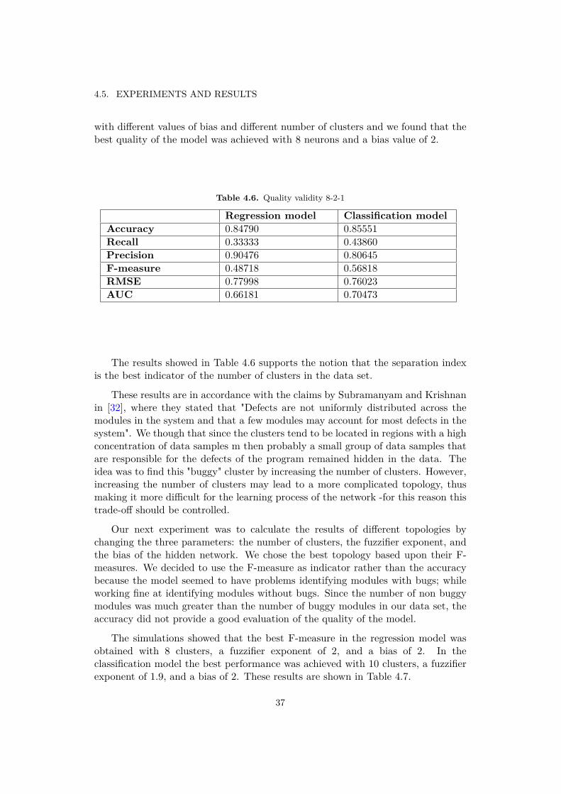
with different values of bias and different number of clusters and we found that thebest quality of the model was achieved with 8 neurons and a bias value of 2.

Table 4.6. Quality validity 8-2-1


The results showed in Table 4.6 supports the notion that the separation indexis the best indicator of the number of clusters in the data set.

These results are in accordance with the claims by Subramanyam and Krishnanin [32], where they stated that "Defects are not uniformly distributed across themodules in the system and that a few modules may account for most defects in thesystem". We though that since the clusters tend to be located in regions with a highconcentration of data samples m then probably a small group of data samples thatare responsible for the defects of the program remained hidden in the data. Theidea was to find this "buggy" cluster by increasing the number of clusters. However,increasing the number of clusters may lead to a more complicated topology, thusmaking it more difficult for the learning process of the network -for this reason thistrade-off should be controlled.

Our next experiment was to calculate the results of different topologies bychanging the three parameters: the number of clusters, the fuzzifier exponent, andthe bias of the hidden network. We chose the best topology based upon their F-measures. We decided to use the F-measure as indicator rather than the accuracybecause the model seemed to have problems identifying modules with bugs; whileworking fine at identifying modules without bugs. Since the number of non buggymodules was much greater than the number of buggy modules in our data set, theaccuracy did not provide a good evaluation of the quality of the model.

The simulations showed that the best F-measure in the regression model wasobtained with 8 clusters, a fuzzifier exponent of 2, and a bias of 2. In theclassification model the best performance was achieved with 10 clusters, a fuzzifierexponent of 1.9, and a bias of 2. These results are shown in Table 4.7.

37


Table 4.7. Quality validity


Figures 4.2 and 4.3 show the ROC curve of the regression and the classificationmodel respectively.

Figure 4.2. ROC curve of the regression model 10-8-1

38


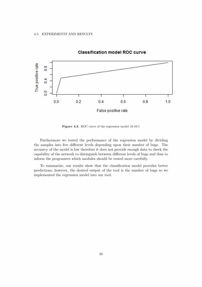
Figure 4.3. ROC curve of the regression model 10-10-1

Furthermore we tested the performance of the regression model by dividingthe samples into five different levels depending upon their number of bugs. Theaccuarcy of the model is low therefore it does not provide enough data to check thecapability of the network to distinguish between different levels of bugs and thus toinform the programers which modules should be tested more carefully.

To summarize, our results show that the classification model provides betterpredictions; however, the desired output of the tool is the number of bugs so weimplemented the regression model into our tool.

39

Chapter 5

Design of the tool

The tool has been developed using bash scripting. The tool implements twofunctionalities:

Predicts the number of bugs of a given file or files of a directory, and

Implements a new neuro-fuzzy hybrid model and trains it.

The prediction mode uses the default regression model to estimate the predic-tions. The results can be given on a per file or per module basis. In both cases theresults are generated for every module/file with the files ranked in descendent orderof their number of bugs.

The training mode allows the user to implement the neuro-fuzzy hybrid model.In this new implementation the data set and the parameters (in this case the numberof clusters, fuzzifier exponent, and bias of the hidden neurons) can be changed. Theparameters can be defined by the user or be selected by the program. After training,the tool compares the new results with the original results and asks for the user’sconfirmation to save the network which achieves the best performance..

Further explanation of the commands used to run the tool can be found inAppendix A.

The requirements to run the tool can be found in Appendix B.

5.1. Analysis of the tool

We analyzed some of the features of the tool:

User-friendly

After show a demo of the tool to its future users the tool seemed to be easy to

41

CHAPTER 5. DESIGN OF THE TOOL

use and the output information easy to understand.

Operation

The time execution of the program in both modes (prediction mode and trainingmode) depends upon the data set desired to be parsed. In our case, when we use asinput data the whole project (1755 modules), it took to the program half an hourto estimate the predictions and more than one hour to train the network. The mainreason of this waste of time was the necessity of the CCCC program to have all thefiles in the same directory (at the same level) to parse them properly as a whole.Therefore, the improvement of the execution time is related with the improvementin the features of the CCCC program. Regarding the operation of the program anyproblem was found in any of the modes.

Error handling

The tool implements error handling. The user is informed when the commandsused are not properly typed and when there have been a problem during theexecution of the program. In this case, an error message is displayed in the shellgiving some information about where the problem occurred.

Portability

The tool could be incorporated as part of the c-make of any project. In ourparticular case the tool was incorporated in the c-make of the project in such waythat users had the option to run it in background mode every time they compiledthe project. When our tool was enabled all the code of the project was parsed andpredictions were estimated. The increment of time while making the project wasconsiderable, for that reason, by default, the tool is disables in the c-make. Futurework out of the scope of this project is to integrate the tool as part of Jenkins.Thus, the project is monitored and the predictions are estimated every day.

Adaptability

The tool has been developed by using license free or open source programs. Ituses the R tool and the CCCC program and it can be adapted without problemsto new versions of both programs as far as the R version support the requiredpackages and the CCCC program does not change completely their output XMLreport. Furthermore, it would be easy to add more metrics and/or new programminglanguages if the CCCC supports them.

42

Chapter 6

Conclusion

In this thesis project we have written a program to predict the number of bugsin source code. The program is based on a neuro-fuzzy hybrid model created from afirst stage clustering, followed by a Radial Basis Function Neural Network. However,the program does not achieve high accuracy due to the lack of independent samplesin the data set. Neuro-fuzzy hybrid models are very dependent upon the data setused to train them. Thus, large data sets across different source code should be usedto get a high level of accuracy in predicting bugs. The user must use the functionsof the program to simulate a new model and train it with different and larger datasets.

Regarding the experiments done within this thesis project, the results haveshown that incorrect choices in the number of clusters leads to large changes in theresults of the RBFNN. Bad initializations in the clustering process and hence in theneural network can easily lead to sub-optimal clustering and thus in not accuratepredictions. The sensitivity to initialization becomes acute when the data set is notlarge enough.

It should also be mention that in our experiments the partition index seemedto be the best indicator of number of clusters in the data set was supported by theneural network results. In addition, should be mention that our experiments showthat fuzzifier values close to 2 lead to better predictions. This value is the mostfrequent value used in previous studies.

To conclude, experiments showed that classification models produce betterpredictions than regression models. This is because of the accuracy required fromthe network to predict buggy/non buggy models in these two different types ofmodels.

43

Chapter 7

Future work

This chapter suggests future work to improve upon the results shown thisthesis project. Section 7.1 focuses on the improvements associated with theimplementation of the model used to relate metrics with bugs. Section 7.2 focuseson the possible improvements of the tool.

7.1. Model improvements

The first task that should be done is to use larger data sets across differentsets of source code to train the neuro-fuzzy hybrid model of the tool. Larger andmore independent training data sets would lead to a more accurate tool with betterabilities to detect error-prone source code.

Regarding the software metrics more metrics can be added, or the existentones can be changed since the right combination of metrics could make a hugeimprovement to the early prediction of bugs. It is important to adapt the softwaremetrics to the programming language so they can better define the quality of thecode. Programs which estimate the value of the software metrics with greateraccuracy could be used also to improve the accuracy of the model.

It would also a major improvement to modify the methodology followed whenreporting bugs. In the tool we assign different bugs to the modules as a function ofthe bugs that we extract from the files, consequently, the number of bugs assignedto each module is overestimated. Thus, we propose to report the bugs indicatingthe exact modules that were necessary to modify in order to fix the bugs.

Regarding the neuro-fuzzy hybrid model, it would be interesting to have aneural network able to detect, as the Gustafson-Kessel Algorithm, different shapesof clusters in the data set. These shapes remain unknown and we forced them tobe gather in circular clusters.

45

CHAPTER 7. FUTURE WORK

Lastly, future studies in early bug prediction may use genetic algorithms.Genetic algorithms can be used to set the weights of the links in a fixed architectureand to define the number of hidden neurons. Moreover, genetic algorithms have amore interesting application from this thesis project’s perspective: we could selectthe training data of the data set which leads to the best learning by the neuralnetwork. These genetic algorithms discard non useful information and keep onlythe representative samples.

7.2. Tool improvements

The tool has multiple potential improvements that could lead make it a moreuseful and complete program. We propose three major improvements:

The tool could be implemented to run on different platforms (such as Mi-crosoft’s Windows).

The tool could have a more intuitive user interface.

The tool could be improved in order to predict bugs in different programminglanguages.

Furthermore, it would be a major improvement to adapt the program to predictbugs in C language since there are many repositories with large data sets that canbe used to train the model. It would be easy for users to find an open source codefor which all the bugs have been previously reported. Thus, a better analysis of theaccuracy of the model could be carried out.

46

Chapter 8

Required reflections

Nowadays companies and customers demand an improvement in the quality ofthe software products. This thesis project has shown that bug prediction is a feasiblegoal that would improve the quality of the software and decrease the costs of thesoftware development process. In addition, bug prediction would also decrease thecost of the customers since they may skip the costs of their own testing and thecost of the maintenance of the product. Therefore, the tool developed in this thesisproject must be used to improve the process of detecting and correcting bugs in thesoftware development process.

Further development of this tool may provide

more efficient developers since programmers using this tool will learn the leasterror-prone programming styles; and with

more efficient development process since the location of the bugs will be givenas soon as the code is written. This tool together with the new agile methodswill allow the user to resolved the bugs very fast.

47

Bibliography

[1] S.N. Ahsan and F. Wotawa. Fault prediction capability of program file’s logical-coupling metrics. In Software Measurement, 2011 Joint Conference of the 21stInt’l Workshop on and 6th Int’l Conference on Software Process and ProductMeasurement (IWSM-MENSURA), pages 257 –262, Nov. 2011.

[2] Robert Babuska. Fuzzy clustering with applications in pattern recognition anddata-driven modeling. Technical report, Delft Center for Systems and Control,Delft University of Technology, Netherlands.

[3] V.R. Basili, L.C. Briand, and W.L. Melo. A validation of object-oriented designmetrics as quality indicators. Software Engineering, IEEE Transactions on,22(10):751 –761, Oct. 1996.

[4] Christoph Bergmeir and José M. Benítez. Neural networks in R using thestuttgart neural network simulator: RSNNS. Journal of Statistical Software,46(7):1–26, 2012.

[5] Bergmeir C. and BenÃŋtez J. RSNNS: Neural networks in r using thestuttgart neural network simulator (snns). http://cran.r-project.org/web/packages/RSNNS/index.html, 2012.

[6] S.R. Chidamber and C.F. Kemerer. A metrics suite for object oriented design.Software Engineering, IEEE Transactions on, 20(6):476 –493, Jun. 1994.

[7] Dimitrios Siganos Christos Stergiou. Neural networks. http://www.doc.ic.ac.uk/~nd/surprise_96/journal/vol4/cs11/report.html#Asimpleneuron. Accessed:1 December 2012.

[8] C. Couto, C. Silva, M.T. Valente, R. Bigonha, and N. Anquetil. Uncoveringcausal relationships between software metrics and bugs. In Software Mainte-nance and Reengineering (CSMR), 2012 16th European Conference on, pages223 –232, March 2012.

49

http://cran.r-project.org/web/packages/RSNNS/index.html

http://cran.r-project.org/web/packages/RSNNS/index.html

http://www.doc.ic.ac.uk/~nd/surprise_96/journal/vol4/cs11/report.html#A simple neuron



BIBLIOGRAPHY

[9] M. D’Ambros, M. Lanza, and R. Robbes. An extensive comparison of bugprediction approaches. In 7th IEEE Working Conference on Mining SoftwareRepositories (MSR), 2010, pages 31 –41, May 2010.

[10] S. Dick and A. Kandel. Fuzzy clustering of software metrics. In Fuzzy Systems,2003. FUZZ ’03. The 12th IEEE International Conference on, volume 1, pages642 – 647 vol.1, May 2003.

[11] M. Dixon. An objective measure of code quality. Technical report, Energygroup, 2008.

[12] C. Frelicot, L. Mascarilla, and M. Beithier. A new cluster validity index forfuzzy clustering based on combination of dual triples. In IEEE InternationalConference on Fuzzy Systems, 2006, pages 42 –47, 0-0 2006.

[13] Qiang Gan and C.J. Harris. A hybrid learning scheme combining em andmasmod algorithms for fuzzy local linearization modeling. Neural Networks,IEEE Transactions on, 12(1):43 –53, Jan. 2001.

[14] Carlos Gershenson. Artificial neural networks for beginners. http://arxiv.org/ftp/cs/papers/0308/0308031.pdf, 2003. Accessed:1 December 2012.

[15] S. Henry and D. Kafura. Software structure metrics based on information flow.Software Engineering, IEEE Transactions on, SE-7(5):510 – 518, Sept. 1981.

[16] Tu Honglei, Sun Wei, and Zhang Yanan. The research on software metricsand software complexity metrics. In Computer Science-Technology and Appli-cations, 2009. IFCSTA ’09. International Forum on, volume 1, pages 131 –136,Dec. 2009.

[17] J.C.Bezdek. Fuzzy Mathematics in Pattern Classification. PhD thesis, AppliedMath. Center, Cornell University, Ithaca, 1973.

[18] Cong Jin, Shu-Wei Jin, Jun-Min Ye, and Qing-Guo Zhang. Quality predictionmodel of object-oriented software system using computational intelligence. InPower Electronics and Intelligent Transportation System (PEITS), 2009 2ndInternational Conference on, volume 2, pages 120 –123, Dec. 2009.

[19] Uzay Kaymak and Magne Setnes. Extended fuzzy clustering algorithms. ERIMreport series Research in Management, Erasmus nRS-2000-5 1 -LIS, ResearchInstitute of Management, Erasmus University Rotterdam, Netherlands, Nov.2000.

[20] R. Krishnapuram and Jongwoo Kim. A note on the gustafson-kessel andadaptive fuzzy clustering algorithms. IEEE Transactions on Fuzzy Systems,7(4):453 –461, aug 1999.

50

http://arxiv.org/ftp/cs/papers/0308/0308031.pdf

http://arxiv.org/ftp/cs/papers/0308/0308031.pdf

[21] Hua Jie Lee, Lee Naish, and K. Ramamohanarao. Study of the relationship ofbug consistency with respect to performance of spectra metrics. In 2nd IEEEInternational Conference on Computer Science and Information Technology,2009. ICCSIT 2009., pages 501 –508, Aug. 2009.

[22] J.A. Leonard and M.A. Kramer. Radial basis function networks for classifyingprocess faults. Control Systems, IEEE, 11(3):31 –38, April 1991.

[23] Tim Littlefair. CCCC: C and C++ code counter. http://cccc.sourceforge.net/, 1997. Accessed:1 December 2012.

[24] Michele Lanza Marco D’Ambros and Romain Robbes. Evaluating defectprediction approaches: a benchmark and an extensive comparison. EmpiricalSoftware Engineering (EMSE), 17(4):531–577, 2012.

[25] T.J. McCabe. A complexity measure. Software Engineering, IEEE Transac-tions on, SE-2(4):308 – 320, Dec. 1976.

[26] R Core Team. R: A Language and Environment for Statistical Computing. RFoundation for Statistical Computing, Vienna, Austria, 2012. ISBN 3-900051-07-0.

[27] J. Ratzinger, H. Gall, and M. Pinzger. Quality assessment based on attributeseries of software evolution. In Reverse Engineering, 2007. WCRE 2007. 14thWorking Conference on, pages 80 –89, Oct. 2007.

[28] R. Rojas. Neural networks, a systematic introduction. Technical report,Springer-Verlag, Berlin, New-York, 1996.

[29] A.R. Gray S.G. MacDonell. A comparison of modeling techniques for soft-ware development effort prediction. In International Conference on NeuralInformation Processing and Intelligent Information Systems, pages 869–872.Springer-Verlag, 1997.

[30] P. Singh and S. Verma. Empirical investigation of fault prediction capabilityof object oriented metrics of open source software. In Computer Science andSoftware Engineering (JCSSE), 2012 International Joint Conference on, pages323 –327, 30 May 2012-1 June 2012 2012.

[31] Ian Sommerville. Software Engineering. Addison Wesley, 7 edition, May 2004.

[32] R. Subramanyam and M.S. Krishnan. Empirical analysis of ck metrics forobject-oriented design complexity: implications for software defects. SoftwareEngineering, IEEE Transactions on, 29(4):297 – 310, april 2003.

51

http://cccc.sourceforge.net/

http://cccc.sourceforge.net/

BIBLIOGRAPHY

[33] Iris Vessey and Ron Weber. Research on structured programming: Anempiricist’s evaluation. Software Engineering, IEEE Transactions on, SE-10(4):397 –407, July 1984.

[34] Yongxue Wang and Yan Shang. Fuzzy clustering rbf neural network appliedto signal processing of the imaging detection. In Measuring Technologyand Mechatronics Automation (ICMTMA), 2010 International Conference on,volume 2, pages 321 –324, March 2010.

[35] E.J. Weyuker. Evaluating software complexity measures. Software Engineering,IEEE Transactions on, 14(9):1357 –1365, Sep 1988.

[36] K. Woods and K.W. Bowyer. Generating roc curves for artificial neuralnetworks. Medical Imaging, IEEE Transactions on, 16(3):329 –337, June 1997.

[37] X.l. Xie and G. Beni. A validity measure for fuzzy clustering. IEEE Trans-actions on Pattern Analysis and Machine Intelligence, 13(8):841 –847, Aug1991.

[38] Miin-Shen Yang and Kuo-Lung Wu. A new validity index for fuzzy clustering.In The 10th IEEE International Conference on Fuzzy Systems, volume 1, pages89 –92, 2001.

[39] Andreas Zell. SNNS Stuttgart Neural Network Simulator User Manual, Version4.2. University of Stuttgart and WSI, University of Tubinga, 1998.

52

Appendix A

Sinopsis of the tool

It is possible to specify a path to a file/directory if the user wants to run theprogram over one file or one directory of the project, rather than over the wholeproject.

For prediction:

1 >ZMetriX -p [-file/- module ] [path to file/ directory ] (path togit repository )

Options:

-file: shows the results by file in PredictedBugreportbyfile

-module: shows the results by module in PredictedBugreportbymodule

For training:

1 >ZMetriX -t [- default ] [path to file/ directory ] (path to gitrepository )

Options:

-default: The program defines the number of clusters, fuzzifier exponent, andbias of the neuro-fuzzy hybrid model. If the default mode is not selected, theprogram will ask the user to define these parameters.

After the model is implemented the program compares the original model withthis new model. The program recommends saving the best network (based uponthe value of its F-measure), but the user must decide which model they want tokeep. If "yes" is typed, then the original network is deleted and the new network issaved as the new default regression model. If "no" is typed then the new network is

53

APPENDIX A. SINOPSIS OF THE TOOL

deleted.

To run the program in training mode is necessary to have a file called Bugs.txtwith the actual number of bugs associated with each module of the data set. If theuser does not have this file, they should run first the command:

1 >sh Extractbugs (path to git repository )

54

Appendix B

Requirements of the tool

The requirements for the correct operation of the program are:

The CCCC program should be installed

The R program should be installed with the following packages: "e1071","RSN"NS", "ROCR". The minimum version required is 2.15.

Xmlstarlet should be installed on Linux.

CCCC program should be installed

The distributed version control system where the bugs are reported must beGIT and bugs should be reported with the word "artif".

55

Appendix C

Introducción

Actualmente, la industria de la telecomunicación es un mercado abierto enel que numerosas empresas compiten por el liderazgo; es por tanto un requisitoobligatorio para las compañías que compiten en este tipo de mercados ofrecer unaalta calidad y confiabilidad en sus productos para mantener su posición dentrodel mismo. Más específicamente, este objetivo es obligatorio para las compañíasdedicadas al desarrollo de software debido a que un software de alta calidad reducela cantidad de recursos necesarios para su mantenimiento y ayuda a la compañía aobtener una porción mayor del mercado. Consecuentemente, managers relacionadoscon el desarrollo y el mantenimiento de software han decidido apostar por mejorarel proceso de desarrollo del software en pos de obtener una mayor calidad en susoftware con un coste más reducido [10].

Este ciclo de vida o proceso del desarrollo de software es emulado cada vezque una compañía decide crear un nuevo producto software o mejorar uno yaexistente. Este proceso consiste, de al menos, los siguientes pasos: especificación,diseño, desarrollo o implementación, prueba o validación, documentación, entrega,y mantenimiento [31]. El modelo en cascada de este proceso puede verse en laFigura 1.1. Por simplicidad en este projecto se explica el modelo en casacada,pero el alcance de este proyecto es también aplicable a otros modelos de desarrollosoftware. Estos pasos son:

Especificación Los clientes determinan los requerimientos y el propósito delsoftware

Diseño Los responsables del proyecto en conjunto con los programadores definenla metodología y el diseño del producto.

Desarrollo Los programadores desarrollan el nuevo software.

Prueba Los programas son probados en busca de cualquier posible error que puedaproducir fallos en el sistema. Esta etapa suele ser la que más recursos consume.

57

APPENDIX C. INTRODUCCIÓN

Documentación y Mantenimiento En esta etapa los programas son documen-tados y comienza el proceso de mantenimiento. En este proceso se supervisa elcorrecto funcionamiento del producto; cuando es necesario se corrigen erroreso/y se implementan mejoras.

C.1. Descripción del problema

El proceso de prueba está diseñado para asegurar la calidad de los productossoftware, pero es el proceso que más recursos consume en términos de tiempo,esfuerzo, y coste. Esta actividad supone entre un 50 y un 70 por ciento de los costestotales del proyecto [21]. Los errores humanos y los malentendidos entre el hombre yla máquina son comunes en la programación. Estos errores son producidos durantela implementación del código, pero no son descubiertos hasta que éste es probado.Una vez descubiertos, estos errores obligan a los desarrolladores a implementarcódigo nuevo o a rescribir parte del código, lo que puede a su vez introducir nuevoserrores convirtiendo este proceso en un proceso exponencial. El esfuerzo necesariopara corregir estos errores mientras el código está siendo implementado es muchomenor que el necesario para corregirlos cuando el producto está siendo probado; enel peor de los casos son los usuarios finales lo que detectan estos errores en tiempode ejecución. En muchos casos los defectos introducidos por estos errores no sepueden resolver y es necesaria la creación de una nueva versión del código paraeliminarlos. En ambos escenarios, la compañía gasta una gran cantidad de recursosen corregir los errores. Es fácil comprobar por tanto que cuánto antes un errores encontrado y corregido, menor es el coste total. Así mismo, incrementaría lasatisfacción de los consumidores y su confianza en la empresa y sus productos [18].En consecuencia numerosas compañías han decidido invertir en nuevas formas dedetección y corrección de errores en las primeras etapas del proceso de desarrollo[18], por ejemplo el adoptando métodos ágiles, haciendo uso de especificacionesformales u otras técnicas.

C.2. Objetivos

El objetivo principal de este proyecto es mejorar la calidad del software. Parallevar a cabo esta mejora, este proyecto se centrará en la predicción de la presenciade errores en las primeras etapas del proceso de desarrollo. Así, en este proyectose creará une herramienta capaz de predecir la existencia de errores en un códigosoftware basándose en sus métricas. Esta predicción facilitará la detección de losmódulos más propensos a tener errores en un programa mientras este está siendodesarrollado. Más específicamente, esta herramienta permitirá al usuario a:

corregir errores durante la etapa de desarrollo que de otra forma no serían

58

C.3. ESTRUCTURA

encontrados hasta la etapa de pruebas (esto sería posible mediante la refac-torización del código fuente);

conocer que módulos deben ser probados más cuidadosamente y cuales no; y

aprender que estilos de programación son menos propensos a errores a travésde los resultados de la herramienta.

C.3. Estructura

El capítulo 1 introduce los objetivos y la motivación del proyecto.

El capítulo 2 presenta los antecedentes y conocimientos necesarios para la lecturay entendimiento del proyecto. Este capítulo comienza con algunas definicionesbásicas de la programación orientada a objetos, continúa con la descripción delas métricas del software más utilizadas, y concluye con una descripción de algunosde los modelos de regresión más empleados centrándose en los modelos híbridosneuro-difusos, en las redes neuronales y en las técnicas de agrupamiento.

El capítulo 3 ofrece una visión general del modelo utilizado para la creaciónde la herramienta. Este capítulo comienza con una breve explicación de lasespecificaciones de la herramienta y continúa con la selección de los programas,técnicas, y modelos empleados en este proyecto para relacionar las métricas delsoftware y los errores.

El capítulo 4 describe en detalle la implementación del modelo híbrido neuro-difuso. El capítulo finaliza analizando los resultados del modelo y su calidad.

El capítulo 5 explica las funcionalidades de la herramienta y los resultados deluso de esta herramienta.

El capítulo 6 presenta las conclusiones del proyecto.

El capítulo 7 propone trabajo futuro para mejorar la herramienta.

Finalmente los apéndices A y B contienen información más detallada de laherramienta.

59

Appendix D

Conclusiones

En este proyecto se ha creado un programa basado en un modelo híbrido neuro-difuso que predice el número de errores de un código fuente. Este modelo estácompuesto por una etapa de agrupación seguida de una red neuronal de funciónde base radial por lo que es muy dependiente del conjunto de datos usado paraentrenarlo. Por ello, grandes bancos de datos provenientes de diferentes códigosfuente deben ser utilizados para alcanzar un elevado nivel de precisión. Debido a lafalta de muestras independientes en el conjunto de datos utilizado en este proyecto,el resultado del análisis del programa ha concluido que este no ha alcanzado altaprecisión en sus predicciones. Se deja por tanto en manos del usuario, utilizar lasfunciones de la herramienta para simular un nuevo modelo y entrenarlo con grandesconjuntos de datos.

En cuanto a los experimentos realizados en este proyecto, los resultados hanmostrado que una elección incorrecta del número de grupos en el proceso deagrupación produce grandes alteraciones en los resultados de la RBFNN, siendoel índice de partición el mejor indicador de este valor. A su vez, estos resultadosmostraron que valores del exponente de difusión cercanos a 2 (que como se viopreviamente es valor más utilizado en estudios previos) resultaban en mejorespredicciones. Malas inicializaciones en el proceso de agrupación, y por tanto, enla red neuronal, conducen a agrupaciones sub-óptimas y a predicciones poco fiables.Esta sensibilidad a la inicialización se ve incrementada cuando el conjunto de datosno es lo suficientemente grande.

Por último, los experimentos han mostrado que los modelos de clasificaciónhacen mejores predicciones que los modelos de regresión debido a la precisiónrequerida para clasificar una muestra como errónea o no en ambos casos.

61

Appendix E

Presupuesto1) Ejecución Material

Compra de ordenador personal (Software incluido) 1.000 e

Material de oficina 150 e

2) Honorarios Proyecto1200 horas /150e la hora 18.000 e

3) Material fungibleGastos de impresión 280 e

Encuadernación 200 e

4) Subtotal del presupuestoSubtotal Presupuesto 19.980 e

5) I.V.A. aplicable21% Subtotal Presupuesto 4.195,8 e

6) Total presupuestoTotal Presupuesto 24.175,8 e

Madrid, 3 de Abril del 2013

El Ingeniero Jefe de Proyecto

Fdo.: Cecilia Rodríguez Martínez

Ingeniero Superior de Telecomunicación

63

Appendix F

Pliego de condiciones

Este documento contiene las condiciones legales que guiarán la realización, eneste proyecto, de un estudio de la calidad del software. En lo que sigue, se supondráque el proyecto ha sido encargado por una empresa cliente a una empresa consultoracon la finalidad de realizar dicho estudio. Dicha empresa ha debido desarrollar unalínea de investigación con objeto de elaborar el proyecto. Esta línea de investigación,junto con el posterior desarrollo de los programas está amparada por las condicionesparticulares del siguiente pliego.

Supuesto que la utilización industrial de los métodos recogidos en el presenteproyecto ha sido decidida por parte de la empresa cliente o de otras, la obra arealizar se regulará por las siguientes:

Condiciones generales.

1. La modalidad de contratación será el concurso. La adjudicación se hará,por tanto, a la proposición más favorable sin atender exclusivamente al valoreconómico, dependiendo de las mayores garantías ofrecidas. La empresa quesomete el proyecto a concurso se reserva el derecho a declararlo desierto.

2. El montaje y mecanización completa de los equipos que intervengan serárealizado totalmente por la empresa licitadora.

3. En la oferta, se hará constar el precio total por el que se compromete a realizarla obra y el tanto por ciento de baja que supone este precio en relación conun importe límite si este se hubiera fijado.

4. La obra se realizará bajo la dirección técnica de un Ingeniero Superior deTelecomunicación, auxiliado por el número de Ingenieros Técnicos y Progra-madores que se estime preciso para el desarrollo de la misma.

5. Aparte del Ingeniero Director, el contratista tendrá derecho a contratar alresto del personal, pudiendo ceder esta prerrogativa a favor del Ingeniero

65

APPENDIX F. PLIEGO DE CONDICIONES

Director, quien no estará obligado a aceptarla.

6. El contratista tiene derecho a sacar copias a su costa de los planos, pliego decondiciones y presupuestos. El Ingeniero autor del proyecto autorizará con sufirma las copias solicitadas por el contratista después de confrontarlas.

7. Se abonará al contratista la obra que realmente ejecute con sujeción al proyectoque sirvió de base para la contratación, a las modificaciones autorizadas porla superioridad o a las órdenes que con arreglo a sus facultades le hayancomunicado por escrito al Ingeniero Director de obras siempre que dicha obrase haya ajustado a los preceptos de los pliegos de condiciones, con arreglo alos cuales, se harán las modificaciones y la valoración de las diversas unidadessin que el importe total pueda exceder de los presupuestos aprobados. Porconsiguiente, el número de unidades que se consignan en el proyecto o en elpresupuesto, no podrá servirle de fundamento para entablar reclamaciones deninguna clase, salvo en los casos de rescisión.

8. Tanto en las certificaciones de obras como en la liquidación final, se abonaránlos trabajos realizados por el contratista a los precios de ejecución materialque figuran en el presupuesto para cada unidad de la obra.

9. Si excepcionalmente se hubiera ejecutado algún trabajo que no se ajustase alas condiciones de la contrata pero que sin embargo es admisible a juicio delIngeniero Director de obras, se dará conocimiento a la Dirección, proponiendoa la vez la rebaja de precios que el Ingeniero estime justa y si la Direcciónresolviera aceptar la obra, quedará el contratista obligado a conformarse conla rebaja acordada.

10. Cuando se juzgue necesario emplear materiales o ejecutar obras que no figurenen el presupuesto de la contrata, se evaluará su importe a los precios asignadosa otras obras o materiales análogos si los hubiere y cuando no, se discutiránentre el Ingeniero Director y el contratista, sometiéndolos a la aprobación dela Dirección. Los nuevos precios convenidos por uno u otro procedimiento, sesujetarán siempre al establecido en el punto anterior.

11. Cuando el contratista, con autorización del Ingeniero Director de obras,emplee materiales de calidad más elevada o de mayores dimensiones de loestipulado en el proyecto, o sustituya una clase de fabricación por otra quetenga asignado mayor precio o ejecute con mayores dimensiones cualquier otraparte de las obras, o en general, introduzca en ellas cualquier modificaciónque sea beneficiosa a juicio del Ingeniero Director de obras, no tendrá derechosin embargo, sino a lo que le correspondería si hubiera realizado la obra conestricta sujeción a lo proyectado y contratado.

12. Las cantidades calculadas para obras accesorias, aunque figuren por partidaalzada en el presupuesto final (general), no serán abonadas sino a los preciosde la contrata, según las condiciones de la misma y los proyectos particulares

66

que para ellas se formen, o en su defecto, por lo que resulte de su mediciónfinal.

13. El contratista queda obligado a abonar al Ingeniero autor del proyecto ydirector de obras así como a los Ingenieros Técnicos, el importe de sus respec-tivos honorarios facultativos por formación del proyecto, dirección técnica yadministracion en su caso, con arreglo a las tarifas y honorarios vigentes.

14. Concluida la ejecución de la obra, será reconocida por el Ingeniero Directorque a tal efecto designe la empresa.

15. La garantía definitiva será del 4% del presupuesto y la provisional del 2%.

16. La forma de pago será por certificaciones mensuales de la obra ejecutada, deacuerdo con los precios del presupuesto, deducida la baja si la hubiera.

17. La fecha de comienzo de las obras será a partir de los 15 días naturales delreplanteo oficial de las mismas y la definitiva, al año de haber ejecutado laprovisional, procediéndose si no existe reclamación alguna, a la reclamaciónde la fianza.

18. Si el contratista al efectuar el replanteo, observase algún error en el proyecto,deberá comunicarlo en el plazo de quince días al Ingeniero Director de obras,pues transcurrido ese plazo será responsable de la exactitud del proyecto.

19. El contratista está obligado a designar una persona responsable que se enten-derá con el Ingeniero Director de obras, o con el delegado que éste designe,para todo relacionado con ella. Al ser el Ingeniero Director de obras el queinterpreta el proyecto, el contratista deberá consultarle cualquier duda quesurja en su realización.

20. Durante la realización de la obra, se girarán visitas de inspección por personalfacultativo de la empresa cliente, para hacer las comprobaciones que se creanoportunas. Es obligación del contratista, la conservación de la obra yaejecutada hasta la recepción de la misma, por lo que el deterioro parcial ototal de ella, aunque sea por agentes atmosféricos u otras causas, deberá serreparado o reconstruido por su cuenta.

21. El contratista, deberá realizar la obra en el plazo mencionado a partir de lafecha del contrato, incurriendo en multa, por retraso de la ejecución siempreque éste no sea debido a causas de fuerza mayor. A la terminación de laobra, se hará una recepción provisional previo reconocimiento y examen porla dirección técnica, el depositario de efectos, el interventor y el jefe de servicioo un representante, estampando su conformidad el contratista.

22. Hecha la recepción provisional, se certificará al contratista el resto de la obra,reservándose la administración el importe de los gastos de conservación de lamisma hasta su recepción definitiva y la fianza durante el tiempo señalado

67

APPENDIX F. PLIEGO DE CONDICIONES

como plazo de garantía. La recepción definitiva se hará en las mismascondiciones que la provisional, extendiéndose el acta correspondiente. ElDirector Técnico propondrá a la Junta Económica la devolución de la fianzaal contratista de acuerdo con las condiciones económicas legales establecidas.

23. Las tarifas para la determinación de honorarios, reguladas por orden dela Presidencia del Gobierno el 19 de Octubre de 1961, se aplicarán sobreel denominado en la actualidad "Presupuesto de Ejecución de Contrata" yanteriormente llamado "Presupuesto de Ejecución Material" que hoy designaotro concepto.

Condiciones particulares.

La empresa consultora, que ha desarrollado el presente proyecto, lo entregará ala empresa cliente bajo las condiciones generales ya formuladas, debiendo añadirselas siguientes condiciones particulares:

1. La propiedad intelectual de los procesos descritos y analizados en el presentetrabajo, pertenece por entero a la empresa consultora representada por elIngeniero Director del Proyecto.

2. La empresa consultora se reserva el derecho a la utilización total o parcialde los resultados de la investigación realizada para desarrollar el siguienteproyecto, bien para su publicación o bien para su uso en trabajos o proyectosposteriores, para la misma empresa cliente o para otra.

3. Cualquier tipo de reproducción aparte de las reseñadas en las condicionesgenerales, bien sea para uso particular de la empresa cliente, o para cualquierotra aplicación, contará con autorización expresa y por escrito del IngenieroDirector del Proyecto, que actuará en representación de la empresa consultora.

4. En la autorización se ha de hacer constar la aplicación a que se destinan susreproducciones así como su cantidad.

5. En todas las reproducciones se indicará su procedencia, explicitando el nombredel proyecto, nombre del Ingeniero Director y de la empresa consultora.

6. Si el proyecto pasa la etapa de desarrollo, cualquier modificación que se realicesobre él, deberá ser notificada al Ingeniero Director del Proyecto y a criteriode éste, la empresa consultora decidirá aceptar o no la modificación propuesta.

7. Si la modificación se acepta, la empresa consultora se hará responsable almismo nivel que el proyecto inicial del que resulta el añadirla.

8. Si la modificación no es aceptada, por el contrario, la empresa consultoradeclinará toda responsabilidad que se derive de la aplicación o influencia dela misma.

9. Si la empresa cliente decide desarrollar industrialmente uno o varios productos

68

en los que resulte parcial o totalmente aplicable el estudio de este proyecto,deberá comunicarlo a la empresa consultora.

10. La empresa consultora no se responsabiliza de los efectos laterales que sepuedan producir en el momento en que se utilice la herramienta objeto delpresente proyecto para la realización de otras aplicaciones.

11. La empresa consultora tendrá prioridad respecto a otras en la elaboración delos proyectos auxiliares que fuese necesario desarrollar para dicha aplicaciónindustrial, siempre que no haga explícita renuncia a este hecho. En este caso,deberá autorizar expresamente los proyectos presentados por otros.

12. El Ingeniero Director del presente proyecto, será el responsable de la direcciónde la aplicación industrial siempre que la empresa consultora lo estimeoportuno. En caso contrario, la persona designada deberá contar con laautorización del mismo, quien delegará en él las responsabilidades que ostente.

69

Documents

UNIVERSIDAD AUT“NOMA DE MADRID PROYECTO FIN DE CARRERA Software quality studies