Journal of Monetary Economics 18 (1986) 49-75. North-Holland

UNIVARIATE DETRENDING METHODS WITH STOCHASTIC TRENDS

Mark W. WATSON* Harvard Uniuersiry and NBER, Cambridge, MA 02138, USA

This paper discusses detrending economic time series, when the trend is modelled as a stochastic process. It considers unobserved components models in which the observed series is decomposed into a trend (a random walk with drift) and a residual stationary component. Optimal detrending methods are discussed, as well as problems associated with using these detrended data in regression models. The methods are applied to three time series: GNP, disposable income, and consumption expenditures. The detrended data are used to test a version of the Life Cycle consumption model.

1. Introduction

Most macroeconomic time series exhibit a clear tendency to grow over time and can be characterized as ‘trending’. The statistical theory underlying most modem time series analysis relies on the assumption of covariance stationar- ity, an assumption that is clearly violated by most macroeconomic time series. In applied econometric work it is usually assumed that this statistical theory can be applied to deviations of the observed time series from their trend value. Since it is often the case that these deviations or economic fluctuations are of primary interest, modem time series techniques are often applied to ‘de- trended’ economic time series.

Much recent work has been devoted to issues involving trends or long-run components in economic series. Some of this work has devoted itself to the proper characterization of ‘trends’ in economic data. A notable’contribution on this topic is the paper by Nelson and Plosser (1982) which considers the use of deterministic and stochastic trends. Other work [e.g., Nelson and Kang (1981, 1984)] has been concerned with the econometric consequences of misspecification in the model for the trend component. Still more work has addressed the issue of detecting long-run relations [e.g. Geweke (1983)] or incorporating long-run relationships in short-run dynamic relations [e.g., the work on ‘error correction models’ begun in Davidson et al. (1978) and the

*I would like to thank Andy Abel, Olivier Blanchard, Rob Engle, Charles Plosser, Charles Nelson, and Jim Stock for useful comments and discussions. I would also like to thank the National Science Foundation for financial support.

0304-3923/86/$3.5001986, Elsevier Science Publishers B.V. (North-Holland)

50 M. W. Watson, Detrending methods with stochastic trena!s

co-integrated processes introduced in Granger (1983) and discussed further in Engle and Granger (1984)].

Research concerning the proper characterization of long-run trend behavior in economic time series is important for a variety of reasons. First, the work of Nelson and Kang and others shows that misspecification in the model for the trend can seriously affect the estimated dynamics in an econometric model. Proper estimation of these dynamic relations is important if they are to be used to test modem theories of economic behavior. These theories put very tight restrictions on the dynamic interrelations between economic variables. h&specification of trend components will often lead the analyst to incorrect inferences concerning the validity of these theories. The proper specification of long-run relations is also critical for long-term forecasting.

This paper makes two points. The first point concerns the theory of stochastic detrending, and the second concerns its empirical implementation. We first propose a method for removing stochastic trends from economic time series. The method is similar to the one originally proposed by Beveridge and Nelson (1981), but differs in one important respect. The problem is cast in an unobserved components framework, in which the trend is modelled as a random walk with drift, and the residual ‘cyclical’ component is modelled as a covariance stationary process. This framework allows us to discuss and con- struct optimal detrending methods. One of the optimal methods corresponds to the (negative of the) Beveridge and Nelson transitory component. Our theoretical work shows that, in principle, our unobserved components (UC)’ representation of the process describing the data will give exactly the same results as the usual ARIMA representation. That is, both models imply exactly the same long-run behavior of the data.

The second point of this paper is that estimated ARIMA and UC models imply very different long-run behavior of economic time series. For example, we estimate UC and ARIMA models for post-war US GNP. Both models yield essentially identical values of the likelihood function and short-run forecasts. However, estimated long-run behavior of the models is quite differ- ent. The ARIMA model implies that an innovation of one unit in GNP is expected to eventually increase the level of GNP by 1.68 units, the UC model implies that the same innovation will eventually increase GNP by only 0.57 units. These results suggest that it is a dangerous practice to use the estimated time series models such as ARIMA or UC models to make inferences about long-run characteristics of economic time series.

The paper is organized as follows. The next section specifies the model for the observed series, the trend component, and the residual ‘cyclical’ compo-

‘Unobserved component models of the kind used in this paper have been advocated in Harvey

and Todd (1983) and more recently in Harvey (1985). These two references contain excellent discussions of the similarities and differences between dynamic behavior of models parameteked as parsimonious ARIMA models and those parameterized as UC models.

M. W. Watson, Derrending methodr with stocktic trends 51

nent. We begin with a general ARIMA formulation for the observed series and describe how the stochastic process can be ‘factored’ into the two processes for the components. Identification issues are also addressed in this section. Section 3 discusses methods for estimating and eliminating the stochastic trends. The properties of the detrended series are addressed, and special attention is paid to the use of these series in constructing econometric models. The final two sections contain empirical examples. Three post-war US macroeconomic time series - GNP, disposable income, and consumption of non-durables - are analysed. Section 4 looks at each of these series in isolation, and presents and compares various estimates of the detrended series. Section 5 uses the data for non-durable consumption and disposable income to test the ‘consumption follows a random walk’ implication of one version of the life cycle consump- tion model. The final section contains a short summary and some concluding remarks.

2. The model

This section will introduce three models that additively decompose an observed time series, x,, into a trend and cyclical component. Each of these models will assume, or imply, that the change in x, is a covariance.stationary process. We begin with the Wold representation for the change in x,, which we write as

(1 -B)x,=6+8”(B)ef, var(e:)=c&, P-1)

where IF(B) is a polynomial in the backshift operator B, and e: is white noise. The assumption that (1 - B)x, is stationary is appropriate for most non-seasonal macroeconomic time series. Seasonal series often require a differencing operator of the form (1 - B”) where s is the seasonal span (12 for monthly, 4 for quarterly, etc.). Our assumption is not adequate to handle these series, and therefore, we are assuming that the series are non-seasonal.

The representation for the level of the series x, that we consider in this paper is

x,=r,+c,, (2.2)

where

7, = 6 + 7r-1 + e:, var( er) = CT,‘,, (2.3)

and (c,, e;) is a jointly stationary process. A variety of specific assumptions about this process will be discussed below. The component 7, corresponds to the trend component in the variable x,; the ‘detrending’ will attempt to

52 hi. W. Watson, Detrending methods with stochastic trends

eliminate this component. Eq. (2.3) represents this trend as a random walk with drift, which can be viewed as a flexible linear trend. The linear trend is a special case of (2.3) and corresponds to the restriction u,‘, = 0. The forecast function of (2.3) is linear with a constant slope of 6 and a level that varies with the realization of e;. More general formulations are certainly possible. Harvey and Todd (1983) consider a model in which the drift term, a,, evolves as a random walk. This allows the slope as well as the level of the forecast function of 71 to vary through time. This formulation implies that x, must be dif- ferenced twice to induce stationarity, and therefore is ruled out by our assumption that (1 - B)x, is stationary.

To complete the specification of the model we must list our assumptions concerning the covariance properties of c, and the cross-covariances between c, and e;. We consider three sets of assumptions. The assumptions will differ in the way that c, and e:-k are correlated. We consider each model in turn:

Model I

In this model the component c, evolves independently of the 7, component, and follows the process

c, = t3’(B)e;, (2.4.1)

where ef and eymk are uncorrelated for all k. The parameters of the UC model given by (2.2), (2.3), and (2.4.1) are econometrically identifiable. To see this, equate the representations for (1 - B)x, corresponding to (2.1) and the UC model given in (2.2), (2.3), and (2.4.1). This implies

Br(B)e:=e’+(l-B)B’(B)ef,

so that

[P(l) I’r& = o-,“,. 0.5)

The coefficients in P(B) can be found by forming the factorization of

ex(Z)eqZ-1)u,2,-u,2,= (1 -z)(l -z-‘)e~(z)e=(z-l)u~~, (2.6)

subject to the usual identifying normalizations [e.g., ~9: = 1 and the roots of e=(z) are on or outside the unit circle].

Eq. (2.6) can be used to show that (2.2)-(2.4.1) place testable restrictions on the x, process given in (2.1). To see this, set z = e-“‘, so that the right-hand side of (2.6) is the spectrum of (1 - B)c,. Since the spectrum is non-negative, the left-hand side of (2.6) must be non-negative for all o. This implies that

M. W. Watson, Detrending methods with stochastic trends 53

6x(e-i~)6~Y(eiw)u~x 2 u,‘, for all w, with equality guaranteed at w = 0 by (2.5). We conclude that the spectrum of (1 - B)x,, 6x(e-i0)6x(eiw)u$, has a global minimum at w = 0. Only processes with this feature can be represented by Model 1. [As discussed in Nelson and Plosser (1981), this rules out many common processes such as the ARIMA (l,l,O) with positive autoregressive coefficient.] The restrictiveness of this assumption will be investigated em- pirically for three macroeconomic time series in section 4.

Mast of the discussion in the remainder of the paper will be devoted to Model 1. The restrictiveness of the model, however, suggests that other models are needed if the UC model is to be useful in describing all models of the form given in (2.1). Because of this we briefly discuss two other models. These differ from Model 1 in the assumptions they make about the covariance between c, and e;-k. The first of these is:

Model 2

The model for c, is

c,= fl’(B)e:, (2.4.2)

where B’(B) is a one-sided polynomial in the backshift operator. In this model, the innovations in the trend and cyclical components are perfectly correlated. The advantage of this model is that there is a one-to-one corre- spondence between models of the form (2.1) and models characterized by (2.2), (2.3), and (2.4.2). This implies that the parameters of the UC formula- tion (2.3) and (2.4.2) are econometrically identiable, and that unlike Model 1, this UC formulation places no constraints on the model (2.1). [A proof of this assertion can be found in an earlier version of this paper, Watson (1985).]

The perfect correlation between the innovations in the components is an assumption that some might find objectionable on a priori grounds. Some correlation is needed, however, to give the UC model enough flexibility to capture all of the dynamic behavior possible in the model (2.1). Our final model is a mix of Models 1 and 2, in which the c, and r, are partially correlated.

Model 3

The component c, is represented as

c,=f(B)ef+f(B)e;, (2.4.3)

where $f(B) and v(B) are one-sided polynomials in B. This model can be viewed as a mixture of Models 1 and 2. Since both of those models are individually identifiable, Model 3 is not.

54 M. W. Watson, Detrending method with stochastic trends

3. Estimation issues

The models presented in the last section suggest that ‘detrending’ should be viewed as a method for estimating and removing the component 7, from the observed series x,. If we denote the estimated trend by r,, then the detrended series is given by t, = x, - +,. Different detrending methods correspond to different methods for estimating 7. A variety of criteria can be used to choose among competing estimation methods. We will consider linear minimum mean square error (LMSE) estimators constructed using information sets X,h = (x0, Xl, * * - > xh). We concentrate on these estimators for a variety of reasons. In addition to the usual reasons, including ease of computation and optimality for quadratic loss, the use of LMSE estimators guarantee certain orthogonality properties involving the estimation errors r, - +, = 2, - c,. These properties play a key role in the formation of instrumental variable estimators that are discussed below. We concentrate on a univariate information set for computa- tional ease. In general, multivariate methods will produce more accurate estimates. The univariate methods considered in this paper can serve’ as a benchmark to measure the marginal gains from considering more general, multivariate models.

We will discuss detrending in the context of the general model - Model 3. The results for Model 1 can be found by setting v(B) = 0 and ec( B) = @(B), and the results for Model 2 can be found by setting $I’( B) = 0 and P(B) = 4’(B). A convenient starting point for the discussion is the LMSE of using the information set ( . . . ,x-i, x0, xi,. . . ). In this case the standard Wiener filter for stationary processes [see, e.g., Whittle (1963)] can be extended to this non- stationary case [see Bell (1984)] to yield

T,= V(B)X,= C”ixy-iS (3.1)

where the coefficients in the two-sided polynomial V(B) can be found from

v(x) = ee’7[1+ (1 -z-‘)$7(z-‘)] [P(z)P(z-i)c&] -l.

We denote E(w,]X,h) by w,,,, for any variable w (where E is used to denote the projection operator). From eq. (3.1),

(3.3)

so that the estimates of the trend using the information set X,h can be formed from the Wiener filter with unknown values of x replaced by forecasts or backcasts constructed from the set Xi.

The form of the tllter V(B) given in (3.2) makes it clear that the LMSE estimate depends on I#J’( z). Different V(B) polynomials will be associated with

h4. W. Watson, Detrending methods with stochastic trenak 55

Models 1, 2, and 3, so that different LMSE estimates of c, will be constructed. Eq. (3.2) makes it clear, however, that the difference arises from the way in which future data is used in the construction of r,,,,. All models produce the identical values of r,,,, for h < t. This is easily demonstrated. From (2.2),

x,/h = ‘t/h + ‘t/h-

For h I t,

7,-k k/h = ‘t/h +k6 for k=1,2,...,

so that

*,+k/h - ks = rt/h + Ct+k/hm

Since all of the models imply that c, is stationary (with mean zero),

lim( k + m) c,+k,,, = 0,

so that

lim(k+ @+,+k,h- ktJ] =T,//,e

This result shows that, in principle, the estimates c,,, (which will be called the filtered estimates) can be formed without access to any specialized soft- ware. To calculate the filtered estimates one merely constructs an ARIMA model for x, and then forecasts the series (less the deterministic increases kt3) into the distant future. This forecast corresponds to the filtered estimate, r,,t, and c,,, = x, - r,,,. This estimate of a permanent component was first sug- gested by Beveridge and Nelson (1981) in their permanent/transitory decom- position of economic time series. They define their transitory component as T/t -x,= -c t,,, in the notation above. This discussion shows that their estimate of the permanent component corresponds to an optimal one-sided estimator for the trend in the models under consideration in this paper.

While the optimal filtered estimate c,,, is identified - is not model-depen- dent - its precision is not identified. That is, the mean square of (c, - c,,,) will depend on the assumed model. If Model 2 is used to describe the decomposition of the data, then c,,, = c,, so that the mean square error is zero. For the other models, x, is made up of both noises e7 and ec so that it is impossible to perfectly disentangle r, and c, when only their sum, x,, is observed. Since the Models 1, 2, and 3 are observationally equivalent, the mean square of (c, - c,,,) is not identi8ed.

The remainder of this section will focus on the use of estimated values of c, in linear regression models. Replacing c, by c,,, in regression models leads to

56 M. W. Watson, Detrending methods with stochastic trends

problems similar to those in the classic errors-in-variables model. As the examples below will demonstrate, OLS estimates of regression coefficients will quite often be inconsistent.

We will begin our discussion by writing the orthogonal decomposition of c, as

c~ = ct/h + ‘t/h 1

where a,,,, is the signal extraction error that arises from the use of informa- tion set X,h. Ordinary least square regression estimates rely on sample covari- antes between observable variables, and the consistency of OLS estimates follows from the consistency of these sample covariances. Consider then the covariance between an arbitrary variable w and c. From the decomposition of c, we have

cov( w,c,) = cov( w,cIlh) + cov( w,a,/h).

The cov( w,c,) will be consistently estimated by the sample covariance between w, and c,/h if cov(w,a,,,) = 0. In general this will not be true, so that cov(w,c,) f cov(w,c,/h). Recall, however, that a,/,, is a projection error, so that it is uncorrelated with linear combinations of data in X,h. By constructing w, as a linear combination of the elements in Xi, we can .guarantee that cov(w,c,) = cov(w,c,,,). We will use this fact in construction of instrumental variable estimators. It will be convenient to discuss a variety of estimation issues in the context of some specific models.

The tirst model has current and lagged values of c, as independent variables, so that

k

y, = c q-i&+ z;v + t,, i-.1

where z, is a i vector of unobserved variables, and we will assume (without loss of generality) that .& is white noise. We can rewrite this model in terms of unobserved variables as

k

YI’ C ct-i/h?i + z;Y + 5, + fl a,-i/h& i-l i-l

= IfI ‘t-i/hfli + z;y + U,s i-l

M. W. Watson, Detrending methoak with stochastic trends 57

where u, is the composite error term (&+ ~~~,~,-~,,,/3~). The unknown parameters Ply /$, . . . , Bk ad yl, - . . , yj will be consistently estimated by OLS if the regressors c,-~,,, and t, are uncorrelated with the error term u,. This may not be true for a variety of reasons.

Two sources of correlation are immediately apparent. First, consider the correlation between c,- i,h and [,. In many models it will be reasonable to assume that 5, is uncorrelated with current and lagged values of c,, but unreasonable to assume that 5, is uncorrelated with future values of c,. (Correlation between [, and c,+~ will exist if there is feedback from y, to c,.) But when h > t, c,-~,~ will contain future x,‘s, and therefore c,-~,,, will contain linear combinations of future c,‘s. This may induce a correlation between c,-~,~ and 6, even though c,-~ and & are uncorrelated. The second source of correlation between the regressors and the disturbance arises from the possible correlation between z, and u,+,,,. These variables will be correlated when z, contains useful information about c, not contained in XJ.

These problems can be circumvented by the use of instrumental variables. In particular, the variables in X6 can be used as instruments to estimate the model. When constructing instrumental variable estimates, it is useful to make use of the fact that, for h > t, c,,, = E(c,,,,IX$, so that IV estimates can be formed by regressing y, on the filtered values, c,,,, and i,, the fitted values from the regression of z, onto the set of instruments. Finally, it should be pointed out that the error terms, u,, may be serially correlated so that standard errors may have to be calculated using the procedures outlined in Cumby, Huizinga and Obstfeld (1983) or Hayashi and Sims (1983).

The second regression model that we consider is

k

Ct = 1 ct-ipi + z:y + Et* i-l

This model should be interpreted as the true generating equation for c,, so that 5, is uncorrelated with all variables dated t - 1 or earlier. Models 1-3 described in the last section can be viewed as reduced forms of this model, where the z,‘s have been solved out as in Zellner and Palm (1976). Writing the model in terms of observables, we have

Ct/h = i$l ‘t-i/hbi

k

+Z:Y +tt+ c at-i/h&-at/h i-l

k

= C Ct-i/hBi t- Z:y + Ut. i-l

58 M. W. Warson, Detrending methods with stochastic treno5

As in the previous model, the observed regressors c,-;,,, and z, may be correlated with the error term, u,, leading to inconsistency of the OLS estimates. When h r I, the estimates c,-~,,, contain future c,‘s and therefore will be correlated with 5,. The variables z, can be viewed as ‘causes’ of c, and will therefore contain useful information about the c’s, which is not contained in the univariate information set X,h. This will induce a correlation between z, and a,-i/h. Instrumental variables can again be used to estimate the model. The data in Xi-l are valid instruments.

In the discussion above, we replaced the true values of c,-~ by the estimates c,-~,,,. Since these estimates depend crucially on the model for c,, a useful alternative is to replace them by the estimates c,-~,,-~, which do not depend on the model assumed for c,. The see the implications of this procedure, rewrite the first regression example as

k k

y, = C C,-i/r-iSi + Z:Y - 5, + C a,-i/t-iSi-

i-l i-l

This differs from the formulation above in that each c,-~ is estimated using a different information set. Since cov(c,-i,,-ia,-j,,-j) # 0 for i >j, care must be taken in choosing instruments. Since Xi 3 XA-’ 3 . . . 3 XAmk, data in Ximk are valid instruments, and this set can be used.

Finally, it is important to keep in mind that the inconsistency in OLS estimates will depend on the magnitude of the error in the estimate of c,. When c, is estimated very precisely, the inconsistencies from OLS have no practical importance.

4. Univariate examples

In this section we will analyze three US macroeconomic time series - real GNP, real disposable income, and real consumption of non-durables. We begin by applying the univariate detrending methods outlined in the last section to the logs of these series, using quarterly data from 1949 through 1984. The estimated univariate models and corresponding trend and cyclical components will be discussed in this section. In the next section, we will investigate the relation between the cyclical components of disposable income and consumption using regression methods.

Two univariate models have been estimated for each series. The first is the usual ARIMA model. The second is an unobserved components (UC) model suggested by the independent trend/cycle decomposition in Model 1. For each time series, we will present and compare the models and their corresponding

M. W. Watson, Derrending methods with srochastic trends 59

trend/cycle decomposition. The analysis in the last section indicated that, given the Wold decomposition of the observed series, the optimal one-sided estimates of the components could be formed using any of the observationally equivalent representations of the data. In principle then, it shouldn’t matter whether we form the one-sided estimates from the ARIMA model or from the UC model. The results below show that, in practice, it matters a great deal which representation is used. This apparent contradiction arises from the fact that the Wold representation for the data is not known. The ARIMA model and the UC model correspond to different parsimonious approximations to the Wold representation. Given a finite amount of data is is very difficult to discriminate between these alternative representations for the data sets that we consider.

4.1. GNP

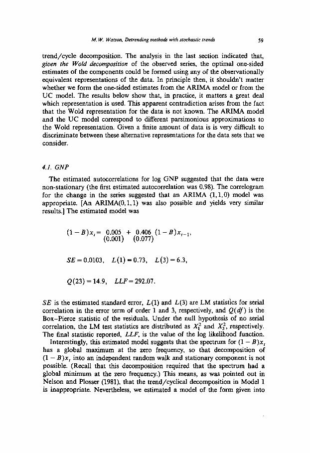
The estimated autocorrelations for log GNP suggested that the data were non-stationary (the first estimated autocorrelation was 0.98). The correlogram for the change in the series suggested that an ARIMA (1, 1,O) model was appropriate. [An ARIMA(O,l,l) was also possible and yields very similar results.] The estimated model was

(1 - B)x,= 0.005 + 0.406 (1 -@x,-r, (0.001) (0.077)

SE = 0.0103, L(1) = 0.73, L(3) = 6.3,

Q(23) = 14.9, LLF= 292.07.

SE is the estimated standard error, L(1) and L(3) are LM statistics for serial correlation in the error term of order 1 and 3, respectively, and Q(df) is the Box-Pierce statistic of the residuals. Under the null hypothesis of no serial correlation, the LM test statistics are distributed as Xiz and Xi, respectively. The final statistic reported, LLF, is the value of the log likelihood function.

Interestingly, this estimated model suggests that the spectrum for (1 - B)x, has a global maximum at the zero frequency, so that decomposition of (1 - B)x, into an independent random walk and stationary component is not possible. (Recall that this decomposition required that the spectrum had a global minimum at the zero frequency.) This means, as was pointed out in Nelson and Plosser (1981), that the trend/cyclical decomposition in Model 1 is inappropriate. Nevertheless, we estimated a model of the form given into

60 M. W. Watson, Detrending methods with stochastic trends

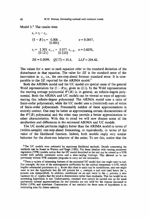
Model 1.’ The results were

x, = 7, - c,,

(l-l.+,= 0.008 , (0.001)

a=0.0057,

c,= (;:;;;,c,-~- O:;;:,c,e2, a=0.0076,

SE = 0.0099, Q(17) = 10.4, LLF= 294.42.

The values for u next to each equation refer to the standard deviation of the disturbance in that equation. The value for SE is the standard error of the innovation in x,, i.e., the one-step-ahead forecast standard error. It is com- parable to the SE reported for the ARIMA model.3

Both the ARIMA model and the UC model are special cases of the general Wold representation for (1 - B)x, given in (2.1). In the Wold representation the moving average polynomial F(B) is, in general, an infkite-degree poly- nomial. Both the ARIMA and UC models can be viewed as ways of approxi- mating this infinite-degree polynomial. The ARIMA model uses a ratio of finite-order polynomials, while the UC model uses a (restricted) sum of ratios of finite-order polynomials. Presumably neither of these approximations is entirely correct. One may be better at approximating certain characteristics of the 8”(B) polynomial and the other may provide a better approximation to other characteristics. With this in mind we will now discuss some of the similarities and differences in the estimated ARIMA and UC models.

The UC model performs slightly better than the ARIMA model in terms of (within-sample) one-step-ahead forecasting, or equivalently, in terms of the value of the likelihood function. Indeed, both models imply very similar behavior for the short-run behavior of the series. To see this, notice that the

*The UC models were estimated by maximum likelihood methods. Details concerning the methods can be found in Watson and Angle (1983). For those familiar with varying parameter regression (VPR) models, notice that the UC model described in the text can be viewed as a VPR model with serially correlated errors and a time-varying intercept. This allowed us to use previously written VPR computer programs to carry out the estimation.

3There a variety of interesting features of the estimated UC model that one might want to test. For example, the sum of the autoregressive coefficients for the cyclical component is 0.92, which implies substantial persistence in c,. Roots this close to unity can be troublesome, and one might want to test the hypothesis that the AR process for c, contains a unit root (and hence the c, process was misspecitied). In addition, conditional on no unit roots in the c, process, a zero variance for e: implies that the trend is deterministic rather than stochastic. This too would be an interesting hypothesis to test. Unfortunately, standard tests cannot be carried out, as the usual asymptotic normal approximations for test statistics are not valid for the reasons discussed in Fuller (1976) and elsewhere. Construction of test statistics for these sorts of hypotheses is an interesting area for future research.

M. W. Watson, Detrending metho& with stochastic trends 61

UC model implies that

(1 - 1.501B + OS77P)(l- B)x,

= (1 - 1.501B + 0.577B2)e:+ (1 - B)ef. (4-l)

By Granger’s Lemma the right-hand side of (4.1) can be represented as a MA(2) ,a.nd solving for the implied coefficients yields

(1 - 1.501B = 0.577P)(l- B)x,

= (1 - 1.144B + 0.189B2)a,, a,= 0.0099.

The autoregressive representation for the model is

(1 - 1.144B + 0.189B2)-‘(1 - 1.501B + 0.577B2)(1 - B)x,= ~1,.

Carrying out the polynomial division we have, approximately,

(1 - 0.36B- 0.05B2)(1- B)x,= a,,

which is very close to the estimated ARIMA model. While the short-run behavior of the UC and ARIMA models are very

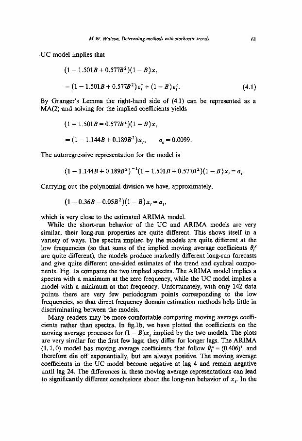
similar, their long-run properties are quite different. This shows itself in a variety of ways. The spectra implied by the models are quite different at the low frequencies (so that sums of the implied moving average coefficients 0: are quite different), the models produce markedly different long-run forecasts and give quite different one-sided estimates of the trend and cyclical compo- nents. Fig. la compares the two implied spectra. The ARIMA model implies a spectra with a maximum at the zero frequency, while the UC model implies a model with a minimum at that frequency. Unfortunately, with only 142 data points there are very few periodogram points corresponding to the low frequencies, so that direct frequency domain estimation methods help little in discriminating between the models.

Many readers may be more comfortable comparing moving average coeffi- cients rather than spectra. In fig.lb, we have plotted the coefficients on the moving average processes for (1 - B)x, implied by the two models. The plots are very similar for the first few lags; they differ for longer lags. The ARIMA (1, LO) model has moving average coefficients that follow 0: = (0.406)‘, and therefore die off exponentially, but are always positive. The moving average coefficients in the UC model become negative at lag 4 and remain negative until lag 24. The differences in these moving average representations can lead to significantly different conclusions about the long-run behavior of x,. In the

62 M. W. Watson, Detrending metho& with stochastic trends

I

I I I I I I I I s25l-l .5n .75rl II

Fig. la. Spectra for change in log GNP.

-0.50 1 I I I 0 I 5 IO 15 20

Lag

Fig. lb. Moving average coefficients for change in log GNP.

ARIMA model, for example, the sum of the moving average coefficients is 1.68, while in the UC model the sum of the moving average coefficients is 0.59. This means that using the AFUMA model, a one-unit innovation in x will eventually increase log GNP by 1.68, while in the UC model the same innovation is predicted to give rise to a 0.57 increase in GNP. Hypotheses concerning the effects of innovations on permanent income, defined as the discounted expected future sum of x,, are also quite different. The ARIMA model predicts an impact nearly three times as large, and therefore has fundamentally different implications for permanent income. [The relationship between the moving average coefficients in measured income and the perma- nent income hypothesis is discussed in Deaton (1985).]

M. W. Watson, Detrending methods with stochastic tren& 63

7.4 -

7.2-

7.0 -

,,,,,,,,,,,,,,,,,,,,,,,,,,,,,,,,C 51 53 55 57 59 61 63 65 67 69 71 73 75 77 79 81 83

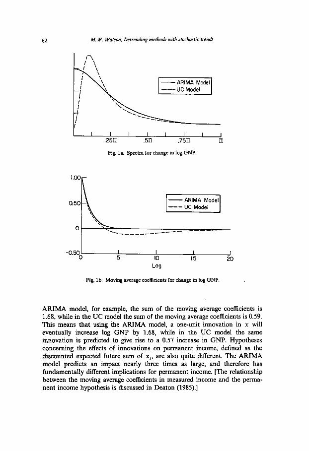
Fig. 2a. Trend decomposition for the log of GNP.

7.2 J . 6.8 - /pciJ 6.6- , / 6.4 11111,111,,,,,,,,,,, ,,,,,,,,,,,, I-

51 53 55 57 59 61 63 65 67 69 71 73 75 77 79 81 83

Fig. 2b. Trend decomposition for the log of GNP.

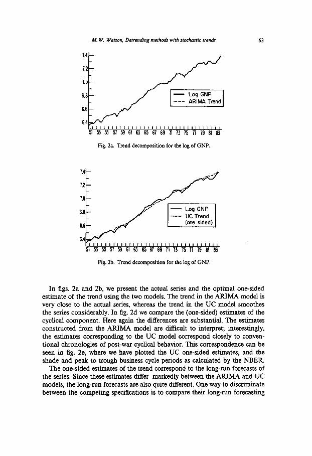
In figs. 2a and 2b, we present the actual series and the optimal one-sided estimate of the trend using the two models. The trend in the ARIMA model is very close to the actual series, whereas the trend in the UC model smoothes the series considerably. In fig. 2d we compare the (one-sided) estimates of the cyclical component. Here again the differences are substantial. The estimates constructed from the ARIMA model are difficult to interpret; interestingly, the estimates corresponding to the UC model correspond closely to conven- tional chronologies of post-war cyclical behavior. This correspondence can be seen in fig. 2e, where we have plotted the UC one-sided estimates, and the shade and peak to trough business cycle periods as calculated by the NBER.

The one-sided estimates of the trend correspond to the long-run forecasts of the series. Since these estimates differ markedly between the ARIMA and UC models, the long-run forecasts are also quite different. One way to discriminate between the competing specifications is to compare their long-run forecasting

64 M. W. Watson, Detrending methods with stochastic trends

7.2 t

7.0 7.0

6.6 6.6

6.6

6.4

Fig. 2c. Trend decomposition for the log of GNP.

- UC Cycle (one-sided)

n --- ARlMA Cycle

IIII1IIIIIIIIIIIIII1111 I,,,,,,,,, 51 53 55 57 59 61 63 65 67 69 71 73 75 77 79 81 8f

Fig. 2d. Cycle decomposition for the log of GNP.

.025

0 ES4 NEER Feak-

-.025

Fig. 2e. Cycle decomposition for the log of GNP.

M. W. Watson, Delrending methods with stochastic trends 65

l~~‘~~~~~~~~~~~~~~~~~1111111111111 51 53 55 57 59 61 63 65 67 69 71 73 75 77 79 81 63

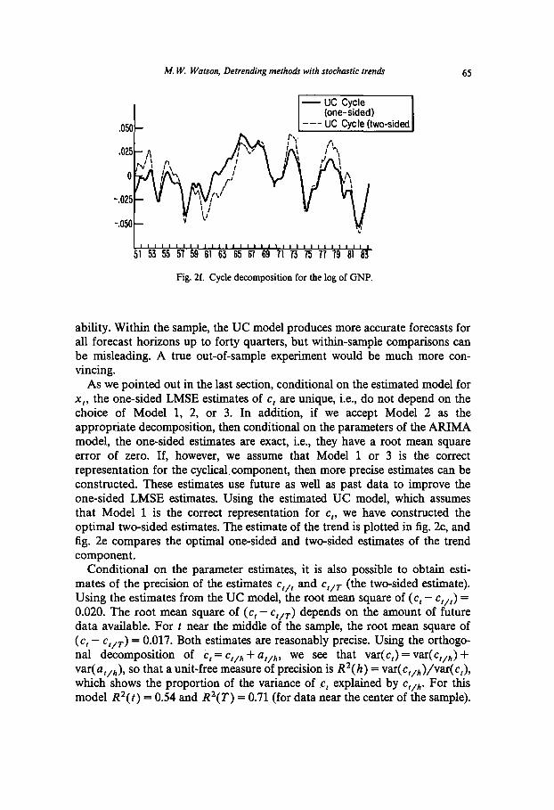
Fig. 2f. Cycle decomposition for the log of GNP.

ability. Within the sample, the UC model produces more accurate forecasts for all forecast horizons up to forty quarters, but within-sample comparisons can be misleading. A true out-of-sample experiment would be much more con- vincing.

As we pointed out in the last section, conditional on the estimated model for x,, the one-sided LMSE estimates of c, are unique, i.e., do not depend on the choice of Model 1, 2, or 3. In addition, if we accept Model 2 as the appropriate decomposition, then conditional on the parameters of the AIUMA model, the one-sided estimates are exact, i.e., they have a root mean square error of zero. If, however, we assume that Model 1 or 3 is the correct representation for the cyclicalcomponent, then more precise estimates can be constructed. These estimates use future as well as past data to improve the one-sided LMSE estimates. Using the estimated UC model, which assumes that Model 1 is the correct representation for c,, we have constructed the optimal two-sided estimates. The estimate of the trend is plotted in fig. 2c, and fig. 2e compares the optimal one-sided and two-sided estimates of the trend component.

Conditional on the parameter estimates, it is also possible to obtain esti- mates of the precision of the estimates c,,, and c,,r (the two-sided estimate). Using the estimates from the UC model, the root mean square of (c, - c,,,) = 0.020. The root mean square of (c, - c,,r) depends on the amount of future data available. For t near the middle of the sample, the root mean square of (‘t - ‘f/T ) = 0.017. Both estimates are reasonably precise. Using the orthogo- nal decomposition of C, = c,,,, + a,,,,, we see that var(c,) = var(c,,,) + var( u,,~), so that a unit-free measure of precision is R2( h) = var(c,,,)/var( c,), which shows the proportion of the variance of c, explained by c,,,,. For this model R2(t) = 0.54 and R2(T) = 0.71 (for data near the center of the sample).

66 M. W. Watson, Detrending methodr with stochastic treudr

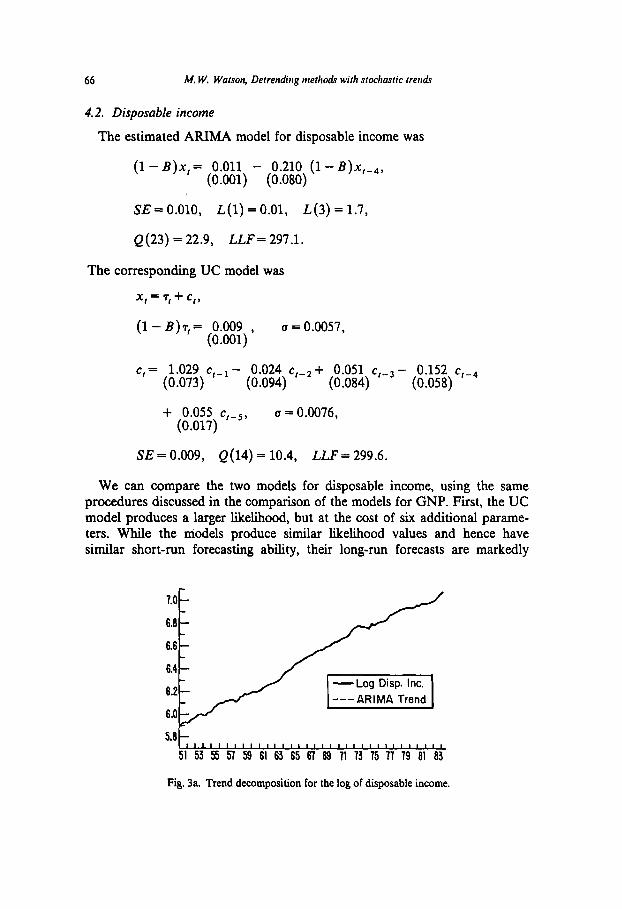
4.2. Disposable income

The estimated ARIMA model for disposable income was

(1 - B)x, = 0.011 - 0.210 (1 -B)x,+ (0.001) (0.080)

SE = 0.010, L(1) = 0.01, L(3) = 1.7,

Q(23) = 22.9, LLF= 297.1.

The corresponding UC model

x,=7,+c,,

(1 - B)7,= 0.009 , (0.001)

was

a=0.0057,

c,= 1.029 c,-r- (0.073)

0.024 c,m2+ 0.051 c,-~- 0.152 c,-4

(0.094) (0.084) (0.058)

+ 0.055 c,-j, (0.017)

a=0.0076,

SE = 0.009, Q(14) = 10.4, LLF = 299.6.

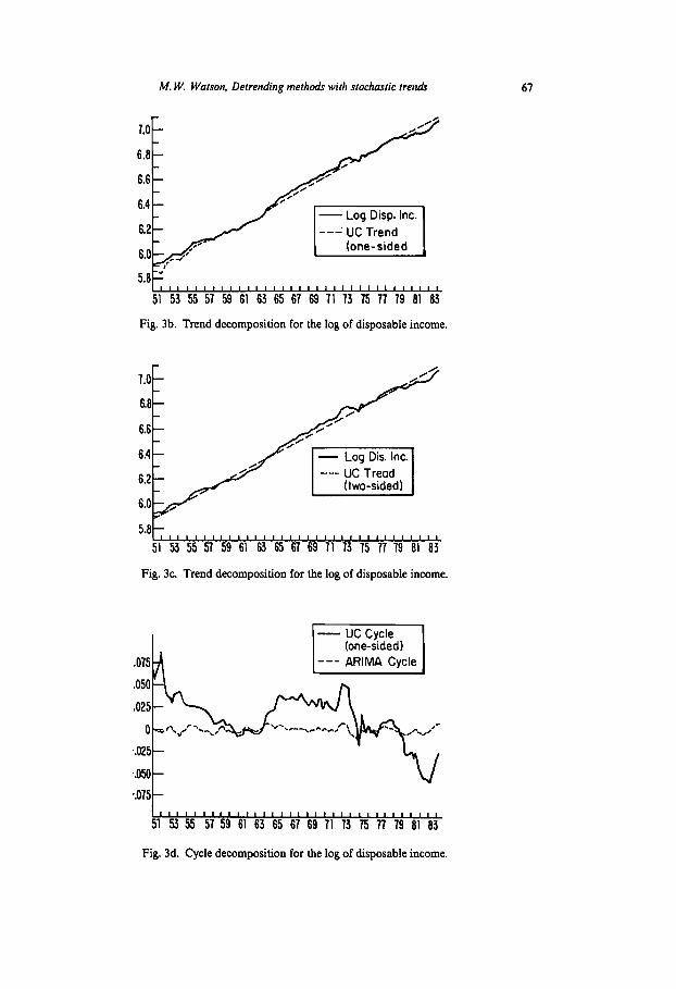
We can compare the two models for disposable income, using the same procedures discussed in the comparison of the models for GNP. First, the UC model produces a larger likelihood, but at the cost of six additional parame- ters. While the models produce similar likelihood values and hence have similar short-run forecasting ability, their long-run forecasts are markedly

7.0

6.8

6.6

6.4

6.2

5.8h , , , , , , , , , , , , , , , , , , , , , , , , , , , , , , , , 51 53 55 57 53 61 63 65 61 69 71 73 75 77 79 81 83

Fig. 3a. Trend decomposition for the log of disposable income.

M. W. Watson, Detrending methodr with stochastic fret&

7.0 - 7.0 -

6.6 - 6.6 -

6.6 - 6.6 -

---UC Trend ---UC Trend

5.6 .+, I1I1I11I1III11111111111111111111, I1I1I11I1III11111111111111111111,

51 51 53 53 55 55 57 57 59 59 61 61 63 63 65 65 67 67 69 69 71 71 73 73 75 75 77 77 79 79 61 61 63 63

Fig. 3b. Trend decomposition for the log of disposable income. Fig. 3b. Trend decomposition for the log of disposable income,

7.0

6.6

6.4 /G' I--

6.0 , b

5.6~,,,,,,,,,,,,,,,,,,,,,,,,,,,,,,,, 51 53 55 57 59 61 63 65 67 69 II 73 75 77 79 61 63

Fig. 3c. Trend decomposition for the log of disposable income.

.075

.050

$025

III1 I I IllI4 II II I II I1 I III II I,,,,,,,

51 53 55 57 59 61 63 65 67 69 71 73 75 77 79 61 63

Fig. 3d. Cycle decomposition for the log of disposable income.

M. W. Watson, Detrending methods with stochastic fret&

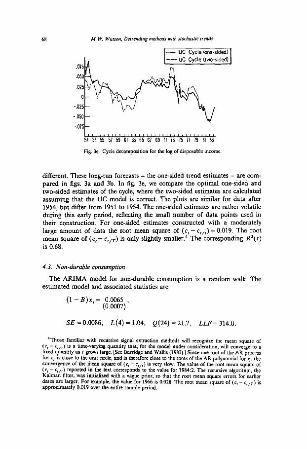
IIIILllltlllllllll1II1IIIII~II1I1 51 53 55 57 59 61 63 65 67 69 71 73 75 77 79 81 63

Fig. 3e. Cycle decomposition for the log of disposable income.

different. These long-run forecasts - the one-sided trend estimates - are com- pared in figs. 3a and 3b. In fig. 3e, we compare the optimal one-sided and two-sided estimates of the cycle, where the two-sided estimates are calculated assuming that the UC model is correct. The plots are similar for data after 1954, but differ from 1951 to 1954. The one-sided estimates are rather volatile during this early period, reflecting the small number of data points used in their construction. For one-sided estimates constructed with a moderately large amount of data the root mean square of (c, - c,,,) = 0.019. The root mean square of (c, - c,,,) is only slightly smaller.4 The corresponding R2(t) is 0.68.

4.3. Non-durable consumption

The ARIMA model for non-durable consumption is a random walk. The estimated model and associated statistics are

(1 - B)x,= 0.0065 , (0.0007)

SE = 0.0086, L(4) = 1.04, Q(24) = 21.7, LLF = 314.0.

4Those familiar with recursive signal extraction methods will recognize the mean square of (c, - c,,,) is a time-varying quantity that, for the model under consideration, will converge to a fixed quantity as t grows large. [See But-ridge and Wallis (1983).] Since one root of the AR process for c, is close to the unit circle, and is therefore close to the roots of the AR polynomial for 7,. the convergence of the mean square of (c, - c,,,) is very slow. The value of the root mean square of (c, - c,,,) reported in the text corresponds to the value for 1984:2. The recursive algorithm, the Kalman filter, was initialized with a vague prior, so that the root mean square errors for earlier dates are larger. For example. the value for 1966 is 0.028. The root mean square of (c, - c,,r) is approximately 0.019 over the entire sample period.

M. W. Watson, Detrending methods with stochastic trends 69

The estimated UC model was

x,=7,+c,,

(1 - B)T,= 0.0067 , (0.0003)

u = 0.0018,

c,= 0.940 C,-1, (0.036)

(I = 0.0082,

SE=0.0085, Q(20)= 14.9, LLF= 314.3.

The models are clearly very close to one another in terms of their one-step- ahead forecast ability and likelihood values. If we set the variance of the cyclical component to zero, the UC model implies that x, is a random walk, so that the random walk model is nested within the UC model. It is therefore possible, in principle, to test the competing models, using a likelihood ratio test. Unfortunately, the test is complicated by the fact that the AR coefficient in the model for c, is not identified under the random walk hypothesis, but it is identified in the more general model. This complicates the distribution of the likelihood ratio statistic; it will not have the usual asymptotic distribution. This problem has been discussed in detail in Watson and Engle (1985) and Davies (1977). They show that the correct (asymptotic) critical value for carrying out the test (using the square root of the likelihood ratio statistic) is bounded below by the critical value for the standard normal distribution. In this example, the square root of the likelihood ratio statistic is 0.77, which implies a lower bound of the (asymptotic) prob-value of 0.27. This suggests that the random walk hypothesis cannot be rejected at levels of 27% or less.

The examples in this section tell a consistent story. The short-run forecast- ing performance of the ARIMA and UC models are very similar. At longer forecast horizons, the forecasts from the models differ markedly. This dif- ference in the long-run properties of the estimated models, leads to very different estimates of the underlying trend components and cyclical compo- nents.

5. Regression examples

In this section we investigate the relationship between non-durable con- sumption expenditures and the cyclical component of disposable income. We

70 M. W. Watson, Detrending methodr with stochastic trends

test the proposition that the change in consumption from period t to t + 1 is uncorrelated with the cyclical component of disposable income dated t or earlier. The empirical validity of this proposition, first tested in Hall (1978), has been the subject of ongoing controversy. [See, for example, the papers by Flavin (1981), and Mankiw and Shapiro (1985).] The model that we consider implies that the change in log consumption from period t to period I + 1 should be unpredictable using information available at time t. We test this implication using the cyclical component of disposable income at time f. The importance of using a stationary variable (like the cyclical component of income) rather than a non-stationary variable (like the level of income) has been pointed out by Mankiw and Shapiro (1985). We begin by motivating the empirical specification that is used in this paper.

Assume that a consumer is choosing consumption to maximize a time-sep- arable utility function, subject to an intertemporal budget constraint, i.e., the consumer solves

ycyE( C (1 + S)-iuCC,+i)ll,), I i-0 (5.1)

subject to

E C (1 +r)-iC,+iII, i-0

where W, is wealth at time t (which includes the expected discounted value of future earning), 6 is a time-invariant subjective discount factor, I, is the information set at time t, and r is the constant one-period interest rate. The first-order conditions for utility maximization imply

E(Zt+,V,) = (1 + a)(1 + d-l, (5 4

where Z, + t = u’(C,+J/u’(C,) is the marginal rate of substitution for con- sumption between periods t and t + 1. An empirical specification follows from an assumption concerning the functional form of the utility function and the probability distribution for Z,. Here, we follow Hansen and Singleton (1983). Let z, = logZ,, and assume that z,+rl1, - N(p,, a*). The log normality of Z,+i implies that E(Z,+;II,) = exp(p,+ 0*/2). But (5.2) implies that E(Z,+,lI,) is constant, so that p, = ~1 for all r. If we now assume that u(C) is of the constant relative risk aversion form, so that u(C) = (1 - @-‘C’-fi, then z, = -&c,+r - c,), with c, = logC,. When c, is in the information set I,, this

hf. W. Warson, Deirending methodr with stochastic trends 71

implies

E(C r+1K) = c, + a5

with a = /3-‘[(02/2) + r - 61, so that

c I+1 =C,+"+e,+l, (5.3)

where e,,, is uncorrelated with information available at time t. We will test this proposition by investigating the correlation between (1 - B)c, and lagged values of the cyclical component of disposable income.

The analysis of the last section casts some light on the hypothesis embodied in (5.3). There we showed that the hypothesis that c, was a univariate random walk was consistent with the data. We calculated a ‘r-statistic’ associated with this hypothesis that had a value of 0.77. In this section we ask whether (1 - B)c, can be predicted by linear combinations of disposable income. The models that we will estimate in this section all have the form

(l-B)c,=a+p(B)y,“_,+e,, (5 -4

where y; is the cyclical component in disposable income, and p(B) is a one-sided polynomial in B. Under the assumption of the life cycle consump- tion model outlined above, p(B) = 0 for any choice of a (one-sided) poly- nomial. Since y,’ is not directly observed, the model (5.4) cannot be estimated by OLS. We will estimate the model using various proxies for the unobserved y,’ data. The sample period is 1954:l to 1984:2.’

Before proceeding to a test of this hypothesis using the data described in the last section, one issue concerning the data should be addressed. When this random walk hypothesis is tested using macro data, the consumption and income figures are usually deflated by population before the analysis begins. This expresses all variables in per-capita terms, so that the data are loosely consistent with a representative consumer notion. We have chosen not to follow this course. ,While we agree that this transformation is useful in principle, in practice it can lead to serious problems. These problems arise from the errors in the quarterly population series. While the underlying trend in the population estimate is probaly close to the trend in the true series, the quarter-to-quarter changes in the estimates series is, most likely, almost entirely noise. Indeed, over 50% of the sample variation in quarterly post-war population growth rates can be attributed to three large outliers in the data

5 We have started the sample period in 1954 to eliminate the observations in which the estimates y& are very imprecise. See the discussion in footnote 3.

12 M. W. Watson, Detrending methook with stochastic trends

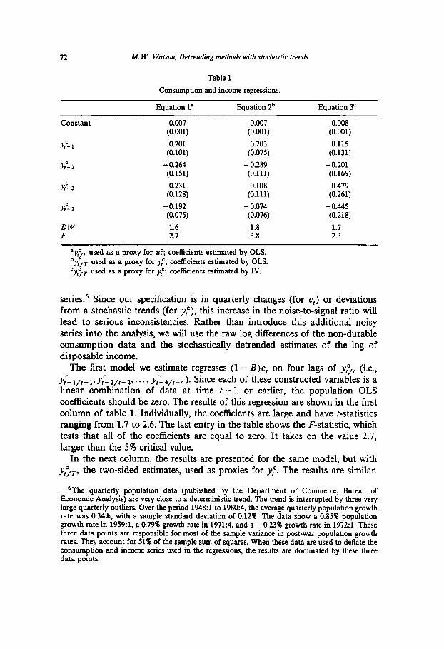
Table 1 Consumption and income regressions.

Equation 1’ Equation 2b Equation3'

constant 0.007 (0.001)

Yf=- I 0.201 (0.101)

u,=- 2 -0.264 (0.151)

I?-3 0.231 (0.128)

Y,'- 2 - 0.192 (0.075)

DW 1.6 F 2.7

0.007 0.008 (0.001) (0.001) 0.203 0.115

(0.075) (0.131) -0.289 - 0.201 (0.111) (0.169) 0.108 0.479

(0.111) (0.261)

-0.074 -0.445 (0.076) (0.218)

1.8 1.7 3.8 2.3

“y:,, used as a proxy for u:; coefficients estimated by OLS. by:/r used as a proxy for y,‘; coefficients estimated by OLS. ‘y& used as a proxy for y,‘; coefficients estimated by N.

series6 Since our specification is in quarterly changes (for c,) or deviations from a stochastic trends (for y:), this increase in the noise-to-signal ratio will lead to serious inconsistencies. Rather than introduce this additional noisy series into the analysis, we will use the raw log differences of the non-durable consumption data and the stochastically detrended estimates of the log of disposable income.

The first model we estimate regresses (1 - B)c, on four lags of yl’/, (i.e., Y,c-l,r-l~Y,c-Z,r-2,.-.~ y,!$,+,). Since each of these constructed variables is a linear combination of data at time t - 1 or earlier, the population OLS coefficients should be zero. The results of this regression are shown in the first column of table 1. Individually, the coefficients are large and have t-statistics ranging from 1.7 to 2.6. The last entry in the table shows the F-statistic, which tests that all of the coefficients are equal to zero. It takes on the value 2.7, larger than the 5% critical value.

In the next column, the results are presented for the same model, but with y&, the two-sided estimates, used as proxies for y,‘. The results are similar.

‘jThe quarterly population data (published by the Department of Commerce, Bureau of Economic Analysis) are very close to a deterministic trend. The trend is interrupted by three very huge quarterly outhers. Over the period 1948:l to 1980:4, the average quarterly population growth rate was 0.34% with a sample standard deviation of 0.12%. The data show a 0.85% population growth rate in 1959:i, a 0.79% growth rate in 1971:4, and a -0.23% growth rate in 1972:l. These three data points are responsible for most of the sample variance in post-war population growth rates. They account for 51% of the sample sum of squares. When these data are used to deflate the consumption and income series used in the regressions, the results are dominated by these three data points.

M. W. Watson, Detrending methods with stochastic trenak 13

The F-statistic is now 3.8, which is significant at any reasonable level. The results in this column, however, are perfectly consistent with the theory. Recall that the two-sided estimates contain future values of disposable income. Since future values of disposable income are not included in 1,-i, (1 - B)c, may be correlated with these variables. (Indeed we would expect innovations in consumption to be correlated with innovations in income.) If we proxy the components v,’ by the smoothed values and estimate the coefficients using data in 1,-i as instruments, then the coefficients should not be signi6cantly different from zero. The results of this exercise are shown in the third column. Only the last coefficient is now significant and the F-statistic has fallen to 2.3, significant at the 10% but not the 5% levels.

The results of this section suggest that aggregate post-war US data are not consistent with the life cycle model outlined above.

6. Concluding remarks

This paper was motivated by the desire for a flexible method to eliminate trends in economic time series. The method that was developed in this paper was predicated on the assumption that deterministic trend models were too rigid and not appropriate for most economic time series. The altema- tive - modelling economic time series as non-stationary stochastic processes of the ARIMA class - confused long-run and cyclical movements in the series. The useful, fictitious decomposition of a time series into trend and cyclical components could not be used when modelling series as ARIMA processes. The method described in this paper maintains the convenient trend/cycle decomposition, while allowing flexibility in the models for both of the compo- nents.

In addition to discussing a new method for ‘detrending’ economic time series, this paper makes an important empirical point. The paper compares two empirical approximations to the Wold representation for the changes in GNP, disposable income, and non-durable consumption expenditures. These two empirical approximations correspond to ARIMA and UC models. The models imply very similar short-run behavior for the series: the one-step-ahead forecasts from the models are nearly identical. The implied long-run behavior of the models are quite different. The UC models imply that innovations in the process have a much smaller impact on the long-run level of the series than is implied by the ARIMA model. It is very difficult to discriminate between the competing models on statistical grounds: their log-likelihoods are nearly identical. Since both competing models describe the data equally well, we are left with the conclusion that the data are not very informative about the long-run characteristics of the process. While this may seem to an obvious conclusion, one must keep in mind that very different conclusions would be reached using the implied large-sample confidence intervals constructed from

14 M. W. Watson, Detrending metho& with stochastic trends

either the UC or the ARIMA models. The difference arises because these large-sample confidence intervals are conditional on the specific parameteriza- tion of the Wold representation.

The paper also discussed the use of stochastically detrended data in the construction of econometric models. Here we demonstrated that care has to be taken to avoid inconsistencies arising from complications similar to errors- in-variables. Our empirical example investigated the relation between the change in consumption of non-durables and lags of the cyclical component of disposable income. Here we found a significant relation, which indicates that the simple life cycle model, with its maintained assumptions of constant discount rates, no liquidity constraints, and time-separable utility, is not consistent with aggregate post-war US data.

References

Bell, W., 1984, Signal extraction for nonstationary time series, Annals of Statistics 12, 646-684. Beveridge, S. and CR. Nelson, 1981, A new approach to decomposition of economic time series,

into permanent and transitory components with particular attention to measurement of the ‘business cycle’, Journal of Monetary Economics 7,151-174.

But-ridge, P. and K.F. Wallis, 1983, Signal extraction in nonstationary time series, University of Warwick working paper no. 234.

Cumby, R.E., J. Huizinga and M. Obstfeld, 1983, Two-step two-stage least squares estimation in models with rational expectations, Journal of Econometrics 21, 333-355.

Davidson, J.E.H., David F. Hendry, Frank Srba and Steven Yeo, 1978, Econometric modelling of the aggregate time-series relationship between consumer’s expenditure and income in the United Kingdom, Economic Journal 88,661-692.

Davies, R.B., 1977, Hypothesis testing when a nuissance parameter is present only under the alternative. Biometrika 64,247-254.

Deaton, Angus, 1985, Consumer behavior: Tests of the life cycle model, Invited paper delivered at the World Congress of the Econometric Society, Cambridge, MA.

Flavin, M., 1981, The adjustment of consumption to changing expectations about future income, Journal of Political Economy 89,974-1009.

Fuller, W.A., 1976, Introduction to statistical time series (Wiley, New York). Geweke, John, 1983, The supemeutrality of money in the United States: An interpretation of the

evidence, Carnegie-Mellon University discussion paper, May. Granger, C.W.J., 1983, Co-integrated and error-correcting models, UCSD discussion paper no.

83-13a. Granger, C.W.J. and R.F. Engle, 1984, Dynamic model specification with equilibrium constraints:

Co-integration and error-correction, UCSD discussion paper, Aug. Hansen, L. and K. Singleton, 1983, Stochastic consumption, risk aversion, and the temporal

behavior of asset returns, Journal of Political Economy 91,249-265. Hall, R.E., 1978, The stochastic implications of the life-cycle permanent income hypothesis:

Theorv and evidence. Journal of Political Economv 86.971-987. Harvey, AC., 1985, Trends and cycles in macroeconomic time series, Journal of Business and

Economic Statistics 3,216-227. Harvey, A.C. and P.H.J. Todd, 1983, Forecasting economic time series with structural and

Box-Jenkins models: A case study (with discussion), Journal of Business and Economic Statistics 1,299-315.

Hayashi, F. and C. Sims, 1983, Efficient estimation of time series models with predetermined, but not exogenous, instruments, Econometrica 51, 783-798.

Mankiw, N.G. and M.D. Shapiro, 1984, Trends, random walks, and tests of the permanent income hypothesis, Journal of Monetary Economics 16, 141-164.

M. W. Warson, Delrending methods with slochasric rren& 75

Nelson, C.R. and H. Kang, 1981, Spurious periodicity in inappropriately detrended time series, Econometrica 49, 741-751.

Nelson, C. R. and H. Kang, 1984, Pitfalls in the use of time as an explanatory variable in regression, Journal of Business and Economic Statistics 2, 73-82.

Nelson, C.R. and C.I. Plosser, 1981, Trends and random walks in macroeconomic time series: Some evidence and imphcations, Journal of Monetary Economics 10, 139-162.

Watson, M.W., 1985, Univariate detrending methods with stochastic trends, H.I.E.R. discussion paper no. 1158.

Watson, M.W. and R.F. Engle, 1983. Alternative algorithms for the estimation of dynamic factor, MIMIC, and varying coefficient regression models, Journal of Econometrics 23,485-500.

Watson, M.W. and R.F. Engle, 1985, Testing for regression coefficient stability with a stationary AR(l) alternative, Review of Economics and Statistics LXVII, 341-346.

Whittle, P., 1963, Prediction and regulation (English Universities Press, London). Zellner, A. and F. Palm, 1976, Time-series analysis and simultaneous equation econometric

models, Journal of Econometrics 2, 17-54.