Embed Size (px)
Citation preview

Submitted byAndreas Peter Pröll
Submitted atInstitute of StructuralLightweight Design
SupervisorUniv.-Prof. Dipl.-Ing. Dr.Martin Schagerl
Co-SupervisorAsst.-Prof. AdiAdumitroaie, Ph.D.Dipl.-Ing. LukasRetschitzegger
July 2017
JOHANNES KEPLERUNIVERSITY LINZAltenbergerstraße 694040 Linz, Österreichwww.jku.atDVR 0093696
Fatigue Damage Modelsfor LaminatedComposite Structures
Master’s Thesisto obtain the academic degree of
Diplom-Ingenieur
in the Master’s Program
Polymer Technologies and Science

Statutory Declaration i
Statutory DeclarationI hereby declare that the thesis submitted is my own unaided work, that I have not used other thanthe sources indicated, and that all direct and indirect sources are acknowledged as references. Thisprinted thesis is identical with the electronic version submitted.
place and date Signature

Abstract ii
AbstractMany cyclic loaded structures show damage after a certain number of cycles even though the max-imum stress in a cycle is far below static strength. This phenomenon is called fatigue. It is a criticalcriterion and has to be considered for appropriate dimensioning of engineering structures, whichare in many cases subjected to repeated loadings. Especially in the field of laminated compositematerials, fatigue is still content of extensive research due to their complex damage mechanisms.The present work focuses onto the investigation of the current state of finite elemente analysis(FEA) software packages in the field of fatigue of laminated composites. Due to the motivation ofa possible application to a composite rim, where problems with fatigue delaminations occur, thefocus of the assessment lies on interlaminar fatigue damage.
To achieve these objectives, a certain theoretical basis is needed. Therefore, the first part of thethesis contains a summary of fundamentals in fracture mechanics, laminated composites, fatiguemodeling in general and state of the art fatigue methods for laminated composites. In the secondpart, extensive reviews of theories of selected FEA software manufacturers are given, namely SiemensSamtech Samcef and 3DS Abaqus. Former manufacturer, which meanwhile integrated the softwarepackage into their product lifecycle management (PLM) environment NX, the theory, which is basedon continuum damage mechanics (CDM), focuses on intralaminar fatigue damage. For interlam-inar damage, a cohesive zone model is suggested, but no specific fatigue theory is developed untilnow. Since the fatigue model was still not implemented into the software, no assessment could bedone. Abaqus implemented a low cycle fatigue tool for interlaminar crack growth, which is basedon linear elastic fracture mechanics (LEFM) and Paris law for fatigue crack growth. Furthermore,the onset of a crack is considered in an additional criterion. However, after an extensive practicalassessment, it was concluded that the method is still very limited in its capabilities and shows someunreasonable behavior. Accordingly, its applicability onto complex structural components such asa composite rim is not recommended and hence was not done.
In conclusion, the tools for calculating the fatigue behavior of composite materials mentioned inthis work are not yet fully applicable for evaluating practical problems. Based on the knowledgeobtained in the reviews and the assessments, a proposal for the treatment of fatigue in laminatedcomposite materials is given for future work.

Table of Contents iii
Statutory Declaration i
Abbreviations v
1 Introduction 11.1 Overview and state of need . . . . . . . . . . . . . . . . . . . . . . . . . . . . . . . . 11.2 Research goals . . . . . . . . . . . . . . . . . . . . . . . . . . . . . . . . . . . . . . . 11.3 Thesis outline . . . . . . . . . . . . . . . . . . . . . . . . . . . . . . . . . . . . . . . . 1
2 Fundamentals in fracture mechanics 22.1 History of fracture mechanics . . . . . . . . . . . . . . . . . . . . . . . . . . . . . . . 22.2 Crack definition, damage modes . . . . . . . . . . . . . . . . . . . . . . . . . . . . . . 22.3 Linear elastic fracture mechanics . . . . . . . . . . . . . . . . . . . . . . . . . . . . . 3
2.3.1 Stress based approach . . . . . . . . . . . . . . . . . . . . . . . . . . . . . . . 32.3.2 Energy based approach . . . . . . . . . . . . . . . . . . . . . . . . . . . . . . 3
2.4 Mode mixture . . . . . . . . . . . . . . . . . . . . . . . . . . . . . . . . . . . . . . . . 4
3 Fundamentals of laminated composite materials 63.1 Material-composition and macroscopic structure . . . . . . . . . . . . . . . . . . . . 6
3.1.1 Fiber-materials . . . . . . . . . . . . . . . . . . . . . . . . . . . . . . . . . . . 63.1.2 Fiber configurations . . . . . . . . . . . . . . . . . . . . . . . . . . . . . . . . 83.1.3 Matrix-materials . . . . . . . . . . . . . . . . . . . . . . . . . . . . . . . . . . 9
3.2 Damage mechanisms . . . . . . . . . . . . . . . . . . . . . . . . . . . . . . . . . . . . 93.2.1 Intralaminar damage . . . . . . . . . . . . . . . . . . . . . . . . . . . . . . . . 103.2.2 Interlaminar damage . . . . . . . . . . . . . . . . . . . . . . . . . . . . . . . . 11
3.3 General 3D modeling approach in Finite Element Analysis . . . . . . . . . . . . . . . 133.3.1 Element types for laminate modeling . . . . . . . . . . . . . . . . . . . . . . . 133.3.2 Techniques for interface damage modeling . . . . . . . . . . . . . . . . . . . . 15
4 Fundamentals in fatigue 194.1 Fatigue: History and general definition . . . . . . . . . . . . . . . . . . . . . . . . . . 194.2 Design philosophies . . . . . . . . . . . . . . . . . . . . . . . . . . . . . . . . . . . . . 194.3 Loading conditions . . . . . . . . . . . . . . . . . . . . . . . . . . . . . . . . . . . . . 204.4 Fatigue damage evolution . . . . . . . . . . . . . . . . . . . . . . . . . . . . . . . . . 21
4.4.1 Damage initiation . . . . . . . . . . . . . . . . . . . . . . . . . . . . . . . . . 214.4.2 Onset of propagation . . . . . . . . . . . . . . . . . . . . . . . . . . . . . . . . 234.4.3 Damage propagation . . . . . . . . . . . . . . . . . . . . . . . . . . . . . . . . 23
4.5 Treatment of general load spectra . . . . . . . . . . . . . . . . . . . . . . . . . . . . . 244.5.1 Classification of general load spectra . . . . . . . . . . . . . . . . . . . . . . . 244.5.2 Damage accumulation . . . . . . . . . . . . . . . . . . . . . . . . . . . . . . . 24
4.6 Comparison of fatigue behavior of metals and laminated composites . . . . . . . . . 25
5 State-of-the-art fatigue damage modeling techniques of laminated composites 265.1 Laminate and lamina fatigue life estimation . . . . . . . . . . . . . . . . . . . . . . . 265.2 Progressive damage models . . . . . . . . . . . . . . . . . . . . . . . . . . . . . . . . 285.3 Interlaminar fatigue damage models . . . . . . . . . . . . . . . . . . . . . . . . . . . 28
5.3.1 LEFM methods . . . . . . . . . . . . . . . . . . . . . . . . . . . . . . . . . . . 285.3.2 Cohesive zone methods . . . . . . . . . . . . . . . . . . . . . . . . . . . . . . 28

Table of Contents iv
6 Theories behind selected fatigue models in FEA-packages 296.1 Siemens Samtech Samcef: intralaminar fatigue damage modeling of woven and UD
FRP . . . . . . . . . . . . . . . . . . . . . . . . . . . . . . . . . . . . . . . . . . . . . 296.1.1 General modeling approach . . . . . . . . . . . . . . . . . . . . . . . . . . . . 296.1.2 Identification of the material parameters needed . . . . . . . . . . . . . . . . 316.1.3 Current status, known advantages and drawbacks of the model . . . . . . . . 32
6.2 3DS Simulia Abaqus: interlaminar fatigue damage modeling using VCCT low cyclefatigue analysis . . . . . . . . . . . . . . . . . . . . . . . . . . . . . . . . . . . . . . . 336.2.1 General modeling approach . . . . . . . . . . . . . . . . . . . . . . . . . . . . 336.2.2 Identification of the material parameters needed . . . . . . . . . . . . . . . . 35
7 Simulations and validations of Abaqus VCCT low cycle fatigue method using 3Delements 377.1 Development of a suitable reference case . . . . . . . . . . . . . . . . . . . . . . . . . 37
7.1.1 End notch flexure (ENF) FE model . . . . . . . . . . . . . . . . . . . . . . . 387.1.2 Description of the relevant Abaqus keywords . . . . . . . . . . . . . . . . . . 427.1.3 Example input file . . . . . . . . . . . . . . . . . . . . . . . . . . . . . . . . . 457.1.4 Parameters and options used for increasing accuracy and convergence . . . . 457.1.5 Simulations and determination of the reference case . . . . . . . . . . . . . . 46
7.2 Assessment of fatigue delamination under cyclic loading . . . . . . . . . . . . . . . . 547.2.1 Treatment of the stress ratio . . . . . . . . . . . . . . . . . . . . . . . . . . . 547.2.2 Treatment of mixed-mode loading conditions . . . . . . . . . . . . . . . . . . 577.2.3 Damage accumulation at the crack front in 3D simulations . . . . . . . . . . 587.2.4 Impact of the crack onset criterion . . . . . . . . . . . . . . . . . . . . . . . . 607.2.5 Behavior at phase-shifted and non-sinusoidal cyclic loadings . . . . . . . . . . 647.2.6 CPU-parallelization, cycle limit . . . . . . . . . . . . . . . . . . . . . . . . . . 69
7.3 Guidelines for implementation and input parameters . . . . . . . . . . . . . . . . . . 717.4 Summary of the assessment regarding fatigue delamination under cyclic loading . . . 72
8 Conclusions and future work 738.1 Research goals and performed work . . . . . . . . . . . . . . . . . . . . . . . . . . . . 738.2 Conclusions and recommendations for future work . . . . . . . . . . . . . . . . . . . 73
Literature 75
Appendix 78

Abbreviations v
Abbreviations
Abbr. Abbreviation
3D three dimensional
CFRP Carbon Fibre Reinforced Polymer/Plastic
CLD Constant Life Diagram
CZM Cohesive Zone Modelling
DCB Double Cantilever Beam
ENF End Notch Flexure
EPFM Elastic Plastic Fracture Mechanics
FE Finite Element
FEA Finite Element Analysis
FF Fiber-Failure
FRP Fibre Reinforced Polymer/Plastic
FSDT First order Shear Deformation Theory
GFRP Glass Fibre Reinforced Polymer/Plastic
HCF High Cycle Fatigue
iFF inter Fiber Failure
IT Information Technology
LCF Low Cycle Fatigue
LEFM Linear Elastic Fracture Mechanics
MMR Mixed Mode Ratio
PAN Polyacrylnitrile
PLM Product Lifecycle Management
PSS Ply Stacking Sequence
SHM Structural Health Monitoring
UD Unidirectional
VCCT Virtual Crack Closure Technique

1 Introduction 1
1 Introduction
1.1 Overview and state of need
In many engineering applications, lightweight design is of special interest to increase the perform-ance, efficiency, the environmental sustainability or even to enable new technologies. This can beobtained by the optimization of the material selection, construction and the global system itself [1].In the last decades, laminated composite materials exhibit rising production volumes due to theirimmense potential in lightweight design. This class of materials shows very good fatigue propertiesand damage tolerance, in particular compared to aluminum [2, 3]. Furthermore, other than isotropicmaterials, the coupling between the individual stresses and strains can be tailored by optimizingthe ply stacking sequence (PSS), which is unique at the material level and opens up completelynew design possibilities. This property is for example used for implementing swept forward wingsat a jet fighter for increased maneuverability [4, 5], which would be very difficult with isotropic ma-terials. However, laminated composites have quite complex mechanical behavior, which is a resultof their heterogeneous structure and the used polymer matrices. Compared to metals, until nowthere is no general calculation technique to predict the damage behavior of laminated compositesincluding all damage mechanisms, especially under fatigue loadings. Therefore, the full lightweightpotential of laminated composites still cannot be obtained in an efficient, fast way for structuralcomponents in most cases up to now. This leads to denial of the material in many applicationsfor the reason of an iterative, very time consuming design processes and the need of an excessiveamount of component testing besides high material and manufacturing costs. To overcome theseproblems, advanced theories and calculation methods are needed.
1.2 Research goals
In the last couple of years, new methods for calculating fatigue of composite structures were proposedby researchers and some of them were implemented in finite element analysis (FEA) packagesrecently. Thus, the aim of the following work is to investigate selected finite element analysis (FEA)packages regarding their capabilities to simulate fatigue of laminated composite structures. Forthe reason of a possible application on a composite rim, where problems with fatigue delaminationoccur, the main focus of the following assessments lies on methods for modeling interlaminar damageunder fatigue loading.
1.3 Thesis outline
Before selected methods can be tested, extended knowledge about laminated composites, funda-mentals in fatigue and fracture mechanics theories is required, which is acquired and summarizedin a first step (sections 2-4). In the next chapter, current available techniques to simulate damageand fatigue in composite materials are reviewed (section 5). After that, theories of selected fatiguetheories of FEA software manufacturers are analyzed and discussed (section 6). In the last chapterthese models are tested in the corresponding software package, if already implemented in the FEAsoftware (section 7).
2 Fundamentals in fracture mechanics 2
2 Fundamentals in fracture mechanicsThis section provides a brief description of common fracture mechanics approaches and their history.
2.1 History of fracture mechanics
Fracture mechanics describes the influence and growth of existing cracks and flaws in a structurein an analytical way using solid mechanics principles. It goes back to the beginning of the 20thcentury when Griffith found an energy based approach for describing the strength of ideal-brittlematerials such as glass containing artificial flaws. This theory bases on a critical release rate ofelastic energy when introducing a growing crack to form new surfaces [6]. However as a resultof fully neglecting ductile behavior this theory is not suitable for metals due to a plastic zonearound the crack tip. Therefore in 1948 Orowan extended the theory by considering the effect ofadditional energy dissipation as a result of plastic deformation [7]. The next major developmentswere performed by Irwin around 1960: he introduced a method of calculating the asymptotic stressfield around a crack tip by formulating a stress intensity factor K. Therefore this approach is calledthe K-concept. In addition he was able to connect his stress-based approach to the energy-basedapproach of Griffith and Orowan.
2.2 Crack definition, damage modes
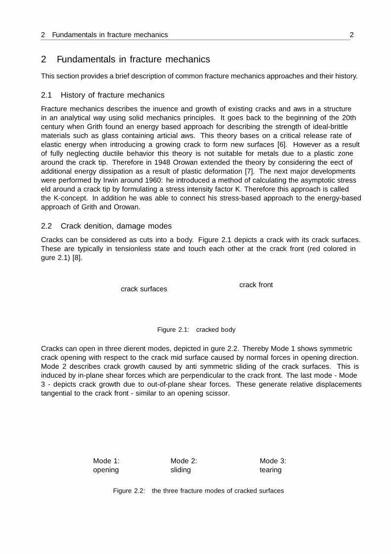
Cracks can be considered as cuts into a body. Figure 2.1 depicts a crack with its crack surfaces.These are typically in tensionless state and touch each other at the crack front (red colored infigure 2.1) [8].
crack surfaces crack front
Figure 2.1: cracked body
Cracks can open in three different modes, depicted in figure 2.2. Thereby Mode 1 shows symmetriccrack opening with respect to the crack mid surface caused by normal forces in opening direction.Mode 2 describes crack growth caused by anti symmetric sliding of the crack surfaces. This isinduced by in-plane shear forces which are perpendicular to the crack front. The last mode - Mode3 - depicts crack growth due to out-of-plane shear forces. These generate relative displacementstangential to the crack front - similar to an opening scissor.
Mode 2:sliding
Mode 3:tearing
Mode 1:opening
Figure 2.2: the three fracture modes of cracked surfaces

2 Fundamentals in fracture mechanics 3
2.3 Linear elastic fracture mechanics
Linear elastic fracture mechanics (LEFM) act on the assumption of small scale yielding which hasto be evaluated with special care for the corresponding material, structure and loading case. Formetals and brittle materials this assumption is fulfilled in most cases. More information can befound in literature and [9], [10].
2.3.1 Stress based approach
In the stress based LEFM approach, a crack will propagate, when a critical stress intensity factorKC , which is considered as a material property, is reached. Figure 2.3 shows a large panel witha transverse crack of the length of 2a subjected to uniform tensile stress σ0, which corresponds topure Mode 1 crack opening. In addition, the asymptotic stress field on the crack tip is depicted.This is derived from the stress field around the crack tip in polar coordinates. Since the stressesbecome infinite at the crack tip, a scaling factor for the stress field around the crack tip is induced,which in fact is the stress intensity factor K. Equation 2.1 shows the stress intensity factor for theexample above. More derivations for specific crack cases can be found in [8, p.82 ff.].
2a
x
y
z
σ0
σ0
x, r
σy
Figure 2.3: cracked infinite plate with asymptotic stress field at the crack tip
K1 = σ0√πa (2.1)
The critical value KC , where a crack starts to propagate, is dependent on the constraint. In planestress condition, higher values are achieved than in plane strain condition, where it converges toa minimum value after a certain specimen thickness. This plateau-value is called the plane strainfracture toughness KC and the value sought for. For characterization of the individual fracturetoughnesses of materials, standardized testing methods are provided by well-established institutesfor standardization [9, p.131], [8, p.103 f.].
2.3.2 Energy based approach
As mentioned in section 2.1 already, Griffith formulated a criterion for crack propagation based onan energy balance which was augmented by Orowan. In this concept, the infinitesimal decrease ofpotential energy Π of the specimen with respect to an increase in crack surface A, which is scaledby the crack length a in the two dimensional case, is considered. This term is called the energy

2 Fundamentals in fracture mechanics 4
release rate G, depicted in equation 2.2, which can be seen as material parameter similarly to KIC
in the stress-based concept. Thereby Π is the sum of outer (external energies) and inner potentialenergy (elastic strain energy), depicted in equation 2.3 [8, p.105].
G = −∂Π∂a
(2.2)
Π = Πa + Πi (2.3)
In the case of a linear elastic material, the K-concept can be inserted which leads to a quadraticconnection between K and G, depicted in equation 2.4. Thereby E′ corresponds to the Young’smodulus in plane stress state and E′ = E
1−ν2 in the case of plane strain condition. This assumptionis valid for pure Mode 1 as well as pure Mode 2 and pure Mode 3 loadings [8, p. 108].
G = K2I
E′(2.4)
Similar to the stress-based approach, standardized testing-methods are provided by well-establishedinstitutes for standardization. Comparing the deviations of these two approaches, one can implythat the stress-based one is a more local method where the energy-based concept represents a globaldefinition. For the reason of easier calculation at discretized models such as finite element models,the energy based approach is commonly preferred.
2.4 Mode mixture
In the general loading case more than one damage mode may occur simultaneously. Therefore thebehavior under mixed mode condition has to be covered by a rule since they influence each other.This is particularly interesting in adhesive or interface layers as a result of a pre-defined cracksurface.Many adhesive bonds or interfaces between laminated composites exhibit different fracture tough-nesses in the individual damage modes and nonlinear mixed mode behavior.
A simple criterion is the Power-Law fracture criterion which is depicted in equation 2.5. Theexponents n1, n2 and n3 are material constants which have to be obtained by mixed mode materialtests. When the fracture variable f reaches 1, the crack propagates. In addition, the exponents n1to n3 can be unified to one uniform exponent α = n1 = n2 = n3, which is done frequently. Figure 2.4shows some 2D fracture curves for the Power-law approach. Thereby for α = 1, the criterion reducesto the linear fracture criterion and for α = 2, an elliptical fracture curve is obtained.
f = GequivGC,equiv
=(G1G1C
)n1
+(G2G2C
)n2
+(G3G3C
)n3
(2.5)
2 Fundamentals in fracture mechanics 5
0 0.2 0.4 0.6 0.8 10
0.2
0.4
0.6
0.8
1
G1G1C
G2
G2C
α = n1 = n2 = 1α = n1 = n2 = 2n1 = 2, n2 = 1
Figure 2.4: example for the BK criterion
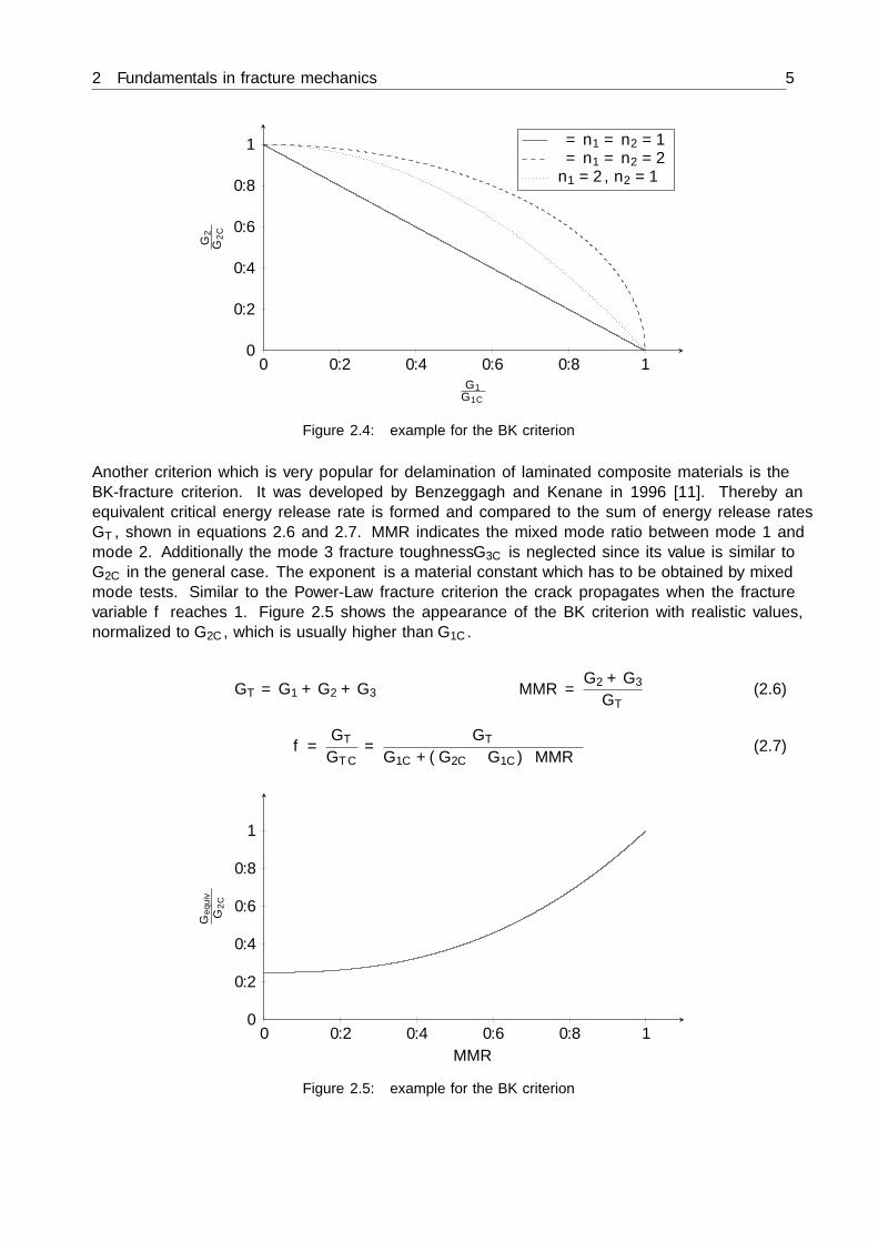
Another criterion which is very popular for delamination of laminated composite materials is theBK-fracture criterion. It was developed by Benzeggagh and Kenane in 1996 [11]. Thereby anequivalent critical energy release rate is formed and compared to the sum of energy release ratesGT , shown in equations 2.6 and 2.7. MMR indicates the mixed mode ratio between mode 1 andmode 2. Additionally the mode 3 fracture toughness G3C is neglected since its value is similar toG2C in the general case. The exponent η is a material constant which has to be obtained by mixedmode tests. Similar to the Power-Law fracture criterion the crack propagates when the fracturevariable f reaches 1. Figure 2.5 shows the appearance of the BK criterion with realistic values,normalized to G2C , which is usually higher than G1C .
GT = G1 +G2 +G3 MMR = G2 +G3GT
(2.6)
f = GTGTC
= GTG1C + (G2C −G1C) ·MMRη (2.7)
0 0.2 0.4 0.6 0.8 10
0.2
0.4
0.6
0.8
1
MMR
Geq
uiv
G2C
Figure 2.5: example for the BK criterion

3 Fundamentals of laminated composite materials 6
3 Fundamentals of laminated composite materialsAs the name implies, laminated composites consist of two or more different components which forma heterogeneous structure. In general, the aim of composites is to obtain a material with better char-acteristics than the individual components would have. Due to the different material properties andhigh aspect-ratio (length to diameter) of the components in case of laminated composites, namelyfibers and matrix, they show highly anisotropic material properties. The fibers are responsible forthe high strength and stiffness of the material while the matrix acts as power transfer between theindividual fibers [12]. In nature this combination can be found in many bionic structures such aswood or bones due to the superior strength- and stiffness-to-weight ratio which satisfies the maintarget of bionic design: efficient material usage.
3.1 Material-composition and macroscopic structure
In the following section different materials and possible configurations of the individual componentsare depicted.
3.1.1 Fiber-materials
Materials show highly increased material properties in fiber form than compared to the correspond-ing bulk material, as depicted in figure 3.1. This is due to the sharp reduction of inner defects inthe fiber form. In many cases, another major contribution to these significantly higher propertiesis the fact of molecular orientation. A good example are polymer fibers, which have randomly en-tangled polymer chains aligned in fiber direction when produced in a spinning process and/or whenstretched, as shown in figure 3.2. This effect also leads to an increase in stiffness in fiber direction.
tensile strength / MPa
fiber thickness / µm20100
3000
2000
1000
extrapolates to 11GPa
extrapolates to approximatestrength of bulk glass (170MPa)
Figure 3.1: diameter-strength relationship by the example of glass [13]
3 Fundamentals of laminated composite materials 7
Figure 3.2: left: fiber pierced out of a polymer block; right: spinned fiber
The most important properties of fibers are high specific mechanical properties and compatibilityof its surface with the corresponding matrix. This is why e.g. Polyethylene fibers are not used incomposite laminates due to their highly inactive surface in untreated condition besides their ratherhigh specific properties at low cost.In the following the most common fibers are reviewed in a short manner.
Carbon fibers
Carbon fibers consist of graphene layers in turbostraticconfiguration, which are mainly oriented in fiberdirec-tion as depicted in figure 3.3. The fact that graphenecontains delocalized electrons leads to electrical con-ductivity, which can lead to corrosion when in con-tact with metals and shielding of radio waves. Twomajor precursors are available for producing carbonfibers, Polyacrylnitrile-fibers (PAN) on one hand andpitch-fibers on the other. Pitch fibers are less expens-ive in production but show significantly lower tensilestrength. The properties of carbon fibers can be variedin a broad range by thermal treatment which influ-ences carbon content and orientation of the strongestcarbon links along fiber direction [12, p.31]. Carbonfibers show high-end properties at a rather high price.
Figure 3.3: turbostatic molecular struc-ture of carbon fibers [13]
Glass fibers
Glass fibers are drawn from specific glass melts - a blend of sand, limestone and other oxidiccompounds [12]. Their molecular structure is still amorphous and they show the glass-specificproperties such as inertness, high corrosion resistance and hardness. Several types of glassfibersare existing with different strength but similar stiffness. The most common type thereby is E-glasswhich shows good mechanical properties at favourable price.

3 Fundamentals of laminated composite materials 8
Aramid (DuPont Kevlar®) fibers
These fibers are based on spinned and stretched Aramid which is a liquid crystalline polymercontaining a stiff molecular structure as a result of many aromatic rings. Kevlar fibers show highspecific tensile strength and toughness but absorb moisture and degrade at UV-exposure.
Comparison of the most common fibers
Figure 3.4 shows stress-strain curves of high modulus- (HM-), high strength- (HS-) carbon, E- andS-glass, boron and Kevlar fibers. It can be seen that the increased modulus of the HM-carbonfiber leads to major drawbacks in strength versus the HS-carbon fibers. S-glass leads to overallbetter performance compared to E-glass but at much higher price due to low production volumes.Taking the density into account Kevlar fibers which seem to be unobtrusive in this chart becomevery competitive to carbon-fibers. Summarized the design engineer has to keep the fiber types’mechanical and economical advantages and drawbacks in mind for proper material selection at therespective case of application.
2
4
21 3 4ε / %
tensile strength / GPa
Car
bon
HM Bor
on
Car
bon
HS
Kevlar 49 S (R)-glass
E-glass
Figure 3.4: comparison of selected fiber types [13]
3.1.2 Fiber configurations
The fibers can be embedded in the matrix in many different ways. This work is focused on unidirec-tional (UD) and woven continuous fiber fabrics as shown in figure 3.5. Thereby bunches of theseindividual fibers which have a thickness of only a few microns are aligned to rovings or twisted toyarns. In woven fabrics these fiber-bundles are woven to fabrics similar to cloth. One individuallayer of fibers is called a ply. These are stacked further together layer-by-layer over each other toa laminate. Thus, using different ply orientations with respect to the global laminate coordinatesystem, the laminate can be tailored to the specific load case. Using UD fabrics, fiber contents of70% can be reached in the laminate. Due to the warpage of fibers in woven fabrics, fiber contentsare limited to about 60% [14].
3 Fundamentals of laminated composite materials 9
Figure 3.5: left: UD fabric; right: woven fabric [14]
3.1.3 Matrix-materials
The main purpose of the matrix material is to form a strong bond with the fiber surface to holdthem together and transfer the loads to the fibers. It also has to carry transversal and interlam-inar stresses. For manufacture, the matrix material has to be low-viscous with good wettability.In general there are many different options for matrix materials such as thermoplastic polymers,thermosets and other specialities. The most common matrix material for laminated composites areepoxy resins due to their favourable properties in processing and good mechanical performance.However as with other thermosets, recyclability is still a major drawback hence they cannot bebrought back to some sort of deformable state again without destroying them.
3.2 Damage mechanisms
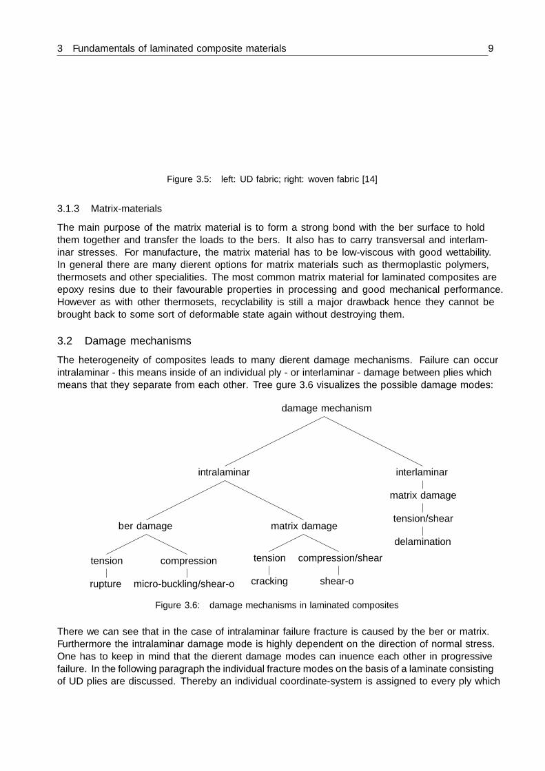
The heterogeneity of composites leads to many different damage mechanisms. Failure can occurintralaminar - this means inside of an individual ply - or interlaminar - damage between plies whichmeans that they separate from each other. Tree figure 3.6 visualizes the possible damage modes:
damage mechanism
intralaminar
fiber damage
tension
rupture
compression
micro-buckling/shear-off
matrix damage
tension
cracking
compression/shear
shear-off
interlaminar
matrix damage
tension/shear
delamination
Figure 3.6: damage mechanisms in laminated composites
There we can see that in the case of intralaminar failure fracture is caused by the fiber or matrix.Furthermore the intralaminar damage mode is highly dependent on the direction of normal stress.One has to keep in mind that the different damage modes can influence each other in progressivefailure. In the following paragraph the individual fracture modes on the basis of a laminate consistingof UD plies are discussed. Thereby an individual coordinate-system is assigned to every ply which

3 Fundamentals of laminated composite materials 10
is aligned along the fiber direction (1), perpendicular to the fibers (2) and the thickness direction(3), as shown in figure 3.7.
Figure 3.7: ply coordinate system [2]
As depicted, there are different nomenclatures available for the individual directions. In this workthe number-based one is used due to the fact that it is commonly used in anglo-saxon countries.
3.2.1 Intralaminar damage
Intralaminar failure can occur in the fiber, matrix or in the interface between them. In contrast tometals, tension and compression loads must be treated differently. This is due to the nature of afiber, which cannot carry compressive loads on its own, similar to a rope or a cable.
Fiber failure
In the static tension loading case, fiber failure mainly occurs when the ply is loaded in 1-direction.For the reason of a statistical fiber strength distribution, which commonly follows a Weibull-shape[12, p.28], damage occurs gradually. This means that fracture starts at the weakest individualfibers which causes stiffness-degradation. Furthermore at higher loads this leads to failure of wholefiber-bundles. Therefore fiber-failure is not fully brittle but quasi-ductile [2, p.346].
When applying compressive loading in 1-direction, failure is triggered by the loss of stability similarto the buckling of rods but on a micro-mechanical level. In contrast to rods where buckling occursin bending mode in FRP materials, it takes place in shear mode due to the low shear-stiffness ofthe material. This mechanism is called micro-buckling, which is depicted in figure 3.8.
Figure 3.8: micro-shear-buckling of fibers under compression load in 1-direction [2, p.351]
3 Fundamentals of laminated composite materials 11
This form of failure can occur in in-plane direction but also in out-of-plane direction at certainlayups. Due to the high dependency of the compressive strength on the fiber-angle, the fibers haveto be aligned in loading-direction as perfect as possible without any waviness to assure maximumstrength values. To avoid this failure mode high accuracy as well as exact and careful handlingduring the whole production process is demanded.In-plane shear-stress also reduces the compressive strength in 1-direction, R−11. But one has tokeep in mind that most composite structures are thin-walled and therefore global loss of stabilitygenerally occurs before the described micro-buckling. Critical areas for micro-buckling are edgesof holes where the fibers buckle into the hole due to stress increase near the hole or boundariesat bending-beams which are bended by transversal loads due to the shear-stresses and the lack ofsupport on the edges [2, p.362].
Matrix failure
Matrix failure or in-plane inter-fiber-failure (iFF) is a more complex phenomenon. Generally onehas to separate between the action plane which is the plane of maximum load in the material andthe fracture plane. These planes may not fall together in some cases as A. Puck discovered in 1992in UD layers [2].
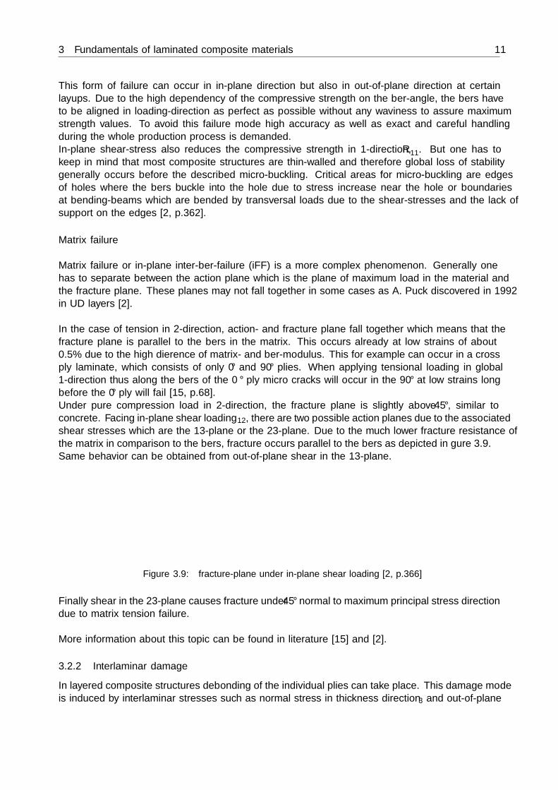
In the case of tension in 2-direction, action- and fracture plane fall together which means that thefracture plane is parallel to the fibers in the matrix. This occurs already at low strains of about0.5% due to the high difference of matrix- and fiber-modulus. This for example can occur in a crossply laminate, which consists of only 0° and 90° plies. When applying tensional loading in global1-direction thus along the fibers of the 0° ply micro cracks will occur in the 90° at low strains longbefore the 0° ply will fail [15, p.68].Under pure compression load in 2-direction, the fracture plane is slightly above 45°, similar toconcrete. Facing in-plane shear loading τ12, there are two possible action planes due to the associatedshear stresses which are the 13-plane or the 23-plane. Due to the much lower fracture resistance ofthe matrix in comparison to the fibers, fracture occurs parallel to the fibers as depicted in figure 3.9.Same behavior can be obtained from out-of-plane shear in the 13-plane.
Figure 3.9: fracture-plane under in-plane shear loading [2, p.366]
Finally shear in the 23-plane causes fracture under 45° normal to maximum principal stress directiondue to matrix tension failure.
More information about this topic can be found in literature [15] and [2].
3.2.2 Interlaminar damage
In layered composite structures debonding of the individual plies can take place. This damage modeis induced by interlaminar stresses such as normal stress in thickness direction σ3 and out-of-plane

3 Fundamentals of laminated composite materials 12
shear stresses τ13 and τ23. It is similar to intra-laminar matrix fracture but with planar propagationresulting due to the absence of crack arresters such as fibers. As a consequence they can impactthe laminate properties significantly due to high spreading. In many cases delamination is causedby iFF-damage (from an impact for example) or resulting from manufacturing imperfections suchas voids. Drilling also produce delaminations between the top- and the bottom layers as a result ofpeel-up and push-out mechanisms as it is shown in figure 3.10 [16].
Figure 3.10: left: peel-up delamination; right: push-out delamination [16]
Another causes of delamination can be ply-dropoffs, free edges or curved sections which induceinterlaminar stresses. In the case of free edges at the example of a cross-ply (consists of 0°- and90°-plies) under tension in laminate 1-direction, contraction of the 90°-layers is restrained due to thestiff fibers. This leads to peel-stresses at the outer edges of the 0°-layers as we can see in figure 3.11.In curved sections tension stresses in radial direction appear when the specimen is bended contraryto the curvature, which lead to delamination([2, 17]), depicted in figure 3.12.
Figure 3.11: interlaminar stresses caused by restrained transverse contraction [2, p.388]
F F
σr
Figure 3.12: interlaminar radial stresses in bended curved beams
Considering an existing interlaminar pre-crack in a laminate, all of these phenomena can be dividedinto three damage modes, as mentioned in section 2.2. These are the opening mode 1, the in-plane

3 Fundamentals of laminated composite materials 13
shear mode 2 and the out-of-plane shear mode 3.Contrary to metals where crack growth occurs primarily perpendicular to the maximum principalstress direction (mode 1), in composite materials a damage propagates along the interface layerdue to the heterogeneous, layered structure. Therefore in realistic load cases mode mixing of theindividual crack modes occurs which leads to the question of a proper mathematical description infracture mechanic approaches. Further details are described in section 3.3.2.
3.3 General 3D modeling approach in Finite Element Analysis
For modeling laminated composites, several possibilities are available. One can model the wholelaminate, ply-stacks or individual plies with or without interfaces in between. Higher modelingaccuracy results in more precise representation of the real structure but significantly increasescalculation time. Therefore one has to find a compromise between good representation of thestructure and needed simplifications which leads to proper modeling strategy selection for the presentproblem. The work focuses on three-dimensional (3D) modeling techniques for the reason of theapplicability of techniques for interface damage modeling. Therefore, solid and continuum shellelements will be used.
3.3.1 Element types for laminate modeling
In this section, suitable element types for 3D-modeling of laminated composites are reviewed. Ingeneral, elements can use linear shape functions resulting in one node at each corner or they canuse quadratic shape functions which results in an additional node at all edges. Thereby formerelements give a linear displacement distribution over the edge and latter elements give quadraticdisplacement distributions over the edge which improves their accuracy substantially.Stresses are calculated in integration points. In addition there is an option of reduced integrationresulting in a decrease in calculation time but generating the problem of hour-glassing at first-order elements in some cases. Additional information can be found in literature and FEM-packagemanuals [18].
Shell elements
When modeling with shell elements, a thin-walled structure is reduced to a two-dimensional refer-ence surface - the mid surface in the common case. Figure 3.13 shows a structural body and thecorresponding discretization to a shell with linear quadrilateral elements. Additionally triangularelements are available for complex shapes. However these need higher mesh refinement for the samelevel of accuracy. This results from the natural shearlocking in triangular structure statically de-termined shape (which is used in frameworks for example) and that leads to an undesired increasein element stiffness.

3 Fundamentals of laminated composite materials 14
structural body shell discretization
Figure 3.13: shell discretization of a structural body
The thickness of a shell element is defined through the section property definition, thereby thepositive thickness direction has to be determined. In general shell elements have displacementand rotational degrees of freedom. For calculating the plate behavior, these kind of elements have aselectable number of section points over the thickness. In addition, some of them include deformationinduced by transverse shear stresses, which is important at laminated composite structures forexample or can be used for large deformations. In fact shell elements lead to efficient calculationdue to a high level of simplification. However, using them for discretizing more complex structuralparts can lead to high errors between simulation and reality as a result of oversimplification. Thisis caused by reducing the problem to plane stress or plane strain condition in thickness direction.
Solid elements
For full three dimensional discretization of complex structural bodies solid elements are available.Because they are defined in all three coordinate directions, three dimensional stress states canbe calculated properly. However analyses with solid elements are much more time consuming,especially with quadratic formulation, since significantly more elements are needed for discretization.Furthermore in the case of bending problems more than one element should be used over thethickness for proper stress calculation. For more complex shapes tetrahedral elements are available.However as well as in the two dimensional case these need higher mesh refinement as a result ofthese elements’ natural stiffening. Figure 3.14 shows a structural body and the corresponding soliddiscretization with linear hexaedral elements.
structural body solid discretization
Figure 3.14: solid discretization of a structural body
Continuum shell elements
Continuum shell elements, which are available in Abaqus for example, base on a three-dimensionalbody. These elements have displacement degrees of freedom only. They look like three-dimensional

3 Fundamentals of laminated composite materials 15
solid elements but behave similar to conventional shell elements which leads to reduced calculationtime compared to solid elements. In addition the bending behavior is included analogous to shellelements so only one element over the thickness is needed. Shear deformation is covered by firstorder shear deformation theory (FSDT), which makes them suitable for laminated composites sincethey exhibit low shear stiffness through the thickness. Furthermore they include thickness change.Other than shell elements, they can be stacked to provide a more refined through-thickness response[18].
3.3.2 Techniques for interface damage modeling
For including interlaminar damage behavior when modeling laminated composite structures, theinterfaces between the layers have to be modeled separately. Therefore the two most commontechniques for modeling interface damage in finite element models are presented in the following.
Virtual Crack Closure Technique
The virtual crack closure technique (VCCT) is based on linear elastic fracture mechanics (LEFM,see section 2.3) and can be used for the simulation of delamination phenomena in layered structuressuch as laminated composite materials. Figure 3.15 depicts a 2D finite element model using linearquad elements with two partially connected layers, an upper layer u and a lower layer l. Additionallythere is a cracktip at the overlapping of the connected nodes n of each layer.
z
x
∆wm
∆umml
mulu
ll
n o p
Xun
X ln
Zun
Z ln
a ∆a ∆a ∆a
Figure 3.15: VCCT for four-noded 2D elements
In general the assumption of crack closure techniques is that the energy ∆E released when openinga crack by the length of ∆a is equal to the energy for closing the same crack. Therefore the actingforces Zn and Xn (Zun = Z ln equilibrium, same with Xn) on each layer’s node n are calculated witha finite element analysis. It is obvious that Zn induces delamination in mode 1 and Xn in mode 2.In general a second calculation is needed where the bonding of the nodes n is released in order tocalculate the opening displacement of the crack tip.This is done in the crack closure method [19, p.3]. However, in the virtual crack closure technique(or modified crack closure method), it is assumed that a crack extension of ∆a from a + ∆a toa + 2∆a (from node n to node o) does not significantly alter the state at the crack tip. Thereforethe displacements at separation of the nodes n is assumed to be equal to the displacements of nodes

3 Fundamentals of laminated composite materials 16
mu and ml. This leads to the following equation for the work required to close the crack for thetwo-dimensional case:
∆E = 12 · [Xn ·∆um + Zn ·∆wm] (3.1)
For calculating the energy release rates G = ∆E∆A , different formulas are obtained for different element
types [19]. In the case of linear 2D quad elements which are used above in figure 3.15, G1 and G2are calculated as shown in equations 3.2. For other element types the author refers to the literature,in particular [19].
G1 = − 12∆a · Zn ·∆wm G2 = − 1
2∆a ·Xn ·∆um (3.2)
The calculated energy release rates are compared to the corresponding fracture toughnesses to verifyany crack onset or crack propagation, see sections 2.4 and 4.4. If the criterion is fulfilled, the nodeis released and the procedure repeats for the next crack tip node. Alternatively, an appropriatenumber of cycles until the crack has propagated to the next node of a finite element mesh can becalculated.
Cohesive Zone Modeling
Cohesive zone models (CZM) base on independent works of Dugdale [20] and Barenblatt [21], whoaugmented linear elastic fracture mechanics by nonsingular solutions for the opening displacementand traction fields of the crack faces at the crack tip. Therefore Dugdale used elastic perfectly plasticmaterial behavior, which generates a plastic zone in front of the crack tip, that virtually elongatesthe crack tip by a certain distance d, dependent on a critical crack tip opening displacement δC[8, p.164]. Barenblatt looked for specific shapes of the crack tip, in which the singularity vanishes,hence the stresses on the crack tip become finite. Despite the different initial approaches, the samesolution is obtained.
Figure 3.16 shows a cohesive zone model applied on a mode 1 crack and figure 3.17 a simple, bilinearcohesive law with linear stiffness degradation after a certain σ0, which corresponds to the damageof the cohesive zone. There, the elastic region in former figure corresponds to the linear rising slopeat the beginning in latter, until δ0 is reached. After exceeding δ0, the cohesive zone is damagedand the stiffness degrades linearly, which is described by K(D). Thereby the red line in figure 3.17indicates the loading and unloading path of a damaged area cohesive zone. When δC is reached,the damage reaches 1 and the cohesive stiffness drops to 0, which means that the bond separates.Comparison of this theory to elastic plastic fracture mechanics (EPFM) shows that the area underthe traction law represents the critical strain energy release rate GC (see [8, 168 ff.]). When δC isequal to δ0, which corresponds to ideal elastic material followed by a instant stiffness drop to 0, theinelastic damage process zone in figure 3.16 vanishes and hence, an ideal brittle material responseas in energy based LEFM (see section 2.3.2) is obtained.

3 Fundamentals of laminated composite materials 17
δC
da
x
z
σ(x)
true crackD=1
damage process zone0<D<1
elastic regionD=0
Figure 3.16: cohesive zone at a mode 1 crack
D=0
D>0
D=1
σσ0
δ0
δ
δC
traction separated
1
K0 1K(D) = (1−D)K0
GC
Figure 3.17: bilinear equivalent one dimensional cohesive traction law
Many other different traction laws were created to represent specific material behavior, such asthe exponential law depicted in figure 3.18. In general, the point of onset of damage as well asthe unloading behavior of the damaged material can be set individually. The red line depicts asuggestion for the loading and unloading behavior in damaged state at the exponential traction law.However, the unloading behavior can differ from the loading behavior, which induces hystereses.

3 Fundamentals of laminated composite materials 18
σσ0
δ0
δ
δC
traction separated
D=0
D>0
GC
Figure 3.18: exponential one dimensional cohesive traction law
Mixed mode is treated by interpolating between traction laws of the same type for mode 1 andmode 2/3, as it can be seen in figure 3.19, where simple quadratic interpolation is used:
σ
δ1
δ2 δm
δ1C
δ2C
δmC
Figure 3.19: mixed mode treatment for cohesive zones [22, p. 2-805]
As a conclusion, cracks are not modeled as discontinuities due to the reason that the model isbased on continuum damage mechanics. Therefore, other than in VCCT, no initial crack is needed.This means that the undamaged interface and the crack initiation can be modeled. However, anappropriate cohesive traction law with stiffness and (un-) loading behavior under damaged conditionhas to be determined. Thus, for simple bilinear traction laws, Turon et al. created guidelines forobtaining proper parameters for numerical FEM simulations in [23].

4 Fundamentals in fatigue 19
4 Fundamentals in fatigue
4.1 Fatigue: History and general definition
In the 19th century when railways came up, unexpected failure of wagon axles after a certain timeof use lead to first fatigue experiments by August Wöhler. This lead to the famous S-N or "Wöhler-"curves, where the applied loading was described over the number of cycles to failure for metals. Ingeneral, fatigue means the impairment, crack initiation and propagation under repeated loading.Thereby the load level is lower then in the static case. The loading can be periodic, aperiodic,deterministic or even stochastic. In high cycle fatigue (Number of cycles to failure over 1 · 104),rupture commonly occurs without high plastic deformation even at ductile materials. Figure 4.1shows an example catastrophic failure of a turbine shaft due to high cycle fatigue loading, wherecrack propagation occurred from the inside. Therefore fatigue is a critical failure mode in cyclicloaded structural parts.Additional information can be found in literature and [24–26].
Figure 4.1: turbine shaft of a 300MW steam turbine set [27]
4.2 Design philosophies
When designing a structure, the engineer has to choose between two fundamental design philosophies[28]:
� safe-life concept: This concept acts on the restriction of no damage in the whole lifetime ina structural part. Therefore, high safety factors and over-dimensioning is needed in general.
� fail-safe concept: In the fail-safe or damage-tolerant concept, the structural component isdesigned as a redundant system, in which flaws in a structure do not induce failure of thewhole component to a certain extent over the lifetime. This means, that cracks are allowedto a certain size.
The fail-safe concept is of special interest in composite structures, since other than in metals, thestage of damage initiation is rather short compared to the stage of propagation (see section 4.6).This results in excessive over-dimensioning when a safe-life concept is used in the dimensioning ofcomposite structures.

4 Fundamentals in fatigue 20
4.3 Loading conditions
For the characterization of a certain periodic loading, significant variables are introduced. In fig-ure 4.2, a sinusoidal loading σ(t) with the cycle duration T and specific levels of maximum andminimum stress σmax and σmin is shown. From these, further parameters, namely the mean andamplitude stress σm and σa can be derived, as depicted in equations 4.1:
0 T 2T
σmin
σm
σmax
time t
cyclic
stressσ(t)
Figure 4.2: example for a periodic sinusoidal loading
σm = σmin + σmax2 σa = σmax − σmin
2 (4.1)
Furthermore another representative variable for describing the loading condition - the stress ratioR - can be calculated as shown in equation 4.2:
R = σminσmax
(4.2)
Thereby specific values are obtained for different loading conditions:
� between 0 < R < 1, the specimen is subjected to tension-tension loading
� between 1 < R < ∞, the specimen is subjected to compression-compression loading
� between -∞ < R < 0, the specimen is subjected to tension-compression loading
� at R=0, the specimen is subjected to pulsating tension loading
� at R=±∞, the specimen is subjected to pulsating compression loading
These five variables are dependent on each other, leaving two degrees of freedom and represent acertain fatigue loading condition. Classifications of more general loadings, which usually occur inreal applications, are primarily based on these (see section 4.5.1).

4 Fundamentals in fatigue 21
4.4 Fatigue damage evolution
In metals, fatigue crack growth starts with microscopic cracks, which emerge for example fromdislocations. Multiple microscopic cracks form a macroscopic, sharp crack of a length of about1mm. This procedure is called damage or crack initiation.Dependent on the level of the applied cyclic loading, an existing macroscopic crack is faced toa certain rate of crack growth then, when a certain threshold level is reached. Under moderateloadings, it grows to a critical length until the crack growth becomes unstable and final ruptureoccurs. Figure 4.3 shows these individual stages of fatigue damage evolution at the example of asimple metal component, which is subjected to a cyclic fatigue loading F (t):
crackinitiation
propag
ation
finalrupture unstable
propagation
stablepropagation
F(t)
F(t) F(t)
F(t)
F(t)
F(t)
Figure 4.3: stages of fatigue damage evolution
As depicted, in metals, one or only a few dominant macroscopic cracks control the fatigue life ofa structural component in general. Therefore, e.g. in aeronautical structures, emerging cracks aremonitored to estimate the remaining fatigue life. However, this is not the case in every material, asit will be shown for laminated composites in section 4.6.
4.4.1 Damage initiation
In general, damage initiation, also called damage nucleation, is treated by S/N-curves, in which themaximum allowed stress amplitude over the number of cycles is depicted for specific levels of themean stress. For statistical reasons, the curve has to be considered as a band with high probabilityof failure on the upper border and low probability of failure on the lower boarder, which follows alogarithmic normal distribution in general case. Therefore, every S/N-curve has a certain survivalprobability, which is 95% in most cases [24, p.44 ff.]. Regarding the shape of the S/N-curve, twodifferent behaviors can be observed:
� Type 1 behavior, in which after a certain number of cycles, which is 1 · 106 to 1 · 107 cyclesin normal case, the maximum allowed stress amplitude reaches a plateau, which is the fatigueendurance limit. This occurs in low-alloy steels and titanium for example.

4 Fundamentals in fatigue 22
� Type 2 behavior, in which the degradation is also reduced after a certain number of cycles,but does not reach a plateau. However, to define an endurance limit with high reliability, aultimate cycle number of 2 · 106 to 1 · 109 cycles is commonly taken [24, p.20].
Figure 4.4 shows these two types of S/N-curves with the regions of low cycle fatigue (LCF) to about1 · 104 and high cycle fatigue (HCF) from there on:
Ne Nelog(N)
log(σA)
log(N)
log(σA)
σE σELCF HCF LCF HCF
Figure 4.4: types of S/N-curves: Type 1 (left), Type 2 (right) [25, p.361]
For low cycle fatigue applications of ductile metals, which is up to about 5 · 105 cycles, ε/N-curvesare frequently used since they better represent the occuring elasto-plastic deformations [24, p.33ff.].For the numerical description of S/N-curves, many researchers such as Basquin, Stromeyer, Palmgren,Bastenaire or Stüssi, proposed suitable models. Equation 4.3 shows Basquin’s law, which representsthe polynomial decrease of the maximum stress amplitude over the cycle number in the region offinite life fatigue strength at a given mean stress. Thereby σe indicates the fatigue strength of theamplitude whereas Ne expresses the endurance limit and k controls the slope of the curve.
σa = σe ·(Ne
N
) 1k
(4.3)
Multiple S/N-curves with different mean stresses can be assembled together to constant life diagrams(CLD), for example according to Smith or Haigh, then. Figure 4.5 shows a qualitative example ofa constant life diagram according to Haigh with a linear curve according to Goodman and equalbehavior on positive and negative mean stress:
(R=1) −σy 0 σy (R=1)
σe
σy
(R=-1)
mean stress σm
stress amplitude σa
N=1N=104
N=105
N=Ne=107
Figure 4.5: linear constant life diagram according to Haigh

4 Fundamentals in fatigue 23
Thereby the line for N=1 indicates the static strength σy whereas Ne shows the endurance limitwith σa = σe at σm = 0 (R=-1). Other curve shapes are proposed by Soderberg, Gerber or Morrowfor example. More information can be found in literature and [24–26].
4.4.2 Onset of propagation
For the onset of propagation of an existing flaw, Murri, Salpekar and O’Brien proposed a methodfor determining the timespan for the formation of a macroscopic, sharp crack for mode 1 crackgrowth [29]. Similar to a S/N-curve, dependent on the number of cycles, a certain maximum strainenergy release rate is needed for crack onset, as shown in equation 4.4:
G1,max = c ·Nd (4.4)Thereby the constants c and d are material constants. A standardized testing method for themeasurement of the onset of propagation in mode 1 is presented in ASTM D 6115 - 97. As statedin [30], the initial condition of the crack tip is essential for the onset of damage. This means,that the onset differs significantly, if e.g. a specimen is pre-cracked or not. A similar crack onsetdetection criterion is implemented in the Abaqus low cycle fatigue criterion, which is described insection 6.2.1.
4.4.3 Damage propagation
After the formation of a sharp, macroscopic crack while being subjected to a sub-critical fatigueloading, crack propagation occurs. Figure 4.6 depicts the rate of crack growth over the effectivestress intensity factor ∆K = Kmax − Kmin on a double logarithmic plot. It can be seen that thecurve can be partitioned into three significant regions:
� region I, in which crack growth slowly starts at ∆Kth = Kth − Kmin, with a rising rate ofcrack growth with increasing ∆K
� region II, where stable crack growth occurs
� region III, where accelerated crack growth occurs until reaching the relative static criticalstrain energy release rate ∆KC = KC −Kmin
∆KC∆Kth log(∆K)
I II III
log(dadN
)
Figure 4.6: qualitative crack growth curve of a macroscopic crack [25, p.356]

4 Fundamentals in fatigue 24
For region II, Paris and Erdogan [31] found a power law relationship, in which the crack growthrate is dependent on the relative stress intensity factor ∆K = Kmax −Kmin in a cycle, depicted inequation 4.5. There, C and m are material constants.
da
dN= C · (∆K)m (4.5)
Since the so-called Paris law is only valid for a given stress ratio R, the model was expandedby several researches to cover the effect of the stress ratio, for example by Walker for aluminumalloys [32]. In addition, many other proposals and modifications are given by researchers to coveradditional effects such as the non-polynomic regions near the threshold and critical value, loadfrequency, temperature and so on, which can be found in literature.
4.5 Treatment of general load spectra
In most real applications, a structural element is subjected to variable amplitude loadings, whichcan be periodic, aperiodic or even random. In addition, the mean loadings can be variable as well.Therefore, a load-time function has to be classified to load spectra of constant mean and amplitudeloading and their individual contributions to the damage have to be considered to accurately estim-ate the fatigue life. In the following, common techniques for classification and damage accumulationare discussed.
4.5.1 Classification of general load spectra
For the classification of general load time functions, many methods were developed. One-parameterclassification methods focus onto the classification into certain load regions with respect to a certainattribute such as the peak value or when the function passes a load region. However, since stressratio effects are not covered by these methods, two-parameter classification methods were created.Other than in one-parameter methods, mean and amplitude loadings can be transformed back fromthe classification results. The most popular of them is the Rainflow-counting method for the reasonof a physical background in closed stress-strain hysteresis loops. With it, a transition matrix isobtained, which can be formed into a more demonstrative amplitude-mean value matrix, containingthe relative occurrences. With the help of a Haigh diagram and the Miner’s rule for linear damageaccumulation (see section 4.5.2), the individual fractions of damage can be calculated and addedtogether. When subjected to subsequent stress patterns, these matrices can be added together.Several researchers proposed modifications to overcome drawbacks such as sequence effects or openhysteresis loops. Additional information can be found in literature, in particular [24].
4.5.2 Damage accumulation
To obtain the total damage to a given number of cycles, the individual damages of the load spectrahave to be estimated and added together. The most popular damage accumulation rule is thePalmgren-Miner rule, where the incremental damage, ∆D, is estimated by comparing the numberof loading cycles, N , to the number of cycles to failure according to the corresponding S/N-curve,Nf , as done in equation 4.6:
∆D = ∆NNf
(4.6)
Fracture occurs, when∑
∆D = 1. As it can be seen, the Palmgren-Miner rule is linear. However, itdoes not account for sequence effects and interactions between the damage and the fatigue strengthobtained from the S/N-curve. Therefore, many researchers provided proposals for nonlinear damageaccumulation rules, which however need additional parameters to be identified [24, p.293 ff.].

4 Fundamentals in fatigue 25
4.6 Comparison of fatigue behavior of metals and laminated composites
In metals, the crack initiation phase is usually the dominant timespan in fatigue. After crackinitiation, one or only a few cracks dominate the crack propagation phase. These macroscopiccracks commonly propagate normal to principal stress direction at the crack tip, which is mode 1crack propagation (compare section 2.2). In laminated composites, many microscopic cracks emergefrom voids and weak fiber-matrix bonds in the matrix already at low cycle numbers, stopped byneighboring fibers. This leads to local stiffness degradation, which causes redistribution of loadpaths and further stiffness degradation in other regions. When the matrix is saturated with acertain amount of microscopic cracks, macroscopic cracks accumulate, which cause final failure ofthe structural part [25]. Since the formation of these macroscopic cracks occurs over a wide rangeof the fatigue life, crack propagation is the dominant mechanism in laminated composites. Inaddition, interlaminar matrix damage - namely delamination (compare section 3.2.2) - can emergefrom intralaminar matrix cracks. These propagate at rather high speed, since in between the layers,there are usually no crack arresters such as fibers. Furthermore delamination and intra-laminarfiber-matrix debonding decrease the supporting effect of the fibers in compression loading, whichcauses micro-buckling. Thus, interlaminar damage is of particular interest in fatigue.

5 State-of-the-art fatigue damage modeling techniques of laminated composites 26
5 State-of-the-art fatigue damage modeling techniques of lamin-ated composites
To overcome the peculiar, different fatigue behavior of laminated composite materials, many ap-proaches were already created. Since these overlap in many cases, differentiation into certain classesis a difficult task. Therefore, a rather general classification is presented in the following.
5.1 Laminate and lamina fatigue life estimation
The first and oldest class of composite fatigue models are leaned on the same treatment which isusually taken in metal fatigue. There, S/N-curves and constant life diagrams (CLD) are measuredfor a certain laminate with a defined ply stacking sequence (PSS). Since laminated composites showhighly nonlinear dependency of the stress ratio, as depicted in figure 5.1, piecewise linear CLD usingS/N-curves for several stress ratios lead to a better representation. For a continuous estimation overthe whole stress ratio spectrum for the reduction of experimental tests, some researchers tried todescribe the effect of stress ratio by fitting functions for the Haigh diagram. However, they are notconsistent over several material combinations and therefore, piecewise linear CLD with sufficientamount of stress ratio data is the most accurate choice in general [26, p. 127f]. Since these CLDsare only valid for a certain laminate with a specific PSS and material combination, a huge amountof material testing is needed.
Figure 5.1: piecewise CLD with interpolated lines for a [90/0/±45/0]S E-glass/polyester laminate [33, p.16]
Other approaches for estimating fatigue life are based on residual values of the laminate strengthor stiffness, as depicted in figure 5.2:

5 State-of-the-art fatigue damage modeling techniques of laminated composites 27
Figure 5.2: schematic degradation of strength and stiffness during constant amplitude fatigue loading [33,p.10]
In the case of residual strength models, the specimen has to break for derivation of the residualstrength, which induces a high amount of destructive testing needed, similar to CLDs. This resultsfrom the need of loading the specimens to certain number of cycles, followed by testing the remainingfatigue strength for every single point of the curve. Furthermore, residual strength remains ratherconstant until the end of fatigue life in laminated composite materials, where it suddenly decaysrapidly (sudden-death phenomenon). Residual stiffness usually changes significantly in earlier stagesof fatigue life and can be measured by non-destructive testing as it can be seen in figure 5.2. Thecurve can be divided into three regions: significant initial stiffness drop in early fatigue life, followedby little decrease over a wide range, until it drops significantly again in the region of final frac-ture. Furthermore, stiffness measurements show less scatter than strength based data. In fatiguetests with several specimen, for certain residual stiffnesses, probabilities of failure can be alloc-ated. In [34], these residual stiffness curves were used to derivate S/N-curves. These "Sc/N-curves"significantly reduce testing effort which collaborating well with conventionally measured S/N-curves.
Since multi-axial stress states are not covered by classical S/N approaches and the derivation ofequivalent stresses according to e.g. Mises or Tresca is not permissible for anisotropic materials,many researchers proposed multi-axial fatigue failure criteria. There, many of them, e.g. Hashin-Rotem [35], are based on S/N curves. However, most of them are limited to specific laminate typessuch as UD, cross-ply or angle-ply.Other approaches are extensions of static intralaminar failure criteria such as Tsai-Wu [36] or baseon strain energy density (e.g. Plumtree and Cheng [37]). Summaries of the wide spectrum of fatiguelife failure criteria can be found in literature, in particular [38, 39].

5 State-of-the-art fatigue damage modeling techniques of laminated composites 28
5.2 Progressive damage models
Since stiffness degrades significantly over fatigue life as shown in section 5.1, stress redistributionsoccur in a structural component. Critical regions are partially unloaded as a result of fatigueinduced stiffness degradation. Consequently, incremental approaches with recalculation of the finiteelement model after a certain increase in damage lead to better fatigue life estimation in complexstructural components. Therefore, many researchers proposed models which correlate the damagegrowth with residual mechanical properties. These are based on continuum damage mechanics,thermodynamics, micro-mechanical failure criteria or discrete damage characteristics such as crackspacing. A summary of progressive damage models can be found in [38].
5.3 Interlaminar fatigue damage models
In cases where delamination is the critical damage mechanism or in advanced, ply based fatigueapproaches, interlaminar fatigue damage models are used frequently. These models count to theprogressive damage models, since the gradual increase of a discrete damage is monitored. In thefollowing, the most common techniques for interface fatigue damage modeling are presented.
5.3.1 LEFM methods
Since LEFM methods can only be applied on an existing crack, delamination initiation cannot besimulated. For the calculation of crack propagation, the stress intensity factors or strain energyrelease rates obtained from analytical or numerical calculations (see section 3.3.2), the rate of crackpropagation is generally calculated with a Paris relationship (see section 4.4.3). For the onsetof propagation of an existing flaw, some researchers proposed crack onset criteria to estimate thenumber of cycles needed for the formation of a sharp crack, which is called onset of crack propagation(see section 4.4.2).
5.3.2 Cohesive zone methods
In the field of cohesive zone modeling, two general approaches are used: the load envelope modelsand the loading-unloading hysteresis damage models. In former, only the maximum load of aload cycle is considered. Load variation is implemented by pre-defined scalars and the number ofcycles is interpreted as a continuous, differentiable variable as well as the damage, which developscontinuously. Damage evolution dD
dN is summed up from a quasi-static cohesive law dDsdN and a fatigue
damage rate dDf
dN and integrated over ∆N , which however is not trivial. Since the fatigue damageinduces stiffness reduction in the damage process zone, the crack elongates by inducing quasi-staticdamage ahead of the crack front to restore static equilibrium again. Therefore, the developmentof the quasi-static damage is unknown over the cycle jump, which is a source of error in finiteelement simulations using load envelope models. In the loading-unloading hysteresis methods,the complete cyclic variation is modeled and the damage increases steadily and unrecoverable,which induces stiffness degradation. For the reason of point-wise formulation, these models showeasy implementation in finite element codes. In general, these models have different constitutivestiffnesses for opening and closing displacement. If the quasi-static cohesive law, which can bedependent on the load history, is reached, the traction develops according to it. To reduce calculationtimes in finite element models, damage is extrapolated after simulating a few loading cycles. Detaileddescriptions of these models can be found in [40].

6 Theories behind selected fatigue models in FEA-packages 29
6 Theories behind selected fatigue models in FEA-packagesSince fatigue damage modeling is still at the very beginning in composite materials, some of themost promising approaches proposed by FEA developers were chosen in this work for examina-tion regarding their theories behind and tested in the corresponding finite element packages - ifimplemented in it already. The following section focuses on the theory part.
6.1 Siemens Samtech Samcef: intralaminar fatigue damage modeling of wovenand UD FRP
Samcef’s high cycle fatigue model is focused on intralaminar fatigue damage only (see [41] and[42]). It is based on the work of Wim Van Paepegem [43], who developed a fatigue model based onphenomenological residual stiffness of the individual plies. In addition, plastic deformations fromfatigue loadings are taken into account. Variable amplitude and multi-axial loading is treated basedon Brokate’s damage hysteresis operator (see [44]), which is connected to the Rainflow-countingmethod and Palmgren-Miner damage accumulation.
6.1.1 General modeling approach
The model was originally developed for biaxially woven textiles, since their response is equal inboth principal directions. There, the linear stress-strain relationship, depicted in equation 6.1, isextended by a damage tensor H containing the individual damage variables D1, D2 and D12, whichensures degradation of the in-plane stiffness matrix, C. In addition, a plastic strain vector ~εp isapplied for taking plastic deformations, which result from fatigue loadings, into account.
~σ = H ·C ·H · (~ε− ~εp) (6.1)
H =
√1−D1 0 0 0 0 0
0√
1−D2 0 0 0 00 0 1 0 0 00 0 0 1 0 00 0 0 0 1 00 0 0 0 0
√1−D12
C =
C11 C12 C13 0 0 0C21 C22 C23 0 0 0C31 C32 C33 0 0 00 0 0 C44 0 00 0 0 0 C55 00 0 0 0 0 C66
For the estimation of the damage growth, damage dependent failure indices were created, whichdescribe the relative loading. These base on the Tsai-Wu static failure criterion for composites[36] to cover multiaxiality. The 2D failure indices are derived by replacing one σi entrance withσ̃iΣi, where σ̃i = σi
1−Diis the effective stress due to damage, in the Tsai-Wu criterion. Solving the
equation gives the corresponding failure index Σ2Di . Since all Tsai-Wu based failure indices rise close
to 1 in the region of the failure envelope - independent of the main stress applied - the final failureindices Σi are modified by the one dimensional failure indices Σ1D
i , which are the fraction between

6 Theories behind selected fatigue models in FEA-packages 30
effective stress in a certain direction over the corresponding static strength, hence base on a simplemaximum stress criterion. The resulting definition is shown in equation 6.2:
Σi = Σ2Di
1 + (Σ2Di − Σ1D
i )(6.2)
Figure 6.1 shows a visualization of the procedure for obtaining the 1D and 2D damage dependentfailure indices:
σ̃11Σ1D
11
σ̃11Σ2D
11
σ̃22Σ2D
2
σ̃22Σ1D
22
σ11
σ22
(σ11, σ22)
(σ̃11, σ̃22)
Figure 6.1: damage dependent failure indices [45]
The fatigue damage laws were originally created for plain woven fabrics, which simplifies the problemsince these exhibit the same behavior in both principal directions. Equations 6.3 show the fatiguedamage laws in 1- (i=1) and 2-direction (i=2) from [46]. It represents a continuous curve with ashape that is leaned on an inverted residual stiffness curve in a composite (see figure 5.2). Thereby,c1 and c2 form damage initiation, which induces the first stiffness drop. The constant c3 describesdamage propagation, which is the region of nearly linear stiffness degradation. Finally the constantsc4 and c5 are responsible for highly accelerated crack growth, when final failure due to the formationof macroscopic cracks occurs. These deliberations are based on physical phenomena such as micro-crack saturation.
dDi
dN=
c1 · (1 +D212) · Σi · exp
(−c2
Di√Σi · (1 +D2
12)
)+
c3 ·Di · Σ2i · [1 + exp (c5(Σi − c4))]
for σi ≥ 0
[c1 · (1 +D2
12) · Σi · exp(−c2
Di√Σi · (1 +D2
12)
)]1+2·exp(−D12)
+
c3 ·Di · Σ2i ·[1 + exp
(c53 (Σi − c4)
)] for σi < 0
(6.3)

6 Theories behind selected fatigue models in FEA-packages 31
In the case of shear damage, which is depicted in equation 6.4, the propagation and fracture termswere removed due to experimental observations [43, p. 333ff]:
dD12dN
= c1 · Σ12 · exp(−c2
D122√
Σ12
)(6.4)
Permanent strains in principal directions are accounted for by equation 6.5, in which they aredependent by the shear damage evolution function, scaled by a constant c6:
dεp,idN
={c6 · εi · dD12
dN for σi ≥ 00 for σi < 0
(6.5)
For efficient calculation in FEA, a damage dependent algorithm for jumping several cycles is in-cluded. To obtain the most suitable number of cycles to jump Njump in an element, a relativedamage is calculated, dependent on the damage in the corresponding cycle, as depicted in equa-tion 6.6, and linearly extrapolated to an appropriate number of cycles, shown in equation 6.7. TheseNjump values are classified in a cumulative relative frequency distribution and a certain percentile,e.g. 10%, is taken as global Njump for further analysis.
∆Dij =
10−9 for Dij = 00.5 ·Dij for 0 < Dij ≤ 0.20.1 for Dij > 0.2
(6.6)
Njump = ∆DijdDij
dN |N(6.7)
For UD layers, Carrella-Payan et al. [41] extended the model by using slightly modified versions ofequation 6.3 for 1- and 2-direction as well as for shear loading, but with different sets of the constantsc1 to c5 each, resulting in 15 constants. In addition, the tensional and compressive damage is splitto d+
i and d−i , which was also done in the last model in [43] already. Therefore, the fatigue failureindices, which are the ratio between the effective stress and the ultimate strength in this case, arealso divided into Σ+
i and Σ−i . Permanent strains are covered for in-plane shear and dependent onthe shear damages. Initial degradation due to the first static loading is also considered by startingthe fatigue simulation with the initial static damage obtained from a nonlinear static pre-simulation.The cycle jump algorithm is generalized to a damage jump to enable treatment of variable amplitudeloadings. This is done by a damage operator approach based on Brokate [44], which is similar toRainflow counting but able to calculate damage at defined time increments.
6.1.2 Identification of the material parameters needed
Generally, the individual parameters are obtained by FE-based optimization. This means, that theconstants c1 to c5, which are considered intrinsic material constants, are obtained by optimizingthem in a non-linear FE simulation with cycle jump algorithm to match a displacement controlledone-sided bending experiment. Therefore, the out-of-plane displacement profile and reaction forceis recorded and compared. Since each constant is responsible for a certain region in the stiffnessdegradation curve obtained from the experiment, the constants can be found step-by-step [43, p.235ff.]. Furthermore the constant for permanent strain in woven fabrics, c6, is determined by optimizingto the experimental plastic deformation obtained from the [#45°]8 [46].In the case of UD layers, tensile tests on 5 different layups and on 5 different load levels or one-sided3-point bending tests with 5 layups at only one load level are needed for parameter identification[41]. In addition, the constant for permanent strain accumulation is estimated by crosschecking theraw data of the unloading of some of the specimens.

6 Theories behind selected fatigue models in FEA-packages 32
6.1.3 Current status, known advantages and drawbacks of the model
The current definition provides an intralaminar progressive damage model, which is based on residualstiffness degradation. It covers stress ratio, multiaxiality and permanent strains for woven fabrics.Furthermore in the newest definition, the model is extended to UD layers and variable amplitudeloading. However, frequency and environmental effects as well as statistical analysis are still missing.In addition, interlaminar damage is still neglected at the moment. In their latest conference paper[42], a cohesive approach with a bilinear cohesive law, as suggested by Turon, is considered for futurework. Parameter identification is done by a straightforward procedure, needing a moderate amountof tensile and bending fatigue tests. In addition it is mentioned that the model is already validatedfor several layups, in which good agreement is obtained but further improvement is suggested.Eventually, the procedure was patented in 2014 by Bruyneel et al. [47].
Discussion
Despite the physical considerations in the development of this theory, the model seems to be em-pirical since discrete physical phenomena are not modeled. However, the stiffness based damagecalculation shows to be promising for endless fiber reinforced polymers since the overall behavior ofthe rather complicated fatigue mechanisms in the matrix can be treated in an easy, descriptive way.For the reason that the theory was not implemented in Samcef V17.1 (September 2016), it was nottested in this work.
6 Theories behind selected fatigue models in FEA-packages 33
6.2 3DS Simulia Abaqus: interlaminar fatigue damage modeling using VCCTlow cycle fatigue analysis
In this section, the general assumptions and techniques used in the Abaqus low cycle fatigue analysisare described. Furthermore it contains a brief description of the identification of the parametersneeded. Additionally the corresponding keywords and solver parameters which are used in theAbaqus input file are specified.
In general, this technique focuses on interlaminar fatigue damage modeling of laminated compositestructures. Thereby fatigue crack onset and growth can be simulated over the loading cycles dueto the fact that it is a cycle-by-cycle based approach. As a result of the VCCT theory used (seesection 3.3.2), a predefined crack is required, which implies that crack initiation cannot be simulated.
6.2.1 General modeling approach
The present analysis technique starts with extracting appropriate energy release rates at the cracktip over a single loading cycle. With the help of fatigue criteria, the speed of crack propagation isestimated node-by-node at the crack front then. By taking the crack tip element lengths in propaga-tion direction into account, the number of cycles needed for crack propagation can be extrapolated.This automatically implies a cycle jump approach, which is important for computation efficiency incycle-by-cycle based analyses (see section 5.2)
For the first step which is the identification of the relevant strain energy release rates at the cracktip, the Abaqus Direct Cyclic approach is used. After that the minimum cycle jump where at leastone node pair of the VCCT interaction debonds is calculated with the low cycle fatigue fracturecriterion. Thereby the VCCT interaction represents the modeled interface between the plies. Thesesteps are described in the following.
Abaqus Direct Cyclic approach
With the Abaqus Direct Cyclic approach, the stabilized state response regarding stresses and strainscan be calculated directly for periodically loaded structures.Therefore the basic approach is to search for an appropriate displacement function in the form of aFourier series, depicted in equation 6.8, where k indicates the amount of Fourier terms, ω expressesthe circular frequency and ui are the unknown coefficients.
u(t) = u0 +n∑k=1
[usk sin(kωt) + uck cos(kωt)] (6.8)
First, the residual vector in Fourier series representation R(t), shown in equation 6.9, is calcu-lated. Therefore the coefficients needed are obtained incrementally on an element-by-element basis,depicted in equations 6.10.
R(t) = R0 +n∑k=1
[Rsk sin(kωt) +Rck cos(kωt)] (6.9)
R0 = 1T
∫ T
0R(t)dt Rsk = 2
T
∫ T
0R(t) sin(kωt)dt Rck = 2
T
∫ T
0R(t) cos(kωt)dt (6.10)
Second the corrections of the displacement coefficients ck are calculated using equation 6.11. Therebyi shows the current number of iteration andK indicates the elastic stiffness matrix, which only needs

6 Theories behind selected fatigue models in FEA-packages 34
to be calculated once in the procedure. Hence, this leads to reduced calculation time, especially inlarge problems.
Kci+1k = R
(i)k (6.11)
Last, the displacement coefficients are modified by the corrections, shown in equations 6.12.
u(i+1)0 = u
(i)0 + c
(i+1)0 u
c(i+1)k = u
c(i)k + c
c(i+1)k u
c(i+1)k = u
c(i)k + c
c(i+1)k (6.12)
This process is repeated until convergence is obtained, which means that all Rk and ck are suffi-ciently small. As a result of the linear treatment of the stiffness which can be seen in equation 6.11,geometric nonlinearities and such that are resulting from interfaces are not taken into account. Amore detailed description can be found in the Abaqus Theory Guide chapter 2.2.3 [18].
The resulting stabilized solution is needed then for estimating the occuring strain energy releaserates at the crack front of the interface via VCCT (see section 3.3.2). However, the manual doesnot describe how the strain energy release rates are extracted for a loading cycle.
Low cycle fatigue fracture criterion
Equally to the traditional treatment of the fatigue damage evolution (see section 4.4), the Abaquslow cycle fatigue criterion is divided into crack onset, which is ∆G-N-curve based, and crack propaga-tion, which is based on Paris law (compare section 4.4.3). Figure 6.2 depicts the fatigue crack growthregimes with the linear Paris regime in the middle, between Gthresh and Gpl. Under Gthresh, no crackonset or growth will occur and between Gpl and GC , crack growth occurs at dramatically increasedvelocity. In Abaqus, Gthresh and Gpl are set in relation to GC in Abaqus which is calculated by thecorresponding mixed mode criterion used, which is BK for example (see section 2.4). Thereby inequations 6.13, the default values are shown.
Figure 6.2: Fatigue crack growth regimes [18]

6 Theories behind selected fatigue models in FEA-packages 35
r1 = GthreshGC
= 0.01 r2 = GplGC
= 0.85 (6.13)
In the low cycle fatigue criterion, a modification of the onset criterion described in section 4.4.2 isimplemented, which can be seen in equation 6.14. Thereby c1 and c2 are material constants and Nis the cycle number. Other than in the original equation, ∆G is used instead of G1,max.
f = N
c1∆Gc2 ≥ 1 (6.14)
If GTGT C
from the BK criterion is in between r1 and r2 and the onset criterion is fulfilled, thepropagation according to Paris law is calculated. In Abaqus, this is driven by ∆G and controlledby the material constants c3 and c4, shown in equation 6.15.
da
dN= c3∆Gc4 (6.15)
The existent modification of the original stress intensity factor based Paris law (see section 4.4.3) isvalid for the reason of the polynomial connection between ∆K and ∆G, derived in equations 6.16:
R = σminσmax
∼ KminKmax
Kmin = R ·Kmax
∆K = Kmax · (1−R)
∆G = Gmax −Gmin = 1E′· (K2
max −K2min)
∆G = 1 +R
(1−R) · E′ ·∆K2 (6.16)
Since the element lengths are known, the minimum number of cycles needed for the release of atleast one node is calculated. If GT
GT C> r2, the node will be released in the next cycle already. This
procedure supports linear elements only. More information about the Abaqus low cycle fatiguecriterion can be found in the Abaqus Analysis User’s Guide chapter 11.4.3 - Low-cycle fatiguecriterion [18].
6.2.2 Identification of the material parameters needed
For the procedure described above, several material parameters are needed. Therefore their identi-fication via specific material tests is described in the following.The lamina stiffness parameters such as Young’s moduli in each direction, shear moduli and Poisson’sratio are obtained by several standard tests which can be found in literature.The parameters for the low cycle fatigue fracture criterion are obtained by monotonic and cyclicspecimen tests and curve fitting. In the present case, the BK criterion is used for the static part.Therefore static fracture toughness experiments have to be performed. As mentioned in section 2.4already, these include tests with double cantilever beam (DCB) specimens for G1C , end notchflexure (ENF) specimens for G2C and mixed mode bending (MMB) specimens with several mixedmode ratios (MMR, see section 2.4) for mixed mode fracture toughnesses. A common techniquefor measuring the fracture toughness there is the compliance calibration method which is describedin [10, p.5-7]. The parameter η is obtained by a curve fit when plotting the mixed mode fracturetoughnesses over the mixed mode ratio.

6 Theories behind selected fatigue models in FEA-packages 36
For the constants c1 to c4 which are needed for crack initiation and propagation, fracture mechanicsfatigue tests have to be performed for the corresponding mode and stress ratio. Thereby c1 andc2 are obtained by fitting equation 6.14 to ∆G = Gmax − Gmin over N , whereas N is indicatingthe cycle number when the initial compliance rises by 1% which indicates the start of stable crackpropagation [30, p.7]. The constants c3 and c4 which are responsible for stable crack propagationaccording to Paris law are achieved by fitting equation 6.15 to da
dN over ∆G.

7 Simulations and validations of Abaqus VCCT low cycle fatigue method using 3D elements 37
7 Simulations and validations of Abaqus VCCT low cycle fatiguemethod using 3D elements
In this section, the capabilities of Abaqus version 6.14 regarding delamination are tested. The workis focused on the fracture-mechanics based VCCT method which is described in section 3.3.2 incombination with the Abaqus Direct Cyclic solve and the low cycle fatigue approach.
7.1 Development of a suitable reference case
In the following section, reference case simulations for the assessment of fatigue delamination weredeveloped.
General assumptions and workflow:
� For the reason of applicability to realistic 3D structures and the option of modeling multipleinterfaces via stacked solid laminates, 3D element discretization was chosen. Therefore modelswith solid and continuum shell elements were built up.
� Due to the need of trustworthy experimental and material data for validation and comparison,the basis simulations were anchored at simulations from R. Krueger. He performed mode 1and mode 2 VCCT fatigue simulations which were validated by experiments, [48] and [49].Thereby the focus lay on mode 2 for the reason of better data.
� Because of stable crack propagation over a longer period of cycles, a displacement controlledfatigue loading was chosen. Therefore, Krueger’s synthetic crack propagation curves were usedfor comparison [48, 49]. These were derived semi-analytically (compare [50]) for the displace-ment controlled fatigue crack propagation simulations and are based on 2D assumptions andstress controlled experiments.
� By testing and comparing simulations with different parameters and solver options, suitablereference cases for further investigation were chosen.

7 Simulations and validations of Abaqus VCCT low cycle fatigue method using 3D elements 38
7.1.1 End notch flexure (ENF) FE model
The end notch flexure specimen shown in figure 7.1 is common for interlaminar crack propagationin pure mode 2. Therefore this experiment was re-modeled in Abaqus. Test data and specimendimensions were taken from [30] and [49]. In this case, the specimen consisted of 24 plies 0° IM7/8552UD carbon-epoxy.
~u = f(t)
xy
zB
La0
2L
2h
e
Ltot
Figure 7.1: ENF test configuration with a pre-cracked specimen
parameter value/inch value/mmLtot 7 177.8L 2 50.8B 1 25.4e ∼1 ∼25.4a0 1 25.4h 0.089 2.25
Table 7.1: dimensions of the ENF specimen
In table 7.1 the dimensions of the specimen are given. The crack is produced by inserting a 76.2mm(3 inch) long teflon film of 0.01mm thickness, followed by pre-cracking in a static test. Thereforethe dimension e varies slightly. For the simulations Krueger set it to 25.4mm (1 inch) in [49]. Thevectors ~u(t) indicate the applied cyclic displacement loading.
Model description
As already mentioned in section 7.1, the base model is very similar to mode 2 simulations whichwere performed by R. Krueger in 2011. However, some simplifications regarding the geometry wereadded for the reason of reduced calculation time. Figure 7.2 depicts the model used for the finiteelement discretization. It can be clearly seen that the sections after the supports are cut off sincethey are completely unloaded and hence do not affect the crack growth.

7 Simulations and validations of Abaqus VCCT low cycle fatigue method using 3D elements 39
~u(t)
xy
z
B
a0
L 2L
2h
support A
support B
bonded face
Figure 7.2: simplified ENF model
Material properties
The material properties of the lamina were taken from [49] and can be seen in table 7.2. Additionallythe interface fracture parameters were taken from [30]. These are shown in table 7.3 and dividedinto static fracture properties using a BK law on the left, delamination growth onset coefficients inthe middle and Paris law coefficients for delamination propagation on the right.
E1 E2 = E3 ν12 = ν13 ν23 G12 = G13 G23161GPa 11.38GPa 0.32 0.45 5.2GPa 3.9GPa
Table 7.2: material properties for Hexcel®IM7/8552 graphite epoxy
G1C G2C = G3C η c1 c2 Gth c n
0.21J/mm² 0.78J/mm² 2.5713 0.213 -6.329 0.08J/mm² 0.33 5.55
Table 7.3: fracture parameters for Hexcel®IM7/8552 graphite epoxy 0°/0° interface
Simulation steps
The simulations were performed with Abaqus/Standard version 6.14-1 which is an implicit solveralgorithm. At the beginning of each simulation, a static verification step was performed with thestep type "Static, General". After that, the fatigue simulation was started using a "Direct Cyclic"step. Table 7.4 shows the parameters in the Direct Cyclic step which were used in general. Due tothe chosen increment size of 1ms at a loading frequency of 5Hz a single loading cycle was dividedinto 200 increments each. The maximum number of Fourier terms of 50 was used based on therecommendation Krueger made in [49] after variation of this parameter.

7 Simulations and validations of Abaqus VCCT low cycle fatigue method using 3D elements 40
variable valueMaximum number of increments 1 · 106
Increment size 1 · 10−3sMaximum number of iterations 1 · 103
Number of Fourier terms 50Maximum number of cycles 1 · 108
Table 7.4: parameters used in the Direct Cyclic step
For achieving convergence in the Direct Cyclic step (see paragraph 7.1.4), the control parameters ofthe Direct Cyclic step had to be adjusted as suggested in [49]. Thereby, the ratio of the maximumresidual coefficients to the time averaged force CRαn was set to 100, which means that the criterionwas more or less deactivated. The remaining criterion, the ratio of the maximum correction tothe displacement coefficient to the largest displacement coefficient CUαn , was refined to 1 · 10−3.These coefficients were taken for the plastic ratcheting detection criteria CRα0 and CUα0 , too. InAppendix D, modified control parameters and variable Fourier terms were tried. There, the adaptiveFourier term algorithm of the Direct Cyclic approach was tested. The same results were obtained,but since the calculation time did not decrease, it was not used in further simulations.
VCCT interaction
The interface was modeled using a node-to-surface contact with VCCT interaction property usingBK law for mode mixture, a SN-curve approach for crack onset and Paris law for delaminationpropagation with the parameters depicted in table 7.3. Thereby the initially bonded nodes weredefined by a node set, which contained the corresponding nodes from both contact surfaces, asdepicted in figure 7.2 and a VCCT crack was defined on the contact. Furthermore, node adjustmentwas used for precise initial node match.
Boundary conditions and displacement loadings
At support B (blue dotted line), translation was locked in all direction over the whole edge. Fur-thermore at support A (blue continuous line), translation was locked in y- and z-direction over thewhole edge, too.
The vector ~u(t) indicates the periodic time-dependent displacement loading. In the static step, adisplacement of 0.001mm was applied in negative z-direction. In the fatigue step, periodic sinedisplacement loadings with a frequency of 5Hz were applied in negative z-direction. Equation 7.1shows the Abaqus definition of an amplitude a:
a(t) = A0 +A1 cos(ω(t− t0)) +B1 sin(ω(t− t0)) (7.1)
In the case of a stress ratio of R = 0.1 and considering no phase-shift t0, the coefficients, which areshown in table 7.5, are obtained. This leads to the amplitude depicted in figure 7.3.
ω/s−1 t0/s A0 A1 B131.42 0 0.55 0 0.45
Table 7.5: loading amplitude coefficients for R=0.1 without phase-shift t0

7 Simulations and validations of Abaqus VCCT low cycle fatigue method using 3D elements 41
0 0.1 0.2 0.3 0.4 0.5 0.6 0.70
0.5
1
time t / s
amplitu
dea(t)
Figure 7.3: periodic sine loading for R=0.1 without phase-shift t0
Eventually the displacement vector ~u(t) is attained by multiplying the amplitude with a displace-ment scale vector ~d (1mm in negative z-direction in the present ENF model), depicted in equa-tion 7.2.
~u(t) = ~d · a(t) ~d =
00−1
mm (7.2)
Element types
Generally, linear elements had to be chosen, because the Abaqus low cycle fatigue analysis, describedin section 6.2.1, does not support higher order elements, as mentioned in the Abaqus Analysis User’sGuide chapter 11.4.3 [18].In the solid models, linear hexahedral elements with incompatible mode formulation (in Abaqus:C3D8I) were used due to their better bending behavior. These are described in [18] in the AbaqusAnalysis User’s Guide chapter 28.1.1 and in the Abaqus Theory Guide chapter 3.2.5 in detail.In the continuum shell models, linear hexahedral continuum shell elements (in Abaqus: SC8R) wereused. As a result of their shell-like behavior, the elements require an orientation assignment.
Node sets for evaluation
For easier evaluation of the crack length, specific node sets were created. These cover a node set ateach edge and one in the center of the master surface, which is located at the lower stack. Figure 7.4shows the locations of these node sets with the names edge 1, center and edge 2 schematically. Asit can be seen, they start at the initial crack and proceed until the end of the specimen. Forthe evaluation of the current crack length, the bond state, which is 1 when bonded and 0 whenreleased, is summed up, subtracted from the initial number of bonded nodes and multiplied bythe element length. This procedure does not cover phenomena in which some bonds remain inbetween the cracked area. However, these effects would indicate calculation problems anyway sincethe specimen does not have any interlaminar crack arrestors and hence the crack propagation isstraight forward.

7 Simulations and validations of Abaqus VCCT low cycle fatigue method using 3D elements 42
edge 1
edge 2
center
initial crack
Figure 7.4: node sets for evaluation
7.1.2 Description of the relevant Abaqus keywords
In the following section, relevant Abaqus keywords used for interlaminar fatigue simulations usingVCCT on 3D elements are described. Thereby, letters in < > are variables, which have to be definedin the input file or have to be placed directly on the corresponding position and letters in > < arenames of node or surface sets. The full description can be found in [18] Abaqus Keywords ReferenceGuide under the corresponding keywords.
Amplitude definition
For the sine displacement loading used in the fatigue simulations, the corresponding amplitudecurve, in the following example with the name "amp1", has to be defined:
*Amplitude, name=amp1, definition=periodic<NFourier terms>, <ω>, <t0>, <A0><A1>, <B1>
As it can be seen, the keyword "definition" is set to "periodic" for the definition of sine and cosineloadings. In the second line, the number of Fourier terms, the circular frequency, the phase shift andthe constant term have to be specified. Finally additional lines consist of the Fourier coefficientsAn and Bn for cosine and sine each in the same style of the second line.
Contact definition
For implementing a contact with VCCT behavior, an interaction property with an arbitrary name,here "IntProp", must be defined:
*Surface Interaction, name=IntProp<OUT-OF-PLANE-THICKNESS>,
Since frictional behavior is neglected, no optional parameters are needed. The out-of-plane thicknessis needed for 2D models and hence can be omitted when using 3D models. The contact is built upin the following way:

7 Simulations and validations of Abaqus VCCT low cycle fatigue method using 3D elements 43
*Contact Pair, interaction=IntProp, adjust=>NAME-BN<>NAME-MS<, >NAME-SS<
Thereby the master- and slave contact surfaces (NAME-MS, NAME-SS) have to be given. Bydefault, a node-to-surface contact using finite sliding is defined. In addition, the parameter "adjust"is optional and adjusts the initial positions of the opposing nodes in the defined node set of thebonded nodes (NAME-BN) for perfect match at the beginning of the analysis. Since VCCT requiresan initial crack which is represented in the model by an unbounded contact area, the initial conditionof the contact has to be defined:
*Initial Conditions, type=contact>NAME-MS<, >NAME-SS<, >NAME-BN<
Direct cyclic step
The Direct Cyclic approach for low cycle fatigue analysis is implemented with the following keywordand the variables described in table 7.6:
*Direct Cyclic, fatigue<tinit>, <T>, <tinit>, <tmax>, <NF,init>, <NF,max>, <NF,inc>, <Nit, max><∆Nmin>, <∆Nmax>, <Ntot>, <∆ex>
tinit initial time incrementT time of a single loading cycletinit minimum allowed time incrementtmax maximum allowed time incrementNF,init initial number of Fourier termsNF,max maximum number of Fourier termsNF,inc inrement number of Fourier termsNit, max maximum number of iterations allowed∆Nmin minimum number of extrapolated cycles∆Nmax maximum number of extrapolated cyclesNtot total number of cycles∆ex damage extrapolation tolerance (default: 1)
Table 7.6: variables in the Direct Cyclic step
Crack location and fracture criterion
The location of the crack and the fracture criterion are defined in the individual steps. Thereforethe keyword *Debond defines, that crack propagation may occur between two partially bondedsurfaces, starting at the unconnected regions of the contact:
*Debond, slave=>NAME_SS<, master=>NAME_MS<
When adding the optional keyword DEBONDING FORCE=RAMP in the next line, the bond forceis not released immediately but gradually over the next iterations instead, when debonding of anode occurs.

7 Simulations and validations of Abaqus VCCT low cycle fatigue method using 3D elements 44
Right after the debond keyword, the corresponding fracture criterion has to be defined. In theDirect Cyclic step, the low cycle fatigue criterion is implemented in the following way:
*Fracture Criterion, type=fatigue, mixed mode behavior=BK, tolerance=<reltol>, viscosity=<visc><c1>, <c2>, <c3>, <c4>, <r1>, <r2>, <G1C>, <G2C>,<G3C>, <η>
As it can be seen, BK mixed mode behavior is chosen (compare section 2.4). The optional keywords"tolerance" (default: 0.2) and "viscosity" (default: 0) can be implemented for defining another releasetolerance or viscosity than the default values (see section 7.1.4). In the second and third line, theconstants for crack initiation, propagation, r1 = Gthresh
GC, r2 = Gpl
GCand the BK parameters are
defined. For the static step, a simple VCCT criterion with BK mode mixture is used. Therefore,the same initial keyword with type=vcct and without the fatigue parameters has to be written.
Direct cyclic controls
To change the default values of the criteria for stabilized state detection, the following keyword canbe used:
*Controls, type=Direct Cyclic<IPI>, <CRαn>, <CUαn>, <CRα0>, <CUα0 >
Thereby IPI indicates the iteration number at which the periodicity condition is first imposed (de-fault: 1). The following parameter <CRαn> defines the maximum allowable ratio of the largestresidual coefficient on any terms in the Fourier series to the corresponding average flux norm,whereas <CUαn> describes the maximum allowable ratio of the largest correction to the displace-ment coefficient on any terms in the Fourier series to the largest displacement coefficient (also seesection 6.2.1). The last two entrances describe in principal the same ratios but for the constantterms of the Fourier series. Hence they become important when plastic ratcheting occurs. Perdefault, these ratios are set to 5 · 10−3.Additional information can be found in the Abaqus Analysis User’s Guide chapter 7.2.2 - "Con-trolling the solution accuracy in Direct Cyclic analysis" [18].
Contact stabilization
Contact stabilization is defined in each step separately. For including damping of one specific contactpair, the following implementation has to be used:
*Contact Controls, stabilize, master=>NAME-MS<, slave=>NAME-SS<
Stabilization is applied to any contact pairs if the definition of master and slave surface is omitted.The damping coefficient can be set manually or automatically calculated by Abaqus, depending onthe implementation:
� If no dataline is included, automatic stabilization is used. The damping can be scaled byadding a scaling factor after the keyword stabilize, e.g. "stabilize=2".
� For setting of the damping coefficient manually, a data line with the damping coefficient, thefraction of damping that remains at the end of the step (default: 0) and the clearance atwhich damping becomes zero has to be added.
� By using "stabilize=user adaptive", damping factors can be set for each iteration of an incre-ment.

7 Simulations and validations of Abaqus VCCT low cycle fatigue method using 3D elements 45
7.1.3 Example input file
An example input file for an interlaminar fatigue simulation using 3D elements, VCCT and theAbaqus Direct Cyclic approach can be found in Appendix F.
7.1.4 Parameters and options used for increasing accuracy and convergence
In this section, specific parameters which were used to improve convergence and accuracy are de-scribed.
Direct cyclic control parameters
Since the Abaqus Direct Cyclic Approach is an iterative solution technique, infinite loops canoccur due to unreachable convergence criteria. Therefore these have to be adjusted in some cases.However, one should take care when changing these parameters since they have a strong influence onthe solution, since they control the size of the allowed residuals for convergence. The correspondingimplementation is described in section 7.1.2.
Release tolerance
The release tolerance induces a cut-back operation of the time increments if the fracture criterionf is over-fullfilled by the release tolerance in the case of the VCCT or low cycle fatigue criterion.It can be defined in the corresponding fracture criterion (see section 7.1.2). When using fixed timeincrements, it does not affect the simulation.
Viscous regularization
Viscous regularization applies to nodes which have just debonded in a VCCT contact. It causes thetangent stiffness matrix of the softening material to be positive for sufficiently small time increments.Since too high values of viscous regularization can distort the solution, the damping energy, whichcan be found in the history output request under ALLVD, should be compared to the elastic strainenergy ALLSE. As well as the release tolerance, the viscous regularization is defined in the fracturecriterion (see section 7.1.2).
Contact stabilization
Contact stabilization applies tangential and normal damping to contact pairs which are within aspecific opening distance. As well as viscous regularization, it influences the solution significantlyif set too high. Therefore the corresponding dissipation energy ALLSD, which can be found in thehistory output, should be compared to the elastic strain energy ALLSE. A more detailed descriptioncan be found in the Abaqus Analysis User’s Guide section 36.3.6 - Adjusting contact controls inAbaqus/Standard [18].

7 Simulations and validations of Abaqus VCCT low cycle fatigue method using 3D elements 46
7.1.5 Simulations and determination of the reference case
The following section gives a summarized overview of the development of appropriate reference casesfor further investigation of the numerical fatigue model in Abaqus.
Selected Simulations and results
For the first simulations, simple meshes were used, where the element dimensions are homogeneouslydivided into a certain number of elements. These meshes are named mesh A in the following. Theindividual number of elements and the resulting element sizes can be found in table 7.7. Figure 7.5depicts mesh A for solid elements (the corresponding figure for continuum shell elements can befound in Appendix E). Thereby the red section indicates the bonded area of the contact while theblue section shows the released node area, which follows a contact definition.
number of elements resulting element sizelength 2L 102 0.996mmwidth B 25 1.016mmheight H (solid elements) 3 0.75mmheight H (continuum shell elements) 1 2.25mm
Table 7.7: element data in the mesh A models
Figure 7.5: mesh A for solid elements
The first simulations were done with continuum shell elements for the reason of their computationalefficiency compared to the solid element model, since former already needed about 30 hours ofcalculation time for 1 · 108 cycles on the PC (3rd generation intel core i5 processor with 8GB RAMand a 256GB solid state drive).In the very first test case using mesh A for continuum shell elements, a release tolerance of 1 ·10−3
and no viscosity or contact stabilization were used. However, since an increment size of 0.001 s isused in the Direct Cyclic step, which results in 200 increments per cycle, the release tolerance doesnot affect the results.
Figure 7.6 shows the increase in crack length a over the cycles N at the edges and in the center ofthe specimen. As it can be seen, the crack propagation is very inhomogeneous over the crack front,

7 Simulations and validations of Abaqus VCCT low cycle fatigue method using 3D elements 47
especially at the edges.
100 101 102 103 104 105 106 107 1080
10
20
30
40
50
cycles N
crackleng
tha/mm
edge 1centeredge 2
benchmark curve
Figure 7.6: crack progress curve of mesh A and continuum shell elements
Figure 7.7 shows the final bond state of mesh A using continuum shell elements. It can be seen, thatsome nodes remain bonded (red) in between the area of released nodes (blue). Further investigationshowed calculation errors of the strain energy release rates in mode 2 and mode 3 ("dead" nodes),which are needed for debonding in the ENF model. These are caused by the crack onset criterionunder certain loadings due to a questionable implementation (see section 7.2.4).
Figure 7.7: final bond state of mesh A and continuum shell elements
Other simulations of the continuum shell model using viscous regularization in the range from 1·10−4
to 1 · 10−6 or deactivating the initial node adjustment (see section 7.1.1) did not affect the resultssignificantly.
Using mesh A and solid elements resulted in much smoother crack propagation as it can be seenin figure 7.8, where neither contact stabilization nor viscous regularization were used. On edge 1,crack propagation was still not perfectly smooth. Viscous regularization in the range from 1 · 10−4
to 1 · 10−5 did not impact the results.

7 Simulations and validations of Abaqus VCCT low cycle fatigue method using 3D elements 48
100 101 102 103 104 105 106 107 1080
10
20
30
40
50
cycles N
crackleng
tha/
edge 1centeredge 2
benchmark curve
Figure 7.8: crack progress curve for mesh A and solid elements
Since the area in front of the crack and at the end of the specimen are less important in the calcula-tion, these sections were roughened in an enhanced mesh B. Figure 7.9 depicts the partitioning ofa stack. It can be seen that partition A with the length a = 25.4mm reaches to the crack tip a0. Inpartition B, the mesh size was kept small and over the remaining length c = 11.2mm of partitionC, the mesh was coarsened again. The element sizes can be found in table 7.8.
a = a0 c
h
2Lx
z
yA CB
Figure 7.9: partitioning of mesh B
number of elements resulting element sizepartition A 17 ∼1.5mmpartition B 65 ∼1mmpartition C 7 1.6mmwidth B 24 ∼1.1mmheight h in the solid model 3 0.75mmheight h in the continuum shell model 1 2.25mm
Table 7.8: element data in the mesh B models
Figure 7.10 shows mesh B for solid elements. Thereby the red area indicates the bonded nodes ofthe VCCT contact and the blue area the area of released nodes.

7 Simulations and validations of Abaqus VCCT low cycle fatigue method using 3D elements 49
Figure 7.10: mesh B for solid elements
Simulations using mesh B showed very smooth crack propagation on all edges, as depicted infigure 7.11:
100 101 102 103 104 105 106 107 1080
10
20
30
40
50
60
70
cycles N
crackleng
tha/mm
edge 1centeredge 2
benchmark curve
Figure 7.11: crack progress curve for mesh B and solid elements
However, the crack progress in the simulation deviated from the synthetic benchmark curve withincreasing crack length.Using automatic contact stabilization lead to almost perfect overlap with the synthetic benchmarkcurve, which is shown in figure 7.12:

7 Simulations and validations of Abaqus VCCT low cycle fatigue method using 3D elements 50
100 101 102 103 104 105 106 107 1080
10
20
30
40
50
cycles N
crackleng
tha/mm
edge 1centeredge 2
benchmark curve
Figure 7.12: crack progress curve for mesh B and solid elements with automatic contact stabilization
Nevertheless, the solution is delusive, since the automatic contact stabilization damps the main causeof the derivation: unexpected high strain energy release rates in mode 1, which occur after passingthe line of load introduction at a crack length of a=25.4mm. This can be observed in figure 7.13,where the relative mode 1 strain energy release rates per cycle are plotted over the center cracklength a for the mode 2 simulation using mesh B. The blue dots indicate the simulation withautomatic stabilization whereas the red dots show the simulation without any stabilization. Inmode 2 and 3, the relative strain energy release rates per cycle behave as expected, as it can beseen in figures 7.14. There, the rather high values in mode 3 result from the 3D crack front andedge effects.
0 5 10 15 20 25 30 35 40 45 500.02
0.04
0.06
0.08
0.1
crack length a / mm
∆G
1,m
ax/
103
J m2
automatic stabilizationunstabilized
Figure 7.13: comparison of ∆G1,max over the center crack length

7 Simulations and validations of Abaqus VCCT low cycle fatigue method using 3D elements 51
0 20 400
0.2
0.4
0.6
crack length a / mm
∆G
2,m
ax/
103
J m2
0 20 400.05
0.1
0.15
0.2
crack length a / mm
∆G
3,m
ax/
103
J m2
automaticstabilizationunstabilized
Figure 7.14: comparison of strain energy release rates over the center crack length,left: ∆G2,max; right: ∆G3,max
To quantify the amount of damping applied, the increase of static dissipation energy, Abaqus HistoryOutput request ALLSD, was calculated for every loading cycle and compared with the maximuminternal energy, ALLIE, in the corresponding loading cycle, as suggested in the Abaqus manual[18]. Since the present case is linear elastic and without electrostatic, plastic or viscous dissipation,the maximum internal energy corresponds to the maximum strain energy, ALLSE. In the case ofautomatic stabilization, the values of ALLSD were in the same order of magnitude as ALLSE afterthe crack passing the line of load introduction, which is too high since it should be under about 5%compared to ALLIE/ALLSE. The impact of automatic contact stabilization was also investigatedon a double cantilever beam (DCB) model Appendix B.
Interestingly, when performing a simulation with the crack already beyond the line of load introduc-tion, the phenomenon does not occur, which means that the values of ∆G1,max/G1C remain under10−2. This was tested by using mesh B with an initial crack front shifted to a=26mm, when theline of load introduction is at a=25.4mm. In addition, the crack onset criterion was deactivated,since in general, it does not influence the crack propagation curve with these input parameters, butoccasionally causes significant bugs in simulations with 3D crack fronts (see section 7.2.4).For better comparison with the 2D benchmark case, the starting point was shifted to the benchmarkcurve by adding 1.1 · 104 cycles. Figure 7.15 depicts the comparison between the crack progresscurves at the individual node sets. The little deviation in the curve and final crack length resultsfrom ∆G3, which is caused by the 3D crack front and neglected in Krueger’s 2D benchmark curve.

7 Simulations and validations of Abaqus VCCT low cycle fatigue method using 3D elements 52
100 101 102 103 104 105 106 107 1080
10
20
30
40
50
cycles N
crackleng
tha/mm
edge 1centeredge 2
benchmark curve
Figure 7.15: crack progress curves for mesh B and shifted initial crack position
In mesh B, the upper stack is slightly distorted due to an imperial sized line of load introductionat the upper surface and a metric mesh size of 1mm in the significant region of the VCCT contactat the lower surface. Therefore, attempts with an undistorted model and imperial mesh sizing weremade, which can be found in Appendix C. Nevertheless, these showed exactly the same behavior.
Due to very high calculation times of more than a week per simulation, roughened derivatives ofmesh B were formed, which will be called mesh B 1.5mm and mesh B 2mm in the following.Tables 7.9 and 7.10 show the number of elements over the section lengths and the resulting elementsizes:
number of elements resulting element sizepartition A 13 ∼2mmpartition B 43 ∼1.5mmpartition C 6 ∼1.9mmwidth B 18 ∼1.4mmheight H 2 ∼1.1mm
Table 7.9: element data in the mesh B 1.5mm
number of elements resulting element sizepartition A 8 ∼3.2mmpartition B 33 ∼2mmpartition C 4 2.8mmwidth B 12 ∼2.1mmheight H 1 2.25mm
Table 7.10: element data in the mesh B 2mm
Visualizations of the coarser meshes can be found in Appendix E.

7 Simulations and validations of Abaqus VCCT low cycle fatigue method using 3D elements 53
In these simulations, automatic contact stabilization was applied again since the actual drivingvariables - ∆G2 and partly ∆G3 - remain unaffected and the calculation time slightly decreases.Figure 7.16 shows crack progress curves of the center nodes in comparison. It can be seen, thata mesh size of 2mm leads to overestimation of the crack progress. In the case of a mesh size of1.5mm, the curve still overlaps with both the finer mesh and the benchmark curve at significantlydecreased calculation times by one order of magnitude - from about 200 hours to 20 hours.
100 101 102 103 104 105 106 107 1080
10
20
30
40
50
cycles N
crackleng
tha/mm
mesh B 1mmmesh B 1.5mmmesh B 2mm
benchmark curve
Figure 7.16: comparison of the center crack progress using different mesh sizes
Choosing the reference cases
For the reason of calculation efficiency, the assessments were performed with mesh B 1.5mm,unless otherwise stated. In assessments where only deviations between simulations were important,automatic stabilization was used for the reason of saving calculation time, since it only affects theregion after a crack length of 25mm in a specific, reproducible manner.

7 Simulations and validations of Abaqus VCCT low cycle fatigue method using 3D elements 54
7.2 Assessment of fatigue delamination under cyclic loading
In the following section, the fatigue solver was analyzed regarding its treatment of the stress ratioR, mixed-mode loading states, damage accumulation and the impact of the crack onset criterion.Furthermore, the solver was tested regarding its robustness to other parameters which may influencethe results. These included the effect of CPU-parallelization, phase-shifted and non-sinusoidalloading amplitudes.
7.2.1 Treatment of the stress ratio
Since both the crack onset and propagation are driven by a single load-dependent parameter onlywhen considering the load at the crack tip in the Abaqus low cycle fatigue analysis, which is ∆G(compare section 6.2), a certain stress ratio dependency is implied.Starting with the quadratic relationship between stresses at the crack tip and strain energy releaserate, which was mentioned in section 2.3.2, the equation of ∆G can be expanded and set in relationto the stresses multiplied by a scalar constant c, as depicted in equation 7.3.
∆G = Gmax −Gmin = c · (σ2max − σ2
min) (7.3)
Bringing in the stress ratio R (see equation 4.2), the stress ratio dependency is described as inequation 7.4:
R = σminσmax
∆G ∼ σ2max · (1−R2) (7.4)
To give a better visualization of this behavior including the different regions of crack propagation,a synthetic diagram, similar to a Haigh diagram, which is used for crack initiation in the generalcase, is derived in the following.
The minimum and maximum stresses can be replaced through the mean stress and stress amplitude,which is shown in equation 7.5. Then, the constant terms for obtaining a curve that describes allconditions of the same crack progress are placed on one side, resulting in equation 7.6.
∆G = c · ((σm + σa)2 − (σm − σa)2) == c · (σ2
m + 2σmσa + σ2a − (σ2
m − 2σmσa + σ2a))
= 4c · σmσa (7.5)
∆G4c = σm · σa (7.6)
Since the stresses at the crack tip σ and the applied crack opening loading P are linearly dependentat every length of the crack a when considering small deformations, the equation can be convertedto a load based form, which is done in equation7.7:
∆G4cP
= (Pm · f(a)) · (Pa · f(a)) = Pm · Pa · f(a)2 (7.7)
Thereby the function f(a) describes the conversion factor of the applied load to the stresses at thecrack tip, dependent on the crack length a.

7 Simulations and validations of Abaqus VCCT low cycle fatigue method using 3D elements 55
For the example of a DCB specimen with mode 1 fatigue crack propagation, the strain energy releaserate is calculated as shown in equation 7.8 (see [10] for the derivation via compliance method). There,b indicates the width of the specimen, h is the height of the individual ply stacks equal to the mode2 ENF specimen (see figure 7.2) and E the elastic modulus for the corresponding bending direction.The conversion factor f(a), as well as the constant cP can be obtained as depicted in equations 7.9.
G = 12P 2a2
b2h3E= (P · a)2 · cP (7.8)
cP =
√b2h3E
12 f(a) = a (7.9)
The plot searched for is obtained by unifying the load to the dimensionless form by dividing themean and amplitude loading through the critical load.Since crack onset or propagation does not occur when Gmax is smaller than a certain Gthresh, therate of crack propagation increases dramatically over a certain Gpl and the static boarder of GC(compare section 6.2.1), the diagram can be divided into multiple regions. Considering the fatigueconstants from [48] for the mode 1 DCB model, which are listed in table B.3 and normalizing tothe static fracture load PC , the following figure 7.17 shows the individual regions of crack growthand curves for selected values of Gthresh
GC, depicting the same speed of crack progress:
0.2 0.4 0.6 0.8 10
0.2
0.4
0.6
0.8
1
R=0
R=1
R=-1
∆GGC
↑ � Nonset ↓, dadN
↑
Pm / PC(a)
Pa/PC
(a)
∆GGC
= 0.25∆GGC
= GthreshGC
= 0.353∆GGC
= 0.6∆GGC
= 0.85
Figure 7.17: regions of crack propagation with curves of the same speed of crack progress
There the green area indicates the region under Gthresh, where no crack onset or propagation occurs.The yellow region indicates the Paris regime, where stable crack propagation occurs after a certainnumber of cycles for crack onset. In the orange region, crack propagation is dramatically increased,hence Paris law is not valid anymore in this region. In Abaqus, it means that the bond at the cracktip will be released and the cycle count is increased by 1. At higher values of Gmax, completely

7 Simulations and validations of Abaqus VCCT low cycle fatigue method using 3D elements 56
unstable crack propagation occurs for the reason of exceeding the static GC . The hyperbolic linesindicate the conditions of same crack progress. The higher the values of ∆G
GC, the lower is the num-
ber of cycles needed for crack onset Nonset and the higher is the speed of crack propagation dadN .
However, these are only valid in the yellow region. Since in mode 1, compressive loadings do notaffect the crack, the left side of the diagram is not drawn. In mode 2 and mode 3, the graph ismirrored along the vertical axis for negative values of the mean stress σm, since interlaminar shearstresses affect the crack in both directions.
To validate this theory, synthetic benchmark cases with different stress ratios and maximum stresses,but equal ratios of the applied relative energy release rates with respect to the critical energy releaserate at a certain crack length ∆G
GCwere created. These cases should show the same evolution of the
crack length a over the cycles N at a given loading. Equation 7.10 describes the connection of ∆GGC
to the minimum and maximum loading applied. Using this relationship, a new pair of minimumand maximum load level can be determined, shown in equation 7.11.
∆GGC
= Gmax −GminGC
∼ (P 2max − P 2
min) · f(a)PC(a) · f(a) (7.10)
P 2max − P 2
minPC(a) = P 2
max − P 2min
PC(a)P 2
max − P 2min = P 2
max,new − P 2min,new
Pmin,new =√P 2max,new − (P 2
max − P 2min) (7.11)
Since the applied loading and the resulting displacement is linearly dependent when consideringsmall deformations and linear elastic materials, the equation can be also used for the displacementsapplied in a displacement-controlled fatigue analysis. The reference case of the ENF simulationuses a maximum displacement dmax = 1mm and a stress ratio of R = 0.1. For validation of thederivations made above, two additional cases were constructed with the dependency shown in equa-tion 7.11. Therefore, maximum displacements of dmax = 1.1mm and dmax = 1.2mm were chosen.According to equation 7.11 and inserting the displacements instead of the loadings, this results instress ratios of R = 0.426 (dmin = 0.469mm) and R = 0.559 (dmin = 0.671mm), respectively. Theseload cases should result in a similar behavior as the reference case.Figure 7.18 shows a comparison of the reference case defined in section 7.1.5 with the syntheticloading cases using mesh B 1.5mm. It can be seen that in the case of dmax = 1.1mm, the curvecompletely overlaps with the reference case. In the case of dmax = 1.2mm, the region of acceleratedcrack growth is reached at about 2000 cycles. After getting in the Paris regime again, the curveconverges to the reference case. Using mesh B with an element length of 1mm only, which isdepicted in figure 7.19, the same results, except a higher resolution at the region of acceleratedcrack growth, are obtained.
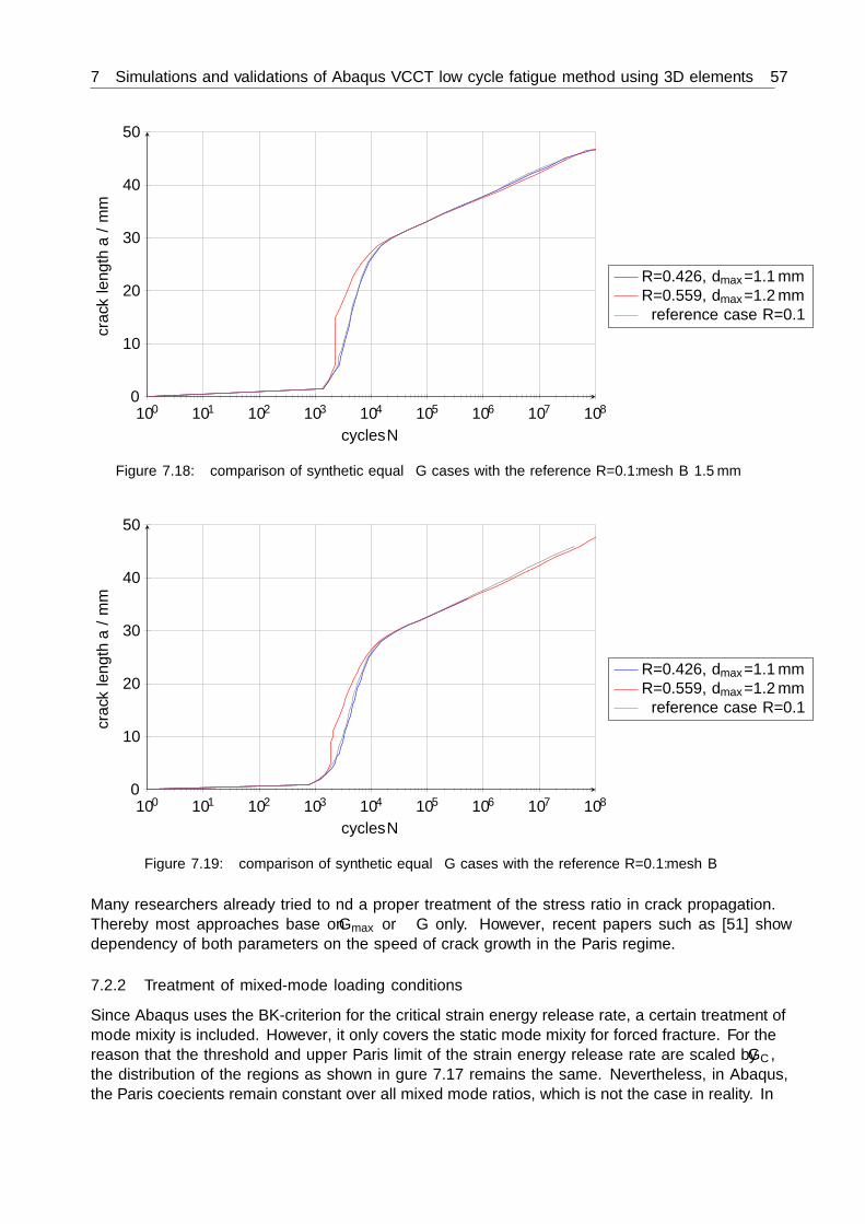
7 Simulations and validations of Abaqus VCCT low cycle fatigue method using 3D elements 57
100 101 102 103 104 105 106 107 1080
10
20
30
40
50
cycles N
crackleng
tha/mm
R=0.426, dmax=1.1mmR=0.559, dmax=1.2mmreference case R=0.1
Figure 7.18: comparison of synthetic equal ∆G cases with the reference R=0.1: mesh B 1.5mm
100 101 102 103 104 105 106 107 1080
10
20
30
40
50
cycles N
crackleng
tha/mm
R=0.426, dmax=1.1mmR=0.559, dmax=1.2mmreference case R=0.1
Figure 7.19: comparison of synthetic equal ∆G cases with the reference R=0.1: mesh B
Many researchers already tried to find a proper treatment of the stress ratio in crack propagation.Thereby most approaches base on Gmax or ∆G only. However, recent papers such as [51] showdependency of both parameters on the speed of crack growth in the Paris regime.
7.2.2 Treatment of mixed-mode loading conditions
Since Abaqus uses the BK-criterion for the critical strain energy release rate, a certain treatment ofmode mixity is included. However, it only covers the static mode mixity for forced fracture. For thereason that the threshold and upper Paris limit of the strain energy release rate are scaled by GC ,the distribution of the regions as shown in figure 7.17 remains the same. Nevertheless, in Abaqus,the Paris coefficients remain constant over all mixed mode ratios, which is not the case in reality. In
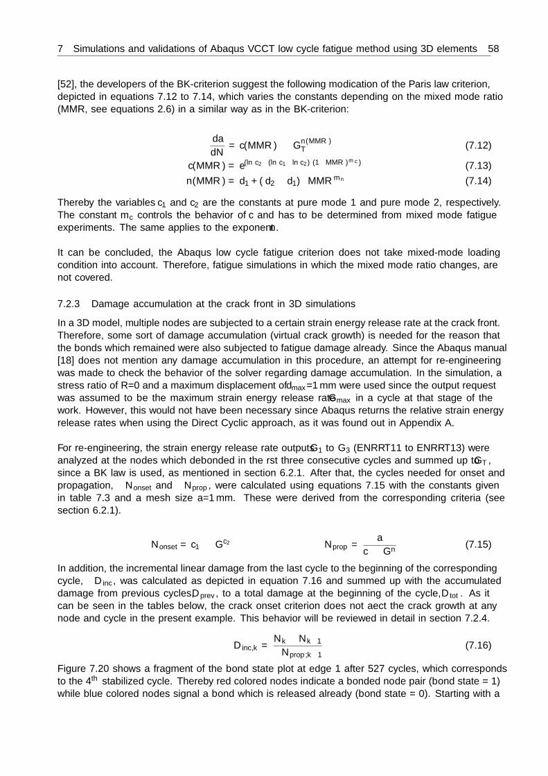
7 Simulations and validations of Abaqus VCCT low cycle fatigue method using 3D elements 58
[52], the developers of the BK-criterion suggest the following modification of the Paris law criterion,depicted in equations 7.12 to 7.14, which varies the constants depending on the mixed mode ratio(MMR, see equations 2.6) in a similar way as in the BK-criterion:
da
dN= c(MMR) ·∆Gn(MMR)
T (7.12)
c(MMR) = e(ln c2−(ln c1−ln c2)·(1−MMR)mc ) (7.13)n(MMR) = d1 + (d2 − d1) ·MMRmn (7.14)
Thereby the variables c1 and c2 are the constants at pure mode 1 and pure mode 2, respectively.The constant mc controls the behavior of c and has to be determined from mixed mode fatigueexperiments. The same applies to the exponent n.
It can be concluded, the Abaqus low cycle fatigue criterion does not take mixed-mode loadingcondition into account. Therefore, fatigue simulations in which the mixed mode ratio changes, arenot covered.
7.2.3 Damage accumulation at the crack front in 3D simulations
In a 3D model, multiple nodes are subjected to a certain strain energy release rate at the crack front.Therefore, some sort of damage accumulation (virtual crack growth) is needed for the reason thatthe bonds which remained were also subjected to fatigue damage already. Since the Abaqus manual[18] does not mention any damage accumulation in this procedure, an attempt for re-engineeringwas made to check the behavior of the solver regarding damage accumulation. In the simulation, astress ratio of R=0 and a maximum displacement of dmax=1mm were used since the output requestwas assumed to be the maximum strain energy release rate Gmax in a cycle at that stage of thework. However, this would not have been necessary since Abaqus returns the relative strain energyrelease rates when using the Direct Cyclic approach, as it was found out in Appendix A.
For re-engineering, the strain energy release rate outputs G1 to G3 (ENRRT11 to ENRRT13) wereanalyzed at the nodes which debonded in the first three consecutive cycles and summed up to GT ,since a BK law is used, as mentioned in section 6.2.1. After that, the cycles needed for onset andpropagation, ∆Nonset and ∆Nprop, were calculated using equations 7.15 with the constants givenin table 7.3 and a mesh size a=1mm. These were derived from the corresponding criteria (seesection 6.2.1).
Nonset = c1 ·∆Gc2 Nprop = a
c ·∆Gn (7.15)
In addition, the incremental linear damage from the last cycle to the beginning of the correspondingcycle, ∆Dinc, was calculated as depicted in equation 7.16 and summed up with the accumulateddamage from previous cycles, Dprev, to a total damage at the beginning of the cycle, Dtot. As itcan be seen in the tables below, the crack onset criterion does not affect the crack growth at anynode and cycle in the present example. This behavior will be reviewed in detail in section 7.2.4.
∆Dinc,k = Nk −Nk−1∆Nprop,k−1
(7.16)
Figure 7.20 shows a fragment of the bond state plot at edge 1 after 527 cycles, which correspondsto the 4th stabilized cycle. Thereby red colored nodes indicate a bonded node pair (bond state = 1)while blue colored nodes signal a bond which is released already (bond state = 0). Starting with a
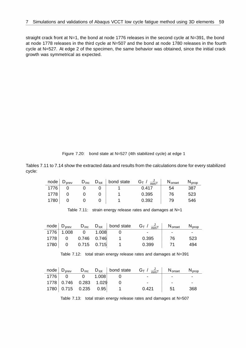
7 Simulations and validations of Abaqus VCCT low cycle fatigue method using 3D elements 59
straight crack front at N=1, the bond at node 1776 releases in the second cycle at N=391, the bondat node 1778 releases in the third cycle at N=507 and the bond at node 1780 releases in the fourthcycle at N=527. At edge 2 of the specimen, the same behavior was obtained, since the initial crackgrowth was symmetrical as expected.
Figure 7.20: bond state at N=527 (4th stabilized cycle) at edge 1
Tables 7.11 to 7.14 show the extracted data and results from the calculations done for every stabilizedcycle:
node Dprev ∆Dinc Dtot bond state ∆GT / Jmm2 ∆Nonset ∆Nprop
1776 0 0 0 1 0.417 54 3871778 0 0 0 1 0.395 76 5231780 0 0 0 1 0.392 79 546
Table 7.11: strain energy release rates and damages at N=1
node Dprev ∆Dinc Dtot bond state ∆GT / Jmm2 ∆Nonset ∆Nprop
1776 1.008 0 1.008 0 - - -1778 0 0.746 0.746 1 0.395 76 5231780 0 0.715 0.715 1 0.399 71 494
Table 7.12: total strain energy release rates and damages at N=391
node Dprev ∆Dinc Dtot bond state ∆GT / Jmm2 ∆Nonset ∆Nprop
1776 0 0 1.008 0 - - -1778 0.746 0.283 1.029 0 - - -1780 0.715 0.235 0.95 1 0.421 51 368
Table 7.13: total strain energy release rates and damages at N=507

7 Simulations and validations of Abaqus VCCT low cycle fatigue method using 3D elements 60
node Dprev ∆Dinc Dtot bond state ∆GT / Jmm2 ∆Nonset ∆Nprop
1776 1.008 0 1.008 0 - - -1778 1.029 0 1.029 0 - - -1780 0.95 0.054 1.004 0 - - -
Table 7.14: total strain energy release rates and damages at N=527
As it can be seen, the bond always releases (=bond state switches to 0), when the linear accumulateddamage reaches a value slightly above 1. Therefore it can be said, that the assumed linear damageaccumulation seems to be considered in this procedure.
7.2.4 Impact of the crack onset criterion
Since both criteria for onset and propagation are depending on ∆G (compare section 7.2.1, inparticular figure 7.17), two cases are possible at a certain ∆G:
� The propagation-only case, in which the number of cycles needed for onset is smaller thanthe number of cycles needed for crack propagation to the next node at the beginning of theanalysis already.
� The onset-propagation case, in which the number of cycles needed for onset is larger thanthe number of cycles needed for crack propagation to the next node.
In the case of the example above in section 7.2.3, where the ENF specimen with the fractureparameters from table 7.3 are used, the behavior of these criteria can be compared by plotting thecycles needed for onset and propagation over ∆G by using equations 7.15:
10−1 100100
101
102
103
104
105
106
107
∆G / Jmm2
cycles
N
NonsetNprop
Figure 7.21: crack onset and propagation criterion for the ENF mode 2 model over ∆G in the Paris regimefor the nodes at the initial crack front
It can be clearly seen, that in the case of the mode 2 ENF model with the present material parametersand mesh size, the onset criterion is smaller than the propagation criterion over the whole Parisregime. Therefore, as already shown in section 7.2.3, the crack onset criterion does not affect the
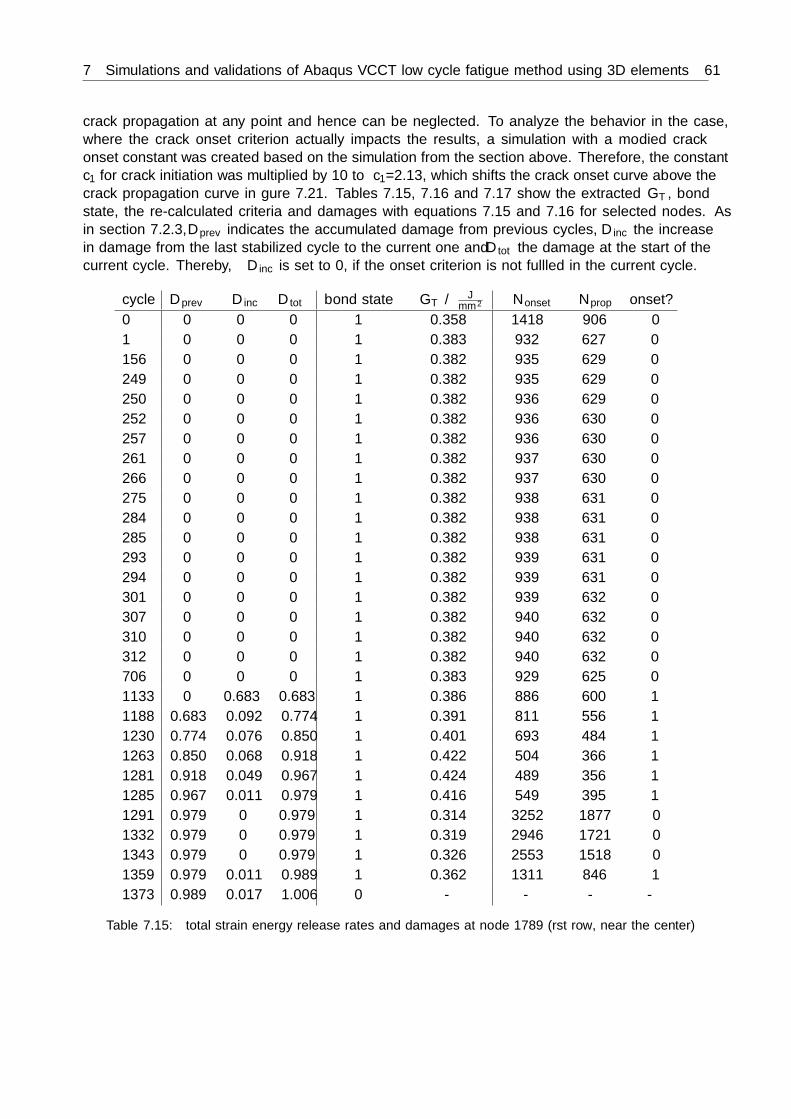
7 Simulations and validations of Abaqus VCCT low cycle fatigue method using 3D elements 61
crack propagation at any point and hence can be neglected. To analyze the behavior in the case,where the crack onset criterion actually impacts the results, a simulation with a modified crackonset constant was created based on the simulation from the section above. Therefore, the constantc1 for crack initiation was multiplied by 10 to c1=2.13, which shifts the crack onset curve above thecrack propagation curve in figure 7.21. Tables 7.15, 7.16 and 7.17 show the extracted ∆GT , bondstate, the re-calculated criteria and damages with equations 7.15 and 7.16 for selected nodes. Asin section 7.2.3, Dprev indicates the accumulated damage from previous cycles, ∆Dinc the increasein damage from the last stabilized cycle to the current one and Dtot the damage at the start of thecurrent cycle. Thereby, ∆Dinc is set to 0, if the onset criterion is not fulfilled in the current cycle.
cycle Dprev ∆Dinc Dtot bond state ∆GT / Jmm2 ∆Nonset ∆Nprop onset?
0 0 0 0 1 0.358 1418 906 01 0 0 0 1 0.383 932 627 0156 0 0 0 1 0.382 935 629 0249 0 0 0 1 0.382 935 629 0250 0 0 0 1 0.382 936 629 0252 0 0 0 1 0.382 936 630 0257 0 0 0 1 0.382 936 630 0261 0 0 0 1 0.382 937 630 0266 0 0 0 1 0.382 937 630 0275 0 0 0 1 0.382 938 631 0284 0 0 0 1 0.382 938 631 0285 0 0 0 1 0.382 938 631 0293 0 0 0 1 0.382 939 631 0294 0 0 0 1 0.382 939 631 0301 0 0 0 1 0.382 939 632 0307 0 0 0 1 0.382 940 632 0310 0 0 0 1 0.382 940 632 0312 0 0 0 1 0.382 940 632 0706 0 0 0 1 0.383 929 625 01133 0 0.683 0.683 1 0.386 886 600 11188 0.683 0.092 0.774 1 0.391 811 556 11230 0.774 0.076 0.850 1 0.401 693 484 11263 0.850 0.068 0.918 1 0.422 504 366 11281 0.918 0.049 0.967 1 0.424 489 356 11285 0.967 0.011 0.979 1 0.416 549 395 11291 0.979 0 0.979 1 0.314 3252 1877 01332 0.979 0 0.979 1 0.319 2946 1721 01343 0.979 0 0.979 1 0.326 2553 1518 01359 0.979 0.011 0.989 1 0.362 1311 846 11373 0.989 0.017 1.006 0 - - - -
Table 7.15: total strain energy release rates and damages at node 1789 (first row, near the center)

7 Simulations and validations of Abaqus VCCT low cycle fatigue method using 3D elements 62
cycle Dprev ∆Dinc Dtot bond state ∆GT / Jmm2 ∆Nonset ∆Nprop onset?
706 0 0 0 1 - - - -1133 0 0 0 1 0.463 277 216 11188 0 0.254 0.254 1 0.503 165 138 11230 0.254 0.305 0.559 1 0.518 137 117 11263 0.559 0.282 0.842 1 0.526 125 108 11281 0.842 0.167 1.009 0 - - - -
Table 7.16: total strain energy release rates and damages at node 1878 (at a=1mm, near edge 1)
cycle Dprev ∆Dinc Dtot bond state ∆GT / Jmm2 ∆Nonset ∆Nprop onset?
3693 0 0 0 1 - - - -3696 0 0 0 1 0.381 962 645 13698 0 0.003 0.003 1 0.456 305 235 13712 0.003 0.059 0.063 1 0.460 291 226 13727 0.063 0.066 0.129 1 0.466 269 211 13742 0.129 0.071 0.200 1 0.469 256 202 13747 0.200 0.025 0.225 1 0.472 248 197 13793 0.225 0.234 0.459 1 0.473 244 194 13885 0.459 0.475 0.934 1 0.477 231 185 13893 0.934 0.043 0.977 1 0.502 166 138 13895 0.977 0.014 0.992 1 0.470 253 200 13899 0.992 0.020 1.012 0 - - - -
Table 7.17: total strain energy release rates and damages at node 3387 (at a=16mm, near the center)
In the case of node 1789, which is located at the initial crack front, the crack onset criterion delaysthe crack propagation. As it can be seen, the re-calculated damage is in agreement with the responseof the bond state.At node 1878, which is the first debonding node pair, that is not located at the initial crack front,the onset criterion is satisfied already. This is also the case at node 3387, which is placed at a cracklength of 16mm. In both cases, the re-calculated damage confirms the behavior of the bond stateagain.Figure 7.22 shows the crack progress of the simulation with modified onset criterion and the refer-ence simulation. As expected, the simulation with modified onset criterion delays the initial crackprogress, but the curve converges to the reference simulation later on.

7 Simulations and validations of Abaqus VCCT low cycle fatigue method using 3D elements 63
100 101 102 103 104 105 106 107 1080
10
20
30
40
50
60
70
cycles N
crackleng
tha/mm
referencemodified onset
Figure 7.22: influence of the onset criterion onto the crack progress
Errors induced by the crack onset criterion
In certain simulations, the criterion for crack onset, which is included in the Abaqus low-cyclefatigue fracture criterion, leads to calculation errors of ∆G2 and ∆G3. This strongly impacts mode2 or mode 3 driven crack propagation.In the following, the behavior is shown in a representative example, which is a modified versionof the setup used in section 7.2.4. Thereby the constant c1 was multiplied by 100 to c1=21.3.Furthermore the synthetic load case R=0.426 from section 7.2.1 was used.Figure 7.23 shows the bond state at 9880 cycles, where red indicates bonded nodes while blue signalsa broken bond. It can be seen, that two bonds remain in the debonded area, namely node 1988(left) and node 2088 (right).
Figure 7.23: bond state at N=9880
In the damage accumulation table 7.18 for node 1988, which is similar to the tables shown insection 7.2.4, it can be seen that with decreasing load due to 3D effects on the crack front, theonset criterion swaps to 0 again, hence blocking further damage accumulation. As a consequence,

7 Simulations and validations of Abaqus VCCT low cycle fatigue method using 3D elements 64
node 1988 and the node behind it, node 2088, form a peninsula until they are undermined andseparated. Since these two nodes are not subjected to the crack front anymore, the strain energyrelease rates in mode 2 and 3 cannot be calculated. However, Abaqus is still able to calculate themode 1 strain energy release rate, which is not sufficient to force debonding in the present mode 2ENF simulation, though.
cycle Dprev ∆Dinc Dtotbondstate
∆G1/ J
mm2
∆G2/ J
mm2
∆G3/ J
mm2
∆GT/ J
mm2∆Nonset ∆Nprop onset?
7737 0 0 0 1 0 0 0 0 - - 07738 0 0 0 1 0 0.415 0 0.415 5567 399 17782 0 0.110 0.110 1 0 0.404 0 0.404 6612 464 17856 0.110 0.159 0.270 1 0 0.406 0 0.406 6413 452 17857 0.270 0.002 0.272 1 0 0.408 0 0.408 6225 440 17894 0.272 0.084 0.356 1 0 0.416 0 0.416 5460 393 17895 0.356 0.003 0.358 1 0 0.480 0 0.480 2215 178 17938 0.358 0.242 0.600 1 0 0.490 0 0.490 1956 160 17966 0.600 0.175 0.776 1 0 0.491 0 0.491 1926 157 17967 0.776 0.006 0.782 1 0 0.499 0 0.499 1741 144 17968 0.782 0.007 0.789 1 0 0.506 0 0.506 1581 132 17969 0.789 0.008 0.796 1 0 0.514 0 0.514 1439 122 17970 0.796 0.008 0.805 1 0 0.521 0 0.521 1320 113 17978 0.805 0 0.805 1 0 0.341 0 0.341 19160 1180 0
7979 0.805 0.001 0.806 1 3.2 ·10−6 QNAN QNAN 3.2 ·
10−61.23 ·1036
9.51 ·1030 0
Table 7.18: total strain energy release rates and damages at node 1988 (third row, near the center, seefigure 7.23)
The behavior of the onset criterion was re-calculated successfully. However, in the Abaqus im-plementation, the criterion uses ∆GT instead of G1,max. This means, the Abaqus implementationgeneralizes the initial model (see section 4.4.2) to mixed mode conditions, which is almost certainlyinsufficient apart from using the relative strain energy release rate instead of the maximum value.In addition, the behavior at node 1789 in the cycles 1291, 1332 and 1343 is physically questionablesince once the onset criterion is fulfilled, it should not affect the propagation anymore.As a conclusion, the current implementation of the criterion for crack onset in the Abaqus lowcycle fatigue criterion remains highly questionable and should be used with care or just excludedby setting the constant c1 to 0.
7.2.5 Behavior at phase-shifted and non-sinusoidal cyclic loadings
The Direct Cyclic algorithm delivers the relative strain energy release rate needed for further cal-culations of the crack growth. To test its robustness and applicability to general load cases, theinitially used sinusoidal loadings were modified in the reference case simulation.
Phase-shifted loadings
At the beginning, different phase shifts t0 were applied to the sine loading of the reference case (seesection 7.1.1), as depicted in figure 7.24:

7 Simulations and validations of Abaqus VCCT low cycle fatigue method using 3D elements 65
0 0.02 0.04 0.06 0.08 0.1 0.12 0.14 0.16 0.18 0.20
0.2
0.4
0.6
0.8
1
time t / s
amplitu
dea(t)
reference case, t0=0st0=-0.05s=+0.15s
t0=+0.05st0=+0.1st0=+0.15s
Figure 7.24: periodic sine loading for R=0.1 with different phase shifts t0
Figure 7.25 shows the resulting output curves of the mode 2 strain energy release rate (ENRRT12)at the first fatigue cycle:
0 0.02 0.04 0.06 0.08 0.1 0.12 0.14 0.16 0.18 0.20
0.1
0.2
0.3
0.4
0.5
time t / s
G2/
Jm
m2
reference case, t0=0st0=-0.05st0=+0.05st0=+0.1st0=+0.15s
Figure 7.25: evolution of the output variable ENRRT12 over a single loading cycle with different phaseshifts t0
The following statements are obtained:
� The maximum relative strain energy release rate ∆Gmax is held till the end of a stabilizedcycle. It occurs when reaching the maximum load.
� The level of the maximum energy release rate is dependent on the position in a cycle whenfacing the same load.
� The relative strain energy release rate output is not increased until the slope of the load isnot negative anymore and the initial value is reached (compare t0=+0.1s).
� The following behavior remains unclear:
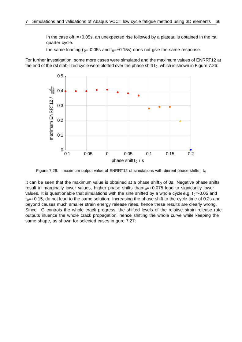
7 Simulations and validations of Abaqus VCCT low cycle fatigue method using 3D elements 66
– In the case of t0=+0.05s, an unexpected rise followed by a plateau is obtained in the firstquarter cycle.
– the same loading (t0=-0.05s and t0=+0.15s) does not give the same response.
For further investigation, some more cases were simulated and the maximum values of ENRRT12 atthe end of the first stabilized cycle were plotted over the phase shift t0, which is shown in Figure 7.26:
−0.1 −0.05 0 0.05 0.1 0.15 0.20
0.1
0.2
0.3
0.4
0.5
phase shift t0 / s
max
imum
ENRRT
12/
Jm
m2
Figure 7.26: maximum output value of ENRRT12 of simulations with different phase shifts t0
It can be seen that the maximum value is obtained at a phase shift t0 of 0s. Negative phase shiftsresult in marginally lower values, higher phase shifts than t0=+0.075 lead to significantly lowervalues. It is questionable that simulations with the sine shifted by a whole cycle, e.g. t0=-0.05 andt0=+0.15, do not lead to the same solution. Increasing the phase shift to the cycle time of 0.2s andbeyond causes much smaller strain energy release rates, hence these results are clearly wrong.Since ∆G controls the whole crack progress, the shifted levels of the relative strain release rateoutputs influence the whole crack propagation, hence shifting the whole curve while keeping thesame shape, as shown for selected cases in figure 7.27:

7 Simulations and validations of Abaqus VCCT low cycle fatigue method using 3D elements 67
100 101 102 103 104 105 106 107 1080
10
20
30
40
50
cycles N
crackleng
tha/mm
reference case, t0=0st0=-0.05st0=+0.05st0=+0.1s
Figure 7.27: comparison of crack propagation curves resulting from different phase shifts
Non-sinusoidal cyclic loadings
In the next step, loading cases in which multiple nested cycles in a given cycle duration or pointsof discontinuity occur, were evaluated. Latter refers to loadings with swapping load vector inmode 2 (0 < R < -∞), since a single loading cycle can be interpreted as two individual halfcycles due to the fact that the acting shear stresses affect the crack propagation in positive andnegative direction (linear-elastic material). This also shows multiple peaks of the maximum strainenergy release rates. Therefore, a simulation using R=-1 with scaled maximum displacement forthe reason of comparability to the reference case concerning ∆Gmax was created with the findingsfrom section 7.2.1. Note that these simulations must be considered synthetic since in the currenttest setup, no tension forces can be applied. In addition, a second simulation using an amplitudecurve which represents R=-1 but with a mirrored second half-cycle was created to test the treatmentof a point of discontinuity in the displacement function. Eventually a simulation using R=0 andtwo cycles was built up, since this simulation shows peaks with the same maximum relative strainenergy release rate. The corresponding amplitude curves are shown in figure 7.28:

7 Simulations and validations of Abaqus VCCT low cycle fatigue method using 3D elements 68
0 0.02 0.04 0.06 0.08 0.1 0.12 0.14 0.16 0.18 0.2−1
−0.5
0
0.5
1
time t / s
amplitu
dea(t)
reference caseR=-1
R=-1 absoluteR=0, two cycles
Figure 7.28: periodic loadings
For the reason of convergence problems in the simulation with R=-1 and absolute amplitude, the Dir-ect Cyclic control parameters for displacement corrections (3rd and 5th entrance, see section 7.1.4),which were set to 1 · 10−3 in the reference case, were increased to 5 · 10−3 (compare Appendix D).This is caused by the point of discontinuity in the function, which complicates the search for aproper Fourier representation. In Figure 7.29 shows the evolution of G2 over the first stabilizedcycle. As it can be seen, the response of G2 differs at the beginning when comparing R=0 withR=-1, but reaches about the same level at 1/4 of the cycle, as expected in the case without phaseshift. In the case of R=-1 with the mirrored second half cycle, the maximum strain energy releaserate reaches a lower level.
0 0.02 0.04 0.06 0.08 0.1 0.12 0.14 0.16 0.18 0.20
0.1
0.2
0.3
0.4
0.5
time t / s
G2/
Jm
m2
reference caseR=-1
R=-1, absoluteR=0, two cycles
Figure 7.29: ∆G2,max over a single loading cycle
Figure 7.30 depicts the resulting crack propagation curves. Thereby the curve from R=0 overlapswith the reference case. As a result of lower ∆GT,max, the curve from R=-1 and absolute amplitudeis shifted to the right by about factor 2, which means that the crack propagates at half velocity.

7 Simulations and validations of Abaqus VCCT low cycle fatigue method using 3D elements 69
100 101 102 103 104 105 106 107 1080
10
20
30
40
50
cycles N
crackleng
tha/mm
reference caseR=-1
R=-1, absoluteR=0, two cycles
Figure 7.30: comparison of the crack propagation curves
In summary, the levels of the maximum relative strain energy release rate outputs are influencedby the position of the maximum loading in the cycle. When it occurs at 1/4 of the cycle duration,which corresponds to a simple sine loading, the relative strain energy release rate outputs coincidewith the level from static calculations, while later occurrence causes lower outputs. Multiple loadpeaks in a cycle seem not to be detected. However, the case of R=-1 returns a slightly higher outputthan R=0 despite having the same position of the (first) maximum load.
7.2.6 CPU-parallelization, cycle limit
Due to the high calculation times needed for simple models already, the effects and efficiency ofCPU-parallelization were tested. Therefore, a simulation with mesh B 2mm, automatic contactstabilization and the reference loading case of R=0.1 was started with 1 and 3 CPU cores on the samecomputer and the results were compared to each other. Figures 7.31 depict the crack propagationcurves for considered node sets. It can be seen, that CPU parallelization impacted the results onthe edges in the region after passing the point of load entry in the middle of the specimen. Due toCPU-parallelization, the calculation time decreased by 40%.
100 1050
15
30
45
cycles N
crackleng
tha/mm
100 1050
15
30
45
cycles N100 105
0
15
30
45
cycles N
1 CPU3 CPUs
Figure 7.31: comparison of the crack propagation curves regarding CPU-parallelization: edge 1 (left), center(mid) and edge 2(right)

7 Simulations and validations of Abaqus VCCT low cycle fatigue method using 3D elements 70
In another attempt, a simulation with smaller mesh size was taken (mesh A, R=0, dmax=1mm,viscosity=1 ·10−6). Thereby, simulations with 1, 3 and 4 CPUs were compared to each other. Afterpassing the line of load introduction, small deviations arise, which decay with rising crack length,as it can be seen in figures 7.32. Compared to the simulation with only 1 CPU, the calculation timedecreased by about 30% in the case of 3 CPUs and by 31% in the case of 4 CPUs.
100 1050
25
50
cycles N
crackleng
tha/mm
100 1050
25
50
cycles N100 105
0
25
50
cycles N
1 CPU3 CPUs4 CPUs
Figure 7.32: comparison of the crack propagation curves regarding CPU-parallelization: edge 1 (left), center(mid) and edge 2(right)
Tests at the "Mach" mainframe of the University have shown, that excessive parallelization with 8cores and more does not decrease the calculation time significantly. Therefore, it is not recommendedto use more than 3 CPUs, since the parallelization does not work that well using the Direct Cyclicapproach. However, high clock rates and fast storage devices significantly accelerate the calculation.
In addition, tests with a very high number of cycles have shown, that the calculation crashes aboveabout 2 · 109 cycles, since the step time jumps to negative values there. Therefore it seems that thecycle number is a 32bit integer. A workaround for simulating even a higher number of cycles, anadditional equal Direct Cyclic step can be created.

7 Simulations and validations of Abaqus VCCT low cycle fatigue method using 3D elements 71
7.3 Guidelines for implementation and input parameters
In the course of the work, several parameters were found for successful, efficient fatigue crack growthsimulations using the Abaqus VCCT low cycle fatigue analysis. These are listed in the following:
� For accurate results, especially when using 3D models, solid elements are recommended overcontinuum shell elements, due to overestimation of the strain energy release rates and pos-sible convergence problems [39] when using latter. For bending problems, linear elementswith incompatible node formulation are preferred due to their significantly better bendingrepresentation.
� Element sizes of 0.1 ≤ ∆a/h ≤ 1 are recommended for composites according to [19]. Fur-thermore until the treatment of different element sizes over the estimated crack surface isvalidated, it should be kept constant.
� Sinusoidal fatigue loadings without phase shift are recommended for proper calculation of thestrain energy release rates via the Abaqus Direct Cyclic Approach (compare section 7.2.5).
� According to current knowledge, crack propagation over the line of load introduction shouldbe avoided and if not, evaluated with care (compare section 7.1.5 and Appendix C).
� The crack onset criterion should be excluded in 3D simulations since it can lead to calcula-tion errors (see section 7.2.4). Furthermore its implementation is questionable anyway since∆GT is used instead of G1,max, which is taken in in the original proposal of the theory (seesection 6.2.1).
� According to Krueger [49], the maximum number of Fourier terms (50) are recommendedfor accurate results. However, tests have shown, that the automatic incremental definition iscapable of returning highly accurate results at slightly decreased calculation times, too (seeAppendix D).
� The Direct Cyclic control parameters are essential for convergence, accuracy and calculationtime and hence have to be set with care. In cases where convergence is not given whenusing the default parameters, these should be increased step-by-step. In the present case,the parameter which is responsible for the residual displacement criterion was significantlyincreased to deactivate the corresponding criterion. Furthermore in Appendix D, modifyingthe other parameters was tested.
� Stabilization or viscous regularization is usually not required. When using fixed time steps,which is required in non-dissipative simulations, the release tolerance has no effect.
� In a single Direct Cyclic step, only 2 · 109 cycles are possible. For larger numbers, multiple,equal Direct Cyclic steps have to be created.
7 Simulations and validations of Abaqus VCCT low cycle fatigue method using 3D elements 72
7.4 Summary of the assessment regarding fatigue delamination under cyclicloading
The Abaqus VCCT low cycle fatigue method offers the following capabilities and advantages:
� the approach is based on physical assumptions
� the parameters needed can be obtained from classical fracture mechanics tests
� the effect of stress ratio is covered in the way that equal values of the relative total strainenergy release rate return equal rates of crack growth (see section 7.2.1)
� crack onset, which is needed for e.g. ply drop-offs, is included
� in 3D simulations, the virtual crack growth of the non-debonding nodes at the crack front istaken into account (see section 7.2.3)
However, the method still has clear limits and drawbacks, which are:
� Simulations with changing mixed-mode ratio (MMR) are not covered in the low cycle fatiguecriterion due to the 1D implementation of Paris law. Therefore, it is only applicable to verysimple applications such as typical fracture mechanics specimens.
� The crack onset criterion’s implementation is questionable, since the equivalent relative strainenergy release rate ∆G is taken instead of the maximum mode 1 strain energy release rateG1,max. Furthermore it can lead to unreasonable calculation errors in 3D crack fronts.
� The method does not work properly when large stiffness differences between the layers occur[53].
� Certain simulations in which the crack passes the line of load introduction show unreasonablestrain energy release rates in certain modes after passing it. Further research is recommendedregarding this behavior.
� The Direct Cyclic step is very sensitive to the applied load amplitude curve. A simple phaseshift can significantly change the results. For the reason of the Fourier series representationof the displacement and residual vectors, points of discontinuity lead to convergence problemsor unreasonable results.
� Due to the VCCT implementation, an initial crack and a predefined crack surface is needed.Furthermore a more or less serrated crack propagation is obtained, depending on the meshsize. However, to damp this behavior, which is especially observable in 2D simulations, thedebonding of node pairs can be modeled gradually, see section 7.1.2 and [54].
� Calculation times are very high for simple models already, hence complex 3D geometries wouldneed an unbearable amount of computational resources.
For an application to the composite rim, which was used as the motivation for this work, mixedmode treatment would have been needed. Furthermore, crack initiation is not covered by VCCT,which is another major drawback. In addition, the erratic behavior of the Direct Cyclic algorithmfor phase shifted and more general loading functions is not clear and hence a possible source oferrors. Eventually, the calculation times would have become unbearable. Therefore, no simulationsof the composite rim were performed.

8 Conclusions and future work 73
8 Conclusions and future work
8.1 Research goals and performed work
The aim of this work was to give an overview of the available modeling techniques for fatigue damageof laminated composite structures with a focus on interlaminar damage. Therefore, an extensivereview of methods to describe the complex fatigue behavior of laminated composite materials wasmade. In a second step, promising approaches of certain modeling techniques in finite elementpackages - namely from Siemens Samtech Samcef and 3DS Abaqus - were further investigated andassessed regarding its capabilities and limitations in their implementation, if already included in thecorresponding finite element code. In addition, guidelines for proper implementation were derivedbased on experience.
8.2 Conclusions and recommendations for future work
Fatigue of laminated composite materials is still at the very beginning of its development sinceeven the static behavior is not fully clarified at the moment. This results from the complex damagemechanisms which occur due to multiple constituents of this material. In early attempts, S/N-curveapproaches from metals were used to describe damage in laminates. However, since laminated com-posites can be varied in their ply stacking sequence, as well as their fiber and matrix types, animmense amount of testing is needed. Moreover, these models do not consider the measurable stiff-ness degradation during fatigue life, which causes stress redistribution in the structural componentduring fatigue life.Other fatigue life approaches focus on the residual mechanical properties such as strength or stiffness.Especially the residual stiffness approaches seem to be very promising since stiffness can be measuredby non-destructive testing methods besides its characteristic behavior of exhibiting three differentstages (compare figure 5.2).Compared to laminate based modeling, ply level modeling represents an alternative technique.This method applies a fatigue law directly to the individual plies to model intralaminar damage. Toinclude interlaminar fatigue damage, these methods are usually combined with fracture mechanicsand continuum damage mechanics methods - namely cohesive zone methods. However, most of theseply based models do not consider the interactions between intralaminar and interlaminar matrixfailure. Furthermore, as determined in section 7.2 for VCCT for example, these methods are stillvery limited and inefficient in calculation.The most promising intralaminar composite fatigue models are progressive damage models, whichuse a continuously rising damage variable to represent the damage state of the laminas or thelaminate. Stiffness reduction is calculated according to the arising damage. To include stressredistributions, the FE-model is recalculated after a certain increase in damage. However, thesemodels need many input parameters and are still in an early stage of development.In the last years, new micromechanical approaches emerged, primarily for static strength. Thesemodels focus on a representative volume element, describing the smallest possible repeating unit ofa certain lamina or laminate, in which the physical behavior is described. The resulting responsecan be homogenized in a CDM approach and used for macroscopic application further on. Thisprocedure is called multi-scale modeling. According to the author, these models should be partic-ularly suitable for the derivation of fatigue properties. The following multi-scale fatigue procedurewould be conceivable for an applicable approach:
� For a fundamental understanding of the occurring damage mechanisms considering interac-tions between intra- and interlaminar damage, a micromechanics model representing the lam-inate is suggested. Furthermore its in-plane dimensions should be sufficiently large to coverall damage mechanisms, including micro-buckling in compression. Thus, the accurate fatigue

8 Conclusions and future work 74
behavior of the matrix, the fiber and the interface should be represented by input parameters,as they are intrinsic and the cause of all damage appearance.
� The statistical nature of the main material parameters and the production tolerances shouldbe evaluated carefully and considered in the micromechanics model to include the evolution ofdamages in a statistical manner. Thus, an accurate classification of manufacturing tolerances isrecommended since even small change in the fiber angle or fiber waviness cause high deviationsin the material response and damage mechanisms.
� From the statistical micromechanics model, continuous residual stiffness and residual strengthevolution curves and their probability can be derivated for certain loading conditions andstates of damage. These can be calculated beforehand and stored in databases.
� For finite element modeling of structural elements, shell and continuum shell elements shouldbe preferred over solid elements and further adapted to the composite’s needs due to theircomputational efficiency and accurate representation of thin structures. As in other progressivedamage techniques, the structural response and damage state should be derived incrementallyat certain time steps until failure.
� The whole procedure should be developed for flat structures first and extended to curvedstructures in a next step.
� In service, the remaining stiffness of a structure could be monitored within a structural healthmonitoring (SHM) system, since the remaining fatigue life of a structure can be accuratelyestimated from that remaining stiffness.
For this presented approach, extensive work in the field of micromechanics and deep understandingof the elemental behavior, especially of the polymer matrix and the fiber-matrix interface, is needed.Therefore, existing testing methods for each individual materials have to be evaluated regardingtheir applicability for determining the data required in a micromechanical model and, if necessary,modified. In addition, the statistical behavior of each constituent and input parameter has to bedetermined - starting from the intrinsic material behavior up to the manufacturing of the structuralcomponent - since all these influences sum up. This may better explain the very high scatter ofmaterial tests of laminated composites.
As it can be seen in the present work, the complex fatigue behavior of composite materials is stillan unsolved question. This often leads to significant oversizing and improper design despite hightesting costs, which impairs the immense potential for lightweight structures of composite materials.Therefore, despite the big challenge due to the high complexity, further fundamental research formore optimized laminated composite structures is desirable to eventually exploit the performanceof laminated composite materials.

Literature 75
References[1] Wiedemann, J.: Leichtbau: Elemente und Konstruktion. Springer-Verlag, 2007.[2] Schuermann, H.: Konstruieren mit Faser-Kunststoff-Verbunden. Springer, 2007.[3] Galucio, A.; Jetteur, P; Trallero, D and Charles, J.: ‘Toward numerical fatigue pre-
diction of composite structures: application to helicopter rotor blades’. In: 3rd ECCOMASThematic Conference on Mechanical Response of Composites. Vol. 94. 2011.
[4] Putnam, T. W.: X-29 flight-research program. 1984.[5] Shirk, M. H.; Hertz, T. J. and Weisshaar, T: ‘Aeroelastic tailoring-theory, practice, and
promise.’ In: J. AIRCRAFT. 23.1 (1986), pp. 6–18.[6] Griffith, A. A.: ‘The Phenomena of Rupture and Flow in Solids’. In: Philosophical Trans-
actions of the Royal Society of London. Series A, Containing Papers of a Mathematical orPhysical Character. 1920.
[7] Orowan, E.: ‘Fracture and Strength of Solids’. In: Rep. Progr. Phys. 185 (1948).[8] Gross, D. and Seelig, T.: Bruchmechanik. 6. Auflage. 2016.[9] Sharpe, W. N.: Handbook of Experimental Solid Mechanics. 2008. Chap. 5.
[10] Roylance, D.: ‘Introduction to fracture mechanics’. In: Massachusetts Institute of Techno-logy, Cambridge (2001).
[11] Benzeggagh, M. L. and Kenane, M.: Measurement of mixed-mode delamination fracturetoughnesses of unidirectional glass/epoxy composites with mixed-mode bending apparatus. re-port. Université de Technologie de Compiègne, 1996.
[12] Barbero, E. J.: Introduction to Composite Materials Design. Ed. by Edition, S. 2011.[13] Denkendorf, I.: Hochleistungsfasern für Verbundwerkstoffe. 2015.[14] Campbell, F.: Introduction to Composite Materials. ASM International, 2010.[15] Puck, A.: Festigkeitsanalyse von Faser-Matrix-Laminaten. 1996.[16] Khashaba, U.: Delamination in drilling GFR-thermoset composites. 2003.[17] Hognestad, G.: ‘The use of C-shaped specimens to investigate the interlaminar fracture of
woven composite laminates’. In: Journal of Strain Analysis Vol 30 No 2 1995 (1995).[18] Simulia, D.: Abaqus 6.14 User Manual. 2015.[19] Krueger, R.: The Virtual Crack Closure Technique: History, Approach and Applications.
ICASE, Hampton, Virginia. 2002.[20] Dugdale, D. S.: ‘Yielding of steel sheets containing slits’. In: Journal of the Mechanics and
Physics of Solids 8.2 (1960), pp. 100–104.[21] Barenblatt, G. I.: ‘The mathematical theory of equilibrium cracks in brittle fracture’. In:
Advances in applied mechanics 7 (1962), pp. 55–129.[22] LS-Dyna: LS-Dyna Keyword User’s Manual Volume II Material Models. Version R7.0. 2013.[23] Turon, A.; Dávila, C. G.; Camanho, P. P. and Costa, J.: ‘An engineering solution for
using coarse meshes in the simulation of delamination with cohesive zone models’. In: (2005).[24] Radaj, D. and Vormwald, M.: Ermüdungsfestigkeit. 2007.[25] Rösler, J.; Harders, H. and Bäker, M.: Mechanisches Verhalten der Werkstoffe. 2012.[26] Vassilopoulos, A. and Keller, T.: Fatigue of Fiber-reinforced Composites. 2011.

Literature 76
[27] Hammer, F. and Leopold, J.: Großschaden an einem 300MW Dampfturbosatz. 1988.[28] Wiedemann, J: Leichtbau Elemente und Konstruktion. 2007.[29] Murri, G. B.; Salpekar, S. A. and O’Brien, T. K.: ‘Fatigue delamination onset prediction
in unidirectional tapered laminates’. In: Composite Materials: Fatigue and Fracture (ThirdVolume). ASTM International, 1991.
[30] O’Brien, T. K.; Johnston, W. M. and Toland, G. J.: ‘Mode II interlaminar fracturetoughness and fatigue characterization of a graphite epoxy composite material’. In: (2010).
[31] Paris, P. C. and Erdogan, F.: ‘A critical analysis of crack propagation laws’. In: ASME.1963.
[32] Walker, K: ‘The effect of stress ratio during crack propagation and fatigue for 2024-T3 and7075-T6 aluminum’. In: Effects of environment and complex load history on fatigue life. ASTMInternational, 1970.
[33] Vassilopoulos, A. P.; Manshadi, B. D. and Keller, T.: ‘Piecewise non-linear constant lifediagram formulation for FRP composite materials’. In: International journal of fatigue 32.10(2010), pp. 1731–1738.
[34] Philippidis, T. and Vassilopoulos, A.: ‘Fatigue design allowables for GRP laminates basedon stiffness degradation measurements’. In: Composites science and technology 60.15 (2000),pp. 2819–2828.
[35] Hashin, Z. and Rotem, A.: ‘A fatigue failure criterion for fiber reinforced materials’. In:Journal of composite materials 7.4 (1973), pp. 448–464.
[36] Tsai, S. W. and Wu, E. M.: ‘A general theory of strength for anisotropic materials’. In:Journal of composite materials 5.1 (1971), pp. 58–80.
[37] Plumtree, A and Cheng, G.: ‘A fatigue damage parameter for off-axis unidirectional fibre-reinforced composites’. In: International Journal of fatigue 21.8 (1999), pp. 849–856.
[38] Degrieck, J. and Van Paepegem, W.: ‘Fatigue damage modeling of fibre-reinforced com-posite materials: Review’. In: Applied Mechanics Reviews 54.4 (2001), pp. 279–300.
[39] Camanho, P. P. and Hallett, S. R.: Numerical modelling of failure in advanced compositematerials. Woodhead Publishing, 2015.
[40] Bak, B. L.; Sarrado, C.; Turon, A. and Costa, J.: ‘Delamination under fatigue loads incomposite laminates: a review on the observed phenomenology and computational methods’.In: Applied Mechanics Reviews 66.6 (2014), p. 060803.
[41] Carrella-Payan, D et al.: ‘Implementation of fatigue model for unidirectional laminatebased on finite element analysis: theory and practice’. In: Frattura ed Integrità Strutturale 38(2016), p. 184.
[42] Carrella-Payan, D et al.: Implementation of Fatigue Model for UD Laminate based onFEA: Theory and Practice. 2016.
[43] Van Paepegem, W: ‘Development and finite element implementation of a damage model forfatigue of fibre-reinforced polymers’. PhD thesis. University of Ghent, 2002.
[44] Brokate, M.; Dreßler, K. and Krejci, P.: Rainflow Counting and Energy Dissipation forHysteresis Models in Elastoplasticity. report. University of Kaiserslautern, 1996.
[45] Van Paepegem, W. and Degrieck, J.: ‘Calculation of damage-dependent directional failureindices from the Tsai–Wu static failure criterion’. In: Composites science and technology 63.2(2003), pp. 305–310.

Literature 77
[46] Van Paepegem, W. and Degrieck, J.: ‘Simulating damage and permanent strain in com-posites under in-plane fatigue loading’. In: Computers and structures 83.23 (2005), pp. 1930–1942.
[47] Bruyneel, M. et al.: Calculating Fatigue and Fatigue Failure of Structures. US Patent App.14/273,781. 2014.
[48] Krueger, R.: Development of a benchmark example for delamination fatigue growth predic-tion. 2010.
[49] Krueger, R.: ‘Development and application of benchmark examples for mode II staticdelamination propagation and fatigue growth predictions’. In: (2011).
[50] Krueger, R.: ‘An approach to assess delamination propagation simulation capabilities incommercial finite element codes’. In: (2008).
[51] Khan, R.; Alderliesten, R.; Badshah, S. and Benedictus, R.: ‘Effect of stress ratio ormean stress on fatigue delamination growth in composites: critical review’. In: CompositeStructures 124 (2015), pp. 214–227.
[52] Kenane, M; Azari, Z; Benmedakhene, S and Benzeggagh, M.: ‘Experimental develop-ment of fatigue delamination threshold criterion’. In: Composites Part B: Engineering 42.3(2011), pp. 367–375.
[53] Krueger, R.; Shivakumar, K. N. and Raju, I. S.: ‘Fracture Mechanics Analyses for InterfaceCrack Problems-A Review’. In: 54th AIAA/ASME/ASCE/AHS/ASC Structures, StructuralDynamics, and Materials Conference. 2013, p. 1476.
[54] Bisagni, C.; Brambilla, P. and Bavila, C. G.: Modeling Delamination in Postbuckled Com-posite Structures Under Static and Fatigue Loads. 2013.

Appendix 78
Appendix A Additional information to the strain energy release rate outputs
In the course of the work, it was found out that the Abaqus manual [18] gives wrong informationabout the energy release rate outputs in the direct cyclic analysis in combination with the lowcycle fatigue criterion. According to the definition in "Output variables", chapter 11.4.3 - Crackpropagation analysis in the Abaqus Analysis User’s Guide, the (current) strain energy release rate isdisplayed using the VCCT, enhanced VCCT or low-cycle fatigue criterion. Furthermore, in chapter6.2.7 - Low-cycle fatigue analysis using the direct cycle approach, no additional information isprovided regarding the outputs. However, using the direct cyclic approach in combination with thelow cycle criterion and VCCT crack growth, the strain energy release rate outputs ENRRT give themaximum ∆G = Gmax −Gmin to the corresponding increment in a cycle. This statement is provedin the following lines.
With the findings from section 7.2.1, load cases with different stress ratios, minimum and maximumdisplacements but same relative strain energy release rate ∆G could be created, as depicted infigure A.1:
0 0.02 0.04 0.06 0.08 0.1 0.12 0.14 0.16 0.18 0.20
0.2
0.4
0.6
0.8
1
1.2
time t / s
amplitu
dea(t)
reference caseR=0, dmax=0.995mmR=0.426, dmax=1.1mm
Figure A.1: periodic sine loading with equal ∆G
In figure A.2, the resulting mode 2 strain energy release rate outputs (ENRRT12) are plotted overthe first stabilized cycle. In addition, levels with the maximum energy release rates for all threecases and the relative strain energy release rate over the cycle were added.

Appendix 79
0 0.02 0.04 0.06 0.08 0.1 0.12 0.14 0.16 0.18 0.20
0.1
0.2
0.3
0.4
0.5
0.6
time t / s
G2/
Jm
m2
Gmax at R=0.1Gmax at R=0.426Gmax=∆G at R=0
reference caseR=0, dmax=0.995mmR=0.426, dmax=1.1mm
Figure A.2: evolution of G2 over a single loading cycle with different loadings of equal ∆G
All of the output curves converge to Gmax of R=0, which corresponds to ∆G in all loadings. Sincethe overlap occurs at 1/4 of the cycle, which coincides with the point of maximum displacement,it may be assumed that these outputs provide the maximum ∆G from the start of a cycle untilthe current increment. However, this is also influenced by the point of maximum displacement in acycle, as described in section 7.2.5.
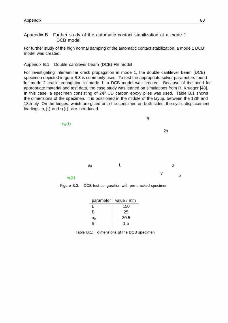
Appendix 80
Appendix B Further study of the automatic contact stabilization at a mode 1DCB model
For further study of the high normal damping of the automatic contact stabilization, a mode 1 DCBmodel was created.
Appendix B.1 Double cantilever beam (DCB) FE model
For investigating interlaminar crack propagation in mode 1, the double cantilever beam (DCB)specimen depicted in figure B.3 is commonly used. To test the appropriate solver parameters foundfor mode 2 crack propagation in mode 1, a DCB model was created. Because of the need forappropriate material and test data, the case study was leaned on simulations from R. Krueger [48].In this case, a specimen consisting of 24 0° UD carbon epoxy plies was used. Table B.1 showsthe dimensions of the specimen. It is positioned in the middle of the layup, between the 12th and13th ply. On the hinges, which are glued onto the specimen on both sides, the cyclic displacementloadings, ~uu(t) and ~ul(t), are introduced.
~uu(t)
xy
z
B
L
2h
a0
~ul(t)
Figure B.3: DCB test configuration with pre-cracked specimen
parameter value / mmL 150B 25a0 30.5h 1.5
Table B.1: dimensions of the DCB specimen

Appendix 81
Model description
Figure B.4 shows the simplified model used for the simulations. Since the sections behind the hingesdo not exhibit transverse forces, they are unloaded and hence can be neglected.
~ul(t) xy
z
B
a0 L
2h
bonded face
~uu(t)
δ
Figure B.4: simplified DCB model
Material properties
The material properties of the lamina and the 0°/0° interface properties were taken from [48].Table B.2 depicts the lamina properties whereas the interface properties are depicted in table B.3.The latter are divided into static fracture properties using a BK law on the left, delamination growthonset coefficients in the middle and Paris law coefficients for delamination propagation on the right.
E1 E2 = E3 ν12 = ν13 ν23 G12 = G13 G23139.4GPa 10.16GPa 0.3 0.436 4.6GPa 3.54GPa
Table B.2: material properties for the graphite epoxy lamina used
G1C G2C = G3C η c1 c2 Gth c n
0.17J/mm² 0.49J/mm² 1.62 2.8 10−9 -12.415 0.06J/mm² 2.44 106 10.61
Table B.3: fracture parameters for graphite epoxy 0°/0° interface used
Simulation steps
Equally to the ENF model in section 7.1.1, the same solver, steps and parameters, as depicted intable 7.4, were used. As a result of a loading frequency of 10Hz, a single cycle was divided into100 increments each. Regarding the direct cyclic control parameters, these were set according toKrueger’s simulation in [48]. Thereby, the ratio of the maximum residual coefficients to the timeaveraged force CRαn, was set to 100, which means that the criterion was turned off. The othercontrol parameters were kept at default values.

Appendix 82
VCCT interaction
The interface was modeled in the same way as in the ENF specimen, which is described in sec-tion 7.1.1. Thereby the material parameters were taken from table B.3.
Boundary conditions and displacement loadings
At the idealized lines of the hinges (green lines in figure B.4), translation was locked in x- andy-direction. In the static step, a displacement of δmax/2 = 0.00067mm was applied on each hinge incrack opening z-direction, respectively. In the direct cyclic fatigue step, periodic sine loadings witha frequency of 10Hz were applied in crack opening z-direction each. As a result, the same approachwas used as in the ENF model shown in section 7.1.1, except for a doubled angular frequency of62.832Hz. Equations B.1 and B.2 depict the corresponding displacement vectors.
~uu(t) = ~du · a(t) ~du =
00
δmax/2
mm (B.1)
~ul(t) = ~dl · a(t) ~dl =
00
−δmax/2
mm (B.2)
Element type, node sets for evaluation
As in the ENF model (section 7.1.1), linear hexahedral elements with incompatible mode formulationwere used since less elements are needed through the thickness of each stack then. The same appliesto the node sets for evaluation (section 7.1.1).
Appendix B.2 Setting of the simulations
The mesh for the DCB model was modeled in a similar way as mesh B, which can be found insection 7.1.5. Figure B.5 shows the partitioning of a stack. Thereby the less important partitionsA with a length of a = 20.5mm and C with a length of c = 69.5mm were assigned a coarse mesh inlength direction whereas in partition B with a remaining length of 60mm, a finer mesh was used.Table B.4 depicts the number of elements over the partitions and the resulting element sizes.
a c
h
Lx
z
yA CB
Figure B.5: partitioning of the DCB model

Appendix 83
number of elements resulting element sizepartition A 7 ∼3mmpartition B 48 1.25mmpartition C 23 ∼3mmwidth B 20 1.25mmheight H 2 0.75mm
Table B.4: element data in the mesh B models
In figure B.6 the resulting mesh is shown. As in the visualizations of the ENF meshes, the red areaindicates the bonded nodes of the VCCT contact. It can be seen that the mesh refinement is drawnbeyond the initial crack front for the reason of better calculation of the bending deformation nearthe crack tip.
Figure B.6: mesh of the DCB model
The same solver parameters as in the ENF model were used. Two cases were created: one withautomatic contact stabilization and one with very little manual contact stabilization, as suggestedin [49].
Appendix B.3 Results and discussion
Figure B.7 shows the center crack propagation curve of these two cases. It can be seen that thesimulation using constant stabilization follows Krueger’s semi-analytical benchmark curve from [48].The overestimation is induced by the very low number of elements over the thickness. In the case ofautomatic stabilization, the crack propagates significantly too slow due to notably reduced relativemode 1 strain energy release rates ∆G1. This is induced by the high normal damping of theautomatic contact stabilization.

Appendix 84
100 101 102 103 104 105 106 107 1080
2
4
6
8
10
12
cycles N
crackleng
tha/mm
automatic stabilizationconstant stabilization 10−6
benchmark curve
Figure B.7: comparison of the crack propagation curves
0 1 2 3 4 5 6 7 8 9 100.05
0.1
0.15
0.2
0.25
crack length a / mm
∆G
1/
103
J m2
automatic stabilizationconstant stabilization 10−6
Figure B.8: comparison of ∆G1 over the crack length
Comparison of the increase of static dissipation energy to the maximum strain energy in a cycleshow that these have the same order of magnitude in the case of automatic stabilization, whereasusing constant stabilization, ALLSD/ALLSE is under 1ppm. The excessive normal damping whenusing automatic stabilization can be even seen in the deformation, as depicted in figure B.9. There,the end of the red line indicates the crack front.

Appendix 85
Figure B.9: upper figure: deformation with low constant stabilization; lower figure: deformation usingautomatic stabilization

Appendix 86
Appendix C ENF Simulations using an undistorted mesh and non simplifiedgeometry
To inspect the effect of mesh distortion in Mesh B in the ENF model and a possible influence ofthe unloaded regions, two similar models, one full size model and one with the unnecessary regionscropped, were created with imperial mesh size dimensioning.In mesh B, the upper stack is slightly distorted because of the imperial sized point of load entranceat the upper surface combined with a mesh size of 1mm in the significant region of the VCCTcontact at the lower surface.
Appendix C.1 Setting of the simulations
Figure C.10 depicts the full size model while in the simplified model, the mesh was cropped at thesupports (red lines). The corresponding dimensions can be found in table 7.1. As well as in meshB, the length of partition A to the support, a, was kept at 25.4mm (1 inch) whereas c was shiftedto 12.7mm (1/2 inch). In the full size model, the unloaded part behind the crack e was set to 1inch whereas the total length Ltot was set to 7 inch, resulting in an unloaded length of 2 inch in thepre-cracked area. These dimensions were taken from [30].
a = a0 c
h
2Lx
z
yA CB
e
Ltot
AL CL
Figure C.10: partitioning of mesh B
Table C.5 depicts the mesh sizes in each direction and partition used:
number of elements resulting element sizepartition AL 28 ∼1.8mmpartition A 14 ∼1.8mmpartition B 50 1.27mmpartition C 7 ∼1.8mmpartition CL 14 ∼1.8mmwidth B 30 ∼0.85mmheight H 2 1.125mm
Table C.5: element data in the the undistorted mesh models
Material properties, simulation steps, boundary conditions and displacement loading were keptunchanged compared to the other ENF models described in section 7.1.1 and manual stabilizationof 1 · 10−6 up to a clearance of 0.1mm according to [49] was used which is very small. The releasetolerance, which should not affect the fatigue analysis anyway, was set to 1 · 10−3.In addition, the simulation with a propagated crack was repeated. Therefore, the initial crack wasshifted to a=30.48mm.
Appendix C.2 Results and discussion
The resulting crack propagation curves are compared in figure C.11. It can be seen that the curvesare overlapping until a crack length of 40mm. After that, the simplified, undistorted model delivers

Appendix 87
a marginally stiffer response, increasing with crack length. The more clunky crack propagation ofmesh B at the beginning results from the higher mesh size of 1.5mm instead of 1.27mm.
100 101 102 103 104 105 106 107 1080
10
20
30
40
50
60
70
cycles N
crackleng
tha/mm
simplified model,undistorted meshfull size model,undistorted meshmesh B 1.5mm
Figure C.11: comparison of the crack progress curves from the undistorted and simplified models
Figure C.12 shows the maximum relative mode 1 strain energy release rates ∆G1 per cycle over thecrack length in comparison with mesh B andmesh B 1.5mm. As it can be seen, the phenomenonobserved in the mesh B simulations also occurs when using an undistorted model and includingthe unloaded regions.
0 5 10 15 20 25 30 35 40 45 500.02
0.04
0.06
0.08
0.1
crack length a / mm
∆G
1/
103
J m2
mesh B 1.5mm,constant stabilization 10−6
long model,constant stabilization 10−6
mesh B,no stabilization
Figure C.12: comparison of ∆G1,max over the center crack length
The marginal amount of stabilization does not affect the results at all since ALLSD/ALLIE is farbelow 1ppm.Figure C.13 depicts the comparison between the crack progress curves at the individual node sets.For better comparison with the 2D benchmark case, the starting point was shifted to the benchmark

Appendix 88
curve by adding 4 · 104 cycles. It can be seen that the same result as in figure 7.15 is obtained.
100 101 102 103 104 105 106 107 1080
10
20
30
40
50
cycles N
crackleng
tha/mm
edge 1centeredge 2
benchmark curve
Figure C.13: crack progress curves for the undistorted, long mesh and shifted initial crack position

Appendix 89
Appendix D Influence of direct cyclic control parameters and variable Fourierterms
Appendix D.1 Setting of the simulations
To test the influence of increased direct cyclic control parameters and variable Fourier terms insteadof fixed 50, two simulations with these changes were performed. Therefore, the long, undistortedmodel from Appendix C was chosen as reference. In the case of direct cyclic control parameters,the variables CUαn and CUα0 were increased from 1 · 10−3 to 1 · 10−2, whereas in the case of variableFourier terms, the maximum was kept at 50 Fourier terms but the initial number of Fourier termswas set to 1 and the increment was set to 7 in addition to setting CUαn and CUα0 to 5 · 10−3, whichis the suggested default value in the Abaqus manual [18].
Appendix D.2 Results and discussion
Figure D.14 shows the crack progress curves of the reference and the modified cases. The simulationwith a large increase of the direct cyclic control parameters shows more clunky crack propagationin the region of fast crack growth. It also deviates from the reference case there.Using variable Fourier terms with the default proposed direct cyclic control parameters for CUαnand CUα0 did not impact the results at all.The calculation times were on the same level and hence, no further investigation was done.
100 101 102 103 104 105 106 107 1080
10
20
30
40
50
60
70
cycles N
crackleng
tha/mm
reference(CUαn = CUα0 = 1 · 10−3)CUαn = CUα0 = 1 · 10−2
modified Fourier terms,CUαn = CUα0 = 5 · 10−3
Figure D.14: comparison of the crack progress curves with increased DC control parameters and variableFourier terms

Appendix 90
Appendix E Finite element meshes
Figure E.15: mesh A for continuum shell elements
Figure E.16: mesh B 1.5mm for solid elements

Appendix 91
Figure E.17: mesh B 2mm for solid elements

Appendix 92
Appendix F Example input file for an interlaminar fatigue simulation using 3Delements, VCCT and the Abaqus Direct Cyclic approach
In the following an input file of a simulation using mesh B of the ENF model is inserted. Therebyone asterisk marks an Abaqus keyword while two asterisks start a commentary line. The text inred was inserted by the author for additional description.
** PARTS***Part, name=lower_stack... nodes, elements, node and element sets and orientations: left out for the reasonof clarity***Part, name=upper_stack... nodes, elements, node and element sets and orientations: left out for the reasonof clarity**** ASSEMBLY... part instances, node and element sets and contact surface definitions: left outfor the reason of clarity**** MATERIALS***Material, name=cfrp*Elastic, type=ENGINEERING CONSTANTS161000.,11380.,11380., 0.32, 0.32, 0.45, 5200., 5200.3900.,**** INTERACTION PROPERTIES***Surface Interaction, name=vcct-contact1.,**** BOUNDARY CONDITIONS**** Name: support_1 Type: Displacement/Rotation*Boundaryline_support_1, 2, 2line_support_1, 3, 3** Name: support_2 Type: Displacement/Rotation*Boundaryline_support_2, 1, 1line_support_2, 2, 2line_support_2, 3, 3**** INTERACTIONS**** Interaction: vcct*Contact Pair, interaction=vcct-contact, adjust=bonded_nodessurf_lowerstack, surf_upperstack

Appendix 93
*Initial Conditions, type=CONTACTsurf_lowerstack, surf_upperstack, bonded_nodes** ––––––––––––––––––––––––––––––––**** STEP: static preload***Step, name="static preload", nlgeom=YES, inc=10000*Static0.001, 0.2, 1e-25, 0.02***controls, type=vcct linear scaling0.9*controls, parameter=time incrementation„„„,50**** BOUNDARY CONDITIONS**** Name: displacement Type: Displacement/Rotation*Boundaryline_displacement, 3, 3, -0.001**** INTERACTIONS**** Contact Controls for Interaction: vcct*Contact Controls, master=surf_upperstack, slave=surf_lowerstack, reset*Contact Controls, master=surf_upperstack, slave=surf_lowerstack, stabilize=1.**** OUTPUT REQUESTS***Restart, write, frequency=0**** FIELD OUTPUT: F-Output-1***Output, field*Node OutputU,*Contact OutputBDSTAT, CSTRESS, DBT, ENRRT, OPENBC*Output, history, frequency=0*Debond, slave=surf_lowerstack, master=surf_upperstack, debonding force=STEP, frequency=1*Fracture Criterion, type=VCCT, mixed mode behavior=BK, tolerance=0.0010.208, 0.78, 0.78, 2.5713*End Step** ––––––––––––––––––––––––––––––––**** STEP: fatigue***Step, name=fatigue, inc=1000000*Direct Cyclic, fatigue

Appendix 94
0.001, 0.2, , , 50, 50, 50, 10003, 6, 10000,**** BOUNDARY CONDITIONS**** Name: displacement Type: Displacement/Rotation*Boundary, op=NEW, amplitude="R=0,1"line_displacement, 3, 3, -1.** Name: support_1 Type: Displacement/Rotation*Boundary, op=NEWline_support_1, 2, 2line_support_1, 3, 3** Name: support_2 Type: Displacement/Rotation*Boundary, op=NEWline_support_2, 1, 1line_support_2, 2, 2line_support_2, 3, 3**** CONTROLS***Controls, reset*Controls, type=direct cyclic, 100., 0.001, 100., 0.001**** INTERACTIONS**** Contact Controls for Interaction: vcct*Contact Controls, master=surf_upperstack, slave=surf_lowerstack, reset*Contact Controls, master=surf_upperstack, slave=surf_lowerstack, stabilize=1.**** OUTPUT REQUESTS***Restart, write, frequency=0**** FIELD OUTPUT: F-Output-1*Output, field, frequency=1*Node OutputU,*Contact OutputBDSTAT, CSTRESS, DBT, ENRRT, OPENBC**** HISTORY OUTPUT: H-Output-1*Output, history, variable=PRESELECT** *Debond, slave=surf_lowerstack, master=surf_upperstack, debonding force=STEP, frequency=1*FRACTURE CRITERION, TYPE=fatigue, MIXED MODE BEHAVIOR=BK, tolerance=0.001, viscosity=00.213,-6.329,0.33185,5.5519,0.102,0.9,0.21,0.78,0.78,2.5713*End Step