Embed Size (px)
Citation preview

1
UNIT II
------------------------------------------------------------------------------------
Central tendency or location;
The tendency of statistical data to get concentrated at one particular point is
called central tendency or location. It is a fair representative of the data.
Characteristics of ideal measure of location
1. It should be rigidly defined
2. It should be based on all observations
3. It should be easy to understand and calculate.
4. It should be amenable to further mathematical calculation..
5. It should be least effected by extreme observations / sampling fluctuations.
Measures of ideal measure of location:
ARITHMETIC MEAN
Definition: Arithmetic mean or mean is the number which is obtained by adding the values of all the
items of a series and dividing the total by the number of items.
Calculation of Arithmetic mean –individual observations:
Individual observations mean where frequencies are not given. The calculation of arithmetic mean in
case of individual observations is very simple .Add the different values of the distribution and divides the

2
total by the number of items. Symbolically X = ∑ �� where X denotes any observation and
X =A.M, N= No. of observation, ∑ � = sum of all observations of X. i.e X1, X2,----,,Xn.
Merits and Demerits of A.M
Merits: (i) It is rigidly defined.
(ii) it is based on all observations.
(iii) It can be readily put to algebrical treatment.
Demerits: (i) In practice it is found that the mean does not have a value of the observed data.
(ii) It is seriously affected by the extreme values.
(iii) Ratios and percentages can not be averaged properly.
Example 1. The following table gives the daily expenditure of 10 families in a city.
Daily
expenditure(Rs)
30 70 40 20 60 40 30 80 50 90
Calculate the arithmetic mean of expenditure .
Sol: Daily Expenditure in Rs X: 30, 70, 40, 20, 60, 40, 30, 80, 50, 90
X =∑ ��
X = 510/10
X = 51
Thus the average daily expenditure is Rs. 51.
Calculation of Arithmetic mean –Discrete series
Example 2 . Calculate A.M from the following data.
Wages(in
Rs)
20 30 40 50 60 70 80

3
No.of
persons
5 2 3 10 3 2 5
Sol: Let the wages be denoted by X and the number of persons by f.
Wages in Rs No. of persons
F
fX
20
30
40
50
60
70
80
5
2
3
10
3
2
5
100
60
120
500
180
140
400
N=30 ∑ �� =1500
X =∑ ��
� =1500/30=50
Hence average wage is Rs 50.
Calculation of arithmetic mean –continuous series.
Example 3. Calculate mean of the following frequency distribution of marks of students.
Marks 0-10 10-20 20-30 40-50 50-60 60-70 70-80
No. of
students
5 12 30 45 50 37 21
Sol:-
Marks No.of students (f) Mid –value X fX
0-10
10-20
20-30
5
12
30
5
15
25
25
180
750

4
30-40
40-50
50-60
60-70
45
50
37
21
35
45
55
65
1575
2250
2035
1365
N=200 ∑ �� =8180
X =∑ ��
� = 8180/200=40.9
Hence average marks of student is 40.9=41 approx.
Median
Median is defined as the middle most or the central value of the variety when the observations are
arranged in ascending or in descending order of their magnitudes. Thus in an ogive the total frequency
above and below the median value is divided into two equal halves. In a histogram median is that point
on the scale observations on each side of which there are equal areas.
Merits and Demerits of Median:
Merits:
(i)It is easy to understand.
(ii) It can be easily calculated
(iii) It is not affected by extreme values
Demerits:
(i) It is not suitable for algebraic treatment.
(ii) It can not be interpolated.
(iii) its value is interpolated when the number of observations is even.
Calculation of Median–individual observations.
Median= size of the (N+1/2)th item
Odd number series:

5
If number of items is odd, then the median is the middle value after the items have been arranged
in ascending or in descending order according to its magnitude.
Example 1. Calculate the value of median from the following data.
X 42 75 85 101 145 175 210 250 300
Sol: First of all arrange the above variable in ascending order
X: 42, 75, 85, 101, 145, 175, 210, 250, 300
M=size of the (N+1/2)th item
= size of the (9+1/2)th item
= size of the (10/2)th item
= size of the 5th item
size of the 5th item in the series is 145
Thus M =145
Even number series:
In case of even number of observations , median is obtained as the arithmetic mean of the middle
observations after they are arranged in ascending or in descending order of its magnitude.
Median = Size of arithmetic mean of two middle items. Out of given data, 5, 10, 15, 20, 25,30
Median = size of (15+20/2) = 17.5
Calculation of Median–discrete series.
Example2. Determine the median from the following data
Size 105 110 115 120 125 130 135
frequency 2 3 4 6 10 5 2
Sol:
Size (X) Frequency (f) C.F

6
105
110
115
120
125
130
135
2
3
4
6
10
5
2
2
5
9
15
25
30
32
N =32
M = Size of the (N+1/2)th item =size of the (32+1/2)th item =size of the (33/2) th item = size of the16.5
th item is 125
Thus Median =125
15+20/2) = 17.5
Calculation of Median–Continuous series.
Example3. Find Median from the following data.
Class
intervals
0-10 10-20 20-30 30-40 40-50 50-60 60-70 70-80
Freq 15 7 11 10 8 7 10 12
Sol:
Classs intervals Frequency(f) Cumulative frequency(cf)
0-10
10-20
20-30
30-40
40-50
50-60
60-70
70-80
15
7
11
10
8
7
10
12
15
22
33
43
51
58
68
80
N=80
M = SIZE OF (N/2)th item = Size of (80/2)th item =size of 40th item which lies in 30-40 class interval

7
Therefore L1 =30 F =10 cf =33
Applying formula
M= L1 +
� ��
� ×
M == 30 +�� ��
�� × 10
M =37
Mode :
The mode is that variate value of the distribution which occurs most frequently i.e.,for the model
value the frequency is maximum.
Merits and Demerits of mode :
Merits:
(i) it is easily located
(ii) it is found by Inspection in many cases
(iii) it is an actual value of a variate.
Demerits:
(i) it represent only a part of the data.
(ii) it is quite unstable and fluctuates from sample to sample.
(iii) it does not render itself to an algebraic treatment.
Calculation of Mode–individual observations.
Example 1.calculate mode from the following data of the marks of the students .
Sr No. 1 2 3 4 5 6 7 8 9 10
Marks
obtained
10 27 24 12 27 27 20 18 15 30

8
Solution:
By inspection :
It can be observed that 27occurs most frequently , that is 3 times hence modal value is 27 marks.
Calculation of mode–Discrete series:
Example 2. Find the mode of the following frequency distribution?
Size x: 1, 2,3 ,4 ,5 ,6, 7, 8, 9, 10, 11, 12
Freq (f) : 3,8,15,23,35,40,32,28,20,45,14,6
Sol: Here we see that distribution is not regular. Since the frequencies are increasing steadily upto 40
and then decreasing but the frequency 45 after 20 does not seem to be constant with the distribution
here we can not say that since maximum frequency is 45 mode is 10.Here we shell locate mode by the
method of grouping as in table
Size (x) Frequency
(i) (ii) (iii) (iv) (v) (vi)
1
2
3
4
5
6
7
8
9
10
11
12
3
8
15
23
35
40
32
28
20
45
14
6
11
38
75
60
65
20
23
58
72
48
59
26
98
80
65
46
107
93
73
100
79
The frequencies in column (i) are original frequencies column (ii) is obtained by combining the
frequencies two by two. If we leave the first frequency and combine the remaining frequency two by
9
two we get column (iii).combine the frequencies two by two after leaving the first two frequency result
is a repetition of column (ii). Hence we proceed to combine the frequencies three by three thus getting
column (iv). The combination of frequencies three by three after leaving the first frequency result is
column (v) and after leaving the first two frequencies result is column (Vi).
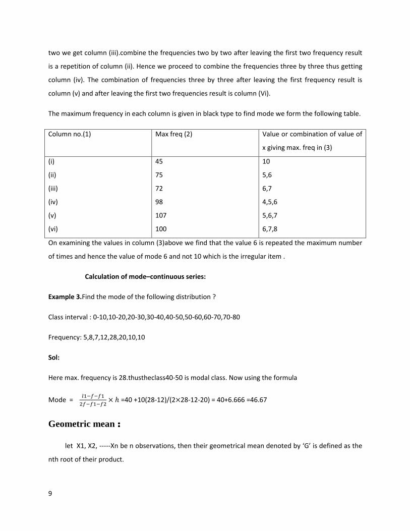
The maximum frequency in each column is given in black type to find mode we form the following table.
Column no.(1) Max freq (2) Value or combination of value of
x giving max. freq in (3)
(i)
(ii)
(iii)
(iv)
(v)
(vi)
45
75
72
98
107
100
10
5,6
6,7
4,5,6
5,6,7
6,7,8
On examining the values in column (3)above we find that the value 6 is repeated the maximum number
of times and hence the value of mode 6 and not 10 which is the irregular item .
Calculation of mode–continuous series:
Example 3.Find the mode of the following distribution ?
Class interval : 0-10,10-20,20-30,30-40,40-50,50-60,60-70,70-80
Frequency: 5,8,7,12,28,20,10,10
Sol:
Here max. frequency is 28.thustheclass40-50 is modal class. Now using the formula
Mode = ����������� × ℎ =40 +10(28-12)/(2×28-12-20) = 40+6.666 =46.67
Geometric mean ::::
let X1, X2, -----Xn be n observations, then their geometrical mean denoted by ‘G’ is defined as the
nth root of their product.
10
i.e, G = (�1, �2, − − −��)��
log G = ∑ � !"#
$
if the value X1 occurs fi times x2 occurs f2 times and so on. Then
Log G = ∑ �� !"
�
Thus the logarithm of the geometric mean of a series of a values is the arithmetic mean of their
logarithms.
Merits:
(i) it is based on all observations.
(ii) it is suitable for the mathematical treatment.
Demerits :
(i) its calculation is rather difficult.
(ii) it is not give the same weight to all the items.
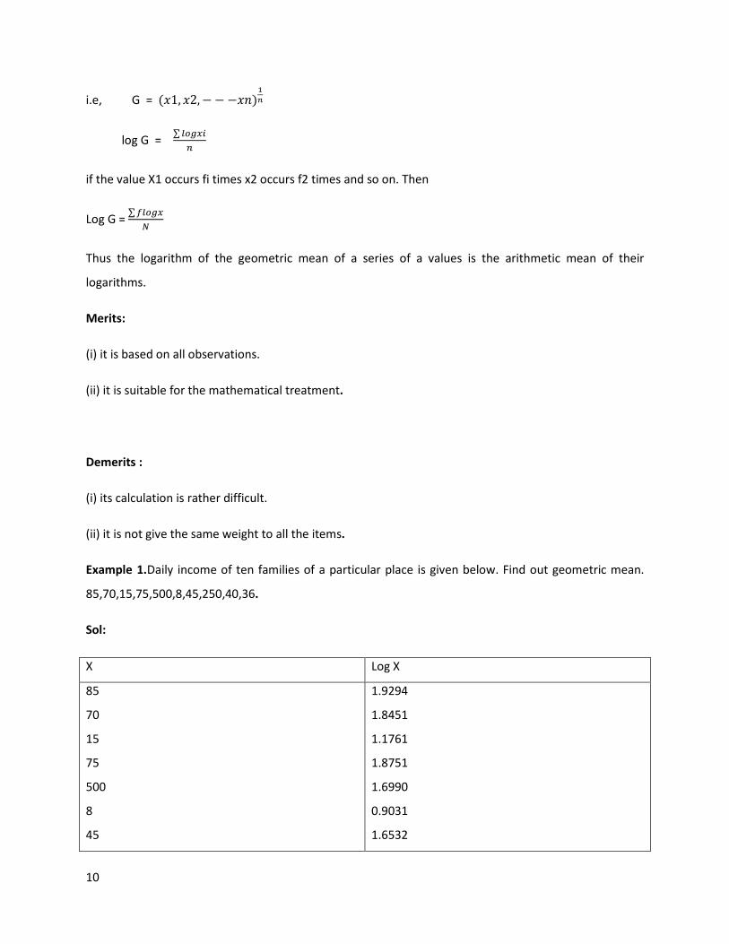
Example 1.Daily income of ten families of a particular place is given below. Find out geometric mean.
85,70,15,75,500,8,45,250,40,36.
Sol:
X Log X
85
70
15
75
500
8
45
1.9294
1.8451
1.1761
1.8751
1.6990
0.9031
1.6532

11
250
40
36
2.3979
1.6021
1.5563
∑ %&'� = 17.6373
G.M = Antilog (17.6373/10) = 58.03
Harmonic mean:
let X1,X2,---,Xn be the n values of a variable X, their harmonic mean denoted by H is defined to
be the reciprocal of the arithmetic mean of their reciprocal.
i.e H = $
∑�(
if the value x1 occurs f1 times, x2 occurs f2times and so on, then
�) =
�� ∑ � �
�
Merits:
(i) it is based on all observations.
(ii) it is suitable for the mathematical treatment.
Demerits :
(i) its calculation is rather difficult.
(ii) it is not give the same weight to all the items.
Example 1.From the following data compute the value of harmonic mean.
Marks: 10 20 25 40 50
No. of students: 20 30 50 15 5

12
Sol:
Marks (x) F f/x
10
20
25
40
50
20
30
50
15
5
2.000
1.500
2.000
0.375
0.100
N =120 ∑ �/� =5.975
H.M =�
∑ �/� =120/5.975 = 20.08
Relation between A.M , G.M and H.M
RELATION:
If a and b are two positive numbers AM≥GM ≥ -.
In any distribution when the original items differ in size , the value of A.M,G.M and H.M. would also
differ and will be in the following order.
AM≥GM ≥ -.
i.e., arithmetic mean is greater than geometric mean is greater than harmonic mean the equality sign
holds only if all the numbers X1,X2---Xn are identical .
proof: let a and b be two positive quantities a≠b. then A.M, and H.M of these quantities are
X =a+b/2; G.M =√1 × 2 ; H.M = 2ab/a+b
as we have to prove A.M>G.M>H.M. Let us first prove that A.M>G.M Or a+b/2 >√1 × 2
=>a+b>2√12
=>a+b-240
=> (√5 − √6)7 >0

13
But square of any real quantity is positive
Hence A.M >G.M (i)
Now let us prove that G.M >H.M
=> √12 > 2ab/a+b
=> a+b/2 >ab/√12
=> a+b/2 > √12
This has already been proved above hence G.M >H.M (ii)
It is clear (i) and (ii) that
A.M > G.M > H.M (iii)
If a and b are equal in that case
AM = G.M. = H.M. (iv)
Thus, 8. ≥ 9.. ≥ -.. proved
Dispersion :
Definition of dispersion :-
Dispersion indicates the measure of the extent to which individual items differ. it indicates lack of
uniformity in the size of items.
According to brooks and dick “dispersion or spread is the degree of the scatter or variation of the
variables about a central value.”
Measures of dispersion –Absolute and Relative :
Absolute measures:
The absolute measures of dispersion can be compared with one another only if the two
belong to the same population and are expressed in the same units like Inches, Kilograms, Rupees etc
.Absolute measures of dispersion do not help us if the series are of different populations or units of

14
measurement. In order to make them comparable a measure ofrelative dispersion is needed by dividing
the absolute measure of dispersion by a measure of central tendency, say mean, median ,mode etc.
Relative measures: the relative measures of dispersion can be found only by calculating .
Range and Coefficient of Range :
Range: Range is the simplest method of studying dispersion. It is defined as the difference between the
value of largest item and the value of the smallest item included in the distribution.
So , Range = L - S
Where L =Largest item
And S = smallest item
The relative measure corresponding to range called the coefficient of range is obtained by applying the
following formula
Coefficient of range = ;<;=<
Merits : It is simplest measure of dispersion .
(ii) It is easily calculated and readily understood.
Demerits : (i) It is very much affected by the fluctuations of sampling.
(ii) Its mathematical treatment is impossible.
Example 1.calculate range and its coefficient for the following data.
Day Price (Rs)
Monday
Tuesday
Wednesday
Thursday
Friday
Satuarday
200
210
208
160
220
250

15
Solution:-Range = L – S
Here L = 250, and S =160
R = 250 -160= 90
Coefficient of range = L – S/L + S =250-160/250+160 = 0.22
Quartile Deviation or Semi inter quartile range:
Quartile deviation and its coefficient:- the half of the inter quartile range is said to be semi inter quartile
range or the quartile deviation =1/2(Q3 - Q1)
and the coefficient of Q.D =
>?@>�>?A>�
=Q3 – Q1/Q3 +Q1
Merits:
(i) It is easy to calculate
(ii)it is simple to understand
Demerits:
(i) It is not based on all observations
(ii) It is not capable of algebraic treatment
Example 2. Find out the value of quartile deviation and its coefficient from the following data
Roll no.: 1 2 3 4 5 6 7
Marks: 20 28 40 12 30 15 50
Sol: First let us arrange the marks in ascending order 12 15 20 28 30 40 50
Q1 = Size of N+1/4TH
Item =size of 7+1/4 =2nd
item

16
Thus Q1 = 15
Q3 = size of 3(N+1/4 )= 6th
item
Q3 = 40
Q.D = Q3 – Q1/2 =40 – 15/2= 12.5
Coefficient of Q.D = Q3 – Q1/Q3 +Q1 = 40 - 15 /40 +15 =25/55 =0.455.
Mean Deviation or Average Deviation:
According to Clark and Schkade “Average deviation is the average amount of scatter
of the items in a distribution from either the mean or the median ,ignoring the signs of the deviations
.The average that is taken of the scatter is an arithmetic mean, which accounts for the fact that this
measure is often called the mean deviation”.
M.D =∑ BCB
� , M.D =∑ �BCB
� (continuous series)
Coefficient of M.D: So the coefficient of mean deviation is defined as DE5F GEHI5JIKF
H5LME KN JOE 5HEP5QE IFHKLHEG
the average may be mean , median or mode.
Example 3. Calculate mean deviation for the following series
X : 10 11 12 13 14
F: 3 12 18 12 3
Sol: calculation of mean deviation
X F IDI FIDI C.F
10
11
12
13
14
3
12
18
12
3
2
1
0
1
2
6
12
0
12
6
3
15
33
45
48
N =48 ∑ �RSR =36

17
M.D =∑ �BCB
�
M.D =36/48 =0.75
Standard deviation or (root mean square deviation):
This concept of S.D was introduced by Karl Pearson in 1832 .the standard deviation measures the
absolute dispersion ,the greater the amount of dispersion or variability the greater the standard
deviation for the greater will be the magnitude of the deviations of the values from their mean. A small
standard deviation means a high degree of uniformity of the observation as well as homogeneity of a
series , a large standard deviation means just the opposite. Hence standard deviation is extremely useful
in judging the representativeness of the mean.
Formula used for calculation OF S.D
T = U∑ �"�� T = U∑ �C
�� − ∑ V�C
� W 2 where d = X- A.
Example4. Calculate the S.D from the following data .
Size of item Frequency
3.5
4.5
5.5
6.5
7.5
8.5
9.5
3
7
22
60
85
32
8
Sol:
Size of item (X) F X -6.5 =d fd fd2
3.5
4.5
5.5
3
7
22
-3
-2
-1
-9
-14
-22
27
28
22

18
6.5
7.5
8.5
9.5
60
85
32
8
0
1
2
3
0
85
61
24
0
85
182
72
N = 217 ∑ �S =128 ∑ �S2 = 362
So standard deviation T = U∑ �C�
� − ∑ V�C� W 2 =
√�X���Y − (128/217)2
T = 1.149.

19
Unit III
------------------------------------------------------------------------------------
SKEWNESS
“When a series is not symmetrical it is said to be asymmetrical or skewed.”
-Croxton and Cowden
Measures of skewness :
1.Absolute measures of skewness:
In a skewed distribution the three measures of central tendency differ. Accordingly skewness
may be worked out in absolute amount with the help of the following formula.
Absolute skewness = X - mode
Absolute skewness = X - median
Absolute skewness = median - mode
(+) and (-) signs will show the direction of skewness and the differenceswill show the extent of
skewness.
2. Relative measures of skewness:
The following are the four important measures of relative skewness ,termed as coefficients of
skewness:
i. The Karl Pearson’s coefficient of skewness.
ii. The Bowley’s coefficient of skewness
iii. The Kelly’s coefficient of skewness .
iv. Measures of skewness based on moments.
The Bowley’s coefficient of skewness:

20
It is based on quartiles Q3 and Q1. In a symmetrical distribution (Q3 -M) –(M- Q1) = 0 But in a
skewed distribution this would not be so.
Thus the second measure of skewness =(Q3 -M) –(M- Q1)
This represents an absolute measure of skewness. For relative measures , we have to divide the
absolute value with the sum of (Q3 -M) and (M- Q1)
Bowley’s coefficient of SK. =13
213
)1()3(
)1()3(
MQQ
QMMQ
QMMQ
−−+=
−+−−−−
This measures is called the quartile measure of skewness and values of the coefficient, thus
obtained vary between ± 1
Example1.Wage distribution of workers in two firms A and B is given below .calculate coefficient of
skewness based on quartiles and point out which distribution is more skewed .
wageRs 55-58 58-61 61-64 64-67 67-70
No. of
works
Firm A
Firm B
12
20
17
22
23
25
18
23
10
8
Sol:
Wages Rs Firm A no. of
workers
cf Firm B no. of
workers
Cf
55-58
58-61
61-64
64-67
67-70
12
17
23
18
10
12
29
52
70
80
20
22
25
13
8
20
42
67
80
88
N =80 N =88
COEFFIIENT OF SKEWNESS =
13
213
MQQ
+−+
FIRM A
Q1 Class = size of the (N/4)th item or (80/4)th item or 20th
item =58-61

21
Q1 = L1 + if
cfN
×−
4= 58 +
(3
17
)1220 ×− = 59.41
Q3 class =size of the (3N/4)th item OR 60TH
Item = 64 -70
Q3 = = L1 + if
cfN
×−
4
3
= 64 + (
318
)5260 ×− = 65.33
Median class = sze of the (N/2)th item or (80/2)th item or 40 th item =61-64
Median = L1 + if
cfN
×−
2= 61+
(3
23
)2940 ×− = 62.43
Coeff. Of SK. =
13
213
MQQ
+−+ =
41.5933.65
43.62241.5933.65
−×−+ =-.02
FIRM B
Q1 Class = size of the (N/4)th item or (88/4)th item or 22nd item =61-64
Q1 = L1 + if
cfN
×−
4= 58 +
(3
22
)2022 ×− = 58.273
Q3 class =size of the (3N/4)th item OR 66TH
Item = 61 -64
Q3 = = L1 + if
cfN
×−
4
3
= 61 + (
325
)4266 ×− = 63.88
Median class = sze of the (N/2)th item or (80/2)th item or 44 th item =61-64
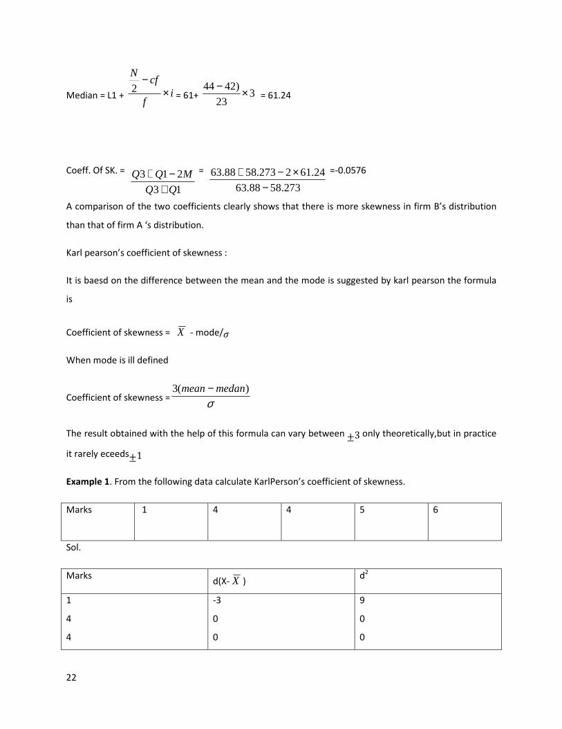
22
Median = L1 + if
cfN
×−
2= 61+ 3
23
)4244 ×− = 61.24
Coeff. Of SK. =
13
213
MQQ
+−+ =
273.5888.63
24.612273.5888.63
−×−+ =-0.0576
A comparison of the two coefficients clearly shows that there is more skewness in firm B’s distribution
than that of firm A ‘s distribution.
Karl pearson’s coefficient of skewness :
It is baesd on the difference between the mean and the mode is suggested by karl pearson the formula
is
Coefficient of skewness = X - mode/T
When mode is ill defined
Coefficient of skewness = σ)(3 medanmean −
The result obtained with the help of this formula can vary between ±3 only theoretically,but in practice
it rarely eceeds±1
Example 1. From the following data calculate KarlPerson’s coefficient of skewness.
Marks 1 4 4 5 6
Sol.
Marks d(X- X )
d2
1
4
4
-3
0
0
9
0
0

23
5
6
1
2
1
4
∑x=20 ∑ d2
= 14
As 4 is repeated: mode =4
T = N
d∑ 2 =
5
14=1.67
Coeff. Of skewness= X - mode/T =4-4/1.67=0/1.67=0
Kelly’s coefficient of skewness.
By using quartiles, bowley’S ignored two extreme quarters of the data in a given problem .
Kelly used deciles and percentiles to cover the entire data and more so to give weightage to the extreme
values.kelly suggested the following formula based on the first and ninth decile or on the 10th
and 90th
percentile. The formula are
Kelly’s coefficient of SK = 19
291
DD
MDD
−−+
=1090
29010
PP
MPP
−−+
This method is not popular in practice and generally Karl Pearson’s methods applied .the
results obtained by all the three formulae will generally lie between +1 and -1. When the distribution is
positively skewed, the coefficient of skewnesss will have plus sign and when it is negatively skewed it
will have negative sign . it should be remembered that the value coefficient will never exceed 1.
Example 1.compute Kelly’s coefficient of skewness.
X 4 8 12 16 20 24 28 32
F 4 9 17 40 53 37 24 16
Sol:
X F Cf
4
8
12
16
4
9
17
40
4
13
30
70

24
20
24
28
32
53
37
24
16
123
160
184
200
N =200
D9 = P90 =size of 90(200+1)/100th
term
=size of 180.9th
term =28
D1 = P10 =size of 10(200+1)/100th
term
=size of 20.1th term =12
Median = size of 200+1/2th term =101.5th
term =20.
Coefficient of sK. = 19
291
DD
MDD
−−+
= 1228
2022812
−×−+
= 0
This series is evenly distributed.
Kurtosis
Kurtosis is a Greek word which means bulginess kurtosis is the degree of peakedness of a
distribution usually taken relative to a normal distribution .In other words; kurtosis measure the
peakedness of a distribution relative to normal distribution .A distribution having a relatively higher
peak than a normal curve is called leptokurtic. Whereas a distribution having a relatively lower peak
than a normal curve which is flat-topped is called platykurtic .The normal curve which is not very peaked
or very flat topped is called mesokurtic.
Measures of kurtosis
Karl Pearson has given beta two (^2) as a measure of kurtosis which is defined as:
^2 = _4_2�a

25
If the value of ^2 =3then the curve is normal or mesokurtic.when the value of ^2 >3 the curve is higher
peaked than the normal which is called leptokurtic and when the value of ^2 <3 the curve is less peaked
than the normal curve ,it is called platykurtic.
Moments :
“moments is a familiar mechanical term for the measure of a force with reference to its
tendency to produce rotation . the strength of this tendency depends, obviously upon the aount of the
force and the distance from the origin of the point at which the force is exerted.”
F.C. Mills
Moments about mean :
If we take the mean of the first power of the deviations we get the first moment about
the mean. The moment of the cubes of the derivation gives us the third moment about the mean and so
on . the moment about mean is called “central moment” and is denoted by the later ′_’ (mu)
The first moment about mean = _1 =N
XX )( −∑
Since sum of deviation of items from arithmetic mean is always zero so _1 would always be zero.
Second moment about mean = _2 == ∑(� X )�
Third moment about mean = _3 == ∑(� X )?�
For frequency distribution
_1 =N
XXf )( −∑
_2 = ∑ �(� X )�
_3 = ∑ �(� X )?�

26
Moments can be extended to higher powers in a similar way but generally first three moments suffice.
Relationship between raw moments and central moments upto 4th
order:
Conversion of moments about an arbitrary origin into moments about mean central and
vice –versa
We have rth about origin and mean
_c == ∑(�# X )d� ; _1′ == ∑(�#e)
�
� − X = (� − a) - ( X − a)
_c = ∑(�#g)d�
Where Xi = (� − a)
d = ax −
using Binomial theorem to _c = ∑(�#g)d� putting r = 1,2,3,4 we get
_1 = _1′ - _1′ =0
_2 = _ 2′ - (_1′ )2
_3 = _ 3′ -3 _1′ _ 2′ +2(_1′ )3
_4 = _ 4′ -4 _1′ _ 3′ +6(_1′ )2 _ 2′ -3(_1′ )
4
Conversely
_ r ′ == ∑(�#e)d� = ∑(�# xx + e)d
�
_ r ′ == ∑( ix ′ g)d�
Where axdandxxiix −=−=′
27
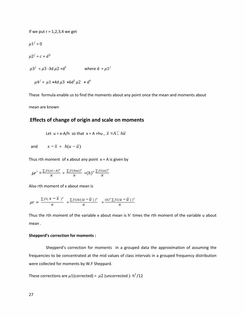
If we put r = 1,2,3,4 we get
_1/ = 0
_2/ = h + S�
_3/ = _3 -3d _2 +d3
where d = _1/
_4/ = _1 +4d _3 +6d2 _2 + d
4
These formula enable us to find the moments about any point once the mean and moments about
mean are known
.Effects of change of origin and scale on moments
Let u = x-A/h so that x = A +hu , uhAx +=
and xx − = )( uuh −
Thus rth moment of x about any point x = A is given by
=′rµ ∑ �#("#i)d� =
∑ �#(jk#)d� =(ℎ)l
∑ �#(k#)d�
Also rth moment of x about mean is
_c = ∑ �#( xx − )d
� = ∑ �#(j#{ uu − } )d
� = (j)d ∑ �#{ uu − } )d
�
Thus the rth moment of the variable x about mean is h’ times the rth moment of the variable u about
mean .
Shepperd’s correction for moments :
Shepperd’s correction for moments in a grouped data the approximation of assuming the
frequencies to be concentrated at the mid values of class intervals in a grouped frequency distribution
were collected for moments by W.F Sheppard.
These corrections are _1(corrected) = _2 (uncorrected )- h2
/12

28
_4(corrected) = _4 (uncorrected)-1/2h2 _2 (o�h&ccphqpS) +7/240h
4
Where h is the width of the class interval. The first and the third moments need no correction.
Now here are some conditions which must be satisfied for the application of Sheppard’s correction.
1. The correction should not be made unless the frequency is at least 1000 otherwise the moments
will be more affected by sampling errors than by grouping errors.
2. The correction is not applicable to J or U shaped distribution or even to the skew for.
3. The observations should be related to a continuous variable.
4. The frequencies should be tapper of to zero in both directions.
So where there will be continuous distribution with above characteristics and where the original
measurement are reasonably precise we may apply the Sheppard’s correction to eliminate the
grouping error.
Beta and gamma measures:
Beta and gamma measures has been devised on the basis of moments as given below:
Beta coefficients 0r Beta measures Gamma coefficients or Gamma measures
rs =tu7t7u
vrs =tu
t7u 7a
r7 =tw
t77
xs =vrs
x 1= r7 -3
=tw
t77 - 3
rs is as a relative measure of skewness in a normal distribution rs will be zero. The greater the value
rs the more skewness will be their in the distribution .but rs can not tell us about the direction (+ or -
) of skewness. This drawback is removed by calculating karl pearson xs which is the square root of rs
i.e vrs .positive tu will have positive skewness and negative tu will give negative skewness of the
distribution r7 is used as a relative measure of kurtosis it measures flatness or peakedness of the curve.
A distribution is normal or mesokurtic when r7 =3 or x7 = 0
A curve is leptokurtic when r7 >3 or x2 is positive and
A curve is platykurtic when r7<3 or xu is negative.

29
UNIT IV
------------------------------------------------------------------------------------
Correlation:
“correlation is an analysis of the co-variation between two or more variables’’
-A.M. Tuttie
‘’the effect of correlation is to reduce the range of uncertainty of one’s prediction’’
-Tippett
Types of correlation:
There are two types of correlation which are discussed as under:
(a) Positive or direct correlation :
if the two variables move in the same direction i.e. with an increase in one
variable, the other variable also increases or with a fall in one variable , the other variable also
falls, the correlation is said to be positive. For example, price and supply are positively related. It
means if price goes up, the supply goes up and vice-versa.
(b) Negative or inverse correlation:
if two variables move in opposite direction i.e. with the increase in one variable
,the other variable falls or with the fall in one variable ,the other variable rises, the correlation is
said to be negative or inverse. For example, the law of demand shows inverse relation between
price and demand .
Methods of correlation
The different methods for studying correlation are ;
(1) Scatter diagram method
(2) Graph method
(3) Karl Pearson ‘s coefficient of correlation
(4) Rank correlation method
(1) SCATTER DIAGRAM METHOD :
When this method used the given data is plotted on a graph paper in
the form of dots I;e for each pair of X and Y value we put a dot and thus obtain
as many points as the observations. By looking on the scatter of the various

30
points we can form an idea as to whether the variables or not .The more plotted
points scatters over a chart ,the less relationship there is between two variables
.the more nearly to the points core to falling line ,.the higher the degree of
relationship.if all the points lie on straight line falling from the lower left hand
corner to the upper right corner .correlation is said to be perfectly positive (i.e r
= +1). On the other hand if the points are lying on the straight line rising from
the upper left hand corner to the lower right hand corner diagram correlation is
said to be perfectly negative (I e; r= - 1). If the plotted point s of all in narrow
band their would be high degree of correlation between the variables –
correlation shall be positive ;if the points show arising tendency from the lower
left hand corner to the upper hand corner .if the point shows a decline tendency
from the upper left hand corner to the lower hand corne
MERTIS :
(i)scattered diagram is avery imple method of studying correlation between two va
riables.
(ii)Scattered diagram also indicates whether the relation is positive or negtive
DEMERITS:
(i)It give only an approximate idea of the relationship
(ii) scattered diagram does not measure the precise extent of correlation
Karl Pearson’s coefficient of correlation or product moment:
Scattered diagram method of correlation merely indicates the direction of
correlation but not its precise magnitude. Karl Pearson has given a quantitative method of calculating
correlation .it is an important and widely Used method of studying correlation. Karl Pearson’s coefficient
of correlation is generally written as ‘r’
Formula :
According to Karl Pearson’s method , the coefficient of correlation is measured as.

31
r = ∑ �y
�z"z{ = ∑ �y
U∑ �×∑ y
Where,
∑ �| = cov(x,y)
r = coefficient of correlation
x = X - X
Y=Y -Y
T� = standard deviation of X series
T} =standard deviation of Y series
N = number of observations.
This formula is applied only to those series where deviations are worked out from actual average of the
series ,it does not apply to those series where deviations are calculated on the basis of assumed mean.
Value of the coefficient of correlation calculated on the basis of this formula may vary between +1 and -
1. However the situations, when r =+1,r =-1, or r =0 are rather rare.generally value of ‘r’varies between
+1 and -1.
1. When r = +1, it means there is perfect positive relation between the variables.
2. When r=-1,it means there is perfect negative relationship between the variables
3. When r = 0,it means that there is no relationship between the variables i.e the variables are
uncorrelated.
Properties of the coefficient of correlation:
Property 1. The coefficient of correlation lies between -1 and +1.symbolically -1≤ c ≤ +1.
Proof: let x and y be deviations of X and Y series from their means and T� and T} be their standard
deviations .Expand the functions.
∑( "z" + {
z{) 2 = ∑( "
z" + {z{ + 2 "{
z"z{) = ∑ "z"+∑ {
z{ + 2 ∑ "{z"z{

32
But ∑ "z" = N
Similarly ∑ {z{ =N also 2 ∑ "{
z"z{ = 2Nr
Hence ∑( "z" + {
z{) 2
=N+N+2Nr =2N +2Nr = 2N(1+r
But ∑( "z" + {
z{) 2
is the sum of squares of real quantities so it can not benegative at the most it can be
zero.
2N(1+r) ≥ 0
Hence r cannot be less than -1at the most it can be -1.
Similarly by expanding ∑( "z" − {
z{)2 it will turn equal to 2N(r-1).
This again cannot be negative ,at the most it can be zero because r can notbe greater than +1, at the
most it can be +1
Hence -1≤ c ≤+1 Hence proved .
Property 2. The coefficient of correlation is independent of change of scale and originof the variable x
and Y.
Proof: By change of origin we mean subtracting some constant from every given value of X and Y and by
changing the scale we mean dividing or multiplying every value of X and Y by some constant.
We know that rxy =2)(2)(
))((
∑ −−−−∑
YYXX
YYXX
Where YandX refer to actul means of X and Y series.
Let us now change the scale and origin deduct a fixed quantity ‘a’ from X and ‘b’ from Y.also divide X
and Y series by a fixed value i and c. after these changes are introduced new values of x obtained from
original X and Y shall be
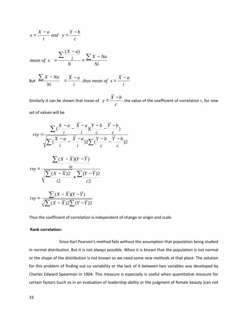
33
c
bYyand
i
aXx
−=−=
Ni
NaX
Ni
aX
xofmean∑∑ −
=
−
=
)(
But i
aXxofmeanthus
i
aX
Ni
NaX −=−=−∑ .
Similarly it can be shown that mean of .c
bXy
−= the value of the coefficient of correlation r, for new
set of values will be
∑∑
∑
−−−−−−
−−−−−−
=2)(2)(
))((
c
bY
c
bY
i
aX
i
aXc
bY
c
bY
i
aX
i
aX
rxy
2
2)(
2
2)(
))((
c
YY
i
XX
ic
YYXX
rxy∑∑
∑
−×
−
−−
=
∑ ∑
∑−−
−−=
2)(2)(
))((
YYXX
YYXXrxy
Thus the coefficient of correlation is independent of change or origin and scale.
Rank correlation:
Since Karl Pearson’s method fails without the assumption that population being studied
in normal distribution. But it is not always possible. When it is known that the population is not normal
or the shape of the distribution is not known so we need some new methods at that place. The solution
for this problem of finding out co variability or the lack of it between two variables was developed by
Charles Edward Spearman in 1904. This measure is especially is useful when quantitative measure for
certain factors (such as in an evaluation of leadership ability or the judgment of female beauty )can not

34
be fixed , but the individual in the group can be arranged in order thereby obtained for each individual a
number indicating his (her) rank in the group. So spearman’s Rank correlation coefficient is defined as :
R = 1 - X ∑ �#
�(��)
Repeated rank correlation:
In some cases it may be found necessary to rank two or more individuals or entries
as equal. In such case it is customary to give each individual an average rank. Thus if two individual are
ranked equal at fifth place they are each given the rank 5+6\2 that is 5.5 while if three are ranked equal
fifth place ,they are given the rank 5 +6 +7/3 =6. In other words these two or more items are to be
ranked equal, the rank assigned for purpose of calculating coefficient of correlation is the average of the
ranks which these individuals would have got had they differed slightly from each other
Where equal ranks are assigned to some entries an adjustment in the above for calculating the rank
coefficient of correlation is made
The adjustment consists of adding 12
3 mm − to the value of ∑D
2.
Where m stands for the number of items four ranks are common. If there are more than one such group
of items will common rank, this value is added as many times the number of such group this formula can
thus be written.
NN
mmmmD
R−
+−+−+−=∑
3
....)12
)3(1
12
)3(12(6
1
Let us now found the limits for the rank correlation coefficient:
Since superman’s rank correlation coefficient is given by
R = 1 - X ∑ �#
�(��)
R is maximum , if ∑ � � is minimum i.e if each of the deviations Diis minimum. But the minimum value
of Di is zero in the particular case xi = yi i.e.if the ranks of the ith individual in the two characteristics
are equal. Hence the maximum value of R is +1 i.e., R≤ 1.

35
R is minimum, if ∑ � � is maximum i.e., if each of the deviation Di is maximum. Which is so if the ranks
of the N individuals in the two characteristics are in the opposite direction?
Case I. suppose N is odd and equal to (2m+1) then the value of D are
D: 2m, 2m-2, 2m-4, …2,0, -2, -4, …, - (2m -2), -2m
∑ � � = 2{(2m)
2 + (2m -2)
2 + ….+4
4 +2
2}
R = 1 - X ∑ �#
�(��) =1 -��(�=�)(���) =-1
caseII. Let N be even and equal to 2m (say) then the value of D are
(2m-1),(2m-3),…1, -1, -3 ,…-(2m-3),-(2m-1)
∑ � � = 2{(2m-1)
2 +(2m-3)
2 +… +1)2}[{(2m)
2+(2m-1)
2+(2m-2)
2+ …2
2 + 1
2}-{(2m)
2+(2m-2)
2+…+4
2+2
2
R = 1 - X ∑ �#
�(��) = 1 -��(���)��(���) =-1
Thus the limits for rank correlation coefficient are given by -1≤ � ≤1
Merits :
1.it is easyto calculate and understand as compared to pearson’s r.
2. This method is employed usefully when the data is given in a qualitative nature like beauty, honesty ,
intelligence etc.
Demerits :
1. This method cannot be employed in a grouped frequency distribution.
2. If the items exceed 30, it is then difficult to find out ranks and their differences
Meaning of Regression :
Definitions:
“regression is the measure of the average relationship between two or more variables in terms of the
original units of the data”. –Morris M. Blair

36
Derivation of two regression lines:
Regression equations through normal equations:
The two main equations generally used in regression analysis are:
(i ) Y on X (ii) X on Y
For Y on X, the equation is Yc = a +bX
For X on Y, the equation is Xc =a +by
A and b are constant values and ‘a’ is called the intercept. In the case of Y on X it is an
estimated value of Y when X is zero and similarly in the case of X on Y, it shows the value of X when Y is
zero. ‘b’ represents the slope of the line, that is change per unit of an independent variable. it is also
known as regression coefficient of Y on X or X on Y as the case may be and also denoted as byx for Y on
x and b xy for X on Y. if ‘b’ is having positive sign before it , regression line will be upward sloping and in
case of negative sign , the line shall be sloping downwards.
Yc or Xc are the values of Y or X computed from the relationship for a given X or Y.
Regression equation of Y on X:
The regression equation of Y on X can be written as Yc = a +bX
We can write at two normal equations as fallows
Given Y = a + bx (i)
Now summate (∑) Eq.(i) ∑Y = Na +b ∑X (ii)
Now multiply the whole equation (ii) by X, we get
∑XY = a∑X + b∑X2 (iii)
Equation (ii) and (iii) are called normal equations
Regression equation of X on Y:
The regression equation of X on Y can be written as Xc = a +bY

37
We can write at two normal equations as fallows
Given X = a + bY (i)
Now summate (∑) Eq.(i) ∑X = Na +b ∑Y (ii)
Now multiply the whole equation (ii) by X, we get
∑XY = a∑Y+ b∑Y2 (iii)
Equation (ii) and (iii) are called normal equations
Regression coefficients and their properties:
The main properties of regression coefficients are as under:
1. Both the regression coefficients bxy and byx cannot be greater than unity that is either both or
less than unity and one of them must be less than unity. In other words the square root of the
product of two regression coefficient must be less than or equal to 1 or -1 or v2�} − 2}� ≤ 1.
2. Both the regression coefficients will have the same sign.
3. Correlation coefficient is the geometric mean between regression coefficients i.e,
r = v6�� × 6�� proof: Regression coefficient of X on Y, 2�} =r
z"z{
Regression coefficient of Y on X , 2}� =rz{z"
Therefore product of the two regression coefficients r z"z{ × r z{
z" =c�
Therefore c� = 2�} × 2}�
Or r = ± v2�} × 2}� Here +veor –ve sign is taken before the radical sign according as 2�} and 2}�
are both +ve or –ve.
4.Regression coefficients are independent of change of origin but not scale .
Proof: As shown in property of correlation coefficient .

38
Principal of least square :
In practice, the method of least squares is widely used. This is the mathematical
method with the help of which a trend line is fitted to the data in such a way that the two
conditions are satisfied i.e.
1. ∑(Y- Yc) = 0.
It means the sum of deviation of the actual of Y and the computed values of Y is zero .
2. ∑(Y- Yc)2 is minimum .
It means the sum of the squares of deviations of the actual and computed values is
minimum from this line. It is because of this reason that we call this method as ‘method of
least squares’ the line which we get by this method is known as the ‘line of best fit.
The straight line trend is shown by the equation
Yc = a +bX (i)
Yc is the trend values to distinguish from the actual Y values, a is the intercept of the
values of the Y variable when X =0, b is the slope of the line , X refers to time.
Determine the constants ‘a’ and ‘b’:
For determining the values of the constant a and b, the two normal
equations are to be solved simultaneously:
Sum up equation (i), we get ∑Y = Na + b∑X (ii)
Now multiply equation(ii) by X we get ∑XY =a∑X + b∑x2
(iii)
N denotes the number of years. the equation (ii) is the summation of equation (i) where as
equation (iii) is the summation of X multiplied to equation (ii)
Variable X can be measured from any point of time in origin such as first year. The
calculation becomes simple when the mid point in time is taken as the origin because in
that case the negative values in the first half of the series balance out the positive values in
the second half so that ∑X = 0as the deviaXons are taken from the mean As ∑X = 0the
equation(ii) and (iii) can be written as
∑Y = Na
1 = ∑ y� = Y
And ∑XY = b∑X2
Or b = ∑ �y∑ �

39
The constant ‘a’ gives the arithmetic mean of Y nd the constant ‘b’ shows the rate of
change.
Merits :
1. Since it is a mathematical method of measuring trend so there can be no possibility of
subjectiveness.
2. The trend equation can be used to estimate or predict the values of the variable for any
period t in future and the forecasted values are also reliable.
Demerits:
1. It is difficult to determine the type of the trend curve to be fitted i.e., whether to fit a
linear or a parabolic trend or some other complicated trend curve.
2. This method is tedious and time consuming as it requires more calculations as
compared with other methods.
Example 1. Fit a straight line to the following data?
Solution:-
Year (X) Production (Y) X X2 XY Yc
1975
1976
1977
1978
1979
1980
1981
1982
1983
1984
1985
61
66
72
76
82
90
96
100
103
110
114
-5
-4
-3
-2
-1
0
1
2
3
4
5
25
16
9
4
1
0
1
4
9
16
25
-305
-264
-216
-152
-82
0
96
200
309
440
570
61.09
66.50
71.92
77.34
82.76
88.16
93.6
99.02
104.44
109.86
115.28
∑Y = 970 ∑X =0 ∑x2 = 110 ∑XY =596
∑Y = Na + b∑X

40
∑XY =a∑X + b∑x2
970 = 11a
A = 970/11 = 88.18
596 = 110b
B = 596/110 = 5.42
Yc = a+ bX
Yc = 88.18 +5.42(X)
Y1975 = 88.18+5.42(-5) = 61.09
Y1976 = 88.18 +5.42(-4) =66.50 and so on.
Fitting of second degree parabola:
The simplest non linear trend is the second degree parabola which can be written in the
form
Yc=a+bx+cX2
The name second degree show that the highest power of x variable is 2 in the
equation .there are three unknown constants a, b and c in the equation where a is the
intercept y, b is the slope of the curve at the origin and c is the rate of change in the slope
the value of a, b, and c can be determined by solving the following three normal equation
simultaneously by the method at least squares:
∑ ∑ ∑++= 2XCXbNaY (i)
∑ ∑ ∑∑ ++= 32 XCXbXaXY (ii)
∑ ∑ ∑∑ ++= 4322 XCXbXaYX (iii)
The above equations are further simplified when time origin is taken between two
middle years where ∑X would be zero .the the equaXons rae reduced to.

41
∑Y = Na + C∑X2
(iv)
∑XY = b∑X2 (v)
∑X2Y = a ∑X
2 + c∑X
4 (vi)
Solving equation (iv) and (v). we obtain the values of a and c and the value of b can directly
be obtained from equation (v)
a =∑ y� ∑ �
�
b = ∑ �y∑ �
c =� ∑ �y∑ � ∑ y� ∑ � (∑ �)�
Example 2. The following are data on the production,(in ‘000 units )of a commodity fro the
taear 1990-1996
Year 1990 1991 1992 1993 1994 1995 1996
Production
in(’000
units)
6 7 5 4 6 7 5
Fit the second degree parabola of the above data.
Sol:
To determine the values of a,b and c we solve the following normal equations
∑ ∑ ∑++= 2XCXbNaY
∑ ∑ ∑∑ ++= 32 XCXbXaXY
∑ ∑ ∑∑ ++= 4322 XCXbXaYX
Year (X) Production
(Y)
X X2 X
3 X
4 XY X
2Y

42
1990
1991
1992
1993
1994
1995
1996
6
7
5
4
6
7
5
-3
-2
-1
0
1
2
3
9
4
1
0
1
4
9
-27
-8
1
0
1
8
27
81
16
1
0
1
16
81
-18
-14
-5
0
6
14
15
54
28
5
0
6
28
45
+
∑Y = 40 ∑X = 0 ∑x2
=28 ∑x3
= 0 ∑x4
=196 ∑XY =-2 ∑X2Y =
166
Substituting the values obtained from the table in the normal equation ,we get
40 =7a +28c
-2 = 28b
166 = 28a +196c
Solving them we get a = 5.429 ,b = -0.071 c = o.71
The equation of the parabola is Y = a+bX+cX2
Substituting the values of unknowns we get
Y = 5.429 -0.071X +0.71X2 .
Govt. Degree College Boys Anantnag
Department of STATISTICS
Faculty member: Mr waqar younus
Head of the department : Dr Aijaz Ahmad Hakak

43