1

Unit 7

Sources of magnetic field

7.1 Introduction

7.2 Oersted’s experiment

7.3 Biot and Savart’s law

7.4 Magnetic flux

7.5 Ampère’s law

7.6 Magnetism in matter

7.7 Problems

Objectives

• Use the Biot and Savart’s law to calculate the magnetic field created in the center of a circular loop flowed by a current

• Define the flux of a magnetic field.

• Use Ampère’s law to calculate the magnetic field created by straight conductors, circular loops and coils.

• Explain the ferromagnetism by mean of theory of Weiss do-mains. Know the hysteresis curve.

7.1 Introduction

In unit 6 we have studied the forces produced by magnetic fields on mov-ing charges and electric currents. In this unit, we are going to study how create such magnetic fields, and we’ll see that their origin are the moving charges and the electric currents.

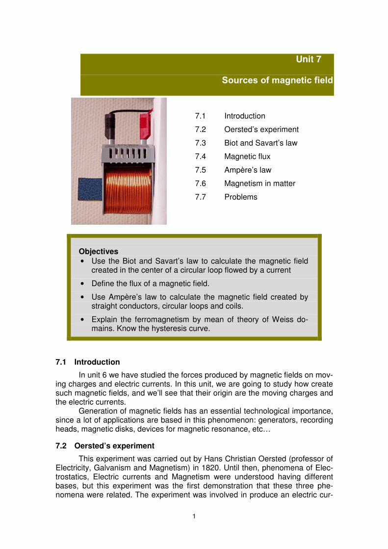
Generation of magnetic fields has an essential technological importance, since a lot of applications are based in this phenomenon: generators, recording heads, magnetic disks, devices for magnetic resonance, etc…

7.2 Oersted’s experiment

This experiment was carried out by Hans Christian Oersted (professor of Electricity, Galvanism and Magnetism) in 1820. Until then, phenomena of Elec-trostatics, Electric currents and Magnetism were understood having different bases, but this experiment was the first demonstration that these three phe-nomena were related. The experiment was involved in produce an electric cur-

2

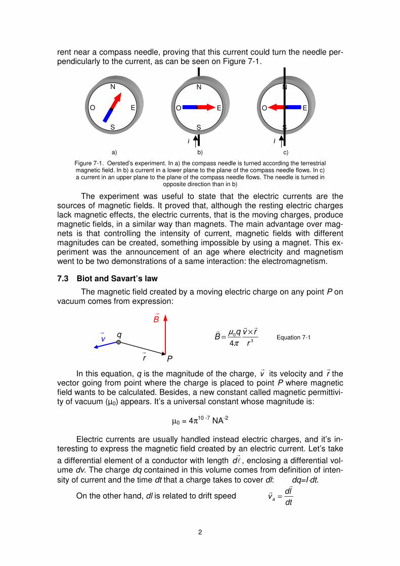
rent near a compass needle, proving that this current could turn the needle per-pendicularly to the current, as can be seen on Figure 7-1.

N

S

E O

I

N

S

E O

I

N

S

E O

a) b) c)

Figure 7-1. Oersted’s experiment. In a) the compass needle is turned according the terrestrial magnetic field. In b) a current in a lower plane to the plane of the compass needle flows. In c) a current in an upper plane to the plane of the compass needle flows. The needle is turned in

opposite direction than in b)

The experiment was useful to state that the electric currents are the sources of magnetic fields. It proved that, although the resting electric charges lack magnetic effects, the electric currents, that is the moving charges, produce magnetic fields, in a similar way than magnets. The main advantage over mag-nets is that controlling the intensity of current, magnetic fields with different magnitudes can be created, something impossible by using a magnet. This ex-periment was the announcement of an age where electricity and magnetism went to be two demonstrations of a same interaction: the electromagnetism.

7.3 Biot and Savart’s law

The magnetic field created by a moving electric charge on any point P on vacuum comes from expression:

r

v

r r P

r

B

q

3

0

4 r

rvqB

rrr ×

=π

µ Equation 7-1

In this equation, q is the magnitude of the charge, vr

its velocity and rr

the vector going from point where the charge is placed to point P where magnetic field wants to be calculated. Besides, a new constant called magnetic permittivi-ty of vacuum (µ0) appears. It’s a universal constant whose magnitude is:

µ0 = 4π10 -7 NA-2

Electric currents are usually handled instead electric charges, and it’s in-teresting to express the magnetic field created by an electric current. Let’s take

a differential element of a conductor with length lr

d , enclosing a differential vol-ume dv. The charge dq contained in this volume comes from definition of inten-

sity of current and the time dt that a charge takes to cover dl: dq=I⋅dt.

On the other hand, dl is related to drift speed dt

ldva

rr

=

3

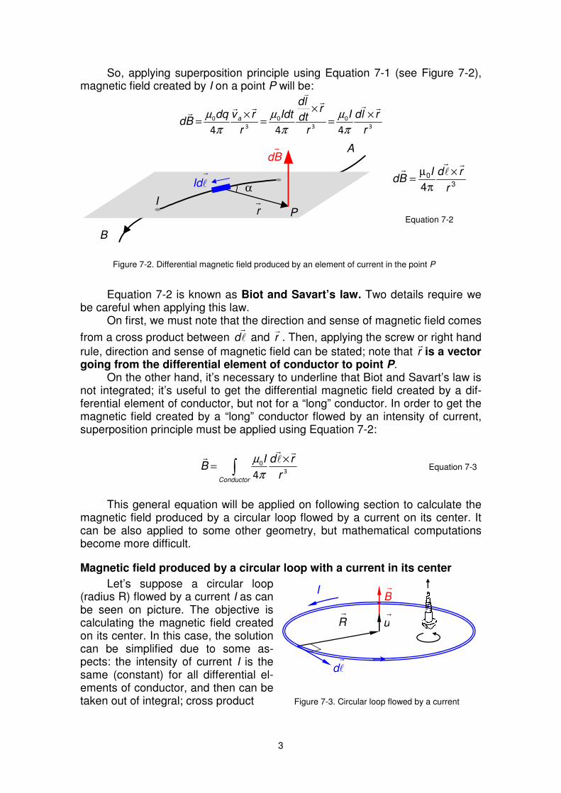
So, applying superposition principle using Equation 7-1 (see Figure 7-2), magnetic field created by I on a point P will be:

3

0

3

0

3

0

444 r

rldI

r

rdt

ldIdt

r

rvdqBd a

rrrv

rrr ×

=

×

=×

=π

µ

π

µ

π

µ

Equation 7-2 is known as Biot and Savart’s law. Two details require we be careful when applying this law.

On first, we must note that the direction and sense of magnetic field comes

from a cross product between lr

d and rr

. Then, applying the screw or right hand

rule, direction and sense of magnetic field can be stated; note that rr

is a vector going from the differential element of conductor to point P.

On the other hand, it’s necessary to underline that Biot and Savart’s law is not integrated; it’s useful to get the differential magnetic field created by a dif-ferential element of conductor, but not for a “long” conductor. In order to get the magnetic field created by a “long” conductor flowed by an intensity of current, superposition principle must be applied using Equation 7-2:

∫×

=Conductor

r

rdIB

3

0

4

rlr

r

π

µ Equation 7-3

This general equation will be applied on following section to calculate the

magnetic field produced by a circular loop flowed by a current on its center. It can be also applied to some other geometry, but mathematical computations become more difficult.

Magnetic field produced by a circular loop with a current in its center

Let’s suppose a circular loop (radius R) flowed by a current I as can be seen on picture. The objective is calculating the magnetic field created on its center. In this case, the solution can be simplified due to some as-pects: the intensity of current I is the same (constant) for all differential el-ements of conductor, and then can be taken out of integral; cross product Figure 7-3. Circular loop flowed by a current

r

Idl

r

r P

r

dB

α

I

B

A

30

4 r

rdIBd

rlr

r ×

π

µ=

Equation 7-2

Figure 7-2. Differential magnetic field produced by an element of current in the point P

I

r dl

r B

r R

r u

4

Rdr

lr

× for all differential elements of conductor point in the same direction and

so, we can integrate only the modulus of magnetic field ( lr

d is the tangent vec-tor to circumference on each point); the distance between each differential ele-ment of conductor and the center of loop is also a constant. For any differential

element udlRRdrdrr

lrr

lr

=×=× , where ur

is the unit vector perpendicular to

plane of loop. Note that sense of ur

is also given by applying the screw rule to the sense of intensity of current. Applying Equation 7-3:

uR

IuR

R

Iu

R

RdI

R

RdIB

RR

center

rrrlr

lr

r

22

444

0

2

0

2

0

3

0

2

0

3

0 µπ

π

µ

π

µ

π

µππ

===×

= ∫∫

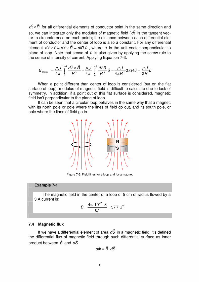
When a point different than center of loop is considered (but on the flat surface of loop), modulus of magnetic field is difficult to calculate due to lack of symmetry. In addition, if a point out of this flat surface is considered, magnetic field isn’t perpendicular to the plane of loop.

It can be seen that a circular loop behaves in the same way that a magnet, with its north pole or pole where the lines of field go out, and its south pole, or pole where the lines of field go in.

S

N

Figure 7-3. Field lines for a loop and for a magnet

Example 7-1

The magnetic field in the center of a loop of 5 cm of radius flowed by a 3 A current is:

T7,37

1,0

3104 7

µ=⋅⋅π

=−

B

7.4 Magnetic flux

If we have a differential element of area Sdr

in a magnetic field, it’s defined the differential flux of magnetic field through such differential surface as inner

product between Br

and Sdr

SdBdrr

⋅=Φ

5

Magnetic flux is measured in Tm2, in I.S. This unit is called weber (Wb). If we consider not a differential area, but any area S, magnetic flux of magnetic field through area S is the addition (integral) of all the differential fluxes:

∫ ⋅=Φ

S

SdBrr

Equation 7-4

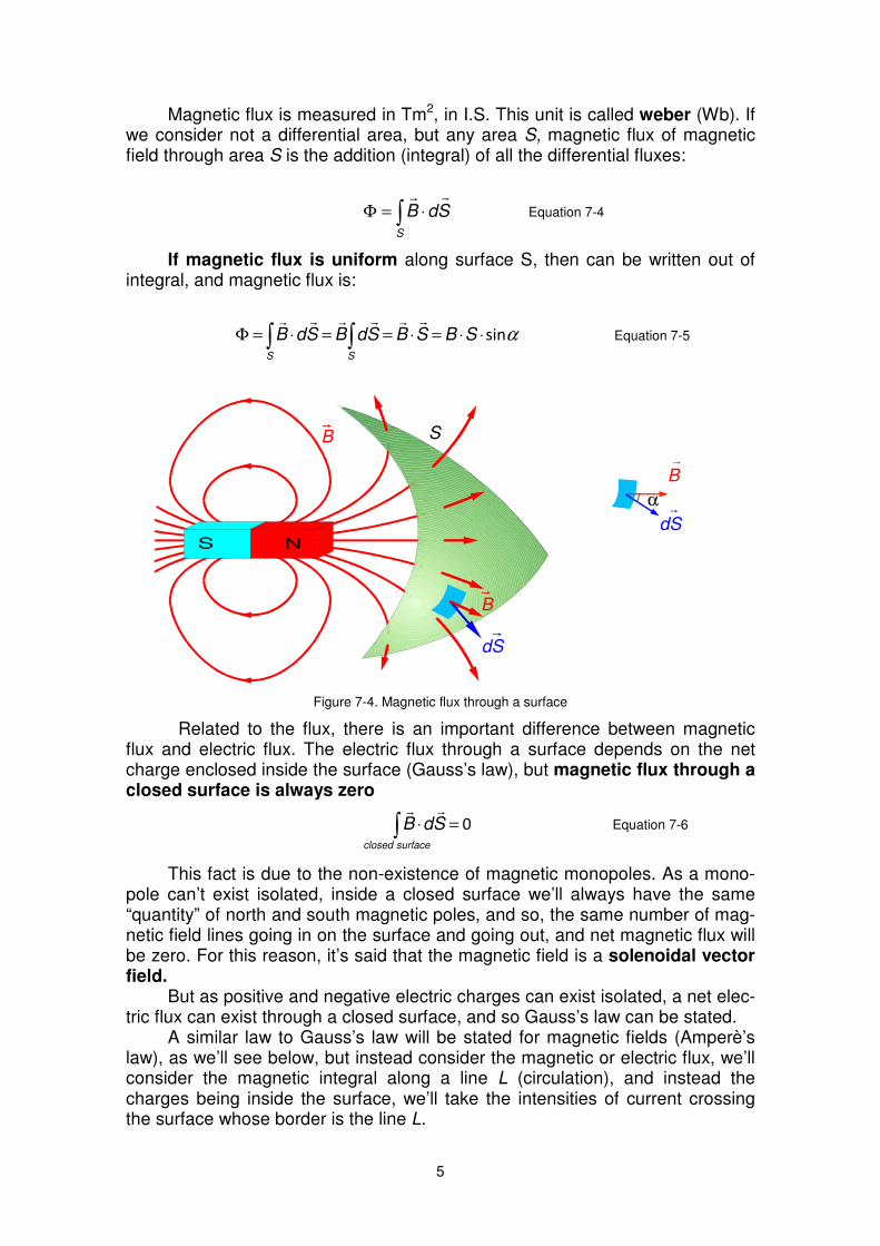
If magnetic flux is uniform along surface S, then can be written out of integral, and magnetic flux is:

αsin⋅⋅=⋅==⋅=Φ ∫∫ SBSBSdBSdBSS

rrrrrr

Equation 7-5

Br

dSr

Br

S

r dS

r B

α

Figure 7-4. Magnetic flux through a surface

Related to the flux, there is an important difference between magnetic flux and electric flux. The electric flux through a surface depends on the net charge enclosed inside the surface (Gauss’s law), but magnetic flux through a closed surface is always zero

0=⋅∫surfaceclosed

SdBrr

Equation 7-6

This fact is due to the non-existence of magnetic monopoles. As a mono-pole can’t exist isolated, inside a closed surface we’ll always have the same “quantity” of north and south magnetic poles, and so, the same number of mag-netic field lines going in on the surface and going out, and net magnetic flux will be zero. For this reason, it’s said that the magnetic field is a solenoidal vector field.

But as positive and negative electric charges can exist isolated, a net elec-tric flux can exist through a closed surface, and so Gauss’s law can be stated.

A similar law to Gauss’s law will be stated for magnetic fields (Amperè’s law), as we’ll see below, but instead consider the magnetic or electric flux, we’ll consider the magnetic integral along a line L (circulation), and instead the charges being inside the surface, we’ll take the intensities of current crossing the surface whose border is the line L.

6

r

E

S

r

B

S

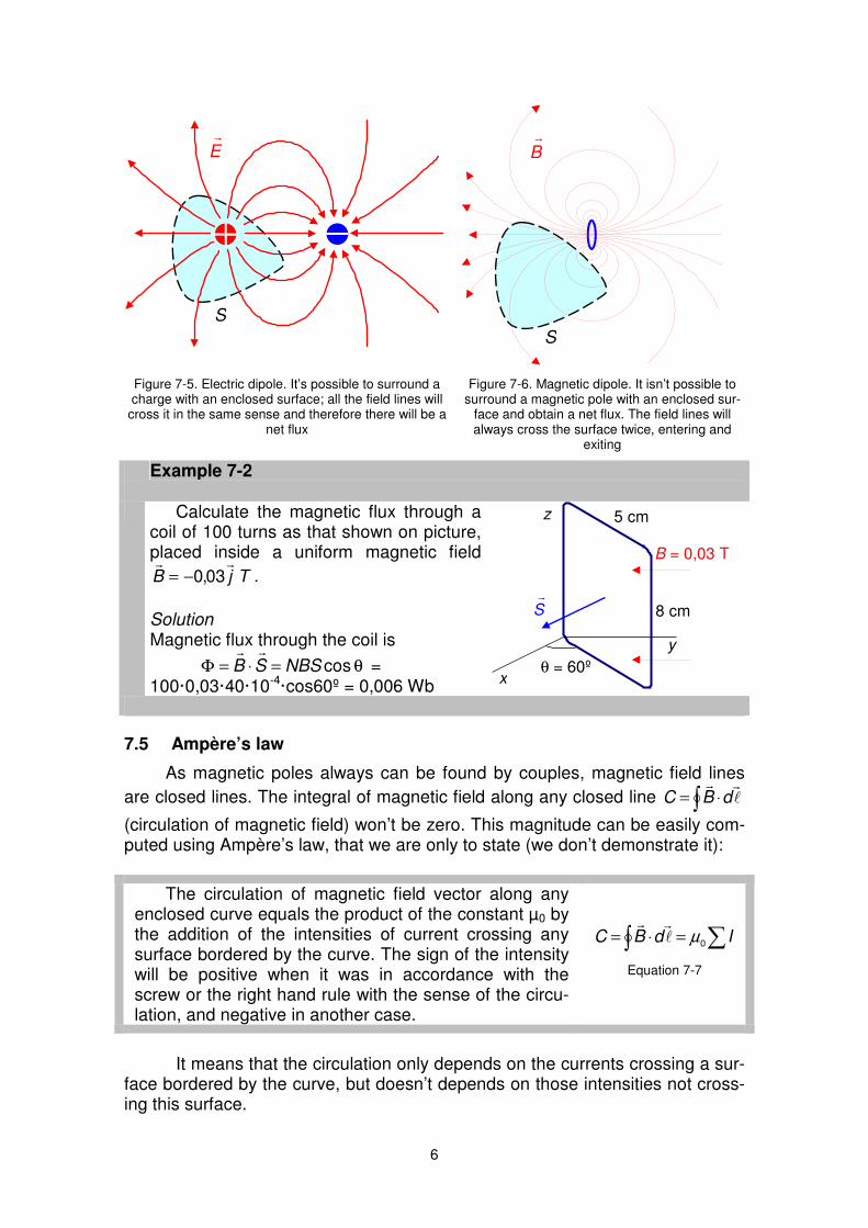
Figure 7-5. Electric dipole. It’s possible to surround a charge with an enclosed surface; all the field lines will

cross it in the same sense and therefore there will be a net flux

Figure 7-6. Magnetic dipole. It isn’t possible to surround a magnetic pole with an enclosed sur-

face and obtain a net flux. The field lines will always cross the surface twice, entering and

exiting

Example 7-2

Calculate the magnetic flux through a coil of 100 turns as that shown on picture, placed inside a uniform magnetic field

TjBrr

03,0−= .

Solution Magnetic flux through the coil is

θ=⋅=Φ cosNBSSBrr

= 100·0,03·40·10-4·cos60º = 0,006 Wb

θ = 60º

8 cm

5 cm

y

x

z

B = 0,03 T

r

S

7.5 Ampère’s law

As magnetic poles always can be found by couples, magnetic field lines

are closed lines. The integral of magnetic field along any closed line ∫ ⋅= lrr

dBC

(circulation of magnetic field) won’t be zero. This magnitude can be easily com-puted using Ampère’s law, that we are only to state (we don’t demonstrate it):

The circulation of magnetic field vector along any enclosed curve equals the product of the constant µ0 by the addition of the intensities of current crossing any surface bordered by the curve. The sign of the intensity will be positive when it was in accordance with the screw or the right hand rule with the sense of the circu-lation, and negative in another case.

∫ ∑=⋅= IdBC0

µlrr

Equation 7-7

It means that the circulation only depends on the currents crossing a sur-

face bordered by the curve, but doesn’t depends on those intensities not cross-ing this surface.

7

I

r

B

r

dl

I1I2

I3

I4 r

B r

dl

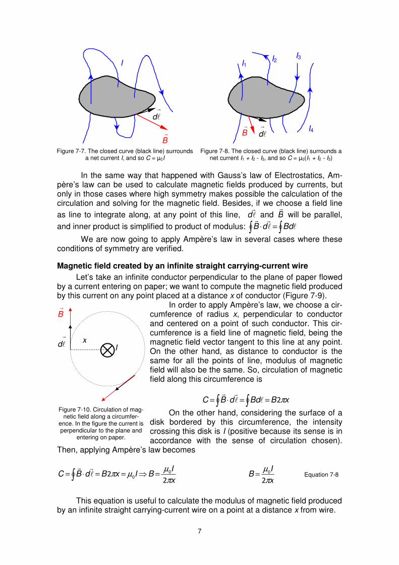
Figure 7-7. The closed curve (black line) surrounds a net current I, and so C = µ0I

Figure 7-8. The closed curve (black line) surrounds a net current I1 + I2 - I3, and so C = µ0(I1 + I2 - I3)

In the same way that happened with Gauss’s law of Electrostatics, Am-

père’s law can be used to calculate magnetic fields produced by currents, but only in those cases where high symmetry makes possible the calculation of the circulation and solving for the magnetic field. Besides, if we choose a field line

as line to integrate along, at any point of this line, lr

d and Br

will be parallel,

and inner product is simplified to product of modulus: ∫∫ =⋅ llrr

BddB

We are now going to apply Ampère’s law in several cases where these conditions of symmetry are verified.

Magnetic field created by an infinite straight carrying-current wire

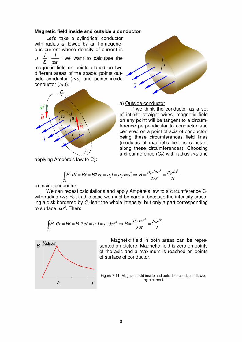
Let’s take an infinite conductor perpendicular to the plane of paper flowed by a current entering on paper; we want to compute the magnetic field produced by this current on any point placed at a distance x of conductor (Figure 7-9).

In order to apply Ampère’s law, we choose a cir-cumference of radius x, perpendicular to conductor and centered on a point of such conductor. This cir-cumference is a field line of magnetic field, being the magnetic field vector tangent to this line at any point. On the other hand, as distance to conductor is the same for all the points of line, modulus of magnetic field will also be the same. So, circulation of magnetic field along this circumference is

xBBddBC π2==⋅= ∫∫ llrr

On the other hand, considering the surface of a disk bordered by this circumference, the intensity crossing this disk is I (positive because its sense is in accordance with the sense of circulation chosen).

Then, applying Ampère’s law becomes

x

IBIxBdBC

π

µµπ

22 0

0 =⇒==⋅= ∫ lrr

x

IB

π

µ

2

0= Equation 7-8

This equation is useful to calculate the modulus of magnetic field produced

by an infinite straight carrying-current wire on a point at a distance x from wire.

xI

r

B

r

dl

Figure 7-10. Circulation of mag-netic field along a circumfer-

ence. In the figure the current is perpendicular to the plane and

entering on paper.

8

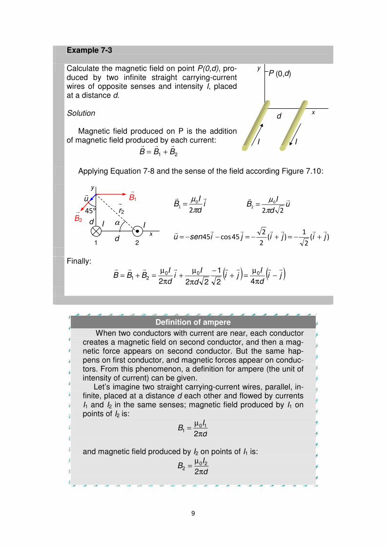
Magnetic field inside and outside a conductor

Let’s take a cylindrical conductor with radius a flowed by an homogene-ous current whose density of current is

2a

I

S

IJ

π== ; we want to calculate the

magnetic field on points placed on two different areas of the space: points out-side conductor (r>a) and points inside conductor (r<a).

a) Outside conductor

If we think the conductor as a set of infinite straight wires, magnetic field on any point will be tangent to a circum-ference perpendicular to conductor and centered on a point of axis of conductor, being these circumferences field lines (modulus of magnetic field is constant along these circumferences). Choosing a circumference (C2) with radius r>a and

applying Ampère’s law to C2:

r

Ja

r

aJBaJIrBBdB

C22

2

2

0

2

02

00

2

µ

π

πµπµµπ ==⇒====⋅∫ ll

rr

b) Inside conductor We can repeat calculations and apply Ampère’s law to a circumference C1

with radius r<a. But in this case we must be careful because the intensity cross-ing a disk bordered by C1 isn’t the whole intensity, but only a part corresponding

to surface Jπr2. Then:

222 0

2

02

00

1

Jr

r

rJBrJIrBBdB

C

µ

π

πµπµµπ ==⇒==⋅==⋅∫ ll

rr

Magnetic field in both areas can be repre-

sented on picture. Magnetic field is zero on points of the axis and a maximum is reached on points of surface of conductor.

Figure 7-11. Magnetic field inside and outside a conductor flowed by a current

a

Jr

a

Jr r

r

r

r

rdl

B

B

C2

C1

r

B

a

½µ0Ja

9

Example 7-3

Calculate the magnetic field on point P(0,d), pro-duced by two infinite straight carrying-current wires of opposite senses and intensity I, placed at a distance d. Solution

Magnetic field produced on P is the addition of magnetic field produced by each current:

21 BBBrrr

+=

P (0,d)

I I

x

y

d

Applying Equation 7-8 and the sense of the field according Figure 7.10:

I I x

y

d 1 2

r

B1

r

B2

r

r2

α

°45

ur

d

id

IB

rr

π

µ

2

0

1 =

ud

IB

rr

22

0

2π

µ=

)(2

1)(

2

245cos45 jijijisenu

rrrrrrr+−=+−=−−=

Finally:

( ) ( )jid

Iji

d

Ii

d

IBBB

rrrrrrrr

−π

µ=+

−

π

µ+

π

µ=+=

42

1

222000

21

Definition of ampere

When two conductors with current are near, each conductor creates a magnetic field on second conductor, and then a mag-netic force appears on second conductor. But the same hap-pens on first conductor, and magnetic forces appear on conduc-tors. From this phenomenon, a definition for ampere (the unit of intensity of current) can be given. Let’s imagine two straight carrying-current wires, parallel, in-finite, placed at a distance d each other and flowed by currents I1 and I2 in the same senses; magnetic field produced by I1 on points of I2 is:

d

IB

π

µ=

210

1

and magnetic field produced by I2 on points of I1 is:

d

IB

π

µ=

220

2

10

In both cases, magnetic field is perpendicular to the plane made up by both currents. As a consequence, both forces will appear on I1 and I2. These forc-

es, for a length l of conductor, will be:

)(2

2102121 u

d

IIBIF

rl

r

lrr

π

µ=×=

)(2

2101212 u

d

IIBIF

rl

r

lrr

−π

µ=×=

d

I2

I1 rB2

rB1

rF21

rF12

r

l

Both forces are equal in modulus and of opposite senses. Then, both conductors attract themselves. If currents would have op-posite senses, then the force between them would be rejecting. So, a definition for ampere is: One ampere is the intensity of current having two infinite, straight and parallel conductors when, placed at a distance of

one meter, a force of 2⋅10 -7 N by meter of length appears be-tween themselves.

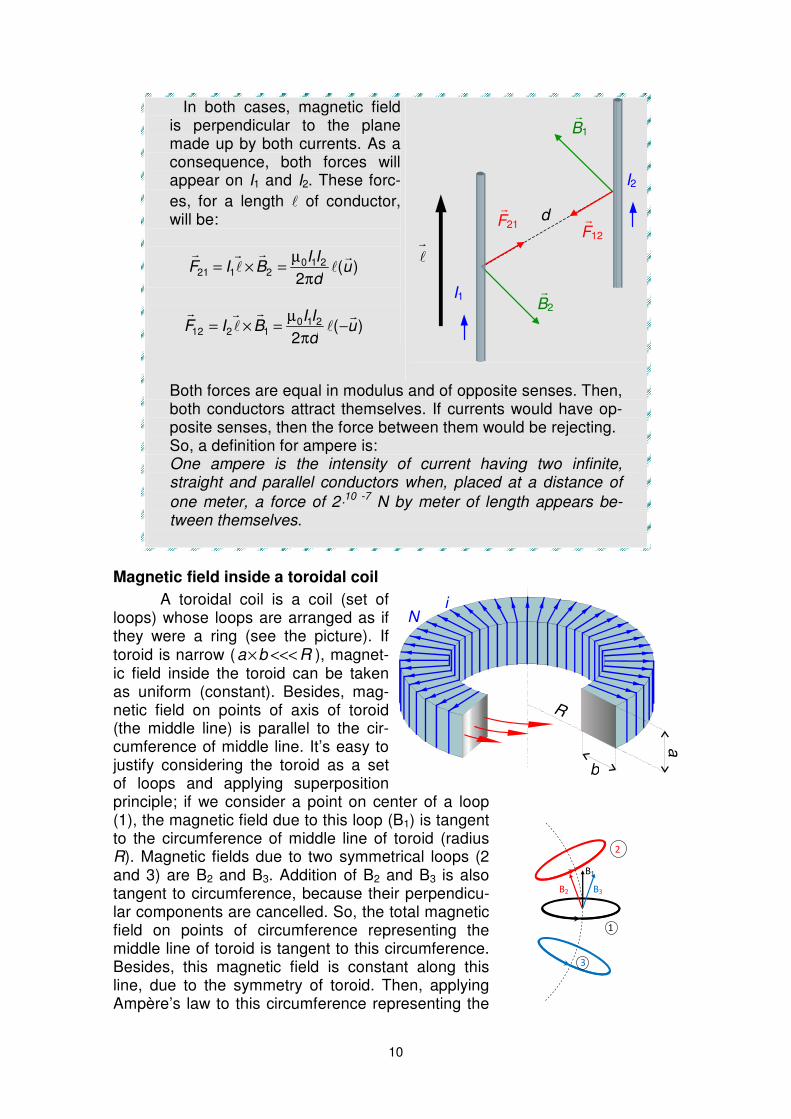
Magnetic field inside a toroidal coil

A toroidal coil is a coil (set of loops) whose loops are arranged as if they were a ring (see the picture). If toroid is narrow ( Rba <<<× ), magnet-ic field inside the toroid can be taken as uniform (constant). Besides, mag-netic field on points of axis of toroid (the middle line) is parallel to the cir-cumference of middle line. It’s easy to justify considering the toroid as a set of loops and applying superposition principle; if we consider a point on center of a loop (1), the magnetic field due to this loop (B1) is tangent to the circumference of middle line of toroid (radius R). Magnetic fields due to two symmetrical loops (2 and 3) are B2 and B3. Addition of B2 and B3 is also tangent to circumference, because their perpendicu-lar components are cancelled. So, the total magnetic field on points of circumference representing the middle line of toroid is tangent to this circumference. Besides, this magnetic field is constant along this line, due to the symmetry of toroid. Then, applying Ampère’s law to this circumference representing the

a

R

b

iN

1

2

3

B1

B3 B2

11

middle line of toroid: RBdBCC

π2=⋅= ∫ lrr

and considering the disk bordered by this circumference, this disk is crossed once by each loop in the same sense, and then the total current crossing the

disk will be NII =∑

Then, from Ampère’s law, we can get the magnetic field on points inside the toroid:

R

NIBNIRB

π

µµπ

22 0

0=⇒= Equation 7-9

The sense of magnetic field points according screw or right hand rule for intensity of current.

On points outside the toroid, if we consider a circumference (radius r) passing by this point (both for r<R or r>R), the intensity of current crossing the disk bordered by this circumference is zero, and magnetic field on points of such circumferences is zero.

Magnetic field inside a straight carrying-current coil

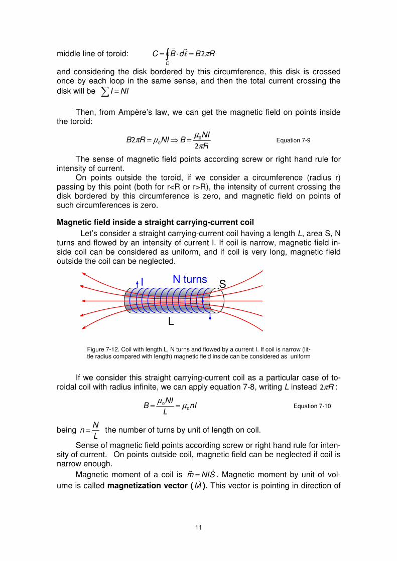
Let’s consider a straight carrying-current coil having a length L, area S, N turns and flowed by an intensity of current I. If coil is narrow, magnetic field in-side coil can be considered as uniform, and if coil is very long, magnetic field outside the coil can be neglected.

I N turns

L

S

Figure 7-12. Coil with length L, N turns and flowed by a current I. If coil is narrow (lit-tle radius compared with length) magnetic field inside can be considered as uniform

If we consider this straight carrying-current coil as a particular case of to-roidal coil with radius infinite, we can apply equation 7-8, writing L instead Rπ2 :

nIL

NIB

0

0 µµ

==

Equation 7-10

being L

Nn =

the number of turns by unit of length on coil.

Sense of magnetic field points according screw or right hand rule for inten-sity of current. On points outside coil, magnetic field can be neglected if coil is narrow enough.

Magnetic moment of a coil is SNImrr

= . Magnetic moment by unit of vol-

ume is called magnetization vector (Mr

). This vector is pointing in direction of

12

axis of coil and its sense is given by the screw or right hand rule for intensity of

current on coil. Its modulus is nIL

NI

LS

NIS

V

mM ==

⋅==

So, magnetic field inside a coil and magnetization of a coil are related through equation

MBrr

0µ= Equation 7-11

Example 7-4

Calculate the magnetic flux through a coil of length 25 cm, radius 1 cm and 4000 turns; a 4 A current flows along coil. Solution As length of coil is 25 times its radius, magnetic field inside coil can be taken as uniform:

L

NIB 0µ

=

And magnetic flux crossing the coil will be N times the magnetic flux cross-ing a loop:

Wb101,025,0

01,04400010422722

0

2

0 =⋅⋅⋅

====Φ− πππµµ

L

rIN

L

ISNNBS

7.6 Magnetism in matter. Magnetization. Ferromagnetism. Hysteresis curve.

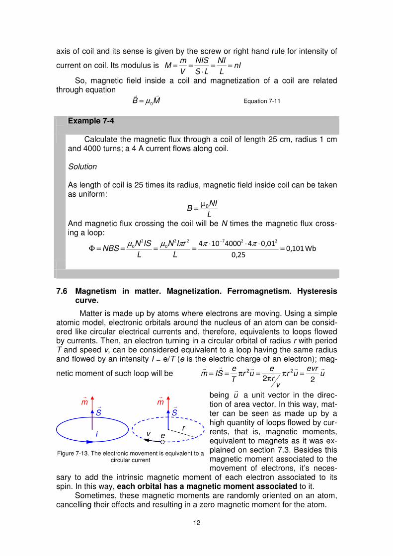
Matter is made up by atoms where electrons are moving. Using a simple atomic model, electronic orbitals around the nucleus of an atom can be consid-ered like circular electrical currents and, therefore, equivalents to loops flowed by currents. Then, an electron turning in a circular orbital of radius r with period T and speed v, can be considered equivalent to a loop having the same radius and flowed by an intensity I = e/T (e is the electric charge of an electron); mag-

netic moment of such loop will be uevr

ur

vr

eur

T

eSIm

rrrrr

2222 =π

π=π==

being ur

a unit vector in the direc-tion of area vector. In this way, mat-ter can be seen as made up by a high quantity of loops flowed by cur-rents, that is, magnetic moments, equivalent to magnets as it was ex-plained on section 7.3. Besides this magnetic moment associated to the movement of electrons, it’s neces-

sary to add the intrinsic magnetic moment of each electron associated to its spin. In this way, each orbital has a magnetic moment associated to it. Sometimes, these magnetic moments are randomly oriented on an atom, cancelling their effects and resulting in a zero magnetic moment for the atom.

r

S

i

rm r

S

rm

er

v

Figure 7-13. The electronic movement is equivalent to a circular current

13

But it can also occur that atoms of some substances have magnetic mo-

ment not zero. In these cases, magnetization (Mr

) on a differential volume can

be computed as:

dV

mdM

rr

= , being measured in Am-1

Therefore, a material is not

magnetized if the addition of all magnetic moments in a given vol-ume is zero.

0=Mr

0≠Mr

Figure 7-10 . Magnetization in a material is the addition of magnetic moments by unit of volume

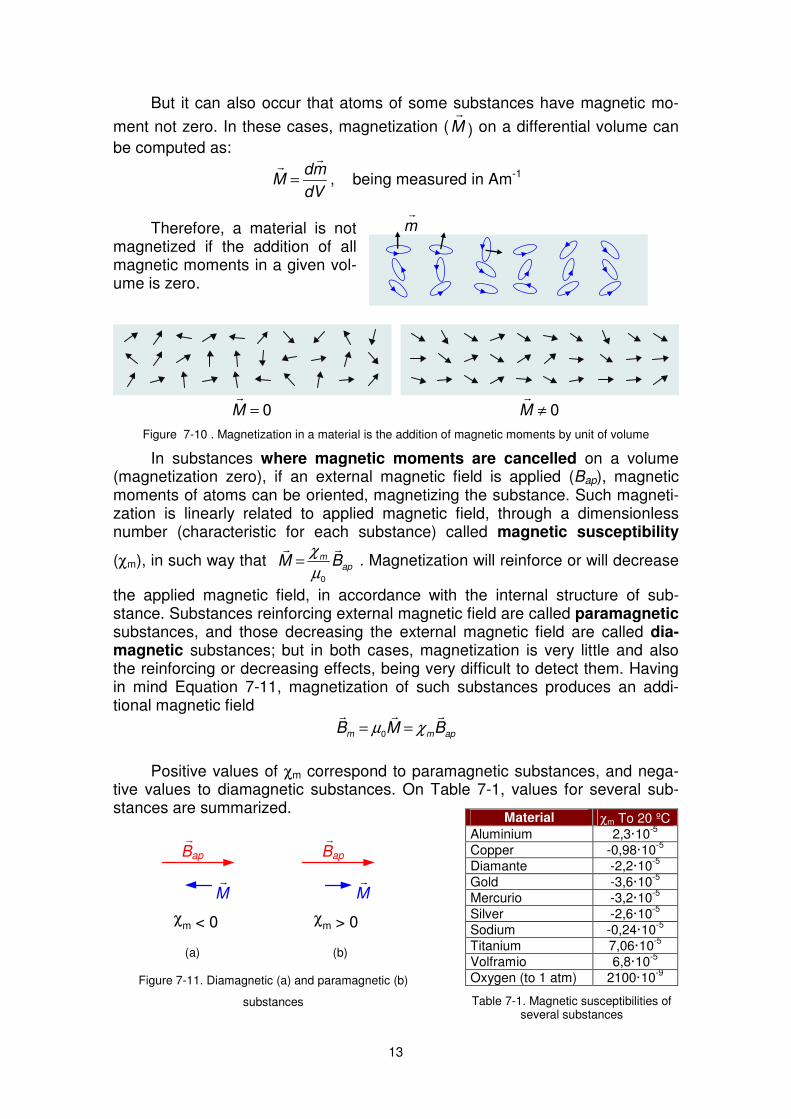
In substances where magnetic moments are cancelled on a volume (magnetization zero), if an external magnetic field is applied (Bap), magnetic moments of atoms can be oriented, magnetizing the substance. Such magneti-zation is linearly related to applied magnetic field, through a dimensionless number (characteristic for each substance) called magnetic susceptibility

(χm), in such way that apm BM

rr

0µ

χ= . Magnetization will reinforce or will decrease

the applied magnetic field, in accordance with the internal structure of sub-stance. Substances reinforcing external magnetic field are called paramagnetic substances, and those decreasing the external magnetic field are called dia-magnetic substances; but in both cases, magnetization is very little and also the reinforcing or decreasing effects, being very difficult to detect them. Having in mind Equation 7-11, magnetization of such substances produces an addi-tional magnetic field

apmm BMBrrr

χµ == 0

Positive values of χm correspond to paramagnetic substances, and nega-tive values to diamagnetic substances. On Table 7-1, values for several sub-stances are summarized.

Material χm To 20 ºC Aluminium 2,3·10

-5

Copper -0,98·10-5

Diamante -2,2·10-5

Gold -3,6·10-5

Mercurio -3,2·10-5

Silver -2,6·10-5

Sodium -0,24·10-5

Titanium 7,06·10-5

Volframio 6,8·10-5

Oxygen (to 1 atm) 2100·10-9

Table 7-1. Magnetic susceptibilities of several substances

r

Bap

r

M

χm < 0

r

Bap

r

M

χm > 0

(b)(a)

Figure 7-11. Diamagnetic (a) and paramagnetic (b)

substances

r

m

14

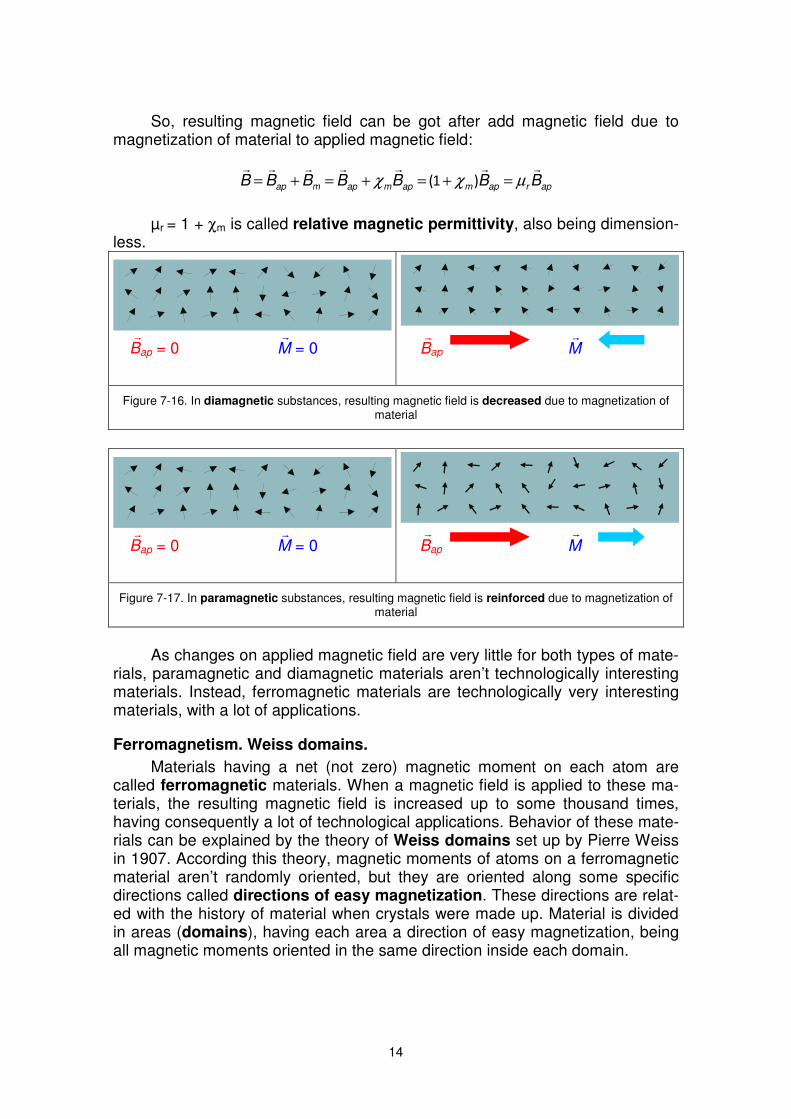
So, resulting magnetic field can be got after add magnetic field due to

magnetization of material to applied magnetic field:

aprapmapmapmap BBBBBBBrrrrrrr

µχχ =+=+=+= )1(

µr = 1 + χm is called relative magnetic permittivity, also being dimension-less.

rBap = 0

rM = 0

rBap

rM

Figure 7-16. In diamagnetic substances, resulting magnetic field is decreased due to magnetization of material

rBap = 0

rM = 0

r

Bap r

M

Figure 7-17. In paramagnetic substances, resulting magnetic field is reinforced due to magnetization of material

As changes on applied magnetic field are very little for both types of mate-rials, paramagnetic and diamagnetic materials aren’t technologically interesting materials. Instead, ferromagnetic materials are technologically very interesting materials, with a lot of applications.

Ferromagnetism. Weiss domains.

Materials having a net (not zero) magnetic moment on each atom are called ferromagnetic materials. When a magnetic field is applied to these ma-terials, the resulting magnetic field is increased up to some thousand times, having consequently a lot of technological applications. Behavior of these mate-rials can be explained by the theory of Weiss domains set up by Pierre Weiss in 1907. According this theory, magnetic moments of atoms on a ferromagnetic material aren’t randomly oriented, but they are oriented along some specific directions called directions of easy magnetization. These directions are relat-ed with the history of material when crystals were made up. Material is divided in areas (domains), having each area a direction of easy magnetization, being all magnetic moments oriented in the same direction inside each domain.

15

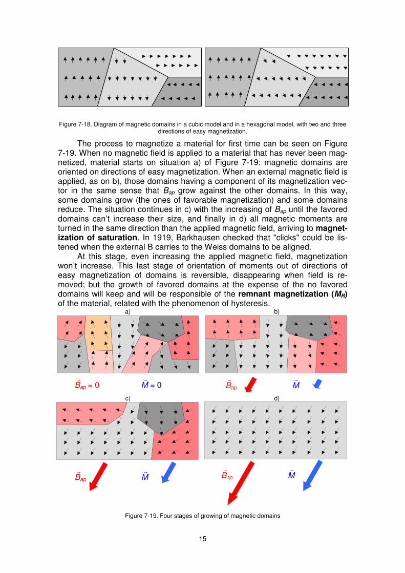
Figure 7-18. Diagram of magnetic domains in a cubic model and in a hexagonal model, with two and three directions of easy magnetization.

The process to magnetize a material for first time can be seen on Figure 7-19. When no magnetic field is applied to a material that has never been mag-netized, material starts on situation a) of Figure 7-19: magnetic domains are oriented on directions of easy magnetization. When an external magnetic field is applied, as on b), those domains having a component of its magnetization vec-tor in the same sense that Bap grow against the other domains. In this way, some domains grow (the ones of favorable magnetization) and some domains reduce. The situation continues in c) with the increasing of Bap until the favored domains can’t increase their size, and finally in d) all magnetic moments are turned in the same direction than the applied magnetic field, arriving to magnet-ization of saturation. In 1919, Barkhausen checked that "clicks" could be lis-tened when the external B carries to the Weiss domains to be aligned.

At this stage, even increasing the applied magnetic field, magnetization won’t increase. This last stage of orientation of moments out of directions of easy magnetization of domains is reversible, disappearing when field is re-moved; but the growth of favored domains at the expense of the no favored domains will keep and will be responsible of the remnant magnetization (MR) of the material, related with the phenomenon of hysteresis.

a)

r

Bap = 0 r

M = 0

b)

rBap

rM

c)

rBap

rM

d)

rBap

rM

Figure 7-19. Four stages of growing of magnetic domains

16

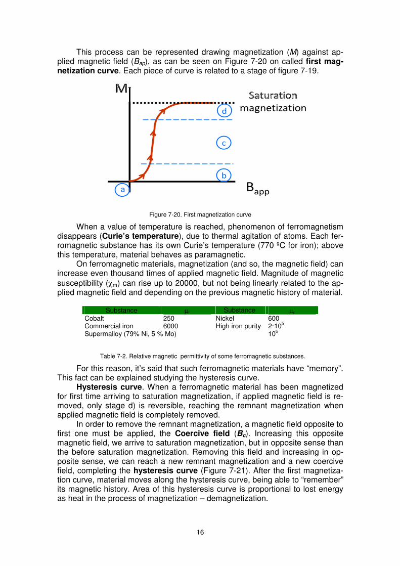
This process can be represented drawing magnetization (M) against ap-plied magnetic field (Bap), as can be seen on Figure 7-20 on called first mag-netization curve. Each piece of curve is related to a stage of figure 7-19.

Figure 7-20. First magnetization curve

When a value of temperature is reached, phenomenon of ferromagnetism disappears (Curie’s temperature), due to thermal agitation of atoms. Each fer-romagnetic substance has its own Curie’s temperature (770 ºC for iron); above this temperature, material behaves as paramagnetic.

On ferromagnetic materials, magnetization (and so, the magnetic field) can increase even thousand times of applied magnetic field. Magnitude of magnetic

susceptibility (χm) can rise up to 20000, but not being linearly related to the ap-plied magnetic field and depending on the previous magnetic history of material.

Substance µr Substance µr Cobalt 250 Nickel 600 Commercial iron 6000 High iron purity 2·10

5

Supermalloy (79% Ni, 5 % Mo) 106

Table 7-2. Relative magnetic permittivity of some ferromagnetic substances.

For this reason, it’s said that such ferromagnetic materials have “memory”. This fact can be explained studying the hysteresis curve.

Hysteresis curve. When a ferromagnetic material has been magnetized for first time arriving to saturation magnetization, if applied magnetic field is re-moved, only stage d) is reversible, reaching the remnant magnetization when applied magnetic field is completely removed.

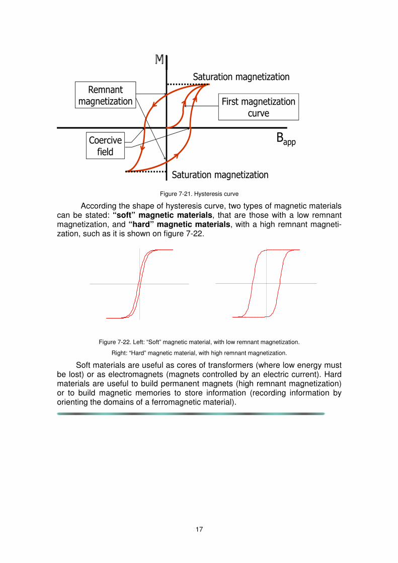
In order to remove the remnant magnetization, a magnetic field opposite to first one must be applied, the Coercive field (Bc). Increasing this opposite magnetic field, we arrive to saturation magnetization, but in opposite sense than the before saturation magnetization. Removing this field and increasing in op-posite sense, we can reach a new remnant magnetization and a new coercive field, completing the hysteresis curve (Figure 7-21). After the first magnetiza-tion curve, material moves along the hysteresis curve, being able to “remember” its magnetic history. Area of this hysteresis curve is proportional to lost energy as heat in the process of magnetization – demagnetization.

17

Figure 7-21. Hysteresis curve

According the shape of hysteresis curve, two types of magnetic materials can be stated: “soft” magnetic materials, that are those with a low remnant magnetization, and “hard” magnetic materials, with a high remnant magneti-zation, such as it is shown on figure 7-22.

Figure 7-22. Left: “Soft” magnetic material, with low remnant magnetization.

Right: “Hard” magnetic material, with high remnant magnetization.

Soft materials are useful as cores of transformers (where low energy must be lost) or as electromagnets (magnets controlled by an electric current). Hard materials are useful to build permanent magnets (high remnant magnetization) or to build magnetic memories to store information (recording information by orienting the domains of a ferromagnetic material).

18

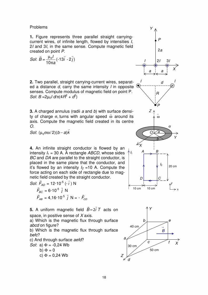
Problems 1. Figure represents three parallel straight carrying-current wires, of infinite length, flowed by intensities I, 2I and 3I, in the same sense. Compute magnetic field created on point P.

Sol: )2(-1310

0 j-ia

I=B

rrr

π

µ

2. Two parallel, straight carrying-current wires, separat-ed a distance d, carry the same intensity I in opposite senses. Compute modulus of magnetic field on point P.

Sol: B =2µ0I d/π(4R2 + d2) 3. A charged annulus (radii a and b) with surface densi-

ty of charge σ, turns with angular speed ωr

around its axis. Compute the magnetic field created in its centre O.

Sol: kabr

))(2/( 0 −σωµ

4. An infinite straight conductor is flowed by an intensity I1 = 30 A. A rectangle ABCD, whose sides BC and DA are parallel to the straight conductor, is placed in the same plane that the conductor, and it’s flowed by an intensity I2 =10 A. Compute the force acting on each side of rectangle due to mag-netic field created by the straight conductor.

Sol: ADFr

= 12·10-5 (- ir

) N

BCFr

= 6·10-5 jr

N

ABFr

= 4,16·10-5 jr

N = - CDFr

5. A uniform magnetic field TiBrr

2= acts on

space, in positive sense of X axis. a) Which is the magnetic flux through surface abcd on figure? b) Which is the magnetic flux through surface befc? c) And through surface aefd?

Sol: a) Φ = -0,24 Wb

b) Φ = 0

c) Φ = 0,24 Wb

a a

I 2I 3I

P

2a

Y

X

R

P

d II

X

Y

Z

O a

b

σ

r

ω

I1

10 cm 10 cm

20 cmI2

A B

D C

x

y

r

B

X

Y

Z

30 cm

40 cm

50 cm

a

b e

fc

d

19

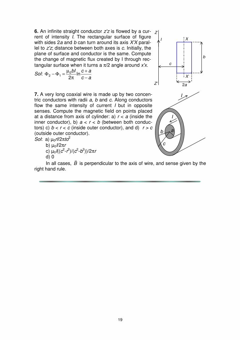
6. An infinite straight conductor z'z is flowed by a cur-rent of intensity I. The rectangular surface of figure with sides 2a and b can turn around its axis X'X paral-lel to z'z; distance between both axes is c. Initially, the plane of surface and conductor is the same. Compute the change of magnetic flux created by I through rec-

tangular surface when it turns a π/2 angle around x'x.

Sol: ac

acbI

−

+

π

µ=Φ−Φ ln

20

12

7. A very long coaxial wire is made up by two concen-tric conductors with radii a, b and c. Along conductors flow the same intensity of current I but in opposite senses. Compute the magnetic field on points placed at a distance from axis of cylinder: a) r < a (inside the inner conductor), b) a < r < b (between both conduc-tors) c) b < r < c (inside outer conductor), and d) r > c (outside outer conductor).

Sol: a) µ0rI/2πto2

b) µ0I/2πr

c) µ0I((c2-r2)/(c2-b2))/2πr

d) 0

In all cases, Br

is perpendicular to the axis of wire, and sense given by the right hand rule.

I

Z

Z’

X

X’

c

b

2a

I

I

ab

c

20

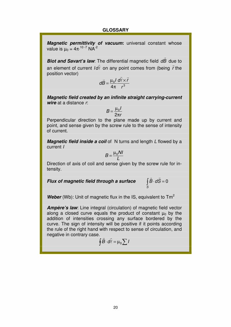
GLOSSARY

Magnetic permittivity of vacuum: universal constant whose

value is µ0 = 4π⋅10 -7 NA-2

Biot and Savart’s law: The differential magnetic field Bdr

due to

an element of current I l

r

d on any point comes from (being rr

the position vector)

30

4 r

rdIBd

rlr

r ×

π

µ=

Magnetic field created by an infinite straight carrying-current wire at a distance r:

r

IB

π

µ=

20

Perpendicular direction to the plane made up by current and point, and sense given by the screw rule to the sense of intensity of current. Magnetic field inside a coil of N turns and length L flowed by a current I

L

NIB 0µ

=

Direction of axis of coil and sense given by the screw rule for in-tensity.

Flux of magnetic field through a surface 0=⋅∫S

SdBrr

Weber (Wb): Unit of magnetic flux in the IS, equivalent to Tm2 Ampère’s law: Line integral (circulation) of magnetic field vector along a closed curve equals the product of constant µ0 by the addition of intensities crossing any surface bordered by the curve. The sign of intensity will be positive if it points according the rule of the right hand with respect to sense of circulation, and negative in contrary case.

∫ ∑µ=⋅ IdB 0l

rr